the Creative Commons Attribution 4.0 License.
the Creative Commons Attribution 4.0 License.
 | 05 Dec 2022
Equatorial waves resolved by balloon-borne Global Navigation Satellite System radio occultation in the Strateole-2 campaign
Jennifer S. Haase
Michael J. Murphy
M. Joan Alexander
Martina Bramberger
Albert Hertzog
Current climate models have difficulty representing realistic wave–mean flow interactions, partly because the contribution from waves with fine vertical scales is poorly known. There are few direct observations of these waves, and most models have difficulty resolving them. This observational challenge cannot be addressed by satellite or sparse ground-based methods. The Strateole-2 long-duration stratospheric superpressure balloons that float with the horizontal wind on constant-density surfaces provide a unique platform for wave observations across a broad range of spatial and temporal scales. For the first time, balloon-borne Global Navigation Satellite System (GNSS) radio occultation (RO) is used to provide high-vertical-resolution equatorial wave observations. By tracking navigation signal refractive delays from GPS satellites near the horizon, 40–50 temperature profiles were retrieved daily, from balloon flight altitude (∼20 km) down to 6–8 km altitude, forming an orthogonal pattern of observations over a broad area (±400–500 km) surrounding the flight track. The refractivity profiles show an excellent agreement of better than 0.2 % with co-located radiosonde, spaceborne COSMIC-2 RO, and reanalysis products. The 200–500 m vertical resolution and the spatial and temporal continuity of sampling make it possible to extract properties of Kelvin waves and gravity waves with vertical wavelengths as short as 2–3 km. The results illustrate the difference in the Kelvin wave period (20 vs. 16 d) in the Lagrangian versus ground-fixed reference and as much as a 20 % difference in amplitude compared to COSMIC-2, both of which impact estimates of momentum flux. A small dataset from the extra Galileo, GLONASS, and BeiDou constellations demonstrates the feasibility of nearly doubling the sampling density in planned follow-on campaigns when data with full equatorial coverage will contribute to a better estimate of wave forcing on the quasi-biennial oscillation (QBO) and improved QBO representation in models.
- Article
(8921 KB) - Full-text XML
- BibTeX
- EndNote


The fine vertical scales of atmospheric waves in the upper troposphere–lower stratosphere (UTLS) region create observational challenges that cannot be addressed by either satellite or sparse ground-based observations (Vincent and Alexander, 2020). Modeling challenges persist due to the high resolution required to simulate waves and gaps in physical-process understanding (Bushell et al., 2020). This work introduces the deployment of the next-generation Global Navigation Satellite System (GNSS) Radio OCcultation (ROC) instrument on board long-duration stratospheric balloons to sample the equatorial wave field in three dimensions by retrieving a continuous sequence of temperature profiles on both sides of the balloon trajectory. The balloon-borne ROC observations from the Strateole-2 project enable investigations to quantify UTLS wave properties that are needed to improve model representations of wave driving of the quasi-biennial oscillation (QBO). They also enable investigations to determine the relationship of UTLS waves to thin cirrus clouds that can be used for improving the representation of waves in models. This can be advanced by quantifying the global characteristics of waves that determine tropical cold-point temperature variability for use in improving models of stratospheric dehydration (Kim and Alexander, 2015; Jensen et al., 2017).
Tropical waves in the UTLS have climate and weather impacts through their effects on cirrus clouds, stratospheric dehydration, and wave-driven circulation patterns. In particular, the QBO is a wave-driven circulation pattern with clear oscillations in the zonal-mean equatorial zonal wind with a typical period of 27 months (Baldwin et al., 2001). It is the dominant mode of interannual lower stratospheric wind variability, affecting tropospheric variability through various teleconnections. The deposition of momentum by the dissipation of tropical waves of a variety of scales is believed to be the main cause. However, current climate models with limited resolution have difficulties producing a realistic QBO in the lower stratosphere due to unresolved small-scale waves (Antonita et al., 2008; Ern and Preusse, 2009; Alexander and Ortland, 2010; Ern et al., 2014; Richter et al., 2020), leading to uncertainty in the evolution of the QBO period and amplitude in a changing climate. Direct observations that can inform the process of wave driving of the QBO are rare. The lowermost QBO winds have shown evidence of weakening in recent decades (Kawatani and Hamilton, 2013), and models suggest the cause may be a gradual strengthening of the wave-driven stratospheric overturning circulation. However, this overturning cannot be directly observed, and the wave mean–flow interactions that drive the stratospheric circulation are plagued by uncertainties associated with a lack of knowledge of the wave properties.
Limb-sounding satellite observations have led to key advances in understanding equatorial waves, in part due to their high vertical resolution capable of resolving detailed vertical variations (Salby et al., 1984; Shiotani et al., 1997; Srikanth and Ortland, 1998; Ern et al., 2008; Alexander et al., 2010). GNSS radio occultation (RO) is one of these limb-sounding techniques that has had a particularly extensive impact because of the large and steadily increasing number of satellites now providing temperature and refractivity profiles to study atmospheric waves in the stratosphere (e.g., Tsuda et al., 2000; Randel et al., 2003, 2021). The RO technique is based on the principle that the refractive bending and propagation delay of a transmitted navigation signal to a receiver on a low-Earth-orbit (LEO) satellite is measured each time the LEO sets or rises relative to GNSS satellites. The bending angle is inverted to produce an estimate of refractivity in a layered approximation of the Earth atmosphere, from which the atmospheric pressure and temperature can be derived (Kursinski et al., 1997; Fjeldbo and Eshleman, 1968). Theoretically, the vertical resolution of the RO method depends on the gradient of the bending angle with height and thus the gradient of refractivity with height, and it is estimated to be as fine as 100–200 m based on the diameter of the first Fresnel zone at L-band frequencies (Kursinski et al., 1997). However, the measurements at individual tangent point heights are not independent because the ray path samples all atmospheric layers above the tangent point, so the actual resolution is lower. Previous studies have estimated that the typical vertical resolution of spaceborne RO varies from 100 m near the surface to 1 km at the tropopause (Zeng et al., 2012).
Multiple spaceborne missions have deployed GPS receivers on LEO satellites to perform RO observations. The combination of these missions provides a large number of profiles of neutral atmospheric refractivity, temperature, moisture, and ionospheric electron density. Moreover, multiple GNSS constellations are now operational, including GPS, GLONASS, Galileo, and BeiDou, which provide more opportunities for RO observations. The Tri-GNSS (TriG) receiver on COSMIC-2 (Schreiner et al., 2020) can now provide profiles from GLONASS as well as GPS, and Galileo profiles have been demonstrated from aircraft (Haase et al., 2021). The global coverage and high vertical resolution of the spaceborne RO datasets have provided the opportunity to quantify the global properties of gravity waves and wave sources of variability in the stratosphere. Reviews of the success of RO in capturing equatorial waves are provided in Ho et al. (2019) and Scherllin-Pirscher et al. (2021) and references therein. Several of these studies retrieved information on individual wave events but were limited to waves with very large horizontal scales and typically greater than 4 km vertical wavelength because the spacing between profiles is irregular and quasi-random in time and space. There is a continuing need to increase the vertical resolution to gain a complete view of the fine-scale wave–mean flow interaction that is unresolved in global models. For example, in QBO shear zones, wave vertical wavelengths will shrink wherever the wind approaches the wave phase speed. If the wave can survive to higher altitudes where density is lower and the wave has shorter vertical wavelengths, the wave can impart a significantly stronger force on the QBO flow (Vincent and Alexander, 2020).
The need for coherent sampling of wave structures in time and space with higher vertical resolution motivates the implementation of balloon-borne RO observations. The technique has the added advantage of sampling the atmosphere in three dimensions, i.e., to both sides of the flight path along the line of sight to setting and rising GNSS satellites (Haase et al., 2021). Because the balloon carrying the receiver moves at significantly slower speeds than the GNSS satellite, the location of the tangent point (point on a signal ray path closest to the Earth) drifts horizontally from the balloon position at flight level to as much as 500 km from the flight path as the tangent point descends to a height of 4 km. The resulting slanted profile measurements provide an advantage in 3D sampling at the expense of added complexity in interpreting the profiles because of the potential distortion of retrieved wave parameters, such as wavelength and momentum flux (de la Torre et al., 2018). The slanted nature of the profiles also presents difficulties in resolving wave properties in the presence of horizontal-scale variability shorter than ∼1000 km, without explicitly considering the drift. The distortion is minimal for larger-scale tropical waves, which are the subject of this study.
This study is organized as follows: Sect. 2 briefly describes the methodology of balloon-borne RO. Section 3 gives an overview of the superpressure balloon flights in the Strateole-2 campaign and the balloon-borne ROC instrument. Section 4 introduces the data analysis procedures and estimates the vertical resolution of balloon-borne RO. Section 5 presents comparisons of the profiles with other independent datasets from radiosondes and spaceborne RO, as well as comparisons with numerical model reanalyses. Section 6 presents the results illustrating the equatorial waves that are captured with different periods and scales. Section 7 discusses some future perspectives and limitations of the balloon-borne RO observations. Conclusions summarizing the results are presented in Sect. 8.
The GNSS RO technique is a powerful remote sensing technique that utilizes GNSS signals that are refracted and delayed as they traverse the atmosphere nearly horizontally. Vertical variations in atmospheric refractivity and other properties are derived from the signal propagation delays. As a GNSS satellite sets (or rises) relative to a receiver on an airborne or spaceborne platform, the navigation signal scans through the highest to lowest atmospheric layers (or vice versa), which yields a complete profile. In the following, we refer to airborne RO and balloon-borne RO as ARO and BRO, respectively, when necessary to distinguish them from spaceborne RO, which we will refer to as SRO. Unlike SRO, slower platforms flying inside the atmosphere, such as aircraft (Haase et al., 2014, 2021) and balloons (Haase et al., 2012) provide a unique opportunity to perform RO measurements continuously in time and space over a localized area, rather than the pseudo-random distribution of the global SRO datasets. The density and continuity are advantageous for reconnaissance flights in an area of interest, such as at the locations of hurricanes (Murphy et al., 2015; Chen et al., 2018) and atmospheric rivers (Ralph et al., 2020), but can also be applied to the problem of resolving fine-scale wave structures from free-floating balloons. The physics and geometry of ARO and BRO are similar to those of SRO, but there are some geometric modifications required to implement the typical RO retrieval technique. Detailed descriptions of the geometry and theory of BRO are provided in Appendix A.
The atmospheric refractivity N for radio waves at GNSS frequencies (L band) in the neutral atmosphere is described by (Rüeger, 2002)
where n is the refractive index and p, pw, and T are atmospheric pressure (in hPa), water vapor pressure (in hPa), and temperature (in K), respectively. In the atmosphere higher than ∼10 km, assuming water vapor is negligible, the equation for refractivity can be simplified to
where Td is commonly referred to as dry temperature and deviates from the true temperature if moisture is present.
The atmosphere is generally in hydrostatic equilibrium, where the pressure gradient force balances with gravity if there is no acceleration in the vertical direction. It is described by the following equation:
where ρ is the atmospheric density. When the atmosphere is perturbed by waves, this equilibrium is no longer satisfied. This is true for high-frequency gravity waves with shorter horizontal wavelengths, and the vertical accelerations cannot be neglected in the vertical motion of perturbation. However, lower-frequency gravity waves with longer horizontal wavelengths, such as inertia gravity waves, have small vertical accelerations and are consistent with the quasi-hydrostatic approximation.
In this study, dry temperature and pressure were retrieved based on the simplified refractivity formula (Eq. 2), hydrostatic equilibrium (Eq. 3), and the ideal gas law p=ρRT, and R is the ideal gas constant. The dry temperature is derived from the following integral:
where g(z) is gravitational acceleration as a function of height and is the ratio of refractivity of two different altitudes. N(h0) and T(h0) are refractivity and temperature, respectively, at the balloon flight altitude h0 calculated from in situ measurements.
Strateole-2 (STR-2) is an international multi-year series of campaigns that utilize long-duration stratospheric superpressure balloons (SPBs) to investigate the atmospheric dynamics and composition of the tropical tropopause layer (TTL) (Haase et al., 2018). The SPBs fly for several months along the equatorial belt at altitudes of 18–20 km. They are advected by the wind on constant-density surfaces and therefore behave as quasi-Lagrangian tracers in the atmosphere. The first preparatory campaign began in November 2019 with the practical objective of testing the unique capabilities of each of the instrument configurations in advance of the full scientific deployments. Five different instrument configurations were tested on the balloons; some provided in situ information on the physics, dynamics, particle counts, and greenhouse gas composition of the sampled air parcels surrounding the balloons. Other instruments, including the ROC instrument described here, also sampled the atmosphere below the balloons. The preparatory campaign provided initial observations to assess the capabilities of the flotilla to reveal the nature of equatorial waves.
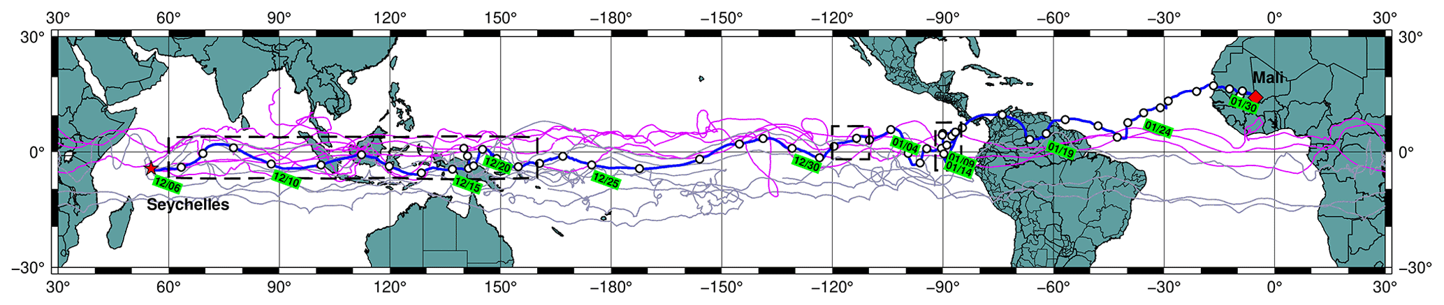
Figure 1Trajectories of all balloons launched in the Strateole-2 2019 campaign. The thick blue line is balloon ST2_C0_06_STR1 that carried the radio occultation receiver. The red star marks the launch site in Seychelles, and the red diamond indicates the final landing site in Mali. Small circles over the trajectory indicate 00Z each day and are labeled at 5 d intervals. Dashed boxes along the trajectory mark the periods when BRO data were recovered. Gray lines are the four other balloons flying at ∼20 km, and magenta lines are the three balloons flying at ∼18 km.
3.1 Superpressure balloon flights
Eight SPBs were launched from Mahé, Seychelles (4.7∘ S, 55.5∘ E), in the western Indian Ocean over the period from November to December 2019, and they flew until late February 2020, achieving a mean flight duration in the tropics of nearly 3 months (85 d). The flight tracks of these balloons are shown in Fig. 1. Several balloons completed more than one full circumnavigation at the Equator. The 13 m diameter balloon (labeled “ST2_C0_06_STR1”) that carried the BRO instrument was launched on 5 December 2019 and flew eastward at about 20 km altitude for 57 d. Due to a small helium leak in the balloon, it was terminated for safety reasons over the desert in Mali, Africa, on 2 February 2020. The data were transmitted during flight, and the instrumentation was not recovered.
The balloon carrying ROC equipment also carried the Balloonborne Cirrus and convective overshOOt Lidar (BeCOOL) system to measure optical properties of cirrus in the nadir-viewing mode and the topography of convective cloud tops (Ravetta et al., 2020), as well as the BOLometer Determining Albedo and InfraRed flux (BOLDAIR) to measure upward longwave and shortwave radiative fluxes. The combination of instruments was selected to better understand the modulation of cirrus by wave motions and assess the radiative heating and forcing of the lower stratosphere by water vapor anomalies. The Thermodynamical SENsor (TSEN) meteorological package was included on all balloons to provide in situ measurements which can be used to derive the intrinsic frequency spectrum and probability distribution of gravity wave momentum flux at flight level (Podglajen et al., 2016; Hertzog et al., 2008; Corcos et al., 2021). The ROC observations would augment these studies by providing continuous temperature profiles underneath the flight track to resolve the vertical variations. The same instruments flew in late 2021 and will be flown in the forthcoming campaign in late 2024 with 20 balloons to capture different phases of the QBO.
3.2 Instrumentation
The ROC (Radio OCcultation) version 2 receiver builds on the heritage of the GPS-only ROC receiver that was originally deployed in the Concordiasi campaign in Antarctica (Haase et al., 2012; Rabier et al., 2010). It is a low-cost, lightweight multi-GNSS receiver capable of tracking multiple constellations and frequencies with two antennas. It utilizes the sophisticated Septentrio AsteRx4 OEM board, which performs phase-locked loop (PLL) tracking of all GNSS signals in the field of view and is configured to record down to a elevation angle below the horizon from the balloon at ∼20 km altitude. It also contains a Linux single-board computer (TS-7680) to manage onboard power, configuration, data acquisition, storage, and communication. The superpressure balloons are composed of two gondolas, “Zephyr” for the science payload and “Euros” for flight control. The ROC receiver enclosure was installed inside the Zephyr gondola and connected to the two avionic GNSS antennas manufactured by GPS Source, which were installed on the top of the gondola tilted 30∘ from the horizontal in opposite directions. The GNSS antennas were separated as far as possible from the Iridium antenna on the ∼50 cm wide gondola to avoid electromagnetic interference because of the proximity of their frequency bands. Also installed in the Zephyr gondola were two other scientific instruments, BOLDAIR and BeCOOL, and the Zephyr on-board computer (OBC), which managed the solar-powered battery charging system and the data and command telemetry through the Iridium satellite link. The data were recovered at the Zephyr Mission Control Centre (CCMz) managed by the Laboratoire de Météorologie Dynamique (LMD) of the Centre Nationale de la Recherche Scientifique (CNRS) in France. The TSEN package included an U-blox single-frequency GPS receiver on the gondola to provide timing and wind velocity through real-time positioning solutions. The TSEN thermistor and thermocouple were suspended 8 m below the Zephyr gondola to provide in situ measurements of ambient temperature at 30 s sampling intervals, and the TSEN barometer was located above the Euros gondola, measuring pressure at the same data rate.
3.3 Dataset
The ROC receiver continuously tracked multiple constellations including GPS, Galileo, and GLONASS and logged the carrier phase, pseudorange, and signal-to-noise ratio (SNR) at a 5 s sampling interval throughout the whole flight. The logged data were stored in the internal storage of the ROC receiver and were transmitted by an Iridium data link to the CCMz every hour. Due to a technical problem that limited the bandwidth of the Iridium satellite link, data from only 23 d of the 57 d flight were recovered. The recovered dataset includes GPS-only data from 6–22 December 2019 (largest box on the left in Fig. 1), 1 January 2020 (box in the middle in Fig. 1), and 9 and 11–14 January 2021 (box on the right in Fig. 1). The data from three constellations (GPS, GLONASS, Galileo) were recovered on 15 December 2019. A 12 h test was implemented on 14 January 2021 and recovered data from the GPS and BeiDou constellations.
4.1 Retrieval procedures
The precise 3D positions of the balloon were calculated from the GPS pseudorange and carrier-phase data using precise point positioning with ambiguity resolution (PPPAR) (Ge et al., 2008; Geng et al., 2019) using the Position And Navigation Data Analyst (PANDA) software package developed at Wuhan University (Shi et al., 2008). The procedure was carried out in three steps. The first step was to estimate high-rate (30 s) satellite clock errors based on regional data, instead of using global satellite clock products, since the estimated regional clock solutions can compensate for other unmodeled errors in the PPPAR solution (Lou et al., 2014). GPS satellite orbits were fixed to the Center for Orbit Determination in Europe (CODE) final orbits (Dach et al., 2020). Ground GPS observations were used from a list of 26 stations from the International GNSS Service (IGS) network in the equatorial region around the balloon trajectory to solve for the clock parameters (see Fig. D1 in Appendix D).
In the next step, fractional cycle biases (FCBs) were estimated from the same dataset to improve the resolution of the carrier-phase ambiguities (Geng et al., 2011). The final calculation was solved for the coordinates of the balloon antenna at each time sample. The receiver clock errors were also estimated at each epoch as parameters with white noise variance. The zenith hydrostatic delay is constrained to the Saastamoinen model (Saastamoinen, 1972), and the zenith wet delay is assumed to be negligible at the balloon flight altitude and thus not included in the procedures, which reduces the number of estimated parameters. The estimated position accuracy is ∼10 cm in the horizontal, ∼20 cm in the vertical, and 0.05 m s−1 in velocity. The precise position calculation was shown to be a significant improvement over the onboard real-time GPS solution. It has been used to improve the calculation of gravity wave momentum flux from balloon motion variations that treat the balloon as a quasi-Lagrangian tracer (Zhang et al., 2016).
After the precise 3D positions were determined, they were fixed in the positioning software to calculate the residual distance (excess phase) between the geometric balloon-to-satellite distance and the observed carrier phase using the same satellite clock corrections and models for relativity, antenna phase center corrections, and other effects that were used in the position calculation. The ionospheric effects were corrected using the ionosphere-free combination of dual-frequency (L1 and L2) observations. The excess Doppler for each satellite was calculated by differentiating the excess phase with respect to time. The receiver clock errors were removed by single differencing, where the excess Doppler time series from a high-elevation satellite in view at the same time was subtracted from the occulting-satellite time series. A second-order Savitzky–Golay filter was used to smooth high-frequency noise in the excess Doppler that would lead to unrealistic variability in the scale shorter than the first Fresnel zone. The filtering window width was selected to be 55 s based on the vertical resolution analysis in the later sections.
The local radius of curvature, Rc, tangent to the ellipsoidal Earth surface was determined at the approximate location of the lowest tangent point with an orientation parallel to the occultation plane (Syndergaard, 1998). The Cartesian coordinates of the satellite and balloon at each epoch were offset to the new reference frame with the origin at the center of curvature. The refractivity at the balloon flight level, N(h0), was calculated from the in situ pressure and temperature based on Eq. (2) and averaged over the occultation duration to reduce sensitivity to small variations in flight altitude over the duration of the occultation.
The excess Doppler shift was projected onto the satellite-receiver velocities in the shifted coordinate system to calculate the bending angle as a function of impact parameter a=n(r)r as described in Appendix A. Balloon positions and velocities were smoothed using the same filter as the excess Doppler. The refractive index at the balloon location was . The bending angle was then interpolated to an even sampling of 10 m in the impact parameter. The bending angle was calculated from the satellite observations from 10∘ above the local horizontal until the signal was lost, so it included both positive and negative elevation angles (see Fig. A1). The partial bending angle, α′, at each impact parameter, a, below the flight level of the balloon was calculated by subtracting the positive elevation angle observations from the negative elevation angle observations for the same impact parameter (Healy et al., 2002). Finally, a was converted to height above the ellipsoid using a=n(r)r and . The ellipsoidal height was then converted to the mean sea level (MSL) height by subtracting the geoid height () retrieved from the EGM96 geoid model at the location of the lowest tangent point. The EGM96 model has a stated accuracy of ∼10 cm and horizontal resolution of 15′ (Lemoine et al., 1998).
In practice, even after filtering, the noise in the balloon velocity estimate creates noise in the excess Doppler for positive elevation angles that is comparable to the magnitude of the accumulated excess Doppler due to the atmosphere, so the derived bending angle can be very noisy. In order to reduce this noise, the bending angle as a function of time was heavily smoothed with a LOESS filter (locally weighted quadratic regression fit) over a 5 min moving window from to telmax, corresponding to the time when the tangent point was 1 km below flight level to the time of maximum positive elevation angle. The bending angle was lightly smoothed with a 1.25 min window for the remaining period for the negative elevation angle. A taper function was used to merge the two bending angle time series between and . Then we calculated the partial bending angle, which was then much less noisy for all tangent point heights, and computed the refractive index using the inverse Abel transform (Eq. A3), with the refractive index nR at the balloon height fixed. This final estimate of the refractive index should be considered strongly constrained by the in situ refractive index for the top 0.5 to 1 km (Murphy, 2015). These improvements to the bending angle, partial bending angle, and refractivity calculations produce less bias compared to the previous versions of the ARO inversion software developed by Xie et al. (2008) and Murphy et al. (2015), which has been used in multiple aircraft campaigns (Haase et al., 2014, 2021).
The 1D-Var algorithm based on the Bayesian optimal estimation theory by combining RO observations and a priori information from a model can be implemented to retrieve a complete set of meteorological parameters, including water vapor pressure (Poli et al., 2002). However, we chose to use dry temperature to avoid any dependence of the retrieval on a first-guess model that did not contain any wave signature, since the region of interest is above 10 km and BRO is not accurate enough to be sensitive to low values of water vapor at those altitudes. This also makes it possible to compare BRO dry-temperature profiles directly to SRO dry-temperature profiles. The dry-temperature profiles were calculated from refractivity and in situ pressure and temperature using Eq. (4).
Because the motion of the GNSS satellite is much greater than that of the balloon during an occultation, the tangent points drift horizontally away from the balloon as the ray paths from a setting satellite descend through the atmosphere or towards the balloon for a rising satellite, as shown in Fig. B1. For SRO, where the receiver is in a vacuum and the occultation geometry is symmetric within the atmosphere, the horizontal location of the tangent points of each ray path can be solved geometrically. However, this is not the case for BRO, where the receiver is within the atmosphere. The horizontal location at a given tangent point height is determined by a simulation using forward ray tracing implemented in the Radio Occultation Simulator for Atmospheric Profiling (ROSAP) model (Hoeg et al., 1996; Syndergaard, 1998), assuming a climatological refractivity profile from the CIRA+Q model appropriate for the month and latitude (Kirchengast et al., 1999). The final BRO slant profile dataset includes a horizontal location (latitude and longitude) and time for each tangent point height in the profile, and the location and time of the lowest tangent point of the profile are provided as the reference for the profile.
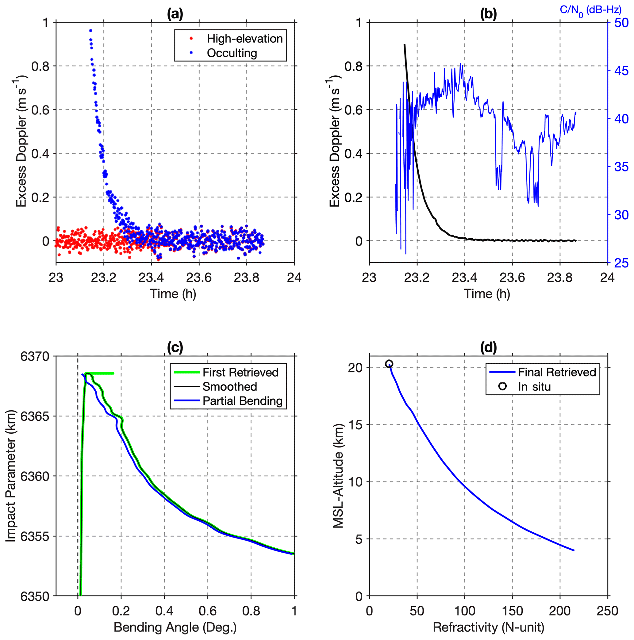
Figure 2(a) Excess Doppler for the pair of satellites from the rising occultation G29r_G13. The GPS satellite PRN29 is in the occultation position, and satellite PRN13 at a high elevation angle is used to remove the receiver clock error. (b) The excess Doppler difference for G29 minus G13, after interpolation and filtering (left axis), and signal carrier-to-noise ratio () (right axis). (c) The bending angle from the initial retrieval (light green) and final retrieval (black) with tapered increased smoothing for the top and positive elevation angle segments of the bending angle (see text). The partial bending angle (blue) is derived from the black curve. (d) The final retrieved refractivity profile with refractivity at the top fixed to the balloon in situ measurement.
Figure 2 shows the intermediate products of excess Doppler and bending angle for a rising occultation labeled “G29r_G13”. This occultation lasted about 15 min from when the receiver started tracking satellite PRN29 until it rose above the local horizontal. The undifferenced excess Doppler of the pair of satellites is shown in Fig. 2a, and both contain noise on the order of magnitude of 0.05 m s−1. The excess Doppler from the high-elevation GPS satellite PRN13 was subtracted from the excess Doppler of occulting satellite PRN29 to eliminate the undetermined receiver clock error. The difference in excess Doppler is shown in Fig. 2b with interpolation and filtering applied. In this rising occultation, the excess Doppler reached a maximum of 0.9 m s−1. The ratio of carrier to noise density, , which indicates the signal power of the tracked satellite relative to the noise floor, fluctuated in the range of 25–45 dB Hz when the GPS satellite was deep below the horizon. The underwent slight drops around 23.4 h due to the automatic gain control (AGC) in the receiver when signal strength increased, for example, when the satellite rose above the local horizontal. In Fig. 2c, the bending angle increases to 0.05∘ as the impact parameter increases, corresponding to positive elevation angles when the GPS satellite is above the local horizontal, and then transitions to a decreasing impact parameter as the bending angle increases from 0.1∘ to 1∘ for negative elevation angles when the GPS satellite is below the local horizontal. The green curve shows the raw bending angle without smoothing for the entire occultation, and the black curve shows the bending angle that is smoothed separately and combined with a taper to reduce the errors propagating into the partial bending. The partial bending angle (blue curve) is obtained by subtracting the positive bending from the negative bending at the same impact parameter. The final retrieved refractivity profile is shown in Fig. 2d in MSL altitude. The resulting refractivity profile from this rising occultation is truncated at 4 km, at the tangent point altitude where the receiver initiated the steady tracking of the GPS signal. A setting occultation would be truncated at altitudes where the receiver loses the tracking of the GPS signal.
4.2 Vertical resolution of BRO
The GNSS carrier-phase data were sampled at a 5 s interval, leading to a small vertical sample interval for the tangent points between adjacent ray paths. However, the resolution of RO profiles is determined by the diffraction limit of the signal ray paths, which is defined as the diameter of the first Fresnel zone , where λ is the GPS signal wavelength (0.19 m for GPS L1) and LR and LT are the distances from the receiver and transmitter to the tangent point of the ray path (Hajj et al., 2002; Kursinski et al., 1997). For a stratospheric balloon flying at 20 km altitude, LR is a maximum of 600 km and LT is 25 800 km for GPS satellites, which yields a maximum of ZF∼600 m. It is smaller than SRO, where ZF is about 1.4 km because the LEO satellites are at higher altitudes and thus further away from the tangent point of the ray path. When the vertical gradient of refractivity is considered, the vertical resolution can be described as , where the defocussing factor M is defined as . Using the full spectral inversion (FSI) technique, the SRO observations can have an improved vertical resolution as small as 500 m, depending on the refractivity gradient (Tsuda et al., 2011), though it is more generally limited to ∼1 km for wave perturbations (Scherllin-Pirscher et al., 2021). For comparison, the HIRDLS and SABER limb-sounding satellites have a reported vertical resolution of 1 and 2 km, respectively (Wright et al., 2011). The diffraction-limited vertical resolution of the BRO profiles in a realistic atmosphere lies in the range of 200–500 m. As shown in Fig. 3a, the vertical resolution is higher at the highest altitude near the tropopause because the tangent point is closer to the balloon and in the lowest 4 km because of the increasing refractivity gradient. In the retrieval procedure described in Sect. 4.1, the timescale of the Doppler smoothing is consistent with this vertical resolution, i.e., the time for the tangent point to cross the first Fresnel zone diameter , where V is the vertical velocity of the ray path tangent point in a vacuum. In Fig. 3b, the vertical velocities of the tangent points in the atmosphere are shown to vary among different BRO profiles over 1 d (12 December 2019) due to slightly different occultation geometries. The estimated time for the ray path to cross the diameter of the first Fresnel zone is around 20–60 s above 5 km and around 100–800 s below 5 km. The time window selected for excess Doppler filtering is 55 s (11 data points), which is intended to filter out the majority of variations in the sub-Fresnel zone scale for data above 5 km. Evidence for the fact that BRO has a higher vertical resolution (smaller Zf) than SRO is exhibited in Fig. 6 where the cold-point tropopause (CPT) layer appears thinner in the radiosonde and BRO profiles than in the COSMIC-2 profile and in Fig. 9 where additional variability is indicated in the BRO-vs.-COSMIC-2 comparison at ∼18 km altitude.
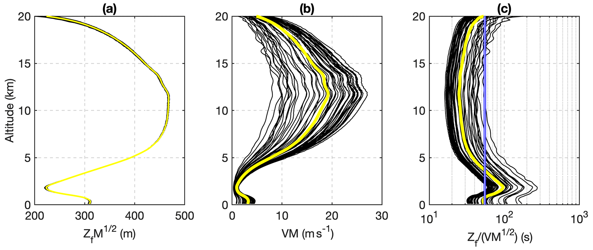
Figure 3(a) Diameter of the first Fresnel zone of the radio wave for BRO profiles from 12 December 2019. Thin black lines are individual BRO profiles, and the thick yellow curve is the daily mean for all panels. (b) Vertical velocity of the ray path tangent point during the occultation. (c) Time for the tangent point to cross the first Fresnel zone diameter as a function of height. The thin blue line indicates the selected window width (55 s) used to filter the excess Doppler.
During the first 17 d of the flight (6–22 December 2019) when a nearly continuous sequence of data were recovered, there were about 750 BRO profiles retrieved from the GPS satellites alone (top panel of Fig. 4). On average, there are 44 profiles retrieved per day. The sampling of the profiles is continuous in both time and space, in contrast to SRO, which has a quasi-random distribution. The balloon was floating predominantly eastward with an average velocity of 10–15 m s−1, at a time when the QBO was in the westerly phase of zonal-mean winds. The profiles were distributed in a band within ±10∘ of the Equator with an average separation of ∼100 km. The density of profiles over a given area varies with wind speed. The balloon path shows meridional motions associated with wave periods of ∼3–4 d. From 16–19 December 2019, the zonal wind was relatively weak, producing a very dense sampling of BRO profiles near 140∘ E longitude. The sampling was similarly dense between 9 and 14 January 2020 near −90∘ E longitude.
GPS satellites travel much faster (2000 m s−1) at much higher orbits (20 200 km ) than superpressure balloons floating with the wind at 20 km altitude. Over the duration of an occultation lasting about 10–20 min, the balloon is relatively stationary compared to the GPS satellite. For a setting occultation, the tangent points of the ray path descend and drift horizontally away from the balloon position as the satellite sets (blue lines in Fig. 4), and vice versa for rising occultations (red lines in Fig. 4). The slant profiles are aligned in four primary directions, roughly parallel to the orbital planes of the GPS satellites at the Equator (55∘ orbit inclination). Rising occultations on the north side of the balloon sample roughly from the NW to SE and on the south side sample from the SW to NE. Setting occultations sample from the SW to NE on the north side of the balloon and from the NW to SE on the south side of the balloon. The temporal sampling of tangent points in an individual profile always produces later sampling to the east. Within a short time window, four or more setting and rising profiles form a tetrahedral shape extending 500 km in four different directions. This nearly orthogonal distribution of BRO profiles is expected to present advantages for resolving wave structure in the horizontal direction. Multiple irregularly spaced but temporally and spatially consecutive profiles form near-parallel transects ∼400 km wide along the trajectory.
The spatial distribution of the 49 BRO profiles retrieved from GPS satellites on 12 December 2019 is shown in Fig. 5. There are 23 rising occultations (red) and 26 setting occultations (blue). The thick black line is the balloon flight track, and the balloon was flying eastward over Indonesia during that period. The profiles are relatively evenly distributed and continuous in both time and space, which provides a comprehensive sampling of the atmosphere beneath and surrounding the flight track. A typical BRO tangent point profile will drift as far as 500 km to the side of the flight path as the tangent point altitude decreases from balloon flight level down to 4–5 km altitude, producing the sequence of points appearing as curved lines in Fig. 5. The horizontal drift is greater at the top and varies slightly depending on the relative orientation of the satellite motion to the occultation plane. The horizontal drift is much larger than SRO over the same altitude range. For most occultations (41 out of 49), the lowest tangent point altitude reaches below 10 km, and the deepest profile reaches 4 km. Twenty-two SRO profiles from COSMIC-2 fell in the map area on that day. However, they are scattered randomly in both space and time, as shown in Fig. 5.
To evaluate the quality of the BRO observations, we compared them with observations from radiosonde launches when the balloon passed over the maritime continent. We also compared them with COSMIC-2 SRO profiles that were close in location and time and with reanalysis products from the European Centre for Medium-range Weather Forecasts (ECMWF) Reanalysis 5 (ERA5) (Hersbach et al., 2020). The hourly ERA5 reanalysis (European Centre for Medium-Range Weather Forecasts, 2019) interpolated from native model levels was chosen to represent the best estimate of the atmosphere state for this study, particularly for its high vertical resolution in the UTLS (∼300–400 m ) and high temporal resolution of 1 h. These ERA5 model level products have a horizontal resolution of (∼25–30 km) and 137 hybrid sigma-pressure levels in the vertical, up to a top level of 0.01 hPa. The geopotential and geometric height, as well as the pressure at each of the aforementioned model levels, were calculated using the method employed at the ECMWF (Simmons and Burridge, 1981; Trenberth et al., 1993). For each retrieved BRO profile, a corresponding refractivity profile from the ERA5 product was created by extracting the horizontal grid point closest to the observed tangent point for the nearest hour. Linear interpolation for temperature, specific humidity, and the logarithm of pressure was performed between the two nearest model levels in the reanalysis product to the height of the given tangent point in the BRO profile. Therefore, the final matching reanalysis profile also drifts horizontally and contains the same number of points as the given BRO profile. Note that the ERA5 products on pressure levels do not preserve sufficient vertical resolution to represent fine-vertical-scale waves.
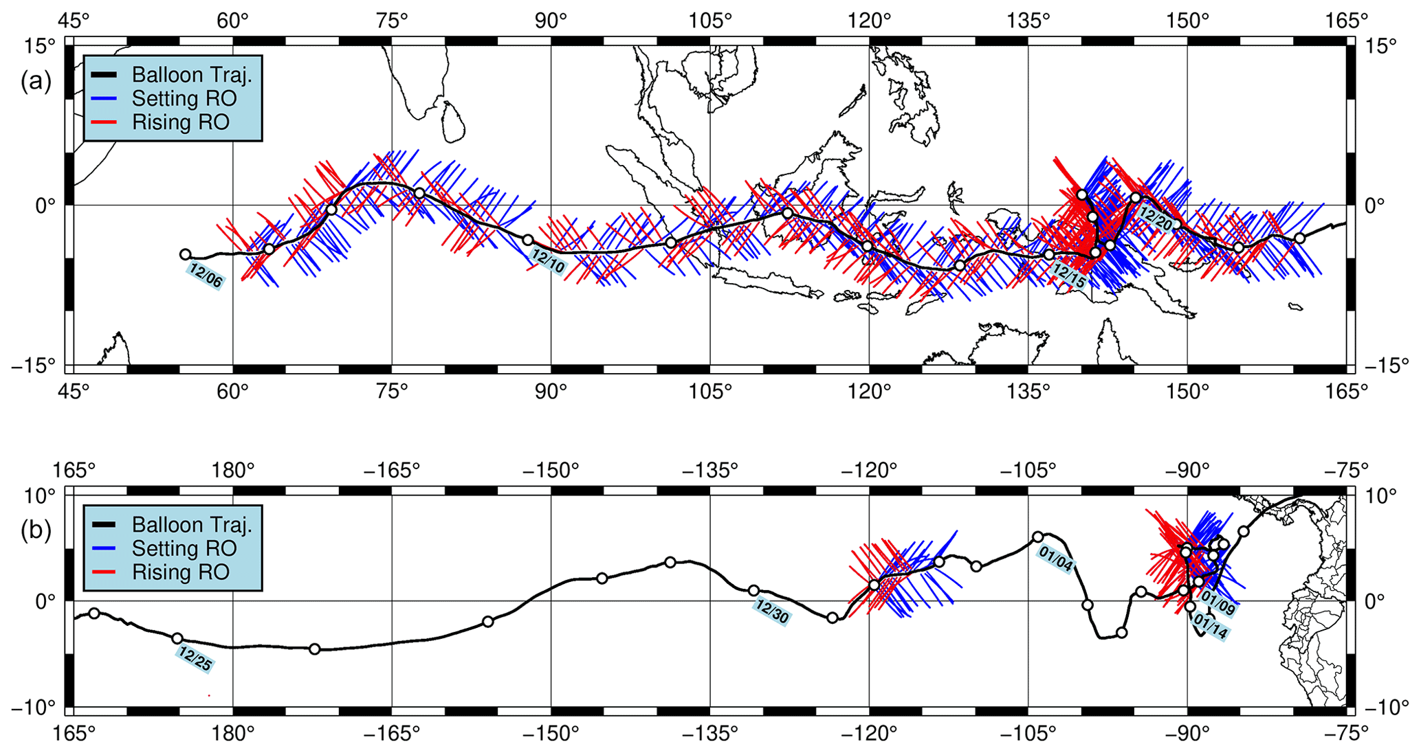
Figure 4Plan view of the slant BRO profiles from 6 to 22 December 2019 (a) and a few selected days in January 2020 (1, 9, 11, 12, 13) (b). The thick black line marks the trajectory of the balloon at the altitude of ∼20 km. Red and blue lines denote rising and setting BRO profiles, respectively, that are projections of slanted profiles with the highest tangent point on the balloon path and the lowest point furthest away. Small circles mark 00Z each day and are labeled with the date at 5 d intervals. Galileo and GLONASS data were recovered on 15 December and BeiDou data on 14 January but are not included in this map.
Figure 6a shows a BRO profile with the radiosonde observation at Mutiara SIS Al-Jufrie Airport near Palu, Indonesia (station ID 97092), and a COSMIC-2 RO profile (locations circled in Fig. 5). They were located about 300 and 150 km away from the BRO profile, respectively, and the time differences were less than 2 h. The refractivity profiles were calculated from the radiosonde and ERA5 products using Eq. (1) with water vapor pressure estimated from specific humidity (details in Appendix C). The matching ERA5 profile at the drifting tangent points is also shown in Fig. 6a. At each hour, we calculate the mean balloon location and then average all of the COSMIC-2 profiles that occur within ±15 d of that time and latitude and longitude of that location to construct a monthly mean background refractivity and temperature profile that captures synoptic-scale variations at periods much longer than the expected wave signatures. This COSMIC-2 “monthly mean” profile best represents the mean tropopause structure, excluding the influence of tropical waves. In Fig. 6b, the percentage refractivity difference relative to the monthly mean profile is shown. The observations all show similar deviations from the monthly mean climatology. The BRO, radiosonde, and COSMIC-2 profiles all contain small-scale wave features near and above the tropopause. The wave features are also present in ERA5, which assimilates both radiosonde and COSMIC-2 data. Visually, the BRO profile matches the ERA5 profile well, which we attribute to the fact that they both consider the same tangent point drift.
The refractivity differences between BRO and the radiosonde are ∼1 % from 4 to 15 km and ∼2 % above 15 km. Note that the radiosonde site is closer to the lower part of the BRO profile, as shown in Fig. 5, and the BRO profile is within an hour of the 00:00 UT launch time. Considering the spatial and temporal separation between the BRO and radiosonde measurements, the BRO profiles have an absolute accuracy better than 2 %. The temperature profiles (dry temperature for COSMIC-2 and BRO) are shown in Fig. 6c. The BRO dry temperature closely matches the radiosonde and COSMIC-2 temperature above 10 km and resolves the cold-point tropopause very well. Figure 6d shows wave temperature anomalies (absolute differences) from the COSMIC-2 monthly mean profile. A similar wave pattern can be identified in all observations, and waves are seen to sharpen and depress the cold-point tropopause temperature by ∼1 K, as has been observed in previous studies (Kim and Alexander, 2015). The differences in temperature between BRO, COSMIC-2, and the radiosonde are within 1 K above 10 km. Below 10 km, the BRO and COSMIC-2 profiles are similar as they both neglect water vapor and thus are not comparable to ERA5 and the radiosonde.
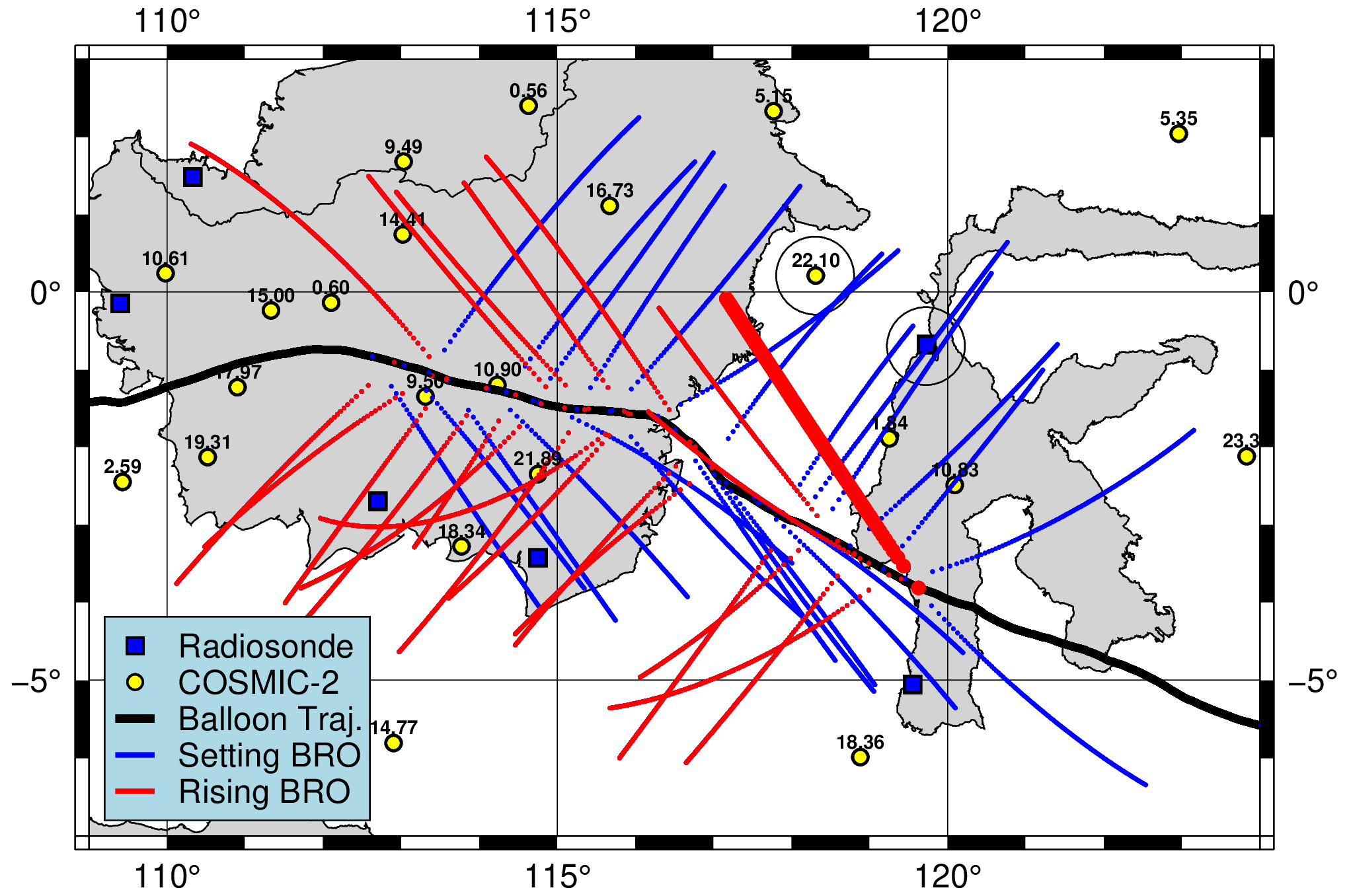
Figure 5Spatial distribution of the slant BRO profiles on 12 December 2019. The thick black line marks the balloon trajectory at the altitude of ∼20 km. Red and blue lines denote tangent point locations for rising and setting BRO profiles, respectively. Blue squares denote radiosonde stations, and yellow circles denote COSMIC-2 RO profile reference locations (neglecting the much smaller tangent point drift) over the same day. The numbers above the yellow circles are the time in hours of the COSMIC-2 RO profiles. The BRO profile denoted by a thick red line and the circled COSMIC-2 and radiosonde profiles are close in space and time and thus selected for comparison in Fig. 6. The transect of setting (blue) BRO profiles on the south side of the balloon trajectory is shown in Fig. 7. No COSMIC-2 RO profiles are obscured by the legend in the lower left corner.
The wave pattern observed in the radiosonde, COSMIC-2, and BRO profiles in Fig. 6 can be examined in more depth, given the large number of BRO profiles available. Figure 7 shows a series of 11 profiles that were collected consecutively in space and time from setting GPS satellites on the south side of the balloon track on the same day (12 December 2019), where the orientations of the tangent point drift were similar. The offsets between two adjacent profiles are proportional to the interval between them. The CPT is at ∼16 km and is associated with a vertical wave pattern that is common to all the profiles. This is even more clear when the large-scale background temperature profile is removed, shown in the lower part of Fig. 7. The background has its coldest point significantly higher, at about 17.5 km. This fine-vertical-scale (∼3–4 km wavelength) wave pattern seen in the BRO data must have a long intrinsic period (>1 d), since no obvious progression in phase is visible.
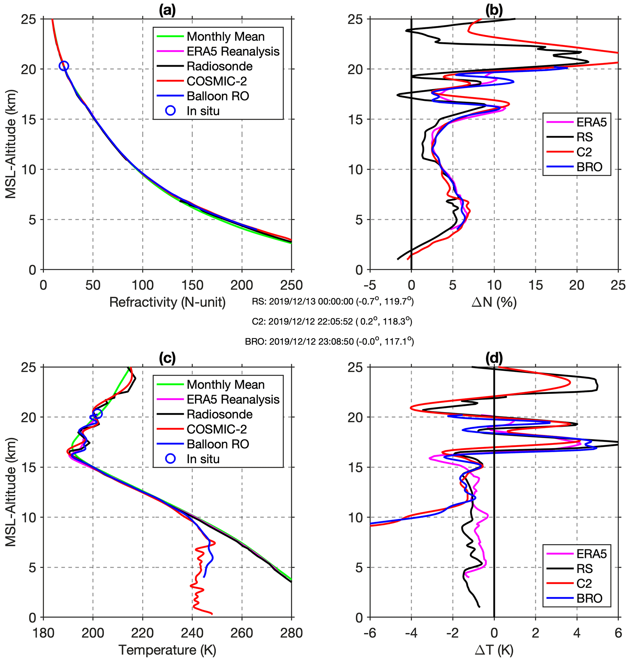
Figure 6(a) Refractivity profiles from BRO, the ERA5 reanalysis, a nearby radiosonde (RS), a COSMIC-2 RO profile (C2; locations shown in Fig. 5), and the monthly regional mean determined from COSMIC-2. (b) Percentage refractivity differences of ERA5, radiosonde, COSMIC-2, and BRO with respect to the COSMIC-2 monthly mean. (c) Corresponding temperature (dry temperature for COSMIC-2 and BRO) profiles. (d) Corresponding temperature differences with respect to the COSMIC-2 monthly mean. The time and location of the radiosonde, COSMIC-2 RO, and BRO are listed in the panel (year/month/day hh:mm:ss UT (lat, long)).
A statistical comparison between BRO and the corresponding ERA5 reanalysis profiles for the entire 17 d period is shown in Fig. 8. The number of points from the BRO profiles at each height is indicated in black lines. The lowest tangent point altitude in each profile varies because the PLL receiver loses or initiates tracking of different satellites at different altitudes. Most of the profiles (∼600) penetrate below 10 km, and ∼400 profiles penetrate below 8 km. The differences are characterized by the mean and standard deviation (SD) of the absolute and percentage differences between the two datasets. The mean difference between BRO refractivity and ERA5 is within 0.1 N-units, and the corresponding percentage difference is about 0.2 % above 7 km. The mean difference between retrieved dry temperature and ERA5 is within 0.5 K above 11 km, where moisture is negligible, with BRO showing higher temperatures. A residual wave-like pattern is apparent in the differences above 15 km, which is likely the signature of a large-scale and slowly varying wave captured by BRO that is coherent over the 17 d and is not captured accurately or is underrepresented in ERA5, as seen in Figs. 6c and 7. Because the dataset extends only ∼100∘ in longitude along the Equator, the large-scale wave perturbations were not averaged out and are still evident in the BRO dataset.
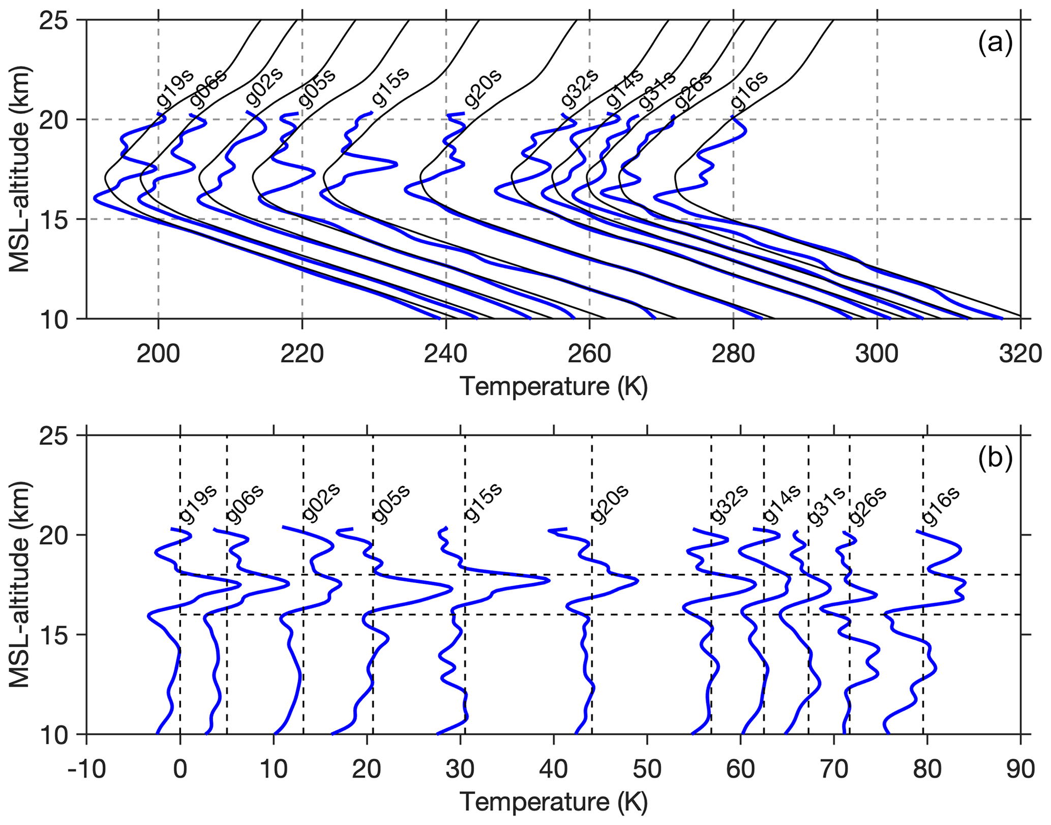
Figure 7(a) Transect of northwest–southeast-oriented BRO temperature profiles (blue lines) from 12 December 2019 south of the balloon trajectory (see Fig. 5; blue lines) ordered by time; the offsets are proportional to the intervals. COSMIC-2 background profiles are shown as black lines. (b) BRO profiles with the background removed. A coherent wave structure with ∼4 km wavelength dominates the variability.
Although there are many COSMIC-2 profiles over the equatorial region during the period of the Strateole-2 campaign, the number of profiles available to implement a profile-to-profile comparison between the two datasets is quite small. To compare the two types of RO profile, the daily mean refractivity and temperature were calculated for each dataset by averaging all RO profiles that occurred over a day within a box of 10∘ latitude by 10∘ longitude centered on the mean balloon position for the day. There were typically about 15–25 COSMIC-2 profiles per day falling in such an area compared to ∼45 BRO profiles. There are in total 17 daily mean profiles calculated for both RO datasets. Figure 9 shows the absolute and percentage differences in daily mean refractivity between BRO and COSMIC-2. There is a ∼0.1 N-unit mean difference between the two datasets above 15 km, corresponding to a 0.2 % difference. The mean temperature difference is within ∼0.5 K between two RO datasets above 8 km, with BRO showing higher temperatures. The largest differences at 17 km altitude close to the tropopause suggest that the COSMIC-2 daily mean may not capture all of the wave structure present in the higher-vertical-resolution BRO observations. Residual wave effects may also be associated with the limited sampling of COSMIC-2 or the latitudinal dependence of waves that may result in averaging out some variability. The technique for constructing composites of COSMIC-2 data is explored further in Sect. 6. Between 7–15 km, the differences are very small and stay within 0.1 % of the refractivity. The BRO observations are expected to be noisier than COSMIC-2 RO near the top of the profile because the accumulated bending angle along the ray path and the excess Doppler are small compared to velocity errors from the position uncertainty (Muradyan et al., 2011). However, the in situ refractivity observations assure the errors are small. The comparison between the two datasets illustrates that the same technique on different platforms can consistently observe large-scale atmospheric properties. The difference seen in the dry temperature below 15 km might be due to the different numerical schemes of calculating the dry temperature in the two datasets.
A primary objective of this work is to determine the properties of the equatorial waves that are evident in the BRO dataset, such as in the data presented in Fig. 7. The TSEN instrumentation on the Euros gondola measures flight level temperature and horizontal wind from the balloon position and reveals some properties of the wave spectrum. The Lagrangian frame of reference on the floating balloon enables a direct measurement of intrinsic wave frequencies. From these measurements, we compute the wave energy spectrum as a function of intrinsic frequency over the 57 d flight, which contains the period of high-density BRO measurements. Figure 10 shows the spectrum for waves with periods of 1–30 d. The spectrum shows a main peak near 20 d and secondary peaks at 3–4 d plus a background of higher-frequency waves. The 20 d signal is associated with a large quadrature in zonal wind and temperature without any coherent meridional wind signal (not shown), permitting interpretation of the 20 d signal as a Kelvin wave. The clear break in the spectrum near 5 d is next selected as the cutoff period for filtering to separate this Kelvin wave from shorter-period waves in BRO temperature profiles.
Given the characteristics of the profile transects shown in Fig. 7, we investigated the ability of BRO profiles to capture the properties of equatorial waves with short vertical wavelengths. In order to extract the wave components, background temperature profiles were subtracted from each BRO profile. The background temperature is defined as the moving average of all COSMIC-2 profiles that occurred within ±15 d and ±2∘ latitude and ±10∘ longitude surrounding the balloon location. Temperature perturbations thus include waves with periods shorter than 30 d. The BRO temperature perturbation profiles in Fig. 11a are ordered in time along the balloon track, with the corresponding longitudes shown on the top axis. The altitude of the BRO cold-point tropopause (CPT) is also shown in Fig. 11a. The coherent descent of phase with time, characteristic of upwardly propagating tropical wave energy, is observed in the stratosphere, as well as variability on a wide range of timescales. The longer-period coherent wave is clear in the BRO profiles that are filtered within periods of 5–30 d shown in Fig. 11c.

Figure 8(a) Absolute refractivity difference between BRO and ERA5 (BRO minus ERA5), (b) percentage refractivity difference, and (c) absolute temperature difference. Solid and dashed blue lines are the mean and standard derivation (SD) of the differences between the two datasets. Note that the true temperature is shown for ERA5 and the dry temperature is shown for BRO. The number of BRO measurements at each altitude is shown by the black line and top axis. For reference, the vertical dotted lines around zero represent 0.1 N-units and 0.2 % in absolute and percentage differences and 0.5 K in temperature difference.
Figure 11b shows the residual temperature variation after removing the dominant long-period signal from Kelvin waves (5–30 d period) shown in Fig. 11c. This isolates the tropical wave variability at periods ≤5 d. These shorter-period wave signals commonly reach ±4 K, and coherent phase descent is evident at times. Variability at the shortest timescales may be convolved with spatial wave variability, and multiple waves may be present, so further study of these high frequencies will be the subject of future work. Previous analyses of ground-based tropical observations at fixed locations have chosen a cutoff period at ≤3 d to isolate inertia–gravity waves (Sato and Dunkerton, 1997). Pass bands of ≥4–7 d periods have been used to isolate Kelvin waves (Tsuda et al., 1994; Kiladis et al., 2009). However, these analyses were performed in a ground-based reference frame, while we observe in a Lagrangian frame and at latitudes very close to the Equator. This frame-of-reference difference is an important distinction, and we will show clear differences in waves observed in these two frames of reference in what follows. While mixed Rossby–gravity waves and Kelvin waves can occur near a 5 d intrinsic period, we do not observe these signals around this period of high-density BRO data.
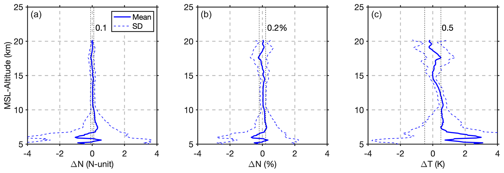
Figure 9(a) Absolute refractivity difference between daily mean BRO and daily mean COSMIC-2 RO (BRO minus COSMIC-2), (b) percentage refractivity difference, and (c) dry-temperature difference. The COSMIC-2 profiles are within 10∘ latitude and 10∘ longitude of the daily mean balloon position. Vertical dotted lines around zero represent 0.1 N-units and 0.2 % in absolute and percentage difference and 0.5 K in dry temperature.
Figure 11c shows the filtered temperature perturbation within the period band of 5–30 d, which contains Kelvin waves with a peak period of ∼20 d. The vertical structure of the 5–30 d signal in the stratosphere (Fig. 11c) has a dominant vertical wavelength of ∼6 km until day 350. Then after day 352, a ∼3 km vertical wavelength signal is more prominent. We can estimate the horizontal wavelength using the dispersion relation for Kelvin waves:
where is intrinsic frequency; N is buoyancy frequency (∼0.025 rad s−1); and k and m are the horizontal and vertical wavenumber, respectively. The 6 km signal is thus associated with the zonal wavenumber (wn)-1 Kelvin wave and the 3 km signal with wn 2.
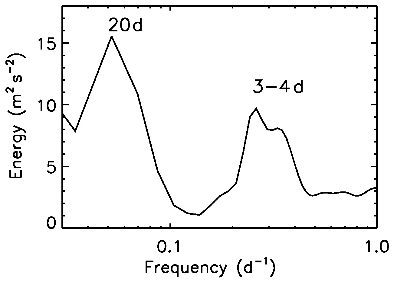
Figure 10Intrinsic frequency spectrum of total wave energy (m2 s−2) from TSEN measurements at the balloon float altitude near 20 km for the flight containing the time of the high-density BRO measurements.
A comparable estimate of the 5–30 d period Kelvin wave perturbations observed by COSMIC-2 is demonstrated by constructing composite temperature profiles following the balloon trajectory. These profiles were obtained by averaging the COSMIC-2 profiles that occurred within ±12 h and ±2∘ latitude and ±10∘ longitude of the hourly mean balloon location. Then, the same previously defined monthly mean background was removed from these profiles. The residual temperature perturbations are shown in Fig. 11d. The pattern is very similar in the BRO and COSMIC-2 observations, but the amplitudes in BRO appear stronger, particularly in the later period where the 3 km vertical wavelength structure dominates. The larger amplitude of the Kelvin wave signal in the BRO data can be explained by the higher vertical resolution of BRO compared to SRO derived in Sect. 4.2. Figure 12 shows this more quantitatively by comparing profiles in Fig. 11c and d on days 346 (when the 6 km wavelength signal dominates) and 353 (when the 3 km wavelength signal dominates). The same Kelvin waves are well observed by both datasets; however, the ones observed by COSMIC-2 show amplitudes attenuated by ∼20 % compared to BRO. The discrepancies below 15 km might be due to different numerical schemes of calculating the dry temperature from refractivity, which can also be seen in Fig. 9c.
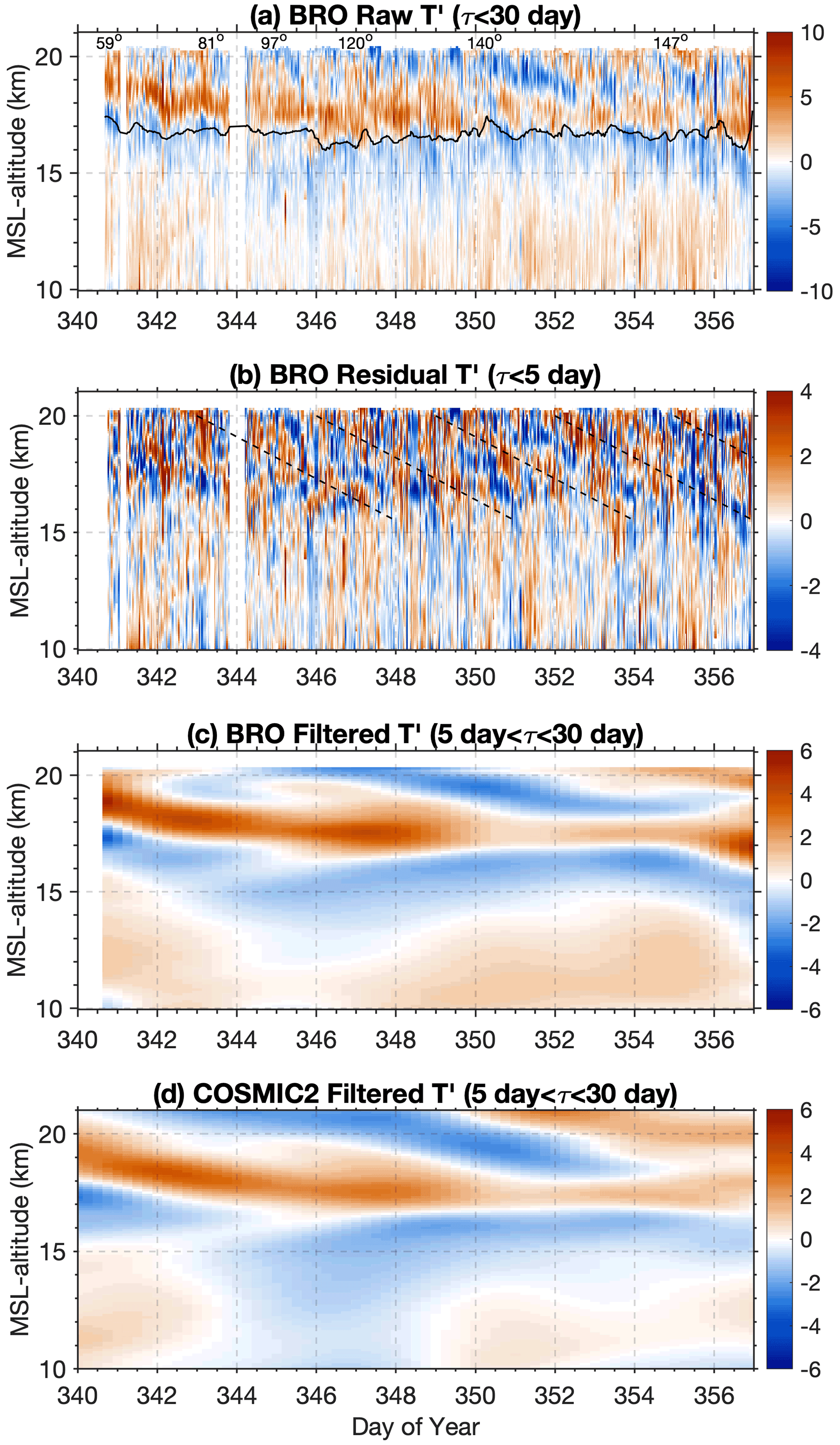
Figure 11Time–altitude cross-section of the 17 d continuous measurement period. (a) BRO temperature perturbations with periods of less than 30 d, (b) BRO temperature perturbations with periods of less than 5 d after removal of Kelvin waves, (c) BRO Kelvin wave perturbations (periods in the band 5–30 d), (d) COSMIC-2 Kelvin wave perturbations (5–30 d) from composite profiles. The black line in (a) marks the cold-point tropopause height. Numbers on the top axis of (a) are the longitudes at the corresponding time.
To illustrate the effect of the balloon's Lagrangian frame of reference on wave observations, Fig. 13 shows temperature perturbations in the ground-based frame of reference. In panel (a), the COSMIC-2 data shown are from the daily average of temperature profiles within a fixed area (a box from 2∘ S–2∘ N and 120–140∘ E), band-pass filtered between 5 and 30 d. In panel (b), radiosonde data from Manado, Indonesia (station 97014; 1.53∘ N, 124.91∘ E) are high-pass filtered for periods shorter than 5 d. Both datasets are organized by altitude and time for comparison with the BRO dataset, filtered for the same periods. Unlike the BRO dataset in the Lagrangian frame, as shown in Fig. 11, the filtered COSMIC-2 temperature perturbations within periods of 5–30 d (Kelvin wave signal) show different features. Figure 13a shows a relatively steady downward progression of phase in time in this ground-based frame. During days 340–350, the period of the wn-1 Kelvin wave observed in this frame is closer to 16 d, shorter than the 20 d observed in the TSEN data. This intrinsic period could also be resolved by BRO data given that more data were retrieved.
Linear wave theory predicts that the difference between ground-based frequency and intrinsic frequency is equal to the zonal-mean QBO wind (U) times wavenumber k:
The difference is therefore consistent with an eastward mean wind of U∼8 m s−1, a value closely matching the observed zonal wind. In the Lagrangian frame, the balloon moves faster during the eastward Kelvin wave phase. During the westward phase of the Kelvin wave, the balloon slows considerably, but during part of that time it is still moving eastward. Thus when the balloon and wave move in the same direction and the wave propagation is faster than the mean wind, the balloon spends more time in eastward motion and less time in westward motion. This difference would be reversed if the QBO were in the westward phase.

Figure 12Profiles of Kelvin wave temperature perturbations from COSMIC-2 and BRO from Fig. 11c and d, on (a) day 346 when the 6 km vertical wavelength dominates and (b) day 353 when the 3 km wavelength dominates.
Here we use two methods to make a rough estimate of momentum flux, one relying primarily on temperature perturbations from BRO data and one relying primarily on TSEN data. As presented in the Appendix of Ern and Preusse (2009), the gravity and Kelvin wave momentum fluxes can be estimated from relative temperature perturbations with known intrinsic wave frequency, vertical and zonal wavenumbers, atmospheric density, and buoyancy frequency.
in which ρ0 is the atmospheric density, is the background temperature, and N2 is the squared buoyancy frequency. These formulas were applied to SABER (Ern and Preusse, 2009) and HIRDLS (Alexander and Ortland, 2010) observations and also SRO datasets, such as COSMIC-1 (Schmidt et al., 2016). With BRO data retrieved in the Lagrangian framework and better resolution of the wave amplitudes, a more accurate estimate of the wave momentum flux could be achieved near the balloon flight altitude. Assuming a background temperature of 195 K, a density of ∼0.1 kg m−3, and a buoyancy frequency of 0.025 rad s−1 at about 20 km, the momentum fluxes of the Kelvin waves with wn 1 and wn 2 are estimated to be around 0.15 and 0.09 mPa, respectively. These values are reasonable and, for example, within the range of values deduced from radiosonde data in Sato and Dunkerton (1997, their Fig. 7) during the westerly phase of the QBO, which was about 0.1–0.2 mPa at around 20 km.
Sato and Dunkerton (1997) provide a different way of estimating the Kelvin wave momentum flux by relating it to the quadrature spectra of temperature and zonal wind perturbations.
where is the quadrature spectra of the temperature and zonal wind fluctuations at intrinsic frequency . This is a direct estimation of total momentum flux that contains both positive and negative momentum flux. The quadrature spectra of temperature and zonal wind perturbations were calculated from the TSEN measurements; a peak of about −3 K m s−1 was found for the 20 d Kelvin wave around the BRO high-density observation period (not shown). Using the same constants as defined above, the total momentum flux associated with the Kelvin wave is calculated to be around 0.09 mPa. This value is slightly smaller than the ones estimated from the BRO temperature measurements.
Figure 13b shows the high-pass-filtered (5 d cutoff period) radiosonde temperature anomalies. Again differences between perturbations in this ground-based reference frame and in the Lagrangian frame (Fig. 11b) are apparent, but with many different frequencies and wavenumbers of gravity waves likely contributing to these perturbations, interpretation is more complex and left to future work.
We have shown the level of consistency of the BRO observations with radiosonde observations and made statistical comparisons with the ERA5 reanalysis and COSMIC-2 RO for the larger-horizontal-scale Kelvin waves, providing confidence in the information extracted from the BRO observations. The RO technology has been deployed on many satellite missions to provide datasets with global coverage, either as a primary payload in dedicated constellations or as a secondary payload in other science missions and recently in commercial CubeSat constellations. The BRO observations extend the general capabilities of GNSS RO to dense consecutive profiles that can be exploited to investigate coherent finer-vertical-scale wave variability, as illustrated above. There is a rich dataset still to be explored in terms of three-dimensional propagation characteristics and directionality by analyzing transects with different orientations from the orthogonal pattern of tangent point profiles. These capabilities will be further enriched by recovering data from multiple constellations, including Galileo, GLONASS, and BeiDou. A 24 h dataset was retrieved from the Galileo and GLONASS constellations that was sufficient to demonstrate quality comparable to GPS. A 12 h dataset was retrieved from BeiDou. Due to data transmission limitations, however, it was not possible to transmit the additional constellation datasets from the entire flight. The data were sufficient to verify the number of occultations from each constellation. On average, there were approximately two profiles retrieved per hour from the GPS constellation. Including data from all GNSS constellations more than doubles the number of profiles. The multi-constellation recordings that were successfully tested for 1 d during this campaign are planned to be implemented for future Strateole-2 science campaigns, which will have increased communication bandwidth. Multi-constellation recordings will further improve spatial and temporal resolution.
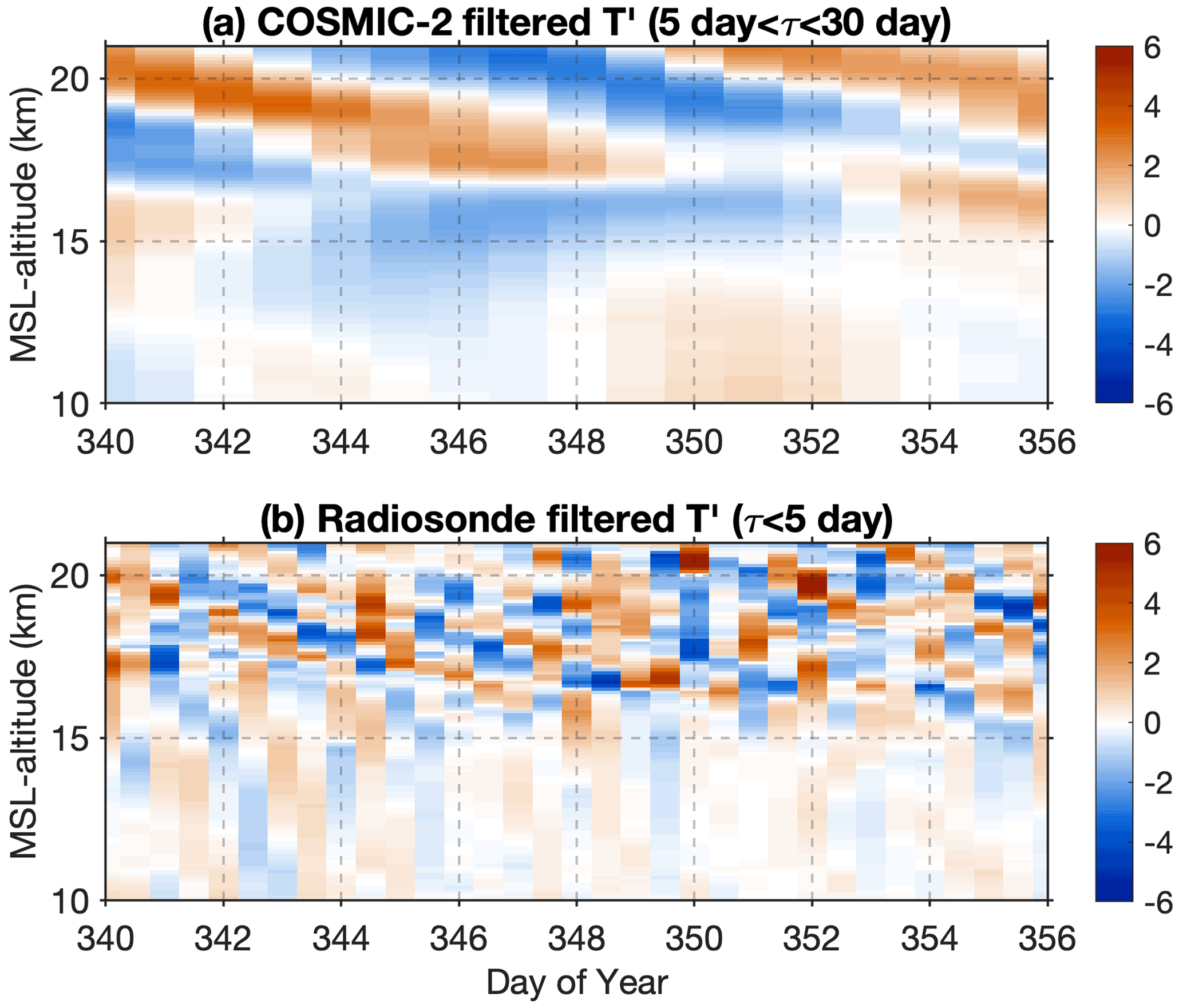
Figure 13(a) Time–altitude cross-section of COSMIC-2 temperature perturbations binned at a fixed location surrounding the radiosonde site (2∘ S–2∘ N, 120–140∘ E) and band-pass filtered at a 5–30 d period. Time is indicated with daily values at 12:00 UT on the horizontal axis. (b) Radiosonde (1.53∘ N, 124.91∘ E; station ID 97014) temperature perturbations high-pass filtered for periods shorter than 5 d. Time is indicated with daily values at 00:00 and 12:00 UT on the horizontal axis.
The BRO observations of temperature variability in a moving reference frame provide a unique benefit when interpreting wave characteristics from dispersion relations. Strictly speaking, the dispersion relations that relate the intrinsic period to wave speed hold in the intrinsic (Lagrangian) reference frame. Infrared satellite data that are often used to capture wave modulation of deep convection (i.e., Kiladis et al., 2009) are typically displayed and analyzed in an Earth-fixed (i.e., ground-based) reference frame. In the troposphere, where the winds are weaker and more random, the approximation that the reference frames are nearly equivalent has a negligible effect. However, in the stratosphere, where the mean flow is stronger, the wave dispersion curve in the intrinsic Lagrangian reference frame (i.e., the wave speeds) is different from the ground-based reference frame. This can be seen clearly in Fig. 13a where the COSMIC-2 profiles are averaged over boxes in a ground-based reference frame, in comparison to a reference frame that moves with the balloon in Fig. 11d. The latter appears quite similar to the BRO profiles. In fact, the period estimated for the former is closer to 16 d, whereas the intrinsic period observed by BRO is closer to 20 d. Often the dispersion curves calculated in the Lagrangian reference frame for different wave types are shown on the same diagrams with satellite-derived observations in the Earth-fixed reference frame (i.e., Kiladis et al., 2009), without accounting for these differences. Similarly, the difference is also highlighted in the shorter-period perturbations from BRO in Fig. 11b where waves with an intrinsic period of 3–4 d are present. The radiosonde data in the ground-based reference frame in Fig. 13b may capture the same waves but at different intrinsic periods. This is further complicated due to the likelihood that the data contain many wave types. The intrinsic period and wave speed can be significantly different, also affecting any estimates of momentum flux. The wave analysis is based on dry-temperature profiles above 10 km, using the retrieval method based on the assumptions of negligible water vapor and hydrostatic equilibrium (Kursinski et al., 1997). As expected, there is a deviation of dry temperature from the true temperature at lower altitudes. With prior information (a first guess) from the model about the temperature and water vapor pressure and their uncertainties, the temperature and moisture information could potentially be retrieved using the 1D-Var methodology (Poli et al., 2002), for example, as implemented in the COSMIC Data Analysis and Archive Center (CDAAC) (COSMIC Project Office, 2005). However, as seen in Fig. 6, this would involve a more complicated interpretation of the wave structure in the altitudes of interest when the background or first-guess model has a significantly different vertical structure, so it is not used here.
Very high accuracy positioning is required for balloon-borne RO observations because of the sensitivity to Doppler velocity errors. The higher-accuracy positioning yields an additional benefit relative to the single-frequency GNSS receiver in the standard TSEN sensor package provided for all deployed balloons. This precise positioning provides better estimates of the winds and reliable vertical positions that are independent of the pressure measurement, which makes it possible to resolve the Eulerian pressure independently of altitude for the intrinsic phase speed estimation in the spectral analysis of the in situ data (Boccara et al., 2008; Vincent and Hertzog, 2014). This was illustrated in the high-precision positioning used in the gravity wave analysis of the stratospheric balloon data from the Antarctic Concordiasi campaign and led to better estimates of the momentum flux of high-frequency gravity waves (Zhang et al., 2016). A similar analysis is planned for future Strateole-2 observations.
The COSMIC-2 constellation provides profiles over the tropical oceans operationally for assimilation into numerical weather prediction models and achieves a median latency of 30 min (Weiss et al., 2022). The increased density of the Strateole-2 observations provides potential added value for models, and the processing scheme is quite similar. The observations are transmitted via an Iridium satellite communication link at 1 h intervals, so there could be as much as 30 min of additional median delay, which would still be of potential value for numerical weather prediction (NWP). Efforts are underway to develop low-latency products for aircraft RO observations. Implementing the same techniques for near-real-time balloon observations could contribute to improving model initial conditions over the tropical oceans in future campaigns.
This work is the culmination of efforts to design and deploy the second-generation Global Navigation Satellite System (GNSS) Radio OCcultation (ROC) receiver on board equatorial long-duration stratospheric balloons. The Strateole-2 technology demonstration campaign in 2019–2020 was the first time that balloon-borne GNSS RO was used to derive high-vertical-resolution equatorial wave observations. About 45 temperature profiles were retrieved daily over a period of 17 d, from ∼20 km down to a median altitude of 8 km. The BRO technique samples the atmosphere in an orthogonal pattern over a broad area (±400–500 km) along both sides of the flight track, which will be helpful in the future for examining horizontal variations in wave propagation characteristics.
For verification, retrieved refractivity and dry-temperature profiles were compared with co-located radiosonde observations over Indonesia within 300 km and 1 h of the observation time. The BRO refractivity profiles show good agreement with radiosondes, given the large horizontal drift of the profile tangent points, within 2 % refractivity and 1 K temperature from flight level to 10 km altitude. Most importantly, the BRO profiles, with vertical resolution better than 500 m, show the same vertical wave structure in the temperature and wave-generated depression of the cold-point tropopause as is seen in the radiosonde profiles. Over the duration of the flight over the maritime continent, the mean difference with the ERA5 reanalysis is less than 0.2 % refractivity above 7 km, and the standard deviation is less than 1 %. A systematic bias in comparison with ERA5 from 15 to 20 km is explained by a large-scale Kelvin wave observed in the data that is not adequately resolved or represented in the ERA5 reanalysis. We computed the daily regional mean from the much sparser COSMIC-2 RO profiles to compare them to the daily mean BRO profiles and found excellent agreement from balloon flight level down to 8 km altitude, with an rms difference of less than 0.1 % refractivity. Slightly larger differences at 17–18 km are a possible indication that wave variations with a less than 3 km wavelength are not resolved in the sparser spaceborne RO dataset.
The dominant signal in the individual BRO profile transects, made visible by the consecutive sampling in time and space, is a large-scale Kelvin wave with a ∼3–6 km vertical wavelength. The same Kelvin wave is also visible in the COSMIC-2 data, when a new approach is used to bin the COSMIC-2 data following the balloon trajectory, essentially mapping the COSMIC-2 observations into the intrinsic reference frame. However, the BRO observations with slightly higher vertical resolution and denser sampling retrieved as much as 20 % higher amplitude temperature variation associated with the wave. The BRO observations present the advantage that the waves are naturally measured in the intrinsic reference frame. The BRO profiles show an intrinsic period of 20 d for the Kelvin wave as compared to 16 d period for the Kelvin wave in the ground-referenced COSMIC-2 dataset. The difference in wave amplitudes and wave periods determined from the BRO-vs.-COSMIC-2 datasets affects the calculation of momentum flux. After removing the large-scale signal of the Kelvin wave, the BRO observations show wave variations with a 2–3 km vertical wavelength that are interpreted to be westward-propagating inertia–gravity waves with a 3–4 d period. These results demonstrate the ability to extract fine-vertical-scale wave properties continuously in time and space in poorly sampled regions of the globe. The results are promising and indicate that the data will be useful for distinguishing contributions that waves of different scales make to momentum forces for wave driving of the QBO, which is expected to lead to improved QBO representation in models.
We retrieved a small dataset from the Galileo and GLONASS constellations, which have comparable accuracy to GPS, and demonstrated the feasibility to nearly double the sampling density. Experimental data from the BeiDou constellation were also collected. Five balloons carrying the ROC receiver will be deployed to perform RO observations in a follow-on campaign. Improved Iridium data rates are expected to be high enough to support the continuous transmission of all constellations throughout the entire flight. Exploiting the full dataset and the information available from the directional sampling of the profiles on the north and south sides of the balloon paths will provide opportunities to capture waves over an even broader range of scales.
BRO observations contribute to the larger objectives of the Strateole-2 campaigns that include multiple types of instruments to be flown in the coming years. The high-vertical-resolution dataset provides new knowledge on fine-vertical-scale waves that are unresolved in global models and provides direct observations of their spatial structure. When combined with other observations, such as the BeCOOL micro-lidar nadir cloud observations, the BRO observations will help determine the relationship of upper-troposphere waves to the presence of cirrus clouds that can be used for improving model representations of these clouds. They will help quantify global characteristics of waves that determine cold-point tropopause temperature variability for use in improving models of stratospheric dehydration. Slow upwelling, rapid transport by penetrating deep convection, thin cirrus formation, and horizontal transport and cooling by waves combine to give the observed variability in water vapor on timescales ranging from very short to decadal. Because stratospheric water vapor plays an important role in the radiative budget of the stratosphere as well as in modulating surface warming, quantifying wave properties in the equatorial region that modulate the transport of moisture from the troposphere is essential for improving climate models.
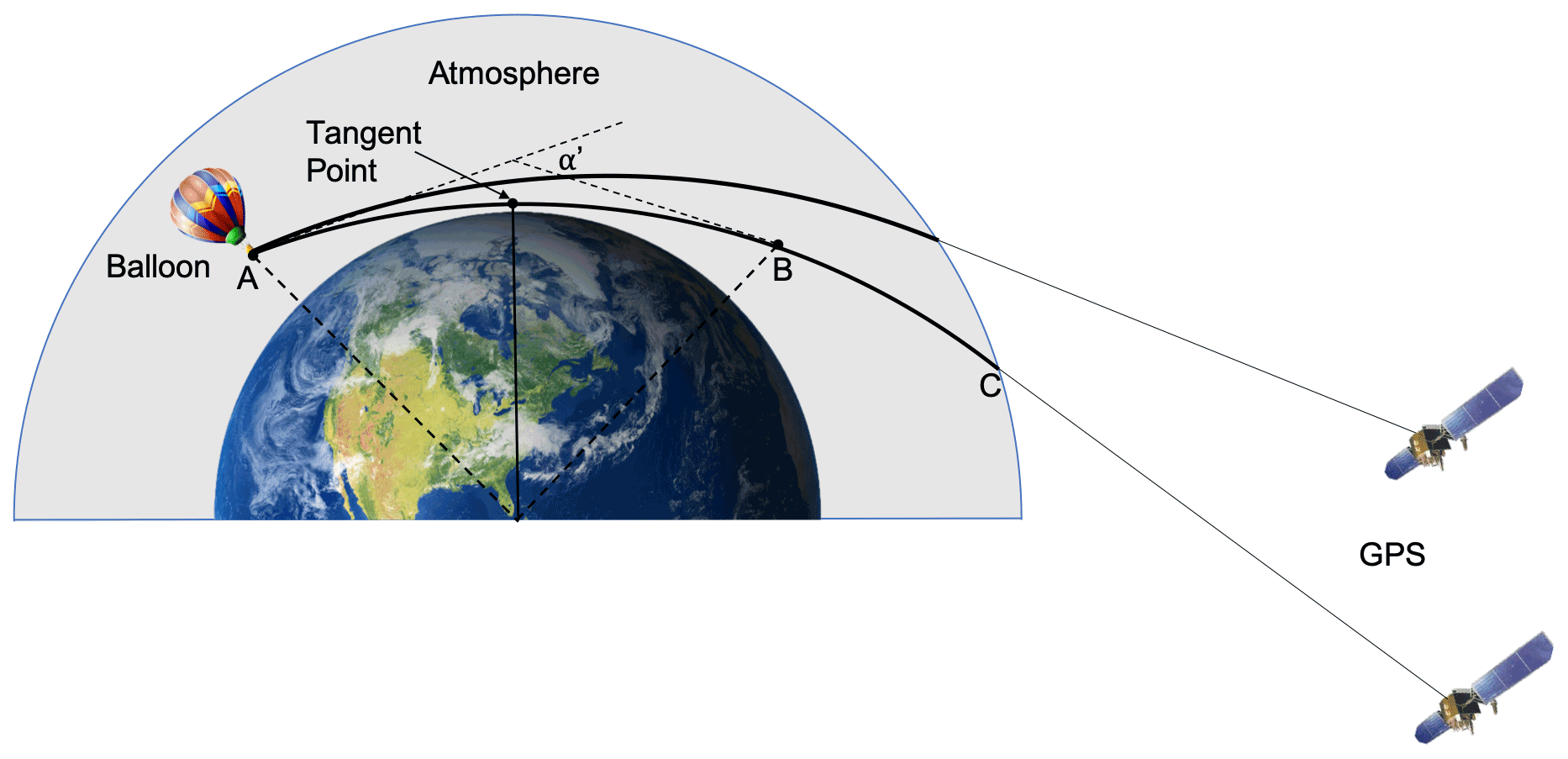
Figure A1Schematic diagram of balloon-borne RO geometry with a receiver inside a spherically symmetric atmosphere (shaded). The solid lines connecting the balloon and the GPS satellites represent ray paths of the navigational signal at different times, with thicker parts within the neutral atmosphere. Point B on the ray path is symmetric with respect to the tangent point to balloon position A. The bending angle α′ is the partial bending angle that accounts only for the bending of the ray path segment AB. Note that the schematic figure is not to scale and the ray path bending is exaggerated for the purpose of visualization and is less than 2∘.
The BRO geometry is similar to that of SRO except that the receiver is within the neutral atmosphere, as shown in Fig. A1. The excess phase delay is defined as the difference between the observed propagation time of the signal from the satellite to the receiver and the travel time in a vacuum, multiplied by the speed of light. The excess phase is the integral along the ray path of the refractive index. It is the fundamental observed quantity, expressed in distance units as the carrier-phase cycles multiplied by the speed of light, and is typically as much as 100–200 m for BRO. The derivative of the excess phase with time is the excess Doppler shift in the GNSS transmitter carrier frequency, for convenience, given in units of speed (m s−1). In a spherically symmetric atmosphere, the ray path bending angle can be derived from the excess Doppler shift (Hajj et al., 2002; Kursinski et al., 1997) using an iterative method, geometric constraints, and Bouguer's law for optical refraction (Born and Wolf, 1999; Vorobév and Krasilńikova, 1994):
Here the impact parameter, a, is constant for a given ray path, and ϕ is the angle between the radius vector, r, and the ray path tangent vector. rT and rR refer to the radius vectors of the satellite transmitter and receiver positions, respectively, and rt is the radius at the tangent point. The result is an estimate of the bending angle as a function of ray impact parameter a. The accuracy of the bending angle derived from the excess Doppler is subject to the accuracy of the velocity of the transmitter and receiver (Xie et al., 2008; Muradyan, 2012; Muradyan et al., 2011).
Theoretically, the ray path bending is also described by an integral over radius r from the receiver altitude to the altitude of the tangent point and then to the GPS satellite altitude, in the case of a spherically symmetric atmosphere:
The receiver is low enough that it cannot be considered to be in a vacuum, so the asymmetric geometry requires a correction for the in situ refractivity. It also requires a correction for the refractivity above the receiver for the positive elevation angle segment of the ray path from point B to C in Fig. A1. The partial bending angle is defined as the difference between the total bending accumulated for the ray path arriving at the receiver from an elevation angle below the horizon (negative elevation angle) minus the positive elevation angle bending (Xie et al., 2008). It corresponds to the accumulated bending from the segment of the ray path below the altitude of the receiver, which is the first term on the right side of Eq. (A2). In Fig. A1, this segment of the ray path is between point A and point B, which is symmetric with respect to the tangent point. The partial bending angle α′ is then inverted using the Abel transform to retrieve the refractive index profile.
nR is the refractive index at the receiver altitude and is determined by in situ measurements from meteorological sensors on board the same balloon. Finally, the refractive index profile as a function of altitude n(h) is retrieved using the relation , where RE is the local radius of curvature of the ellipsoidal Earth and h is the altitude above the ellipsoid.
For each balloon-borne RO profile, the retrieved refractivity is derived from an integrated measurement along the ray path, whose effects are represented as a localized value at the tangent point. One way to define the horizontal resolution is to use the length of the ray path centered at the tangent point that contributes 50 % of the excess phase or bending. Using ray tracing, we simulated the GNSS signal propagation in the atmosphere for one setting occultation near the Equator. Figure B1a shows the ray paths projected to a horizontal map view, and Fig. B1b shows a vertical cross-section for the segments of the ray paths that traverse the atmosphere below the height of the balloon at 20 km. The thicker segments on the ray path surrounding the tangent points account for 50 % of the total excess phase. The time interval between each ray path shown in panel (b) is 150 s. The horizontal drift of the tangent points (red dots) is clearly seen in these two panels. At this scale, the motion of the balloon during the ∼25 min occultation is imperceptible. The horizontal distance ΔL and corresponding altitude range Δz of this segment provide one way of defining the resolution. In Fig. B1c, ΔL varies from ∼275 at 10 km height to 170 km at the tropopause at ∼18 km as Δz varies from ∼1.4 to 0.7 km in Fig. B1d.
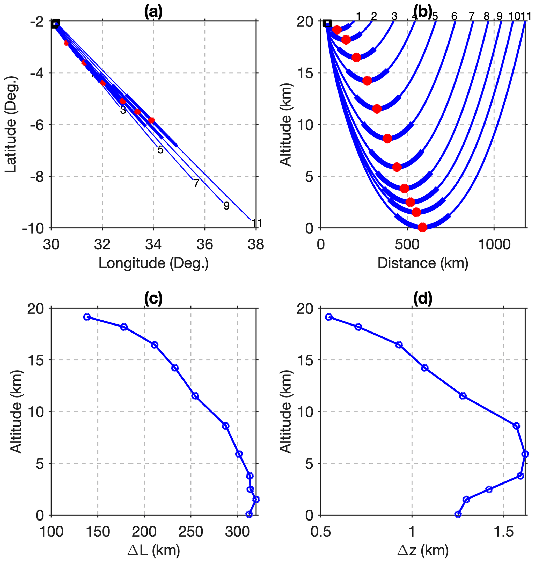
Figure B1The signal ray paths of one setting occultation in the (a) horizontal plan view and (b) vertical cross-section view. The numbers label the ray path traversing the atmosphere from top to bottom with 300 and 150 s intervals for (a) and (b). The black square marks the position of the balloon that moves a short distance but is shown as nearly stationary on this scale. The red dots denote the tangent point of that ray path, and the segments that contribute 5 % of the total excess phase are indicated by thicker lines in (a) and (b). Panels (c) and (d) show the horizontal distance and corresponding altitude range of the ray path segments that contribute 50 % of the total excess phase.
When BRO refractivity profiles are compared with other observations such as radiosondes or with model output such as the ERA5 reanalysis, the corresponding refractivity needs to be calculated from temperature, pressure, and humidity. In the definition of refractivity in Eq. (1), water vapor pressure pw is not a direct measurement or model variable. In general, absolute humidity provides a better representation of water vapor content than relative humidity, especially when the water vapor concentration is low. We selected the following formula to calculate water vapor pressure from absolute (specific) humidity:
where r is the water vapor mixing ratio, calculated from specific humidity q (in kg kg−1) using and ϵ () is the ratio of gas constants for dry air and water vapor, assumed to be 0.622. This formula provides a more accurate estimate of water vapor pressure than other formulas that estimate water vapor pressure from relative humidity based on empirical equations.
In this study, GPS data from 26 International GNSS Service (IGS) ground stations are used to estimate the regional GPS satellite clock errors in the precise position and phase residual calculation. The selected stations surrounding the balloon trajectory have a good view of satellites that are potentially in occulting positions relative to the balloon location. The downloaded raw data have a resolution of 30 s, which is sufficient to resolve the variations in satellite clock errors during occultations that typically last 10–20 min.
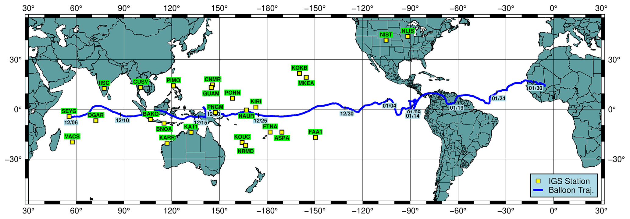
Figure D1Map of balloon trajectory and selected ground stations from the IGS network that are used in determining the regional GPS satellite clock errors.
The Strateole-2 balloon-borne ROC dataset from the 2019 flight is available at the Haase research group web page (https://agsweb.ucsd.edu/strateole2/, last access: 1 May 2020) and also from the Strateole-2 project website managed at the Institut Pierre-Simon Laplace (IPSL), France (https://observations.ipsl.fr/aeris/strateole2/data/C0/ROC/, last access: 1 May 2020). The radiosonde data were downloaded from the University of Wyoming (http://weather.uwyo.edu/upperair/sounding.html, last access: 1 May 2020). The COSMIC-2 provisional data were retrieved from the University Corporation for Atmospheric Research (UCAR) COSMIC Data Analysis and Archive Center (CDDAC) (https://cdaac-www.cosmic.ucar.edu/, last access: 1 May 2020, UCAR COSMIC Program, 2019). The ERA5 reanalysis data were retrieved from the ECMWF Meteorological Archival and Retrieval System (MARS) (https://www.ecmwf.int/en/forecasts/dataset/ecmwf-reanalysis-v5, last access: 1 May 2020, Hersbach et al., 2017). The ground GPS data for selected IGS stations were downloaded from the NASA Crustal Dynamics Data Information System (CDDIS) (https://cddis.nasa.gov/archive/gnss/products, last access: 1 May 2020, Crustal Dynamics Data Information System, 2020). The precise GPS orbit data were downloaded from the Center for Orbit Determination in Europe (CODE) operated at the Astronomical Institute of the University of Bern (http://ftp.aiub.unibe.ch/, last access: 1 May 2020, Dach et al., 2020). All the map products were made using GMT software (https://www.generic-mapping-tools.org/, Wessel et al., 2019).
JSH designed the experiments. JSH and BC developed the instrument and carried out the ROC field deployment. AH oversaw the planning and implementation of the larger Strateole-2 campaign and the collection of the TSEN data. BC processed and analyzed the data with help from all co-authors. MJA contributed analysis of the TSEN data. BC and JSH prepared the manuscript with contributions from all co-authors.
The authors declare that they have no conflict of interest.
Publisher’s note: Copernicus Publications remains neutral with regard to jurisdictional claims in published maps and institutional affiliations.
Development of the ROC version-2 instrument and data collection was supported by National Science Foundation (NSF) award AGS-1642650. The work by M. Joan Alexander and Martina Bramberger was supported by National Science Foundation (NSF) award AGS-1642644. Infrastructure for the international Strateole-2 balloon campaign was provided by NSF, the French National Centre for Space Studies (CNES), and the French National Centre for Scientific Research Dynamic Meteorology Laboratory (LMD). CNES provided the balloons, flight control systems in the gondola Euros, and flight control center. LMD provided the science payload gondola Zephyr, which carried the scientific instruments, including ROC, as well as the science data transmission equipment, and provided the associated mission control center (MCC) for monitoring and control of the instruments and the dataset collection. We thank LMD and LATMOS for engineering support in the field. The balloons were released from the Seychelles International Airport on Mahé, Seychelles, with the local support of the Seychelles Meteorological Authority. We sincerely appreciate their technical and logistical support during the testing and deployment of the ROC receiver. The ROC version-2 receivers were built with the assistance of Dave Jabson of Brainstorm Engineering; John Souders and Sean McPeak of SIO (UCSD), and Steven Liang of UCSD. Stig Syndergaard is acknowledged for providing the original ROSAP ray-tracing model. We acknowledge the support of the National Oceanic and Atmospheric Administration (NOAA) Aircraft Operations Center, in particular, Gabriel Defeo and Jack Parrish, for helping test the ROC receiver on the G-IV aircraft. We also acknowledge technical support from Septentrio Inc., Technologic Systems Inc., UNAVCO, and the United States Antarctic Program (USAP) during the development and testing of the ROC receiver.
This research has been supported by the National Science Foundation (grant no. AGS-1642650).
This paper was edited by Peter Haynes and reviewed by Peter Haynes and one anonymous referee.
Variational Atmospheric Retrieval Scheme (VARS) for GPS Radio Occultation Data, Tech. rep., COSMIC Project Office, University Corporation for Atmospheric Research, 2005. a
Alexander, M. J. and Ortland, D. A.: Equatorial waves in High Resolution Dynamics Limb Sounder (HIRDLS) data, J. Geophys. Res.-Atmos., 115, D24111, https://doi.org/10.1029/2010JD014782, 2010. a, b
Alexander, M. J., Geller, M., McLandress, C., Polavarapu, S., Preusse, P., Sassi, F., Sato, K., Eckermann, S., Ern, M., Hertzog, A., Kawatani, Y., Pulido, M., Shaw, T. A., Sigmond, M., Vincent, R., and Watanabe, S.: Recent developments in gravity-wave effects in climate models and the global distribution of gravity-wave momentum flux from observations and models, Q. J. Roy. Meteor. Soc., 136, 1103–1124, https://doi.org/10.1002/qj.637, 2010. a
Antonita, T. M., Ramkumar, G., Kishore Kumar, K., and Sunil Kumar, S. V.: Quantification of gravity wave forcing in driving the stratospheric Quasi-Biennial Oscillation, Geophys. Res. Lett., 35, L09805, https://doi.org/10.1029/2008GL033960, 2008. a
Baldwin, M. P., Gray, L. J., Dunkerton, T. J., Hamilton, K., Haynes, P. H., Randel, W. J., Holton, J. R., Alexander, M. J., Hirota, I., Horinouchi, T., Jones, D. B. A., Kinnersley, J. S., Marquardt, C., Sato, K., and Takahashi, M.: The Quasi-Biennial Oscillation, Rev. Geophys., 39, 179–229, https://doi.org/10.1029/1999RG000073, 2001. a
Boccara, G., Hertzog, A., Vincent, R. A., and Vial, F.: Estimation of Gravity Wave Momentum Flux and Phase Speeds from Quasi-Lagrangian Stratospheric Balloon Flights, Part I: Theory and Simulations, J. Atmos. Sci, 65, 3042–3055, https://doi.org/10.1175/2008JAS2709.1, 2008. a
Born, M. and Wolf, E.: Principles of optics: electromagnetic theory of propagation, interference and diffraction of light, Cambridge University Press, New York, 7th (expanded) edn., ISBN 0521642221, 1999. a
Bushell, A. C., Anstey, J. A., Butchart, N., Kawatani, Y., Osprey, S. M., Richter, J. H., Serva, F., Braesicke, P., Cagnazzo, C., Chen, C.-C., Chun, H.-Y., Garcia, R. R., Gray, L. J., Hamilton, K., Kerzenmacher, T., Kim, Y.-H., Lott, F., McLandress, C., Naoe, H., Scinocca, J., Smith, A. K., Stockdale, T. N., Versick, S., Watanabe, S., Yoshida, K., and Yukimoto, S.: Evaluation of the Quasi-Biennial Oscillation in global climate models for the SPARC QBO-initiative, Q. J. Roy. Meteor. Soc., 1, 1459–1489, https://doi.org/10.1002/qj.3765, 2020. a
Chen, X. M., Chen, S.-H., Haase, J. S., Murphy, B. J., Wang, K.-N., Garrison, J. L., Chen, S. Y., Huang, C. Y., Adhikari, L., and Xie, F.: The Impact of Airborne Radio Occultation Observations on the Simulation of Hurricane Karl (2010), Mon. Weather Rev., 146, 329–350, https://doi.org/10.1175/MWR-D-17-0001.1, 2018. a
Crustal Dynamics Data Information System (CDDIS DAAC): International GNSS Service, Daily 30-second observation data, NASA EOSDIS CDDIS DAAC [data set], https://doi:10.5067/GNSS/gnss_daily_o_00, last access: 1 May 2020. a
Corcos, M., Hertzog, A., Plougonven, R., and Podglajen, A.: Observation of Gravity Waves at the Tropical Tropopause Using Superpressure Balloons, J. Geophys. Res.-Atmos., 126, e2021JD035165, https://doi.org/10.1029/2021JD035165, 2021. a
Dach, R., Schaer, S., Arnold, D., Kalarus, M. S., Prange, L., Stebler, P., Villiger, A., and Jäggi, A.: CODE final product series for the IGS, Astronomical Institute, University of Bern [data set], https://doi.org/10.7892/boris.75876.4, 2020. a, b
de la Torre, A., Alexander, P., Schmidt, T., Llamedo, P., and Hierro, R.: On the distortions in calculated GW parameters during slanted atmospheric soundings, Atmos. Meas. Tech., 11, 1363–1375, https://doi.org/10.5194/amt-11-1363-2018, 2018. a
Ern, M. and Preusse, P.: Quantification of the contribution of equatorial Kelvin waves to the QBO wind reversal in the stratosphere, Geophys. Res. Lett., 36, L21801, https://doi.org/10.1029/2009GL040493, 2009. a, b, c
Ern, M., Preusse, P., Krebsbach, M., Mlynczak, M. G., and Russell III, J. M.: Equatorial wave analysis from SABER and ECMWF temperatures, Atmos. Chem. Phys., 8, 845–869, https://doi.org/10.5194/acp-8-845-2008, 2008. a
Ern, M., Ploeger, F., Preusse, P., Gille, J. C., Gray, L. J., Kalisch, S., Mlynczak, M. G., Russell, J. M., and Riese, M.: Interaction of gravity waves with the QBO: A satellite perspective, J. Geophys. Res.-Atmos., 119, 2329–2355, https://doi.org/10.1002/2013JD020731, 2014. a
European Centre for Medium-Range Weather Forecasts: ERA5 Reanalysis (0.25 Degree Latitude-Longitude Grid), https://doi.org/10.5065/BH6N-5N20, 2019. a
Fjeldbo, G. and Eshleman, V. R.: The atmosphere of Mars analyzed by integral inversion of the Mariner IV occultation data, Planet. Space Sci., 16, 1035–1059, https://doi.org/10.1016/0032-0633(68)90020-2, 1968. a
Ge, M., Gendt, G., Rothacher, M., Shi, C., and Liu, J.: Resolution of GPS carrier-phase ambiguities in Precise Point Positioning (PPP) with daily observations, J. Geodesy, 82, 389–399, https://doi.org/10.1007/s00190-007-0187-4, 2008. a
Geng, J., Shi, C., Ge, M., Dodson, A. H., Lou, Y., Zhao, Q., and Liu, J.: Improving the estimation of fractional-cycle biases for ambiguity resolution in precise point positioning, J. Geodesy, 86, 579–589, https://doi.org/10.1007/s00190-011-0537-0, 2011. a
Geng, J., Chen, X., Pan, Y., Mao, S., Li, C., Zhou, J., and Zhang, K.: PRIDE PPP-AR: An Open-Source Software for GPS PPP Ambiguity Resolution, GPS Solut., 23, 1–10, https://doi.org/10.1007/s10291-019-0888-1, 2019. a
Haase, J. S., Maldonado-Vargas, J., Rabier, F., Cocquerez, P., Minois, M., Guidard, V., Wyss, P., and Johnson, A. V.: A proof-of-concept balloon-borne Global Positioning System radio occultation profiling instrument for polar studies, Geophys. Res. Lett., 39, l02803, https://doi.org/10.1029/2011GL049982, 2012. a, b
Haase, J. S., Murphy, B. J., Muradyan, P., Nievinski, F. G., Larson, K. M., Garrison, J. L., and Wang, K.-N.: First results from an airborne GPS radio occultation system for atmospheric profiling, Geophys. Res. Lett., 41, 1759–1765, https://doi.org/10.1002/2013GL058681, 2013GL058681, 2014. a, b
Haase, J. S., Alexander, M. J., A. Hertzog, L. K., Deshler, T., Davis, S. M., Plougonven, R., Cocquerez, P., and Venel, S.: Around the world in 84 days, EOS, 99, 32–36, https://doi.org/10.1029/2018EO091907, 2018. a
Haase, J. S., Murphy, M. J., Cao, B., Ralph, F. M., Zheng, M., and Delle Monache, L.: Multi-GNSS Airborne Radio Occultation Observations as a Complement to Dropsondes in Atmospheric River Reconnaissance, J. Geophys. Res.-Atmos., 126, e2021JD034865, https://doi.org/10.1029/2021JD034865, 2021. a, b, c, d
Hajj, G., Kursinski, E., Romans, L., Bertiger, W., and Leroy, S.: A technical description of atmospheric sounding by GPS occultation, J. Atmos. Sol.-Terr. Phy., 64, 451–469, https://doi.org/10.1016/S1364-6826(01)00114-6, 2002. a, b
Healy, S. B., Haase, J., and Lesne, O.: Letter to the Editor Abel transform inversion of radio occultation measurements made with a receiver inside the Earth’s atmosphere, Ann. Geophys., 20, 1253–1256, https://doi.org/10.5194/angeo-20-1253-2002, 2002. a
Hersbach, H., Bell, B., Berrisford, P., Hirahara, S., Horányi, A., Muñoz-Sabater, J., Nicolas, J., Peubey, C., Radu, R., Schepers, D., Simmons, A., Soci, C., Abdalla, S., Abellan, X., Balsamo, G., Bechtold, P., Biavati, G., Bidlot, J., Bonavita, M., De Chiara, G., Dahlgren, P., Dee, D., Diamantakis, M., Dragani, R., Flemming, J., Forbes, R., Fuentes, M., Geer, A., Haimberger, L., Healy, S., Hogan, R.J., Hólm, E., Janisková, M., Keeley, S., Laloyaux, P., Lopez, P., Lupu, C., Radnoti, G., de Rosnay, P., Rozum, I., Vamborg, F., Villaume, S., and Thépaut, J.-N.: Complete ERA5 from 1979: Fifth generation of ECMWF atmospheric reanalyses of the global climate, Copernicus Climate Change Service (C3S) Data Store (CDS) [data set], https://www.ecmwf.int/en/forecasts/dataset/ecmwf-reanalysis-v5 (last access: 1 May 2020), 2017. a
Hersbach, H., Bell, B., Berrisford, P., Hirahara, S., Horányi, A., Muñoz-Sabater, J., Nicolas, J., Peubey, C., Radu, R., Schepers, D., Simmons, A., Soci, C., Abdalla, S., Abellan, X., Balsamo, G., Bechtold, P., Biavati, G., Bidlot, J., Bonavita, M., De Chiara, G., Dahlgren, P., Dee, D., Diamantakis, M., Dragani, R., Flemming, J., Forbes, R., Fuentes, M., Geer, A., Haimberger, L., Healy, S., Hogan, R. J., Hólm, E., Janisková, M., Keeley, S., Laloyaux, P., Lopez, P., Lupu, C., Radnoti, G., de Rosnay, P., Rozum, I., Vamborg, F., Villaume, S., and Thépaut, J.-N.: The ERA5 global reanalysis, Q. J. Roy. Meteor. Soc., 146, 1999–2049, https://doi.org/10.1002/qj.3803, 2020. a
Hertzog, A., Boccara, G., Vincent, R. A., Vial, F., and Cocquerez, P.: Estimation of Gravity Wave Momentum Flux and Phase Speeds from Quasi-Lagrangian Stratospheric Balloon Flights. Part II: Results from the Vorcore Campaign in Antarctica, J. Atmos. Sci., 65, 3056–3070, 2008. a
Ho, S.-P., Anthes, R. A., Ao, C. O., Healy, S., Horanyi, A., Hunt, D., Mannucci, A. J., Pedatella, N., Randel, W. J., Simmons, A., Steiner, A., Xie, F., Yue, X., and Zeng, Z.: The COSMIC/FORMOSAT-3 Radio Occultation Mission after 12 years: Accomplishments, Remaining Challenges, and Potential Impacts of COSMIC-2, B. Am. Meteorol. Soc., 101, 1107–1136 https://doi.org/10.1175/BAMS-D-18-0290.1, 2019. a
Hoeg, P., H., A., K., G., S., S., Belloul, B., Leitinger, R., and Rothleitner, W.: Derivation of atmospheric properties using a radio occultation technique, Sci. Rep., Tech. Rep., Danish Meteorol. Inst., Aalborg, Denmark, 1996. a
Jensen, E. J., Pfister, L., Jordan, D. E., Bui, T. V., Ueyama, R., Singh, H. B., Thornberry, T. D., Rollins, A. W., Gao, R.-S., Fahey, D. W., Rosenlof, K. H., Elkins, J. W., Diskin, G. S., DiGangi, J. P., Lawson, R. P., Woods, S., Atlas, E. L., Rodriguez, M. A. N., Wofsy, S. C., Pittman, J., Bardeen, C. G., Toon, O. B., Kindel, B. C., Newman, P. A., McGill, M. J., Hlavka, D. L., Lait, L. R., Schoeberl, M. R., Bergman, J. W., Selkirk, H. B., Alexander, M. J., Kim, J.-E., Lim, B. H., Stutz, J., and Pfeilsticker, K.: The NASA Airborne Tropical Tropopause Experiment: High-Altitude Aircraft Measurements in the Tropical Western Pacific, B. Am. Meteorol. Soc., 98, 129–143, https://doi.org/10.1175/BAMS-D-14-00263.1, 2017. a
Kawatani, Y. and Hamilton, K.: Weakened stratospheric quasibiennial oscillation driven by increased tropical mean upwelling, Nature, 497, 478–481, https://doi.org/10.1038/nature12140, 2013. a
Kiladis, G. N., Wheeler, M. C., Haertel, P. T., Straub, K. H., and Roundy, P. E.: Convectively coupled equatorial waves, Rev. Geophys., 47, RG2003, https://doi.org/10.1029/2008RG000266, 2009. a, b, c
Kim, J.-E. and Alexander, M. J.: Direct impacts of waves on tropical cold point tropopause temperature, Geophys. Res. Lett., 42, 1584–1592, https://doi.org/10.1002/2014GL062737, 2015. a, b
Kirchengast, G., J., H., and W, P.: The CIRA86aQ_UoG model: An extension of the CIRA-86 monthly tables including humidity tables and a Fortran 95 global moist air climatology model., Tech. Rep. IMG/UoG Techn Rep 8, Eur Space Agency, Paris, France, 1999. a
Kursinski, E. R., Hajj, G. A., Schofield, J. T., Linfield, R. P., and Hardy, K. R.: Observing Earth's atmosphere with radio occultation measurements using the Global Positioning System, J. Geophys. Res.-Atmos., 102, 23429–23465, https://doi.org/10.1029/97JD01569, 1997. a, b, c, d, e
Lemoine, F. G., Kenyon, S. C., Factor, J. K., Trimmer, R., Pavlis, N. K., Chinn, D. S., Cox, C. M., Klosko, S. M., Luthcke, S. B., Torrence, M. H., Wang, Y. M., Williamson, R. G., Pavlis, E. C., Rapp, R. H., and Olson, T. R.: The Development of the Joint NASA GSFC and NIMA Geopotential Model EGM96, Tech. rep., NASA Goddard Space Flight Center, Greenbelt, Maryland, 20771 USA, 1998. a
Lou, Y., Zhang, W., Wang, C., Yao, X., Shi, C., and Liu, J.: The impact of orbital errors on the estimation of satellite clock errors and PPP, Adv. Space Res., 54, 1571–1580, https://doi.org/10.1016/j.asr.2014.06.012, 2014. a
Muradyan, P.: Profiling the atmosphere with the airborne GPS radio occultation technique using open-loop tracking, PhD. thesis, Purdue University, West Lafayette, IN, USA, AAI3544312, 2012. a
Muradyan, P., Haase, J. S., Xie, F., Garrison, J. L., and Voo, J.: GPS/INS navigation precision and its effect on airborne radio occultation retrieval accuracy, GPS Solut., 15, 207–218, https://doi.org/10.1007/s10291-010-0183-7, 2011. a, b
Murphy, B. J.: Profiling the Moisture Environment of Developing Tropical Storms using Airborne Radio Occultation, PhD. thesis, Purdue University, AAI3734541, 2015. a
Murphy, B. J., Haase, J. S., Muradyan, P., Garrison, J. L., and Wang, K.-N.: Airborne GPS radio occultation refractivity profiles observed in tropical storm environments, J. Geophys. Res.-Atmos., 120, 1690–1709, https://doi.org/10.1002/2014JD022931, 2014JD022931, 2015. a, b
Podglajen, A., Hertzog, A., Plougonven, R., and Legras, B.: Lagrangian temperature and vertical velocity fluctuations due to gravity waves in the lower stratosphere, Geophys. Res. Lett., 43, 3543–3553, https://doi.org/10.1002/2016GL068148, 2016. a
Poli, P., Joiner, J., and Kursinski, E. R.: 1DVAR analysis of temperature and humidity using GPS radio occultation refractivity data, J. Geophys. Res.-Atmos., 107, ACL 14–1–ACL 14–20, https://doi.org/10.1029/2001JD000935, 2002. a, b
Rabier, F., Bouchard, A., Brun, E., Doerenbecher, A., Guedj, S., Guidard, V., Karbou, F., Peuch, V.-H., Amraoui, L. E., Puech, D., Genthon, C., Picard, G., Town, M., Hertzog, A., Vial, F., Cocquerez, P., Cohn, S. A., Hock, T., Fox, J., Cole, H., Parsons, D., Powers, J., Romberg, K., VanAndel, J., Deshler, T., Mercer, J., Haase, J. S., Avallone, L., Kalnajs, L., Mechoso, C. R., Tangborn, A., Pellegrini, A., Frenot, Y., Thépaut, J.-N., McNally, A., Balsamo, G., and Steinle, P.: The Concordiasi Project in Antarctica, B. Am. Meteorol. Soc., 91, 69 – 86, https://doi.org/10.1175/2009BAMS2764.1, 2010. a
Ralph, F. M., Cannon, F., Tallapragada, V., Davis, C. A., Doyle, J. D., Pappenberger, F., Subramanian, A., Wilson, A. M., Lavers, D. A., Reynolds, C. A., Haase, J. S., Centurioni, L., Ingleby, B., Rutz, J. J., Cordeira, J. M., Zheng, M., Hecht, C., Kawzenuk, B., and Monache, L. D.: West Coast Forecast Challenges and Development of Atmospheric River Reconnaissance, B. Am. Meteorol. Soc., 101, 1357–1377, https://doi.org/10.1175/BAMS-D-19-0183.1, 2020. a
Randel, W. J., Wu, F., and Rivera Ríos, W.: Thermal variability of the tropical tropopause region derived from GPS/MET observations, J. Geophys. Res.-Atmos., 108, ACL 7–1–ACL 7–12, https://doi.org/10.1029/2002JD002595, 2003. a
Randel, W. J., Wu, F., and Podglajen, A.: Equatorial Waves, Diurnal Tides and Small-Scale Thermal Variability in the Tropical Lower Stratosphere From COSMIC-2 Radio Occultation, J. Geophys. Res.-Atmos., 126, 2020JD033969, https://doi.org/10.1029/2020JD033969, 2021. a
Ravetta, F., Vincent Mariage, Emmanuel Brousse, Eric d´Almeida, Frédéric Ferreira , Jacques Pelon, and Stéphane Victori: BeCOOL: A Balloon-Borne Microlidar System Designed for Cirrus and Convective Overshoot Monitoring, EPJ Web Conf., 237, 07003, https://doi.org/10.1051/epjconf/202023707003, 2020. a
Richter, J. H., Butchart, N., Kawatani, Y., Bushell, A. C., Holt, L., Serva, F., Anstey, J., Simpson, I. R., Osprey, S., Hamilton, K., Braesicke, P., Cagnazzo, C., Chen, C.-C., Garcia, R. R., Gray, L. J., Kerzenmacher, T., Lott, F., McLandress, C., Naoe, H., Scinocca, J., Stockdale, T. N., Versick, S., Watanabe, S., Yoshida, K., and Yukimoto, S.: Response of the Quasi-Biennial Oscillation to a warming climate in global climate models, Q. J. Roy. Meteor. Soc., 1, 1490–1518, https://doi.org/10.1002/qj.3749, 2020. a
Rüeger, J.: Refractive index formulae for electronic distance measurements with radio and millimetre waves, Rep. Unisurv Rep, 109, 758–766, 2002. a
Saastamoinen, J.: Atmospheric Correction for the Troposphere and Stratosphere in Radio Ranging Satellites, American Geophysical Union (AGU), 247–251, https://doi.org/10.1029/GM015p0247, 1972. a
Salby, M. L., Hartmann, D. L., Bailey, P. L., and Gille, J. C.: Evidence for Equatorial Kelvin Modes in Nimbus-7 LIMS, J. Atmos. Sci., 41, 220–235, https://doi.org/10.1175/1520-0469(1984)041<0220:EFEKMI>2.0.CO;2, 1984. a
Sato, K. and Dunkerton, T. J.: Estimates of momentum flux associated with equatorial Kelvin and gravity waves, J. Geophys. Res.-Atmos., 102, 26247–26261, https://doi.org/10.1029/96JD02514, 1997. a, b, c
Scherllin-Pirscher, B., Steiner, A. K., Anthes, R. A., Alexander, M. J., Alexander, S. P., Biondi, R., Birner, T., Kim, J., Randel, W. J., Son, S.-W., Tsuda, T., and Zeng, Z.: Tropical Temperature Variability in the UTLS: New Insights from GPS Radio Occultation Observations, J. Climate, 34, 2813–2838, https://doi.org/10.1175/jcli-d-20-0385.1, 2021. a, b
Schmidt, T., Alexander, P., and de la Torre, A.: Stratospheric gravity wave momentum flux from radio occultations, J. Geophys. Res.-Atmos., 121, 4443–4467, https://doi.org/10.1002/2015JD024135, 2016. a
Schreiner, W., Weiss, J., Anthes, R., Braun, J., Chu, V., Fong, J., Hunt, D., Kuo, Y.-H., Meehan, T., Serafino, W., Sjoberg, J., Sokolovskiy, S., Talaat, E., Wee, T., and Zeng, Z.: COSMIC-2 Radio Occultation Constellation: First Results, Geophys. Res. Lett., 47, e2019GL086841, https://doi.org/10.1029/2019GL086841, 2020. a
Shi, C., Zhao, Q., Geng, J., Lou, Y., Ge, M., and Liu, J.: Recent development of PANDA software in GNSS data processing, in: International Conference on Earth Observation Data Processing and Analysis (ICEODPA), edited by Li, D., Gong, J., and Wu, H., vol. 7285, International Society for Optics and Photonics, SPIE, 558–566, https://doi.org/10.1117/12.816261, 2008. a
Shiotani, M., Gille, J. G., and Roche, A. E.: Kelvin waves in the equatorial lower stratosphere as revealed by cryogenic limb array etalon spectrometer temperature data, J. Geophys. Res.-Atmos., 102, 26131–26140, https://doi.org/10.1029/96JD04012, 1997. a
Simmons, A. J. and Burridge, D. M.: An Energy and Angular-Momentum Conserving Vertical Finite-Difference Scheme and Hybrid Vertical Coordinates, Mon. Weather Rev., 109, 758–766, 1981. a
Srikanth, R. and Ortland, D. A.: Analysis of Kelvin waves in High-Resolution Doppler Imager and Microwave Limb Sounder stratosphere measurements using a constrained least squares method, J. Geophys. Res.-Atmos., 103, 23131–23151, https://doi.org/10.1029/98JD02020, 1998. a
Syndergaard, S.: Modeling the impact of the Earth's oblateness on the retrieval of temperature and pressure profiles from limb sounding, J. Atmos. Sol.-Terr. Phy., 60, 171–180, https://doi.org/10.1016/S1364-6826(97)00056-4, 1998. a, b
Trenberth, K. E., Berry, J. C., and Buja, L. E.: Vertical Interpolation and Truncation of Model-coordinate Data (No. NCAR/TN-396+STR), Tech. rep., University Corporation for Atmospheric Research, https://doi.org/10.5065/D6HX19NH, 1993. a
Tsuda, T., Murayama, Y., Wiryosumarto, H., Harijono, W. B., and Kato, S.: Radiosonde observations of equatorial atmosphere dynamics over Indonesia: 1. Equatorial waves and diurnal tides, J. Geophys. Res.-Atmos., 99, 10491–10505, https://doi.org/10.1029/94JD00355, 1994. a
Tsuda, T., Nishida, M., Rocken, C., and Ware, R. H.: A global morphology of gravity wave activity in the stratosphere revealed by the GPS occultation data (GPS/MET), J. Geophys. Res., 105, 7257–7273, 2000. a
Tsuda, T., Lin, X., Hayashi, H., and Noersomadi: Analysis of vertical wave number spectrum of atmospheric gravity waves in the stratosphere using COSMIC GPS radio occultation data, Atmos. Meas. Tech., 4, 1627–1636, https://doi.org/10.5194/amt-4-1627-2011, 2011. a
UCAR COSMIC Program: COSMIC-2 Data Products, UCAR/NCAR-COSMIC [data set], https://doi.org/10.5065/T353-C093 (last access: 1 May 2020), 2019. a
Vincent, R. A. and Alexander, M. J.: Balloon-Borne Observations of Short Vertical Wavelength Gravity Waves and Interaction With QBO Winds, J. Geophys. Res.-Atmos., 125, e2020JD032779, https://doi.org/10.1029/2020JD032779, 2020. a, b
Vincent, R. A. and Hertzog, A.: The response of superpressure balloons to gravity wave motions, Atmos. Meas. Tech., 7, 1043–1055, https://doi.org/10.5194/amt-7-1043-2014, 2014. a
Vorobév, V. V. and Krasilńikova, T. G.: Estimation of the accuracy of the atmospheric refractive index recovery from Doppler shift measurements at frequencies used in the NAVSTAR system, Phys. Atmos. Ocean, 29, 602–609, 1994. a
Weiss, J.-P., Schreiner, W. S., Braun, J. J., Xia-Serafino, W., and Huang, C.-Y.: COSMIC-2 Mission Summary at Three Years in Orbit, Atmosphere, 13, 1409, https://doi.org/10.3390/atmos13091409, 2022. a
Wessel, P., Luis, J. F., Uieda, L., Scharroo, R., Wobbe, F., Smith, W. H. F., and Tian, D.: The Generic Mapping Tools version 6, Geochem. Geophys. Geosys., 20, 5556–5564, https://doi.org/10.1029/2019GC008515, 2019. a
Wright, C. J., Rivas, M. B., and Gille, J. C.: Intercomparisons of HIRDLS, COSMIC and SABER for the detection of stratospheric gravity waves, Atmos. Meas. Tech., 4, 1581–1591, https://doi.org/10.5194/amt-4-1581-2011, 2011. a
Xie, F., Haase, J. S., and Syndergaard, S.: Profiling the Atmosphere Using the Airborne GPS Radio Occultation Technique: A Sensitivity Study, IEEE T. Geosci. Remote Sens., 46, 3424–3435, https://doi.org/10.1109/TGRS.2008.2004713, 2008. a, b, c
Zeng, Z., Ho, S.-P., Sokolovskiy, S., and Kuo, Y.-H.: Structural evolution of the Madden-Julian Oscillation from COSMIC radio occultation data, J. Geophys. Res.-Atmos., 117, D22108, https://doi.org/10.1029/2012JD017685, 2012. a
Zhang, W., Haase, J. S., Hertzog, A., Lou, Y., and Vincent, R.: Improvement of stratospheric balloon GPS positioning and the impact on gravity wave parameter estimation for the Concordiasi campaign in Antarctica, J. Geophys. Res.-Atmos., 121, 9977–9997, https://doi.org/10.1002/2015JD024596, 2016. a, b
- Abstract
- Introduction
- Method
- Strateole-2 campaign
- Data analysis
- Retrieval results and data quality
- Equatorial waves in the BRO dataset
- Discussion
- Conclusions
- Appendix A: Geometry of balloon-borne RO
- Appendix B: Horizontal resolution
- Appendix C: Water vapor pressure
- Appendix D: IGS ground stations
- Code and data availability
- Author contributions
- Competing interests
- Disclaimer
- Acknowledgements
- Financial support
- Review statement
- References