Sources of concentric gravity waves generated by a moving mesoscale convective system in southern Brazil

The studies on the sources of three concentric gravity waves (CGWs) excited by a moving mesoscale convective system (MCS) on the night of 1–2 October 2019 are investigated. These CGWs were observed using a hydroxyl (OH) all-sky imager, whereas the MCS was observed by the Geostationary Operational Environmental Satellite (GOES). Using 2D spectral analysis, we observed that the three CGWs have horizontal wavelength λ_H between ∼30–55 km, phase speed c_H∼70–90 m s⁻¹, and period τ∼7–12 min. Using backward ray tracing, we found that two of the CGWs were excited from convective cores within the MCS. We also found that the epicenters of the two waves were close to the tropopause positions of the ray-traced paths and nearby convective cores. Regarding the source, we verified that on this night the tropopause was $\sim -$80 ^∘C, which was ∼10 ^∘C colder than the days preceding and after the MCS and also colder than usually observed. Since the tropopause height and temperature are fundamental parameters underlying the analysis of the overshooting extent, we developed our own methodology to establish a reference tropopause that would enable a quantitative estimate of this parameter. Since the MCS (CGWs source) was moving, the overshooting convective cores were tracked in space and time. Using the tracking of the overshooting tops (OTs) in space and time with the aid of reverse ray tracing, we found that two out of the three CGWs were excited by the MCS, whereas the source of the remaining one was not directly associated with the MCS.

1 Introduction

Atmospheric gravity waves (AGWs or simply GWs) play a vital role in the dynamics and thermodynamics of the middle (Fritts and Alexander, 2003) and upper atmosphere (Yiğit et al., 2021). GWs are excited when a disturbance is introduced between stable layers of the atmosphere by either buoyancy (Gossard and Hooke, 1975) or gravity (Nappo, 2013). During the propagation of generated GWs from the lower to the upper atmosphere, the energy and momentum released to excite the GWs are transported by the waves. The energy and momentum are deposited in the middle and upper atmosphere during the dissipation of GWs, thus contributing to turbulence and mixing, thereby influencing the mean circulation and thermal structure of the middle and upper atmosphere (Fritts and Alexander, 2003; Yiğit and Medvedev, 2009).

There are several known sources of mesospheric GWs among which tropospheric convection and severe weather conditions such as thunderstorms are considered the most important and natural sources of GWs in the tropical troposphere. Tropospheric convection has three main GW generation mechanisms, that is, pure thermal forcing, an “obstacle” or “transient mountain” effect, and a “mechanical oscillator” effect. Among these three, the mechanical oscillator effect (overshooting) mechanism is known to be one of the sources of concentric gravity waves (CGWs). Most tropospheric convection–CGW cases in literature have other associated convection-related phenomena, such as hailstorms (Yue et al., 2009; Vadas et al., 2012), lightning (Yue et al., 2014; Nyassor et al., 2021) and transient luminous events (TLEs) (Sentman et al., 2003), which are used as a measure of the severity of the thunderstorm. The relationship between CGWs and deep convection has been established using observations (Yue et al., 2009) and, in some cases, observations complemented by numerical studies (Vadas et al., 2009b, 2012; Nyassor et al., 2021).

Observations of CGWs are made using ground-based instruments, such as all-sky imagers that capture GW activities in the mesosphere in two dimensions (Sentman et al., 2003; Yue et al., 2009, 2013; Vadas et al., 2012; Nyassor et al., 2021, 2022). Satellite imaging data from Atmospheric Infrared Sounder (AIRS) and Visible Infrared Imaging Radiometer Suite (VIIRS) (e.g., Wen et al., 2018; Yue et al., 2014) have also been used to study GW/CGW activities in the stratosphere and mesopause region, respectively. Regarding the observation of tropospheric convective sources of GWs/CGWs, infrared images of cloud top brightness temperature (CTBT) from satellite imagery have been used (Vadas et al., 2009a; Yue et al., 2009; Azeem et al., 2015; Takahashi et al., 2018; Figueiredo et al., 2018; Nyassor et al., 2021, 2022). In most of the reported works on observation of CGWs and deep convection, CTBT images showed overshooting of the tropopause by 1–3 km prior to the observation of the CGWs (Nyassor et al., 2021, 2022, and references therein). Similar works by Vadas et al. (2009a), Vadas et al. (2012), Xu et al. (2015), and Nyassor et al. (2021, 2022) used ray tracing models to relate observed CGWs in hydroxyl (OH) emission altitude (∼87 km) to the overshooting tops in CTBT images captured by the Geostationary Operational Environmental Satellites (GOES).

Some studies also relate satellite observations with outgoing longwave radiation (OLR). These include works by McLandress et al. (2000), Jiang et al. (2004), and Choi et al. (2009) using the Microwave Limb Sounder (MLS). Choi et al. (2009) compared ray-based spectral parameterization of convective gravity wave drag to MLS measurement. They found that the MLS-filtered temperature variances are sensitive to the source-level wave propagation, thus introducing a CGW source model. Preusse et al. (2001) used the CRyogenic Infrared Spectrometers and Telescopes for the Atmosphere (CRISTA) limb sounding during the shuttle missions STS-66 in November 1994 to acquire very high spatial resolution temperature data and mixing ratios of, among other trace gases, tropospheric water vapor. The analyzed structures of the observed GWs exhibit spatial resemblance that is coincident with elevated tropospheric water vapor, suggesting that the observed waves are convectively excited. A typhoon may act as a source of quasi-circular waves of much larger scale, as presented by Kim et al. (2009). Also, recent observational and simulation studies (e.g., Lane et al., 2001; Vadas et al., 2009b; Nyassor et al., 2021) have established a direct relationship between some parameters of observed GWs and some parameters of their respective sources.

Using observational data, Nyassor et al. (2021) established a direct relationship between the period of the observed mesospheric CGWs and the periods of the sources (thunderstorms) using lightning data. They conducted case studies on three CGW events observed in São Martinho da Serra, where the data for this current work were also collected. Using backward ray tracing and the geometric determined center, the CGWs studied were found to be excited by nearby deep convective cores in thunderstorms. A time series CTBT image of the identified source revealed that the entire deep convection was not moving but evolving with time in size. The overshooting tops of the convective cores within these deep convections were estimated and found to overshoot vertically upward into the stratosphere by ∼1–1.5 km. Using the spatial distribution of the lightning densities (obtained by binning the lightning strike in $\mathrm{0.06}{}^{\circ }\times \mathrm{0.06}{}^{\circ }$ grid boxes), the regions with high lightning densities agree with the regions with the coldest cloud top brightness temperature. Using the lightning flash rate, the periodicities in the variations of the updraft/overshooting oscillations were estimated and compared to the CGW periods.

This current study investigates the source positions of CGWs launched from the troposphere by a convective overshooting mechanism in a moving mesoscale convective system (MCS) on 1–2 October 2019 at São Martinho da Serra (29.48^∘ S, 53.87^∘ W). To study the potential propagation path of the CGWs in space and time, leading to the likely source positions and times of CGW excitation, the backward ray tracing model was used. This study is the first to report a moving MCS explicitly (and the overshooting tops, OTs) launching CGWs. So, knowing the source of GWs launched by a system with such characteristics will give more understanding of the dynamics of GWs in the atmosphere. As a result, a novel method has been developed to specifically identify the most likely GW-generating core. The method involves tracking the overshooting convective cores within the system in space and time. Also, the method allows for a further investigation of the convective cores to explore the details of the source (MCS) characteristics in relation to the observed gravity waves.

1.1 The 3D description of the CGW multi-step process and source determination concept

Determining the exact source of CGWs can be challenging when multiple overshooting tops varying in space and time are observed in cloud top infrared (IR) images. The general 3D morphology of the generation, propagation, and observation of CGWs has been described by Nyassor et al. (2021) for a single case of overshooting. For multiple overshooting tops within a moving MCS, the exact OT responsible for the excitation of CGWs needs to be tracked in space and time. In Fig. 1, a 3D diagram shows the multi-step coupling between the lower and upper atmosphere using propagating CGWs generated in the troposphere and observed in the mesosphere.

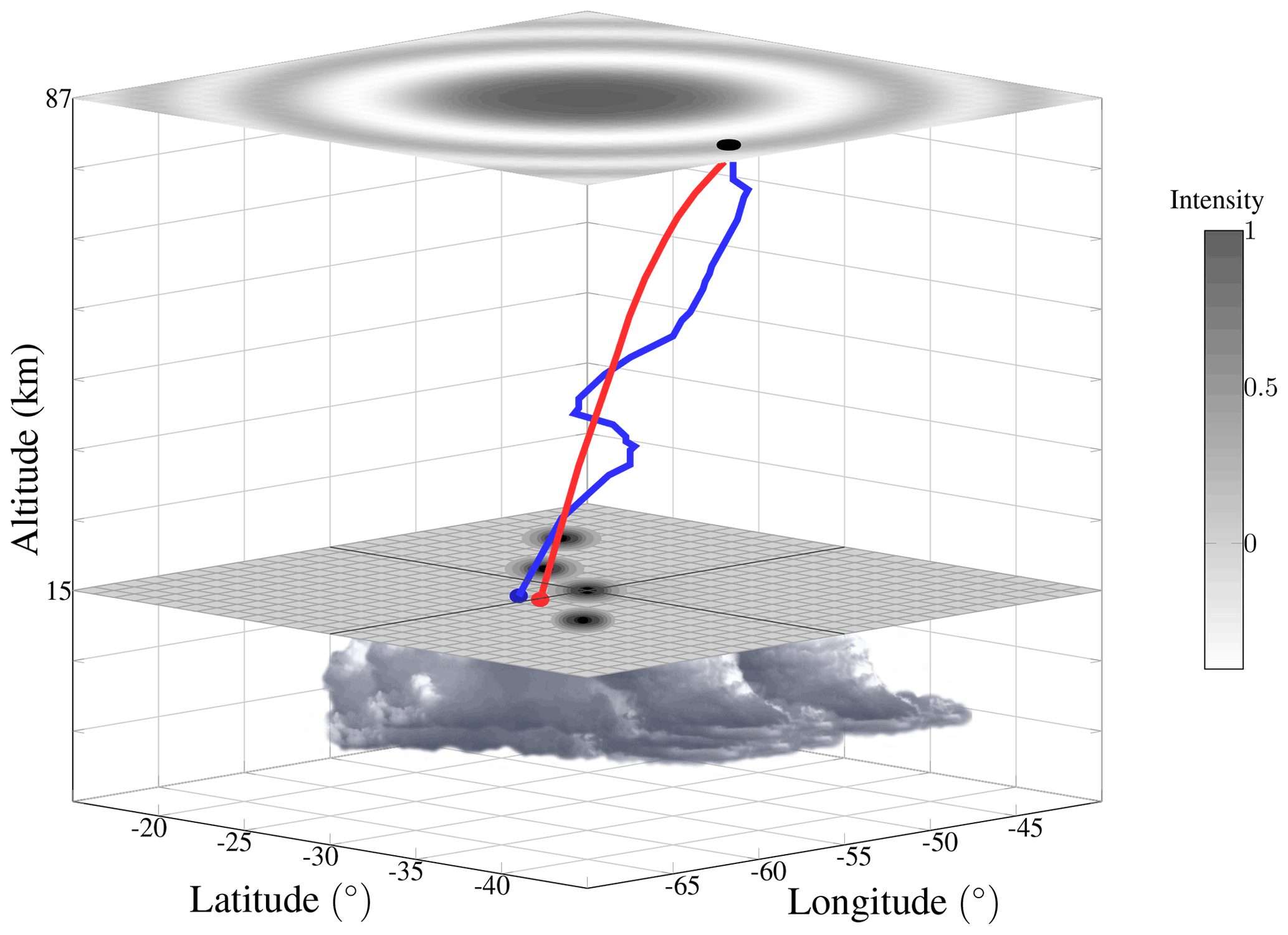
Figure 1 A 3D diagram showing a multi-step process of concentric gravity waves from the generation in the troposphere to the observation in the mesosphere. The red and blue lines show the ray paths of zero and model winds respectively. Circular black patches represent overshooting tops.

In Fig. 1, the observed CGW (circular black (trough) and white (crest) structures) in the OH emission layer at 87 km is reverse-ray-traced to determine the source location in the troposphere. In an atmosphere with background wind, the ray tracing showed that the wave propagated along the solid blue line path, whereas in a windless atmosphere, the wave travels along the solid red line path. The ray paths of the wave stopped in the tropopause, suggesting that this is where the CGW was excited. The tropopause is set at 15 km, with the stable tropopause layer denoted by the stretched gray mesh. At the tropopause, four overshooting tops (circular black region) that originated from the MCS (system of clouds below the tropopause) can be seen close to the stopping position of the ray paths. This work, therefore, aims to determine the most likely OT that excites the observed waves. The general overview of the multi-step coupling between CGW and OT is conceptualized in Fig. 1.

2 Observation and methodology

An OH all-sky airglow imager installed at the Southern Space Observatory (SSO) at São Martinho da Serra (SMS), located at 29.44^∘ S, 53.82^∘ W in the southern part of Brazil, was used for this study. The imager has a single 3 in. OH-NIR (near-infrared) optical filter with a notch at 865.5 nm. Each image has an integration time of 20 s with a sampling rate of 38 s and was cropped from 1024×1024 to 512×512 pixels. The camera is a low-cost front-illuminated charged coupled device (CCD) with 24.5×24.5 mm chip size. The CCD uses a two-stage thermoelectric air cooling system, which can achieve 40 ^∘C below ambient temperature. Further information on this airglow imager can be found in Nyassor et al. (2021).

The observatory also hosts one of the eight observation stations of the TLE and Thunderstorm High Energy Emission Collaborative Network (LEONA). The LEONA TLE stations are installed at different locations in Brazil and Argentina, covering the whole region of Uruguay, Paraguay, Northeastern Argentina, Southern Brazil, and part of Central Brazil. LEONA also has one mobile High Energy Emission Thunderstorm (HEET) station composed of a neutron detector that is normally stationed at INPE headquarters in São José dos Campos but can be moved to be installed anywhere during a field campaign. The TLE station at the SSO, with which the two sprite events reported here were observed, is composed of two Watec low-light video cameras fitted with lenses that yield fields of view of 20–30^∘ and have a previously verified observation range of ∼1100 km into Argentina, Uruguay, and Paraguay (São Sabbas et al., 2010). The cameras are monochromatic with sensitivity in the visible and near-IR wavelengths and are remotely operated in real time during the observations. More information about LEONA can be found in São Sabbas et al. (2019).

The CTBT-captured 10.3 µm infrared (IR) images from channel 13 of the Geostationary Operational Environmental Satellite 16 (GOES-16) provided by the Brazilian Center for Weather Forecast and Climate Studies (CPTEC/INPE) are used to observe and study the MCS activities during the CGW events. The images are taken every 10 min, with each pixel corresponding to approximately 2 km at the Equator. Radiosonde and radio occultation data were used to study the atmospheric vertical temperature profile. Also, associated MCS lightning activities were observed using the Brazilian Lightning Detection Network (BrasilDAT) sensors (Naccarato and Pinto, 2009, 2012; Nyassor et al., 2021).

On 2 October 2019, the SMS OH airglow imager observed curved-like structures emanating from the southwestern part of the observatory between the hours of 00:13 and 04:15 UT. After employing the image preprocessing technique of Garcia et al. (1997) and Wrasse et al. (2007), the unwarped images showed three different concentric structures with different epicenters at separate times. Samples of the unwarped images for each of the observed concentric structures are shown in Fig. 2. The red rectangles highlight the regions where the concentric structures are seen on the OH image. The white triangle indicates the center of the image as well as the location of the observation site.

Figure 2 Sample of unwarped images of each concentric gravity wave (CGW) event observed at São Martinho da Serra on 1–2 October 2019. Panel (a) is Wave no. 01 at 00:27 UT, panel (b) is Wave no. 02 at 00:57 UT, and panel (c) is Wave no. 03 at 04:04 UT. The white triangle shows the center of the image and the SMS observatory, while the red rectangles show the regions of the CGW events.

CGW parameters, the time at which the waves were first identified and their estimated centers in latitude and longitude, are summarized in Table 1. The appearance of the concentric structures in the airglow suggests (1) point-like convective overshooting of the tropopause and (2) weak intervening background wind.

Table 1 Parameters of excited waves during the 1–2 October 2019 CGW events.

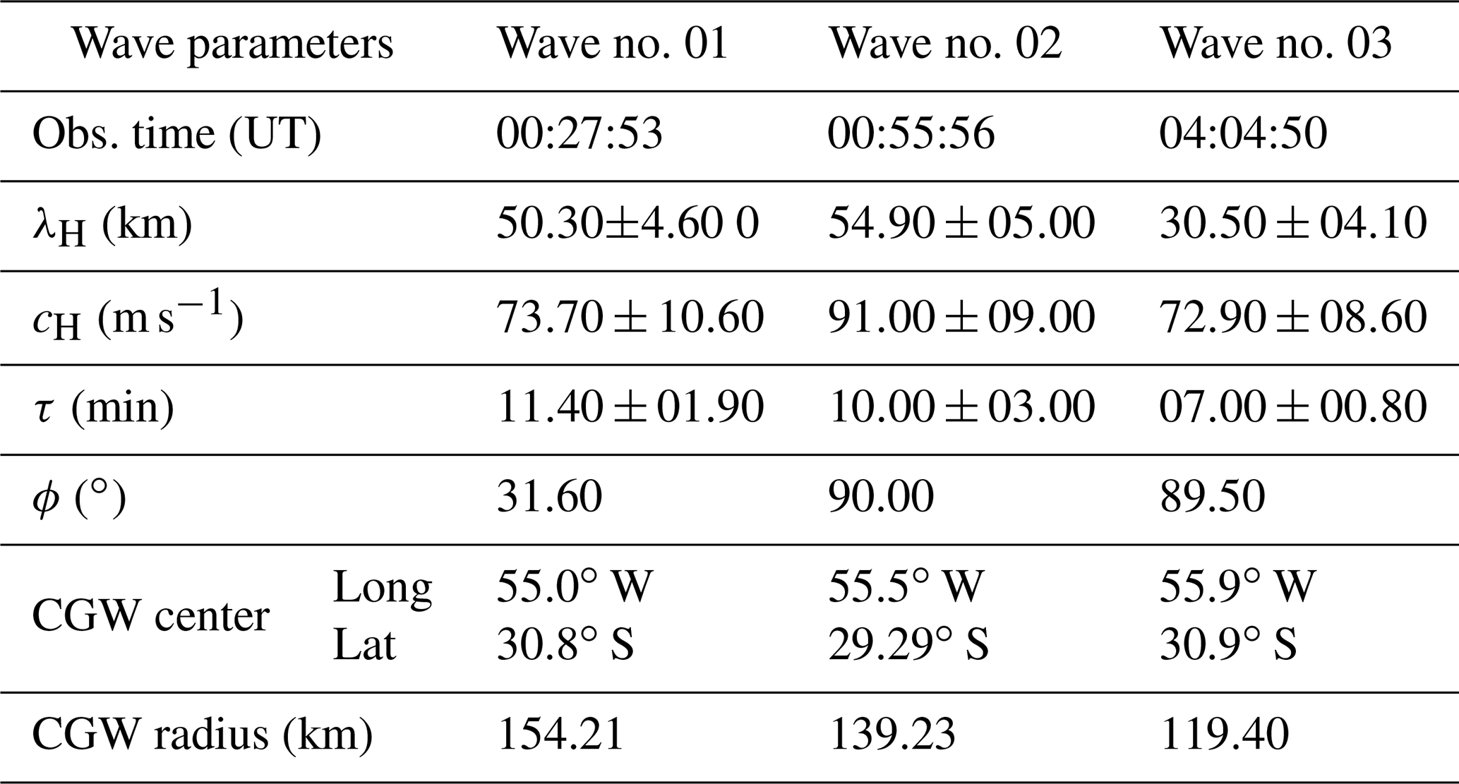
The spatial (horizontal) and temporal parameters of the wave – the wavelength (λ_H), observed period (τ), phase speed (c_H), and propagation direction (ϕ; clockwise from north) of the observed CGWs in the airglow images – were extracted using a two-dimensional spectral analysis technique (Garcia et al., 1997; Wrasse et al., 2007). Due to the annular nature of CGWs, the wave parameters were estimated for three different directions extending from the center of the CGW. For each direction, the wave parameters were estimated assuming a plane wave locally. Then, average values of the parameters of the three directions were computed. The three directions were considered to verify that the observed CGWs emanated from the same point source (Nyassor et al., 2021). The average values of the wave parameters presented in Table 1 are used as input parameters for the ray tracing. However, one propagation direction among the three is chosen to be used in the ray tracing model. To study the propagation of the CGWs and determine their possible source locations, the geometrically determined center and backward ray tracing were used.

2.1 Determination of source locations of the observed waves

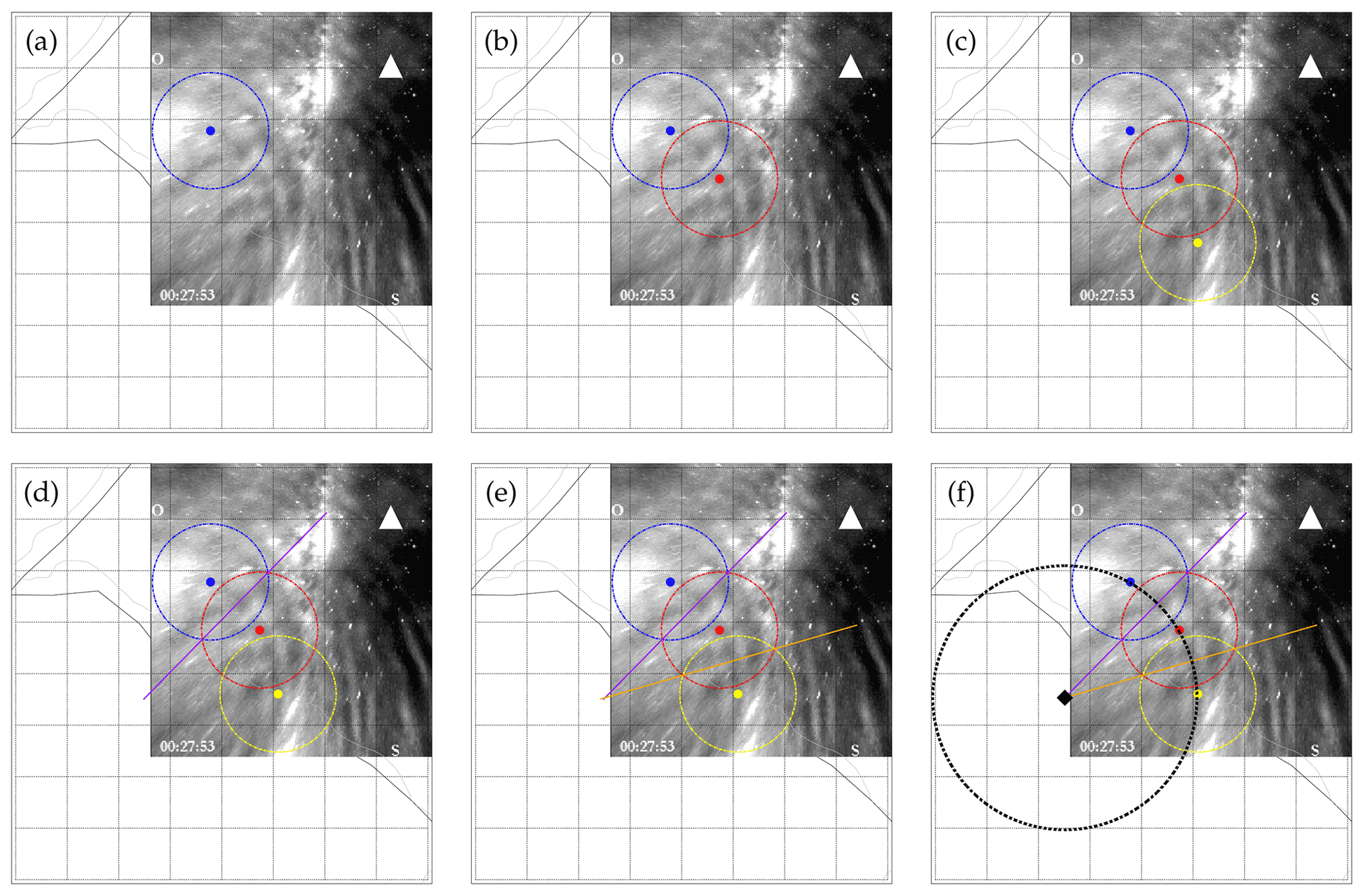
Two methods were used to identify the possible source positions of the CGWs. The first one was the determination of the geometric center of the CGWs, which is a zeroth-order approximation of the source location following the approach of Pedoe (1995) and Nyassor et al. (2021). The description of the methodology used to determine the center of the CGWs is depicted in Fig. 3. It is important to mention that this method can determine the center of arc-like and circular GWs. To determine the geometric center of a CGW, the following steps are used:

1. Three circles of blue, red, and yellow lines of the same radius are constructed in Fig. 3a–c. The respective centers of each circle were drawn over the first visible trough of the first concentric wavefront.

2. Two lines (purple and orange) were constructed through the intersection points of each two adjacent circles.

3. The center of the CGWs is then determined as the intersection point (black diamond in Fig. 3f) of the two intersecting lines shown in Fig. 3e. The radius of the black circle (CGW) is determined by estimating the distance between the center (black diamond) and any of the three centers of the circles drawn in step 1.

Figure 3 Illustration of each step of the methodology used to determine the center of a CGW.

The second method to determine the source location employs a ray tracing model. This model is used to study the propagation of GWs relative to variable background wind in the atmosphere and to determine their possible source location. The propagation of GWs in the presence of background wind enables the investigations of the effect of the wind on a wave. The model employed in this work follows the approach of Vadas (2007), which incorporates kinematic viscosity and thermal diffusivity. To determine the next ray point in space and time, the equations

$$\begin{array}{}\text{(1)}& {\displaystyle \frac{\mathrm{d}{x}_i}{\mathrm{d}t}}=V_i+{\displaystyle \frac{\partial {\mathit{\omega }}_{\mathrm{Ir}}}{\partial k_i}}=V_i+c_{{\mathrm{g}}_i}\end{array}$$

and

$$\begin{array}{}\text{(2)}& {\displaystyle \frac{\mathrm{d}{k}_i}{\mathrm{d}t}}=-k_j{\displaystyle \frac{\partial V_j}{\partial x_i}}-{\displaystyle \frac{\partial {\mathit{\omega }}_{\mathrm{Ir}}}{\partial x_i}}\end{array}$$

were solved numerically using the fourth-order Runge–Kutta routine (Press et al., 2007). The indices i, j=1, 2, 3 indicate the components of vector quantities, position (x), velocity (V), wavenumber (k), and the group velocity c_g. The initial position and time where and when the ray tracing began were the location and time of the first visible concentric crest or trough in the OH emission layer altitude, that is, p_i=(long_i; lat_i; alt_i; t_i). The initial wave vectors (k_x, k_y, m) were obtained from the horizontal component (k_x, k_y) using ${\mathit{\lambda }}_{\mathrm{H}}=\mathrm{2}\mathit{\pi }/k_{\mathrm{H}}=\mathrm{2}\mathit{\pi }/\sqrt{k_x^{\mathrm{2}}+k_y^{\mathrm{2}}}$ and m adapted from the dispersion relation of gravity waves of Vadas (2007):

$$\begin{array}{}\text{(3)}& \begin{array}{rl}{m}^{\mathrm{2}}& ={\displaystyle \frac{k_{\mathrm{H}}^{\mathrm{2}}{N}^{\mathrm{2}}}{{\mathit{\omega }}_{\mathrm{Ir}}^{\mathrm{2}}\left(\mathrm{1}+{\mathit{\delta }}_{+}+{\mathit{\delta }}^{\mathrm{2}}/Pr\right)}}\left[\mathrm{1}+{\displaystyle \frac{{\mathit{\nu }}^{\mathrm{2}}}{\mathrm{4}{\mathit{\omega }}_{\mathrm{Ir}}^{\mathrm{2}}}}{\left({\mathit{k}}^{\mathrm{2}}-{\displaystyle \frac{\mathrm{1}}{\mathrm{4}{H}^{\mathrm{2}}}}\right)}^{\mathrm{2}}\right.\\ & {\left.\cdot {\displaystyle \frac{{\left(\mathrm{1}-P{r}^{-\mathrm{1}}\right)}^{\mathrm{2}}}{{\left(\mathrm{1}+{\mathit{\delta }}_{+}/\mathrm{2}\right)}^{\mathrm{2}}}}\right]}^{-\mathrm{1}}-k_{\mathrm{H}}^{\mathrm{2}}-{\displaystyle \frac{\mathrm{1}}{\mathrm{4}{H}^{\mathrm{2}}}},\end{array}\end{array}$$

where ${\mathit{\delta }}_{+}=\mathit{\delta }(\mathrm{1}+P{r}^{-\mathrm{1}})$, ${\mathit{\nu }}_{+}=\mathit{\nu }(\mathrm{1}+P{r}^{-\mathrm{1}})$, $\mathit{\nu }=\mathit{\mu }/\mathit{\rho }$, and $\mathit{\delta }=\mathit{\nu }m/H{\mathit{\omega }}_{\mathrm{Ir}}$, H is the density scale height, ρ is the density, Pr is the Prandtl number, and ω_Ir is the intrinsic frequency. More details on Eq. (3) can be found in Vadas and Fritts (2006) and Vadas (2007).

The gravity wave parameters, the backgrounds, that is, the wind from the MERRA-2 reanalysis (e.g., Gelaro et al., 2017) and HWM14 (e.g., Drob et al., 2015), temperature from MERRA-2, and NRLMSISE-00 (e.g., Picone et al., 2002) models were used as the input parameters. Due to the altitude limitation of the MERRA-2 wind and temperature, MERRA-2 wind and temperature profiles were concatenated with HWM14 and NRLMSISE-00 profiles, respectively.

The concatenation of the profiles was done to attain the altitude range from 0–100 km since MERRA-2 wind and temperature extends up to 75 km. An altitude range of 65–75 km was set for the MERRA-2 and HWM14 wind to minimize any discontinuities in the profiles. The difference between the two winds at each kilometer within the set range was computed. Then, the altitude with the smallest difference is chosen as the concatenation altitude in order to reduce any potential bias that might be locally induced. Finally, the concatenated profile was smoothed every three points. A similar procedure is also used to concatenate the MERRA-2 and NRLMSISE-00 temperature profiles. Since MERRA-2 has a temporal resolution of 3 h, interpolation was performed for each time step (Nyassor et al., 2021). To perform the iteration for the next step, stopping conditions were defined:

1. Since a GW propagates at the group velocity, this ray tracing is set to propagate slower than the speed of sound (C_s), thus c_g≤0.9C_s, where the factor 0.9 is arbitrarily chosen. Here, $c_{\mathrm{g}}=\sqrt{c_{{\mathrm{g}}_x}^{\mathrm{2}}+c_{{\mathrm{g}}_y}^{\mathrm{2}}+c_{{\mathrm{g}}_z}^{\mathrm{2}}}$ is the group velocity in the wave propagation direction. This condition is set to remove the spectrum of acoustic waves.

2. When a GW encounters a region in the atmosphere where the horizontal phase velocity equals the horizontal wind speed, the GW approaches a critical or absorption level. Physically, the vertical propagation of the wave becomes very slow, thereby causing the wave not to propagate vertically because m→∞. In this condition, the intrinsic frequency of the wave approaches zero in this region, causing the wave to be rapidly absorbed by the atmosphere. Therefore, for the ray tracing to calculate the wave trajectory, it is necessary for the intrinsic frequency of GW to be greater than zero (ω_Ir>0).

3. As GWs propagate higher into the thermosphere, molecular viscosity and thermal diffusivity become an important dissipative process, owing to the decrease in density with altitude. This causes an increase in the momentum flux of GWs in the lower thermosphere until it reaches a maximum value and then decreases rapidly with increasing altitude. This, therefore, implies as GWs attain their maximum momentum flux, they tend to dissipate. Hence, it is necessary for the momentum flux along a GW ray path to satisfy $R_{\mathrm{m}}>{\mathrm{10}}^{-\mathrm{15}}{R}_{\mathrm{0}}$. R_m is the momentum flux at each altitude, and R₀ is the momentum flux at the reference altitude. The factor 10⁻¹⁵ was arbitrarily chosen.

4. The vertical wavelength needs to be smaller than the viscosity scale to ensure that the viscosity will not change too much in time and altitude, that is, $\left[\left|{\mathit{\lambda }}_z\right|<\frac{\mathrm{2}\mathit{\pi }}{\frac{\mathrm{d}\mathit{\nu }/\mathrm{d}z}{\mathit{\nu }}}\right]$. Here, $\mathit{\nu }=\frac{\mathit{\mu }}{\mathit{\rho }}$ is the kinematic viscosity, with μ being molecular viscosity and ρ the density (Vadas, 2007). This condition is necessary because GWs with these characteristics must satisfy the imposed simplifications (slowly varying parameters) to obtain the dispersion relation.

Note that items 3 and 4 are essential when forward ray tracing the waves into the thermosphere.

2.2 Determination of tropopause temperature, altitude, and overshooting tops

Usually, the tropopause is determined using either the lapse rate (Xian and Homeyer, 2019) or cold-point (Kim and Son, 2012) criteria. In this work, both criteria were used to determine the tropopause. It was observed that during the night of the CGW events, the tropopause was colder than usually reported in literature. So, to investigate this colder tropopause temperature, the impact of the MCS on the tropopause from the days before to the days after the night of the CGW events was studied. Some studies (e.g., Sherwood et al., 2003; Kim et al., 2018) suggest that extreme active deep convection appears to cool the layer near the cloud top, thereby causing colder tropopause. On this basis, the variation in the tropopause height and temperature from radiosonde and radio occultation temperature soundings near/around the observation site and the MCS was used to study and verify the effect of the MCS on the tropopause. The radio occultation temperature profiles obtained from 1 to 3 October 2019 were used to verify the behavior of the radiosonde tropopause height and temperature variation are shown in Fig. A1.

To estimate the vertical extension of the overshooting tops, it is important to first properly determine the tropopause temperature and altitude. So, the colder the tropopause, the more energetic the convection needs to be to produce overshooting into the stratosphere. This means that the updraft velocity of the column of rising warm air within the convective system or cloud must be high enough to overshoot significantly. The observation of these three CGWs indicates convective overshooting of the tropopause by at least ∼1–3 km, the criteria for convection to generate GWs, which is considered to be the main mechanism to generate CGWs (Yue et al., 2009; Vadas et al., 2009b, 2012; Nyassor et al., 2021). Two distinct estimation methods of the overshooting tops were used in this work, and their results were compared: (i) the adapted approach of Griffin et al. (2016) used by Nyassor et al. (2021) and (ii) a simplified version of the method of São Sabbas et al. (2009).

The first approach is an approximation in which the tropopause temperature and altitude are obtained from the radiosonde temperature profile. For this approach, the tropopause is the first temperature inversion point. This inversion point was estimated following the definition of the World Meteorological Organization standard (Xian and Homeyer, 2019). Adapting Eq. (4) from Griffin et al. (2016), the overshooting top height (OT_Height) is estimated using the brightness temperature (BT) and the lapse rate (LR) of the overshooting top (OT), the tropopause height, and the temperature.

$$\begin{array}{}\text{(4)}& {\mathrm{OT}}_{\mathrm{Height}}=H_{\mathrm{Trop}}+{\displaystyle \frac{{\mathrm{OT}}_{\mathrm{BT}}-T_{\mathrm{Trop}}}{{\mathrm{OT}}_{\mathrm{LR}}}}\end{array}$$

Here, H_Trop is the tropopause height, OT_BT is the brightness temperature of the OT, T_Trop is the tropopause temperature, and OT_LR is the OT lapse rate.

The cloud top brightness temperature was obtained from the Advanced Baseline Imager (ABI), an imaging radiometer of GOES-R satellite. The ABI has 16 different spectral bands, including 2 visible channels, 4 near-infrared channels, and 10 infrared channels, with a spatial resolution of 0.5–2 km. The CTBT is one of the products derived from the 11, 12, and 13.3 µm infrared observations. The OT lapse rate was estimated using the radiosonde profile and the CTBT. The average OT lapse rate for the days considered in determining the tropopause temperature and altitude was averaged and was found to be −7.35 K km⁻¹.

In the second method to identify the convective cores of a given convective region, we calculated the average temperature ($\stackrel{\mathrm{‾}}{T}$) of the coldest cloud tops and their surroundings (São Sabbas et al., 2009, 2010). To calculate the $\stackrel{\mathrm{‾}}{T}$, we added the temperature of all pixels whose values were lower than a threshold. This threshold is defined as $T\le -\mathrm{70}$ ^∘C. Next, the sum of the temperature lower than the threshold was divided by the total number of pixels. We then calculated the difference between the temperature of the pixel and the average, that is, $\mathrm{\Delta }T=T_{\mathrm{pixel}}-\stackrel{\mathrm{‾}}{T}$. The averaging was performed within a spatial grid of 10×10 km and a temporal range of 10 min. The pixels with the lowest ΔT were selected as the “center” of the convective cores (T_core), and their area was estimated by adding the area of surrounding pixels until $\mathrm{\Delta }T=T_{\mathrm{core}}/\mathrm{2}$. In most cases, the temperature gradient around the convective core center was rather sharp, and the number of pixels with $\mathrm{\Delta }T\le T_{\mathrm{core}}/\mathrm{2}$ was small; thus all of them were included. For the few convective cores that extended to larger areas and/or merged with other convective cores, only a few pixels outward in each direction from the coldest spot were included. The height of the overshooting is estimated by finding the difference between the altitudes of the convective core and the tropopause (Adler and Fenn, 1979; Heymsfield and Blackmer, 1988).

3 Results and discussions

3.1 Ray tracing results of the CGWs

The ray tracing results of the three CGWs are presented in Fig. 4. In Fig. 4a(i)–c(i), the individual path of the CGW trajectory and the MCS at the time the ray path reached the tropopause are presented. The wave crest, tropopause height, observation site, CGW center (of the circle), and the stopping positions of each ray path are represented by the cross, star, triangle, diamond, blue-filled circles, and red-filled circles, respectively. Panel (ii) shows the zoomed-in region depicted by the red square in Fig. 4a without the CTBT and is also used to show the trajectory of the OTs in space around the determined center and the tropopause position of the ray paths. The squares and circles indicate the positions of the convective cores (Cs). The OTs (or Cs) are depicted by the red and orange squares with black outlines and white and red circles with black outlines. The color bar in the upper left corner shows the temperature scale of the cloud top temperature. The time–altitude profiles of the ray paths are shown in panel (iii). In all panels, the blue lines denote the ray path of the wave trajectory using the model wind (i.e., MERRA-2 and HWM14), whereas the red lines represent the ray paths of wave trajectory where zero wind was considered.

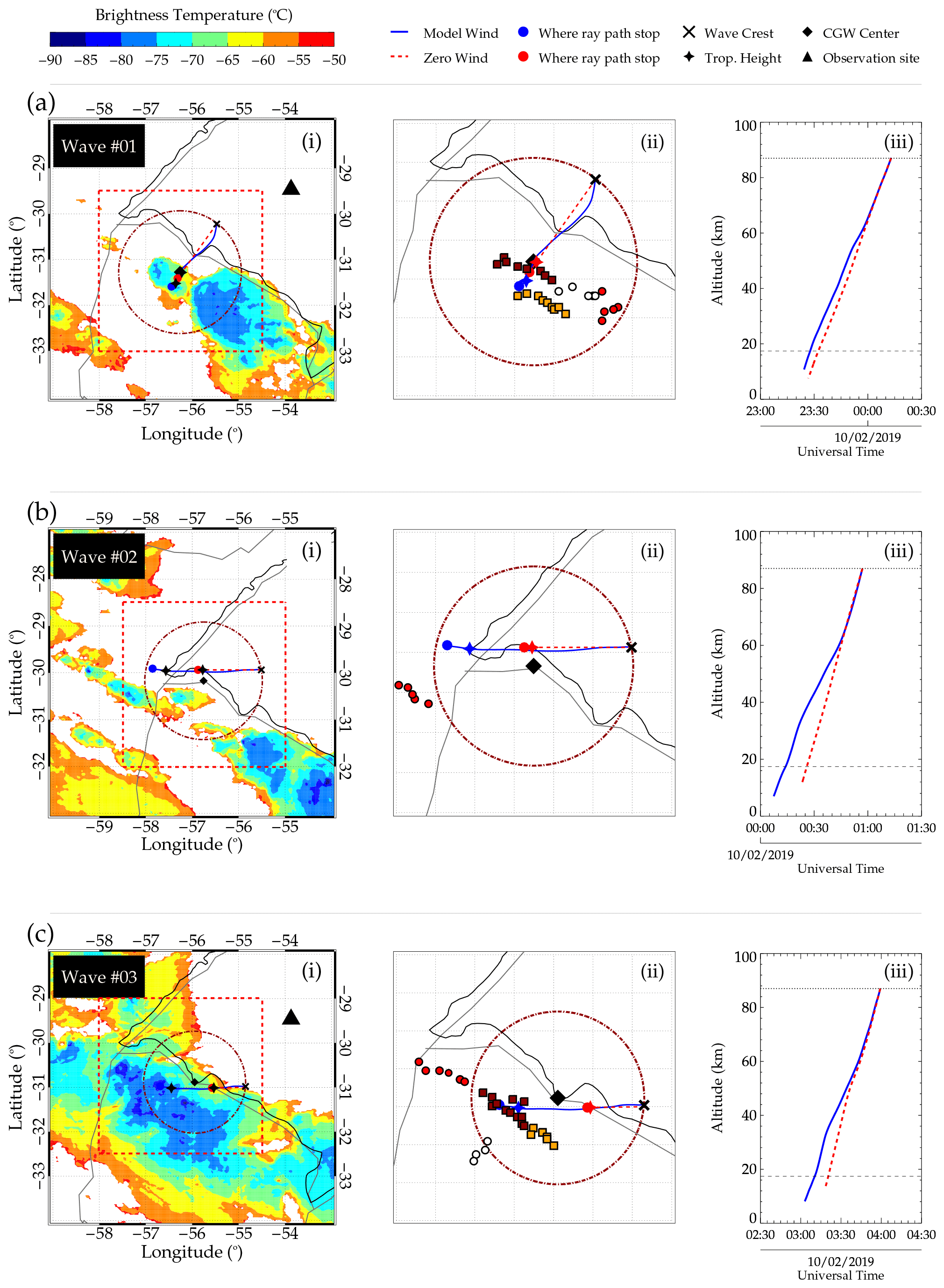
Figure 4 Ray tracing results of concentric gravity wave (CGW) events one (no. 01), two (no. 02), and three (no. 03) on 1–2 October 2019.

The IR cloud top brightness temperature maps shown reflect the status of the MCS closest to the time when the CGW ray path reached the tropopause, which is considered to be the excitation altitude. The coldest CTBT regions have been used to identify convective overshooting tops (Bedka et al., 2010; Jurković et al., 2015) and the possible source of CGWs (Nyassor et al., 2021, and references therein). The OH airglow layer emission at ∼87 km of altitude is the ray tracing starting point, which is denoted by the dotted black line in Fig. 4a(iii)–c(iii). In the same panels, the altitudes of the tropopause obtained from the radiosonde measurement are the dashed black line. Similar cloud top brightness temperature plots with extended longitude and latitude ranges of Fig. 4a(i)–c(i) have been attached in Fig. B1 to show a larger view of the MCS around the CGWs. In Fig. B1, panels (a)–(c) represent Fig. 4a(i)–c(i) respectively.

3.2 Effect of background wind on the CGW propagation

A blocking diagram described by Medeiros et al. (2003), Giongo et al. (2020), and Nyassor et al. (2021) adapted from Taylor et al. (1993) was used to study the state of the background wind relative to the wave propagation. The blocking diagram considers the observed phase speed (c_H) for every known azimuth of the zonal (V_x) and meridional (V_y) wind components, which are given mathematically as

$$\begin{array}{}\text{(5)}& c_{\mathrm{H}}=V_x\cos \mathit{\varphi }+V_y\sin \mathit{\varphi },\end{array}$$

where ϕ is the direction of the wind ($V_{\mathrm{H}}=V_x\cos \mathit{\varphi }+V_y\sin \mathit{\varphi }$) along the wave's propagation direction. Equation (5) is satisfied when V_H approaches c_H and the intrinsic frequency ω_Ir approaches zero at the critical layer. This theory demonstrates the dependency of the intrinsic frequency of atmospheric waves on the background wind. Thus, the blocking diagram is used to visualize the regions where background winds induce a zero vanishing intrinsic frequency of the GWs. The 2D blocking diagram and the 3D projection are presented in Fig. 5. The regions where wave propagation is not allowed (forbidden region) due to the characteristics of the wind in the troposphere correspond to the wind from 0–17 km (red rings). Between the tropopause and mesopause (blue rings), the wind between 18 and 87 km is presented, whereas above 87 to 100 km, the wind is shown by the green rings. Figure 5 was obtained using the average winds between 21:00 UT on 1 October 2019 and 05:00 UT on 2 October 2019.

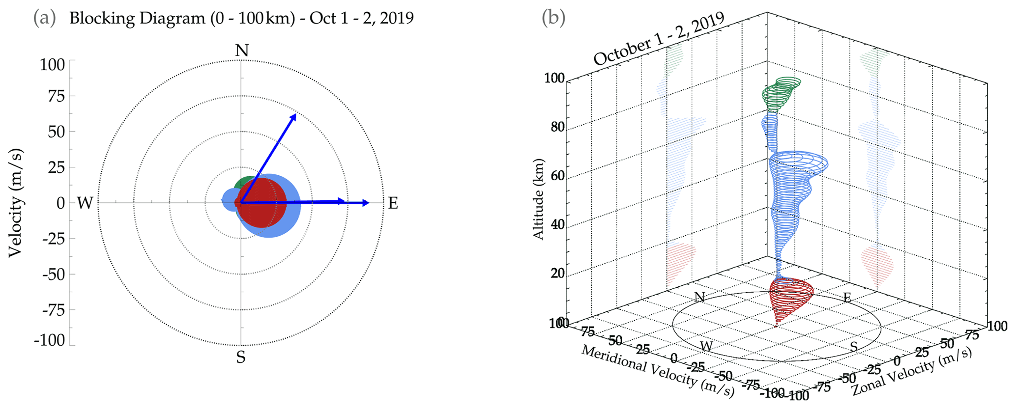
Figure 5 (a) The 2D blocking diagram and (b) the 3D blocking diagram. The wind characteristics from 0–17 km are represented by red rings, from 18–87 km by light-blue rings, and above 87 km by green rings.

From Fig. 5a, weak winds were observed below the mesopause. Even though variations in the magnitude of the winds were observed with altitude (see 3D projection in Fig. 5b), the 2D projection showed that the wind between the mesopause and the ground did not exceed 45 m s⁻¹. Note that the minimum phase speed among the three CGWs is ∼73 m s⁻¹, which is higher than the maximum wind in the eastward direction. The colors used in the differentiation of the winds at each respective altitude range are the same in both panels of Fig. 5. The 2D projection (i.e. Fig. 5a) clearly shows that the winds in the troposphere, stratosphere, and mesosphere were mainly within the northeastern to southeastern direction. The blue arrows in the 2D projection (see Fig. 5a) represent the magnitude and direction of the CGWs.

The filtering effects of the wind on the CGWs are investigated using 2D and 3D blocking diagrams. In the 2D blocking diagram, the magnitude and direction of the horizontal phase speeds of the CGWs are the blue arrows extending from the origin. The blocking regions where wave propagation is prohibited showed quite a directional anisotropy, mainly between the north and east directions. Between the tropopause and mesopause, the winds were mostly between 31–109^∘ with a magnitude < 45 m s⁻¹. This explains the propagation of the CGWs to the OH emission layer altitude with little or no filtering and without distortion of the concentric shapes. As depicted by the ray tracing results (Fig. 4), the background winds were relatively weak during the three CGW events, and hence the small variation in the ray path of the model's wind compared to that of the zero winds, especially for Wave no. 01 and no. 03. The waves observed here have phase speeds sufficiently larger than the background wind and do not introduce major distortions in the wavefronts. Hence, they can still be recognized as concentric wave structures.

3.3 Convective sources

Point-like convective overshooting of the tropopause by 1–3 km into the stratosphere can generate atmospheric GWs with concentric wavefronts (e.g., Lane et al., 2003; Vadas et al., 2009a; Yue et al., 2009; Nyassor et al., 2021). As mentioned earlier, the CTBT from the GOES-16 IR imagery was used to identify the overshooting convective tops, which are possible sources of the observed CGWs. Numerous works (e.g., Taylor and Hapgood, 1988; Sentman et al., 2003; Vadas et al., 2009b; Yue et al., 2009; Nyassor et al., 2021, 2022) related mesospheric OH GWs with concentric wavefronts to convective activity of thunderstorms, particularly with overshooting convective cores of these highly active cloud systems. Using the GOES infrared images, Bedka et al. (2010) used CTBT to detect overshooting tops. Yue et al. (2009) simultaneously identified regions of convective overshooting using reflectivity data from the Next Generation Weather Radar (NEXRAD) and concluded that two convective plumes were the sources of the two interfering CGWs studied in their work. They also noticed that the thunderstorm was already very active with strong convective activity 3–4 h before the CGW observations. Due to this, a detailed investigation is conducted to determine the closest convective core that excites these CGWs.

On 1 October 2019, around 18:40 UT, a warm cloud band started to develop convective regions around 32.0^∘ S, 55.0^∘ W, which grew into a large mesoscale convective system extending from the northwestern to the southeastern part of São Martinho da Serra, Brazil, and into the northern part of Uruguay, seen in the GOES-16 IR images. Just 1 h later, at 19:40 UT, their cloud tops reached about −65 ^∘C, showing an extremely fast vertical growth, indicative of strong updrafts already in the early stages of this thunderstorm development. In half an hour, that is, at 20:10 UT, the cloud tops reached about −70 ^∘C, a characteristic of intense convection; the system became organized into a multicell MCS. By 22:40 UT, we could identify the convective cloud cover of the system over Uruguay, which lasted for more than 24 h. The CTBT map at 22:40 UT is presented in Fig. 6. An animation of the evolution of the MCS between 18:00 UT on 1 October 2019 and 05:50 UT on 2 October 2019 is provided in the video supplement.

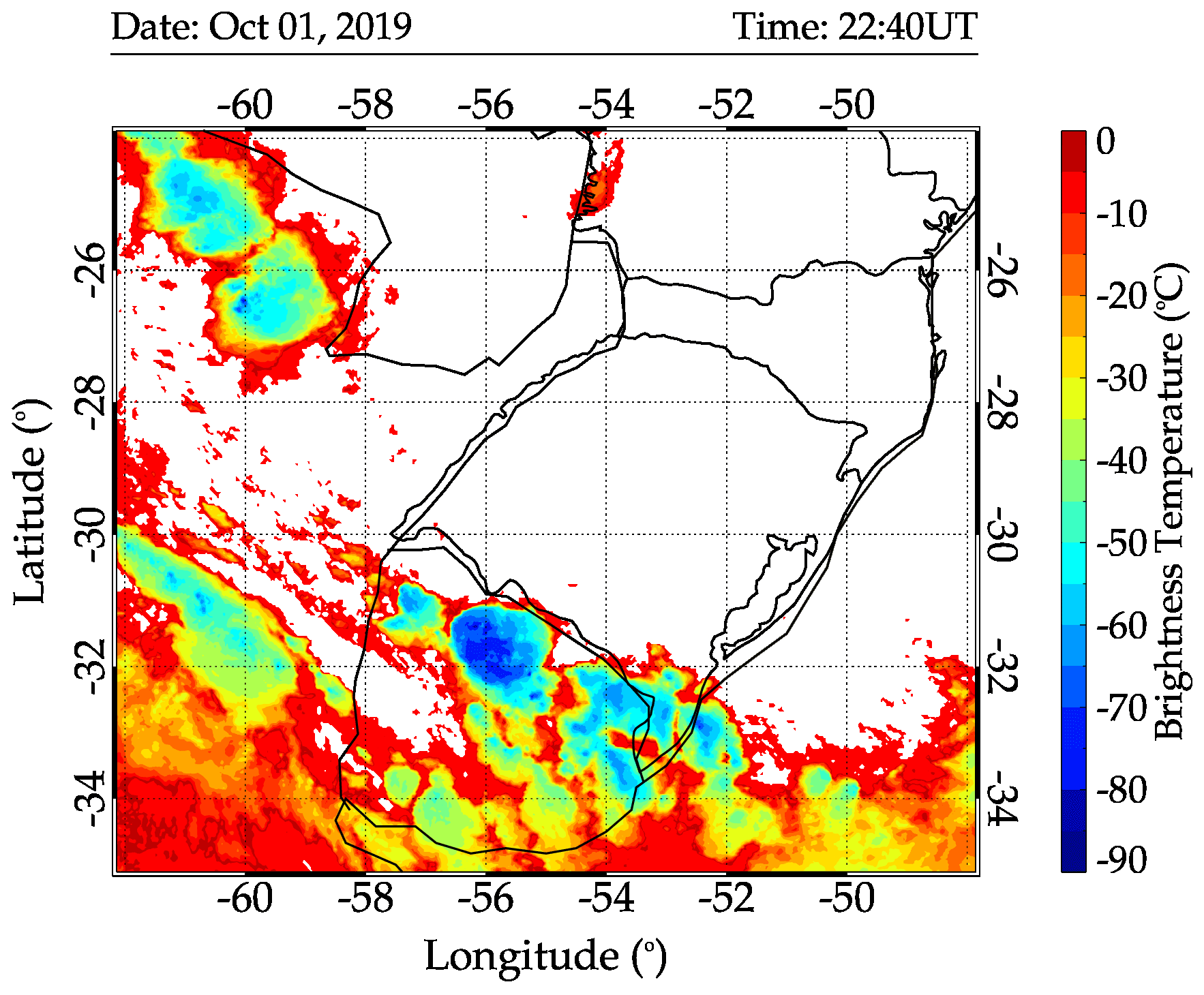
Figure 6 GOES-16 IR image taken at 22:40 UT showing the CGW-generating MCS over Uruguay.

To obtain the tropopause altitude and temperature, the prerequisite parameters to estimate the OT altitude, radiosonde measurements taken at Santa Maria (29.69^∘ S, 53.81^∘ W) from 29 September to 10 October 2019 were used. The tropopause altitudes and temperatures for the 00:00 and 12:00 UT soundings for each day were considered in this analysis. The results of the variations in the tropopause altitudes and temperatures are shown in Fig. 7. The radiosonde measurement at Santa Maria on the night of the CGW events recorded a convective available potential energy (CAPE) (Holton and Hakim, 2012) value of ∼1500 J kg⁻¹ (i.e., a maximum updraft velocity, $w\sim \sqrt{\mathrm{2}\cdot \mathrm{CAPE}}$ of ∼54.45 m s⁻¹). During this event, hail events were reported by Globo News (2019). According to the report, the hail event began in the late hours on 1 October 2019 and continued into the early hours of 2 October 2019, which signifies strong convective activity.

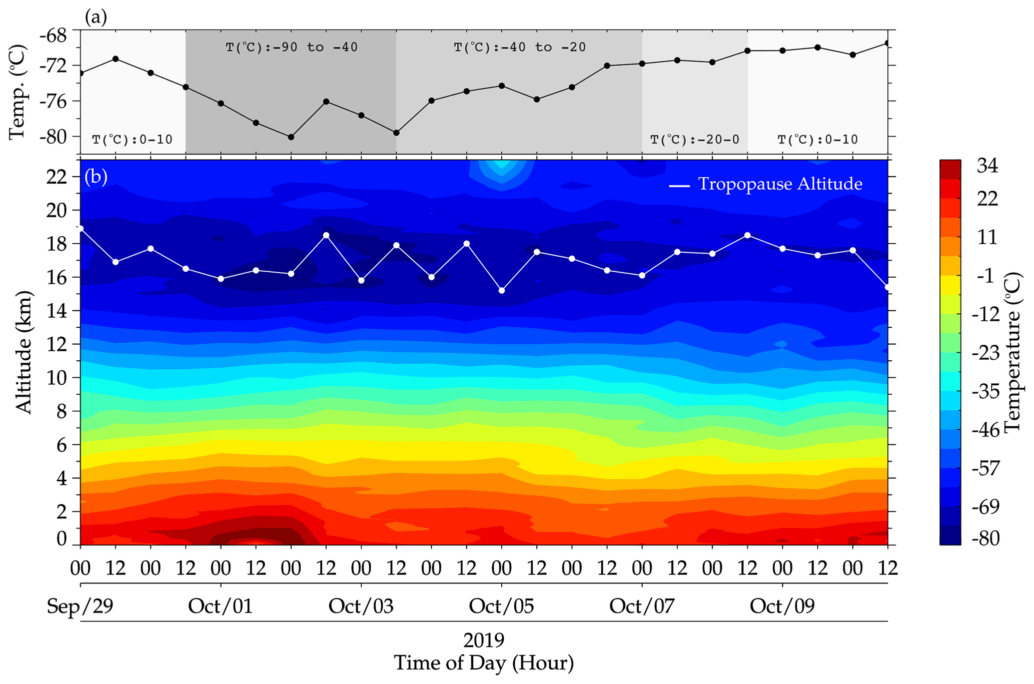
Figure 7 Tropopause temperatures and altitude variations at Santa Maria, RS, Brazil, from 29 September to 10 October 2019, obtained from radiosonde sounding measurements at 00:00 and 12:00 UT. In panel (a), the variation of the tropopause temperature (black line) through the days is presented. The grayscale regions with the label “T(^∘ C)” represent the temperature range of the cloud top. The contour plot in panel (b) shows the temperature profile from 0–23 km through the days considered. The white line shows the variation of the tropopause altitude with their respective temperatures shown in (a).

In Fig. 7a, the variations in the tropopause temperature through the days considered are presented. The grayscale background regions with the label “T (^∘ C)” indicate the cloud top brightness temperature ranges for each day. It was observed in previous studies that the presence of deep convection with colder cloud top brightness temperatures further decreases the tropopause temperature (Kim et al., 2018). In our data this also happens between 12:00 UT on 30 September 2019 and 12:00 UT on 3 October 2019, when the cloud top temperature ranges between $-{\mathrm{40}}^{\circ }$C and $-{\mathrm{90}}^{\circ }$C. As the deep convection dissipates and its cloud top becomes hotter, the tropopause also becomes hotter, as shown in the profiles from 12:00 UT on 3 to 10 October 2019. In Fig. 7b, the general behavior of the temperature from 0–23 km is presented, with the variation in the tropopause altitude over-plotted by the solid white line with dots. The tropopause temperature, at the wave excitation time, has been influenced by the presence of the active deep convection. Therefore, the average of the tropopause temperature ($\sim -\mathrm{74}$ ^∘C) and altitude (∼17 km) of the selected days with and without deep convection was used in the determination of the overshooting extent.

3.4 Tracking OT in space and time

This section discusses the positions and the corresponding times of the OTs. The general result of the temporal variation of the heights of OTs is presented. Afterwards, the spatial variation of the OTs per longitude and latitude at each 10 min of the CTBT maps was examined. Also, the comparison between each respective OT in space and time relative to the ray-traced source location is discussed.

3.4.1 Temporal variation of overshooting tops height

Using the two approaches of overshooting top estimation following the techniques of Griffin et al. (2016) and São Sabbas et al. (2009) highlighted in Sect. 2.2, the extension by which the tropopause was overshot into the stratosphere was estimated. The result of the overshooting top variation using the method of Griffin et al. (2016) is shown in Fig. 8 for each wave. For Wave no. 1, the dark-red and orange squares with black outlines, and white and red circles with black outlines represent the convective cores (Cs) no. 1 to no. 4 on 1 October 2019 from 21:00 UT to 00:00 UT on 2 October. The red circle with a black outline represents C no. 05 overshooting between 00:30–01:30 UT for Wave no. 02. For Wave no. 03 between 02:00–04:10 UT, the convective cores are represented by Cs no. 06, no. 07, no. 08, and no. 09.

Figure 8 Tracking of overshooting tops in time. Panels (a)–(d) show the temporal variation of the overshooting of convective cores (Cs): no. 01, no. 02, no. 03, and no. 04 for Wave no. 01, C no. 05 for Wave no. 02, and Cs no. 06, no. 07, no. 08, and no. 09 for Wave no. 3. The grayscale regions demarcate the regions for each wave event. The dashed lines show the mean overshooting height of each system, whereas the dotted lines show the mean tropopause height between 29 September and 10 October 2019.

3.4.2 Tracking Wave no. 01 in space and time

The ray tracing result of Wave no. 01 shows that the time when the ray paths of both zero and model winds reached the tropopause was 23:27 and 23:32 UT, respectively. Considering only the model wind tropopause time, only Cs no. 03 and no. 04 were active, indicating this could be the launching time of the wave. The OT height corresponding to this time is depicted by the respective large open squares and circles. From Fig. 8, we observed that at the time of launch of Wave no. 01, indicated by the ray tracing, the OT heights for Cs no. 03 and no. 04 are at a minimum. This indicates that Wave no. 01 cannot be launched at this time. For C no. 03 (white circle with black outline), a higher OT height (>1 km) occurred between 22:40 and 23:10 UT and also at 23:40 UT. In the case of C no. 04, OT heights > 1 km were observed at 23:50 and 00:00 UT. This implies that Cs no. 03 and no. 04 can only launch Wave no. 01 between 22:40 and 23:10 UT and 23:40 and 00:00 UT.

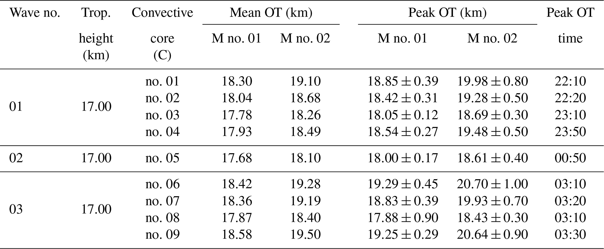
It is important to note that the error in the propagation time of the ray path was estimated from the mesopause to tropopause, considering three different ray tracing paths from three different starting positions on the first visible CGW crest. The maximum error estimated in the propagation times was ±24 min. These three different ray tracing starting positions were considered to study the influence of the wind on each ray path in several directions to give a general idea of the possible source locations. Considering the error, three CTBT images before and after 23:27 UT were used to track the overshooting in time unless the core being tracked dissipates rapidly. This rapid dissipation of a core within the given time range can be seen in the case of C no. 03, where there was no overshooting after 23:40 UT. In such a case, the 20 min remaining in the forward tracking time was added to the reverse tracking time, setting the starting time to 22:40 UT. In Table 2, the details of the overshooting tops – the waves, convective cores, average overshooting heights, peak overshooting heights, and the time of the overshooting – are summarized. The results were obtained using the method of Griffin et al. (2016) (M no. 01) and São Sabbas et al. (2010) (M no. 02). Now let us consider the positions of these Cs in space at these time stamps.

Table 2 Characteristics of overshooting tops (OTs) of the convective cores (Cs) during the 1–2 October 2019 CGW events.

Before tracking the convective cores in space, the error of the CGW propagation in space was considered. This kind of estimation is important because it helps to verify the wind's effect and approximate the most likely source position of the wave. The error in space and time was estimated similarly, where three different ray tracing paths from three different starting positions on the first visible CGW crest were used. It is done to estimate and define the region within which the overshooting convective cores will be considered. We demonstrate here how this computation was performed using the case of Wave no. 01, as shown in Fig. 9.

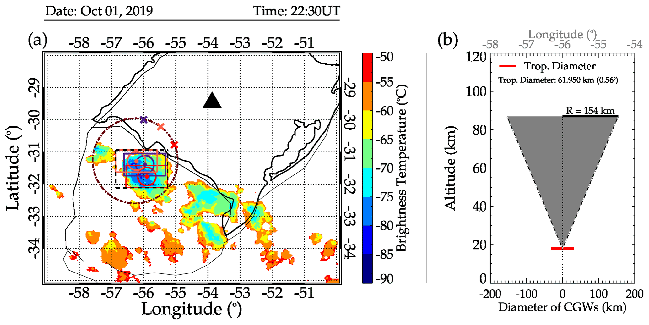
Figure 9 A pictorial description of how the regions of overshooting convective cores were considered to determine the overshooting tops tracked in space and time.

Figure 9a shows the map of the CTBT image at 22:30 UT, the cross symbols depict the positions where the ray tracing began, and the dashed–dotted circle shows the first visible concentric crest to appear in the OH image. Each color of the “×” corresponds to the circles of the same colors, which were constructed from the tropopause diameters. The rectangle was constructed using the diameter and the estimated errors in longitude and latitude in the ray paths (zero and model winds). The dashed black rectangle was constructed from the extreme positions of the three rectangles. Figure 9b is the pictorial description of how the diameter of the tropopause was estimated. The “radius (R) = 154 km” above the horizontal line extending from the middle (the vertical dotted lines) shows the radius of the cone in 2D at the OH emission altitude.

The black triangle, cross symbols (“×”), and dashed–dotted circle are the same as in Fig. 4a. Each color of the “×” corresponds to their respective circles with center (filled circles) and rectangles. The vertical dashed black lines depict the height of the cone with radius (R). This radius is the same as the radius of the first visible concentric structure in the OH images. The horizontal solid red line indicates the diameter of the tropopause, and the vertical slanted dashed black and white lines extending vertically at either side of the dotted line are used to restrict the propagation of the CGWs above the tropopause after the overshooting of the tropopause.

To determine the tropopause diameter, the concept of a conical propagation configuration of CGWs was used (Vadas et al., 2009b; Nyassor et al., 2021). The base of the cone with a radius (same as the radius of the CGWs) of 154 km was set at 87 km of altitude. We then followed the slant heights of the cone, determining the radius at each kilometer until we reached the vertex of the cone. The vertex of the black and white dashed line–slanted path is above the tropopause. Certainly, the radius of the CGW at the vertex right above the overshooting top is zero. However, it is important to determine the diameter of the tropopause because this is the region within which overshooting may occur.

According to Vadas et al. (2009a, 2012), a typical diameter of a convective plume is 15–20 km. So, we consider first the dome-like protrusion shooting from the highest overshooting point to the anvil of the cloud. Then, we set a cloud top temperature threshold of −70 ^∘C and constructed a circle with a radius of ∼31 km around the pixel with the coldest CTBT. The −70 ^∘C thresholds were set because it was observed that other protrusions (or overshootings) do originate from CTBT within this BT range every 10 min. So, to restrict the selection of OTs to the spatial resolution of 2 km plus ∼4 km (2 extra pixels), we set the diameter of the overshooting region to be the diameter of the tropopause. The extra 4 km is added to have a full view of CTBT that may appear in 2 pixels. Determining the diameter of the tropopause is crucial because it is used to approximate possible regions within which overshooting is most likely to occur.

Next, we constructed rectangles around each circle using the diameter of the tropopause as shown in the Fig. 9a. To construct each respective rectangle, the estimated error in longitude (latitude) of the model wind ray path of the wave is added to the zonal (meridional) (i.e., right and left – up and down) sides of each circle. The estimated errors in longitude and latitude of Wave no. 01 (Fig. 4a) are ±40 and ±7 km, respectively. Finally, the dashed black rectangle was constructed from the extreme points of the respective individual rectangles. The overshooting convective cores within the dashed black rectangle were considered for tracking the overshooting tops. A similar procedure was applied to the other two CGW events to determine their respective region within which the overshooting convective cores were considered. Now we track Wave no. 01 in space.

The peak OTs of C no. 03 and C no. 04 for Wave no. 01 and their occurrence time fell within the error range when the ray path of the wave reached the tropopause. Here, we track the OTs in space as shown in Fig. 10. The symbols used to indicate the trajectory of the OTs in Fig. 10 are the same as in Fig. 8, except for the open squares and circles with black outlines that indicate the position of the OT at the time of the CTBT map. The closed squares with black outlines show the position of the OT of the preceding CTBT map in the previous time. The time stamps of each CTBT map are presented in the upper left corner in each panel. Note that the time stamp with the black background highlights the wave excitation time estimated by the ray tracing model. The stopping and tropopause positions of the model wind ray path are depicted by the blue circle and star, respectively, whereas the red circle and star represent that of the zero wind model. As defined earlier in Fig. 4, the cross is the wave crest, whereas the diamond is the center of CGW, represented by the dashed–dotted dark-red circle.

Figure 10 Tracking of the individual convective cores (Cs) no. 01, no. 02, no. 03, and no. 04 in space and time for Wave no. 01.

Tracking these overshooting tops in space, we observed that the OT positions of C no. 03 and C no. 04 of Wave no. 01 were far from the determined center and the ray path position at the tropopause. The closest core to the CGW center and the ray path tropopause position was C no. 03 and 50 km away. This core first overshot at 22:40 UT (open white circle with black outline in Fig. 10f). C no. 03 was active till 23:40 UT. For C no. 04, the first overshooting occurred at 23:00 UT and ∼100 km away from the CGW center and the tropopause position (the red open circle with black outline in Fig. 10h). Following Cs no. 03 and no. 04, we observed that both cores presented OT at the excitation time, that is, at 23:30 UT (see Fig. 10k). However, their OT heights corresponding to this time showed overshooting < 1 km in Fig. 8. Therefore, there is a low probability of these cores exciting Wave no. 01. Between 22:40 and 23:10 UT and at 23:40 UT for C no. 03 and at 23:50 UT for C no. 04 (see Fig. 8), we observed overshootings > 1 km, but the positions of these cores in space were quite distant from the excitation location (see Fig. 10f–l).

It is worth noting that Wave no. 01 was visible in the first airglow image of the night, implying this wave had already reached the OH airglow layer before the observation started. Hence, the exact time the wave first appeared in the OH image could not be obtained. So, despite these two cores (i.e., C no. 03 and C no. 04) overshooting more than 1 km (see Fig. 8 and Table 2 for the peak OT heights) and also not knowing the exact time the wave first appeared on the airglow image, these OTs could possibly not be the source of Wave no. 01. Also, the time when the peak OT altitude of C no. 04 occurred was after the estimated time when the ray paths of Wave no. 01 reached the tropopause. Even if the wave first appears in the OH images at 00:27 UT, this further strengthens the fact that C no. 04 (red open circle with black outline) cannot be the source of Wave no. 01.

Not knowing the exact time when Wave no. 01 first appeared makes it challenging to identify the approximate source position and time using the ray tracing model. Since no significant overshooting by the cores was observed after 23:50 UT, we tracked the cores back in time and space. Two other convective cores, C no. 01 and C no. 02, were observed with higher OTs within the hours of 21:50 and 23:00 UT and 21:50 and 23:20 UT, respectively (clearly observed in Fig. 8). C no. 01 had large OT variations during the entire time the core was active, with a peak OT altitude of 18.85 km at 22:10 UT (see Fig. 8). In Fig. 10c this OT in space is close to the CGW center and the tropopause position. Also, temporal variations were observed in the profile of C no. 02 in Fig. 8, especially within the hours of 21:50 and 22:30 UT, with a peak OT altitude of 18.42 km at 22:20 UT. However, the position of this peak OT in space is distant from the CGW center and the tropopause position, that is, the open orange square with a black outline at a time stamp of 22:20 UT (Fig. 10d).

Tracking Cs no. 01 and no. 02 in space, we observed that the distributions (of dark-red and orange squares with black outlines) for these two OTs were much closer to the ray-traced determined source locations of Wave no. 01, especially C no. 01. Considering the variations observed in the OTs (C no. 01 and C no. 02 in Fig. 8), their peak OT altitudes, time of peak OT, and their distributions in space around the identified source locations showed these two convective cores are the most likely cores that overshot to excite Wave no. 01. Note that before 21:50 UT, no other active convective cores were seen within the error ranges in longitude and latitude considered.

3.4.3 Tracking Wave no. 02 in space and time

The tracking of Wave no. 02 in space is presented in Fig. 11. Wave no. 02 first appeared on the OH airglow images at 00:55 UT and disappeared around 01:07 UT. However, the backward ray tracing result showed that the ray path of this wave reached the tropopause at around 00:15 UT (Fig. 11a). The cloud top temperatures of the system between 00:10 and 00:30 UT were hotter than the tropopause temperature, which signifies that the convective cores present within this time frame were not overshooting. From Fig. 8 and Table 2, it is shown that C no. 05 overshot at 00:50 UT with a peak OT altitude at 18.00 km (i.e., ∼1 km). Other OTs of C no. 05, besides the one at 00:50 UT, overshot less than 1 km. In space, this overshooting is ∼140 km away from the wind model tropopause position and ∼220 km away from the determined center, as shown in Fig. 11e.

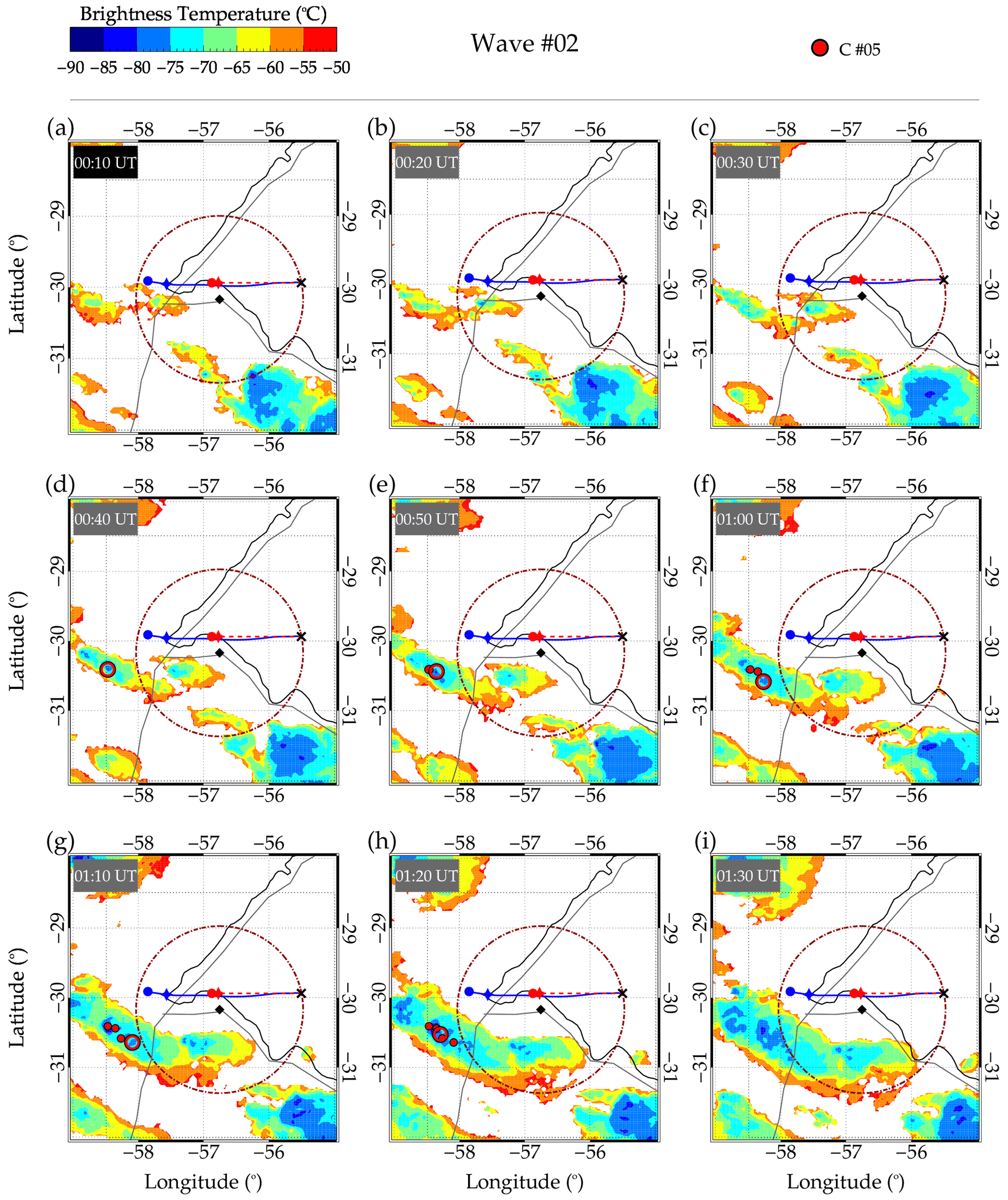
Figure 11 Tracking of the individual convective core (C), C no. 05, in space and time for Wave no. 02.

Further analysis on the time of the peak OT altitude showed that this overshooting could not be responsible for the generation of Wave no. 02, if the wave was first visible at 00:55 UT in the OH images and the highest overshooting occurred at 00:50 UT. This wave could not propagate to the OH emission layer within 5 min, considering the temporal scale of the wave. Since the identified source was not overshooting when the ray path reached the tropopause and did not have active convective cores ±30 min within the error range in longitude and latitude, this wave could be excited by another mechanism. Since other GW generation mechanisms are out of the scope of the current work, this wave will be left for further investigation in future work.

3.4.4 Tracking Wave no. 03 in space and time

In Fig. 12, it is seen that the OTs observed in the CTBT maps centered around the estimated source position of the Wave no. 03 are tracked in space at each time stamp of the GOES observation from 02:10 to 04:00 UT. Here, we examine the details of the convective cores (Cs) of Wave no. 03. In Fig. 12, it is seen that, similar to Wave no. 01, Wave no. 03 has four convective cores, C no. 06, C no. 07, C no. 08, and C no. 09. The red and orange squares with black outlines represent OTs of C no. 06 and C no. 07, whereas the OTs by C no. 08 and C no. 09 are depicted by the white and red circles with black outlines, respectively. For C no. 06, C no. 07, and C no. 09, variations in the OT altitudes were observed, as shown in Fig. 8.

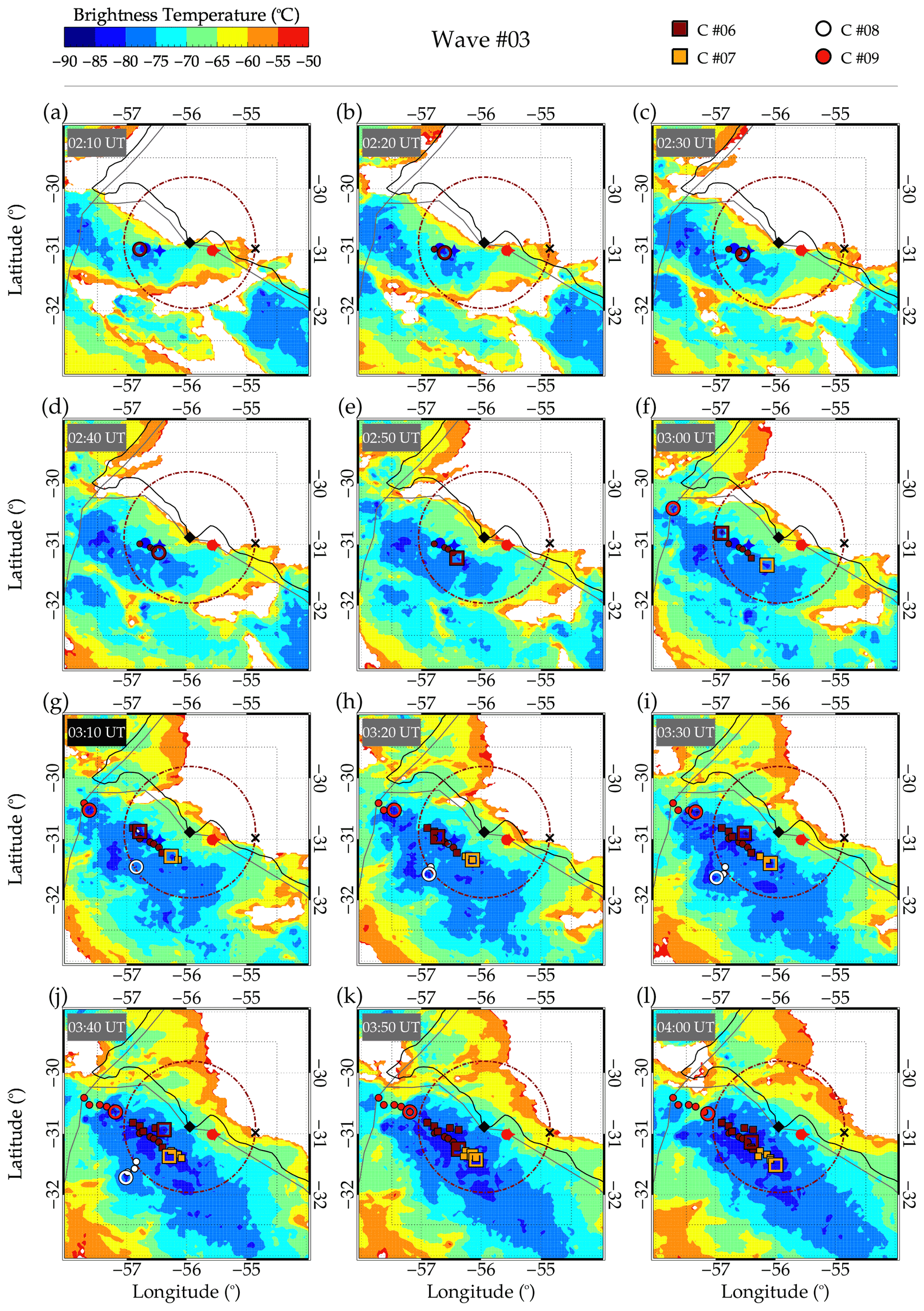
Figure 12 Tracking of the individual convective cores (Cs), C no. 06, C no. 07, C no. 08, and C no. 09, in space and time for Wave no. 03.

The peak OT altitudes of C no. 06, C no. 07, and C no. 09 occurred at 19.29, 18.83, and 19.25 km and 03:10, 03:20, and 03:30 UT, respectively. Interestingly, the ray tracing results showed that the ray paths of the model wind reached the tropopause at 03:10 UT, whereas the ray path of the zero wind model reached the tropopause at 03:20 UT. This indicates the estimated excitation times of Wave no. 03. At the model-wind-estimated excitation time (i.e., 03:10 UT), the positions of C no. 06 and C no. 07 in Fig. 12g were found close to the tropopause position of the model wind results (i.e., the blue star). On the other hand, the position of C no. 06 and C no. 07 in Fig. 12h, corresponding to the estimated excitation time (i.e., 03:20 UT) of the zero wind, were also close to the model wind tropopause position (i.e., the blue star).

It was observed that the OT of C no. 06 at 03:20 UT is much closer to the model wind tropopause position than the OT at 03:10 UT (see the open dark-red squares with black outlines in Fig. 12g and h). The lifetime of an overshooting event, according to Cooney et al. (2018) and Nyassor et al. (2021), spans ∼5–10 min. So, considering the fact that (a) the GOES-16 CTBT images have a temporal resolution of 10 min, and (b) the MCS with the convective cores were moving, it is possible that the OT captured in Fig. 12g and h might be the same since no significant displacement can be observed in the position. This indicates that either of these OTs of C no. 06 can excite Wave no. 03, with the OT of C no. 06 at 03:10 UT (Fig. 12g) having a greater probability of exciting Wave no. 03. This is because the OT height at this time is higher than the OT height at 03:20 UT (see Fig. 8).

Figure 13 A combined plot of tracked individual convective cores/overshooting tops of Wave no. 01 with Cs no. 01, no. 02, no. 03 and no. 04, Wave no. 02 with C no. 05, and Wave no. 03 with Cs no. 06, no. 07, no. 08, and no. 09 in space and time. In the upper panels (a)–(c), the Cs are plotted over the map with the CTBT map at each wave event excitation time and the wind vector, whereas the lower panels (d)–(f) are the wind magnitude and vector. The wind corresponds to the hour in which the waves were excited. The arrows show the direction of the wind at the tropopause.

Even though the time of peak OT altitude of C no. 09 (red circles with black outline) was within the error range, the spatial distribution of this core was found outside of (a) the first visible concentric crest and (b) the error range in longitude and latitude. Therefore, C no. 09 has a lower probability of being the OT that excited Wave no. 03. Also, C no. 08 (white circle with black outline) was outside the error range in longitude and latitude. The temporal variation in the OT altitudes of C no. 08 had a peak altitude of 17.88 km at 03:20 UT. The peak altitudes of C no. 08 and C no. 07 co-occurred. However, with C no. 07 having ∼0.93 km OT altitude higher than C no. 08 and also closer to the source location (tropopause position), C no. 08 cannot be the overshooting that generated Wave no. 03.

Between 02:10 and 02:40 UT, the OTs of C no. 06 are represented by the dark-red circles with black outline in Figs. 8 and 12. Even though these OTs were out of the error range in time, their spatial distribution was centered close to the tropopause position of the wind model ray path. Therefore, they were included to verify if these OTs significantly overshot. No significant overshooting was observed, except for the OT at 02:20 UT. However, this OT cannot be the source of Wave no. 03 because it occurs ∼40 min before the estimated excitation time of this wave. The time difference is similar to the propagation time of Wave no. 03 from the tropopause to the OH altitude.

It is important to mention that the tracking approach used by São Sabbas et al. (2009) to track convective cores relative to lightning discharges was adapted to identify the most likely convective cores that generate the three CGWs. In this study we adapted the method because the MCS during this night was moving southeastward at an average speed of ∼18 m s⁻¹. At the tropopause, the horizontal wind obtained from the European Centre for Medium-Range Weather Forecasts (ECMWF) model showed that the wind was southeast throughout the three CGW events. The vector plot of the wind direction is overlaid on the CTBT map, and the wind magnitude is shown in Fig. 13.

All the symbols in Fig. 13 have the same meaning as explained in each wave event. Figure 13 shows that the wind at the tropopause was towards the southeastern direction throughout the entire period of the wave events. The magnitude of the wind (Fig. 13d–f) at the tropopause is shown by gray contours. From Fig. 13, it can be noted that the MCS and wind direction agree with each other. Also, the average wind speed during the CGW events is similar to the speed of the MCS.

As mentioned earlier, two methods were used to estimate the overshooting tops: (i) Griffin et al. (2016) (M no. 01) and (ii) São Sabbas et al. (2010) (M no. 02). The results of the two methods, presented in Fig. 14, show that the OT altitudes estimated by both techniques agree since the error bars overlap. The error in both methods was estimated by calculating the propagation error of each point. The propagation error estimation in the positions and times of the wave trajectory follow the procedure of Bevington and Robinson (2003). As shown in Fig. 14, the maximum estimated errors are $\sim \pm \mathrm{0.6}$ km and $\sim \pm \mathrm{0.9}$ km for the methods of Griffin et al. (2016) (M no. 01) and São Sabbas et al. (2010) (M no. 02), respectively.

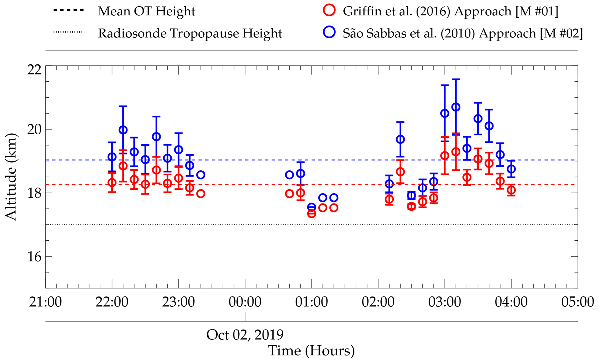
Figure 14 Comparison between the two OT altitude estimation methods. OT altitudes in red circles represent the Griffin et al. (2016) method, whereas the São Sabbas et al. (2010) method is represented by blue circles. The black dotted lines depict the radiosonde tropopause height, and the mean OT height is shown by the dashed lines. Red represents the Griffin et al. (2016) method and blue the São Sabbas et al. (2010) method.

3.5 Other severe weather-associated events

Other severe weather-associated events such as intense lightning activities, hail, and transient luminous events (TLEs) were observed during the CGW events. The lightning activities were recorded by the Brazilian Lightning Detection Network (BrasilDAT) sensors. Using the same technique employed in Nyassor et al. (2021), the locations with the highest lightning densities were found to coincide with the location of the coldest cloud tops (overshooting tops), as shown in Fig. 15. The lightning densities were obtained by binning the positions of the lightning strike into $\mathrm{0.06}{}^{\circ }\times \mathrm{0.06}{}^{\circ }$ (6.6 km × 6.6 km) grid boxes. A comparison between the spatial distribution of the lightning strikes and the CTBT of the MCS showed a direct relationship between the two phenomena. Several studies, for example, Medeiros et al. (2003), Wrasse et al. (2003), Xu et al. (2015), and Nyassor et al. (2021), showed the relationship between GWs/CGWs and deep convection. Xu et al. (2015) observed strong lightning activities during the summer, where many CGWs were observed.

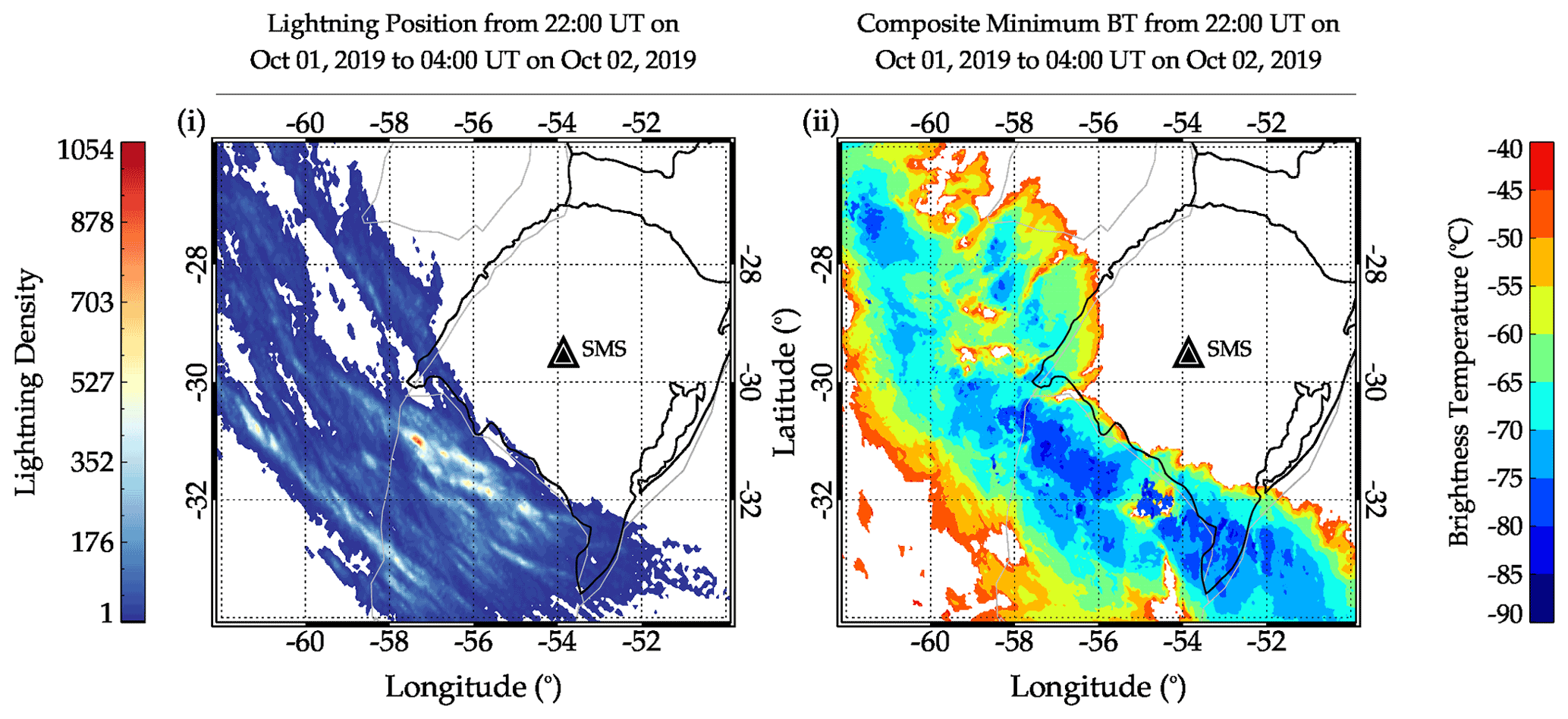
Figure 15 Comparison between the spatial distribution of lightning density and composite GOES-16 IR cloud top brightness temperature images from 22:00 UT on 1 October 2019 to 04:00 UT on 2 October 2019. The filled black triangle within a white triangle shows the location of the Southern Space Observatory.

In a CGW study, Yue et al. (2013) observed lightning flashes around the center of the typhoon-generated CGWs. The point-like source of convective CGWs, that is, overshooting of the tropopause, has been related to strong updraft activities within deep convection. Nyassor et al. (2021) and references therein showed the direct relationship between the intensity/density of lightning activities in space and overshooting tops of deep convection by the strong updraft. Nyassor et al. (2021) further found that regions with a high density of spatial distribution of lightning agree with the coldest regions of the CTBT. Previous studies by Bedka et al. (2010) demonstrated that CTBT greater than 200 K or less than −73.15 ^∘C has a higher occurrence of lightning activities within 10 km around the overshooting tops. In Fig. 15, it was observed that lightning activities have high densities in regions where the CTBTs are very cold, indicating overshooting tops.

Several transient luminous events (TLEs), especially sprites, were also observed during these CGW events. Here we report the observation of two sprite events registered with the LEONA TLE station installed at the Southern Space Observatory (SSO). The first event occurred at 00:42:28 UT and the second one at 00:46:51 UT on 2 October 2019. Both events are shown in Fig. 16.

Figure 16 Image of two groups of sprites generated by the same thunderstorm that generated the CGWs observed during the night of 1 to 2 October 2019.

Sprites are short-duration plasma discharges and low-intensity optical emissions observed at night. They are generated by the quasi-electrostatic field established by charge extinction within the thunderstorm resulting from lightning discharges, predominantly of positive cloud-to-ground (+CG) lighting. In the upper atmosphere above cloud tops (at ∼12–20 km altitude), this field extends all the way to the base of the nighttime ionosphere, at ∼100 km altitude, where it is strongly shielded by the ionospheric plasma. When a lightning discharge extinguishes enough charge inside the thunderstorm, free electrons present in the atmosphere between the cloud tops and the ionosphere can be accelerated by its quasi-static field and gain enough energy to start an electron avalanche process at ∼70–85 km altitude, which may initiate one or several plasma streamers that may form a sprite or a group of sprites. Thus, sprites initiate at ∼70–85 km altitude, and their streamers can extend down to as low as ∼30 km and up to ∼100 km at the base of the nighttime ionosphere (São Sabbas et al., 2010). Therefore, sprites pierce right through the airglow layer, at ∼87 km altitude. Their lateral dimensions can be a few tens of meters in the case of column sprites and up to ∼40 km in the case of carrot sprites (São Sabbas et al., 2010, and references therein).

Both sprite events reported here are groups of column sprites with thin columns, possibly a few tens of meters thick. The first event displayed one well-defined long column with two dark bands, an intense bead at the bottom, and several very faint diffuse columns on its left side. The second event was composed of at least 10 short columns, two very bright and the rest diffuse, all showing a broader diffuse region on the top, called hair, which is typical of carrot sprites and not very common on column sprites. This report is the first observation of sprites and gravity waves in South America.

Sprites and CGWs have been simultaneously observed once before, by Sentman et al. (2003), in the central region of the United States during a field campaign in 1999. Using low-light intensified CCD cameras, Sentman et al. (2003) observed at least 12 bright sprites above a mesoscale convective system over the state of Nebraska for a period of 2 h during which they also observed concentric gravity waves generated by the same MCS using a 25 s exposure CCD fitted with a red filter. The estimated wave periods and wavelengths were ∼10 min and ∼50 km, respectively, during the first hour of observation and ∼11 min and ∼40 km, respectively, during the second hour. They used the well-established optical intensity of ∼1 kR for the observed OH Meinel emission. They compared it to the intensities of the observed sprite to estimate an upper limit to the thermal energy deposited by sprites in the mesosphere, reaching the value of ∼1 GJ. Since a detailed TLE analysis and comparison with the gravity wave observations is not the focus of the current study, future work will further explore the combined observations of these phenomena. These events are presented in the current work to emphasize the severity of the convective activity before, during, and after the CGWs' observation.

4 Summary and conclusion

Three concentric gravity wave (CGW) events excited by a mesoscale convective system on the night of 1 to 2 October 2019 were studied. A ray tracing model was used to identify the source positions of the CGW events. The moving of the MCS required the development of a new method to identify the most likely OTs that excited the observed CGW. This method employed the tracking of the OTs in space and time.

The identified sources (OTs) for Wave no. 01 and no. 03 showed high overshooting tops within the spatial and temporal ranges determined within the error margin in space and time. However, the exact time when Wave no. 01 first appeared in the OH images was unknown since the wave was present in the first OH image of the night. Further analysis of the source of Wave no. 01 by tracking the OTs back in time showed that Wave no. 01 was most likely excited around 22:20–22:40 UT on 1 October 2019, by either C no. 01 or C no. 02. This is because C no. 01 and C no. 02 were closer to the expected source location estimated by the ray tracing and the determined center. On the other hand, the identified source of Wave no. 02 did not coincide with any convective core with significant overshooting. The peak OT altitude of C no. 05 of Wave no. 02 occurred 5 min before the wave was first seen in the OH image. Analyzing the characteristics of Wave no. 02, the wave could not have propagated to the OH altitude within 5 min; hence it is unlikely that C no. 05 was the source of Wave no. 02. For Wave no. 03, the OT by C no. 06 at 03:10 UT is considered the most probable core that excited this wave.

The estimation of the tropopause height was not straightforward for the days analyzed in this work; the tropopause was colder than what is usually observed and reported in literature. This colder tropopause could be a consequence of cooling of the upper troposphere due to the presence of this intense MCS or the presence of Rossby waves or quasi-horizontal flow or some other large-scale upper tropospheric process driven by extratropical dynamics. Therefore, the tropopause determination procedure adapted differed from the approach used by Nyassor et al. (2021, and references therein). We average the vertical temperature profiles of 12 d, including days with and without convection and starting 2 d prior to the day of the CGW events. From that we established an average tropopause for those days that we used as a reference to estimate the overshooting vertical extent of the convective cores identified as possible sources of the observed CGWs. Radio occultation temperature profiles from nine locations, where the gravity waves were generated and observed, were analyzed to complement the radiosonde measurements when estimating the tropopause temperature and height.

Since this study investigates a moving source of CGWs through overshooting convective cores in a MCS moving approximately 18 m s⁻¹, the convective cores with OTs were tracked in space and time in order to identify the most likely sources. It is important to mention that this method aims to identify the exact source of waves excited through the oscillator mechanism of deep convection. It is, therefore, possible to adapt and apply this method in the investigation of sources of convective generated GWs.

Appendix A: Radio occultation temperature profiles observed from 1 to 3 October 2019

To verify the variations in the tropopause height and temperature observed in the radiosonde observation (Fig. 7 in the main text), the radio occultation temperature profiles were used. For the plots shown in Fig. A1, only profiles taken from 1 to 3 October are presented. There were no simultaneous observations of radiosonde and radio occultation temperature profiles on the other days. To produce Fig. A1, the closest profiles within a radius of ∼400 km centered around the center of each CGWs are selected. For each of the days used in this plot, only three sounding profiles were found within this set region.

Figure A1a–c show the radio occultation observation on 1–3 October 2019. For each panel (i.e., Fig. A1a–c), (i) shows the tropopause temperature variations along the time of sounding, (ii) presents the contour plot of the three profiles for each day from 0–60 km, and the sounding positions of the profiles are shown in (iii). In Fig. A1d, the individual profiles of the three soundings selected for each day, 1, 2, and 3 October, are presented. As defined in the legends, the red-scale squares in Fig. A1a(iii) correspond to the profiles in Fig. A1d(i), blue-scale squares in Fig. A1b(iii) correspond to the profile in Fig. A1d(ii), and gray-scale squares in Fig. A1c(iii) correspond to profiles in Fig. A1d(iii). The square with the black or gray outline indicates the start time of the sounding position. The time range of the soundings is written in the corresponding colors of the squares representing the sounding positions. In Fig. A1a(ii), b(ii), and c(ii), the dashed white lines with the dots show the variations in the tropopause height.

Even though the data set is not evenly distributed in space and time, it could be observed in Fig. A1d that the profiles for the set of data for each day are similar. From Fig. A1a(i), b(i), and c(i), it is shown that the variations in the profile showed increasing tropopause temperature through the days similar to the radiosonde observation. For the variations in the tropopause height in (ii) of Fig. A1a–c, no distinct variation was observed. The average tropopause height is 17.29 km. Despite mentioning earlier that the data point in space and time is irregular, it was considered in this analysis because the focus here is to study the general behavior of the variations in the tropopause temperature. In summary, a similar trend in the variations of the tropopause temperature was observed on the same days of observations in both radiosonde and radio occultation data.

Figure A1 Radio occultation sounding profiles around the SMS observatory from 1 to 3 October 2019 before, during, and after the CGW event.

Appendix B: Larger view of the MCS around São Martinho da Serra with respect to the observed CGW

Figure B1 Same as panels (a(i))–(c(i)) of Fig. 4 in the main article but an extended coverage with the cloud top brightness temperature ranging from 0 to −90 ^∘C. Panels (a), (b), and (c) represent Wave no. 01, Wave no. 02, and Wave no. 03, respectively.