Sixteen years of MOPITT satellite data strongly constrain Amazon CO fire emissions

Despite the consensus on the overall downward trend in Amazon forest loss in the previous decade, estimates of yearly carbon emissions from deforestation still vary widely. Estimated carbon emissions are currently often based on data from local logging activity reports, changes in remotely sensed biomass, and remote detection of fire hotspots and burned area. Here, we use 16 years of satellite-derived carbon monoxide (CO) columns to constrain fire CO emissions from the Amazon Basin between 2003 and 2018. Through data assimilation, we produce 3 d average maps of fire CO emissions over the Amazon, which we verified to be consistent with a long-term monitoring programme of aircraft CO profiles over five sites in the Amazon. Our new product independently confirms a long-term decrease of 54 % in deforestation-related CO emissions over the study period. Interannual variability is large, with known anomalously dry years showing a more than 4-fold increase in basin-wide fire emissions relative to wet years. At the level of individual Brazilian states, we find that both soil moisture anomalies and human ignitions determine fire activity, suggesting that future carbon release from fires depends on drought intensity as much as on continued forest protection. Our study shows that the atmospheric composition perspective on deforestation is a valuable additional monitoring instrument that complements existing bottom-up and remote sensing methods for land-use change. Extension of such a perspective to an operational framework is timely considering the observed increased fire intensity in the Amazon Basin between 2019 and 2021.

1 Introduction

The role of Amazon forests in supporting biodiversity, regional ecosystem services, and carbon storage (Gloor et al., 2012) is threatened by human activity, in the form of large-scale deforestation (Davis et al., 2020) and climate change. In Brazil specifically, various studies suggest that, in recent years, deforestation rates and associated fire activity are once again accelerating (INPE, 2020; Pereira et al., 2020), after having reached a minimum around 2012 (Yin et al., 2020). Moreover, recent droughts in 2010 and 2015–2016 led to maxima in biomass burning (Silva Junior et al., 2019). Reliable monitoring of fire activity and its impacts provide objective detection and mapping of deforestation, which helps in investigating underlying drivers. Such information is key for developing efficient mitigation measures and for reducing fire risks.

Monitoring fires primarily relies on remote sensing products such as burned area (Giglio et al., 2018), fire radiative power (FRP), and fire counts (Giglio et al., 2016). Such products can be combined with pre-burn fuel load, emission factors, and combustion completeness to estimate fire emissions of different species (Wiedinmyer et al., 2011; van der Werf et al., 2017; Kaiser et al., 2012). Rapid and continuous processing of vast amounts of such data allowed recent unexpectedly high fire activity in 2019 to be detected and reported quickly (Lizundia-Loiola et al., 2020; Brando et al., 2020). However, fire dynamics are complex, and products based on land remote sensing data are prone to miss small fires (Randerson et al., 2012; Ramo et al., 2021), are hampered by cloud cover (Schroeder et al., 2008), and might be poorly able to detect understory fires (Morton et al., 2013). Understory fires in particular contribute strongly to forest fragmentation and mortality, and they can increase forest vulnerability to burning (Nepstad et al., 2001; Alencar et al., 2004). In addition to the direct detection of fire activity, information is needed to quantify the corresponding carbon loss to the atmosphere on scales from decades to seasons as well as from the entire Amazon Basin down to individual Brazilian states.

During fires, a combination of pollutants is released into the atmosphere, the composition of which depends on local fire conditions but generally includes a large contribution from carbon monoxide (CO). With an atmospheric lifetime of 1–3 months, CO is not well mixed globally; hence, fire emissions produce large and, thus, easily detectable enhancements over the CO background concentration. Therefore, enhancements in CO over and around the Amazon Basin can provide information on the frequency, intensity, and location of fires. Moreover, the CO released from fires that escaped direct detection, such as under cloud cover or in the understory, can still be detected. Finally, CO fire emissions can be linked to total carbon emissions and emissions of other pollutants with the use of emission factors (e.g. Ferek et al., 1998; van Leeuwen et al., 2013), providing insight into the climate and air quality impacts of fires.

Satellite CO data are especially useful for quantifying and mapping fire emissions, due to their temporal and spatial detail as well as their availability in remote areas. In this work, we focus on the use of satellite-detected CO column retrievals from the Measurement Of Pollution In The Troposphere (MOPITT) instrument (Deeter et al., 2019), which is an established product for CO emission quantification (Jiang et al., 2017; Miyazaki et al., 2020). For the Amazon Basin specifically, MOPITT CO data have previously been analysed to show that a long-term decrease in deforestation over the 2002–2016 period is partly counteracted by large fires in drought years (Aragão et al., 2018; Deeter et al., 2018).

Here, we move beyond direct analysis of satellite data and incorporate these data into the TM5-4D-Var (Krol et al., 2005; Meirink et al., 2008) data assimilation system. By linking satellite data to the TM5 3D transport model, we can map and quantify CO fire emissions in the Amazon with improved detail and accuracy. The long time series of MOPITT CO satellite data has previously been used in data assimilation studies for estimating the global CO budget (Zheng et al., 2019), also with a focus on fire emissions (Yin et al., 2020). Other data assimilation studies that have been focused on South America have provided insight into fire and drought events over shorter time periods (Hooghiemstra et al., 2012; van der Laan-Luijkx et al., 2015). This study adds value to previous work by providing a focused and rigorous analysis of fire emissions in the Amazon over a long time period (2003–2018), which adds context to both global studies and studies that focused on shorter time periods.

We first present fire emissions over the entire Amazon Basin (Sect. 3.1.1); we then zoom in on individual Brazilian states (Sect. 3.1.2) as well as on different land-cover types (Sect. 3.1.3). This level of detail helps to better understand and quantify differences between bottom-up and top-down estimates as well as to assess anthropogenic and natural contributions to fire emissions. An important asset of our analysis is a detailed investigation of the uncertainties in the Bayesian inverse system. To this end, we investigate the influence of components such as the prior fire CO emission inventory, natural production, and loss fields, and we additionally assimilate a different satellite product. Uniquely, we independently assess our MOPITT-based emission estimates as well as those from the Global Fire Assimilation System (GFAS) bottom-up inventory, using a multi-year CO record from an aircraft whole-air flask sampling network in the basin (Sect. 3.2.2) (Gatti et al., 2014, 2021).

2 Methods

2.1 Transport model

We operate the TM5 atmospheric transport model (Krol et al., 2005) at a global resolution of  4^∘ × 6^∘ (latitude ×longitude). We additionally use the zoom capability of the TM5 model to include two nested regions over South America, in a set-up similar to van der Laan-Luijkx et al. (2015) (see Fig. 1). The inner zoom domain (red grid in Fig. 1), with a 1^∘ × 1^∘ resolution, spans longitudes from 75 to 39^∘ W and latitudes from 28^∘ S to 8^∘ N. The outer zoom domain (green grid in Fig. 1), with a 2^∘ × 3^∘ resolution (latitude × longitude), spans longitudes from 84 to 30^∘ W and latitudes from 34^∘ S to 14^∘ N. Note that we present most results for the inner zoom domain only. All regions are operated with 25 vertical layers, covering the range from surface pressure to top of the atmosphere, typically with 3–6 model layers in the planetary boundary layer. Transport in TM5 is driven by 3-hourly, offline meteorological fields from the European Centre for Medium Range Weather Forecasts (ECMWF) ERA-Interim reanalysis (Dee et al., 2011), which have a native resolution of approximately 80 km with 60 vertical layers.

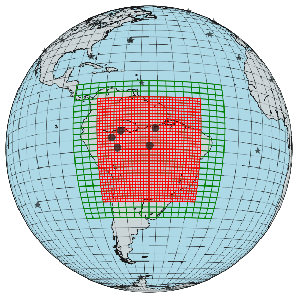
Figure 1 A map of the South American zoom regions used in the TM5 simulations. The green and red grids indicate the 3^∘ × 2^∘ and 1^∘ × 1^∘ (longitude × latitude) zoom regions respectively. Over both zoom regions, satellite data are assimilated. Filled stars indicate the NOAA Global Greenhouse Gas Reference Network surface sites, from which surface observations are assimilated to constrain global CO emissions, and, by extent, the boundary conditions of the zoom domains. Filled circles indicate sites where discrete whole-air samples were collected by aircraft at various altitudes. The CO data calibrated on whole-air samples are used for independent evaluation of the inversions.

2.2 Prior source and sink fields

We performed 2003–2018 inversions with three prior fire inventories: the Global Fire Assimilation System (GFASv1.2; Kaiser et al., 2012), the Fire INventory (FINNv1.5) from the National Center for Atmospheric Research (NCAR; Wiedinmyer et al., 2011), and a climatological (i.e. annually repeating) prior based on the average emission distribution in GFAS (hereafter referred to as CLIM). The GFAS emission distribution is provided at a 0.1^∘ × 0.1^∘ resolution, and the FINN distribution is available at a resolution of ∼1 km × 1 km; however, we regrid both to our coarser model resolution. GFAS and FINN use different data from the Moderate Resolution Imaging (MODIS) satellite as a proxy for the global, daily fire distribution: GFAS uses fire radiative power (FRP), whereas FINN uses active fire counts. Both inventories overlay these proxies with land-cover maps from the MODIS instrument, and they employ land-cover-specific emission factors for CO (and other species) to produce the emission estimates that we use. However, the exact land-cover classifications and emission factors used differ between the two inventories. We use the inversions that start from the GFAS prior as a reference, and we discuss the differences between the fire priors where relevant.

Fire emissions retrieved in our inverse system are informed by both the prior emission distribution (e.g. GFAS) and the assimilated observational data (e.g. MOPITT). To assess the importance of either component, we have constructed a climatological prior (CLIM) that includes no interannual variability nor spatial gradients. As such, variability in the posterior emissions retrieved in the CLIM inversions is driven exclusively by the assimilated CO data and atmospheric transport. As we optimize CO fire emissions at a 3 d resolution (Sect. 2.6), we also construct the CLIM prior at a 3 d resolution. We construct the CLIM prior as follows: (1) we average the daily CO emission fields from GFAS over the 2003–2018 period; (2) if the total CO emissions in a grid cell are less than 0.03 Tg during a 3 d period, the emissions in that grid cell and 3 d window are set to zero; and (3) the 3 d total fire emissions inside the 1^∘ × 1^∘ zoom domain are divided uniformly over those grid cells that initially had emissions higher than 0.03 Tg. In this way, approximately 24 % of the inner domain grid cells still contain emissions. We choose this approach to prevent spatial gradients in the GFAS estimate from influencing posterior emissions; the approach is balanced by the 0.03 Tg lower limit to retain some potential to recover high, localized emissions from the CLIM prior. Outside the $\mathrm{1}{}^{\circ }\times \mathrm{1}{}^{\circ }$ zoom domain, the CLIM prior still includes interannually varying GFAS emissions.

All fire emissions (GFAS, FINN, and CLIM) are distributed vertically in the simulations following vertical emission profiles derived in the Integrated System for wildland Fires (IS4FIRES) (Soares et al., 2015). In contrast to the horizontal emission distribution, the vertical emission distribution does include diurnal variability. In a sensitivity test, we have found that including a diurnal cycle in only the vertical emission distribution produces results that are comparable to including diurnal variability in both the horizontal and vertical distribution of CO fire emissions (results not shown). Therefore, we do not impose sub-daily variability on the native daily resolution of GFAS and FINN emissions in the simulations.

For the chemical production of CO from methane (CH₄) and from non-methane volatile organic compounds (NMVOCs), we use fields generated in a 2006 simulation in the full-chemistry version of TM5 (Huijnen et al., 2010). We use anthropogenic CO emissions from the Monitoring Atmospheric Composition and Climate CityZen (MACCity) inventory (Lamarque et al., 2010). The annually repeating, monthly hydroxyl radical (OH) concentration fields are a combination of tropospheric OH fields from Spivakovsky et al. (2000), scaled by 0.92 as recommended in Patra et al. (2011), and stratospheric OH fields derived in the 2D Max Planck Institute for Chemistry (MPIC) chemistry model (Brühl and Crutzen, 1993). In Sect. 3.3.3, we discuss the sensitivity of the inversion results to the chemical CO production and to the OH distribution.

2.3 Satellite retrievals

In the reference inversions, we assimilate CO column retrievals from version 8 of the Measurements Of Pollution In The Troposphere (MOPITT) instrument (Deeter et al., 2019) over both South American zoom domains. MOPITT retrieves CO columns using both the CO absorption band in the thermal infrared (TIR) at 4.7 µm and in the near-infrared (NIR) at 2.3 µm. In this work, we only use CO columns retrieved in the TIR band. MOPITT has a swath of 22 km × 650 km, with 116 cross-swath pixels, and daily overpass times of 10:30 and 22:30 LT (local time) each morning and night for the inner zoom domain. Following Nechita-Banda et al. (2018), we inflate column errors reported by the MOPITT team by a factor $\sqrt{\mathrm{50}}$ to compensate for the high number of satellite data (∼10 000 d⁻¹ in both zoom domains combined) relative to the number of surface observations (∼150 per month; see also Sect. 2.4). CO columns are sampled from the transport model using the MOPITT averaging kernels.

In Sect. 3.3.1, we present inversions in which satellite data from the Infrared Atmospheric Sounding Interferometer (IASI) instrument (Clerbaux et al., 2009) are assimilated instead of MOPITT. IASI retrieves CO columns exclusively in the TIR waveband, with a 12 km × 4 km footprint at nadir. Identical versions of the IASI instrument fly aboard three operating platforms (Metop-A, -B, and -C), but we limit ourselves to the Metop-A data in this work, which cover the longest time period. Importantly, while IASI and MOPITT exploit similar wavebands, they use different measurement techniques (George et al., 2015). The overpass time of IASI typically precedes the MOPITT overpass time by 1 h. Importantly, different from MOPITT, we only assimilate IASI daytime data.

2.4 Surface observations

To constrain global emissions of CO outside of the model zoom domains, we assimilate CO mole fraction observations from the surface whole-air flask sampling network (40–45 sites) of the NOAA Global Greenhouse Gas Reference Network (GGGRN) (Petron et al., 2019). We use a fixed observational error of 2 ppb CO per flask pair average, with no model error. We choose not to adopt a model error for surface observations, as this would only require further inflation of the error in satellite data (see above). We test the effect of reducing this observational error to 0.2 ppb CO in Sect. S1 in the Supplement.

2.5 Aircraft observations

We use a set of aircraft observations over the Amazon for independent validation of the inverse results over the 2010–2017 period. Atmospheric air samples were collected at a range of altitudes over five sites in the Brazilian Amazon (Gatti et al., 2014, 2021). The Tabatinga site (TAB) was replaced by Tefé (TEF) in 2013, and we generally group these two sites in our analysis. Site locations are indicated in Figs. 1 and 6. The sampling flights were performed using small aircraft, typically two times per month, between 12:00 and 13:00 LT, in a descending helicoidal profile that avoids sampling emissions from the aircraft. One profile typically includes 12–17 air samples between 300 and 4500 m a.s.l. (metres above sea level) (Gatti et al., 2014, 2010). The concentrations of the aircraft samples have been analysed by the National Institute for Space Research (INPE; São José dos Campos, Brazil) LaGEE (greenhouse gas laboratory) since 2015; before 2015, they were processed at the Nuclear and Energy Research Institute (IPEN) in an atmospheric chemistry laboratory in São Paulo. LaGEE uses standards calibrated against the World Meteorological Organization reference scales maintained by the NOAA Global Monitoring Laboratory (i.e. the same calibration scale that is used for NOAA GGGRN surface observations). In the period during and after this transition (2015–2016), operation of the aircraft network was partly interrupted (see also the right-hand column in Fig. 6). A 2010–2013 subset of these aircraft data was previously used for direct validation of MOPITT CO data (Deeter et al., 2016). However, as we sample both satellite and aircraft data from a 3D-simulated atmosphere, our validation more realistically accounts for the different vertical sensitivities of the two datasets.

2.6 Optimization procedure

We employ the TM5-4D-Var inverse system (Meirink et al., 2008) to optimize CO emissions between 2003 and 2018 in 16 separate inversions, which each cover the April–December period of 1 year (i.e. centred on the Amazon fire season). Simulating 9 instead of 12 months greatly improves the speed of convergence of the inversions, as the complexity of the inverse problem scales non-linearly with the number of assimilated observations and optimized state elements. Because Amazon fires occur mostly between June and November, this set-up still provides us with a 1 month spin-up and spin-down period.

Figure 2 Prior and posterior fire CO emission estimates summed over the 1^∘ × 1^∘ South American zoom domain (see Fig. 1). Panel (a) presents the May–December total emissions per year. Panel (b) shows the monthly total emissions, with the colours distinguishing prior (green) from posterior (orange) and the line style indicating the prior used. Shaded areas mark the spread between the three priors and the three posteriors respectively. Note that the posterior estimates mostly overlap; thus, these are visible as one line only.

The CO satellite data are only assimilated inside both zoom domains over South America. In the zoom domains, we optimize 3 d total CO fire emissions, with a relative grid box error on the emissions of 250 %, a horizontal correlation length of 200 km, and a temporal correlation of 3 d. Total emissions in the global domain are constrained mainly from NOAA surface observations, and they are optimized with a prior uncertainty of 250 % as well as with a horizontal and temporal correlation of 1000 km and 9.5 months respectively. Emissions are optimized non-linearly, following a semi-lognormal distribution, to prevent negative posterior emissions, as in Bergamaschi et al. (2009). Because the 4D-Var system does not produce posterior error covariance matrices for a non-linear system, we instead explore the uncertainties of the inverse system in sensitivity tests (e.g. adjusting the prior emission distribution, adjusting the observational errors, and assimilating a different satellite product; see Sects. 3.3, S1, and S2).

3 Results

3.1 Flux analysis

3.1.1 Basin-wide Amazon fire emissions

The inverse system retrieves annual total (May–December) fire emissions that vary strongly interannually (Fig. 2a): from 26 Tg CO in 2018 to 127 Tg CO in 2005. Typically, GFAS, FINN, and the posterior estimates show the highest and lowest emissions in the same years. However, the posterior interannual variability is significantly larger (standard deviation of 34 Tg CO yr⁻¹) than the prior variability (standard deviation of 19 Tg CO yr⁻¹). We find that, averaged over 2003–2018, GFAS emissions need to be increased by 50 % to match MOPITT CO data, with the largest underestimates in dry years (e.g. by 130 % in 2015). For FINN, the average underestimate is smaller at 20 %.

The spread between posterior estimates that start from different emission priors is significantly smaller (standard deviation of 2 Tg CO yr⁻¹) than the spread between prior estimates (standard deviation of 12 Tg CO yr⁻¹). The strong posterior agreement between inversions is an especially noteworthy result for the CLIM prior, which does not include any interannual variability. This result shows that the posterior variability is almost exclusively driven by MOPITT data and TM5 transport, rather than by prior information from the fire inventories. Therefore, we consider that the overall agreement between the prior and posterior interannual variability shows that the fire inventories are generally very able to identify high-emission years.

The fire emissions show a strong seasonal cycle (Fig. 2b), with low emissions in April–May and December in most years, in both the prior and posterior emission estimate. This finding generally supports the use of a 9-month inversion period, and it confirms that treating April and December as respective spin-up and spin-down months does not strongly affect the annual total CO fire emissions.

Figure 3 Interannual variability in the area-average soil moisture and fire CO emissions in five Brazilian states. The four outside panels (a, c, d, e) show the 2003–2018 time series of May–December total CO emissions from biomass burning (left axis, in orange and green) and the annual averaged root-zone soil moisture from the Global Land Evaporation Amsterdam Model (GLEAM v3.3a) product (right axis, in blue), for five Brazilian states. A year is defined here as June–December (i.e. centred on the dry season). Both prior (green) and MOPITT-optimized (orange) fire CO emissions are shown, for the three inversions that start from different prior fire inventories (indicated by solid, dashed, and dot-dash lines). Shaded areas indicate the spread between the fire inventories before (green) and after (orange) the inversion. Also shown at the top are the correlation coefficients (R² values) between CO emissions and soil moisture for the optimized emissions from the inversion that start from the GFAS inventory. Maranhão and Tocantins are combined, as they are smaller states that represent similar regimes in terms of climate and anthropogenic activity. Note the different y scales between the four figures, with the lowest emissions in Amazonas. Panel (b) shows a map of these five Brazilian states.

In this 16-year record, 2015 is the year that breaks from these general conclusions. Firstly, while it does not show up as a high-emission year in GFAS and FINN, it does show up as a high-emission year in all posterior estimates. Additionally, it is the only year with high emissions in November and December. Therefore, it is possible that the 2015 estimate is affected by spin-down effects and that we miss emissions in early 2016. However, in an inversion from November 2015 to May 2016, we find that the January 2016 emissions are low and that December 2015 emissions are not significantly affected by extending the inversion window (results not shown).

3.1.2 Fire emissions in Brazilian states

We have quantified interannual variability in fire CO emissions for five Brazilian states to assess these emissions at a sub-basin scale (green and orange lines in Fig. 3). As an indicator of relative drought between years, we have also shown the local root-zone soil moisture anomalies, as provided by the Global Land Evaporation Amsterdam Model (GLEAM v3a; Miralles et al., 2011; Martens et al., 2017; blue lines and right y axes in Fig. 3). Mato Grosso and Pará make up most of the Brazilian “Arc of Deforestation”, and Maranhão and Tocantins (grouped in our analysis) are on the edge of it. Amazonas represents a more pristine area in the Amazon Basin. Together, these five states cover most of the Brazilian Amazon.

We find a strong link between interannual variability in optimized CO fire emissions and local soil moisture anomalies. Interannual variations in CO emissions are markedly different per state, and years with low soil moisture levels generally show high fire emissions. For example, the 2010 fires are mostly located in Mato Grosso, while the 2015–2016 fires are concentrated in Pará and Maranhão/Tocantins, coinciding with local negative anomalies in soil moisture. The GFAS and FINN prior emissions are similarly anticorrelated with soil moisture. However, we also find a similar correlation for the CLIM inversions (result not shown), which do not include prior interannual variability. This result confirms that our inverse set-up can retrieve state-level interannual variability independent of prior assumptions. Moreover, especially in 2015, emissions are strongly adjusted in the inversion, and this coincides with local negative soil moisture anomalies.

We have quantified the correlation between the optimized GFAS emissions and soil moisture anomalies, and we find that it is significant for all states, at a significance level of p=0.05 (correlation coefficients per state are shown in Fig. 3). The correlation coefficients are largely insensitive to the averaging approach for soil moisture (e.g. selecting the annual minimum value or averaging over fewer months). Previous work has already established a strong link between fire emissions and soil moisture (e.g. Asner and Alencar, 2010; Silva et al., 2018), but the strength and consistency of the anticorrelation that we find here, at the level of individual states, is noteworthy. Of course, drought is not the only determinant of fire emissions, and in Sect. 3.1.3 we explore the role of deforestation.

Similar to the basin-wide emissions (Fig. 2), we find that the spread between posterior estimates at the state level is much reduced compared with the spread between prior estimates. The posterior estimates do not only agree with respect to their interannual variability but also regarding the spatial allocation of the emissions between states. For example, the GFAS emissions in Amazonas are on average 4 Tg CO yr⁻¹ lower than the FINN emissions; however, after the inversion, the estimates converge to the lower GFAS estimate, with a much smaller residual difference between the two posterior estimates of 1 Tg CO yr⁻¹. This shows that not only are the Amazon total fire CO emissions well constrained by the inversions but their spatial allocation are also well constrained.

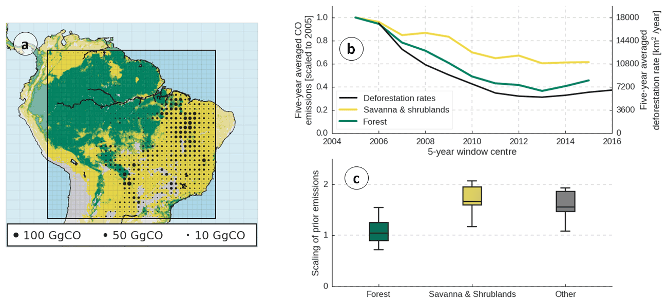
Figure 4 Spatial allocation of emissions between land-cover types as well as the long-term trends in the emissions. Panel (a) presents a land-cover map of South America, with land-cover types retrieved from the MODIS product, at a 0.1^∘ × 0.1^∘ resolution. We distinguish between forest (green) and savanna–shrublands (yellow). Grid cells covered by less than 70 % of both are shown in grey. The map covers the 3^∘ × 2^∘ zoom region used in TM5, and the black outline indicates the 1^∘ × 1^∘ zoom region, which is the focus of our study. The area of the black circles is proportional to how much CO is added to the GFAS prior emissions in the inversion, over the 2003–2018 study period (see also legend). Panel (b) provides a time series of the 5-year averaged annual total CO emissions from biomass burning over the 1^∘ × 1^∘ TM5 zoom domain for two land-cover types: forest (in green) and savanna–shrublands (in yellow). Emission totals are scaled to the emissions in the first 5-year window (see the left y axis), which is centred on 2005. Also shown are the 5-year averaged deforestation totals (black, right y axis), as retrieved from the Brazilian Amazon Deforestation Monitoring Program (PRODES). Note that the area used for PRODES deforestation rates is different from the forest mask that we use for emission attribution, as PRODES (among other differences) only quantifies deforestation in Brazil. Panel (c) presents a box plot that shows how much annual total emissions over each land-cover type are adjusted through optimization with MOPITT satellite data. This can be compared to the black circles in panel (a).

3.1.3 Long-term trends and land-cover type

We observe a significant downward trend in the MOPITT-derived CO emissions over our full inner zoom domain (Fig. 4b), which is largely insensitive to the prior inventory used in the inversion. We focus here on 5-year averaged emissions in order to visualize the clear downward trend that is otherwise partly masked by interannual variations in emissions (e.g. Fig. 3). We disaggregate the trend between forests and savanna, based on Version 6 of the annual land-cover data from the MODIS Land Cover Climate Modeling Grid (CMG) (Fig. 4) (Sulla-Menashe et al., 2019). We find that the decrease over the study period (between the fire CO emissions averaged over 2003–2007 and over 2014–2018) is larger over forest (∼54 %) than over savanna and shrublands (∼39 %), and the stronger trend over forests is matched in magnitude and sign by a decrease in the independently derived estimates of deforestation from the Brazilian Amazon Deforestation Monitoring Program (PRODES; INPE, 2020). The PRODES deforestation rates quantify the area deforested each year that has not been deforested before. Notably, both deforestation rates and fire emissions have stopped decreasing since ∼2012. Deforestation, especially the narrow definition used in PRODES, does not always overlap with fires – for example, when fires occur in reforested areas, or when cut forest is burned with delay or not at all. However, most fires are in some way caused by local anthropogenic activity, for which deforestation is a good proxy. The close match in trends shows that fire abatement policies do reduce fire emissions, but this is often masked by interannual, drought-driven variations. This conclusion confirms similar assessments in earlier MOPITT-based work (Aragão et al., 2018; Deeter et al., 2018); however, here, with the use of the TM5-4D-Var inverse system, we are able to quantify both the decrease and drought-driven interannual variations.

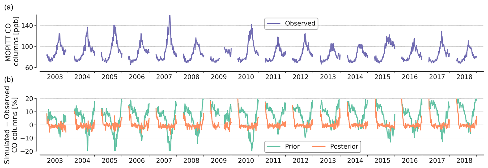
Figure 5 A comparison between simulated and MOPITT-retrieved CO columns for the GFAS reference inversion. Panel (a) shows the TM5-simulated and MOPITT-retrieved CO columns, averaged over the inner 1^∘ × 1^∘ zoom domain and at a 3 d time resolution. Note that the posterior simulation and the MOPITT-retrieved CO columns largely overlap; thus, the latter is poorly visible. Panel (b) presents the relative difference between satellite-retrieved and simulated MOPITT CO columns, in a simulation with the prior GFAS emissions (green) and after the MOPITT CO column retrievals have been assimilated to optimize fire emissions (orange), averaged as in panel (a). The difference between the simulated and observed columns is quantified as a percentage of the average satellite-retrieved CO column.

The prior CO emissions from both GFAS and FINN are too low to reproduce MOPITT CO column retrievals in all years, for all land-cover types, but the underestimate is much stronger over savanna and shrublands than over forests (Fig. 4c and black circles in Fig. 4a). A strong systematic underestimate over savanna–shrublands is indicative of underestimated CO emission factors and carbon stock, as other explanations (such as missed small fires or understory fires) are more likely to impact emission estimates from forests. We do note that the amplitude of the underestimate over savanna–shrublands (median of 67 %) is large compared with typical uncertainties in emission factors (e.g. van Leeuwen et al., 2013) and carbon stock. As noted earlier, we find that emissions in dry years, such as 2010 and 2015, are more strongly underestimated than emissions in wet years. We find that the FINN and GFAS inventories underestimate fire emissions most strongly in 2015, which could, in part, be driven by the timing of these fires. The 2015 fires continued into November and December (see Sect. 3.1.1): months that typically have more cloud cover, which inhibits direct fire detection.

3.2 Comparison to observations

In this section, we assess the skill of our prior and posterior simulations to reproduce the assimilated satellite data as well as independent aircraft profiles of CO. A comparison with surface observations is presented in Sect. S1. Results presented in this section are largely insensitive to the prior fire inventory used, which is why we only present results from the reference GFAS inversions.

3.2.1 MOPITT satellite retrieval

The MOPITT-retrieved CO columns show a distinct seasonal cycle that peaks in September in most years (Fig. 5a), similar to the fire emissions (Fig. 2). In the prior simulations, we find significant differences between the domain-averaged simulated and satellite-retrieved CO columns (Fig. 5b). In the posterior, these differences are reduced to less than 2 % of the observed columns. The 9-month inversion window does show a spin-up period of approximately 1 month in which the difference is larger, as we do not optimize the initial CO distribution. The posterior agreement between the simulations and the MOPITT data confirms that, with adjustments to biomass burning emissions inside the zoom domains and with adjustments to total emissions outside of the domains, we can reproduce satellite-retrieved MOPITT CO columns in our simulations within their observational errors.

Differences between simulated and observed columns in the prior simulation are indicative of the types of adjustments in CO emissions that are needed to reproduce observed columns. Firstly, simulated CO columns outside of the dry season are systematically too high (by about 8 %–15 %). Secondly, superimposed on this systematic overestimate, we find that the peaks in CO column retrievals during dry season are underestimated in the prior simulations. We largely attribute the overestimate to overly high secondary production of CO (as further discussed in Sect. S2.1). Because we do not optimize secondary production in our inversion, the overestimate is largely corrected by adjusting emissions outside the inner zoom domain, which are only loosely determined by the NOAA surface observations (see Sect. S1). The prior underestimate of the dry-season peak in CO is most likely related to fire emissions, and we indeed find that fire emissions are increased after data assimilation (Sect. 3.1.3).

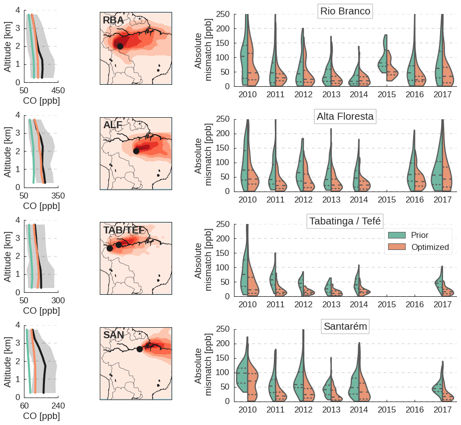
Figure 6 Comparison between simulated and observed aircraft profiles over five sites in the Amazon. Profiles sampled over Tabatinga and Tefé are combined, as they represent similar air masses and have complementary temporal coverage (Tabatinga up to 2013 and Tefé after 2013). The profiles cover the 2010–2017 period, and we have included only profiles sampled between August and November. The left column presents the time-averaged (2010–2017) simulated (prior in green; posterior in orange) and observed (black) aircraft profiles, binned in 500 m intervals. The grey shaded areas show 1 standard deviation of the variability between the individual observed aircraft profiles. The centre column shows maps of the influenced area of each site or each site combination. Black dots indicate site locations, and the red area indicates the origin of air at the site location. Red areas are proportional to the logarithm of the number of back trajectories that originate at the sampling location and altitude, and then pass through a grid cell, as determined from simulations in the Hybrid Single-Particle Lagrangian Integrated Trajectory (HYSPLIT) model (Stein et al., 2015). Further details are provided in Gatti et al. (2010). Back trajectories from the Lagrangian grid in the HYSPLIT model were interpolated to the TM5 1^∘ × 1^∘ grid. The right column presents violin plots of the absolute difference between observed and simulated aircraft samples of CO, in a simulation with GFAS-optimized (green) and in a simulation with MOPITT-optimized biomass burning emissions (orange). The dashed lines inside each violin indicate the median and the two inner quartiles.

3.2.2 Validation with aircraft profiles

Whole-air flask sampling flights were conducted over five sites in the Amazon Basin between 2010 and 2017 (Gatti et al., 2021). We compare the TM5-simulated CO mole fractions to those measured from the samples of vertical profiles (Fig. 6). This independent validation clearly shows an improved overall match after the assimilation of the MOPITT-retrieved CO columns. In simulations with prior GFAS emissions, we find a site-averaged bias of −62 ppb, which decreases to −19 ppb after the optimization (visible in the left-hand columns of Fig. 6). This improvement confirms that the prior GFAS emissions are too low to reproduce observations. For Santarém, the residual bias is largest (−32 ppb CO after optimization), but MOPITT CO column retrievals over the same region are matched well after optimization (Sect. S3). We do find a significant absolute residual error between simulated and observed aircraft profiles, which can be explained by the relatively coarse resolution of the transport model (1^∘ × 1^∘ with 25 vertical layers; see Sect. 2.1), which puts a limit on how well individual aircraft samples can be represented in TM5. However, we find that the MOPITT-derived emissions generally greatly improve the agreement with independent aircraft profiles at the five different locations across the Amazon, compared with the GFAS prior. This gives us confidence in the fact that our inversion improves estimates of CO emissions from fires across different regions of the Amazon Basin – for example, for different Brazilian states (Sect. 3.1.2).

3.3 Sensitivity tests

3.3.1 Assimilating IASI instead of MOPITT satellite data

We have performed additional inversions in which we assimilate CO column retrievals from the IASI Metop-A instrument (Clerbaux et al., 2009). We find that MOPITT-derived emissions are slightly higher than IASI-derived emissions before 2014 (6–12 Tg CO yr⁻¹), whereas IASI-derived emissions are significantly higher than MOPITT-derived emissions (15–30 Tg yr⁻¹) after 2014 (see Fig. 7). Within each of these two time periods, the difference between interannual variability in IASI- and MOPITT-derived emissions is small (∼10 Tg yr⁻¹) relative to this jump (∼30 Tg yr⁻¹).

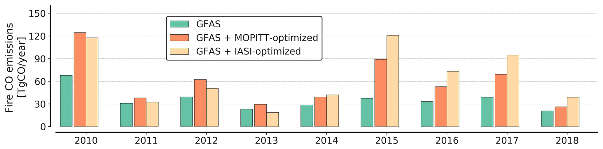
Figure 7 Total CO emissions from biomass burning summed over the $\mathrm{1}{}^{\circ }\times \mathrm{1}{}^{\circ }$ South American zoom domain and over the April–December inversion period. Results for two sets of inversions are shown, which each started from the GFAS fire prior: the first is the default inversion that used MOPITT satellite data, and the second used IASI satellite data.

We have sampled MOPITT columns in simulations with IASI-optimized biomass burning emissions to investigate the timing of this jump (Fig. 8). Over 2010-2013, simulated MOPITT CO columns are in good agreement with those retrieved by MOPITT, which indicates consistency between the MOPITT and IASI records. However, a jump occurs in 2014, after which simulated MOPITT columns become biased high, which is consistent with the difference in emissions. The onset of this bias of around 8 % occurs instantaneously on 30 September 2014, as indicated in Fig. 8. Over the 2010–2018 period, several changes have been made to the IASI retrieval that can cause inconsistencies (e.g. Table 2 in Bouillon et al., 2020), and a major update to the processing algorithm that was implemented on 30 September 2014 apparently has a particularly large impact on the retrieved CO columns. Based on the coincidence of these two events, we consider the switch in IASI–MOPITT offset to be an artefact in the IASI data record.

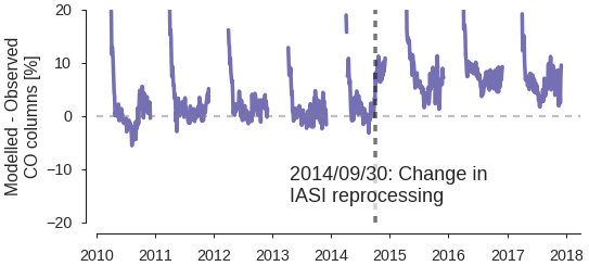
Figure 8 The difference between satellite-retrieved MOPITT CO columns and MOPITT CO columns sampled in a simulation that used CO emissions optimized with IASI-retrieved CO columns, over the 1^∘ × 1^∘ South American zoom domain. The difference is quantified as a percentage of the satellite-retrieved CO columns. The date on which IASI switches between two meteorological datasets (30 September 2014) is indicated; on this date, a jump in the difference between simulated and satellite-retrieved MOPITT CO columns occurs.

We conclude that as long as the IASI retrieval does not use a consistent meteorological dataset, the retrievals before and after 30 September 2014 are best treated as two separate data records. Currently the IASI team is finalizing a full reprocessing of the CO Metop-A record, using the ERA5 reanalysis as input for temperature profiles in order to generate a homogeneous record. The resulting consistent IASI product will provide better grounds for an uncertainty estimate of the driver satellite data, which is currently more difficult to perform. We do consider the relative consistency in interannual variability between IASI and MOPITT, except for the 2014 break, evidence of the robustness of interannual variability in CO emissions derived from either satellite product. The systematic difference between MOPITT and IASI is a measure of the systematic uncertainty in the satellite data and its impact on derived annual total fire CO emissions, which amounts to 10–30 Tg yr⁻¹ for the inner zoom domain.

3.3.2 Integrated comparison to Zheng et al. (2019)

We have additionally compared our derived CO emissions to those derived by Zheng et al. (2019). Their emission estimate, covering 2000–2017, was derived in an inversion that also assimilated MOPITT TIR CO column retrievals. However, that is the only shared aspect of our two inverse set-ups. Their inversion assimilated MOPITT CO column retrievals globally, which will result in different boundary conditions for the Amazonian domain than assimilation of surface observations. Additionally, their inversion was performed at a different spatial resolution (1.9^∘ × 3.75^∘, latitude × longitude, with 39 vertical layers) in a different transport model (LMDz-SACS; Pison et al., 2009). As a prior for fire CO emissions, they used emissions from version 4.1s of the Global Fire Emissions Database (GFED) (van der Werf et al., 2017). Prior OH fields used in Zheng et al. (2019) were the same as ours, but theirs were optimized with methyl chloroform surface observations. Additionally, they used biogenic CO  emissions from the Model of Emissions of Gases and Aerosols from Nature (MEGANv2.1) inventory, which, as discussed in Sect. S2.1, differ significantly from those used in our inversions. Further details on their inverse set-up are provided in Table 1 of Zheng et al. (2019). We limit our comparison to emissions derived in Inversion 1, as described in Zheng et al. (2019), in which satellite retrievals of formaldehyde and methane were not assimilated.

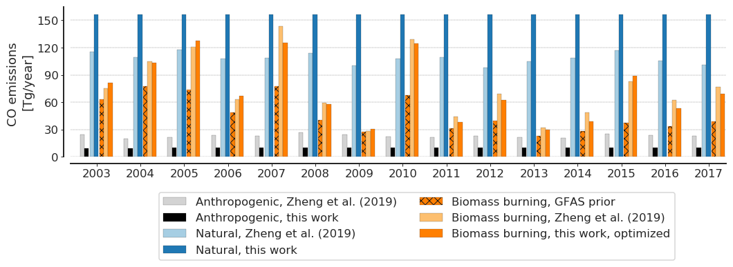
Figure 9 Emission totals for different source categories from this work, compared to emissions from Zheng et al. (2019). Total CO emissions are summed over the $\mathrm{1}{}^{\circ }\times \mathrm{1}{}^{\circ }$ South American zoom domain as well as over the April–December inversion period. For bars corresponding to this work, emissions from our standard inversion are shown (i.e. GFAS fire emissions optimized with MOPITT-retrieved CO columns) as well as emissions from a global MOPITT inversion performed by Zheng et al. (2019). Emission categories from Zheng et al. (2019) were merged to obtain emission categories comparable to ours.

We find that biomass burning emissions derived in Zheng et al. (2019) are comparable to ours, both with respect to absolute magnitude and to interannual variability (orange bars in Fig. 9), with an average annual total difference of $-\mathrm{3.0}\pm \mathrm{6.7}$ Tg CO yr⁻¹ (1 standard deviation). This difference is small compared with interannual variability. Notably, their emission estimates of CO from biomass burning are also systematically higher than those from GFAS and FINN. Different from our inversions, the MEGANv2.1 inventory for biogenic emissions includes interannual variability, and these emissions are significantly lower than the biogenic emissions that we have used (see also Fig. S3). The excellent agreement between these two largely independent estimates provides much confidence in the final emission estimates.

3.3.3 Other sensitivities in the inverse system

We have additionally explored the sensitivity of derived emissions to other individual components of the inverse system, which are presented in detail in Sect. S2. Here, we briefly summarize the main conclusions from these sensitivity tests. We find that natural production of CO from non-methane volatile organic compounds (NMVOCs) is the largest sensitivity in our inverse system (Sect. S2.1), with an associated systematic uncertainty in derived fire CO emissions of 23–27 Tg yr⁻¹. The associated uncertainty in the interannual variability in fire CO emissions is 10–15 Tg yr⁻¹. We additionally find a large sensitivity to the OH sink of CO, but we attribute this mostly to unrealistically low OH values in the fields from the Copernicus Atmospheric Monitoring Service (CAMS) reanalysis that we use for the sensitivity test (Sect. S2.2). Finally, we find that if we reduce the error on NOAA surface observations, we retrieve a better posterior match with these data, without changing the derived fire emissions. This result indicates limited sensitivity to boundary conditions as determined by surface observations that are sampled mostly outside the domain in which we assimilate satellite data.

Overall, we conservatively estimate the uncertainty in the interannual variability in the MOPITT-derived CO emissions of biomass burning at 10–15 Tg CO yr⁻¹, and the systematic uncertainty is estimated at 30 Tg CO yr⁻¹, which is dominated by production from NMVOCs. We consider this uncertainty estimate conservative because the integrated comparison with Zheng et al. (2019) suggests a lower uncertainty of 7 Tg CO yr⁻¹ (Sect. 3.3.2). A small uncertainty is somewhat intuitive, as fire emissions are uniquely sharp in location and timing, and this signal is well captured in the MOPITT data. Therefore, fire emissions are only partly interchangeable with other, typically more diffuse budget components.

3.4 Discussion

The robustness of derived emissions signifies the detail provided by the MOPITT TIR product. In addition to the TIR product, MOPITT also provides an NIR product and a combined NIR–TIR product. The NIR product has relatively higher vertical sensitivity near the surface. Due to its range of spectral bands, MOPITT data can be used to separately constrain upper- and lower-tropospheric CO (Deeter et al., 2018). Here, we have limited our analysis to the TIR product, which already provides strong constraints on CO fire emissions. Nechita-Banda et al. (2018) showed that the TM5-4D-Var inverse system produces similar fire emissions when MOPITT TIR or NIR–TIR are assimilated over Indonesia. Peiro et al. (2022) performed a global CO inversion with MOPITT NIR–TIR data and found South American fire emissions that were typically lower than ours. Therefore, in future work, it would be interesting to investigate the added value of NIR in the NIR–TIR product in more detail. Additionally, we use MOPITT version 8, but the newer MOPITTv9 version has recently become available (Deeter et al., 2022). Importantly, the changes made in the retrieval result in significantly improved coverage over areas with high aerosol concentrations, which are also emitted in fires. Clearly, improved coverage near fires will strongly benefit our inverse analysis, and future work can benefit from these improvements.

Our fire emission estimates rely strongly on the quality of the MOPITT CO retrieval. The MOPITT CO data have been validated extensively (Deeter et al., 2016, 2019), and we again present a good agreement with independent aircraft profiles in this work. Other CO satellite products are available that can complement a MOPITT-based analysis. Firstly, we presented a comparison to inversions that use IASI instead of MOPITT CO data (Sect. 3.3.1). This comparison reveals inconsistencies in the reprocessing used for IASI, but the interannual variability derived from the two products within the 2010–2013 and 2015–2018 periods is similar. A consistently processed IASI product, which is something that the IASI team is finalizing, will help better assess the MOPITT-derived emissions. Additionally, an expanding fleet of satellite instruments is becoming available, which monitor atmospheric composition with increasing detail. This can help with cross-validation, and new satellites, such as the TROPOspheric Monitoring Instrument (TROPOMI; Borsdorff et al., 2018), also have higher spatial resolution, providing a potential step forward in the level of detail with which fire emissions can be inferred (van der Velde et al., 2021). We do note that we draw value from the long-term availability and consistency of the MOPITT product in this work, which is something that other products currently cannot compete with.

An important application of top-down estimates of CO fire emissions is to propagate these to CO₂ fire emissions so that the Amazon carbon balance can be better constrained. In previous work, this has been done by directly applying CO : CO₂ emission factors from bottom-up inventories to the updated CO emissions (van der Laan-Luijkx et al., 2015; Peiro et al., 2022). In our case, this would mean that the CO₂ fire emissions over the Amazon in the GFAS and FINN inventories would be scaled up, as we find that CO emissions in these inventories are underestimated. Whether this approach is appropriate strongly depends on the driver of the underestimate we have found. Scaling up the CO₂ emissions based on our CO inversion is appropriate if the underestimate of CO fire emissions is related to missed understory fires (Alencar et al., 2004) or to an underestimate in carbon stock. However, if the underestimate is related to errors in the CO emission factors (van Leeuwen et al., 2013), the total carbon emissions reported in the bottom-up inventories could still be accurate. As a first indication, we find that the underestimate in GFAS is largest over savanna and shrubland regions, which makes it less likely that understory fires are a dominant driver. A recent study has shown that a combined analysis of satellite data of CO and NO_x can provide top-down constraints on combustion efficiency and emission factors (van der Velde et al., 2021). Additionally, a burned-area analysis of high-resolution Sentinel-2 data over Africa concluded that missed small fires in GFED4s might result in a 31 % underestimate of fire carbon emissions (Ramo et al., 2021). The updated version of the FINN fire inventory (v2.5; Wiedinmyer et al., 2022) also increases fire CO emissions in the Amazon Basin by 102% (averaged over the 2003–2018 period) compared with the version used in this work (v1.5; Wiedinmyer et al., 2011). These new developments show that there is perspective on reconciling our top-down estimates with bottom-up efforts, which can be further informed by the spatio-temporal patterns of the higher emissions that we derive.

An operational framework that estimates CO fire emissions based on satellite-retrieved CO columns and prior information (e.g. FRP) can provide unique and timely information about regional variability in fires. CAMS already provides an operational data assimilation framework in which, among other data products, MOPITT TIR CO column retrievals are assimilated (Flemming et al., 2017). We identify two aspects in which the CAMS analysis can be improved. First and most importantly, the atmospheric abundance of CO is optimized in the CAMS system, instead of CO emissions. We suggest that a next development of a CAMS-like system should consider emission optimization for a more physically realistic end product that can be used to provide information on variations in sources, such as in Miyazaki et al. (2020). Second, we show that the CAMS OH fields produced in full-chemistry simulations are very low over the Amazon, which other studies have indicated is due to incomplete NO_x sources (Wells et al., 2020) or incomplete chemical mechanisms (e.g. Lelieveld et al., 2008; Taraborrelli et al., 2012). Such an underestimate in OH can mask the GFAS underestimate that we find here, which has important implications for the interpretation of fire emissions. Operational CO emissions can provide a rich proxy for fire variability and deforestation. Moreover, the immediate context provided by a long-term, consistently derived time series of CO emissions is highly valuable for interpretation of recent fire events. This would be timely, considering that recent changes in the natural and political climate surrounding the Amazon (INPE, 2020; Silva Junior et al., 2020; Fonseca et al., 2019) necessitate active fire monitoring by as many independent proxies as possible.

4 Conclusions

In this study, we present a 2003–2018 time series of fire CO emissions in the Amazonian domain. Importantly, our derived emissions are robust against the exchange of prior distributions of fires from several bottom-up efforts, even at the scale of specific Brazilian states and land-use types. Moreover, we find that simulations with optimized fire emissions better reproduce independent aircraft observations than simulations with prior emissions from the GFAS or FINN inventories. The largest uncertainty in the inverse system derives from uncertainty in CO production from non-methane hydrocarbons (NMHCs; see Sect. 2.1), and we conservatively estimate a combined uncertainty in interannual variations in basin-wide emissions of 10–15 Tg yr⁻¹ (Sect. 3.3.3). We see this robust method to detect, attribute, and quantify fire CO emissions in the Amazon as a valuable addition to the palette of existing fire monitoring methods for the region.

Variations in CO emissions over our 2003–2018 study period are a combination of strong interannual variations and a long-term decrease, mostly between 2003 and 2012. Interannual variations are closely correlated with variations in the Amazonian water balance, evident from a strong link with soil moisture even at the state level. In contrast, the long-term decline in CO emissions over the 2003–2012 period mirrors a decrease in deforestation rates, especially so in forested regions. These results emphasize the positive effect of deforestation abatement policies as well as the potential impact of increased drought frequency in a changing climate. As such, sustained efforts to reduce deforestation can reduce the impact of climate change on fire risk, while a return to deforestation rates of the early 2000s in a drier climate likely results in enhanced fire risks.