the Creative Commons Attribution 4.0 License.
the Creative Commons Attribution 4.0 License.
 | 07 Nov 2022
Satellite-derived constraints on the effect of drought stress on biogenic isoprene emissions in the southeastern US
Nan Lin
Alex Guenther
Joey C. Y. Lam
Amos P. K. Tai
Mark J. Potosnak
Roger Seco
While substantial progress has been made to improve our understanding of biogenic isoprene emissions under unstressed conditions, large uncertainties remain with respect to isoprene emissions under stressed conditions. Here, we use the US Drought Monitor (USDM) as a weekly drought severity index and tropospheric columns of formaldehyde (HCHO), the key product of isoprene oxidation, retrieved from the Ozone Monitoring Instrument (OMI) to derive top-down constraints on the response of summertime isoprene emissions to drought stress in the southeastern United States (SE US), a region of high isoprene emissions that is also prone to drought. OMI HCHO column density is found to be 6.7 % (mild drought) to 23.3 % (severe drought) higher than that under non-drought conditions. A global chemical transport model, GEOS-Chem, with version 2.1 of the Model of Emissions of Gases and Aerosols from Nature (MEGAN2.1) emission algorithm can simulate this direction of change, but the simulated increases at the corresponding drought levels are 1.1–1.5 times that of OMI HCHO, suggesting the need for a drought-stress algorithm in the model. By minimizing the model–OMI differences in HCHO to temperature sensitivity under different drought levels, we derived a top-down drought stress factor (γd_OMI) in GEOS-Chem that parameterizes using water stress and temperature. The algorithm led to an 8.6 % (mild drought) to 20.7 % (severe drought) reduction in isoprene emissions in the SE US relative to the simulation without it. With γd_OMI the model predicts a nonlinear increasing trend in isoprene emissions with drought severity that is consistent with OMI HCHO and a single site's isoprene flux measurements. Compared with a previous drought stress algorithm derived from the latter, the satellite-based drought stress factor performs better with respect to capturing the regional-scale drought–isoprene responses, as indicated by the near-zero mean bias between OMI and simulated HCHO columns under different drought conditions. The drought stress algorithm also reduces the model's high bias in organic aerosol (OA) simulations by 6.60 % (mild drought) to 11.71 % (severe drought) over the SE US compared to the no-stress simulation. The simulated ozone response to the drought stress factor displays a spatial disparity due to the isoprene-suppressing effect on oxidants, with an <1 ppb increase in O3 in high-isoprene regions and a 1–3 ppbv decrease in O3 in low-isoprene regions. This study demonstrates the unique value of exploiting long-term satellite observations to develop empirical stress algorithms on biogenic emissions where in situ flux measurements are limited.
- Article
(17247 KB) - Full-text XML
-
Supplement
(3157 KB) - BibTeX
- EndNote


Biogenic non-methane volatile organic compounds (BVOCs) emitted by terrestrial ecosystems are of great importance to air quality, tropospheric chemistry, and climate due to their effects on atmospheric oxidants and aerosols (Atkinson, 2000; Claeys et al., 2004; Pacifico et al., 2009). The dominant BVOC is isoprene (CH2 = C(CH3)CH = CH2), comprising 70 % of the global total BVOCs emitted from vegetation (Sindelarova et al., 2014). Isoprene emissions depend on vegetation/plant type, physiological status, leaf age, and meteorological conditions such as radiation, temperature, and soil moisture. These relationships provide the basic framework of isoprene emission models that are capable of coupling with meteorology and the land biosphere, with the most widely used being the Model of Emissions of Gases and Aerosols from Nature (MEGAN) (Guenther et al., 1993, 2006, 2012, 2017). Recent work has shown stressed conditions – such as drought, heat waves, and high winds – can induce large changes in isoprene emissions, in contrast with model predictions in the absence of those stress factors (Potosnak et al., 2014; Huang et al., 2015; Kravitz et al., 2016; Seco et al., 2015; Otu-Larbi et al., 2020; Seco et al., 2022). As stressed conditions are rarely sampled by field campaigns due to their infrequent and irregular nature, they are poorly constrained; hence, stress impacts on isoprene emissions are among the least understood aspects in our predictive ability with respect to BVOC–chemistry–climate interactions.
A common stress for terrestrial vegetation worldwide is drought, characterized by low precipitation, high temperature, and low soil moisture (Trenberth et al., 2014). These conditions are primary abiotic stresses that will cause physiological impacts on plants, affecting photosynthesis, stomatal conductance, transpiration, and leaf area. During short-term or mild droughts, the photosynthetic rate of plants quickly decreases due to limited stomatal conductance, whereas isoprene is not immediately impacted because of the availability of stored carbon and because the photosynthetic electron transport is not inhibited. Isoprene can even increase by several factors due to warm leaf temperatures, which increase isoprene synthase activity (Potosnak et al., 2014; Ferracci et al., 2020). During prolonged or severe drought stress, after a lag related to photosynthesis reduction, isoprene emission eventually declines because of inadequate carbon availability. This conceptualized non-monotonic response of isoprene emission to drought has been demonstrated at the Missouri Ozarks AmeriFlux (MOFLUX) field site in Missouri (Potosnak et al., 2014; Seco et al., 2015), the only available drought-relevant whole-canopy isoprene flux measurements to date, and qualitatively supported by ambient isoprene concentrations monitored by regional surface networks (Wang et al., 2017). It is noteworthy that the MOFLUX data covered only two drought events (summer 2011 and summer 2012), whereas the surface sites are sparsely distributed with an urban focus. More recently, the isoprene concentration measurements during the Wytham Isoprene iDirac Oak Tree Measurements (WIsDOM) campaign showed that isoprene was up to 4 times higher than normal in responses to a combined heat wave and drought episode (June–October 2018) over a midlatitude temperate forest in the UK (Ferracci et al., 2020; Otu-Larbi et al., 2020). This finding supports the enhanced isoprene emissions at the MOFLUX site under mild drought conditions. However, these observations offer only limited constraints on drought stress impacts on isoprene emissions.
With wide spatiotemporal coverage, satellites provide arguably the best platform to capture drought development and impacts. Satellite observations of tropospheric formaldehyde (HCHO) columns have been used as a proxy for isoprene emissions for more than a decade (Abbot et al., 2003; Palmer et al., 2003), as HCHO is formed promptly and in high yield from isoprene oxidation (Sprengnether et al., 2002). Previous applications of satellite HCHO products have provided “top-down” estimates of seasonality, magnitude, spatial distribution, and interannual variability in isoprene emissions globally and regionally (e.g., Marais et al., 2016; Kaiser et al., 2018; Stavrakou et al., 2018). While most of these studies focused on unstressed conditions, recent efforts have shown that satellite HCHO registered drought signals on a monthly scale (Zheng et al., 2017; Naimark et al., 2021; Li et al., 2022; Opacka et al., 2022). These signals are yet to be exploited to constrain isoprene response to drought.
The present study aims at improving the current quantification of satellite HCHO response to drought by accounting for sub-monthly variability in drought severity. We use a weekly timescale, the finest temporal scale of drought indices available, and separate five levels of drought severity defined by the US Drought Monitor. By comparison, previous investigations used binary classification (drought or not) on a monthly timescale. Our improvement in scale is expected to better capture the nonlinear response of isoprene emissions to drought severity as described above. The study region is the southeastern United States (SE US), which has large isoprene emissions due to substantial forest coverage and is also prone to drought due to large interannual variability in precipitation (Seager et al., 2009). In addition, the MOFLUX site is located in the SE US, which will allow us to evaluate if satellite-derived drought responses of HCHO are consistent with those from isoprene flux measurements at MOFLUX. Finally, we use these HCHO signals in conjunction with models to identify the model gaps in predicting isoprene responses to drought.
2.1 Drought index
There are many types of drought indices focusing on different factors, including precipitation, temperature, evaporation, runoff, and the impact of drought on ecosystems and vegetation (Palmer, 1965; McKee et al., 1993; Guttman, 1999; Vicente-Serrano et al., 2010; Chang et al., 2018). Drought indices also differ by timescale. As drought is, by definition, a prolonged period of water deficit, the shortest timescale of drought is weekly. Here, we chose the United States Drought Monitor (USDM) drought index to identify drought periods. The USDM's weekly timescale and multiple drought severity levels (Svoboda et al., 2002) provide a better delineation of drought variability than the monthly or seasonal scale used in previous analyses of drought signals in HCHO and isoprene (Wang et al., 2017; Naimark et al., 2021).
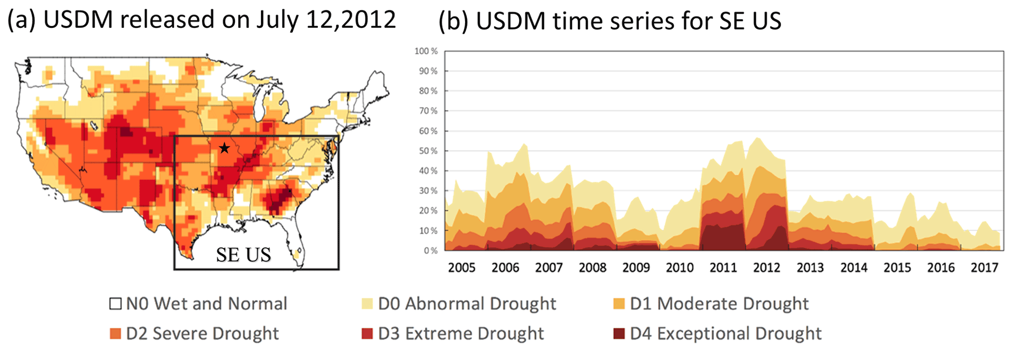
Figure 1(a) Drought distribution for the second week of July 2012 based on the USDM. The black star indicates the location of the MOFLUX site. (b) Time series of drought frequency in the study area (black box in Fig. 1a) for JJA from 2005 to 2017. The color-coded drought conditions are as follows: N0 (white) for wet and normal, D0 (light yellow) for abnormal drought, D1 (yellow) for moderate drought, D2 (orange) for severe drought, D3 (red) for extreme drought, and D4 (brown) for exceptional drought.
The USDM is a composite drought index based on six key physical indicators including the Palmer drought severity index (PDSI; Palmer, 1965), Climate Prediction Center (CPC) soil moisture model percentiles (Huang et al., 1996), United States Geological Survey (USGS) daily streamflow percentiles (https://waterwatch.usgs.gov/, last access: 20 October 2022), percent of normal precipitation (Willeke et al., 1994), standardized precipitation index (SPI; McKee et al., 1993), and remotely sensed satellite vegetation health index (Kogan, 1995). Opinions of local experts are also considered (Svoboda et al., 2002). The USDM website (https://droughtmonitor.unl.edu/, last access: 20 October 2022) provides weekly ArcGIS shapefiles of the polygons covering the whole US under five drought levels: D0 for abnormal drought, D1 for moderate drought, D2 for severe drought, D3 for extreme drought, and D4 for exceptional drought. We used the method of Chen et al. (2019) to rasterize and convert the USDM shapefiles to 0.5∘ × 0.5∘ gridded indices with −1 indicating non-drought (N0) and 0, 1, 2, 3, and 4 indicating D0, D1, D2, D3, and D4 drought, respectively. Figure 1a displays the spatial distribution of gridded USDM indices for the second week of July 2012, which clearly depicts the extent and severity of the infamous 2012 Great Plains drought (Hoerling et al., 2014). Figure 1b shows the weekly time series of USDM indices averaged over SE US (25–40∘ N, 75–100∘ W; black box in Fig. 1a) for the summer months (June–July–August, JJA) of 2005–2017, our study period. During this period, abnormal drought (D0) appeared every summer, while extreme and exceptional drought (D3–D4) were mainly concentrated in 2006–2008 and 2010–2012. This pattern is consistent with the long-term drought statistics from other drought indices such as the standardized precipitation–evapotranspiration index (SPEI) and PDSI (Svoboda et al., 2015).
2.2 OMI HCHO and NO2 product
We used the Ozone Monitoring Instrument (OMI) v003 Level 3 tropospheric formaldehyde (HCHO) column density (OMHCHOd), as described by Chance (2019). OMI was launched on NASA's Aura satellite in 2004 and has since provided daily global measurements of ozone (O3) and its precursors with a nadir spatial resolution of 24 × 13 km2. Since January 2009, OMI has been suffering from a major row anomaly. OMHCHOd data processing explored all Level 2 OMHCHO observations to filter out pixels with bad formaldehyde retrievals, high cloud fractions (>30 %), high solar zenith angle (SZA >70∘), and pixels affected by OMI's row anomaly (Chance, 2019). The spatial resolution is 0.1∘ × 0.1∘. Zhu et al. (2016) verified the OMHCHOd data using high-precision HCHO aircraft observations obtained during NASA SEAC4RS activities in SE US from August to September 2013. They showed that OMI retrievals have accurate spatial and temporal distribution but were biased low by 37 % relative to the aircraft. We corrected this underestimation by applying a uniform and constant factor of 1.5 to the OMHCHOd data, as also done by Shen et al. (2019) in their long-term analysis of OMI HCHO. Figure 2a presents the corrected OMHCHOd for the SE US averaged over JJA 2005–2017, where higher levels of HCHO are clearly seen over forested regions in Missouri, Georgia, Arkansas, and Texas. The OMHCHOd values shown hereafter are those with the correction factor applied. Although it is not known if the correction factor has temporal spatial variations during our study period, its application produced a good match between OMI and simulated HCHO columns under non-drought (N0) conditions (Fig. 2c). To examine the concurrent changes in nitrogen oxides (NOx = NO2 + NO) under drought conditions, we also used the Level 3 tropospheric column of NO2 from OMI during the same period (Krotkov et al., 2019).
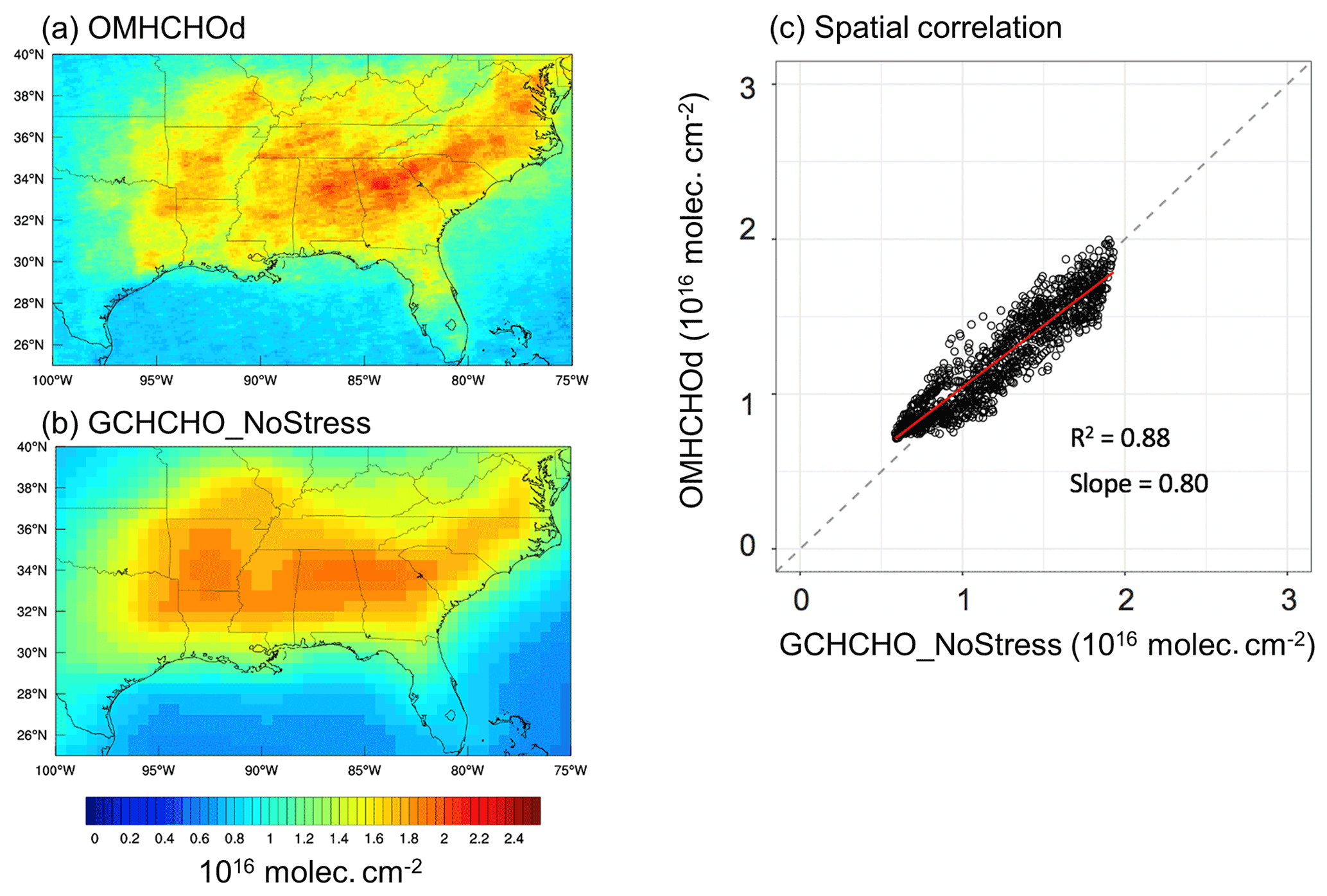
Figure 2Mean 2005–2017 HCHO columns for June–August over the SE US for (a) OMI observations (OMHCHOd) and (b) GEOS-Chem simulations (GCHCHO_NoStress). (c) Scatterplot of the spatial correlation between the two. The dashed line indicates the 1:1 agreement.
2.3 GEOS-Chem chemical transport model
We used the long-term simulation of the nested-grid GEOS-Chem global chemical transport model (version 12-02, http://www.geos-chem.org, last access: 21 October 2022) to obtain hourly results of modeled formaldehyde columns and isoprene emissions for North America during JJA 2005–2017. The simulation was driven by Version 2 of the Modern-Era Retrospective analysis for Research and Applications (MERRA-2) meteorological data from NASA's Global Modeling and Assimilation Office (GMAO) with a horizontal resolution of 0.5∘ × 0.625∘. Biogenic emissions were calculated using MEGAN2.1, which is the prevailing version of MEGAN implemented in most chemical and climate models. MEGAN2.1 has a soil dependence algorithm whose parameterization is based on the plant wilting point threshold and soil moisture (Guenther et al., 2017). However, this factor is disabled in GEOS-Chem, as in many other chemical transport models (CTMs), due to the unavailability of the required driving variables, such as wilting point and soil moisture, which cannot be simulated well in most models (Trugman et al., 2018). Thus, outputs from the standard GEOS-Chem simulations do not include drought effects on isoprene emissions, and these outputs are referred to as NoStress_GC. Anthropogenic emissions over North America were from the 2011 National Emissions Inventory (NEI2011, http://www.epa.gov/air-emissions-inventories, last access: 21 October 2022) for the United States, with historical scale factors applied to each simulated year. Open fire emissions were from GFED4 (Giglio et al., 2013) for 2005–2017.
To ensure a better match with the OMI overpass time, model HCHO outputs at 13:30 LT (local time) were sampled (GCHCHO_NoStress). Figure 2b shows GCHCHO_NoStress averaged over the same domain and period as OMHCHOd in Fig. 2a. The scatterplot in Fig. 2c shows a good spatial correlation between the two (R2=0.88). This correlation is consistent with other studies comparing GEOS-Chem and OMI HCHO columns in the SE US during non-drought periods (Kaiser et al., 2018).
2.4 Observations of ozone, organic aerosol, leaf area index, and isoprene flux
To evaluate how the drought stress factor changes the simulations of surface O3 and organic aerosol (OA), we adopted the gridded (1∘ × 1∘) hourly O3 observations created by Schnell et al. (2014) using the modified inverse distance weighting method. The dataset aggregates several networks of O3 measurements including the Air Quality System (AQS) and Clean Air Status and Trends Network (CASTNET) of the US Environmental Protection Agency (EPA) and the National Air Pollution Surveillance Program (NAPS) managed by Environment and Climate Change Canada (ECCC). Following the same method, we created a gridded organic aerosol (OA) dataset using the organic carbon (OC) observations from the Interagency Monitoring of Protected Visual Environments (IMPROVE) network. A factor of 2.1 was used to convert OC to OA, as suggested by other studies (Pye et al., 2017; Schroder et al., 2018). To examine the changes in the leaf area index (LAI) under drought conditions, the MODerate resolution Imaging Spectroradiometer (MODIS) Collection 5 LAI products reprocessed by Yuan et al. (2011) with a resolution of 0.25∘ × 0.25∘ were used. These three datasets were further remapped through bilinear interpolation to match the spatial resolution of the USDM. The isoprene flux measurements at the MOFLUX site during May–September 2012 were used to derive a site-based drought stress algorithm. The site is located in the Ozarks region of central Missouri (38.74∘ N, 92.20∘ W; black star in Fig. 1a). It is surrounded by a deciduous forest dominated by isoprene-emitting white and red oak species. The dataset has been widely used to investigate the response of isoprene emissions to droughts (Potosnak et al., 2014; Seco et al., 2015; Jiang et al., 2018; Opacka et al., 2022).
3.1 Changes in HCHO column densities with drought
To reveal drought responses of HCHO, we sampled weekly mean HCHO columns onto the gridded spatial and temporal locations of each USDM category and generated average HCHO distributions at each drought level over the SE US. The outputs are shown in Fig. 3a for OMI and in Fig. 3b for NoStress_GC. The processing of weekly mean HCHO data corresponds to the timing of the USDM: a whole week includes Wednesday of the previous week to Tuesday of the present week. There are 12 consecutive weeks from June to August in each year from 2005 to 2017, giving a total of 156 weeks of gridded HCHO data to be assigned to individual USDM categories by week and location. Figure 3d shows the number of weeks underlying the gridded averages of HCHO for each USDM category. As severe droughts are less frequent than mild droughts, some locations in the SE US did not experience D2–D4 droughts during the study period; hence, they are shown using white in Fig. 3.

Figure 3The mean spatial distributions of (a) OMI HCHO column density, (b) NoStress_GC HCHO column density, (c) NoStress_GC isoprene emissions, and (d) the number of weeks during JJA 2005–2017 in the SE US under different USDM drought levels (N0 and D0–D4).
OMI HCHO column density increases with increasing drought severity in almost all locations in the SE US (Fig. 3a). Relative to non-drought conditions (N0), the mean HCHO column from OMI is 6.7 %, 12.6 %, 16.5 %, 21.2 %, and 23.2 % higher under D0, D1, D2, D3, and D4 drought conditions over the entire SE US, respectively. These HCHO changes are statistically significant at a 95 % confident interval, indicating that the OMI HCHO products contain significant drought signals. The increasing rate of OMI HCHO with the USDM is not linear: it is faster under mild droughts (D0–D2) and flattens under more severe droughts (D2–D4). This is qualitatively consistent with the conceptualized model of the nonlinear response of isoprene emissions to drought that has been previously described (Potosnak et al., 2014).
Model HCHO column density also increases with increasing drought severity (Fig. 3b). GCHCHO_NoStress is 9.90 %, 15.1 %, 19.5 %, 21.8 %, and 29.1 % higher under D0, D1, D2, D3, and D4 drought than that of N0, respectively. These increases are 1.1–1.5 times those of OMI under all drought levels. The model comparison against OMI HCHO also changes with drought severity. GCHCHO_NoStress has a minimal bias (0.05 × 10¹⁶ molec. cm−2) under N0. As drought severity increases, the mean bias over the entire SE US increases to 0.10 × 10¹⁶, 0.09 × 10¹⁶, 0.11 × 10¹⁶, 0.08 × 10¹⁶, and 0.15 × 10¹⁶ molec. cm−2 under D0, D1, D2, D3, and D4 levels, respectively. The spatial correlation between OMI and NoStress_GC degrades with the USDM, with R2 being smaller than 0.65 under D0–D4 levels compared with the R2 of 0.70 under N0. Worsening model performance with increasing drought severity suggests that the model lacks a process that changes with drought. As isoprene accounts for more than 80 % of the contribution of non-methane VOCs to the HCHO column in the SE US (Palmer et al., 2003; Millet et al., 2006), the missing process is most likely drought-induced changes in isoprene emissions.
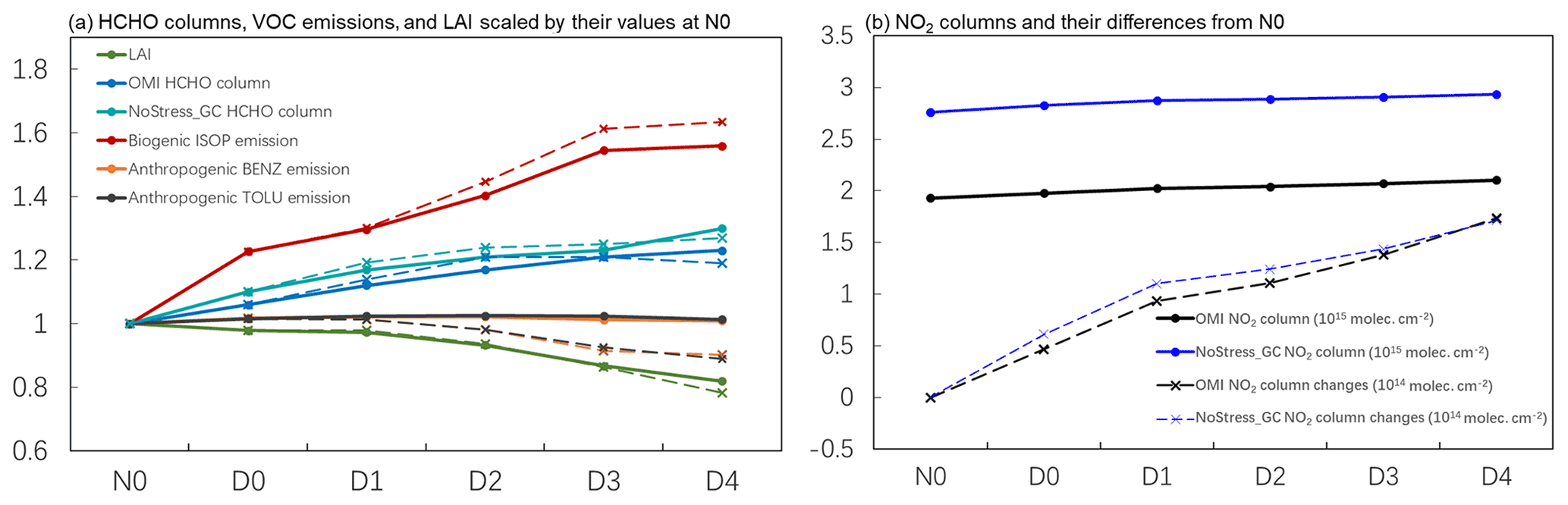
Figure 4(a) Relative changes in the regional-mean OMI HCHO column and NoStress_GC simulated HCHO column; isoprene, anthropogenic benzene, and anthropogenic toluene emissions; and MODIS leaf area index (LAI) under different drought levels in the SE US. All data are scaled to their respective values at N0. The dotted lines are the arithmetic mean of all grids, and the solid lines are the corrected mean excluding the missing area. (b) Regional-mean tropospheric NO2 columns from OMI and NoStress_GC (solid lines) as well as their respective changes from non-drought (N0) conditions (dashed lines). Note the different scales between the solid and dashed lines. The calculation is based on the grids with the presence of all USDM levels.
Figure 4a displays the relative changes in the regional mean HCHO column from OMI and NoStress_GC, emissions of isoprene and select anthropogenic VOCs from NoStress_GC, and the MODIS LAI as a function of the USDM indices, each scaled by its respective value at N0. The dotted line is the arithmetic mean of all available grids under each dryness category, and the solid line is the mean for those grids with valid data in all dryness categories (i.e., removing the white areas shown in Fig. 3). In both calculations, NoStress_GC overestimates the relative increase in HCHO under D0–D4 by 10 %–50 % compared with OMI. After correcting for areas with no data in D2–D4, isoprene emissions in NoStress_GC are 22.7 %, 29.6 %, 40.3 %, 54.5 %, and 56.0 % higher in D0, D1, D2, D3, and D4 than in N0, respectively. Note that the LAI is observed to decrease by 5 %–10 % per USDM level (Fig. 4a), which makes the predicted increase in isoprene emissions with drought severity even more remarkable. This is likely caused by the increasingly higher temperature under droughts, given the exponential relationship of isoprene emissions with temperatures in MEGAN (Guenther et al., 2006).
By comparison, the modeled increase in the HCHO column with drought is 12 %–25 %, which is more buffered than that of isoprene emissions. This is mainly caused by the loss of HCHO to photolysis, which is expected to increase under droughts with clearer skies (Wang et al., 2017; Naimark et al., 2021). In addition, HCHO formation also depends on the abundance of oxidants, such as hydroxyl radicals (OH) and NOx, that oxidize isoprene. High isoprene emissions can suppress OH under the low-NOx conditions that prevail in part of the SE US (Wells et al., 2020), leading to the buffered response in HCHO. Previous studies (Travis et al., 2016; Kaiser et al., 2018) have shown that the NEI2011 anthropogenic inventory in the model is biased high in the SE US, and a 60 % reduction in NOx emission has been suggested. By comparison with the OMI NO2 column, we found that NoStress_GC indeed overestimates NO2 columns by ∼ 42 % in the SE US (Fig. 4b), but the absolute bias in NO2 is nearly constant from N0 to D4 (solid lines in Fig. 4b). The NO2 column also shows an increasing trend from N0 to D4, although with a much smaller rate (less than 9 %) than HCHO. The model captures the relative change in the NO2 column with the USDM (dashed lines in Fig. 4b), despite the high bias due to the NEI2011 inventory, which indicates that the changes in natural sources of NOx (e.g., biomass burning and soil NOx) with droughts are well represented by NoStress_GC. To further examine the effect of the high bias of NOx on simulated HCHO, we conducted a sensitivity simulation that involved reducing the NEI2011 NOx emissions by 50 % over the SE US during JJA 2011–2013. Most of the SE US was experiencing drought conditions during the summertime of 2011–2012, whereas 2013 was a less drought-stricken year (Fig. 1). The sensitivity simulation resulted in a small reduction in the simulated HCHO column, and the change was nearly constant among the USDM levels (Fig. S1a–b), ranging from −0.04 × 10¹⁶ molec. cm−2 (2.6 %) to −0.05 × 10¹⁶ molec. cm−2 (3.5 %). This rules out the possibility that the high NOx bias in the model is the reason for the overestimation of HCHO under drought conditions. Given the suppression effect of isoprene on OH and the well-captured NO2 relative changes under drought conditions, the overestimation of HCHO columns by the model is unlikely to be caused by model chemistry and is more likely due to the overestimation of isoprene emissions under drought conditions.
While the oxidation of anthropogenic VOCs also produces HCHO, using benzene and toluene as indicator species, we found no change in anthropogenic VOC emissions with drought in the model (Fig. 4a). This insensitivity rules out anthropogenic VOCs as a key driver of the model overestimation of HCHO under drought conditions. If anything, we expect anthropogenic VOC emissions to increase during drought due to higher evaporative emissions driven by higher temperature and more fossil fuel consumption due to higher demand for space cooling. Wildfires are another important source that can lead to high HCHO levels, but their contributions to HCHO are more likely to be underpredicted in GEOS-Chem, partly due to insufficient hydrocarbon emissions and the underrepresented fire plume chemistry (Alvarado et al., 2020; Liao et al., 2021; Zhao et al., 2022). A deeper planetary boundary layer (PBL) is expected under drought conditions, primarily due to a larger sensible height flux released from dry soil (Miralles et al., 2014). Indeed, the MERRA-2 PBL height used in our simulation increases by 12.42 %, 17.79 %, 20.99 %, 26.21 %, and 29.52 % from D0 to D4 relative to the value of 1589 m at N0 in the SE US during the midday period (13:30 LT). Considering that the PBL heights in MERRA-2 agree well with observations with only an overall 200 m low bias (Guo et al., 2021), we do not expect mixing heights to be the main cause of the high bias of the HCHO column under drought conditions. To further quantify the effects of wildfires and the PBL on the changes in the HCHO column with drought, we conducted two additional sensitivity tests: (1) turning off the GFED4 wildfire emission inventory during JJA 2011–2013 and (2) keeping the PBL constant as in 2013 (normal year) during JJA 2011–2012 (drought years). The results in Fig. S1c–d show overall negligible changes in the HCHO column in the SE US, which verifies our abovementioned assumptions.
In summary, the model overestimates HCHO increases during drought compared with OMI. This overestimation is attributed to the model overestimation of isoprene emissions during drought. Thus, the drought stress effect on isoprene emissions is required in GEOS-Chem to resolve the discrepancy in HCHO responses to drought between OMI and the model.
3.2 Isoprene flux measurement
To further evaluate isoprene emissions in NoStress_GC, we compared the isoprene flux measurements at the MOFLUX site (Potosnak et al., 2014; Seco et al., 2015) with predicted isoprene emissions at the model grid that contains the site. At the time of writing, the MOFLUX site is the only long-term, canopy-level, biogenic isoprene flux measurement site in the Northern Hemisphere midlatitudes that sampled droughts. The site experienced multiple drought levels in the summer of 2012, which allows for model–observation comparison across different drought severities, as shown in Fig. 5. The abnormal dry conditions (D0) started in early June, developed into moderate drought (D1) in late June, worsened to severe drought (D2) and extreme drought (D3) in July–August, and bounced back to D2 in September (Fig. 5a). The model generally captures the daily variability in isoprene emissions with a statistically significant correlation coefficient (R) of 0.67, but its biases differ by USDM levels. The model underestimates isoprene flux from N0 (bias of −1.81 mg m−2 h−1) to D1 (bias of −2.89 mg m−2 h−1), has a minimal bias (−0.47 mg m−2 h−1) at D2, and changes to an overestimate at D3 (bias of 1.2 mg m−2 h−1) (Fig. 5b). While differences are expected when comparing a single-point flux measurement with the grid-mean model prediction, such differences most likely result in a systematic bias that should not relate to the temporal variability in drought. The fact that the model bias changes from being underpredicting to overpredicting as drought severity increases further confirms the importance of the lack of a drought suppression effect on isoprene emissions in the model during severe to exceptional droughts (D3 and D4). This is qualitatively consistent with that of the HCHO biases described above.
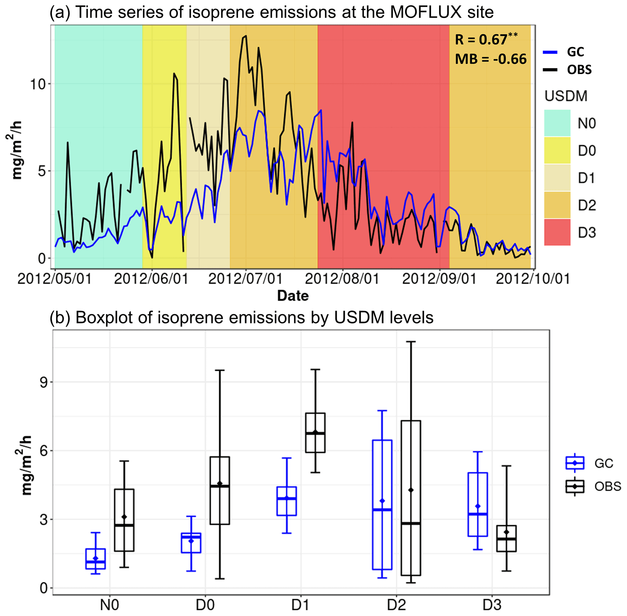
Figure 5(a) Comparison of daily time series of isoprene emissions observed at the MOFLUX site (OBS) and simulated by MEGAN2.1 in GEOS-Chem (GC). The background is color-coded according to the USDM drought severity. The R and MB values in the upper right-hand corner show the correlation coefficient and mean bias, respectively. (b) Boxplot of isoprene emissions separated by USDM drought levels. The upper and lower whiskers represent the 90 % and 10 % quantiles, respectively.
The MEGAN2.1 isoprene emission routines in GEOS-Chem use a simplified mechanistic representation of the major environmental factors controlling biogenic emissions (Guenther et al., 2012). In this representation the isoprene emission factor γ2.1 is the product of a canopy-related normalization factor (CFAC) multiplied by other factors representing light (γPAR), temperature (γT), leaf age (γAGE), LAI (γLAI), carbon dioxide (CO2) inhibition (), and soil moisture (γSM):
where γ0 is the product of the non-drought factors. Because of the lack of reliable soil moisture databases, γSM is always set to be one in GEOS-Chem, as in many other CTMs, which means no water stress term in the standard model configuration (i.e., NoStress_GC). Above, we show that NoStress_GC overestimates isoprene emissions and, consequently, HCHO column densities under drought conditions in the SE US. In this section, we describe the approach whereby observational constraints from the MOFLUX isoprene flux measurement and OMI HCHO were separately used to derive a drought stress factor γd that replaces γSM in Eq. (1) to simulate the response of isoprene emissions to drought in the MEGAN2.1 implementation of GEOS-Chem (hereafter referred to as GC/MEGAN2.1). The drought stress factor γd derived from the MOFLUX isoprene flux measurement is denoted as γd_MOFLUX and that from OMI HCHO is denoted as γd_OMI. Their corresponding simulations are referred to as MOFLUX_Stress_GC and OMI_Stress_GC, respectively. In both algorithms, the underlying assumption is that the GEOS-Chem model has no significant bias in predicting isoprene fluxes nor HCHO columns due to factors other than isoprene emissions under drought conditions. This assumption is reasonable because the GEOS-Chem model uses reanalysis meteorology, state-of-the-science isoprene oxidation schemes, time-specific anthropogenic emissions and fire emissions, and natural emissions calculated online using model meteorology, as described in Sect. 2.3. The discussion in Sect. 3.1 validated some aspects of the assumption, such as NOx emissions, wildfire emissions, and the PBL.
4.1 MOFLUX-based drought stress algorithm
The γd_MOFLUX was derived following Jiang et al. (2018) by implementing photosynthesis and water stress parameters with a formula of
where Vcmax is the maximum carboxylation rate by photosynthetic RuBisCO enzyme, and βt represents the water stress ranging from zero (fully stressed) to one (no stress). This simplified method intends to use the decreased photosynthetic enzyme activity to physiologically represent the variation in isoprene emissions under drought stress via dividing Vcmax by an empirical parameter α when the water stress is below a threshold.
As the default GEOS-Chem does not have these photosynthetic parameters, we adopted the ecophysiology module created by Lam et al. (2022) that is based on the photosynthesis calculation in the Joint UK Land Environmental Simulator (JULES; Best et al., 2011; Clark et al., 2011) as an online component in GEOS-Chem so that it simulates photosynthesis rate and bulk stomatal conductance dynamically and consistently with the underlying meteorology that drives GEOS-Chem. The outputs of Vcmax and βt from the ecophysiology module were passed to MEGAN2.1 in GEOS-Chem to parameterize the drought stress according to Eq. (2). In addition to GEOS-Chem meteorology, the ecophysiology module uses soil parameters from the Hadley Centre Global Environment Model, version, 2 Earth system model (HadGEM2-ES). In general, the implementation of the ecophysiology module much improved the simulated stomatal conductance and dry-deposition velocity relative to site observations on average for seasonal timescales, but the βt computed has not been calibrated to intermittent drought conditions. Instead of adopting the values of Vcmax and βt from Jiang et al. (2018), which were based on the Community Land Model, we need to determine the βt threshold and the α value specific to GEOS-Chem with the ecophysiology module of Lam et al. (2022). To calibrate βt, we first examined the statistical distribution of βt at the MOFLUX grid (Fig. S2) during May–September 2011 and 2012 when multiple USDM drought categories occurred. We then decided on a value of 0.3 as the threshold βt below which drought stress will be triggered in the model, as this value is greater than the 75 % quantile of all of the βt values from D0 to D3 and, thus, captures most of the drought conditions.
We note the observed isoprene flux at MOFLUX is consistently higher than predicted values during the non-drought period (e.g., N0 in Fig. 5a). This systematic bias is expected because we compare the single-point observations with grid-mean isoprene emission fluxes. To correct the systemic bias, we scaled down the model isoprene emissions at the MOFLUX grid by a factor of 1.42, which is the ratio of the average hourly isoprene fluxes between observations and simulations at the MOFLUX grid during non-drought conditions (βt>0.3). The factor of 1.42 was applied to downscale modeled isoprene fluxes at the MOFLUX grid during the entire time series, including drought conditions. The resulting time series are shown in Fig. 6a. Based on the downscaled model prediction, we derived that α=77 under drought conditions (βt<0.3), which minimized the mean bias under drought conditions between the modeled and observed isoprene fluxes in the MOFLUX grid.
Figure 6b shows the comparison of the hourly NoStress_GC and MOFLUX_Stress_GC isoprene emissions with observations in May–September 2012. The overall mean bias is reduced from 2.05 to 0.01 mg m−2 h−1 despite the fact that the stress factor is only applied to drought conditions. The correlation coefficient (R) and index of agreement (IOA) also increase from 0.77 to 0.85 and from 0.80 to 0.93, respectively. All of the changes in the comparison metrics indicate that the model simulations are improved considerably based on the single-point measurement.
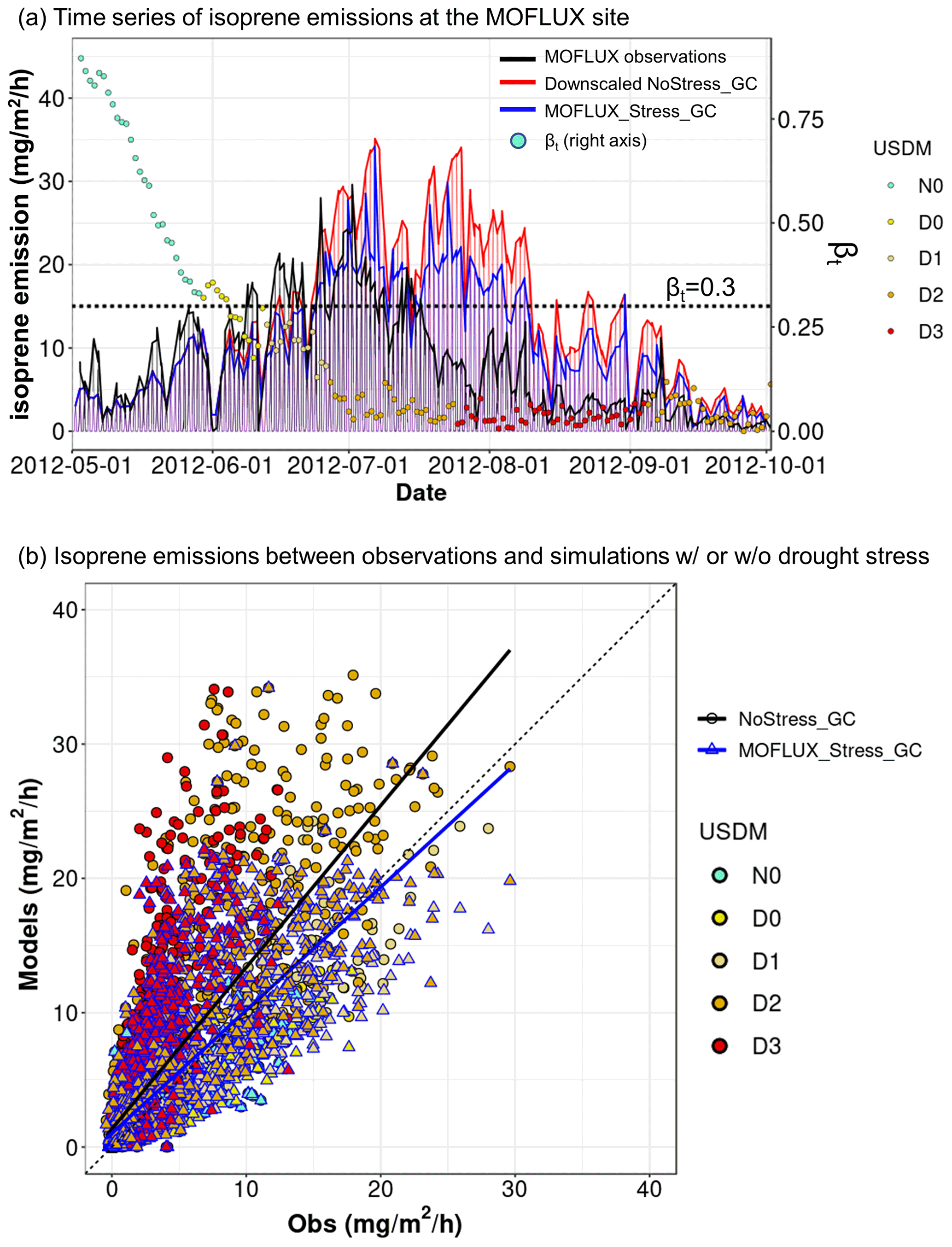
Figure 6(a) Hourly time series of isoprene emissions at the MOFLUX site from observations (black line) and simulations with (MOFLUX_Stress_GC; blue line) and without (NoStress_GC; red line; after downscaling) drought stress. The dots, color-coded by USDM levels, represent the daily values of βt (right axis). The dashed line indicates the threshold of 0.3. (b) Comparison of isoprene emissions between observations (Obs) and simulations with (MOFLUX_Stress_GC; blue-bordered triangle) and without (NoStress_GC; black-bordered circle) drought stress.
4.2 OMI-based drought stress algorithm
Isoprene emission increases exponentially at temperatures below ∼ 310 K (Guenther et al., 2006) in the absence of other stress factors such as drought. Indeed, an exponential relationship between biogenic isoprene emission per unit LAI and temperature is predicted by MEGAN2.1 at all USDM levels (Fig. S3). However, the predicted temperature sensitivity is found to increase substantially with drought severity with no sign of plateauing or slowing down, even under the most severe drought conditions when MOFLUX measurements measured a decrease in isoprene emissions (see Fig. 5). Similarly, we found that NoStress_GC overestimates HCHO sensitivities to high temperatures (>300 K) under drought conditions (D0–D4) (Fig. 7), but no such overestimation is seen under non-drought (N0) or low-temperature conditions during drought (<300 K). This indicates that the impact of drought stress on isoprene emissions is likely via suppression of the dependence of emissions on temperatures during drought. Leaf-level measurements conducted during the 2012 drought at the MOFLUX site provide independent evidence of drought suppression of the isoprene response to increasing temperature for less drought-resilient tree species (Geron et al., 2016). Taking advantage of these empirical observations, we derived the OMI-based drought stress algorithm by minimizing the differences in HCHO column sensitivities to temperatures between OMI and GEOS-Chem under drought conditions, as shown in Fig. 7. When calculating the relationships between HCHO column densities and temperatures, we first scaled the HCHO column by the LAI on a grid-by-grid basis to account for the regional differences in isoprene emissions due to different vegetation coverage as well as the effect of LAI changes with drought (see Fig. 4). Each point in Fig. 7 represents the mean ratio, denoted as Ω, within each 1 K temperature interval. We used exponential functions () to separately fit the temperature (T) dependence of the ratio (Ω) for different drought levels (Fig. 7) for both the model and OMI. The resulting formulas are listed in Table 1, and the R2 of most fitting lines is greater than 0.9.
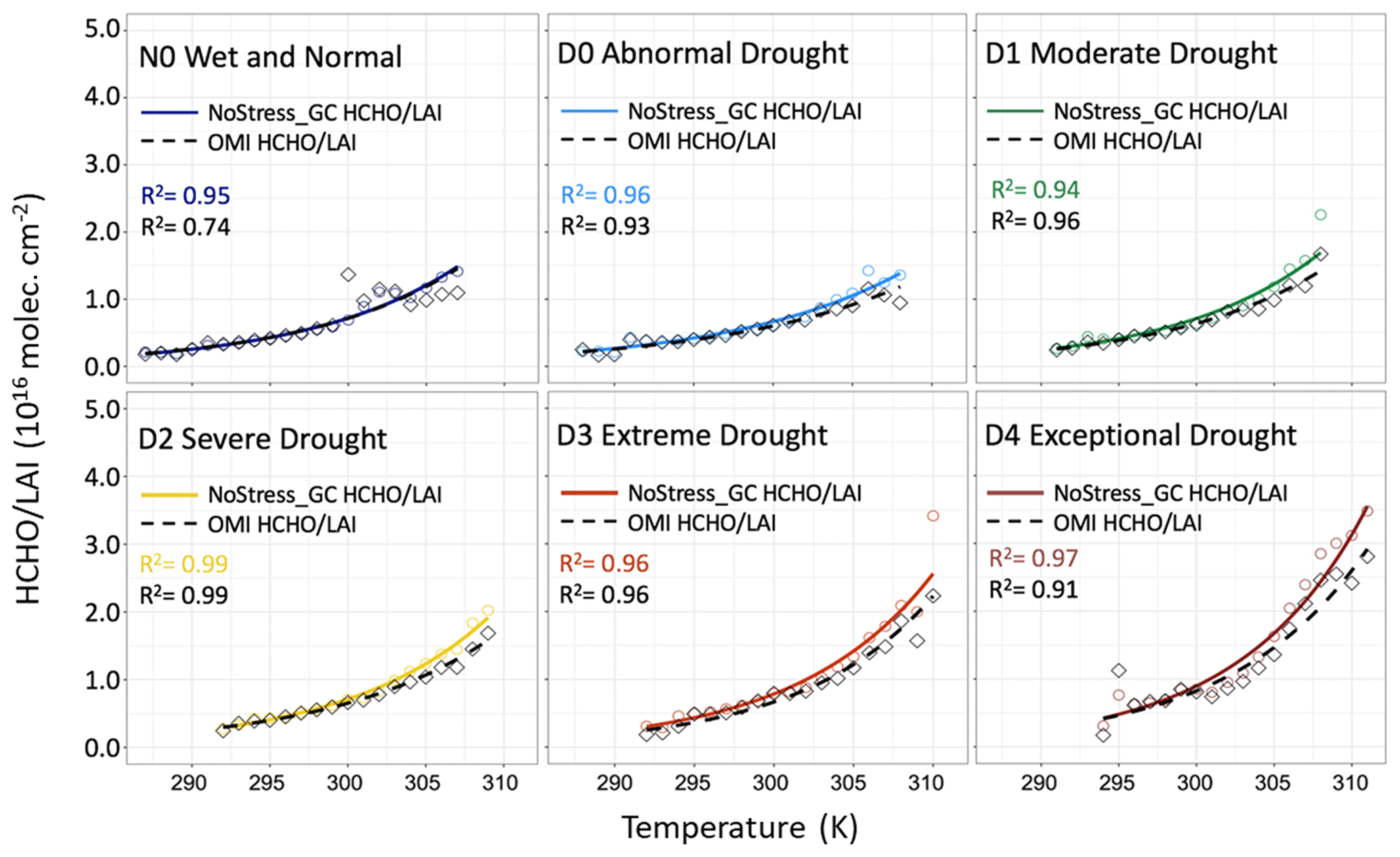
Figure 7Response of the ratio (1016 molec. cm−2) to temperature (K) for different drought levels averaged over JJA 2005–2017. The colored solid line is the modeled NoStress_GC ratio, and the black dashed line is the observed ratio from OMI. The exponentially fitted formulas and the resulting coefficient of determination (R2) are labeled in each subplot.
Table 1Fitted exponential formulas of the NoStress_GC and the OMI ratios (Ω, 1016 molec. cm−2) to surface air temperature (T, K) as well as the fitted value of the ratio at 290, 300, and 310 K.
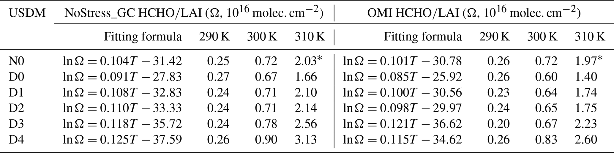
* An asterisk indicates that the temperature does not reach this value in the actual data and is an extrapolated value.
As the fitting equations suggest, both the NoStress_GC and OMI ratios increase with temperature under all conditions, but the former shows a higher sensitivity to temperature under drought conditions. This can clearly be seen from the higher ratios of NoStress_GC (ΩGC; solid lines) than those of OMI (ΩOMI; dashed lines), especially when the temperature is greater than 300 K under D0–D4. To better explain this, we also calculated the fitted value of at three temperatures of 290, 300, and 310 K, as shown in Table 1. As it is difficult for the N0 condition to reach a temperature of 310 K, the values were extrapolated and are marked with an asterisk in the table. The results show that the model overestimates the temperature dependence at all drought levels. At 290 K, all biases between ΩOMI and ΩGC are less than 0.05 × 10¹⁶ molec. cm−2. At 310 K, the bias between the two is 0.06 × 10¹⁶ molec. cm−2 (3.0 %) at N0 but increases by more than a factor of 4 to 0.26 × 10¹⁶ molec. cm−2 (18.6 %), 0.36 × 10¹⁶ molec. cm−2 (20.7 %), 0.39 × 10¹⁶ molec. cm−2 (22.3 %), 0.33 × 10¹⁶ molec. cm−2 (14.8 %), and 0.53 × 10¹⁶ molec. cm−2 (20.4 %) for the D0, D1, D2, D3, and D4 drought levels, respectively. As isoprene emission is a fixed function of temperature in MEGAN2.1, the overdependence of the HCHO column on temperature is caused by the previous 2 weeks' temperatures being higher under drought conditions, which leads to a higher value of γT, reflecting the temperature “memory” effects on isoprene emissions (Fig. S4). Based on the fitted formulas in Table 1, the ratio between under each level from D0 to D4 can be derived as follows:
where kOMI (kGC) and bOMI (bGC) represent the respective slopes and interpolations of the formulas in Table 1 for the OMI (GC) HCHO column, T is surface temperature, and e is the exponential constant. By averaging the values of kOMI–kGC and bOMI–bGC from D0 to D4, we can obtain
where βt<0.6 represents the 75 % quantile of the βt values from D0 to D4 for the whole SE US study region in JJA 2005–2017 (Fig. S2).
Thus, the formula for γd_OMI is
Note that the threshold of βt in Eq. (5) is different from the value used by γd_MOFLUX because all of the SE US grids were considered when deriving βt for γd_OMI. Another difference is that the factor is activated only if the temperature is higher than 300 K when significant biases between ΩOMI and ΩGC are found (Fig. 7).
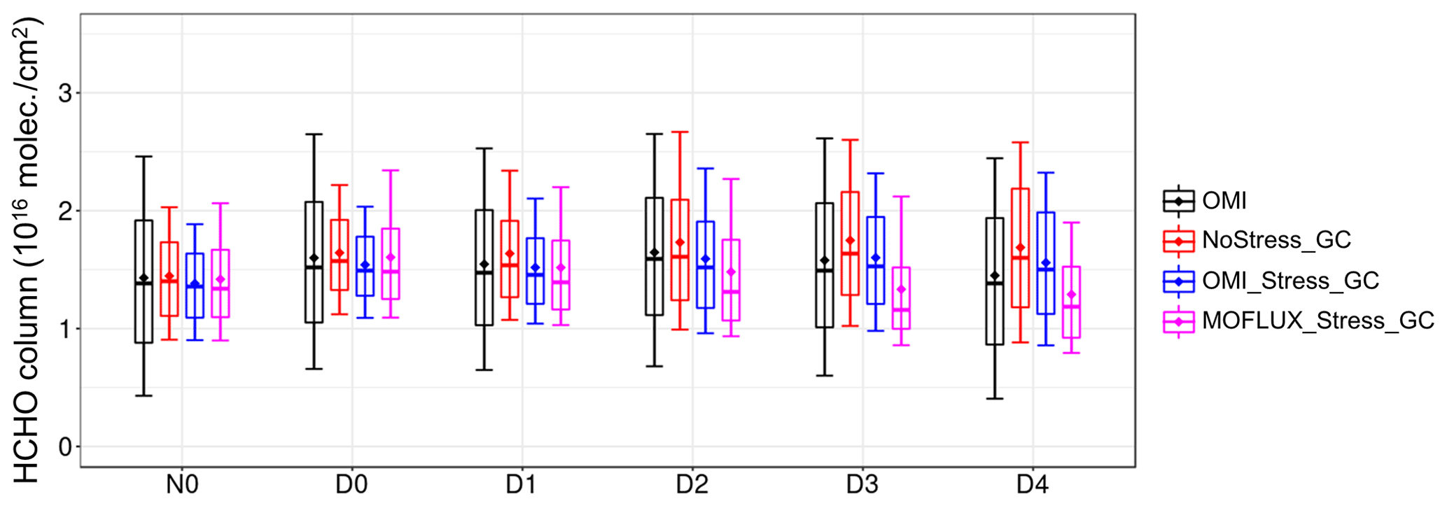
Figure 8Boxplot of HCHO column statistical distributions for OMI observations (black) and different GEOS-Chem simulations: without drought stress (NoStress_GC; red) and with drought stress factors derived from MOFLUX observations (MOFLUX_Stress_GC; blue) and from OMI HCHO constraints (OMI_Stress_GC; pink).
Figure 8 compares the statistical distributions of HCHO column densities from OMI, NoStress_GC, MOFLUX_Stress_GC, and OMI_Stress_GC during May–September 2012 over the SE US. Compared with OMI, NoStress_GC simulation has a mean high bias of 0.02 × 10¹⁶–0.24 × 10¹⁶ molec. cm−2 during D0–D4. The γd_OMI algorithm reduces the high bias to −0.05 × 10¹⁶–0.11 × 10¹⁶ molec. cm−2. By contrast, the γd_MOFLUX algorithm reduces the HCHO simulations too much over the SE US and causes an overall underestimation of 0.02 × 10¹⁶–0.25 × 10¹⁶ molec. cm−2. The γd_MOFLUX algorithm also narrows the statistical distribution of HCHO, as indicated by the smaller boxes and shorter whiskers compared to OMI. This suggests that the γd_MOFLUX algorithm based on the single-site observations is incapable of representing the drought stress over the SE US, possibly because the MOFLUX site has thin soil layers and, thus, is vulnerable to water stress (Opacka et al., 2022). Therefore, the isoprene emissions measured here are more sensitive to droughts, and the same extent of drought stress is likely too strong to be applied to other regions in the SE US. As a result, the γd_OMI algorithm is used in the next section to further evaluate how this algorithm would change the responses of atmospheric compositions to droughts.
In this section, we evaluated the changes in biogenic isoprene emissions and HCHO column densities by running a long-term (JJA, 2005–2017) simulation, after adding the OMI-based drought stress factor for isoprene emissions γd_OMI in GEOS-Chem. As isoprene is an important precursor for the formation of tropospheric O3 and OA, maximum daily 8 h average (MDA8) O3 as well as OA changes were also examined. We used the complexSOA mechanism in GEOS-Chem (Pye et al., 2010; Marais et al., 2016) which includes more detailed pathways of isoprene to secondary organic aerosols such as aqueous-phase reactive uptake and the formation of organonitrates.
Figure 9 shows the changes in biogenic isoprene emissions resulting from adding γd_OMI drought stress in GEOS-Chem. Here, we expanded the maps to the entire contiguous US to examine whether the drought stress algorithm can impose large changes on other US regions, although such changes need to be interpreted with caution. The numbers in each panel in Fig. 9 indicate the mean isoprene emissions for NoStress_GC and the mean differences (MD) relative to OMI_Stress_GC over the SE US. As expected, the biggest decrease in isoprene emissions is found in the SE US with the regional-mean emissions reduced by 0.17 × 10⁻¹⁰ kg m−2 s−1 (8.60 %), 0.35 × 10⁻¹⁰ kg m−2 s−1 (14.24 %), 0.43 × 10⁻¹⁰ kg m−2 s−1 (16.57 %), 0.49 × 10⁻¹⁰ kg m−2 s−1 (17.49 %), 0.58 × 10⁻¹⁰ kg m−2 s−1 (18.66 %), and 0.65 × 10⁻¹⁰ kg m−2 s−1 (20.74 %) for N0, D0, D1, D2, D3, and D4, respectively (Fig. 9c). Despite lowering emissions relative to NoStress_GC, OMI_Stress_GC simulates an increase in isoprene emissions under drought conditions compared with non-drought conditions in the SE US; the respective increases are 0.28 × 10⁻¹⁰ kg m−2 s−1 (15.20 %), 0.34 × 10⁻¹⁰ kg m−2 s−1 (18.40 %), 0.49 × 10⁻¹⁰ kg m−2 s−1 (26.47 %), 0.69 × 10⁻¹⁰ kg m−2 s−1 (37.46 %), and 0.65 × 10⁻¹⁰ kg m−2 s−1 (35.23 %) for D0, D1, D2, D3, and D4 relative to N0 (Fig. 9c). This increase results from the top-down constraints by the corresponding changes in OMI HCHO column densities with the USDM and, consequently, exhibits the behavior of nonuniform increases with drought severity (e.g., peak increase of 37.5 % at D3 followed by a ∼ 2 % reduction at D4), which is consistent with the MOFLUX flux measurements.
For other regions, such as California and Minnesota, biogenic isoprene emissions decreased slightly (by less than 0.5 × 10¹⁰ kg m−2 s−1). The smaller effect of the drought stress factor imposed on regions other than the SE US is understandable because of the lower isoprene emissions.
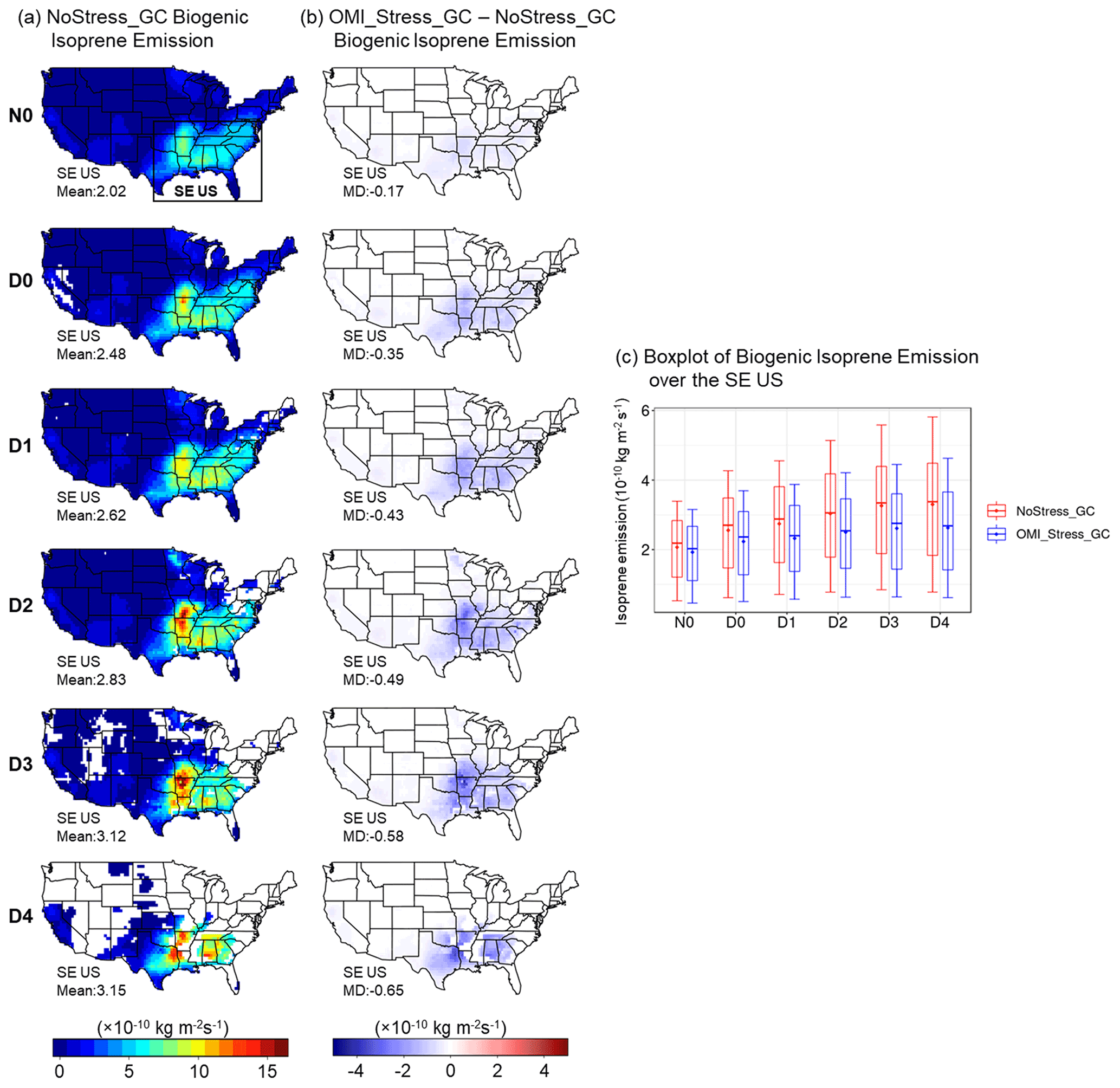
Figure 9Simulated biogenic isoprene emissions during JJA 2005–2017 by USDM dryness category for NoStress_GC (a) and OMI_Stress_GC minus NoStress_GC (b) as well as the statistical distributions of the SE US isoprene emissions between the two simulations (c). Numbers in the bottom left-hand corner of panel (a) indicate the SE US (black box) regional mean of biogenic isoprene emissions for NoStress_GC, whereas they indicate the mean difference (MD) between OMI_Stress_GC and NoStress_GC in panel (b).
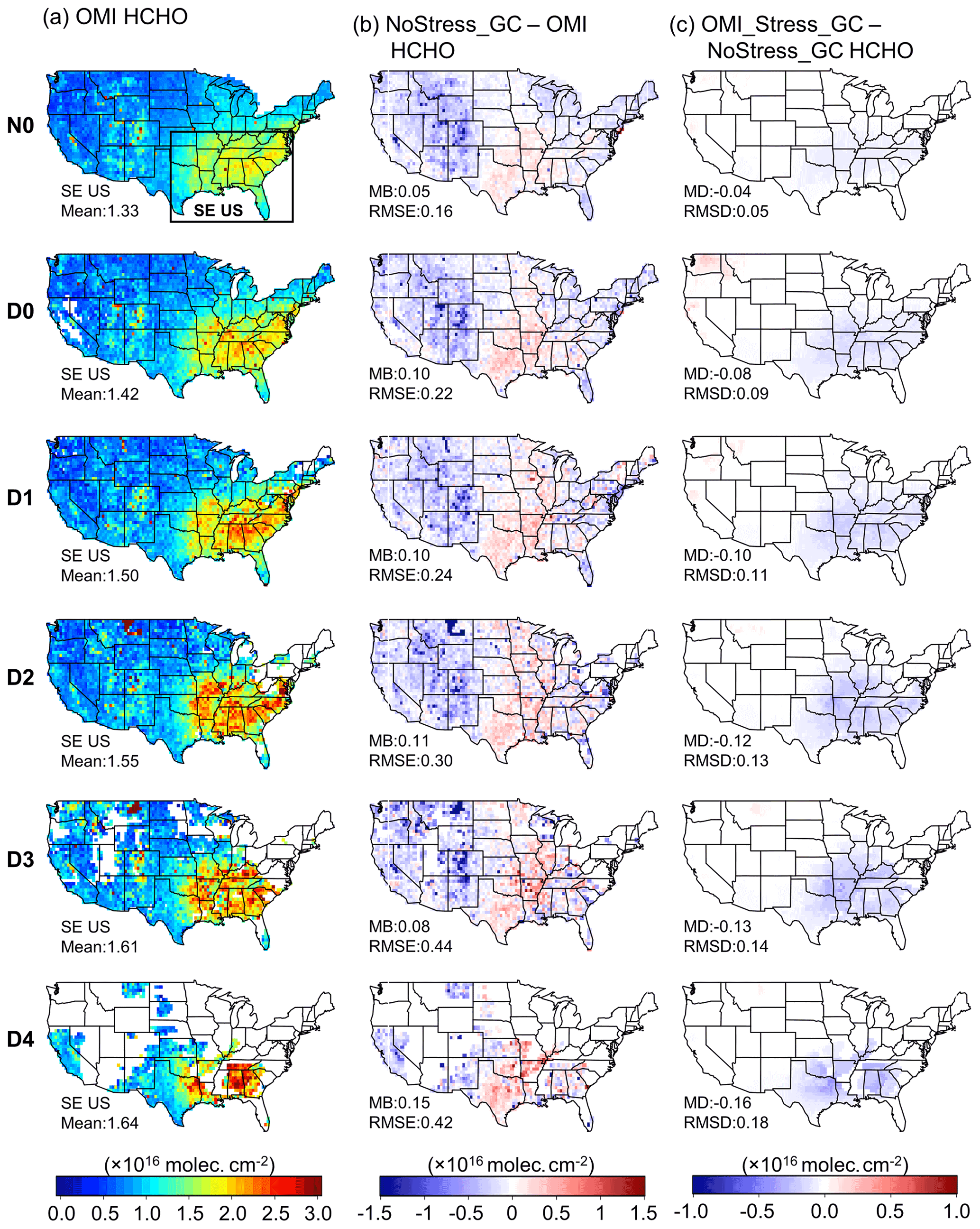
Figure 10Mean HCHO column densities during JJA 2005–2017 by USDM dryness category for OMI (a), NoStress_GC minus OMI (b), and OMI_Stress_GC minus NoStress_GC (c). Numbers in the bottom left-hand corner of panel (a) indicate the SE US (black box) regional mean of OMI HCHO column; numbers in the bottom left-hand corner of panel (b) indicate the mean bias (MB) and root-mean-square error (RMSE) in HCHO column densities between NoStress_GC and OMI; and numbers in the bottom left-hand corner of panel (c) indicate the mean difference (MD) and root-mean-square deviation (RMSD) between OMI_Stress_GC and NoStress_GC. The MD and RMSD are calculated in the same way as the MB and RMSE; however, the different names are used to distinguish between model–model comparison and model–observation comparison, respectively.
The changes in the HCHO column are shown in Fig. 10. Different from the overestimation in the SE US, NoStress_GC underestimates HCHO column densities in the western US compared with OMI (Fig. 10b). This negative bias should be interpreted with care because the scaling factor of 1.5 (see Sect. 2.2) is derived over the SE US and may not hold in other regions. For the SE US overall, the drought stress factor reduces modeled HCHO columns by 0.08 × 10¹⁶ molec. cm−2 (5.43 %), 0.10 × 10¹⁶ molec. cm−2 (6.46 %), 0.12 × 10¹⁶ molec. cm−2 (7.22 %), 0.13 × 10¹⁶ molec. cm−2 (7.62 %), and 0.16 × 10¹⁶ molec. cm−2 (8.91 %) under D0, D1, D2, D3, and D4, respectively, relative to NoStress_GC (Fig. 10c). This leads to better agreement with OMI, as OMI_Stress_GC has a near-zero MB under D0–D4 (Fig. S5; MB = −0.05 × 10¹⁶–0.02 × 10¹⁶ molec. cm−2). The RMSE is also reduced by 3 %–13 % relative to the NoStress_GC simulation compared with observations. The changes in both metrics indicate that the drought algorithm considerably improves the model performance with respect to capturing the biogenic isoprene response to drought, as evidenced by the HCHO column. Similar to the changes in biogenic isoprene emissions, the OMI_Stress_GC only slightly decreases HCHO column densities (<5 %) compared with the NoStress_GC simulation in other US regions.
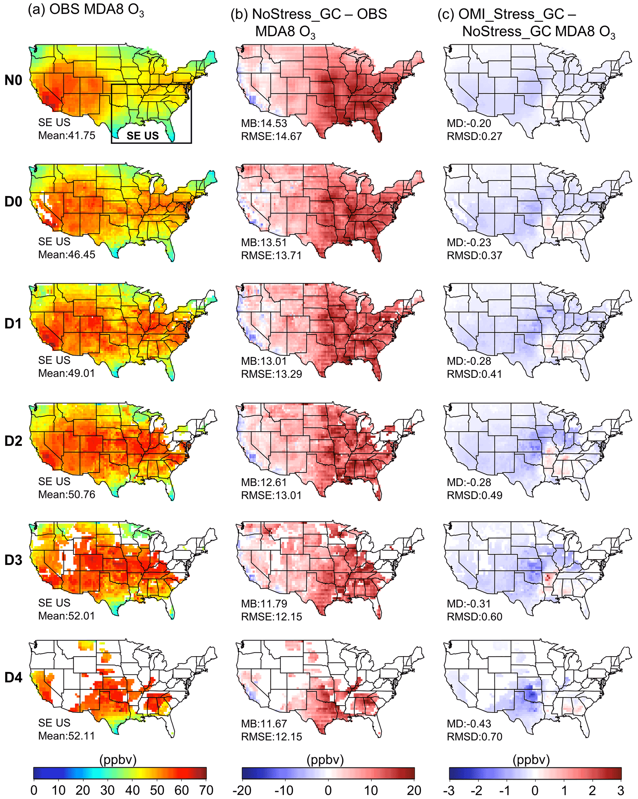
Figure 11Same as Fig. 10 but for surface maximum daily 8 h average (MDA8) O3.
Figure 11a displays the observed MDA8 O3 changes with the USDM. Similar to the changes in the HCHO column with USDM levels, O3 in the SE US exhibits a gradual increase, relative to the mean of 41.74 ppbv at N0, of 4.70 ppbv, 7.26 ppbv, 9.01 ppbv, 10.26 ppb, and 10.36 ppbv for D0, D1, D2, D3, and D4, respectively. This is consistent with our previous study (Li et al., 2022; Lei et al., 2022) that investigated O3 changes with drought severity in more detail. The NoStress_GC simulation has a high bias in MDA8 O3 across all USDM categories (Fig. 11b). High positive bias is a common issue for O3 simulations at the surface in CTMs, which is a research question and can be attributed to the uncertainties in various processes, such as NOx emissions, isoprene oxidation pathways, O3 dry-deposition velocity, and boundary layer dynamics (Fiore et al., 2005; Lin et al., 2008; Squire et al., 2015; Travis et al., 2016; Travis and Jacob, 2019). Despite the systematic high bias, NoStress_GC captures the increasing trend of MDA8 O3 with increasing dryness but with a respectively smaller increment (relative to N0) of 3.62, 5.67, 7.01, 7.41, and 7.41 ppbv for D0, D1, D2, D3, and D4. This discrepancy between NoStress_GC and observations can also be inferred from the fact that the MB between the model and observations decreases from 14.53 ppbv at N0 to 11.67 ppbv at D4 (Fig. 11b). Figure 11c shows the difference in MDA8 O3 between OMI_Stress_GC and NoStress_GC. In the SE US, where isoprene emissions are the highest and decrease the most due to the drought stress algorithm, OMI_Stress_GC shows a small increase in MDA8 O3 of less than 1 ppbv. This increase in O3 can be explained by an increase in OH resulting from decreasing isoprene emissions under low-NOx conditions in the SE US (Wells et al., 2020). For the SE US study domain as a whole, the change in MDA8 O3 was negligible but negative (regional mean of −0.5 ppbv). Although the drought factor does not reduce the overall high bias, it makes the model more consistent with the observed increment in MDA8 O3 for the subregion with increased O3 (e.g., 32–35∘ N, 90–94∘ W) as drought severity increases. As NOx has a high positive bias from the NEI2011 inventory (Fig. 4), the improvement in MDA8 in these regions is likely to be underestimated. Over northeastern Texas, Oklahoma, and Kansas, where isoprene emission is also reduced by the drought algorithm, although from a much lower emission base compared with other SE US areas, OMI_Stress_GC simulates 1–3 ppbv lower MDA8 O3 under drought conditions (D0–D4), leading to better agreement with observations. For regions with lower isoprene and higher NOx concentrations, O3 formation is more sensitive to the changes in isoprene, which explains the reduction in MDA8 O3 caused by the drought stress factor.
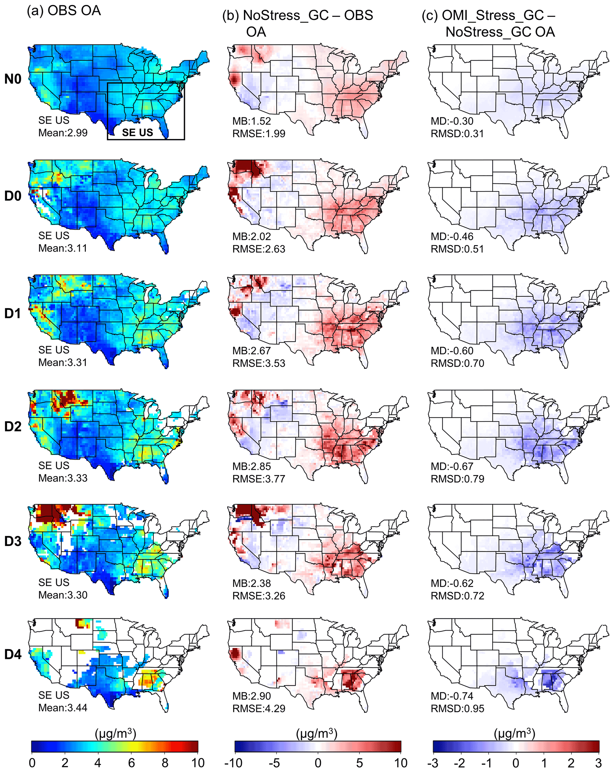
Figure 12Same as Fig. 10 but for organic aerosol (OA).
The changes in OA with the USDM are shown in Fig. 12. Observed OA in the SE US shows an average increase (relative to N0) of 0.12, 0.32, 0.34, 0.31, and 0.45 µg m−3 for D0, D1, D2, D3, and D4, respectively. The extremely high values over the northwestern states (e.g., Washington and Montana) are likely associated with higher wildfire emissions under drought conditions (Wang et al., 2017). The NoStress_GC simulation considerably overestimates OA in the SE US with an MB of 1.52 µg m−3 (50.83 %) at N0, and the overestimation becomes even higher (2.02–2.90 µg m−3, 64.95 %–85.58 %) at D0–D4 (Fig. 12b), thereby causing an overprediction of the drought–OA relationship. Zheng et al. (2020) reported a similar level of overestimation and attributed this to the overdependence of isoprene-derived secondary organic aerosol (SOA) on sulfate. As isoprene is one of the dominant sources of OA in the SE US (Xu et al., 2015; Budisulistiorini et al., 2016), our analysis suggests that the model overestimation of isoprene emissions under drought conditions is another reason for this high OA bias in the SE US. Indeed, the drought stress factor greatly improves the OA simulation by reducing the MB by 0.30 µg m−3 (6.60 %), 0.46 µg m−3 (8.98 %) 0.60 µg m−3 (10.07 %), 0.67 µg m−3 (10.85 %), 0.62 µg m−3 (10.88 %), 0.74 µg m−3 (11.71 %) for N0, D0, D1, D2, D3, and D4, respectively, over the SE US (relative to NoStress_GC) and, thus, lowering the MB to be within 1.22–2.18 µg m−3 (40.82 %–65.52 %; Fig. S5) compared with observations. We also examine the change in three major SOA components in Fig. S6. Anthropogenic SOA (ASOA) barely changes, whereas isoprene SOA (ISOA) decreases the most (as expected because the drought stress factor is applied to isoprene emissions only). Interestingly, terpene SOA (TSOA) also shows a slight decrease, suggesting positive feedback between ISOA and TSOA.
In summary, the OMI-based drought stress factor shows good performance with respect to correcting the overestimation of biogenic isoprene in default GEOS-Chem simulations under drought conditions. The drought stress factor was constrained by the observed exponential fitting between the HCHO / LAI ratio and temperature, not by observed HCHO columns directly. It nearly eliminates the high HCHO bias compared with OMI observations in the SE US under drought conditions, which consequently improves the simulation of OA. MDA8 O3 slightly increases in the areas with high isoprene emissions, leading to no improvement in the model bias but better agreement with the observed O3 increment with drought severity. Places with lower isoprene emissions show an MDA8 O3 reduction of 1–3 ppbv, indicating the region-specific O3 responses to the changes in isoprene due to the nonlinearity of O3 chemistry.
Using the long-term (JJA, 2005–2017) weekly USDM drought index and OMI HCHO column data over the SE US, we revealed a step-increase pattern in HCHO by 6.7 %, 12.6 %, 16.5 %, 21.2 %, and 23.2 % for D0, D1, D2, D3, and D4 relative to non-drought conditions (N0), respectively, which indicates the increasingly higher isoprene emissions with drought on a regional scale, although the rate of increase decreases under severe drought conditions. Compared with OMI observations, the GEOS-Chem simulated HCHO column density exhibits a similar pattern, but the changes are 1.1–1.5 times higher with a respective increase of 9.90 %, 15.1 %, 19.5 %, 21.8 %, and 29.1 % for D0, D1, D2, D3, and D4. As there are no big changes in anthropogenic VOCs under drought conditions, biogenic isoprene emissions are the key drivers for the increase in HCHO, and a drought stress factor is missing in the MEGAN2.1 biogenic inventory in the default GEOS-Chem simulations, causing the overestimation of the HCHO changes in response to droughts.
The MOFLUX site provides the only long-term ground-based isoprene flux observations covering multiple drought severities. We developed a drought stress algorithm based on the MOFLUX site following Jiang et al. (2018), and the algorithm improves the HCHO simulation at the MOFLUX grid while underestimating HCHO after all of the SE US grids are included. By comparison, the OMI-based drought stress algorithm derived from the different HCHO-temperature sensitivities between OMI and GEOS-Chem can reflect better spatial coverage and nearly removes the positive bias between OMI and the default simulations seen from a test simulation in May–September 2012 over the SE US.
The long-term simulation with the OMI-based drought stress factor can significantly reduce the biogenic isoprene emissions by 0.35 × 10⁻¹⁰ kg m−2 s−1 (14.24 %), 0.43 × 10⁻¹⁰ kg m−2 s−1 (16.57 %), 0.49 × 10⁻¹⁰ kg m−2 s−1 (17.49 %), 0.58 × 10⁻¹⁰ kg m−2 s−1 (18.66 %) and 0.65 × 10⁻¹⁰ kg m−2 s−1 (20.74 %) for D0, D1, D2, D3, and D4, respectively, which consequently leads to better agreement between OMI and the simulated HCHO column. Despite lowering emissions relative to the no-stress simulation, OMI_Stress_GC simulates a nonuniform trend of increasing isoprene emissions with drought severity that is consistent with OMI HCHO and MOFLUX. Relative to N0, the simulated increase in isoprene emissions is 15 %–18 % under D0–D1; this then increases to 26 % at D2, peaks at 37 % at D3, and is followed by a slight decrease to 35 % at D4.
The observed MDA8 O3 and OA over the SE US show a similar increase pattern with HCHO. The OMI-based drought stress algorithm also helps reduce the mean bias of OA by 0.30 µg m−3 (6.60 %), 0.46 µg m−3 (8.98 %) 0.60 µg m−3 (10.07 %), 0.67 µg m−3 (10.85 %), 0.62 µg m−3 (10.88 %), 0.74 µg m−3 (11.71 %) for N0, D0, D1, D2, D3, and D4, respectively, over the SE US compared with the high positive bias of more than 2.02 µg m−3 (50.83 %) without the drought stress. By contrast, the MDA8 O3 response to the reduced biogenic isoprene caused by the drought stress factor presents a spatial disparity due to the nonlinear O3 chemistry. Places with high isoprene emissions show an increase in the MDA8 O3 of less than 1 ppbv, which slightly improves the simulated drought–O3 relationship. For the regions with low isoprene emissions in the SE US, the drought stress factor reduces the MDA8 O3 by 1–3 ppbv.
This study reveals an increasingly higher level of biogenic isoprene under drought conditions over the regions with high vegetation coverage. As drought is predicted to become more frequent in a warming climate (Cook et al., 2018), it is essential to update current biogenic emission inventories by adding a drought stress factor and to improve the constraints of isoprene chemistry in the climate chemistry models in order to have a better projection of air quality in the future. We demonstrate the feasibility of applying satellite data to the development of drought stress algorithms when ground-based measurements are limited. Our attempt here is a top-down approach, and it used temperature as the only parameter to adjust isoprene emissions under drought conditions. The water stress threshold in our algorithm is used only as a triggering parameter; that is, it is used to determine whether a grid is experiencing drought or not and, thus, can be replaced with other drought-identifying approaches. One issue with our approach is the type of temperature data to be used in the algorithm. Ideally, it should be leaf temperature, as this is what regulates stomata at the process level. However, leaf temperature is not readily available from meteorological fields that drive CTMs. MEGAN uses 2 m air temperature to parameterize isoprene emissions; thus, our algorithm uses the same temperature. More biogenic emission flux observations covering different vegetation types and drought severities will be helpful to better depict the relationships between biogenic VOCs and drought stress.
The GEOS-Chem model is publicly available at https://doi.org/10.5281/zenodo.2572887 (The International GEOS-Chem User Community, 2019). The USDM shapefiles can be download from https://droughtmonitor.unl.edu/DmData/GISData.aspx (Svoboda et al., 2002). The LAI can be obtained from http://geoschemdata.wustl.edu/ExtData/HEMCO/Yuan_XLAI/v2021-06/ (Yuan et al., 2011). Ozone and organic carbon observational data can be downloaded from https://aqs.epa.gov/aqsweb/documents/data_mart_welcome.html (Schnell et al., 2014). Observational isoprene measurements at MOFLUX are sourced from Potosnak et al. (2014) and Seco et al. (2015) and are available upon request from co-author Alex Guenther. OMI Satellite HCHO and NO2 columns are publicly available from https://doi.org/10.5067/Aura/OMI/DATA3010 (Chance, 2019) and https://doi.org/10.5067/Aura/OMI/DATA3007 (Krotkov et al., 2019), respectively.
The supplement related to this article is available online at: https://doi.org/10.5194/acp-22-14189-2022-supplement.
YW conceived the research idea. NL and WL conducted the model simulation and data analysis. JCYL and APKT created the ecophysiology module. AG, MJP, and RS provided the field observations. All authors contributed to the interpretation of the results and the preparation of the manuscript.
The contact author has declared that none of the authors has any competing interests.
Publisher’s note: Copernicus Publications remains neutral with regard to jurisdictional claims in published maps and institutional affiliations.
This work was supported by the NASA Atmospheric Composition Modeling and Analysis Program (grant no. 80NSSC19K0986). The development of the ecophysiology module in GEOS-Chem has also been supported by the General Research Fund (grant no. 14306220) granted by the Hong Kong Research Grants Council. The authors thank NASA Langley Research Center for the OMI HCHO column data and the National Drought Mitigation Center for making and providing the USDM maps. Roger Seco was supported by grant nos. RYC2020-029216-I and CEX2018-000794-S, funded by MCIN/AEI/10.13039/501100011033, and by the European Social Fund “ESF Investing in your future”.
This research has been supported by the National Aeronautics and Space Administration, Atmospheric Composition Modeling and Analysis Program (grant no. 80NSSC19K0986); the Research Grants Council, University Grants Committee (grant no. 14306220); and the Ministeriode Ciencia e Innovación and the European Social Fund (grant nos. RYC2020-029216-I and CEX2018-000794-S).
This paper was edited by Bryan N. Duncan and reviewed by two anonymous referees.
Abbot, D. S., Palmer, P. I., Martin, R. V., Chance, K. V., Jacob, D. J., and Guenther, A.: Seasonal and interannual variability of North American isoprene emissions as determined by formaldehyde column measurements from space, Geophys. Res. Lett., 30, 1886, https://doi.org/10.1029/2003GL017336, 2003.
Alvarado, L. M. A., Richter, A., Vrekoussis, M., Hilboll, A., Kalisz Hedegaard, A. B., Schneising, O., and Burrows, J. P.: Unexpected long-range transport of glyoxal and formaldehyde observed from the Copernicus Sentinel-5 Precursor satellite during the 2018 Canadian wildfires, Atmos. Chem. Phys., 20, 2057–2072, https://doi.org/10.5194/acp-20-2057-2020, 2020.
Atkinson, R.: Atmospheric chemistry of VOCs and NOx, Atmos. Environ., 34, 2063–2101, https://doi.org/10.1016/S1352-2310(99)00460-4, 2000.
Best, M. J., Pryor, M., Clark, D. B., Rooney, G. G., Essery, R. L. H., Ménard, C. B., Edwards, J. M., Hendry, M. A., Porson, A., Gedney, N., Mercado, L. M., Sitch, S., Blyth, E., Boucher, O., Cox, P. M., Grimmond, C. S. B., and Harding, R. J.: The Joint UK Land Environment Simulator (JULES), model description – Part 1: Energy and water fluxes, Geosci. Model Dev., 4, 677–699, https://doi.org/10.5194/gmd-4-677-2011, 2011.
Bey, I., Jacob, D. J., Yantosca, R. M., Logan, J. A., Field, B. D., Fiore, A. M., Li, Q., Liu, H. Y., Mickley, L. J., and Schultz, M. G.: Global modeling of tropospheric chemistry with assimilated meteorology: Model description and evaluation, J. Geophys. Res.-Atmos., 106, 23073–23095, https://doi.org/10.1029/2001JD000807, 2001.
Budisulistiorini, S. H., Baumann, K., Edgerton, E. S., Bairai, S. T., Mueller, S., Shaw, S. L., Knipping, E. M., Gold, A., and Surratt, J. D.: Seasonal characterization of submicron aerosol chemical composition and organic aerosol sources in the southeastern United States: Atlanta, Georgia,and Look Rock, Tennessee, Atmos. Chem. Phys., 16, 5171–5189, https://doi.org/10.5194/acp-16-5171-2016, 2016.
Chance, K.: OMI/Aura Formaldehyde (HCHO) Total Column Daily L3 Weighted Mean Global 0.1 deg Lat/Lon Grid V003, Goddard Earth Sci. Data Inf. Serv. Cent. GES DISC Greenbelt MD USA [data set], https://doi.org/10.5067/Aura/OMI/DATA3010, 2019.
Chang, K.-Y., Xu, L., Starr, G., and Paw U, K. T.: A drought indicator reflecting ecosystem responses to water availability: The Normalized Ecosystem Drought Index, Agric. For. Meteorol., 250–251, 102–117, https://doi.org/10.1016/j.agrformet.2017.12.001, 2018.
Chen, L. G., Gottschalck, J., Hartman, A., Miskus, D., Tinker, R., and Artusa, A.: Flash Drought Characteristics Based on U.S. Drought Monitor, Atmosphere, 10, 498, https://doi.org/10.3390/atmos10090498, 2019.
Claeys, M., Graham, B., Vas, G., Wang, W., Vermeylen, R., Pashynska, V., Cafmeyer, J., Guyon, P., Andreae, M. O., Artaxo, P., and Maenhaut, W.: Formation of Secondary Organic Aerosols Through Photooxidation of Isoprene, Science, 303, 1173–1176, https://doi.org/10.1126/science.1092805, 2004.
Clark, D. B., Mercado, L. M., Sitch, S., Jones, C. D., Gedney, N., Best, M. J., Pryor, M., Rooney, G. G., Essery, R. L. H., Blyth, E., Boucher, O., Harding, R. J., Huntingford, C., and Cox, P. M.: The Joint UK Land Environment Simulator (JULES), model description – Part 2: Carbon fluxes and vegetation dynamics, Geosci. Model Dev., 4, 701–722, https://doi.org/10.5194/gmd-4-701-2011, 2011.
Cook, B. I., Mankin, J. S., and Anchukaitis, K. J.: Climate Change and Drought: From Past to Future, Curr. Clim. Change Rep., 4, 164–179, https://doi.org/10.1007/s40641-018-0093-2, 2018.
Ferracci, V., Bolas, C. G., Freshwater, R. A., Staniaszek, Z., King, T., Jaars, K., Otu-Larbi, F., Beale, J., Malhi, Y., Waine, T. W., Jones, R. L., Ashworth, K., and Harris, N. R. P.: Continuous Isoprene Measurements in a UK Temperate Forest for a Whole Growing Season: Effects of Drought Stress During the 2018 Heatwave, Geophys. Res. Lett., 47, e2020GL088885, https://doi.org/10.1029/2020GL088885, 2020.
Fiore, A. M., Horowitz, L. W., Purves, D. W., Levy II, H., Evans, M. J., Wang, Y., Li, Q., and Yantosca, R. M.: Evaluating the contribution of changes in isoprene emissions to surface ozone trends over the eastern United States, J. Geophys. Res.-Atmos., 110, D12303, https://doi.org/10.1029/2004JD005485, 2005.
Geron, C., Daly, R., Harley, P., Rasmussen, R., Seco, R., Guenther, A., Karl, T., and Gu, L.: Large drought-induced variations in oak leaf volatile organic compound emissions during PINOT NOIR 2012, Chemosphere, 146, 8–21, https://doi.org/10.1016/j.chemosphere.2015.11.086, 2016.
Giglio, L., Randerson, J. T., and van der Werf, G. R.: Analysis of daily, monthly, and annual burned area using the fourth-generation global fire emissions database (GFED4), J. Geophys. Res.-Biogeo., 118, 317–328, https://doi.org/10.1002/jgrg.20042, 2013.
Guenther, A., Karl, T., Harley, P., Wiedinmyer, C., Palmer, P. I., and Geron, C.: Estimates of global terrestrial isoprene emissions using MEGAN (Model of Emissions of Gases and Aerosols from Nature), Atmos. Chem. Phys., 6, 3181–3210, https://doi.org/10.5194/acp-6-3181-2006, 2006.
Guenther, A. B., Zimmerman, P. R., Harley, P. C., Monson, R. K., and Fall, R.: Isoprene and monoterpene emission rate variability: Model evaluations and sensitivity analyses, J. Geophys. Res.-Atmos., 98, 12609–12617, https://doi.org/10.1029/93JD00527, 1993.
Guenther, A. B., Jiang, X., Heald, C. L., Sakulyanontvittaya, T., Duhl, T., Emmons, L. K., and Wang, X.: The Model of Emissions of Gases and Aerosols from Nature version 2.1 (MEGAN2.1): an extended and updated framework for modeling biogenic emissions, Geosci. Model Dev., 5, 1471–1492, https://doi.org/10.5194/gmd-5-1471-2012, 2012.
Guenther, A. B., Shah, T., and Huang, L.: A next generation modeling system for estimating Texas biogenic VOC emissions [M], Texas Air Quality Research Program (AQRP) Project 16-011, The University of Texas at Austin, Austin, 2017.
Guo, J., Zhang, J., Yang, K., Liao, H., Zhang, S., Huang, K., Lv, Y., Shao, J., Yu, T., Tong, B., Li, J., Su, T., Yim, S. H. L., Stoffelen, A., Zhai, P., and Xu, X.: Investigation of near-global daytime boundary layer height using high-resolution radiosondes: first results and comparison with ERA5, MERRA-2, JRA-55, and NCEP-2 reanalyses, Atmos. Chem. Phys., 21, 17079–17097, https://doi.org/10.5194/acp-21-17079-2021, 2021.
Guttman, N. B.: Accepting the Standardized Precipitation Index: A Calculation Algorithm1, JAWRA J. Am. Water Resour. Assoc., 35, 311–322, https://doi.org/10.1111/j.1752-1688.1999.tb03592.x, 1999.
Hoerling, M., Eischeid, J., Kumar, A., Leung, R., Mariotti, A., Mo, K., Schubert, S., and Seager, R.: Causes and Predictability of the 2012 Great Plains Drought, B. Am. Meteorol. Soc., 95, 269–282, https://doi.org/10.1175/BAMS-D-13-00055.1, 2014.
Huang, J., Dool, H. M. van den, and Georgarakos, K. P.: Analysis of Model-Calculated Soil Moisture over the United States (1931–1993) and Applications to Long-Range Temperature Forecasts, J. Climate, 9, 1350–1362, https://doi.org/10.1175/1520-0442(1996)009<1350:AOMCSM>2.0.CO;2, 1996.
Huang, L., McGaughey, G., McDonald-Buller, E., Kimura, Y., and Allen, D. T.: Quantifying regional, seasonal and interannual contributions of environmental factors on isoprene and monoterpene emissions estimates over eastern Texas, Atmos. Environ., 106, 120–128, https://doi.org/10.1016/j.atmosenv.2015.01.072, 2015.
Jiang, X., Guenther, A., Potosnak, M., Geron, C., Seco, R., Karl, T., Kim, S., Gu, L., and Pallardy, S.: Isoprene emission response to drought and the impact on global atmospheric chemistry, Atmos. Environ., 183, 69–83, https://doi.org/10.1016/j.atmosenv.2018.01.026, 2018.
Kaiser, J., Jacob, D. J., Zhu, L., Travis, K. R., Fisher, J. A., González Abad, G., Zhang, L., Zhang, X., Fried, A., Crounse, J. D., St. Clair, J. M., and Wisthaler, A.: High-resolution inversion of OMI formaldehyde columns to quantify isoprene emission on ecosystem-relevant scales: application to the southeast US, Atmos. Chem. Phys., 18, 5483–5497, https://doi.org/10.5194/acp-18-5483-2018, 2018.
Kogan, F. N.: Droughts of the Late 1980s in the United States as Derived from NOAA Polar-Orbiting Satellite Data, B. Am. Meteorol. Soc., 76, 655–668, https://doi.org/10.1175/1520-0477(1995)076<0655:DOTLIT>2.0.CO;2, 1995.
Kravitz, B., Guenther, A. B., Gu, L., Karl, T., Kaser, L., Pallardy, S. G., Peñuelas, J., Potosnak, M. J., and Seco, R.: A new paradigm of quantifying ecosystem stress through chemical signatures, Ecosphere, 7, e01559, https://doi.org/10.1002/ecs2.1559, 2016.
Krotkov, N. A., Lamsal, L. N., Marchenko, S. V., Celarier, E. A., Bucsela, E. J., Swartz, W. H., Joiner, J., and the OMI core team: OMI/Aura NO2 Cloud-Screened Total and Tropospheric Column L3 Global Gridded 0.25 degree × 0.25 degree V3, NASA Goddard Space Flight Center, Goddard Earth Sciences Data and Information Services Center (GES DISC) [data set], https://doi.org/10.5067/Aura/OMI/DATA3007, 2019.
Lam, J. C. Y., Tai, A. P. K., Ducker, J. A., and Holmes, C. D.: Development of an ecophysiology module in the GEOS-Chem chemical transport model version 12.2.0 to represent biosphere−atmosphere fluxes relevant for ozone air quality, EGUsphere [preprint], https://doi.org/10.5194/egusphere-2022-786, 2022.
Lei, Y., Yue, X., Liao, H., Zhang, L., Zhou, H., Tian, C., Gong, C., Ma, Y., Cao, Y., Seco, R., Karl, T., and Potosnak, M.: Global Perspective of Drought Impacts on Ozone Pollution Episodes, Environ. Sci. Technol., 56, 3932–3940, https://doi.org/10.1021/acs.est.1c07260, 2022.
Li, W., Wang, Y., Flynn, J., Griffin, R. J., Guo, F., and Schnell, J. L.: Spatial Variation of Surface O3 Responses to Drought Over the Contiguous United States During Summertime: Role of Precursor Emissions and Ozone Chemistry, J. Geophys. Res.-Atmos., 127, e2021JD035607, https://doi.org/10.1029/2021JD035607, 2022.
Liao, J., Wolfe, G. M., Hannun, R. A., St. Clair, J. M., Hanisco, T. F., Gilman, J. B., Lamplugh, A., Selimovic, V., Diskin, G. S., Nowak, J. B., Halliday, H. S., DiGangi, J. P., Hall, S. R., Ullmann, K., Holmes, C. D., Fite, C. H., Agastra, A., Ryerson, T. B., Peischl, J., Bourgeois, I., Warneke, C., Coggon, M. M., Gkatzelis, G. I., Sekimoto, K., Fried, A., Richter, D., Weibring, P., Apel, E. C., Hornbrook, R. S., Brown, S. S., Womack, C. C., Robinson, M. A., Washenfelder, R. A., Veres, P. R., and Neuman, J. A.: Formaldehyde evolution in US wildfire plumes during the Fire Influence on Regional to Global Environments and Air Quality experiment (FIREX-AQ), Atmos. Chem. Phys., 21, 18319–18331, https://doi.org/10.5194/acp-21-18319-2021, 2021.
Lin, J.-T., Youn, D., Liang, X.-Z., and Wuebbles, D. J.: Global model simulation of summertime U.S. ozone diurnal cycle and its sensitivity to PBL mixing, spatial resolution, and emissions, Atmos. Environ., 42, 8470–8483, https://doi.org/10.1016/j.atmosenv.2008.08.012, 2008.
Marais, E. A., Jacob, D. J., Jimenez, J. L., Campuzano-Jost, P., Day, D. A., Hu, W., Krechmer, J., Zhu, L., Kim, P. S., Miller, C. C., Fisher, J. A., Travis, K., Yu, K., Hanisco, T. F., Wolfe, G. M., Arkinson, H. L., Pye, H. O. T., Froyd, K. D., Liao, J., and McNeill, V. F.: Aqueous-phase mechanism for secondary organic aerosol formation from isoprene: application to the southeast United States and co-benefit of SO2 emission controls, Atmos. Chem. Phys., 16, 1603–1618, https://doi.org/10.5194/acp-16-1603-2016, 2016.
McKee, T. B., Doesken, N. J., and Kleist, J.: The relationship of drought frequency and duration to time scales, in: Proceedings of the 8th Conference on Applied Climatology, Anaheim, California, 17–22, January 1993, https://climate.colostate.edu/pdfs/relationshipofdroughtfrequency.pdf (last access: 21 October 2022), 179–183, 1993.
Millet, D. B., Jacob, D. J., Turquety, S., Hudman, R. C., Wu, S., Fried, A., Walega, J., Heikes, B. G., Blake, D. R., Singh, H. B., Anderson, B. E., and Clarke, A. D.: Formaldehyde distribution over North America: Implications for satellite retrievals of formaldehyde columns and isoprene emission, J. Geophys. Res.-Atmos., 111, D24S02, https://doi.org/10.1029/2005JD006853, 2006.
Miralles, D. G., Teuling, A. J., van Heerwaarden, C. C., and Vilà-Guerau de Arellano, J.: Mega-heatwave temperatures due to combined soil desiccation and atmospheric heat accumulation, Nat. Geosci., 7, 345–349, https://doi.org/10.1038/ngeo2141, 2014.
Naimark, J. G., Fiore, A. M., Jin, X., Wang, Y., Klovenski, E., and Braneon, C.: Evaluating Drought Responses of Surface Ozone Precursor Proxies: Variations With Land Cover Type, Precipitation, and Temperature, Geophys. Res. Lett., 48, e2020GL091520, https://doi.org/10.1029/2020GL091520, 2021.
Opacka, B., Müller, J.-F., Stavrakou, T., Miralles, D. G., Koppa, A., Pagán, B. R., Potosnak, M. J., Seco, R., De Smedt, I., and Guenther, A. B.: Impact of Drought on Isoprene Fluxes Assessed Using Field Data, Satellite-Based GLEAM Soil Moisture and HCHO Observations from OMI, Remote Sens., 14, 2021, https://doi.org/10.3390/rs14092021, 2022.
Otu-Larbi, F., Bolas, C. G., Ferracci, V., Staniaszek, Z., Jones, R. L., Malhi, Y., Harris, N. R. P., Wild, O., and Ashworth, K.: Modelling the effect of the 2018 summer heatwave and drought on isoprene emissions in a UK woodland, Glob. Change Biol., 26, 2320–2335, https://doi.org/10.1111/gcb.14963, 2020.
Pacifico, F., Harrison, S. P., Jones, C. D., and Sitch, S.: Isoprene emissions and climate, Atmos. Environ., 43, 6121–6135, https://doi.org/10.1016/j.atmosenv.2009.09.002, 2009.
Palmer, P. I., Jacob, D. J., Fiore, A. M., Martin, R. V., Chance, K., and Kurosu, T. P.: Mapping isoprene emissions over North America using formaldehyde column observations from space, J. Geophys. Res.-Atmos., 108, 4180, https://doi.org/10.1029/2002JD002153, 2003.
Palmer, W. C.: Meteorological Drought, Research Paper No. 45, US Department of Commerce, 45, 65, Washington D.C., February, 1965.
Potosnak, M. J., LeStourgeon, L., Pallardy, S. G., Hosman, K. P., Gu, L., Karl, T., Geron, C., and Guenther, A. B.: Observed and modeled ecosystem isoprene fluxes from an oak-dominated temperate forest and the influence of drought stress, Atmos. Environ., 84, 314–322, https://doi.org/10.1016/j.atmosenv.2013.11.055, 2014.
Pye, H. O. T., Chan, A. W. H., Barkley, M. P., and Seinfeld, J. H.: Global modeling of organic aerosol: the importance of reactive nitrogen (NOx and NO3), Atmos. Chem. Phys., 10, 11261–11276, https://doi.org/10.5194/acp-10-11261-2010, 2010.
Pye, H. O. T., Murphy, B. N., Xu, L., Ng, N. L., Carlton, A. G., Guo, H., Weber, R., Vasilakos, P., Appel, K. W., Budisulistiorini, S. H., Surratt, J. D., Nenes, A., Hu, W., Jimenez, J. L., Isaacman-VanWertz, G., Misztal, P. K., and Goldstein, A. H.: On the implications of aerosol liquid water and phase separation for organic aerosol mass, Atmos. Chem. Phys., 17, 343–369, https://doi.org/10.5194/acp-17-343-2017, 2017.
Schnell, J. L., Holmes, C. D., Jangam, A., and Prather, M. J.: Skill in forecasting extreme ozone pollution episodes with a global atmospheric chemistry model, Atmos. Chem. Phys., 14, 7721–7739, https://doi.org/10.5194/acp-14-7721-2014, 2014 (data available at: https://aqs.epa.gov/aqsweb/documents/data_mart_welcome.html, last access: 22 October 2022).
Schroder, J. C., Campuzano-Jost, P., Day, D. A., Shah, V., Larson, K., Sommers, J. M., Sullivan, A. P., Campos, T., Reeves, J. M., Hills, A., Hornbrook, R. S., Blake, N. J., Scheuer, E., Guo, H., Fibiger, D. L., McDuffie, E. E., Hayes, P. L., Weber, R. J., Dibb, J. E., Apel, E. C., Jaeglé, L., Brown, S. S., Thornton, J. A., and Jimenez, J. L.: Sources and Secondary Production of Organic Aerosols in the Northeastern United States during WINTER, J. Geophys. Res.-Atmos., 123, 7771–7796, https://doi.org/10.1029/2018JD028475, 2018.
Seager, R., Tzanova, A., and Nakamura, J.: Drought in the Southeastern United States: Causes, Variability over the Last Millennium, and the Potential for Future Hydroclimate Change, J. Climate, 22, 5021–5045, https://doi.org/10.1175/2009JCLI2683.1, 2009.
Seco, R., Karl, T., Guenther, A., Hosman, K. P., Pallardy, S. G., Gu, L., Geron, C., Harley, P., and Kim, S.: Ecosystem-scale volatile organic compound fluxes during an extreme drought in a broadleaf temperate forest of the Missouri Ozarks (central USA), Glob. Change Biol., 21, 3657–3674, https://doi.org/10.1111/gcb.12980, 2015.
Seco, R., Holst, T., Davie-Martin, C. L., Simin, T., Guenther, A., Pirk, N., Rinne, J., and Rinnan, R.: Strong isoprene emission response to temperature in tundra vegetation, P. Natl. Acad. Sci. USA, 119, e2118014119, https://doi.org/10.1073/pnas.2118014119, 2022.
Shen, L., Jacob, D. J., Zhu, L., Zhang, Q., Zheng, B., Sulprizio, M. P., Li, K., De Smedt, I., González Abad, G., Cao, H., Fu, T.-M., and Liao, H.: The 2005–2016 Trends of Formaldehyde Columns Over China Observed by Satellites: Increasing Anthropogenic Emissions of Volatile Organic Compounds and Decreasing Agricultural Fire Emissions, Geophys. Res. Lett., 46, 4468–4475, https://doi.org/10.1029/2019GL082172, 2019.
Sindelarova, K., Granier, C., Bouarar, I., Guenther, A., Tilmes, S., Stavrakou, T., Müller, J.-F., Kuhn, U., Stefani, P., and Knorr, W.: Global data set of biogenic VOC emissions calculated by the MEGAN model over the last 30 years, Atmos. Chem. Phys., 14, 9317–9341, https://doi.org/10.5194/acp-14-9317-2014, 2014.
Sprengnether, M., Demerjian, K. L., Donahue, N. M., and Anderson, J. G.: Product analysis of the OH oxidation of isoprene and 1,3-butadiene in the presence of NO, J. Geophys. Res.-Atmos., 107, 4268, https://doi.org/10.1029/2001JD000716, 2002.
Squire, O. J., Archibald, A. T., Griffiths, P. T., Jenkin, M. E., Smith, D., and Pyle, J. A.: Influence of isoprene chemical mechanism on modelled changes in tropospheric ozone due to climate and land use over the 21st century, Atmos. Chem. Phys., 15, 5123–5143, https://doi.org/10.5194/acp-15-5123-2015, 2015.
Stavrakou, T., Müller, J.-F., Bauwens, M., De Smedt, I., Van Roozendael, M., and Guenther, A.: Impact of Short-Term Climate Variability on Volatile Organic Compounds Emissions Assessed Using OMI Satellite Formaldehyde Observations, Geophys. Res. Lett., 45, 8681–8689, https://doi.org/10.1029/2018GL078676, 2018.
Svoboda, M., LeComte, D., Hayes, M., Heim, R., Gleason, K., Angel, J., Rippey, B., Tinker, R., Palecki, M., Stooksbury, D., Miskus, D., and Stephens, S.: The drought monitor, B. Am. Meteorol. Soc., 83, 1181–1190, https://doi.org/10.1175/1520-0477-83.8.1181, 2002 (data available at: https://droughtmonitor.unl.edu/DmData/GISData.aspx, last access: 22 October 2022).
Svoboda, M. D., Fuchs, B. A., Poulsen, C. C., and Nothwehr, J. R.: The drought risk atlas: Enhancing decision support for drought risk management in the United States, J. Hydrol., 526, 274–286, https://doi.org/10.1016/j.jhydrol.2015.01.006, 2015.
The International GEOS-Chem User Community: geoschem/geos-chem: GEOS-Chem 12.2.0, Zenodo [code], https://doi.org/10.5281/zenodo.2572887, 2019.
Travis, K. R. and Jacob, D. J.: Systematic bias in evaluating chemical transport models with maximum daily 8 h average (MDA8) surface ozone for air quality applications: a case study with GEOS-Chem v9.02, Geosci. Model Dev., 12, 3641–3648, https://doi.org/10.5194/gmd-12-3641-2019, 2019.
Travis, K. R., Jacob, D. J., Fisher, J. A., Kim, P. S., Marais, E. A., Zhu, L., Yu, K., Miller, C. C., Yantosca, R. M., Sulprizio, M. P., Thompson, A. M., Wennberg, P. O., Crounse, J. D., St. Clair, J. M., Cohen, R. C., Laughner, J. L., Dibb, J. E., Hall, S. R., Ullmann, K., Wolfe, G. M., Pollack, I. B., Peischl, J., Neuman, J. A., and Zhou, X.: Why do models overestimate surface ozone in the Southeast United States?, Atmos. Chem. Phys., 16, 13561–13577, https://doi.org/10.5194/acp-16-13561-2016, 2016.
Trenberth, K. E., Dai, A., van der Schrier, G., Jones, P. D., Barichivich, J., Briffa, K. R., and Sheffield, J.: Global warming and changes in drought, Nat. Clim. Change, 4, 17–22, https://doi.org/10.1038/nclimate2067, 2014.
Trugman, A. T., Medvigy, D., Mankin, J. S., and Anderegg, W. R. L.: Soil Moisture Stress as a Major Driver of Carbon Cycle Uncertainty, Geophys. Res. Lett., 45, 6495–6503, https://doi.org/10.1029/2018GL078131, 2018.
Vicente-Serrano, S. M., Beguería, S., and López-Moreno, J. I.: A Multiscalar Drought Index Sensitive to Global Warming: The Standardized Precipitation Evapotranspiration Index, J. Climate, 23, 1696–1718, https://doi.org/10.1175/2009JCLI2909.1, 2010.
Wang, Y., Xie, Y., Dong, W., Ming, Y., Wang, J., and Shen, L.: Adverse effects of increasing drought on air quality via natural processes, Atmos. Chem. Phys., 17, 12827–12843, https://doi.org/10.5194/acp-17-12827-2017, 2017.
Wells, K. C., Millet, D. B., Payne, V. H., Deventer, M. J., Bates, K. H., de Gouw, J. A., Graus, M., Warneke, C., Wisthaler, A., and Fuentes, J. D.: Satellite isoprene retrievals constrain emissions and atmospheric oxidation, Nature, 585, 225–233, https://doi.org/10.1038/s41586-020-2664-3, 2020.
Willeke, G., Hosking, J. R. M., Wallis, J. R., and Guttman, N. B.: The National Drought Atlas. Institute for Water Resources Report 94-NDS-4, U.S. Army Corps of Engineers, 1994.
Xu, L., Guo, H., Boyd, C. M., Klein, M., Bougiatioti, A., Cerully, K. M., Hite, J. R., Isaacman-VanWertz, G., Kreisberg, N. M., and Knote, C.: Effects of anthropogenic emissions on aerosol formation from isoprene and monoterpenes in the southeastern United States, P. Natl. Acad. Sci. USA, 112, 37–42, 2015.
Yuan, H., Dai, Y., Xiao, Z., Ji, D., and Shangguan, W.: Reprocessing the MODIS Leaf Area Index products for land surface and climate modelling, Remote Sens. Environ., 115, 1171–1187, https://doi.org/10.1016/j.rse.2011.01.001, 2011 (data available at: http://geoschemdata.wustl.edu/ExtData/HEMCO/Yuan_XLAI/v2021-06/, last access: 22 October 2022).
Zhao, T., Mao, J., Simpson, W. R., De Smedt, I., Zhu, L., Hanisco, T. F., Wolfe, G. M., St. Clair, J. M., González Abad, G., Nowlan, C. R., Barletta, B., Meinardi, S., Blake, D. R., Apel, E. C., and Hornbrook, R. S.: Source and variability of formaldehyde (HCHO) at northern high latitudes: an integrated satellite, aircraft, and model study, Atmos. Chem. Phys., 22, 7163–7178, https://doi.org/10.5194/acp-22-7163-2022, 2022.
Zheng, Y., Unger, N., Tadiæ, J. M., Seco, R., Guenther, A. B., Barkley, M. P., Potosnak, M. J., Murray, L. T., Michalak, A. M., Qiu, X., Kim, S., Karl, T., Gu, L., and Pallardy, S. G.: Drought impacts on photosynthesis, isoprene emission and atmospheric formaldehyde in a mid-latitude forest, Atmos. Environ., 167, 190–201, https://doi.org/10.1016/j.atmosenv.2017.08.017, 2017.
Zheng, Y., Thornton, J. A., Ng, N. L., Cao, H., Henze, D. K., McDuffie, E. E., Hu, W., Jimenez, J. L., Marais, E. A., Edgerton, E., and Mao, J.: Long-term observational constraints of organic aerosol dependence on inorganic species in the southeast US, Atmos. Chem. Phys., 20, 13091–13107, https://doi.org/10.5194/acp-20-13091-2020, 2020.
Zhu, L., Jacob, D. J., Kim, P. S., Fisher, J. A., Yu, K., Travis, K. R., Mickley, L. J., Yantosca, R. M., Sulprizio, M. P., De Smedt, I., González Abad, G., Chance, K., Li, C., Ferrare, R., Fried, A., Hair, J. W., Hanisco, T. F., Richter, D., Jo Scarino, A., Walega, J., Weibring, P., and Wolfe, G. M.: Observing atmospheric formaldehyde (HCHO) from space: validation and intercomparison of six retrievals from four satellites (OMI, GOME2A, GOME2B, OMPS) with SEAC4RS aircraft observations over the southeast US, Atmos. Chem. Phys., 16, 13477–13490, https://doi.org/10.5194/acp-16-13477-2016, 2016.
- Abstract
- Introduction
- Data and method
- Observational evidence of drought stress on isoprene emissions
- Drought stress algorithm
- Changes in simulated biogenic isoprene emissions, HCHO, O3, and OA
- Conclusions
- Code and data availability
- Author contributions
- Competing interests
- Disclaimer
- Acknowledgements
- Financial support
- Review statement
- References
- Supplement