Temporal variability of tropospheric ozone and ozone profiles in the Korean Peninsula during the East Asian summer monsoon: insights from multiple measurements and reanalysis datasets

We investigate the temporal variations of ground-level ozone and balloon-based ozone profiles at Pohang (36.02^∘ N, 129.23^∘ E) in the Korean Peninsula. Satellite measurements and chemical reanalysis products are also intercompared to address their capability of providing consistent information on the temporal and vertical variability of atmospheric ozone. Sub-seasonal variations of the summertime lower-tropospheric ozone exhibit a bimodal pattern related to atmospheric weather patterns modulated by the East Asian monsoon circulation. The peak ozone abundances occur during the pre-summer monsoon with enhanced ozone formation due to favorable meteorological conditions (dry and sunny). Ozone concentrations reach their minimum during the summer monsoon and then re-emerge in autumn before the winter monsoon arrives. Profile measurements indicate that ground-level ozone is vertically mixed up to 400 hPa in summer, while the impact of the summer monsoon on ozone dilution is found up to 600 hPa. Compared to satellite measurements, reanalysis products largely overestimate ozone abundances in both the troposphere and stratosphere and give inconsistent features of temporal variations. Nadir-viewing measurements from the Ozone Monitoring Instrument (OMI) slightly underestimate the boundary layer ozone but represent the bimodal peaks of ozone in the lower troposphere and the interannual changes in the lower-tropospheric ozone in August well, with higher ozone concentrations during strong El Niño events and low ozone concentrations during the 2020 La Niña event.

1 Introduction

Ozone in the lower troposphere should be reduced due to its adverse effect as a key air pollutant and greenhouse gas, whereas stratospheric ozone should be protected for life on the Earth due to its essential role in shielding harmful ultraviolet (UV) rays from the sun. Human activities damage the protective layer of the stratosphere with emissions of ozone-depleting substances (halogen source gases) and cause emissions of tropospheric ozone precursors (nitrogen oxides, volatile organic compounds), which chemically react in the presence of sunlight, producing tropospheric ozone. The photochemical formation and fate of ozone in the troposphere complicatedly interact with meteorology and climate variability (Jacob and Winner, 2009; Lu et al., 2019; Zhang and Wang, 2016), making it difficult to evaluate impacts of emission control measures on surface ozone levels (Dufour et al., 2021). Also, tropospheric ozone is strongly influenced by either downward transport of stratospheric air masses or the horizontal transport of polluted air masses (Langford et al., 2015; Walker et al., 2010).

A monsoon is a major atmospheric circulation system affecting air mass transport, convection, and precipitation in the middle and high latitudes. Lower-tropospheric ozone and its precursors can be significantly modulated by monsoonal changes in the physical and chemical processes of production, as well as deposition and redistribution. The regional seasonality of ozone as well as the latitudinal differences in ozone seasonality were attributed to the atmospheric circulation driven by the Asian monsoon (Worden et al., 2009). In particular, impacts of the East Asian summer monsoon (EASM) on spatiotemporal variations of surface layer ozone concentrations over China have been comprehensively addressed (Gao et al., 2021; He et al., 2008; Li et al., 2018; Shen et al., 2022; Yang et al., 2014; Yin et al., 2019; Zhao et al., 2010). For example, Yin et al. (2019) characterized the geographical distribution of ozone in China, with a bimodal structure of ozone with a summer trough in the southern China, whereas there is a unimodal cycle in northern China. Shen et al. (2022) specified the source–receptor relationships of ozone pollution over central and eastern China, mainly modulated by the monsoon circulation.

In view of the rainfall characteristics during EASM and its impact on tropospheric ozone over East Asia, the Korean Peninsula is one of the best regions worldwide for examining the linkages between ozone and meteorology. The Korean Peninsula is located in the easternmost part of the Asian continent adjacent to the western Pacific where more than half of the total rainfall amount is typically concentrated during a short rainy season called Jangma in summer, largely controlled by the EASM (Choi et al., 2020; Ha et al., 2012). Therefore, understanding EASM-induced changes in chemical composition over the Korean Peninsula is of importance, which has rarely been addressed in the literature, especially for ozone.

The main objective of this paper is to characterize the temporal variability of tropospheric ozone and ozone profiles by linking it with the meteorological variability largely controlled by the EASM. Ground-based and balloon-based observations are collected from Pohang station (36.02^∘ N, 129.23^∘ E) as a reference dataset. The ground measurements are used to interpret the sub-seasonal variability of surface ozone, while the vertical seasonality of ozone is investigated from ozonesondes. This paper is a preliminary activity of the Asian Summer Monsoon Chemical and Climate Impact Project (ACCLIP) campaign (https://www2.acom.ucar.edu/acclip, last access: 25 October 2022) to investigate the impact of the Asian summer monsoon on regional and global chemistry. The ACCLIP campaign operates two aircraft during the period of July to August in 2022 to measure atmospheric compounds through the entire troposphere to lower troposphere over East Asia and the western Pacific. The second objective of this paper is to evaluate whether the chemical reanalysis data and remote-sensing data could represent a consistent picture of the summer monsoon impact on ozone profile distribution. This evaluation will give insights on the data selection used to fill in the spatiotemporal gaps of the ACCLIP measurements.

2 Data descriptions

2.1 Ground measurements

Surface in situ measurements of O₃ and NO₂ are collected from air quality monitoring networks of the National Institute of Environmental Research (NIER) (AirKorea, http://www.airkorea.or.kr, last access: 25 October 2022). This network measures hourly air pollutant (O₃, NO₂, CO, SO₂) mixing ratios through chemiluminescence technology (Kley and Mcfarland, 1980). The KMA operates automatic synoptic observation system (ASOS) at 102 weather stations. The ASOS measurements are provided on five types of timescales (minutely, hourly, daily, monthly, yearly) via the KMA Weather Data Service (https://data.kma.go.kr/, last access: 25 October 2022). We used daily averages of air temperature, relative humidity, solar irradiance, total precipitation, wind speed, and wind direction.

2.2 Ozonesonde measurements

Ozonesondes are balloon-borne instruments capable of measuring the vertical distribution of atmospheric ozone from the surface to balloon burst, usually near 35 km. The electrochemical concentration cell (ECC) sensor is the most widely employed. ECC ozonesondes have an uncertainty of 5 %–10 % and a precision of 3 %–5 % (Smit et al., 2007). In South Korea, ECC sondes have been regularly launched only at Pohang station every Wednesday in the afternoon (13:30–15:30 LT) since 1995. Ozonesonde measurements are reported in units of partial pressure (mPa) with vertical resolution of about 100 m by the Korea Meteorological Administration (KMA). Bak et al. (2019) demonstrated that Pohang ozonesonde measurements are a stable set of reference profiles for validating satellite products, with quality comparable to ECC ozonesonde measurements in Japan and Hong Kong. To improve the data quality, we screened out sounding measurements at balloon burst altitudes higher than 200 hPa and observations of either tropospheric ozone column values above 80 DU or stratospheric ozone column values below 100 DU.

2.3 Satellite measurements

Both OMI and MLS were launched on board NASA's EOS-Aura spacecraft in July 2004 and are still functioning in measuring the Earth's atmospheric composition. The Aura satellite crosses the Equator at ∼ 13:30 in the afternoon. OMI is a nadir-viewing imaging spectrometer capable of daily global mapping at a relatively high spatial resolution of 13 km × 24–48 km (across × along-track). MLS measures microwave thermal emission from the limb of Earth's atmosphere. Compared to OMI, MLS makes measurements at a good vertical resolution (∼3 km) in the upper atmosphere but at relatively coarse horizontal resolutions (∼165 km along the orbit track). Version 4.2 of the MLS standard ozone product is used in this study, only for the recommended vertical range from 261 to 0.025 hPa (Schwartz et al., 2015). We used OMI ozone profiles retrieved using the PROFOZ version 2 algorithm, which is in preparation for reprocessing OMI measurements to release a new version of the OMPROFOZ research product (Liu et al., 2010). This retrieval algorithm consists of wavelength and radiometric calibrations as well as forward modeling simulations, with an optimal estimation inversion in which a priori knowledge is optimally combined with measurement information to obtain a better estimate of the state (Rodgers, 2000). The measurement sensitivity inherently decreases toward the surface, with the increasing dependence of retrievals on the a priori information (Bak et al., 2013). OMI sensitivity is very low to surface ozone, with its maximum in the free troposphere (∼500 hPa) (Shen et al., 2019).

2.4 Reanalysis data

The Modern-Era Retrospective Analysis for Research and Applications version 2 (MERRA-2) is NASA's latest reanalysis, spanning the satellite observing era from 1980 to the present (Gelaro et al., 2017). In addition to a standard meteorological analysis, a global O₃ field is driven by atmospheric dynamics and constrained by satellite O₃ measurements using the GEOS-5 atmospheric model and the data assimilation system. Since October 2004, MERRA-2 has assimilated total column ozone from OMI and stratospheric ozone profiles above 215 hPa from MLS. Note that OMI total column ozone is assimilated to account for the lower sensitivity of MLS measurements in the lower stratosphere, specifically in clouded scenes.

The CAMS reanalysis is the latest global reanalysis dataset of atmospheric composition produced by the Copernicus Atmosphere Monitoring Service (CAMS), covering the period from 2003 to the present (Inness et al., 2019). Compared to MERRA-2, multiple satellite measurements were assimilated for the CAMS reanalysis with ECMWF's Integrated Forecasting System. These included total ozone columns from SCIAMACHY, OMI, and GOME-2 as well as ozone profiles from MIPAS and MLS after 2005.

Both types of reanalysis data have similar temporal and spatial resolutions. The MERRA-2 system produces 3-hourly analyses at 72 sigma–pressure hybrid layers between the surface and 0.01 hPa, with a horizontal resolution of 0.625^∘ × 0.5^∘. The CAMS reanalysis data provide estimates every 3 h with a horizontal resolution of 0.75^∘ × 0.75^∘. The vertical resolution of the model consists of 60 hybrid sigma–pressure (model) levels from the surface to 0.1 hPa. In this study, we used CAMS global reanalysis (EAC4) monthly averaged fields at 25 pressure levels (1000 hPa to 1 hPa) as well as MERRA-2 monthly mean data at 42 pressure levels (1000 hPa to 1 hPa). Both datasets provide ozone profiles in the unit of mixing ratio.

3 Results and discussion

3.1 Temporal variability of ground-level ozone

Figure 1 shows both interannual and seasonal changes in daily ground-level concentrations of O₃ averaged at six AirKorea sites located within Pohang for 16 years (2005–2020) in comparison with its primary precursor NO₂. Pohang is a major industrial city on South Korea's east coast, with the largest population of northern Gyeongsang Province. In this analysis, hourly measurements in the afternoon (13:00–15:00 local time) are first averaged for a given calendar day and then smoothed by a 2-week moving average. The afternoon NO₂ does not change much seasonally. However, the seasonal cycle of ozone is bimodal with peaks in early summer and fall. Ozone concentration rapidly increases from ∼30 ppb in January to primary peak values of ∼55 ppb on average during the period of late May to early June. The second peak of ozone occurs in fall, which is much lower than the major peak.

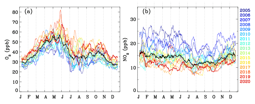
Figure 1 (a) The 2-week moving averages of daytime ground-level ozone concentrations monitored at six sites in Pohang, with (b) corresponding NO₂ concentrations. Different colors represent each year from 2005 to 2020, while the black line represents the mean ozone concentrations from all years.

In wintertime, the annual minimum ozone concentrations have gradually increased by ∼10 ppb during last 15 years, whereas the annual maximum of summertime ozone has rapidly increased from ∼40 to 80 ppb in spite of the reduction of the NO₂ amount by ∼15 ppb or more.

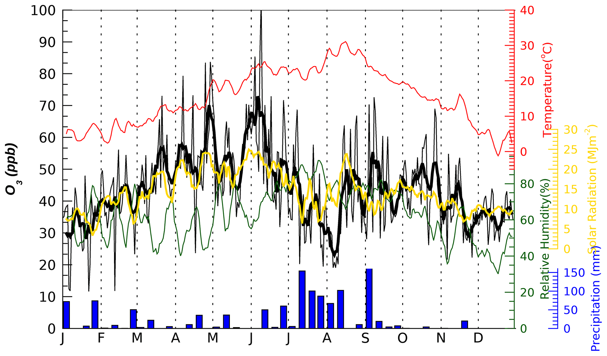
Figure 2 Daily ground-level ozone concentrations (black) with weekly moving averages applied (thick line) or not (thin line) at Pohang in 2020. The corresponding meteorological factors are overplotted: surface air temperature (red, ^∘C), solar radiation (yellow, MJ m⁻²), and relative humidity (dark green, %). The bar graph shows the total precipitation (mm) for each week.

Table 1 Same as Fig. 2, but for correlation coefficients between ozone and meteorological variables for pre-summer, summer, and post-summer periods.

In order to avoid smoothing out important features of intra-summer variations in ozone and their association with synoptic weather patterns, daily ozone and meteorological variables are zoomed in for 2020 as a 1-week moving average (Fig. 2). The local maximum ozone concentrations are generally tied to the local warm, dry air and intense solar radiation before the rainy season starts.

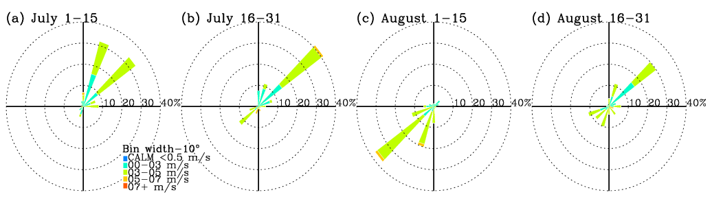
Figure 3 Wind roses for individual months from June through September in 2020 at Pohang. Note that hourly observations in daytime are used to be consistent with data processing done in Figs. 1 and 2.

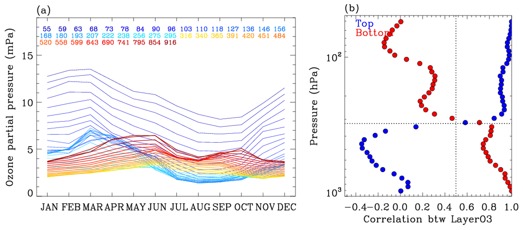
Figure 4 (a) Monthly variations of layer ozone partial pressures from ozonesonde soundings obtained from Pohang during the period of 2005 to 2020. The legend values indicate the midpoint pressure of the layer (hPa). (b) Correlation coefficients of monthly ozone variations between each layer and the bottom layer (916 hPa in red) and between each layer and the top layer (55 hPa in green).

The correlation between ozone concentrations and meteorological variables is quantitatively compared in Table 1 for summer and the post- and pre-summer periods, respectively. Solar insolation amounts are directly linked to ozone concentrations over all seasons (r= 0.51–0.91). The significant relationship between ozone and air temperature is also identified before and after summer seasons. However, in summer, ozone variations are rarely linked with temperature variations due to the intense precipitation suppressing ozone formation. Consequently, the local minimum ozone levels are tied to the local maximum relative humidity during the rainy season ($r=-\mathrm{0.64}$). This indicates that both the depth and width of the summer trough could be highly variable, likely influenced by the strength and duration of the summer monsoon (Yang et al., 2014; Zhou et al., 2022). Note that the relative humidity is significantly influenced by air temperature, rather than the amount of water vapor in the pre- and post-summer periods. Therefore, in post-summer the correlation of ozone with relative humidity (r=0.59) is likely to arise from the correlation of ozone with air temperature (r=0.51). The rapid drop of ∼10 ppb in ozone from the end of July to early August is hardly explained by the meteorological factors mentioned above; the weather becomes warmer with other meteorological variables (precipitation and solar radiation) being relatively invariant. However, the prevailing wind is characterized by southwesterlies in early August, whereas the northwesterly winds were dominant in July and late August (see Fig. 3). This summer minimum could deepen with the inflow of a poor ozone air mass originating from the southern sea off the Korean Peninsula into inland areas.

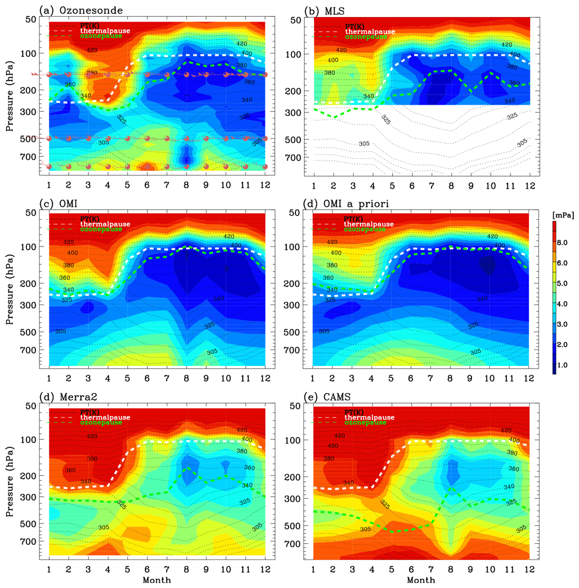
Figure 5 Contour plots of monthly ozone profiles in 2020 from (a) ozonesonde, (b) MLS, (c) OMI, (d) OMI a priori, (e) MERRA-2, and (f) CAMS. The meteorological variables are superimposed for wind barbs (red symbols), potential temperatures (black contours), and thermal tropopause heights (white lines) using monthly MERRA-2 meteorological data. The ozone value of 150 ppb is plotted with green lines to indicate the chemical transition between the troposphere and stratosphere.

3.2 Temporal variability of ozone profiles

To understand the seasonality of ozone profiles, ozonesonde measurements collected at Pohang station are climatologically averaged for each month and each pressure bin (∼0.5 km intervals). Ozonesonde soundings mainly measure ozone in the lower atmosphere below 10 hPa, while space-based limb soundings mainly measure ozone in the upper atmosphere above 215 hPa. However, both sounding measurements provide limited spatiotemporal information. OMI nadir measurements and reanalysis data provide daily global maps of ozone profiles, but the reliability of those data products should be assured before using them to interpret ozone variability and its linkage to the monsoon circulation. As shown in Fig. 4a, two kinds of seasonal patterns are identified with a bimodal structure of layer ozone partial pressures in the lower troposphere (LT), whereas there is a unimodal cycle in the upper troposphere and lower stratosphere (UTLS). The LT ozone concentrations peak in June and October with a global minimum in winter as well as a local summer minimum in late July and early August, which is consistent with surface measurements. The concentrations of UTLS ozone are relatively higher in March due to the stratospheric intrusion, while the minimum concentrations appear broadly over the summer and early fall due to the rise of the tropopause, which is a common feature of ozone in the extratropical UTLS (Gettelman et al., 2011; Rao et al., 2003). In order to quantify the similarity of seasonal variations, the correlation coefficient is calculated for temporal ozone changes between each layer and the top and bottom layer. As shown in Fig. 4b the seasonality of ozone at 50 hPa is significantly correlated down to ∼300 hPa, with a correlation coefficient larger than 0.8. In addition, ozone in the boundary layer is significantly correlated with the lower-tropospheric ozone up to 700 hPa (r>0.9) as well as the upper-tropospheric ozone up to ∼300 hPa (r= 0.7–0.8). This illustrates that 300 hPa could be regarded as a chemical barrier working as a boundary between the troposphere and stratosphere at Pohang.

In Fig. 5, monthly averaged ozonesonde profiles are presented for 2020 and compared as a reference to assess satellite measurements and reanalysis products. This contour map of ozonesondes clearly illustrates the intrusion depth of stratospheric air masses down to ∼300 hPa during spring months (Fig 5a). The mixing depth of ozone that forms near the ground level is also identified, which is bounded up to ∼400 hPa in the summer and ∼600 hPa in other seasons. The minimum ozone concentration is typically found just below the thermal tropopause. The August minimum of lower-tropospheric ozone vertically extends above ∼600 hPa. This air mass is much cleaner compared to the winter ozone concentration over the lower troposphere. The dominant factor suppressing the ozone formation is long-lasting summer precipitation from early July to mid-August in 2020 (Fig. 2). The southerly wind that blows on the observation site is relatively strong compared to June and July. Therefore, we could interpret the inland polluted air masses as likely to be diluted with inflows of maritime clean air masses as mentioned above. In the lower troposphere, a minor peak of ozone concentrations is also identified in spring, which is not visible in time series plots of surface measurements (Fig. 2). The springtime peak is mainly originated by fair weather accelerating the formation of ground-level ozone with the wintertime accumulation of ozone and its processors; it could be partly attributed to the dynamical processes transporting ozone-rich air from the UTLS and upwind areas. In Fig. 5b–f, OMI, MERRA-2, and CAMS ozone profiles are qualitatively evaluated with respect to the capability to reproduce the seasonality of ozone profiles at this location. The ozone minimum of the summer monsoon season is detected from all ozone products, but it is much broader than that in ozonesondes due to both the limited time resolution of ozonesonde measurements and the limited spatial resolution of OMI and reanalysis products. OMI also shows very good agreement with ozonesondes in terms of reproducing the boundary layer ozone extending up to the free troposphere and the low ozone concentration below the tropopause. In addition, the vertical gradient of ozone enhancement above the tropopause is consistently reproduced from OMI, ozonesondes, and MLS. The spring ozone peak near the surface is not detectable from OMI measurements due to the limited sensitivity to relatively shallow boundary layers compared to summer (Shen et al., 2019). In Fig. 5d, an OMI a priori profile is also presented to highlight the fact that the summer minimum is derived from the independent information of OMI measurements rather than a priori information. It also illustrates that the summer minimum is a regional feature of tropospheric ozone seasonality not represented in the climatological data in which long-term global measurements are composited as a function of month and latitude.

Both MERRA-2 and CAMS considerably overestimate ozone abundances in both the troposphere and stratosphere in spite of the fact that MLS measurements are commonly employed for assimilating stratospheric ozone profiles. In MERRA-2, the bimodal peaks (April and October) of the lower-tropospheric ozone are inconsistent with others (early summer, September). We also compare how each ozone product represents the tropopause against thermally defined tropopause heights using the World Meteorological Organization (WMO) definition (WMO, 1957). There is no universal method to define the ozonepause height, but threshold values of 100 to 150 ppb in ozone mixing ratios were used to discriminate stratospheric and tropospheric air masses (e.g., Hsu et al., 2005; Prather et al., 2011). In this paper, the 150 ppb value is selected due to similarities of thermal tropopauses with ozone surfaces of 150 hPa from ozonesonde measurements. As shown, the ozone surfaces at 150 ppb of reanalysis products are positioned in the free troposphere due to the overestimation errors. Both ozonesondes and Aura measurements show some consistency between their ozone and thermal tropopause pressures. In particular, OMI shows strong consistency with the fact that retrievals near the tropopause are largely constrained with the a priori state taken from the tropopause-based ozone profile climatology (Bak et al., 2013).

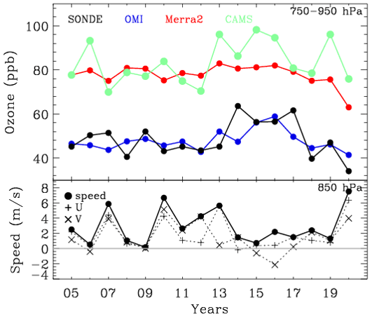
Figure 6 Annual variations of (top) the lower-tropospheric ozone (750–950 hPa) in August from various ozone products, along with (bottom) the wind speeds at 850 hPa.

3.3 Interannual variability of lower-tropospheric ozone in summer

In this section, we focus on the ozone changes related to interannual meteorological variabilities, along with the evaluation of different ozone products. In Fig. 6, time series of the mean ozone mixing ratio in the lower troposphere (750–950 hPa) in August are compared. The summer monsoon typically ends in the late July and early August over the Korean Peninsula, and hence the ozone abundance in August is sensitive to the intensity and duration of the monsoon season. OMI and ozonesondes show a similar long-term change, except for much more fluctuation in time series of ozonesondes due to insufficient samplings (weekly observations) used in monthly averages. A noticeable correlation ($r=-\mathrm{0.52}$) exists between wind speeds and ozone mixing ratios (ozonesonde). Low wind speed could enhance the accumulation of ozone precursors and the rate of ozone formation. Accordingly, both ozonesondes and OMI measurements detect higher ozone abundances in August from 2014 to 2017 when the wind speeds are relatively lower. As shown in Fig. 7a–c, where the monthly meteorological fields at 850 hPa in 2015 are presented from the MERRA-2 product, the western North Pacific Subtropical High (WNPSH) was broken in August, and hence the weather was likely to be calm and dry over the Korean Peninsula. Compared to the past few years, a lower amount of ozone is detected in 2020 from ozonesonde measurements. In August 2020, the lower-tropospheric southwesterly winds blow from the western North Pacific to the Korean Peninsula across the edge of the WNPSH, and the rain belt was activated over the Korean Peninsula (Fig. 7d–f). Therefore, the weather was windy and wet, suppressing ozone formation in August 2020.

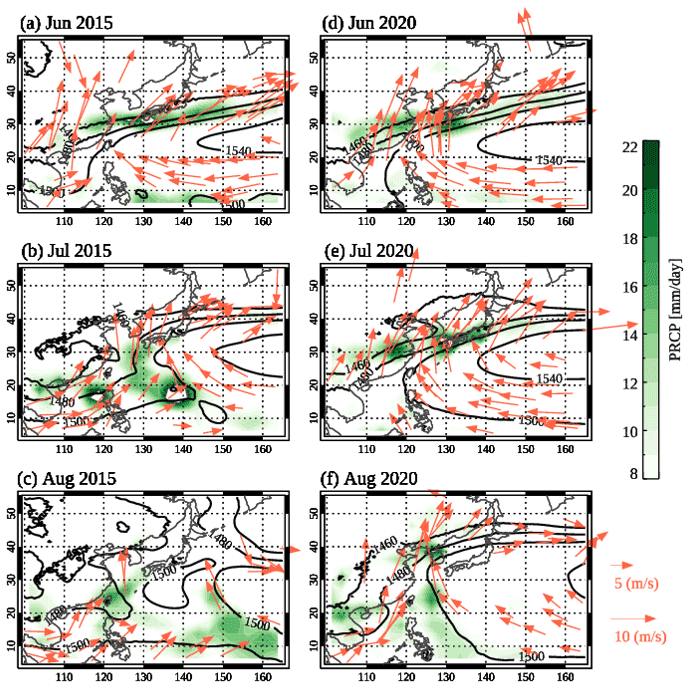
Figure 7 The monthly meteorological fields at 850 hPa for (a–c) 2015 and (d–f) 2020. The wind vectors are drawn with the orange arrows. The geopotential heights are superimposed with black lines. The variations of precipitation are shown in green shades. Note that we use MERRA-2 meteorological variables except for the precipitation data taken from the GPCP Version 2.3 Combined Precipitation Data Set (Adler et al., 2018).

MERRA-2 ozone shows no annual variation before 2020, unlike other ozone measurements and products. CAMS also shows higher ozone concentrations correlated with wind speeds, but these are less consistent with ozonesonde measurements compared to OMI. How the El Niño–Southern Oscillation (ENSO) cycle interacts with the East Asian monsoon has not been established. According to the Oceanic Niño Index, the 2015–2016 El Niño event, the warm phase of the ENSO, was one of the strongest events ever recorded, whereas the 2020–2021 La Niña event was also abnormally strong. There were a lot of unprecedented weather events in South Korea during these super El Niño and La Niña periods, such as unprecedented summer rainfall in 2020 and unprecedented summer heatwaves in 2015–2016 (Yoon et al., 2018). Therefore, we could relate the higher ozone amount in August 2015–2017 and the lower ozone amount in August 2020 to a climatic forcing on the strength and position of the WNPSH and hence the East Asian summer climate.

4 Summary and conclusions

In this paper, atmospheric ozone variabilities over the Korean Peninsula and their linkages to the East Asian summer monsoon are vertically characterized using multiple ozone measurements made by surface observations, balloon-borne ozonesondes, OMI, and MLS. MERRA-2 and CAMS are also integrated in this analysis for the evaluation against ozonesondes. Surface in situ measurements at six urban sites in Pohang are averaged, while satellite and reanalysis datasets are spatially interpolated onto the Pohang ozonesonde site. Surface measurements clearly show the impact of frequent weather changes (dry and wet) on ozone concentrations in spring. The seasonality of ozone becomes very complicated in late spring to early fall, depending on monsoon strengths and lengths. The peak concentration of ozone occurs in the pre-summer monsoon season (∼70 ppb) and in the post-summer monsoon season (∼50 ppb). During the summer monsoon, ozone concentrations decrease down to ∼30 ppb, which is even lower than that in the winter when the air temperature and solar insolation are lowest. The vertical structures of ozone concentrations driven by stratospheric dynamics and synoptic-scale tropospheric weather disturbances are characterized from ozonesonde soundings. Stratospheric intrusions actively occur from March to May and modulate the upper-tropospheric ozone down to ∼300 hPa. We identified ozone enhancements in the boundary layer extending up to 400 hPa in June. In August monsoon-induced ozone dilution occurs in the lower troposphere up to ∼600 hPa. The ozone minimum also occurs just below the tropopause, which is deepest from summer to early fall with the troposphere being extending upward to ∼100 hPa. Both satellite and reanalysis datasets show the capability to reproduce general features of ozone seasonality such as bimodal peaks in ground-level ozone and the spring maximum in UTLS ozone. However, MERRA-2 and CAMS products significantly overestimate ozone abundances in the UTLS, and hence middle-tropospheric ozone concentrations exceed 150 ppb, which is used as a chemical proxy to distinguish between stratospheric air and tropospheric air. In general, OMI shows good agreement with ozonesonde measurements with respect to both seasonal tendency and quantitative terms, but it slightly underestimates ground-level ozone due to the limited vertical sensitivity. The lower-tropospheric ozone in August shows monsoon-induced interannual variabilities with higher concentrations during the super El Niño and lower concentration during the significant La Niña period, which is common from ozonesonde and OMI measurements. However, MERRA-2 rarely shows long-term changes in August ozone in the lower troposphere. On the other hand, CAMS is annually correlated with ozonesonde measurements, but with the systematic positive biases of ∼40 ppb. In conclusion, OMI could play a vital role in studying the impact of summer-monsoon-derived atmospheric circulation and weather on ozone seasonality. The analysis results of this study could be a useful reference for the upcoming results from the ACCLIP campaign performed in the summer of 2022 to gather comprehensive, integrated datasets of two airborne observations (flight operations from S. Korea) as well as ground and balloon measurements over East Asia and the western Pacific. ACCLIP measurements could provide useful ideas for better understanding the spatiotemporal variation of ozone in the Korean Peninsula in terms of continuous ozone increase near the surface (Yoo et al., 2015), high ozone in the free troposphere (Crawford et al., 2021), and the relationship between stratospheric ozone intrusion and atmospheric circulation (Park et al., 2012).