the Creative Commons Attribution 4.0 License.
the Creative Commons Attribution 4.0 License.
 | 03 Nov 2022
Aerosol characteristics and polarimetric signatures for a deep convective storm over the northwestern part of Europe – modeling and observations
Jana Mendrok
Dominik Brunner
The Terrestrial Systems Modeling Platform (TSMP) was extended with a chemical transport model and polarimetric radar forward operator to enable detailed studies of aerosol–cloud–precipitation interactions. The model was used at kilometer-scale (convection-permitting) resolution to simulate a deep convective storm event over Germany which produced large hail, high precipitation, and severe damaging winds. The ensemble model simulation was, in general, able to capture the storm structure, its evolution, and the spatial pattern of accumulated precipitation. However, the model was found to underestimate regions of high accumulated precipitation (> 35 mm) and convective area fraction in the early period of the storm. While the model tends to simulate too high reflectivity in the downdraft region of the storm above the melting layer (mostly contributed by graupel), the model also simulates very weak polarimetric signatures in this region, when compared to the radar observations. The above findings remained almost unchanged when using a narrower cloud drop size distribution (CDSD) acknowledging the missing feedback between aerosol physical and chemical properties and CDSD shape parameters.
The kilometer-scale simulation showed that the strong updraft in the convective core produces aerosol-tower-like features, increasing the aerosol number concentrations and hence increasing the cloud droplet number concentration and reducing the mean cloud drop size. This could also be a source of discrepancy between the simulated polarimetric features like differential reflectivity (ZDR) and specific differential-phase (KDP) columns along the vicinity of the convective core compared to the X-band radar observations. However, the use of narrow CDSD did improve the simulation of ZDR columns. Besides, the evaluation of simulated trace gases and aerosols was encouraging; however, a low bias was observed for aerosol optical depth (AOD), which could be partly linked to an underestimation of dust mass in the forcing data associated with a Saharan dust event.
This study illustrates the importance and the additional complexity associated with the inclusion of chemistry transport model when studying aerosol–cloud–precipitation interactions. But, along with polarimetric radar data for model evaluation, it allows us to identify and better constrain the traditional two-moment bulk cloud microphysical schemes used in the numerical weather prediction models for weather and climate.
- Article
(3961 KB) - Full-text XML
- BibTeX
- EndNote


The effect of aerosol on clouds and precipitation through microphysical and radiative processes remains a major source of uncertainty in weather and climate prediction (Tao et al., 2012; Rosenfeld et al., 2014; Fan et al., 2016). In particular, improved understanding of the microphysical pathways of how aerosol affects cloud evolution (e.g., Rosenfeld et al., 2008; Koren et al., 2008; Yuan et al., 2011; Storer et al., 2014; Jiang et al., 2018; Igel and van den Heever, 2021) and precipitation (e.g., Rosenfeld, 2000; Stevens and Feingold, 2009; Shrestha and Barros, 2010; Li et al., 2011; Guo et al., 2016, 2018) is important for better prediction of extreme events. Many sensitivity studies using numerical models with various degrees of sophistication have been conducted to better understand these microphysical pathways with idealized/semi-idealized (e.g., Khain et al., 2005; Tao et al., 2007; Storer et al., 2010; Lebo and Seinfeld, 2011) or real data simulations (e.g., Noppel et al., 2010; Seifert et al., 2012; Morrison, 2012; Fan et al., 2013; Barros et al., 2018; Fan et al., 2018; Iguchi et al., 2020; Zhang et al., 2021; Trömel et al., 2021). While few of the above sensitivity studies have evaluated the model using radar reflectivity, polarimetric radar data which provide valuable information on cloud microphysical processes have not been fully exploited yet. In most of the numerical modeling studies, the aerosol physical and chemical properties have been held constant, and a large-scale perturbation of aerosol concentrations has been used for sensitivity studies. However, the classical assumptions made for “continental” or “marine” aerosols in the models do not reflect the actual local aerosol type, concentration, and its vertical profile or temporal evolution for any particular region on the globe. In fact, the meteorological settings, land cover, land use, and emissions strongly control the regional spectra of aerosol physical and chemical properties (e.g., Putaud et al., 2010; Martin et al., 2010; Shrestha et al., 2013). More recently, numerical modeling studies with a realistic aerosol distribution obtained by either downscaling region-specific aerosol profiles from a global aerosol model or using a meteorological model online coupled to a chemistry transport model have emerged (e.g., Rieger et al., 2014; Iguchi et al., 2020; Zhang et al., 2021). However, these studies have not fully exploited the potential of evaluating the model simulations against polarimetric radar observations. In this study, we use an online coupled meteorology–chemistry model (Baklanov et al., 2014), the Terrestrial Systems Modeling Platform (TSMP; Shrestha et al., 2014; Gasper et al., 2014) with the Aerosols and Reactive Trace gases (ART; Vogel et al., 2009) module for an ensemble simulation of a summertime deep convective storm over Germany at a kilometer-scale (convection-permitting) resolution. The main goal of the study is to (1) extend the TSMP with a chemistry transport model and a polarimetric radar forward operator to enable detailed studies of aerosol–cloud–precipitation interactions and their evaluation against polarimetric radar observations and (2) to demonstrate these new capabilities for a case study of a deep convective storm over Germany.
The paper is arranged as follows: Sect. 2 describes the observation data, model, forward operator (FO), and model setup used for the study. The first model evaluation of trace gases and aerosols with satellite and ground-based observations is presented in Sect. 3. The modeled aerosol physical and chemical characteristics during the storm event are presented in Sect. 4. The evaluations of modeled cloud microphysical processes and precipitation using polarimetric radar data are presented in Sect. 5. A detailed analysis of polarimetric features and aerosol characteristics is presented in Sect. 6. Finally, discussion and conclusions are presented in Sects. 7 and 8, respectively.
We study a summertime hail-bearing deep convective storm over northwestern Germany. The northeastward propagating storm was associated with the presence of pre-frontal convergence zones developed over this region on 5 July 2015. Scattered storms were prevalent throughout the day, with an isolated deep convective storm passing directly over Bonn from 15:00 to 16:00 UTC on 5 July 2015. Based on observations reported by the European Severe Weather Database (ESWD), large hail (2–5 cm in diameter) was observed over the Bonn region, including damaging lightning further north and heavy precipitation with severe wind (further northeast). A detailed discussion can also be found in Shrestha et al. (2022).
The study region encompasses the northwestern part of Germany bordering with the Netherlands, Luxembourg, Belgium, and France (Fig. 1). The region is characterized by multiple hills of the Rhine Massif, with heights ranging from 600 to 800 m and land cover including forest, agricultural land, and urban/rural area. The region also comprises extensive emissions by point (e.g., oil refineries and other industries) and area sources (e.g., extensive urban and rural areas, road transport, and extensive agriculture; Kulmala et al., 2011; Kuenen et al., 2014), making the region especially suited for this study. Additionally, due to the availability of the twin polarimetric X-band research radars in Bonn (BoXPol) and Jülich (JuXPol) and overlapping measurements from four polarimetric C-band radars of the German Weather Service (Deutscher Wetterdienst, DWD), along with the presence of the Jülich Observatory for Cloud Evolution (JOYCE; Löhnert et al., 2015), the region probably represents the best radar-monitored area in Germany.

Figure 1Spatial pattern of topography over the study region. The Bonn radar domain is outlined in solid line, including the coverage of BoXPol and JuXPol (red circles). The dotted lines indicate the inner domain (excluding the relaxation zone) used to compute the domain average precipitation.
For coupled meteorology–chemistry modeling, we extend TSMP with the ART module. A forward operator is then used to transform the model outputs into radar space for evaluation with polarimetric radar observations from X-band radars. Available satellite observations and in situ observations are also used to evaluate the simulated trace gases and aerosols. A more detailed discussions about the observation data, model, forward operator, and the model setup are presented below.
2.1 Observations
In this study, we use polarimetric radar measurements of hydrometeors and ground/satellite-based estimates of aerosols and trace gases for model evaluation. The polarimetric radar measurements from the twin research X-band Doppler radars located in Bonn and Jülich (BoxPol and JuXPol; Diederich et al., 2015a, b) are used to investigate the microphysical characteristics of the deep convective storm. The polarimetric radar measurements provide valuable information about the horizontal reflectivity (ZH), differential reflectivity (ZDR), specific differential phase (KDP), and cross-correlation coefficient (ρHV), which depend on hydrometeor shape, orientation, density, and phase composition and thus enable a detailed evaluation of the modeled microphysical and macrophysical processes. ZH especially provides information on the size and, with that, on ongoing aggregation/riming processes. ZDR mainly provides information on the shape of hydrometeors and does not depend on the number concentration, while KDP is proportional to the concentration of hydrometeors. ρHV is mainly a measure of the hydrometeor diversity in the resolved radar resolution bin. Different patterns of these polarimetric variables enable us to identify ongoing cloud microphysical processes for precipitating systems. More comprehensive detail about radar polarimetry in general can be found in Ryzhkov and Zrnic (2019), Kumjian (2013), and Trömel et al. (2021), among many others. Further discussions about the polarimetric radar data are available in the Appendix (Sect. A1). Additionally, the RADOLAN (Radar Online Adjustment; Ramsauer et al., 2018; Kreklow et al., 2020) data from the German Weather Service (DWD, Deutscher Wetterdienst) is also used for model precipitation evaluation. RADOLAN is a gauge-adjusted precipitation product based on DWD's C-band weather radars available at hourly frequency in a spatial resolution of 1 km.
For the evaluation of modeled trace gases, remote sensing data from the Ozone Monitoring Instrument (OMI) aboard the Aura satellite is used. OMI provides valuable observations (e.g., O3, NO2, SO2, and HCHO) to better understand the chemistry and dynamics of Earth's atmosphere. In this study, we make use of only OMI NO2 v4.0 data (Krotkov et al., 2019; Lamsal et al., 2021a) to evaluate the spatial pattern of modeled NO2 vertical tropospheric columns (VTCs). Other products were not used due to high uncertainty in their estimates for the timescales of evaluation used in this study. More discussions about the data are provided in the Appendix (Sect. A2).
Similarly, the Moderate Resolution Spectroradiometer (MODIS) 3 km aerosol product (MOD04_L3; Levy and Hsu, 2015) is used to evaluate the simulated spatial pattern of aerosol optical depth (AOD) at 550 nm. In addition, AOD level 2.0 (version 3) ground-based measurements from two AErosol RObotic NETwork (AERONET; Holben et al., 1998; Giles et al., 2019) stations over the domain are also used to evaluate the modeled AOD. These measurements have a better accuracy than MODIS (Giles et al., 2019) but are only available at a few locations.
2.2 Model
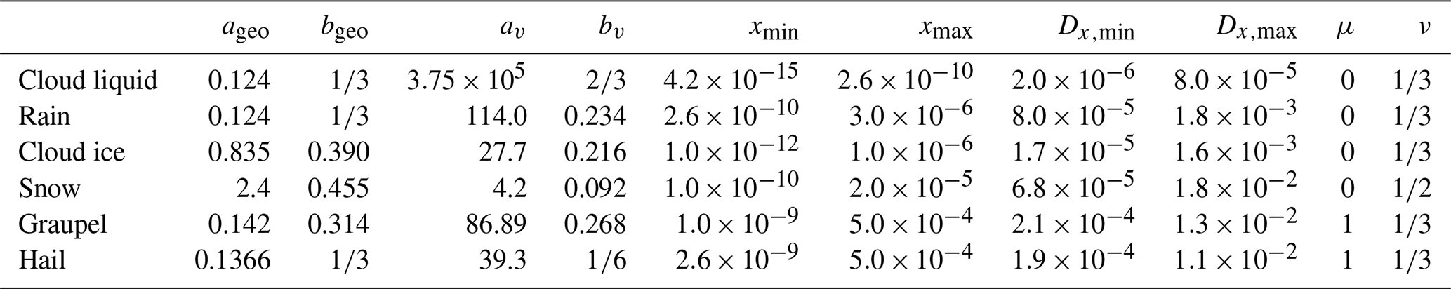
TSMP-ART v1.0 used in this study consists of the atmospheric model COSMO v5.1 (Consortium for Small-Scale Modeling; Steppeler et al., 2003; Baldauf et al., 2011) interfaced with ART v3.1 (Vogel et al., 2009), the land surface model CLM v3.5 (Community Land Model; Oleson et al., 2008), and 3D-distributed groundwater model ParFlow v3.1 (PARallel Flow; Ashby and Falgout, 1996; Jones and Woodward, 2001; Kollet and Maxwell, 2006; Maxwell, 2013). The three component models are coupled using the OASIS3-MCT coupler (Craig et al., 2017). COSMO-ART allows a comprehensive simulation of the two-way interaction between full gas-phase chemistry and aerosol dynamics with atmospheric processes (e.g., aerosol direct and indirect effects; washout of aerosols). Since ART v3.1 is already available as a module for the COSMO v5.1 model (which can be turned on with pre-processor flags), no extensive additional work was required to include the ART module in TSMP. As such, TSMP software was recently updated to include the ART v3.1 module with an extended version of the two-moment bulk microphysics scheme (Seifert and Beheng, 2006), including the hail class (Blahak, 2008, henceforth, SB2M). SB2M predicts the number and mass densities of cloud droplets, rain, cloud ice, snow, graupel, and hail, which are the zeroth and first moments of the particle mass distribution (PMD) that is assumed to follow a modified gamma distribution (MGD), as follows:
with x being the particle mass, and parameters μ and ν determining the shape of the distribution. The specific hydrometeor mass q and specific number n can be derived by and , with ρ being the total density (air, vapor and hydrometeors).
The size–mass and velocity–mass relations of different hydrometeors are parameterized by power laws as follows:
with the (maximum) particle diameter D, terminal fall velocity vT, and parameters ag, bg, av, and bv.
The shape parameters μ and ν of the MGD remain constant for each hydrometeor class, and N0 and λ can be diagnosed from the two prognostic moments. Furthermore, to mitigate the unphysical effects on the mean spectral particle mass coming from the separate advection and sedimentation of q and n, a minimum and maximum allowable mass limit is imposed for (xmin and xmax) at relevant places during the model time stepping. This is done by clipping n so that stays within [xmin,xmax]. For reference, all fixed parameters which were used in this study are summarized in Table 1.
Table 1Parameters of the size–mass and velocity–mass relationships, following Eqs. (2) and (3) used in the SB2M. These refer to D in units of meters, x in kilograms, and vT in meters per second. The last two columns contain the shape parameters of the assumed mass distribution. and are the diameters corresponding to the mass limits xmin and xmax and are added for better interpretation.
When the SB2M is coupled with the ART module, the cloud nucleation parameterization is based on the works of Fountoukis and Nenes (2005), Barahona and Nenes (2007), Kumar et al. (2009), and Barahona et al. (2010). Similarly, the ice nucleation parameterization is based on Barahona and Nenes (2009). A more detailed discussion about the implementation of the above nucleation parameterizations in ART is available from Bangert et al. (2012). The comprehensive activation parameterization works for a parcel of air containing an external mixture of soluble and insoluble aerosols. The activation rate is applied directly for newly formed clouds, while for existing clouds, the activation rate at the cloud base is calculated based on advection and the turbulent diffusion of particles into the cloud base (Bangert et al., 2012). Furthermore, for strong updrafts, in-cloud activation is also computed, for which the growth of existing cloud droplets is considered by assuming that they act as giant cloud condensation nuclei (CCN) that deplete supersaturation (Bangert et al., 2012). The activated aerosols as cloud droplets or nucleated into ice crystals are scavenged and removed. Besides the environmental and microphysical factors, the aerosol activation would also depend on its physical and chemical properties, which varies with elevation in the model. This can contribute to variable partitioning between the interstitial and activated aerosols as cloud droplets. Also, the parameterizations for the direct aerosol effect on the radiation and washout of aerosols by precipitation was turned on for the simulations. These formulations are all based on the prognostic aerosol population with 12 overlapping modes simulated in ART. Each mode is approximated by a lognormal distribution with uniform chemical composition across size. The 12 modes consist of the nucleation and accumulation mode for pure and mixed aerosol particles (sulfate, ammonium, nitrate, organic compounds, water, and soot), small, medium, and large particles for dust and sea salt, soot particles, and coarse particles (not used for the nucleation parameterization). These aerosol modes are coupled with gas-phase chemistry and strongly influenced by the atmospheric boundary layer evolution, advection, and anthropogenic emissions of gases and particles. An additional overview about the individual aerosol modes, chemical composition, and cloud interaction processes along with the aerosol dynamical processes can be found in Bangert et al. (2012).
For input of emission inventories, the online emission module developed earlier by Jähn et al. (2020) is used. This module makes use of pre-processed inventory data projected onto the model grid along with temporal and vertical scaling profiles for individual emission categories. A more detailed discussion about the pre-processing of emission inventories is presented in Sect. 2.4.
2.3 Forward operator
EMVORADO, the Efficient Modular VOlume scanning RADar Operator (Zeng et al., 2016) is COSMO's native radar forward operator. The FO uses model states and assumptions about the prescribed hydrometeor physical properties to compute the polarimetric radar variables, which are observed by X-band radars. FO requires consistency with the model, particularly regarding hydrometeor microphysics, i.e., size distributions and mass–size and velocity–size relations. For the online version run simultaneously with COSMO, this is ensured completely through variables shared between the modules. For an offline version run, this consistency is maintained manually. Here, we make use of the offline version, though, which is more flexible and allows us to re-run the FO with varied in-FO assumptions for, e.g., sensitivity analyses. More details about the FO is available in the Appendix (Sect. A3).
2.4 Model setup
The simulation is set up for an approximately 340 km × 340 km wide Bonn radar domain (Shrestha, 2021a) at a kilometer-scale resolution for the period 4 to 5 July 2015. For the initial and lateral boundary condition (IC/BC) of the atmospheric states in COSMO, data from the COSMO-DE ensemble prediction system (EPS; Gebhardt et al., 2011; Peralta et al., 2012) are used. The EPS data represent uncertainties in model physics and lateral boundary conditions by combining five model physics perturbations with four global models. An earlier study by Shrestha et al. (2022) showed that the statistics of the EPS are always stratified according to the four global models; i.e., the five members having the same global model are more similar to each other. In this study, we therefore only employ those five ensemble members that are based on the same global model of DWD (GME; Majewski et al., 2002). The ensemble simulation is used to reduce the uncertainty associated with meteorological forcings. The initial soil–vegetation states for CLM and ParFlow are obtained from spinups using offline hydrological model runs over the same domain (Shrestha, 2021a). For the initial and lateral boundary condition of trace gases and aerosols, we use the 6 h data from Model for Ozone and Related chemical Tracers, version 4 (MOZART-4; Emmons et al., 2010). The MOZART-4 data are available at a resolution of 1.9∘ × 2.5∘ with 56 levels. The COSMO model Processing Chain version 2.2 (available at https://github.com/C2SM/processing-chain, last access: 1 January 2022) was used for the pre-processing of the MOZART-4 data into ART variable states. This Python script maps the gases and aerosols (mass concentrations) from MOZART-4 to ART state variables. For the initialization of the number concentration of each aerosol mode, the default density and initial mode diameters in the ART module are used. Furthermore, we also assume that the aerosol has been in the atmosphere for a long time, where it could coagulate and mix, so 0.1 % and 99.9 % of the fine mode aerosols are assigned to mixed nucleation and accumulation mode, assuming a median diameter of these modes of 50 and 150 nm, respectively. The mapping from MOZART-4 to ART aerosol classes and the assumptions regarding median diameters are an additional source of uncertainty in the initialization of aerosols in the model.
The Copernicus Atmosphere Monitoring Service – Regional Inventory v4.2 (CAMS-REG v4.2; Kuenen et al., 2022) was used to prescribe the spatiotemporal emissions for the study. CAMS-REG v4.2 is a state-of-the-art gridded anthropogenic emission inventory developed for the European domain at a 0.1 ∘ × 0.05 ∘ grid resolution, with a temporal coverage of 18 years (2000–2017). This emission inventory was pre-processed using the Python package “emiproc” (Jähn et al., 2020), available publicly through the C2SM GitHub organization (https://github.com/C2SM-RCM/cosmo-emission-processing, last access: 22 October 2022) for COSMO-ART variable states. First, the emission inventory data are projected onto the model grid, and then the temporal and vertical scaling profiles for individual emission categories are estimated. These inputs are then read during the model initialization, and the temporal and vertical emission profiles per category are applied online during the model run. In addition, the land cover data from Global Land Cover Map for 2009 (GlobCov 2009; Arino et al., 2012) is used for the biogenic volatile organic carbon (VOC) emissions. Furthermore, there is no emission of dust inside the model, and dust only comes from the MOZART-4 boundary conditions.
The ensemble simulation starts on 4 July 2015 at 06:00 UTC, and the model is integrated for 42 h. In all runs, a coupling frequency of 90 s is used between the atmospheric and hydrological components, which have a time step of 10 and 90 s, respectively. The model is integrated over the diurnal scale, and the output is generated at 5 min intervals and hourly intervals for evaluation with polarimetric radar data (only for a 3 h period) and aerosol measurements, respectively.
First, the modeled trace gases and aerosols are evaluated with satellite- and ground-based observations. For comparison, the model data were also cloud screened. A threshold of 20 g m−2 was used for the total column-integrated liquid and ice condensate for the cloud screening.
The vertical tropospheric column (VTC) is used to compare simulated NO2 with satellite estimates from OMI. The VTC is an integral measure of the tracer from the surface to the tropopause. While it can be readily estimated from the model, the satellite estimates are dependent on the assumed vertical profiles of NO2 in their algorithms. We acknowledge this uncertainty in the satellite estimates and the corresponding limitations of a direct comparison with the model data. However, it has to be stressed that this comparison is a very limited evaluation, since we are comparing the model with observations for a single day only. Both the satellite and the modeled VTC for NO2 exhibit similar patterns, with relatively higher magnitudes over the northwestern lowlands and lower magnitudes over the Rhine Massif around 4 July 2015 at 12:00 UTC (Fig. 2). However, the model exhibits relatively higher magnitude of NO2 over the foothills of the Rhine Massif near the emission sources (mostly from the mining regions and industry northwest of Bonn), which is not captured in the satellite retrievals. In order to compare simulated and observed NO2 VTCs more quantitatively, we also interpolated the model output over the individual OMI pixels using an inverse distance squared algorithm (not shown here). The model exhibited a correlation coefficient of 0.46 with the observation.
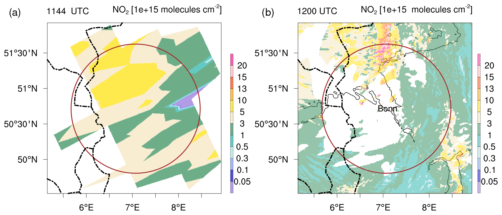
Figure 2Satellite (a) and model (b) estimates of integrated vertical tropospheric column (VTC) for NO2 over the Bonn radar domain on 4 July 2015.
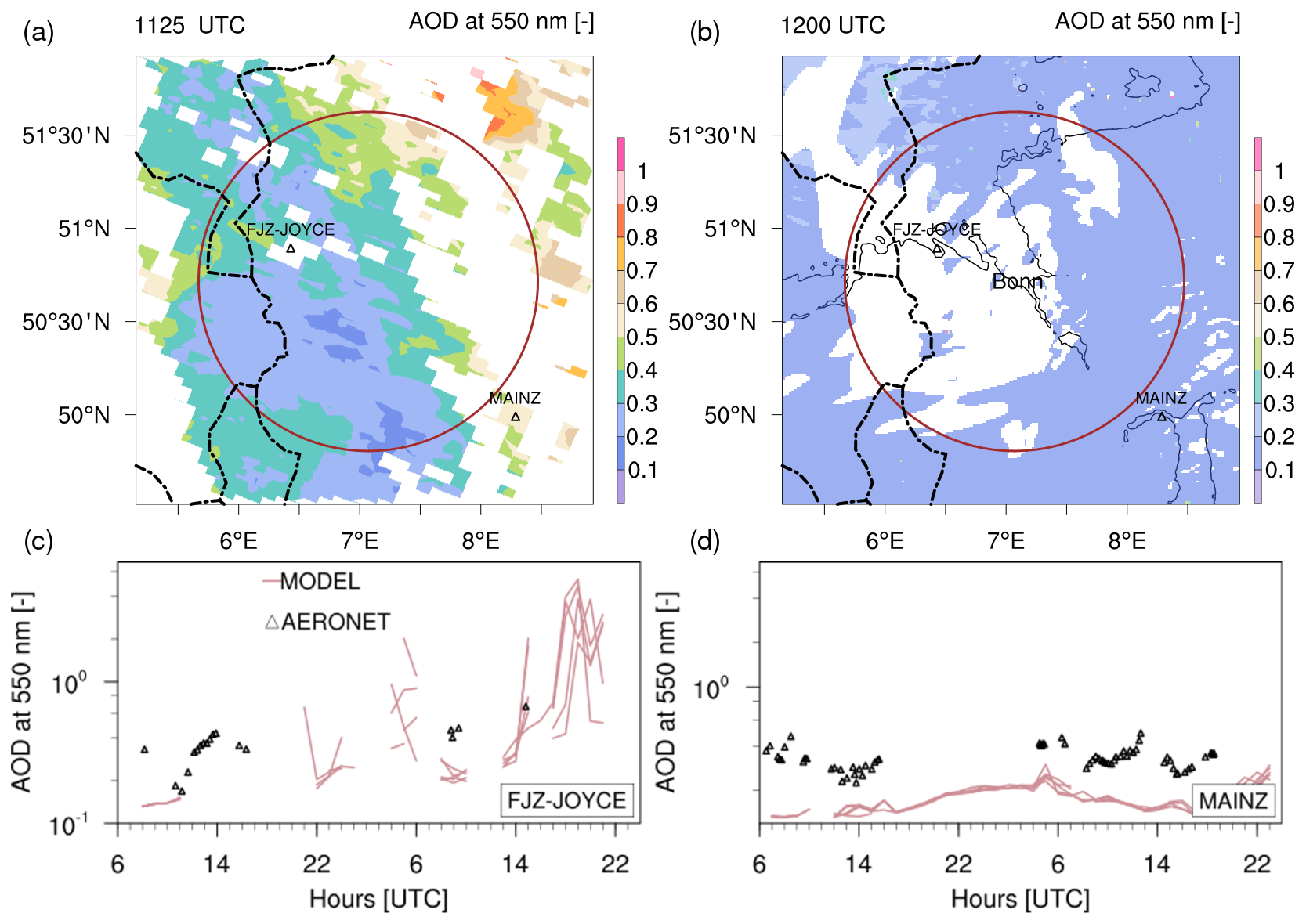
Figure 3(a–b) Satellite and model estimates of aerosol optical depth (AOD at 550 nm) over the Bonn radar domain on 4 July 2015. The two available AERONET stations over the Bonn radar domain are also shown. (c–d) Time series of measured and simulated ensemble AOD over FJZ-JOYCE and MAINZ AERONET stations.
The modeled aerosol optical depth (AOD) is also compared with satellite retrievals from MODIS. In comparison with the MODIS data on 4 July 2015, the model tends to simulate relatively low AOD (0.1–0.3) over most of the domain (Fig. 3a–b). The MODIS data also show low AOD (0.1–0.3) over large parts of the domain but with pockets of high AOD scattered over the northern parts, which is not captured by the model. This bias in the modeled AOD can also be observed when comparing the modeled AOD with available AERONET station data over the region. The model generally tends to underestimate the AOD as estimated by the in situ measurements (when available). This is more prominent for the MAINZ station (Fig. 3d). However, within the spread of the ensemble members, the model also tends to the capture measured AOD over some period of times at Forschungszentrum Jülich (FZJ)-JOYCE station (Fig. 3c). In general, the above model evaluation with satellite data and ground-based measurements do build some confidence over the modeled aerosol and gaseous species.
The modeled evolution of aerosol physical and chemical properties during the convective storm event are summarized in Figs. 4 and 5, respectively. Two different time periods are chosen as the storm propagates toward northwest, with strong updrafts in the synthetic sampling location at 15:00 UTC. The aerosol number concentrations of different modes (Nx) exhibit a strong variability in space and time. Figure 4a shows the spatial pattern of number concentrations of the sum of nucleation and accumulation mode for both pure and mixed aerosols (Nna) at 2 km height on 5 July 2015 at 14:00 UTC. At this time, the sampling location exhibits relatively low Nna compared to the western part, which has an extended patch of high Nna with an east to west extent. Over the next hour, this patch appears to be advected northwest, owing to the dominant southwesterly wind direction (Fig. 5a). At the same time, the spatial propagation of convective updrafts also plays a crucial role in lifting of aerosols to 2 km altitude. The evolution of the spatial pattern thus appears to be determined by a combination of horizontal advection and vertical updraft, with the latter additionally depending on the co-location with local emissions. Figure 4b shows the average aerosol size distribution for different modes and PM2.5 (particulate matter with size <2.5 µm) chemical composition for a 9×9 grid cells box encompassing BoXPol at the center. At 2 km height, the dust particles dominate the aerosol mass, while soluble components make up only about 26 %. As expected, Nna is highest near the surface and generally decays with height. The magnitude of Nna is around 180 cm−3 at 2 km level. Also, a rightward shift in the aerosol size distribution of nucleation/accumulation mode can be observed that is associated with fresh aerosols near the surface and more aged aerosols in upper layers, with a larger mode at around 300 nm. The soot particles exhibit a multi-modal distribution with larger mode around 200 nm, while the dust particles exhibit a larger mode around 2000 nm. Figure 4c shows the meridional cross section of the aerosol number concentration (Nx) for a combination of different aerosol modes. As observed in the aerosol size distribution (Fig. 4b), Nna and Nsoot exhibit higher concentration below 3 km height. Localized high values of Nna along the cross section are associated with local emissions. The dust aerosols exhibit a more horizontally homogeneous profile with a peak around 4 km, which is probably associated with a Saharan dust event. The multi-model forecast of dust from World Meteorological Organization (WMO) Barcelona Dust Regional Center (https://dust.aemet.es/products/daily-dust-products, last access: 22 October 2022) indicates the presence of Saharan dust for this particular event. The PM2.5 concentration also shows peaks near the surface and near the melting layer but is associated with the Nna and Ndust, respectively.
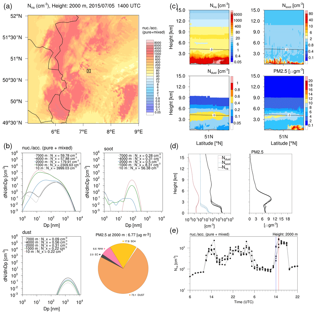
Figure 4(a) Spatial pattern of the aerosol number concentration for nucleation/accumulation (nuc./acc.; pure + mixed; Nna) at 2000 m height on 5 July 2015 at 14:00 UTC. The square with the “x” symbol at the center indicates the sampling location east of BoXPol, with the extent of a 9×9 box. (b) Average aerosol size distribution of different modes and PM2.5 concentration for the 9×9 box. (c) Meridional cross section of the aerosol number concentration and PM2.5 concentration passing through the sampling location. Also shown is the 0 ∘C isotherm. (d) Ensemble vertical profile of aerosol number concentration for nuc./acc. (pure + mixed; Nna), soot (Nsoot), dust (Ndust), and PM2.5 concentration at “x”. (e) Ensemble time series of aerosol number concentration for nuc./acc. (pure + mixed) at 2000 m height at the BoXPol location. The blue and red lines correspond to times at 14:00 and 15:00 UTC, respectively.
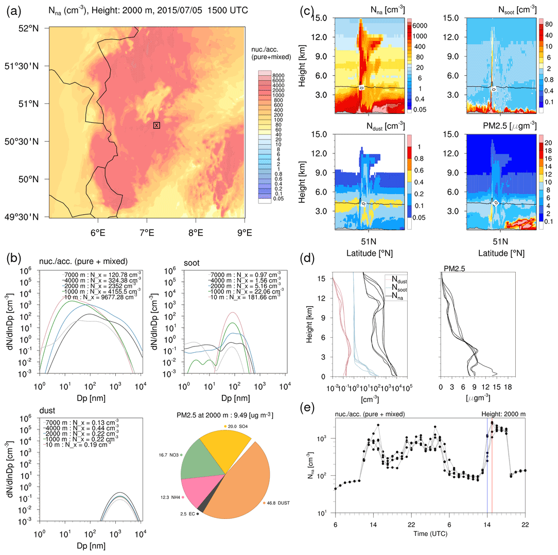
Figure 5Same as Fig. 4 but on 5 July 2015 at 15:00 UTC.
Figure 4d shows the area average vertical profile of the aerosol number concentration for different modes. The profiles are shown for the same 9×9 grid cells for five ensemble members. In general, all ensemble members exhibit similar profiles for this time period. Importantly, the aerosols exhibit a strong diurnal cycle owing to emissions, atmospheric boundary layer (ABL) evolution, updraft, and advection (Fig. 4e). At 2 km height, it generally peaks during the day and decays during the night (here only shown for nucleation/accumulation, nuc./acc., mode), except for periods with persistent convection or advection of aerosols. The situation at 15:00 UTC, when the aerosol distribution is strongly influenced by the deep convective event, is illustrated in Fig. 5. Due to the strong updraft associated with the convective storm, the aerosol size distribution of the nucleation/accumulation mode has become much broader (especially at 2–4 km height) as compared to the situation at 14:00 UTC. At the same time, the aerosol number concentration has increased, and the chemical composition (Fig. 5b) has changed significantly. The aerosol solubility and PM2.5 mass concentrations at 2 km height have increased rapidly from 26 % to 46 % and 6.77 to 9.49 µg m−3, respectively. The simulated strong updraft over the sampling location also appears to generate localized aerosol towers reaching up to 15 km height (Fig. 5c). This increases the aerosol number concentration for all modes rapidly at higher altitudes (see Fig. 5d). We further discuss about these aerosol towers with polarimetric variables in following sections. In general, the variability in the location and magnitude of the simulated updraft associated with the convective storm produces the spread in the ensemble members.
First, the modeled daily accumulated precipitation (5 July 2015) is evaluated with estimates from RADOLAN. Figure 6a–b show the spatial pattern of ensemble-averaged and RADOLAN-accumulated precipitation. In general, the model is able to capture the spatial pattern of the observed precipitation. However, the model underestimates the high precipitation in the northeastern part of the Bonn radar domain. This underestimation is also seen in the frequency distribution of the simulated and observed accumulated precipitation (Fig. 6c). While the domain average precipitation is similar to the RADOLAN data, all ensemble members tend to underestimate regions with high accumulated precipitation (> 35 mm). But, all ensemble members tend to slightly overestimate medium accumulated precipitation (10 to 30 mm).
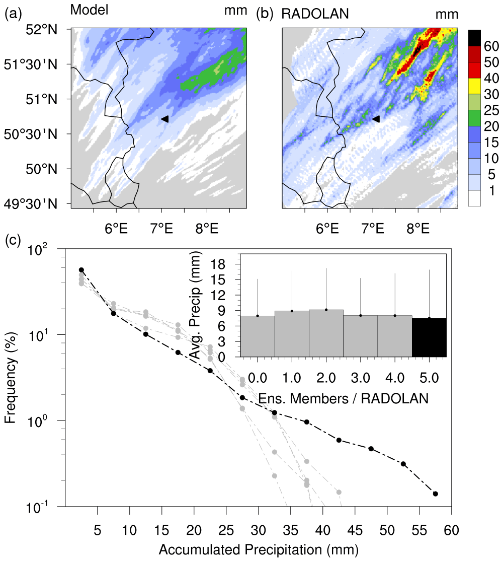
Figure 6Spatial pattern of accumulated precipitation. (a) Ensemble average from the model. (b) RADOLAN estimates. The black marker shows the location of BoXPol. (c) Frequency distribution of the simulated and observed accumulated precipitation. The inset shows the domain-averaged accumulated precipitation for each ensemble member (light gray color bar) and observation (black color bar) with 1 standard deviation (solid line above the bars).
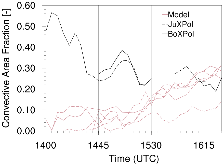
Figure 7Convective area fraction (CAF) of model ensemble members and observations. The two vertical bars define the time period used to compute contoured frequency altitude diagrams (CFADs) for the observation and model. The ensemble member, with a solid line, is used for polarimetric signature comparison. The CAF estimates from BoXPol or JuXPol are shown upon coverage and data availability. The gaps in the radar data represent times when the polarimetric signatures are strongly attenuated or if the storm extent is only partially covered by the radar.
The underestimation of high accumulated precipitation indicates that the model underestimates the high precipitation amounts associated with the core of the convective storm. This is also well seen in the time series of the convective area fraction (CAF; Fig. 7), which is estimated as the ratio of the storm area at 2 km above ground level (a.g.l. hereafter) with ZH > 40 dBZ to the total area with ZH > 0 dBZ. The masked storm area is generated using a storm tracking algorithm, which uses edge detection and overlapping areas between consecutive snapshots to track the storm. Observations from JuXPol and BoXPol exhibit high values of CAF in the early period of the storm (14:00 to 15:30 UTC), which is underestimated by all ensemble members. The ensemble members exhibit a similar pattern with increasing CAF after 15:30 UTC, when the simulated CAF matches the observed CAF more closely. However, such direct comparisons are always challenging due to mismatches in simulated and observed storm evolution in space and time, so we also conducted a qualitative exploratory analysis (using synthetic polarimetric variables at a lower altitude (1 km a.g.l.), near the melting level (4 km a.g.l.), and at a higher altitude (7 km a.g.l.) to find simulated convective storm structures closer in time and space to the radar observations. Based on this analysis, we compare the polarimetric signatures of the storm between one of the ensemble members (solid line; Fig. 7) and the BoXPol observations at 15:30 UTC.
Figure 8a) shows the plan position indicator (PPI) of polarimetric variables at 8.2∘ elevation from BoXPol measurements. Near the melting level, the storm is characterized by high reflectivity (> 50 dBZ) and differential reflectivity (> 2 dB). At upper levels (beyond the convective core), the storm exhibits reflectivity in the range of 15 to 25 dBZ. The inflow region of the storm lies in the southeastern corner, which has relatively lower ρHV but high ZH and ZDR. The storm also exhibits an arc-like feature of high ZDR along the eastern edge. Figure 8b shows the vertical cross section of the same polarimetric variables based on the gridded radar data along a north–south transect through the storm center. The convective core extends from −20 to 5 km, exhibiting high reflectivity (> 50 dBZ) from the surface up to 6 km height. A well-defined ZDR column (> 2 dB) anchored to the surface and extending up to 6 km height is also visible along the cross section. ZDR columns are distinct polarimetric signatures often found along the vicinity of the strong convective updraft core (Kumjian and Ryzhkov, 2008; Kumjian et al., 2014; Snyder et al., 2017b). KDP columns (Ryzhkov and Zrnic, 2019; Snyder et al., 2017b) are also clearly distinguishable and co-located with ZDR columns with slight inward offsets. High ZDR and KDP above the melting layer often indicate the presence of frozen raindrops, water-coated hail, and large size supercooled raindrops (Kumjian et al., 2014; Ryzhkov and Zrnic, 2019). Below the melting layer in the convective region, KDP also has high magnitudes contributed by the melting of graupel/hail into raindrops. The high reflectivity values in the convective core with low ρHV (< 0.92) also indicates the dominance of the hail signature.
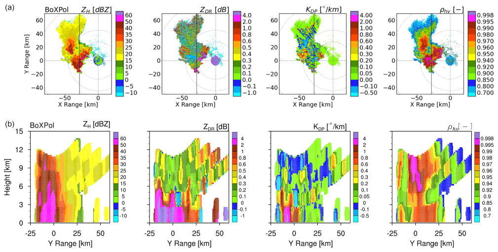
Figure 8(a) Plan position indicator (PPI) plots of the horizontal reflectivity and differential reflectivity, specifically, the differential phase and cross-correlation coefficient at 8.2∘ elevation measured by BoXPol on 5 July 2015 at 15:30 UTC. The dotted gray circles represent slant ranges for the chosen elevation angle, associated with heights of 1 km (lower level), 4.5 km (melting level), and 7 km (upper level). (b) Cross section of the same polarimetric variables from the gridded data. The vertical solid black line along the Y range in panel (a) indicates the location of the cross-sectioned plots.
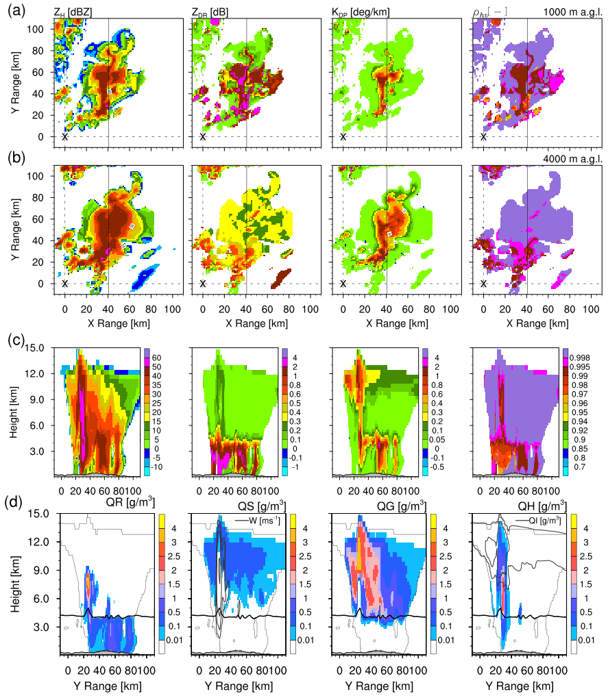
Figure 9(a, b) Model-simulated horizontal reflectivity and differential reflectivity, specifically, the differential phase and cross-correlation coefficient at the low-level (1000 m a.g.l.) and near-melting layer (4000 m a.g.l.) on 5 July 2015 at 15:30 UTC. The “x” symbol refers to the BoXPol location. The gray solid line indicates the location of the cross section. (c) Cross section of the same polarimetric variables. (d) Cross section of model-simulated hydrometeor density (QR is rain, QS is snow, QG is graupel, and QH is hail). Also shown is the 0 ∘C line (solid black line) indicating the melting layer, contours of vertical velocity (5, 10, 20, 40 m s−1) with QS, and contours of cloud ice density (QI) with QH.
Figure 9a–b show the spatial pattern of the synthetic polarimetric variables for the storm at 1 and 4 km a.g.l, as derived from the model simulation. Compared to the observations, the storm is already ahead of the BoXPol location but exhibits a similar structure compared to the observations. At lower levels (1 km a.g.l.), the storm exhibits an elongated zone with ZH > 40 dBZ, which is also associated with relatively high ZDR, KDP but relatively lower ρHV. Near the melting level, the extent of the region with ZH > 40 dBZ is much wider and also partly associated with high values of KDP. However, relatively high values of ZDR and lower values of ρHV are mostly constrained around the convective core. The meridional cross section of the synthetic polarimetric variables show that the storm top extends up to 13 km height, with an overshooting top up to 15 km height (Fig. 9c). The convective core also exhibits reflectivity > 50 dBZ up to 10 km height but is relatively narrow compared to the observation. A ZDR-column-like feature protruding on top of the melting layer and anchored to the ground is also simulated; however, its magnitude is less than 0.8 dB. This is much weaker than the observed ZDR columns with a magnitude of > 2 dB. Above the melting layer, ZDR is generally weak (0 to 0.1 dB), with slightly higher values along the convective core. KDP also exhibits relatively high values in the convective core, extending up to the storm top. ρHV is also relatively lower in the convective region and below the melting layer. In general, there is lack of polarimetric signal above the melting layer in the downdraft region of the storm, similar to an earlier study by Shrestha et al. (2022). The low variability and high values of synthetic ρHV can be attributed to the shortcomings in the FO assumption of the hydrometeor shape and orientation (Shrestha et al., 2022). The lack of a polarimetric signature in the downdraft region of the storm above the melting layer could be due to the deficiency in the FO for correctly modeling the scattering properties of snow and graupel which dominate this region, as discussed below.
The meridional cross section of the modeled hydrometeors shows the presence of supercooled raindrops in the strong updraft region, where the modeled vertical velocity above 8 km reaches 40 m s−1 (Fig. 9d). The strong updraft also generates a warm anomaly above the melting layer (see the 0 ∘C isotherm), below which rain is mainly produced by melting of graupel and hail. The melting of graupel and hail into raindrops produces the high KDP below the melting layer. For ice hydrometeors, graupel dominates, with high-density surrounding the convective core. Graupel is responsible for the high reflectivity in the downdraft region of the storm above the melting layer. Cloud ice is located mostly above 8 km height and contributes to the high KDP near the storm top. The self-collection of these ice particles leads to the formation of snow which extends further down to 6 km as it grows in size via aggregation. Hail mostly dominates in the strong updraft region of the storm with peaks in mass density adjacent to the supercooled raindrops. It also contributes to the high ZDR values simulated in the convective region above the melting layer. The mean diameter of the supercooled raindrops is only around 0.1 to 0.3 mm, and the above-observed ZDR-column-like signature is produced by the presence of water above freezing level due to melting of hail only. The mean hail size ranges from 0.1 to 13 mm (e.g., around 6 km height). During this time, the hail is also reaching the ground, starting from 15:25 to 15:40 UTC. In general, the ZDR column usually appears 15–20 min before the hail reaches the ground (Ilotoviz et al., 2018). So, we also additionally explore this polarimetric feature in detail at earlier times in the following sections.
While the above analysis already indicates some shortcomings in the synthetic polarimetric signatures, the uncertainty due to mismatches between the space and timescales of synthetic and observed polarimetric variables also needs to be addressed by monitoring ensemble properties of the convective storm. So, additionally, the synthetic polarimetric variables from the ensemble simulations are compared to the observations from 14:45 to 15:30 UTC (see Fig. 7) using contoured frequency altitude diagrams (CFADs; Yuter and Houze, 1995) using the same extents and bin widths.
Figure 10a shows the CFADs of the polarimetric variables from BoXPol measurements. ZH exhibits a narrow distribution at upper levels, with peaks around 15 to 25 dBZ. The distribution gradually broadens from the mid levels to the ground, with peaks around 15 to 40 dBZ near the melting layer. ZDR has a narrow unimodal distribution above the melting layer with a peak around 0.14 dB. The distribution gradually broadens below the melting layer, with peaks shifting to 0.62 dB near the lower levels. KDP also has a very narrow unimodal distribution with peak around 0.1 ∘ km−1. The distribution does exhibit a weak broadening from 8 km towards the surface. ρHV exhibits a broader distribution with peaks around 0.97 to 0.99 up to 10 km height. Above, the peak shifts towards 0.82 to 0.85.
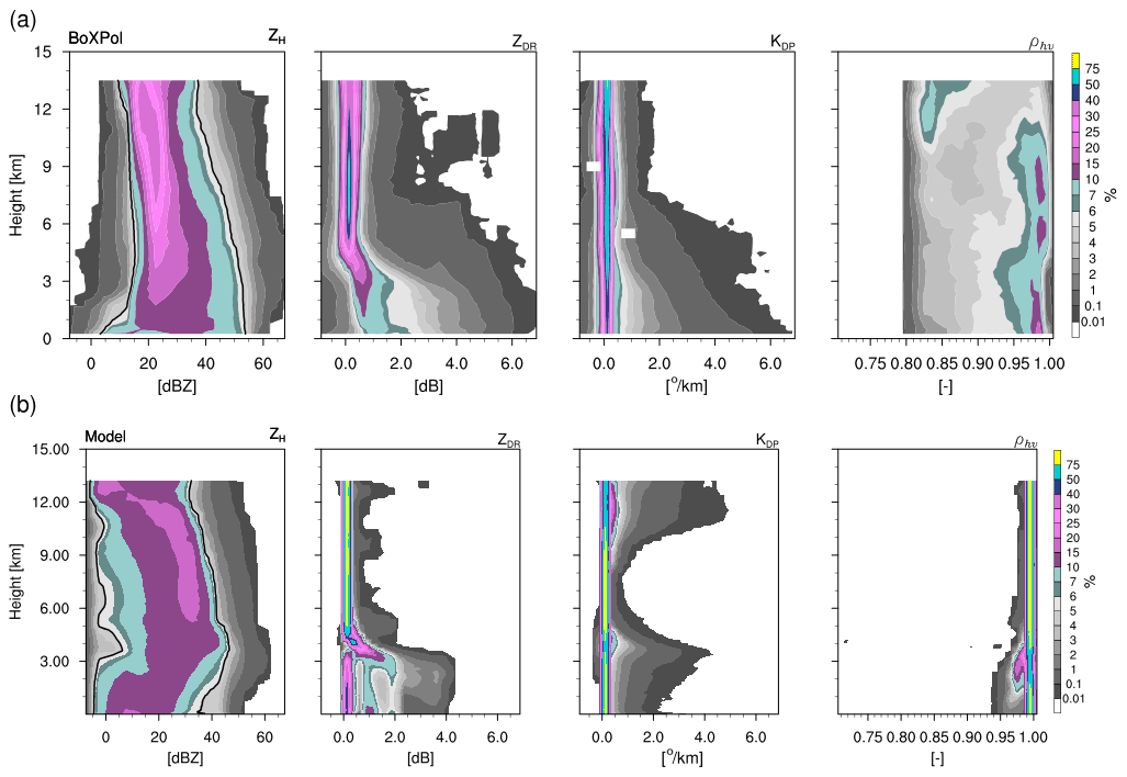
Figure 10CFADs of horizontal reflectivity and differential reflectivity, specifically, the differential phase and cross-correlation coefficient from 14:45 to 15:30 UTC on 5 July 2015. CFADs from the model are shown for five ensemble members.
Compared to the observations, the ensemble CFADs of synthetic ZH exhibit a relatively broader distribution, with peaks around 20 to 35 dBZ in the upper levels. The peak of the distribution gradually shifts rightwards (30 to 40 dBZ) near the melting layer. Below the melting layer, the peak of the distribution shifts leftwards (3 to 25 dBZ), which also explains the lower CAF from the ensemble members compared to observations during this period. Similar to observations, synthetic ZDR has a narrow distribution above the melting layer, with a peak around 0.11 dB. The distribution gradually broadens below the melting layer with additional peaks at around 1 and 2 dB. Similar to observations, synthetic KDP has a very narrow unimodal distribution with a peak around 0.12 ∘ km−1. It also exhibits a weak broadening in the storm-top region and near the melting layer. For synthetic ρHV, the ensemble model CFADs show a very weak variability, with a peak at around 0.99 and a slight broadening below the melting layer.
The observations from X-band radar show the ZDR and KDP column as being one of the distinct features of this storm. However, the model is only able to simulate comparatively weak polarimetric features and contrasting aerosol-tower-like features. These polarimetric features and aerosol characteristics are therefore also explored for an earlier time at around 15:00 UTC. This time was chosen because it is also 25 min ahead of the hail reaching the ground and due to the availability of additional aerosol data (due to hourly output).
Figure 11a–b show the spatial pattern of ZDR at 6 km height, along with the vertical wind speed. Enhanced ZDR is present, surrounding a strong convective core. The width of the core is around 12 km, with the vertical speed exceeding 30 m s−1. The forward flank downdraft and the rear flank downdraft is also visible. The meridional cross section shows the presence of a warm temperature perturbation above the melting layer in the convective core, which is mainly responsible for the melting of hail in the FO at relatively higher level, producing the ring-like ZDR feature around the convective core.

Figure 11Plan view (a) and vertical cross section (b) of aerosols, model states, and polarimetric variables. The plan views are shown at 6 km height, and all cross sections passing through the solid line are shown in the plan view. The 0 and −10 ∘C isotherm is also shown in all cross sections. (a, b) Differential reflectivity (color fill) and vertical velocity (lines). The contoured solid/dashed red/blue lines indicate updraft and downdraft, respectively. The vertical wind speed contours are shown at the following intervals (−7.0, −5.0, −3.0, −1.0, 5.0, 10.0, 15.0, 20.0, 25.0, 30.0, 35.0, 40.0) in meters per second. (c, d) Rain and hail mixing ratios in filled and solid line contours, respectively. (e, f) Aerosol and cloud number concentrations in filled and dashed line contours, respectively. The cloud number concentration is contoured at interval of 500 cm−3, with a minimum of 100 cm−3. The aerosol concentration is shown for the pure and mixed nucleation and accumulation model aerosols.
The simulated ZDR signal is mostly produced by the raindrops and hail particles (Fig. 11c, d). Raindrops dominate the convective core (above the melting layer) and downdraft region (below the melting layer) in terms of mass density. Hail mostly peaks northwest of the strongest convective core and also extends partly to the downdraft region above the melting layer. Above the melting layer in the convective core, the mean raindrop size is only around 0.1 to 0.3 mm, while the southwestern region exhibits grid-scale supercooled raindrops with size range of 1–3 mm, but part of its polarimetric signal is also masked by hail in the FO. The mean size of raindrops below the melting in the downdraft region is around 1 to 3 mm, which contributes strongly to the ZDR signal besides the contribution from melting hail. The mean size of the hail particles is generally around 1 to 13 mm, with peak values around 6 to 9 km.
The comparatively small mean size of the hail particles and raindrops in the convective core could be due to the very high cloud drop number concentration simulated in the model (Fig. 11e, f). The cloud drop number concentration exhibits strong co-variability with the simulated nucleation/accumulation mode aerosol number concentration (Nna). The strong updraft increases the aerosol load in the convective core, which increases the aerosol number concentration and, consequently, the cloud drop number concentration, which varies from 100 to 3000 cm−3, leading to a very small size of cloud drops ranging from 5 to 25 µm.
In this study, we extended the state-of-the-art terrestrial systems modeling platform with a chemistry transport module and a polarimetric forward operator. The model was then used to evaluate synthetic polarimetric signatures of a deep convective storm event over Germany with observations from X-band radar to better understand aerosol–cloud–precipitation interaction.
The model was also evaluated with satellite- and ground-based observations of trace gases and aerosols. The spatial pattern of NO2 VTC was well captured by the model. This is consistent with an earlier evaluation of COSMO-ART by Knote et al. (2011), who also showed that the model was able to capture the spatial pattern and magnitudes compared to OMI estimates over Europe. Their study also showed that COSMO-ART underestimated the summertime AOD over much of Europe, compared to the estimates from MODIS, which is also consistent with the findings in this study. This indicates a possible model bias, which could be attributed to missing aerosol mass at lateral boundaries and inaccuracies in simulated aerosols within the domain (Knote et al., 2011). Additionally, the WMO Barcelona Dust Regional Center multi-model forecast shows dust AOD of 0.1 to 0.2 for this event; however, the model estimates of dust AOD are much lower, at around 0.04 to 0.06. This indicates that dust mass was possibly underestimated in the MOZART-4 data used in this study, which could be contributing the low bias of the simulated AOD.
In contrast to studies with fixed (e.g., climatological) aerosol distributions and properties, accounting for the full life cycle of aerosols using the ART v3.1 module introduces a strong diurnal cycle of aerosol physical and chemical properties which are modulated by synoptic winds and local convection. The typical large mode of the aerosol is around 300 nm, which is consistent with the assumptions made in SB2M runs (without the inclusion of ART v3.1 module). However, the number concentrations and chemical composition (hence solubility) of the aerosol exhibit strong variability in space and time. For example, during the convective event, the aerosol concentration and solubility at 2 km height rapidly increased. But, it has to be noted that the model could also be overestimating number concentrations near the ground, as found in an earlier model evaluation study by Knote et al. (2011) for many regions in Europe. The model simulation also shows a rapid increase in aerosol concentrations within the convective storm up to the overshooting cloud tops, generating aerosol towers with contrasting aerosol properties within and outside the storm. But, the uncertainty in the parameterization of the in-cloud processing of aerosols could also contribute to uncertainty in the simulated aerosol properties within the storm (Knote and Brunner, 2013).
In terms of accumulated precipitation, the model is able to capture the spatial pattern but underestimates the observed high precipitation amounts (> 35 mm) for all ensemble members. This finding is similar to results from an earlier study using TSMP with prescribed continental cloud nuclei (CN) and default ice nuclei (IN) concentrations (Shrestha et al., 2022). Also, similar to the finding in this study, the CAF is also underestimated in the early phase of the storm (14:45 to 15:30 UTC), compared to the observations. The underestimation of CAF could be associated with (1) reduction in collision and coalescence efficiency associated with small size of cloud droplets, (2) strong updrafts and high aerosol number concentrations, and (3) missing feedback between aerosol number concentrations and shape parameters governing the cloud drop size distribution. The kilometer-scale resolution of the current modeling study could be contributing to model-induced circulation enhancing the updraft speed (Poll et al., 2017, 2022), while the high aerosol number concentrations in the convective core resulting from the strong updraft contribute to a large number concentration of small cloud droplets.
In general, all ensemble members are able to capture the storm structure and evolution similar to the observations. However, the polarimetric signals above the melting layer are generally weak in the downdraft region, as also observed in earlier study (Shrestha et al., 2022), and also have higher reflectivity range compared to the observation. This is well captured in the CFADs compared to the observations. Above the melting layer, the model generally overestimates the horizontal reflectivity compared to the observation, which is primarily due to overproduction of graupel in the model. The predefined ice categories with fixed properties in a bulk microphysics scheme (e.g., SB2M used here) do not allow the simulation of full growth process for rimed particles like graupel or hail. This could contribute to the model bias in reflectivity in the downdraft region above the melting layer. A recent study by Milbrandt et al. (2021) has also shown that the three-moment representation of ice hydrometeors with the predicted particle properties (P3 scheme; Morrison and Milbrandt, 2015) improves the simulated reflectivity above the downdraft region for a hail-bearing storm.
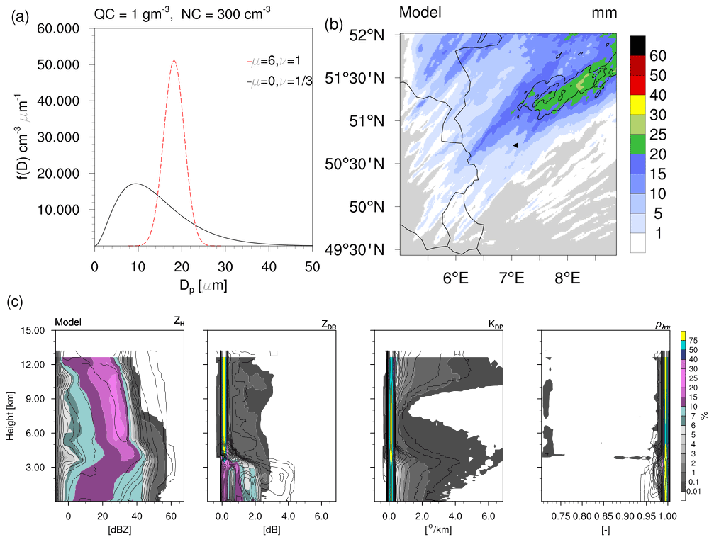
Figure 12(a) Modified gamma particle size distribution as a function of particle diameter (Dp) for the default and narrow cloud drop size distribution (CDSD). The bulk number concentration and mass density is 300 cm−3 and 1 gm−3, respectively. (b) Spatial pattern of ensemble-averaged accumulated precipitation for the default and narrow CDSD (solid contour lines with intervals at 20, 30 and 35 mm). (c) CFADs of horizontal reflectivity and differential reflectivity, specifically the differential phase and cross-correlation coefficient from 14:45 to 15:30 UTC on 5 July 2015. CFADs are shown for five ensemble members for narrow CDSD. The CFADs of the default experiment are shown in black contoured lines only.
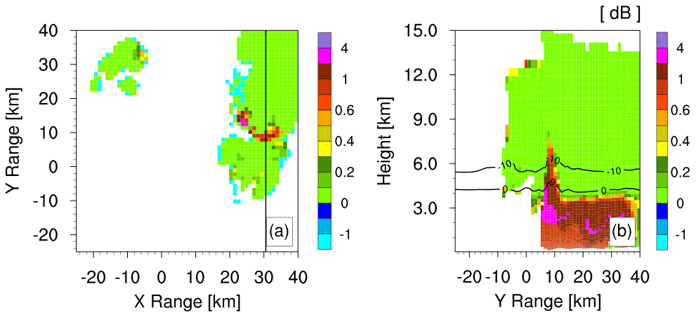
Figure 13Plan view (a) and vertical cross section (b) of differential reflectivity. The plan view is shown at 6 km height, and the cross section is passing through the solid line shown in the plan view. The 0 and −10 ∘C isotherm are also shown in the cross section.
In terms of observed polarimetric features, the synthetic polarimetric variables also exhibit ZDR-column-like feature (though of much weaker magnitude) along the updraft region, as in the observations. This difference may be attributed to a too small size of supercooled raindrops, but it may also be associated with the deficiency in the simulated updraft structure, recirculation of raindrops, and treatment of the slow freezing of raindrops (Kumjian et al., 2014; Snyder et al., 2015). Also, importantly, the ZDR signal contribution from water-coated hail owing to wet growth process is missing. The current FO only has a parameterization for the melting of hydrometeors, but the water-coated hail particles due to wet growth are not included. Furthermore, the collision efficiency between frozen particle and supercooled droplets decreases with drop size, resulting in a weaker riming and hence producing smaller hail particles with lower fall velocity (Noppel et al., 2010). The study by Noppel et al. (2010), using the COSMO model with SB2M microphysics, showed that the continental CN concentration led to a weaker hail storm; however, an additional sensitivity study, by varying the shape parameters for cloud droplets producing narrow distribution, led to a different conclusion, indicating the missing feedback between the shape parameters of cloud droplets and CN concentrations. So, we also conducted an additional ensemble sensitivity study using a narrow cloud droplet size distribution (CDSD; see Fig. 12a). The parameters μ and ν, determining the shape of the distribution, were changed to 6 and 1, respectively, from the default value used in this study and referred to as narrow CDSD. With the narrow CDSD runs, all ensemble members still underestimate the CAF. The change in CDSD led to a delay in the onset of CAF evolution, with some ensemble members exhibiting relatively higher CAF. However, the CAF time series exhibits different variability for each ensemble member, suggesting the strong influence of lateral boundary conditions. The domain average precipitation and the spread of the frequency distribution of the precipitation are similar to the default runs. Only the spatial location of high precipitation for the ensemble average in the northeastern part of the domain is slightly shifted (Fig. 12b). However, the narrow CDSD does show improvement in the simulated ZDR-column-like features, which is more well defined than the default experiment with larger mean raindrop size (0.5–1 mm) above the melting layer (Fig. 13). Besides, the narrow CDSD does affect the CFADs of the storm in terms of polarimetric variables (Fig. 12c). At upper levels, the peaks of ZH shift to higher magnitudes at 20 to 35 dbZ. And, the distribution gradually broadens, and the peak shifts rightward (30 to 40 dBZ) near the melting layer. Below the melting layer, the distribution shifts rightward, as simulated before (with default CDSD), with peaks around 5 to 25 dBZ. CFADs of ZDR also exhibit multimodal distribution below the melting layer with additional peaks around 0.87 and 1.87 dB, which is slightly lower than the default CDSD runs. Above the melting layer, the peak of ZDR remains at 0.11 dB. The CFADs of the KDP and ρHV also exhibit a similar peak around 0.11 ∘ km−1 and 0.99, respectively. But, in general, there is an increase in the spread of all the polarimetric variables. This could probably indicate the importance of the shape parameters of the hydrometeors for improving the simulated polarimetric signature of the storm.
While acknowledging the model biases and uncertainty in the simulated aerosol properties, the inclusion of prognostic aerosol is a way forward for a better understanding of the aerosol–cloud–precipitation interactions. During the convective storm event, the model generates aerosol-tower-like features with contrasting physical and chemical properties compared to the background.
At diurnal scales, the model is able to capture the spatial pattern of the precipitation; however, the comparison with the polarimetric observations indicates possible deviation in the ice hydrometeor partitioning above the melting layer (especially in the downdraft region of the storm), the size of supercooled raindrops and hail in the vicinity of the convective core, and the mechanism of rain production below the melting layer – hence the particle shapes and concentration. Constraining the CDSD did not produce any drastic difference in the simulated precipitation but produced an improvement in the simulated ZDR-column-like features. Thus, running simulations with prognostic aerosol and the use of a forward operator can also help to constrain the cloud droplet size distribution in the model. Besides the shortcomings in the traditional two-moment bulk scheme used in this study, the effect of the model grid resolution and its impact on the structure of the storm updraft and the effect of a simulated high number of aerosol concentration which is lifted in the convective core, and hence the polarimetric signature in the vicinity of the convective core, can also not be neglected.
Thus, future aerosol–cloud–precipitation interaction studies using models should make an effort to include prognostic aerosol models and evaluate the cloud microphysical processes using polarimetric radar data to identify and improve the cloud microphysical parameterization in the current numerical weather prediction model used for weather and climate prediction.
A1 Polarimetric radar data
The X-band Doppler radars are operating at a frequency of 9.3 GHz, with a radial resolution of 100–150 m and a scan period of 5 min. Both radars produce volume scans at different elevations, mostly between 0.5 and 30∘. These volume scans are also used to interpolate the polarimetric radar data from the native polar coordinates to Cartesian coordinates at 500 m horizontal and vertical resolution, using a Cressman analysis with a radius of influence of 2 km in the horizontal and 1 km in the vertical. A threshold of 0.8 in ρHV was imposed on the gridded data to ensure that clutter is filtered out without removing useful meteorological information.
The polarimetric variables ZH and ZDR are potentially affected by radar miscalibration, partial beam blockage, and (differential) attenuation, especially at smaller wavelengths (C band and X band), and their correction especially in deep convective, hail-bearing cells gives rise to additional uncertainties (e.g., Snyder et al., 2010; Shrestha et al., 2022). Although KDP estimates are not affected by miscalibration and attenuation, they can be substantially affected by the uncertainty in the quantification of the backscatter differential phase (δ), which is particularly important when hydrometeor sizes are in the range of, or larger than, the radar wavelength (Trömel et al., 2013). A more detailed discussion about the calibration, clutter filtering, and attenuation correction of the polarimetric radar data can be found in Shrestha et al. (2022). It is important to note that errors in the estimates of polarimetric radar variables might arise due to the assumptions made in the attenuation correction algorithm and due to uncertainties in the contribution of the backscatter differential phase to the total differential-phase shift. We acknowledge these limitations in the study and concentrate more on patterns and not so much on the actual magnitudes of the polarimetric moments.
A2 Trace gases and aerosols
NO2 is a key anthropogenic air pollutant and precursor of aerosols. The product comes with an estimated uncertainty for each VTC that could be used for the comparison between satellite and model. According to Boersma et al. (2011), Boersma et al. (2018), and Lamsal et al. (2021b), typical uncertainties are of the order of 30 % under clear-sky conditions. This should also hold for the data used in our study. The OMI estimates of VTC NO2 are filtered for data points with VcdfQualityFlags = 0 and CloudRadianceFraction < 0.5 (clear sky data). We did not include OMI HCHO and O3 for the following reasons: the HCHO product is extremely noisy. The retrieval uncertainty is 50 %–105 %, with the lower end being valid only for highly polluted locations. HCHO products are therefore usually only presented as monthly, seasonal, or yearly averages (e.g., De Smedt et al., 2021). The same argument holds for SO2. Comparing O3 would be quite interesting, but there is no official OMI tropospheric O3 product. Also, comparing the total column O3 from OMI would not be meaningful, as the column is strongly dominated by the stratosphere. Note also that, due to the long lifetime of O3, we would expect only very small gradients in the model domain.
A3 Polarimetric radar forward operator
For an offline run, EMVORADO requires as input the atmospheric fields of mass and (for SB2M) number concentrations of the six hydrometeor classes (cloud liquid, rain, cloud ice, snow, graupel, and hail) of temperature and of the three wind components. Other parameters that affect forward-modeled polarimetric radar observables are insufficiently constrained by the COSMO model, and assumptions need to be made within the FO. This regards, e.g., the phase partitioning of hydrometeors during melting, the shape and orientation of particles, and the heterogeneous microstructure of frozen hydrometeors.
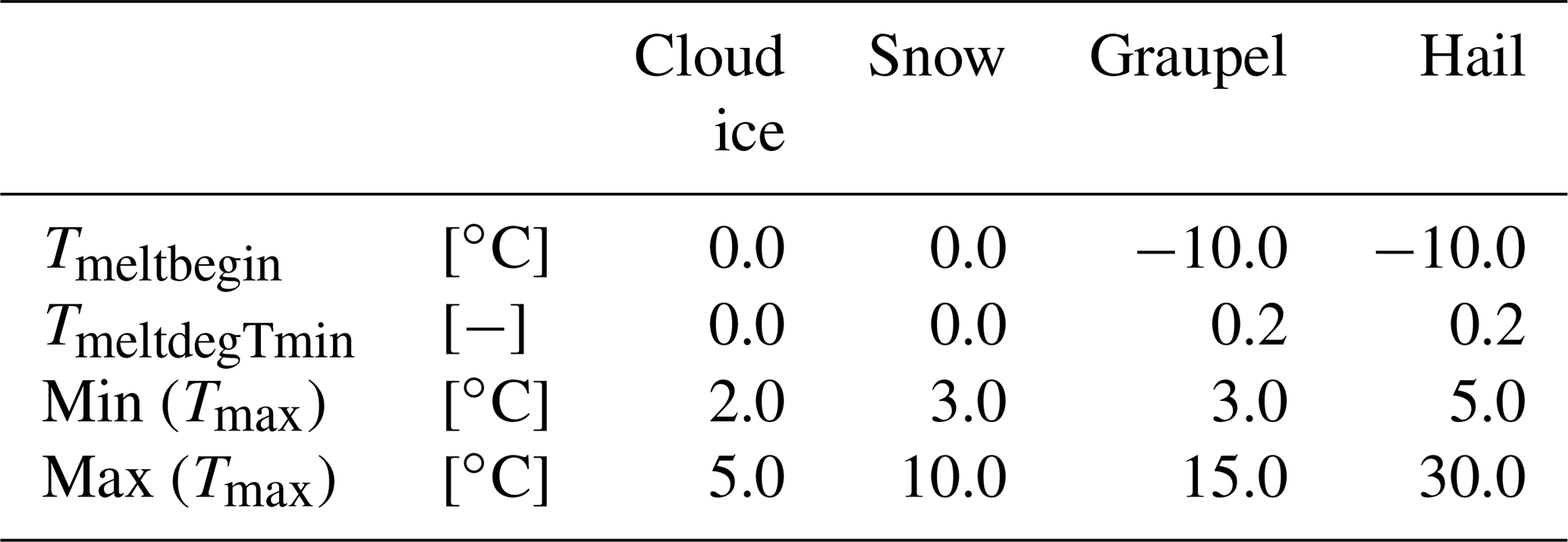
Like essentially all bulk scheme models, SB2M does not provide a prognostic melt fraction, and hydrometeors are either (completely) frozen or liquid. All meltwater is assumed to be shed instantaneously and transferred into the rain hydrometeor class; hence, no mixed-phase hydrometeors are predicted. Liquid water and ice exhibit significantly different dielectric properties in the radar frequency region, which leads to strong changes in the reflectivities where a phase change takes place. The melting layer is hence appearing very prominently in radar observations, particularly in stratiform situations, as layer of enhanced reflectivity known as the radar bright band. In order to be able to simulate such features, the forward operator needs to employ a melting scheme that predicts the occurrence of mixed-phase, wet frozen hydrometeors based on the single-phase model hydrometeors. EMVORADO employs a melting scheme that assumes a certain fraction of the frozen hydrometeor mass to be liquid (in contrast to, e.g., Wolfensberger and Berne, 2018, and Jung et al., 2008, who redistribute a part of the rainwater back into the frozen hydrometeor classes, i.e., unshed some rainwater). EMVORADO models the liquid water fraction dependent on the size of the hydrometeors (considering that small particles melt faster than large ones) and the ambient temperature T (Blahak, 2016). Wet hydrometeors start to occur when T exceeds a threshold Tmeltbegin and are assumed to be completely melted when Tmax is reached, where Tmax by default is determined dynamically from the model hydrometeor field and T in the vertical column. Setting Tmeltbegin accordingly allows for wet frozen hydrometeors at sub-zero temperatures, covering the case of the upward transport of liquid water and wet hydrometeors that do not (re-)freeze instantaneously in convective updrafts. Through the temperature dependence parameters, which are specific to each frozen hydrometeor class, the melting scheme can be adjusted by the user. Unless noted otherwise, in this study we apply EMVORADO's default melting scheme parameters (see Table A1).
Table A1Overview of EMVORADO melting scheme setup used in this study.
The shape and orientation of the hydrometeors significantly affect the polarimetric radar parameters but are entirely unconstrained by the COSMO model. Here we make use of the polarimetric mode of EMVORADO, which so far applies the T-matrix scattering method for one- (Mishchenko, 2000) or two-layered (Ryzhkov et al., 2011) spheroidal particles. All hydrometeors are assumed to be oblate spheroids (except for liquid cloud particles that are modeled as spheres using Rayleigh scattering) with hydrometeor class-specific and size- and melt-fraction-dependent parameterizations of shape and orientation of the hydrometeors, as given by Ryzhkov et al. (2011). The effect of orientation distributions is considered using the angular moments approach outlined in Ryzhkov (2001); Ryzhkov et al. (2011, 2013).
In order to allow the fast calculation of the radar observables, lookup tables of bulk scattering properties are pre-calculated, tabulating basic (additive) quantities per hydrometeor class over bulk (mean) mass, temperature, and melting Tmax. These are then added up over the six hydrometeor classes and converted into the polarimetric radar observables. Beside the reflectivity factor in horizontal polarization ZH, in this study we focus on the differential reflectivity ZDR, the co-polar cross-correlation coefficient ρHV, and the specific differential phase (KDP). In short, ZDR is the difference in the (log or dBZ space) reflectivities in the horizontal and vertical polarization, ρHV, the correlation between reflectivities in horizontal and vertical polarization within the measurement volume, and KDP the phase difference between the horizontal and vertical polarized wave returns. A more comprehensive description can be found, e.g., in Kumjian (2013).
EMVORADO is capable of simulating the sensing process, including scanning, beam tracing, beam blockage, beam pattern, attenuation. This allows us to directly simulate observation equivalents like 3D volume scans. However, here we make use of the radar parameters calculated on the model grid, i.e., neglecting any sensing effects. Further details about the FO and its sensitivity to assumed parameters for the hydrometeors can be found in Shrestha et al. (2022),Trömel et al. (2021), and Shrestha et al. (2022).
The source codes for TSMP and the setups used for this study are freely available from https://www.terrsysmp.org/ (Shrestha et al., 2014; Gasper et al., 2014) upon registration. The component models of TSMP have to be downloaded separately. The COSMO model is distributed to research institutions free of charge under an institutional license issued by the Consortium COSMO and administered by DWD. The radar forward operator EMVORADO is based on source code derived from the COSMO model; hence, redistribution is limited by the COSMO license. The ART v3.1 model can be obtained from https://www.imk-tro.kit.edu/english/5224.php (Vogel et al., 2009) by writing an email to bernhard.vogel@kit.edu.
The COSMO license also includes access to lateral boundary data provided by DWD. COSMO-DE EPS data used for the initial and lateral boundary conditions data for the COSMO model experiments in this study can be downloaded from the DWD database (https://www.dwd.de/DE/leistungen/pamore/pamore.html, DWD, 2022). The data used for soil–vegetation states are available at https://doi.org/10.5880/TR32DB.40 (Shrestha, 2021b). The CAMS-REG v4.2 data can be downloaded from https://doi.org/10.24380/eptm-kn40.
The Python package “emiproc” for emission pre-processing is available through the C2SM GitHub https://github.com/C2SM-RCM/cosmo-emission-processing (Jähn et al., 2020). The COSMO model Processing Chain version 2.2 is available from https://github.com/C2SM/processing-chain (EMPA, 2022). The source codes for the pre-processing and analysis of the model data, including scripts for plotting of figures, are available from GitHub (https://github.com/prabshr/prom, last access: 27 October 2022; https://doi.org/10.5281/zenodo.7246808, Shrestha, 2022).
PS conceptualized and designed the study, extended the TSMP modeling system with ART v3.1 and FO, conducted the model simulations and FO runs, carried out the analysis, and wrote the paper. JM made adaptations to the FO and aided in the model analysis and writing of the paper. DB contributed to the setup of the TSMP runs with ART v3.1 module and aided in the analysis of the model results and writing of the paper.
The contact author has declared that none of the authors has any competing interests.
Publisher’s note: Copernicus Publications remains neutral with regard to jurisdictional claims in published maps and institutional affiliations.
This article is part of the special issue “Fusion of radar polarimetry and numerical atmospheric modelling towards an improved understanding of cloud and precipitation processes (ACP/AMT/GMD inter-journal SI)”. It is not associated with a conference.
The research was carried out in the framework of the Priority Programme (grant no. SPP-451 2115) “Polarimetric Radar Observations meet Atmospheric Modelling (PROM)” funded by the German Research Foundation (DFG). Prabhakar Shrestha acknowledges support for the PROM sub-project ILACPR (grant no. SH 1326/1-1). Jana Mendrok carried out her work under the PROM sub-project Operation Hydrometeors (grant nos. BL 945/2-1). We gratefully acknowledge the computing time (grant no. terrsysmp-art) granted by the John von Neumann Institute for Computing (NIC) and provided on the supercomputer JUWELS at Jülich Supercomputing Centre (JSC). We would also like to thank Heike Vogel, for her support with the use of ART v3.1 module in COSMO. We also thank the Björn Nillius and Birger Bohn, for their effort in establishing and maintaining MAINZ and FJZ-JOYCE AERONET sites. The post-processing of model output data and input/output for FO was done using the NCAR Command Language (Version 6.4.0). Dust data and/or images were provided by the WMO Barcelona Dust Regional Center and the partners of the Sand and Dust Storm Warning Advisory and Assessment System (SDS-WAS) for northern Africa, the Middle East, and Europe.
This research has been supported by the Deutsche Forschungsgemeinschaft (grant no. SH 1326/1-1).
This paper was edited by Jianping Huang and reviewed by three anonymous referees.
Arino, O., Ramos Perez, J. J., Kalogirou, V., Bontemps, S., Defourny, P., and Van Bogaert, E.: Global Land Cover Map for 2009 (GlobCover 2009), © European Space Agency (ESA) & Université catholique de Louvain (UCL), PANGAEA [data set], https://doi.org/10.1594/PANGAEA.787668 2012. a
Ashby, S. F. and Falgout, R. D.: A parallel multigrid preconditioned conjugate gradient algorithm for groundwater flow simulations, Nucl. Sci. Eng., 124, 145–159, 1996. a
Baklanov, A., Schlünzen, K., Suppan, P., Baldasano, J., Brunner, D., Aksoyoglu, S., Carmichael, G., Douros, J., Flemming, J., Forkel, R., Galmarini, S., Gauss, M., Grell, G., Hirtl, M., Joffre, S., Jorba, O., Kaas, E., Kaasik, M., Kallos, G., Kong, X., Korsholm, U., Kurganskiy, A., Kushta, J., Lohmann, U., Mahura, A., Manders-Groot, A., Maurizi, A., Moussiopoulos, N., Rao, S. T., Savage, N., Seigneur, C., Sokhi, R. S., Solazzo, E., Solomos, S., Sørensen, B., Tsegas, G., Vignati, E., Vogel, B., and Zhang, Y.: Online coupled regional meteorology chemistry models in Europe: current status and prospects, Atmos. Chem. Phys., 14, 317–398, https://doi.org/10.5194/acp-14-317-2014, 2014. a
Baldauf, M., Seifert, A., Förstner, J., Majewski, D., Raschendorfer, M., and Reinhardt, T.: Operational convective-scale numerical weather prediction with the COSMO model: Description and sensitivities, Mon. Weather Rev., 139, 3887–3905, 2011. a
Bangert, M., Nenes, A., Vogel, B., Vogel, H., Barahona, D., Karydis, V. A., Kumar, P., Kottmeier, C., and Blahak, U.: Saharan dust event impacts on cloud formation and radiation over Western Europe, Atmos. Chem. Phys., 12, 4045–4063, https://doi.org/10.5194/acp-12-4045-2012, 2012. a, b, c, d
Barahona, D. and Nenes, A.: Parameterization of cloud droplet formation in large-scale models: Including effects of entrainment, J. Geophys. Res.-Atmos., 112, D16206, https://doi.org/10.1029/2007JD008473, 2007. a
Barahona, D. and Nenes, A.: Parameterizing the competition between homogeneous and heterogeneous freezing in cirrus cloud formation – monodisperse ice nuclei, Atmos. Chem. Phys., 9, 369–381, https://doi.org/10.5194/acp-9-369-2009, 2009. a
Barahona, D., West, R. E. L., Stier, P., Romakkaniemi, S., Kokkola, H., and Nenes, A.: Comprehensively accounting for the effect of giant CCN in cloud activation parameterizations, Atmos. Chem. Phys., 10, 2467–2473, https://doi.org/10.5194/acp-10-2467-2010, 2010. a
Barros, A. P. , Shrestha, P., Chavez, S., and Duan, Y.: Modeling Aerosol-Cloud-Precipitation Interactions in Mountainous Regions: Challenges in the Representation of Indirect Microphysical Effects with Impacts at Subregional Scales, in: Rainfall – Extremes, Distribution and Properties, edited by: Abbot, J. and Hammond, A., IntechOpen, https://doi.org/10.5772/intechopen.80025, 2018. a
Blahak, U.: Towards a better representation of high density ice particles in a state-of-the-art two-moment bulk microphysical scheme, in: Proc. 15th Int. Conf. Clouds and Precip., Cancun, Mexico, vol. 20208, 2008. a
Blahak, U.: RADAR_MIE_LM and RADAR_MIELIB - Calculation of Radar Reflectivity from Model Output, COSMO Technical Report 28, Consortium for Small Scale Modeling (COSMO), http://www.cosmo-model.org/content/model/cosmo/techReports/docs/techReport28.pdf (last access: 25 October 2022), 2016. a
Boersma, K. F., Eskes, H. J., Dirksen, R. J., van der A, R. J., Veefkind, J. P., Stammes, P., Huijnen, V., Kleipool, Q. L., Sneep, M., Claas, J., Leitão, J., Richter, A., Zhou, Y., and Brunner, D.: An improved tropospheric NO2 column retrieval algorithm for the Ozone Monitoring Instrument, Atmos. Meas. Tech., 4, 1905–1928, https://doi.org/10.5194/amt-4-1905-2011, 2011. a
Boersma, K. F., Eskes, H. J., Richter, A., De Smedt, I., Lorente, A., Beirle, S., van Geffen, J. H. G. M., Zara, M., Peters, E., Van Roozendael, M., Wagner, T., Maasakkers, J. D., van der A, R. J., Nightingale, J., De Rudder, A., Irie, H., Pinardi, G., Lambert, J.-C., and Compernolle, S. C.: Improving algorithms and uncertainty estimates for satellite NO2 retrievals: results from the quality assurance for the essential climate variables (QA4ECV) project, Atmos. Meas. Tech., 11, 6651–6678, https://doi.org/10.5194/amt-11-6651-2018, 2018. a
Craig, A., Valcke, S., and Coquart, L.: Development and performance of a new version of the OASIS coupler, OASIS3-MCT_3.0, Geosci. Model Dev., 10, 3297–3308, https://doi.org/10.5194/gmd-10-3297-2017, 2017. a
De Smedt, I., Pinardi, G., Vigouroux, C., Compernolle, S., Bais, A., Benavent, N., Boersma, F., Chan, K.-L., Donner, S., Eichmann, K.-U., Hedelt, P., Hendrick, F., Irie, H., Kumar, V., Lambert, J.-C., Langerock, B., Lerot, C., Liu, C., Loyola, D., Piters, A., Richter, A., Rivera Cárdenas, C., Romahn, F., Ryan, R. G., Sinha, V., Theys, N., Vlietinck, J., Wagner, T., Wang, T., Yu, H., and Van Roozendael, M.: Comparative assessment of TROPOMI and OMI formaldehyde observations and validation against MAX-DOAS network column measurements, Atmos. Chem. Phys., 21, 12561–12593, https://doi.org/10.5194/acp-21-12561-2021, 2021. a
Diederich, M., Ryzhkov, A., Simmer, C., Zhang, P., and Trömel, S.: Use of specific attenuation for rainfall measurement at X-band radar wavelengths. Part I: Radar calibration and partial beam blockage estimation, J. Hydrometeorol., 16, 487–502, 2015a. a
Diederich, M., Ryzhkov, A., Simmer, C., Zhang, P., and Trömel, S.: Use of specific attenuation for rainfall measurement at X-band radar wavelengths. Part II: Rainfall estimates and comparison with rain gauges, J. Hydrometeorol., 16, 503–516, 2015b. a
DWD (Deutscher Wetterdienst): Pamore – Abruf archivierter Daten der Vorhersagemodelle, DWD [data], https://www.dwd.de/DE/leistungen/pamore/pamore.html, last access: 22 October 2022. a
Emmons, L. K., Walters, S., Hess, P. G., Lamarque, J.-F., Pfister, G. G., Fillmore, D., Granier, C., Guenther, A., Kinnison, D., Laepple, T., Orlando, J., Tie, X., Tyndall, G., Wiedinmyer, C., Baughcum, S. L., and Kloster, S.: Description and evaluation of the Model for Ozone and Related chemical Tracers, version 4 (MOZART-4), Geosci. Model Dev., 3, 43–67, https://doi.org/10.5194/gmd-3-43-2010, 2010. a
EMPA: C2SM/processing-chain, EMPA [code], https://github.com/C2SM/processing-chain, last access: 25 October 2022. a
Fan, J., Leung, L. R., Rosenfeld, D., Chen, Q., Li, Z., Zhang, J., and Yan, H.: Microphysical effects determine macrophysical response for aerosol impacts on deep convective clouds, P. Natl. Acad. Sci. USA, 110, E4581–E4590, 2013. a
Fan, J., Wang, Y., Rosenfeld, D., and Liu, X.: Review of aerosol–cloud interactions: Mechanisms, significance, and challenges, J. Atmos. Sci., 73, 4221–4252, 2016. a
Fan, J., Rosenfeld, D., Zhang, Y., Giangrande, S. E., Li, Z., Machado, L. A., Martin, S. T., Yang, Y., Wang, J., Artaxo, P., Barbosa, H. M. J., Braga, R. C., Comstock, J. M., Feng, Z., Gao, W., Gomes, H. B., Mei, F., Pöhlker, C., Pöhlker, M. L., Pöschl, U., and Souza, R. A. F.: Substantial convection and precipitation enhancements by ultrafine aerosol particles, Science, 359, 411–418, 2018. a
Fountoukis, C. and Nenes, A.: Continued development of a cloud droplet formation parameterization for global climate models, J. Geophys. Res.-Atmos., 110, D11212, https://doi.org/10.1029/2004JD005591, 2005. a
Gasper, F., Goergen, K., Shrestha, P., Sulis, M., Rihani, J., Geimer, M., and Kollet, S.: Implementation and scaling of the fully coupled Terrestrial Systems Modeling Platform (TerrSysMP v1.0) in a massively parallel supercomputing environment – a case study on JUQUEEN (IBM Blue Gene/Q), Geosci. Model Dev., 7, 2531–2543, https://doi.org/10.5194/gmd-7-2531-2014, 2014 (data available at: https://www.terrsysmp.org/, last access: 27 October 2022). a, b
Gebhardt, C., Theis, S., Paulat, M., and Bouallègue, Z. B.: Uncertainties in COSMO-DE precipitation forecasts introduced by model perturbations and variation of lateral boundaries, Atmos. Res., 100, 168–177, 2011. a
Giles, D. M., Sinyuk, A., Sorokin, M. G., Schafer, J. S., Smirnov, A., Slutsker, I., Eck, T. F., Holben, B. N., Lewis, J. R., Campbell, J. R., Welton, E. J., Korkin, S. V., and Lyapustin, A. I.: Advancements in the Aerosol Robotic Network (AERONET) Version 3 database – automated near-real-time quality control algorithm with improved cloud screening for Sun photometer aerosol optical depth (AOD) measurements, Atmos. Meas. Tech., 12, 169–209, https://doi.org/10.5194/amt-12-169-2019, 2019. a, b
Guo, J., Deng, M., Lee, S. S., Wang, F., Li, Z., Zhai, P., Liu, H., Lv, W., Yao, W., and Li, X.: Delaying precipitation and lightning by air pollution over the Pearl River Delta. Part I: Observational analyses, J. Geophys. Res.-Atmos., 121, 6472–6488, 2016. a
Guo, J., Liu, H., Li, Z., Rosenfeld, D., Jiang, M., Xu, W., Jiang, J. H., He, J., Chen, D., Min, M., and Zhai, P.: Aerosol-induced changes in the vertical structure of precipitation: a perspective of TRMM precipitation radar, Atmos. Chem. Phys., 18, 13329–13343, https://doi.org/10.5194/acp-18-13329-2018, 2018. a
Holben, B. N., Eck, T. F., Slutsker, I. A., Tanre, D., Buis, J., Setzer, A., Vermote, E., Reagan, J. A., Kaufman, Y., Nakajima, T., Lavenu, F., Janakowiak, I., and Smirnov, A.: AERONET – A federated instrument network and data archive for aerosol characterization, Remote Sens. Environ., 66, 1–16, 1998. a
Igel, A. L. and van den Heever, S. C.: Invigoration or Enervation of Convective Clouds by Aerosols?, Geophys. Res. Lett., 48, e2021GL093804, https://doi.org/10.1029/2021GL093804, 2021. a
Iguchi, T., Rutledge, S. A., Tao, W.-K., Matsui, T., Dolan, B., Lang, S. E., and Barnum, J.: Impacts of aerosol and environmental conditions on maritime and continental deep convective systems using a bin microphysical model, J. Geophys. Res.-Atmos., 125, e2019JD030952, https://doi.org/10.1029/2019JD030952, 2020. a, b
Ilotoviz, E., Khain, A., Ryzhkov, A. V., and Snyder, J. C.: Relationship between aerosols, hail microphysics, and Z DR columns, J. Atmos. Sci., 75, 1755–1781, 2018. a
Jähn, M., Kuhlmann, G., Mu, Q., Haussaire, J.-M., Ochsner, D., Osterried, K., Clément, V., and Brunner, D.: An online emission module for atmospheric chemistry transport models: implementation in COSMO-GHG v5.6a and COSMO-ART v5.1-3.1, Geosci. Model Dev., 13, 2379–2392, https://doi.org/10.5194/gmd-13-2379-2020, 2020 (data available at: https://github.com/C2SM-RCM/cosmo-emission-processing, last access: 27 October 2022). a, b, c
Jiang, J. H., Su, H., Huang, L., Wang, Y., Massie, S., Zhao, B., Omar, A., and Wang, Z.: Contrasting effects on deep convective clouds by different types of aerosols, Nat. Commun., 9, 1–7, 2018. a
Jones, J. E. and Woodward, C. S.: Newton–Krylov-multigrid solvers for large-scale, highly heterogeneous, variably saturated flow problems, Adv. Water Resour., 24, 763–774, 2001. a
Jung, Y., Zhang, G., and Xue, M.: Assimilation of Simulated Polarimetric Radar Data for a Convective Storm Using the Ensemble Kalman Filter. Part I: Observation Operators for Reflectivity and Polarimetric Variables, Mon. Weather Rev., 136, 2228–2245, 2008. a
Khain, A., Rosenfeld, D., and Pokrovsky, A.: Aerosol impact on the dynamics and microphysics of deep convective clouds, Q. J. Roy. Meteor. Soc., 131, 2639–2663, 2005. a
Knote, C. and Brunner, D.: An advanced scheme for wet scavenging and liquid-phase chemistry in a regional online-coupled chemistry transport model, Atmos. Chem. Phys., 13, 1177–1192, https://doi.org/10.5194/acp-13-1177-2013, 2013. a
Knote, C., Brunner, D., Vogel, H., Allan, J., Asmi, A., Äijälä, M., Carbone, S., van der Gon, H. D., Jimenez, J. L., Kiendler-Scharr, A., Mohr, C., Poulain, L., Prévôt, A. S. H., Swietlicki, E., and Vogel, B.: Towards an online-coupled chemistry-climate model: evaluation of trace gases and aerosols in COSMO-ART, Geosci. Model Dev., 4, 1077–1102, https://doi.org/10.5194/gmd-4-1077-2011, 2011. a, b, c
Kollet, S. J. and Maxwell, R. M.: Integrated surface–groundwater flow modeling: A free-surface overland flow boundary condition in a parallel groundwater flow model, Adv. Water Resour., 29, 945–958, 2006. a
Koren, I., Martins, J. V., Remer, L. A., and Afargan, H.: Smoke invigoration versus inhibition of clouds over the Amazon, Science, 321, 946–949, 2008. a
Kreklow, J., Tetzlaff, B., Burkhard, B., and Kuhnt, G.: Radar-Based Precipitation Climatology in Germany – Developments, Uncertainties and Potentials, Atmosphere, 11, 217, https://doi.org/10.3390/atmos11020217, 2020. a
Krotkov, N. A., Lamsal, L. N., Marchenko, S. V., Bucsela, E. J., Swartz, W. H., Joiner, J., and the OMI core team: OMI/Aura Nitrogen Dioxide (NO2) Total and Tropospheric Column 1-orbit L2 Swath 13×24 km V003, 10.5067/aura/omi/data2017, Goddard Earth Sciences Data and Information Services Center (GES DISC) [data set], https://doi.org/10.5067/Aura/OMI/DATA2017, 2019. a
Kuenen, J. J. P., Visschedijk, A. J. H., Jozwicka, M., and Denier van der Gon, H. A. C.: TNO-MACC_II emission inventory; a multi-year (2003–2009) consistent high-resolution European emission inventory for air quality modelling, Atmos. Chem. Phys., 14, 10963–10976, https://doi.org/10.5194/acp-14-10963-2014, 2014. a
Kuenen, J., Dellaert, S., Visschedijk, A., Jalkanen, J.-P., Super, I., and Denier van der Gon, H.: Copernicus Atmosphere Monitoring Service regional emissions version 5.1 business-as-usual 2020 (CAMS-REG-v5.1 BAU 2020), Copernicus Atmosphere Monitoring Service, ECCAD [data set], https://doi.org/10.24380/eptm-kn40, 2021.
Kuenen, J., Dellaert, S., Visschedijk, A., Jalkanen, J.-P., Super, I., and Denier van der Gon, H.: CAMS-REG-v4: a state-of-the-art high-resolution European emission inventory for air quality modelling, Earth Syst. Sci. Data, 14, 491–515, https://doi.org/10.5194/essd-14-491-2022, 2022. a
Kulmala, M., Asmi, A., Lappalainen, H. K., Baltensperger, U., Brenguier, J.-L., Facchini, M. C., Hansson, H.-C., Hov, Ø., O'Dowd, C. D., Pöschl, U., Wiedensohler, A., Boers, R., Boucher, O., de Leeuw, G., Denier van der Gon, H. A. C., Feichter, J., Krejci, R., Laj, P., Lihavainen, H., Lohmann, U., McFiggans, G., Mentel, T., Pilinis, C., Riipinen, I., Schulz, M., Stohl, A., Swietlicki, E., Vignati, E., Alves, C., Amann, M., Ammann, M., Arabas, S., Artaxo, P., Baars, H., Beddows, D. C. S., Bergström, R., Beukes, J. P., Bilde, M., Burkhart, J. F., Canonaco, F., Clegg, S. L., Coe, H., Crumeyrolle, S., D'Anna, B., Decesari, S., Gilardoni, S., Fischer, M., Fjaeraa, A. M., Fountoukis, C., George, C., Gomes, L., Halloran, P., Hamburger, T., Harrison, R. M., Herrmann, H., Hoffmann, T., Hoose, C., Hu, M., Hyvärinen, A., Hõrrak, U., Iinuma, Y., Iversen, T., Josipovic, M., Kanakidou, M., Kiendler-Scharr, A., Kirkevåg, A., Kiss, G., Klimont, Z., Kolmonen, P., Komppula, M., Kristjánsson, J.-E., Laakso, L., Laaksonen, A., Labonnote, L., Lanz, V. A., Lehtinen, K. E. J., Rizzo, L. V., Makkonen, R., Manninen, H. E., McMeeking, G., Merikanto, J., Minikin, A., Mirme, S., Morgan, W. T., Nemitz, E., O'Donnell, D., Panwar, T. S., Pawlowska, H., Petzold, A., Pienaar, J. J., Pio, C., Plass-Duelmer, C., Prévôt, A. S. H., Pryor, S., Reddington, C. L., Roberts, G., Rosenfeld, D., Schwarz, J., Seland, Ø., Sellegri, K., Shen, X. J., Shiraiwa, M., Siebert, H., Sierau, B., Simpson, D., Sun, J. Y., Topping, D., Tunved, P., Vaattovaara, P., Vakkari, V., Veefkind, J. P., Visschedijk, A., Vuollekoski, H., Vuolo, R., Wehner, B., Wildt, J., Woodward, S., Worsnop, D. R., van Zadelhoff, G.-J., Zardini, A. A., Zhang, K., van Zyl, P. G., Kerminen, V.-M., S Carslaw, K., and Pandis, S. N.: General overview: European Integrated project on Aerosol Cloud Climate and Air Quality interactions (EUCAARI) – integrating aerosol research from nano to global scales, Atmos. Chem. Phys., 11, 13061–13143, https://doi.org/10.5194/acp-11-13061-2011, 2011. a
Kumar, P., Sokolik, I. N., and Nenes, A.: Parameterization of cloud droplet formation for global and regional models: including adsorption activation from insoluble CCN, Atmos. Chem. Phys., 9, 2517–2532, https://doi.org/10.5194/acp-9-2517-2009, 2009. a
Kumjian, M. R.: Principles and applications of dual-polarization weather radar. Part I: Description of the polarimetric radar variables, Journal of Operational Meteorology, 1, 226–242, https://doi.org/10.15191/nwajom.2013.0119, 2013. a, b
Kumjian, M. R. and Ryzhkov, A. V.: Polarimetric signatures in supercell thunderstorms, J. Appl. Meteorol. Clim., 47, 1940–1961, 2008. a
Kumjian, M. R., Khain, A. P., Benmoshe, N., Ilotoviz, E., Ryzhkov, A. V., and Phillips, V. T.: The anatomy and physics of Z DR columns: Investigating a polarimetric radar signature with a spectral bin microphysical model, J. Appl. Meteorol. Climatol., 53, 1820–1843, 2014. a, b, c
Lamsal, L. N., Krotkov, N. A., Vasilkov, A., Marchenko, S., Qin, W., Yang, E.-S., Fasnacht, Z., Joiner, J., Choi, S., Haffner, D., Swartz, W. H., Fisher, B., and Bucsela, E.: Ozone Monitoring Instrument (OMI) Aura nitrogen dioxide standard product version 4.0 with improved surface and cloud treatments, Atmos. Meas. Tech., 14, 455–479, https://doi.org/10.5194/amt-14-455-2021, 2021a. a
Lamsal, L. N., Krotkov, N. A., Vasilkov, A., Marchenko, S., Qin, W., Yang, E.-S., Fasnacht, Z., Joiner, J., Choi, S., Haffner, D., Swartz, W. H., Fisher, B., and Bucsela, E.: Ozone Monitoring Instrument (OMI) Aura nitrogen dioxide standard product version 4.0 with improved surface and cloud treatments, Atmos. Meas. Tech., 14, 455–479, https://doi.org/10.5194/amt-14-455-2021, 2021b. a
Lebo, Z. J. and Seinfeld, J. H.: Theoretical basis for convective invigoration due to increased aerosol concentration, Atmos. Chem. Phys., 11, 5407–5429, https://doi.org/10.5194/acp-11-5407-2011, 2011. a
Levy, R. and Hsu, C.: MODIS Atmosphere L2 Aerosol Product., 10.5067/modis/mod04_l2.061, NASA MODIS Adaptive Processing System, Goddard Space Flight Center [data set], USA, https://doi.org/10.5067/MODIS/MOD04_L2.061, 2015. a
Li, Z., Niu, F., Fan, J., Liu, Y., Rosenfeld, D., and Ding, Y.: Long-term impacts of aerosols on the vertical development of clouds and precipitation, Nat. Geosci., 4, 888–894, 2011. a
Löhnert, U., Schween, J. H., Acquistapace, C., Ebell, K., Maahn, M., Barrera-Verdejo, M., Hirsikko, A., Bohn, B., Knaps, A., O’Connor, E., Simmer, C., Wahner, A., and Crewell, S.: JOYCE: Jülich observatory for cloud evolution, B. Am. Meteorol. Soc., 96, 1157–1174, 2015. a
Majewski, D., Liermann, D., Prohl, P., Ritter, B., Buchhold, M., Hanisch, T., Paul, G., Wergen, W., and Baumgardner, J.: The operational global icosahedral–hexagonal gridpoint model GME: Description and high-resolution tests, Mon. Weather Rev., 130, 319–338, 2002. a
Martin, S. T., Andreae, M. O., Artaxo, P., Baumgardner, D., Chen, Q., Goldstein, A. H., Guenther, A., Heald, C. L., Mayol‐Bracero, O. L., McMurry, P. H., and Pauliquevis, T.: Sources and properties of Amazonian aerosol particles, Rev. Geophys., 48, RG2002, https://doi.org/10.1029/2008RG000280, 2010. a
Maxwell, R. M.: A terrain-following grid transform and preconditioner for parallel, large-scale, integrated hydrologic modeling, Adv. Water Resour., 53, 109–117, 2013. a
Milbrandt, J. A., Morrison, H., Dawson II, D. T., and Paukert, M.: A triple-moment representation of ice in the Predicted Particle Properties (P3) microphysics scheme, J. Atmos. Sci., 78, 439–458, 2021. a
Mishchenko, M. I.: Calculation of the amplitude matrix for a nonspherical particle in a fixed orientation, Appl. Opt., 39, 1026–1031, https://doi.org/10.1364/AO.39.001026, 2000. a
Morrison, H.: On the robustness of aerosol effects on an idealized supercell storm simulated with a cloud system-resolving model, Atmos. Chem. Phys., 12, 7689–7705, https://doi.org/10.5194/acp-12-7689-2012, 2012. a
Morrison, H. and Milbrandt, J. A.: Parameterization of cloud microphysics based on the prediction of bulk ice particle properties. Part I: Scheme description and idealized tests, J. Atmos. Sci., 72, 287–311, 2015. a
Noppel, H., Blahak, U., Seifert, A., and Beheng, K. D.: Simulations of a hailstorm and the impact of CCN using an advanced two-moment cloud microphysical scheme, Atmos. Res., 96, 286–301, 2010. a, b, c
Oleson, K. W., Niu, G. Y., Yang, Z. L., Lawrence, D. M., Thornton, P. E., Lawrence, P. J., Stöckli, R., Dickinson, R. E., Bonan, G. B., Levis, S., and Dai, A.: Improvements to the Community Land Model and their impact on the hydrological cycle, J. Geophys. Res.-Biogeo., 113, G01021, https://doi.org/10.1029/2007JG000563, 2008. a
Peralta, C., Ben Bouallègue, Z., Theis, S., Gebhardt, C., and Buchhold, M.: Accounting for initial condition uncertainties in COSMO-DE-EPS, J. Geophys. Res.-Atmos., 117, D07108, https://doi.org/10.1029/2011JD016581, 2012. a
Poll, S., Shrestha, P., and Simmer, C.: Modelling convectively induced secondary circulations in the terra incognita with TerrSysMP, Q. J. Roy. Meteor. Soc., 143, 2352–2361, 2017. a
Poll, S., Shrestha, P., and Simmer, C.: Grid resolution dependency of land surface heterogeneity effects on boundary-layer structure, Q. J. Roy. Meteor. Soc., 148, 141–158, 2022. a
Putaud, J. P., Van Dingenen, R., Alastuey, A., Bauer, H., Birmili, W., Cyrys, J., Flentje, H., Fuzzi, S., Gehrig, R., Hansson, H. C., and Harrison, R. M.: A European aerosol phenomenology–3: Physical and chemical characteristics of particulate matter from 60 rural, urban, and kerbside sites across Europe, Atmos. Environ., 44, 1308–1320, 2010. a
Ramsauer, T., Weiß, T., and Marzahn, P.: Comparison of the GPM IMERG final precipitation product to RADOLAN weather radar data over the topographically and climatically diverse Germany, Remote Sensing, 10, 2029, https://doi.org/10.3390/rs10122029, 2018. a
Rieger, D., Bangert, M., Kottmeier, C., Vogel, H., and Vogel, B.: Impact of aerosol on post-frontal convective clouds over Germany, Tellus B, 66, 22528, https://doi.org/10.3402/tellusb.v66.22528, 2014. a
Rosenfeld, D.: Suppression of rain and snow by urban and industrial air pollution, science, 287, 1793–1796, 2000. a
Rosenfeld, D., Lohmann, U., Raga, G. B., O'Dowd, C. D., Kulmala, M., Fuzzi, S., Reissell, A., and Andreae, M. O.: Flood or drought: how do aerosols affect precipitation?, Science, 321, 1309–1313, 2008. a
Rosenfeld, D., Andreae, M. O., Asmi, A., Chin, M., de Leeuw, G., Donovan, D. P., Kahn, R., Kinne, S., Kivekäs, N., Kulmala, M., and Lau, W.: Global observations of aerosol-cloud-precipitation-climate interactions, Rev. Geophys., 52, 750–808, 2014. a
Ryzhkov, A.: Interpretation of Polarimetric Radar Covariance Matrix for Meteorological Scatterers: Theoretical Analysis, J. Atmos. Ocean. Tech., 18, 315–328, https://doi.org/10.1175/1520-0426(2001)018<0315:IOPRCM>2.0.CO;2, 2001. a
Ryzhkov, A., Pinsky, M., Pokrovsky, A., and Khain, A.: Polarimetric Radar Observation Operator for a Cloud Model with Spectral Microphysics, J. Appl. Meteorol. Clim., 50, 873–894, https://doi.org/10.1175/2010JAMC2363.1, 2011. a, b, c
Ryzhkov, A. V. and Zrnic, D. S.: Polarimetric Characteristics of Deep Convective Storms, in: Radar Polarimetry for Weather Observations, 269–307, Springer, https://doi.org/10.1007/978-3-030-05093-1_8, 2019. a, b, c
Ryzhkov, A. V., Kumjian, M. R., Ganson, S. M., and Khain, A. P.: Polarimetric Radar Characteristics of Melting Hail. Part I: Theoretical Simulations Using Spectral Microphysical Modeling, J. Appl. Meteorol. Clim., 52, 2849–2870, https://doi.org/10.1175/JAMC-D-13-073.1, 2013. a
Seifert, A. and Beheng, K. D.: A two-moment cloud microphysics parameterization for mixed-phase clouds. Part 1: Model description, Meteorol. Atmos. Phys., 92, 45–66, 2006. a
Seifert, A., Köhler, C., and Beheng, K. D.: Aerosol-cloud-precipitation effects over Germany as simulated by a convective-scale numerical weather prediction model, Atmos. Chem. Phys., 12, 709–725, https://doi.org/10.5194/acp-12-709-2012, 2012. a
Shrestha, P.: Clouds and vegetation modulate shallow groundwater table depth, J. Hydrometeorol., 22, 753–763, 2021a. a, b
Shrestha, P.: High resolution hydrological simulations over Bonn Radar Domain, CRC/TR32 Database (TR32DB) [data set], https://doi.org/10.5880/TR32DB.40, 2021b. a
Shrestha, P.: Pre-processing and analysis of the TSMP-ART and polarimetric rdar data: v1.0 (v1.0), Zenodo [code], https://doi.org/10.5281/zenodo.7246808, 2022. a
Shrestha, P. and Barros, A. P.: Joint spatial variability of aerosol, clouds and rainfall in the Himalayas from satellite data, Atmos. Chem. Phys., 10, 8305–8317, https://doi.org/10.5194/acp-10-8305-2010, 2010. a
Shrestha, P., Barros, A. P., and Khlystov, A.: CCN estimates from bulk hygroscopic growth factors of ambient aerosols during the pre-monsoon season over Central Nepal, Atmos. Environ., 67, 120–129, 2013. a
Shrestha, P., Sulis, M., Masbou, M., Kollet, S., and Simmer, C.: A scale-consistent terrestrial systems modeling platform based on COSMO, CLM, and ParFlow, Mon. Weather Rev., 142, 3466–3483, 2014 (data available at: https://www.terrsysmp.org/, last access” 27 October 2022). a, b
Shrestha, P., Trömel, S., Evaristo, R., and Simmer, C.: Evaluation of modelled summertime convective storms using polarimetric radar observations, Atmos. Chem. Phys., 22, 7593–7618, https://doi.org/10.5194/acp-22-7593-2022, 2022. a, b, c, d, e, f, g, h, i
Shrestha, P., Mendrok, J., Pejcic, V., Trömel, S., Blahak, U., and Carlin, J. T.: Evaluation of the COSMO model (v5.1) in polarimetric radar space – impact of uncertainties in model microphysics, retrievals and forward operators, Geosci. Model Dev., 15, 291–313, https://doi.org/10.5194/gmd-15-291-2022, 2022. a
Snyder, J. C., Bluestein, H. B., Zhang, G., and Frasier, S. J.: Attenuation correction and hydrometeor classification of high-resolution, X-band, dual-polarized mobile radar measurements in severe convective storms, J. Atmos. Ocean. Tech., 27, 1979–2001, 2010. a
Snyder, J. C., Ryzhkov, A. V., Kumjian, M. R., Khain, A. P., and Picca, J.: A Z DR column detection algorithm to examine convective storm updrafts, Weather Forecast., 30, 1819–1844, 2015. a
Snyder, J. C., Bluestein, H. B., Dawson II, D. T., and Jung, Y.: Simulations of Polarimetric, X-Band Radar Signatures in Supercells. Part II: ZDR Columns and Rings and KDP Columns, J. Appl. Meteorol. Climatol., 56, 2001–2026, https://doi.org/10.1175/JAMC-D-16-0139.1, 2017b. a, b
Steppeler, J., Doms, G., Schättler, U., Bitzer, H., Gassmann, A., Damrath, U., and Gregoric, G.: Meso-gamma scale forecasts using the nonhydrostatic model LM, Meteorol. Atmos. Phys., 82, 75–96, 2003. a
Stevens, B. and Feingold, G.: Untangling aerosol effects on clouds and precipitation in a buffered system, Nature, 461, 607–613, 2009. a
Storer, R., Van den Heever, S., and L'Ecuyer, T.: Observations of aerosol-induced convective invigoration in the tropical east Atlantic, J. Geophys. Res.-Atmos., 119, 3963–3975, 2014. a
Storer, R. L., Van Den Heever, S. C., and Stephens, G. L.: Modeling aerosol impacts on convective storms in different environments, J. Atmos. Sci., 67, 3904–3915, 2010. a
Tao, W.-K., Li, X., Khain, A., Matsui, T., Lang, S., and Simpson, J.: Role of atmospheric aerosol concentration on deep convective precipitation: Cloud-resolving model simulations, J. Geophys. Res.-Atmos., 112, D24S18, https://doi.org/10.1029/2007JD008728, 2007. a
Tao, W.-K., Chen, J.-P., Li, Z., Wang, C., and Zhang, C.: Impact of aerosols on convective clouds and precipitation, Rev. Geophys., 50, RG2001, https://doi.org/10.1029/2011RG000369, 2012. a
Trömel, S., Kumjian, M. R., Ryzhkov, A. V., Simmer, C., and Diederich, M.: Backscatter differential phase—Estimation and variability, J. Appl. Meteorol. Clim., 52, 2529–2548, 2013. a
Trömel, S., Simmer, C., Blahak, U., Blanke, A., Doktorowski, S., Ewald, F., Frech, M., Gergely, M., Hagen, M., Janjic, T., Kalesse-Los, H., Kneifel, S., Knote, C., Mendrok, J., Moser, M., Köcher, G., Mühlbauer, K., Myagkov, A., Pejcic, V., Seifert, P., Shrestha, P., Teisseire, A., von Terzi, L., Tetoni, E., Vogl, T., Voigt, C., Zeng, Y., Zinner, T., and Quaas, J.: Overview: Fusion of radar polarimetry and numerical atmospheric modelling towards an improved understanding of cloud and precipitation processes, Atmos. Chem. Phys., 21, 17291–17314, https://doi.org/10.5194/acp-21-17291-2021, 2021. a, b, c
Vogel, B., Vogel, H., Bäumer, D., Bangert, M., Lundgren, K., Rinke, R., and Stanelle, T.: The comprehensive model system COSMO-ART – Radiative impact of aerosol on the state of the atmosphere on the regional scale, Atmos. Chem. Phys., 9, 8661–8680, https://doi.org/10.5194/acp-9-8661-2009, 2009 (data available at: https://www.imk-tro.kit.edu/english/5224.php, last access: 27 October 2022). a, b, c
Wolfensberger, D. and Berne, A.: From model to radar variables: a new forward polarimetric radar operator for COSMO, Atmos. Meas. Tech., 11, 3883–3916, https://doi.org/10.5194/amt-11-3883-2018, 2018. a
Yuan, T., Remer, L. A., Pickering, K. E., and Yu, H.: Observational evidence of aerosol enhancement of lightning activity and convective invigoration, Geophys. Res. Lett., 38, L04701, https://doi.org/10.1029/2010GL046052, 2011. a
Yuter, S. E. and Houze Jr., R. A.: Three-dimensional kinematic and microphysical evolution of Florida cumulonimbus. Part II: Frequency distributions of vertical velocity, reflectivity, and differential reflectivity, Mon. Weather Rev., 123, 1941–1963, 1995. a
Zeng, Y., Blahak, U., and Jerger, D.: An efficient modular volume-scanning radar forward operator for NWP models: description and coupling to the COSMO model, Q. J. Roy. Meteor. Soc., 142, 3234–3256, https://doi.org/10.1002/qj.2904, 2016. a
Zhang, Y., Fan, J., Li, Z., and Rosenfeld, D.: Impacts of cloud microphysics parameterizations on simulated aerosol–cloud interactions for deep convective clouds over Houston, Atmos. Chem. Phys., 21, 2363–2381, https://doi.org/10.5194/acp-21-2363-2021, 2021. a, b
- Abstract
- Introduction
- Data and methods
- Evaluation of simulated trace gases and aerosols
- Aerosol characterization
- Evaluation with polarimetric radar data
- Polarimetric feature and aerosol characteristics
- Discussion
- Conclusions
- Appendix A
- Code and data availability
- Author contributions
- Competing interests
- Disclaimer
- Special issue statement
- Acknowledgements
- Financial support
- Review statement
- References