the Creative Commons Attribution 4.0 License.
the Creative Commons Attribution 4.0 License.
 | 19 Oct 2022
An improved representation of aerosol mixing state for air quality–weather interactions
Robin Stevens
Andrei Ryjkov
Mahtab Majdzadeh
Ashu Dastoor
We implement a detailed representation of aerosol mixing state in the Global Environmental Multiscale – Modelling Air quality and CHemistry (GEM-MACH) air quality and weather forecast model. Our mixing-state representation includes three categories: one for more hygroscopic aerosol, one for less hygroscopic aerosol with a high black carbon (BC) mass fraction, and one for less hygroscopic aerosol with a low BC mass fraction. The more detailed representation allows us to better resolve two different aspects of aerosol mixing state: differences in hygroscopicity due to aerosol composition and the amount of absorption enhancement of BC due to non-absorbing coatings. Notably, this three-category representation allows us to account for BC thickly coated with primary organic matter, which enhances the absorption of the BC but has a low hygroscopicity.
We compare the results of the three-category representation (1L2B, (one hydrophilic, two hydrophobic)) with a simulation that uses two categories, split by hygroscopicity (HYGRO), and a simulation using the original size-resolved internally mixed assumption (SRIM). We perform a case study that is focused on North America during July 2016, when there were intense wildfires over northwestern North America. We find that the more detailed representation of the aerosol hygroscopicity in both 1L2B and HYGRO decreases wet deposition, which increases aerosol concentrations, particularly of less hygroscopic species. The concentration of PM2.5 increases by 23 % on average. We show that these increased aerosol concentrations increase cloud droplet number concentrations and cloud reflectivity in the model, decreasing surface temperatures.
Using two categories based on hygroscopicity yields only a modest benefit in resolving the coating thickness on black carbon, however. The 1L2B representation resolves BC with thinner coatings than the HYGRO simulation, resulting in absorption aerosol optical depths that are 3 % less on average, with greater differences over strong anthropogenic source regions. We did not find strong subsequent effects of this decreased absorption on meteorology.
- Article
(11856 KB) - Full-text XML
-
Supplement
(10688 KB) - BibTeX
- EndNote


Aerosol chemical mixing state refers to the distribution of chemical species across a population of aerosol particles. An aerosol population is said to be fully externally mixed if each aerosol particle consists of a single chemical species. If all chemical species are distributed evenly amongst all aerosol particles, then the aerosol population is said to be fully internally mixed. Aerosol populations in the real atmosphere are never fully externally mixed nor fully internally mixed but instead exist somewhere between these two extremes. In general, particles emitted from different sources are initially externally mixed with respect to each other and become more internally mixed with time through condensation, coagulation, and chemical reactions.
Internal mixing of hydrophilic and hydrophobic species can allow the hydrophobic species to act as cloud condensation nuclei (CCN) (e.g. McFiggans et al., 2006; Anttila, 2010; Kim et al., 2018; Dalirian et al., 2018). An increase in CCN concentrations will generally render clouds more reflective and can also increase cloud lifetime. Internal mixing of hydrophilic and hydrophobic species also allows the hydrophobic species to be more efficiently removed from the atmosphere through wet deposition. Additionally, weakly absorbing species can form a coating on black carbon (BC), which strongly absorbs solar radiation. The weakly absorbing species then act as a lens, enhancing the absorption of solar radiation by the BC, compared to the case where the BC is uncoated (e.g. Lesins et al., 2002; Liu and Mishchenko, 2018; Schnaiter et al., 2005; Cui et al., 2016). Estimates of the factor by which the absorption of BC increases due to coatings (the absorption enhancement) vary from 1 (no enhancement) to 4, with the majority of studies reporting values between 1 and 2.5 (Adachi et al., 2010; Zhang et al., 2008; Khalizov et al., 2009; Cappa et al., 2012; Lack et al., 2012; Liu et al., 2015; Peng et al., 2016; Schnaiter et al., 2005; Wang et al., 2014a; Xu et al., 2018; Zanatta et al., 2018; Y. Zhang et al., 2018). Differences in experimental methods and regional and seasonal variations in BC coating thickness both likely contribute to this diversity. This absorption enhancement leads to a local heating of the atmosphere and a cooling of the surface, potentially increasing stability and affecting cloud cover and precipitation (Bond et al., 2013; Boucher et al., 2013). We refer the reader to two recent reviews (Stevens and Dastoor, 2019; Riemer et al., 2019) for more details about aerosol mixing state.
Many previous representations of aerosol mixing state have been implemented in models to predict CCN concentrations and aerosol optical properties, and we include a partial list of these in Table 1. These include representing each particle individually (PartMC-MOSAIC; Riemer et al., 2009; Zaveri et al., 2010); multiple mixing-state categories separated by BC mass fraction, including MADRID-BC (Oshima et al., 2009b, a), ATRAS (Matsui et al., 2014; Matsui, 2017), MADE-soot (Riemer et al., 2003; Vogel et al., 2009), MADE-in (Aquila et al., 2011), and MADE-3 (Kaiser et al., 2019, 2014); two categories for at least BC and organic carbon based on hygroscopicity, implemented in GEOS-Chem (Bey et al., 2001; Wang et al., 2014b, 2018), the GLObal Model of Aerosol Processes (GLOMAP) in both its bin (Manktelow et al., 2010; Spracklen et al., 2005, 2011) and modal (Mann et al., 2010; Bellouin et al., 2013) configurations, GMXe (Pringle et al., 2010), the M3+ module (Wilson et al., 2001), M7 (Vignati et al., 2010; Stier et al., 2005; Vignati et al., 2004; Zhang et al., 2012), MAM4 (Liu et al., 2016), MAM7 (Liu et al., 2012), the Model for Ozone and Related chemical Tracers (MOZART; Emmons et al., 2010), and the Sectional Aerosol module for Large Scale Applications (SALSA; Bergman et al., 2012; Andersson et al., 2015; Kokkola et al., 2008; Tonttila et al., 2017; Kokkola et al., 2018); and representing all aerosol within the same size bin or mode as internally mixed, including the Canadian Aerosol Module (CanAM; Gong et al., 2006; Moran et al., 2012; Gong et al., 2003, 2015), CHIMERE (Menut et al., 2013), the Community Multiscale Air Quality (CMAQ, Binkowski and Roselle, 2003; Appel et al., 2013; Elleman and Covert, 2009; US EPA, 2017) model, the Modal Aerosol Dynamics module for Europe (MADE; Lauer et al., 2005), and the Modal Aerosol Module with three lognormal modes (MAM3; Liu et al., 2012). We refer the reader to Stevens and Dastoor (2019) for more detail on previous model representations of aerosol mixing state, including mixing-state representations that did not specifically target resolving CCN concentrations and optical properties, such as detailed categorizations based on chemical composition and source-oriented approaches. Previous studies using the model approaches listed above have found that if all aerosol in the same size bin or mode is assumed to be internally mixed, CCN concentrations will frequently be overestimated by 10 %–20 %, and absorption coefficients of BC will be overestimated by 20 %–40 % (Stevens and Dastoor, 2019, and references therein).
Riemer et al. (2009)Zaveri et al. (2010)Oshima et al. (2009a, b)Matsui et al. (2014)Matsui (2017)Riemer et al. (2003)Vogel et al. (2009)Aquila et al. (2011)Kaiser et al. (2019)Kaiser et al. (2014)Bey et al. (2001)Wang et al. (2018)Wang et al. (2014b)Manktelow et al. (2010)Spracklen et al. (2005)Spracklen et al. (2011)Mann et al. (2010)Bellouin et al. (2013)Pringle et al. (2010)Wilson et al. (2001)Vignati et al. (2010)Stier et al. (2005)Vignati et al. (2004)Zhang et al. (2012)Liu et al. (2016)Liu et al. (2012)Emmons et al. (2010)Bergman et al. (2012)Andersson et al. (2015)Kokkola et al. (2008)Tonttila et al. (2017)Kokkola et al. (2018)Gong et al. (2006)Moran et al. (2012)Gong et al. (2003, 2015)Menut et al. (2013)Binkowski and Roselle (2003)Appel et al. (2013)Elleman and Covert (2009)US EPA (2017)Lauer et al. (2005)Liu et al. (2012)Table 1Partial list of previous representations of mixing state in aerosol modules, from Stevens and Dastoor (2019). See text for expansion of acronyms, where applicable.

However, it still remains unclear as to how best to efficiently represent aerosol mixing state in atmospheric models. In this study, we implement a detailed representation of aerosol mixing state in the Global Environmental Multiscale – Modelling Air quality and CHemistry (GEM-MACH) (Moran et al., 2010) air quality model with online air quality–weather interactions. We refer to this new configuration of GEM-MACH as “GM-MixingState”. Our approach was inspired by the results of Ching et al. (2016): we independently account for both changes in hygroscopicity and BC mass fraction, as aerosol hygroscopic properties and optical properties do not necessarily co-vary. The existing air quality–weather interactions in GEM-MACH include aerosol–radiation interactions and changes in cloud droplet activation based on CCN concentrations (Gong et al., 2015; Majdzadeh et al., 2022). We perform a case study focused on biomass-burning over North America to evaluate GM-MixingState. We investigate the interactions between the representation of aerosol mixing state and air quality–weather interactions.
The paper is structured as follows: in Sect. 2, we describe the GEM-MACH model and the GM-MixingState configuration, as well as the experiments performed. In Sect. 3, we present our results and analysis. In Sect. 4, we summarize our study and present our conclusions.
GEM-MACH is an online chemical transport model embedded within the Environment and Climate Change Canada (ECCC) numerical weather prediction (NWP) model GEM (Côté et al., 1998a, b; Charron et al., 2012). GEM-MACH has been in use as the ECCC operational air quality prediction model since 2009 (Moran et al., 2010). The representations of many atmospheric processes in GEM-MACH are the same as in the ECCC AURAMS (A Unified Regional Air-quality Modelling System) offline chemical transport model (Gong et al., 2006), including gas-phase, aqueous-phase, and heterogeneous chemistry (inorganic gas–particle partitioning); secondary organic aerosol (SOA) formation; aerosol microphysics (nucleation, condensation, coagulation, and activation); sedimentation of particles; and dry deposition and wet removal (in-cloud and below-cloud scavenging) of gases and particles. The gas-phase and aqueous-phase chemistry mechanisms in GEM-MACH are adapted from ADOM (Acid Deposition and Oxidant Model; Venkatram et al., 1988; Fung et al., 1991). The heterogeneous chemistry mechanism currently implemented in GEM-MACH is a bulk scheme based on ISOROPPIA (Makar et al., 2003). Eight dry aerosol chemical species are included in GEM-MACH: sulfate, nitrate, ammonium, sea salt, dust and crustal material, SOA, primary organic aerosol (POA), and BC. We note that we will refer to dust and crustal material collectively as “dust” in the rest of this paper. GEM-MACH uses a single-moment aerosol scheme; it does not include a prognostic aerosol number tracer. When needed, diagnostic number concentrations are calculated assuming that aerosol particles within each size bin are monodisperse with a diameter equal to the midpoint diameter of the size bin.
By default, GEM-MACH uses a size-resolved internally mixed representation of the aerosol population: the aerosol population within each size bin is internally mixed, but the population of aerosol in each size bin is externally mixed with respect to each other size bin. The operational version of GEM-MACH uses two size bins (aerosol dry diameters 0–2.5 and 2.5–10 µm; Moran et al., 2010), but for this study we use 12 size bins spanning 10 nm to 10 µm. The 12 bin configuration has been shown to yield results that more closely resemble observations (Akingunola et al., 2018).
For this study, we implemented a more detailed representation of the aerosol mixing state into GEM-MACH. Within each size bin, we separate the aerosol into up to three mixing-state categories based on hygroscopicity and BC mass fraction: (1) high hygroscopicity (hi-κ); (2) low hygroscopicity, high BC mass fraction (lo-κ_hi-BC); and (3) low hygroscopicity, low BC mass fraction (lo-κ_lo-BC). This configuration is similar to the MADE-soot, MADE-in and MADE-3 aerosol modules, which include three categories: generally hydrophilic BC-free particles, hydrophilic BC-containing particles, and hydrophobic BC-containing particles. We differ in that we use a single category for all hydrophilic particles (hi-κ), and we use two categories for hydrophobic particles (lo-κ_hi-BC and lo-κ_lo-BC). This allows us to resolve BC coated with organic material (weakly hygroscopic but thickly coated) from BC that has thin coatings or no coatings of other aerosol matter (weakly hygroscopic and thinly coated). Each of the eight dry species are tracked in each mixing-state category, resulting in a total of 288 (8 species × 3 mixing-state categories × 12 size bins) aerosol tracers. Following the recommendations in Ching et al. (2016), we use a threshold value of the hygroscopicity parameter (κ; Petters and Kreidenweis, 2007) of 0.1 between hi-κ and lo-κ mixing-state categories and a threshold BC mass fraction of 0.3 between lo-BC and hi-BC mixing-state categories. We will discuss these mixing-state categories further in Sect. 2.2.
Coagulation of two particles within the same mixing-state category is assumed to result in a particle of the same mixing-state category, as both BC mass fraction and volume-weighted hygroscopicity would be within the range spanned by the two original particles. For coagulation of particles from two different mixing-state categories, we calculate the hygroscopicity and BC mass fraction of the new particle and add the mass to the mixing-state category that matches the new particle's properties. No other process directly transfers mass between mixing-state categories. However, after all other aerosol processes, we calculate the hygroscopicity and BC mass fraction for each size bin and mixing-state category. If either the hygroscopicity or the BC mass fraction is outside of the bounds of the current mixing-state category, all of the mass in the current combination of size bin and mixing-state category is moved to the mixing-state category that matches the hygroscopicity and BC mass fraction of the aerosol mass. Through this method, as condensation and other processes change the volume-weighted hygroscopicity and BC mass fraction over time, aerosol particles will generally move from the lo-κ_hi-BC mixing-state category to the lo-κ_lo-BC mixing-state category and from both lo-κ mixing-state categories to the hi-κ mixing-state category.
To calculate the hygroscopicity of aerosol in the model, we assume that sulfate, nitrate, ammonium, sea salt, dust, SOA, POA, and BC have κ values of 0.65, 0.65, 0.65, 1.1, 0.03, 0.1, 0.001, and 0, respectively (Ching et al., 2016; Zieger et al., 2017; Koehler et al., 2009). Following the volume Zdanovskii–Stokes–Robinson (ZSR) mixing rule (Petters and Kreidenweis, 2007), we assume that the hygroscopicity of a particle is the volume-weighted average of the component species. We therefore do not account explicitly for coating of insoluble components by soluble components, nor do we consider how particle size or shape may affect the mass fraction of coating material necessary for a particle to be rendered “hydrophilic”. However, other studies have shown that neither CCN concentrations (Liu et al., 2016; Lee et al., 2013) nor aerosol effective radiative forcing, either through aerosol–cloud interactions or through aerosol–radiation interactions (Regayre et al., 2018), are sensitive to the threshold amount of soluble material needed to render a particle hydrophilic. However, global burdens of BC and POA, especially in remote regions, have been shown to be sensitive to this parameter (Liu et al., 2012, 2016). This volume-weighted hygroscopicity is only used to determine the proper mixing-state category for aerosol. It is not used to determine cloud droplet activation.
Instead, cloud droplet activation is calculated using the parameterization for sectional models described by Abdul-Razzak and Ghan (2002). Particle hygroscopicity is calculated separately for each mixing-state category based on molecular weights and ion dissociation, as per Eq. (7) from Abdul-Razzak and Ghan (2002). Properties of SOA are assumed to be those of adipic acid; BC, POA and dust are assumed to be insoluble. We assume that aerosol in the lo-κ mixing-state categories does not participate in aqueous chemistry and is not removed by cloud-to-rain conversion and subsequent wet deposition. We discuss this in more detail in the Supplement. Aerosol in the lo-κ mixing-state categories is still removed from the atmosphere by below-cloud impaction by rain, as this process is not expected to depend strongly on aerosol composition.
Aerosol–radiation interactions are calculated as described in Majdzadeh et al. (2022). For the radiation calculations, sea spray and dust are always assumed to exist as pure particles, externally mixed from the other components. For each size bin within each mixing-state category, if the BC mass fraction is greater than 40 %, BC is also assumed to be externally mixed from other components. For each size bin within each mixing-state category, sulfate, nitrate, ammonium, and organic matter are assumed to be internally mixed. If the BC mass fraction is less than 40 %, we assume that these same species (sulfate, nitrate, ammonium, POA, and SOA) form a spherical shell over a spherical BC core in order to calculate an absorption enhancement factor. The total wet radius of the core-shell particle is calculated using the volume-weighted hygroscopic growth factor of the components in the core-shell particle. The absorption enhancement of the BC cores is then calculated following the parameterization of Bond et al. (2006) with the observationally constrained maximum threshold of 1.93 (Bond et al., 2006). However, we assume that there is no absorption enhancement for BC cores that comprise more than 40 % of the particle by mass, in agreement with more recent observations of thinly coated BC particles (Liu et al., 2017; Peng et al., 2016). This process is applied independently to each size bin and each mixing-state category.
We choose our domain and time period to be consistent with the 2016 North American domain used in the fourth phase of the Air Quality Model Evaluation International Initiative (AQMEII4; Galmarini et al., 2021). To reduce computational expenses while still providing sufficient data for analysis, we perform simulations only from 15 June to 31 July 2016, and we restrict our analysis to output from the month of July to provide sufficient time for spin-up. We use a 10 km horizontal resolution and 84 hybrid vertical levels up to 0.1 hPa, consistent with the ECCC contribution to AQMEII4 multi-model experiment. Chemical boundary conditions are sourced from a climatology from the global chemical transport model MOZART-4 (Model for Ozone and Related chemical Tracers, version 4; Emmons et al., 2010).
2.1 Emissions
The emissions inventories used in study are the same as those described in Majdzadeh et al. (2022) and very similar to the protocol for contributions to AQMEII4 (Galmarini et al., 2021). Anthropogenic emissions from Canada and the United States were sourced from the Canadian Air Pollutant Emissions Inventory and the US Environmental Protection Agency (EPA) 2011 Air Emissions Modelling Platform, respectively. We use forest fire emissions from the Canadian Forest Fire Emissions Production System (CFFEPS; Chen et al., 2019). The Sparse Matrix Operator Kernel Emissions (SMOKE) emissions processing system (https://www.cmascenter.org/smoke, last access: 15 July 2018; Bieser et al., 2011; Hogrefe et al., 2003; Houyoux et al., 2000) is used to speciate emissions prior to input within GEM-MACH (J. Zhang et al., 2018). Bulk aerosol mass emissions are associated with one of the 91 composite particulate matter speciation profiles compiled from the EPA's SPECIATE4.5 database (https://www.epa.gov/air-emissions-modeling/speciate-2, last access: 18 July 2018; Reff et al., 2009). Each composite particulate matter speciation profile gives relative fractions of sulfate, nitrate, ammonium, BC, and POA. Dust is defined to be the sum of all remaining species in the profile after these components are accounted for. Sea salt and SOA are assumed to make no contribution. As an example, particulate emissions from wildfires are speciated as 78.5 % POA, 9.7 % dust, 9.5 % BC, 1.3 % sulfate, 0.9 % ammonium, and 0.1 % nitrate. Sea-spray emissions are parameterized according to Gong (2003). GEM-MACH does not currently include natural dust emissions; the only natural dust included in our simulations is that included in the boundary conditions.
We differ from previous studies using GEM-MACH in that we allocate aerosol emissions across the different mixing-state categories, as follows: major stationary point-source emissions, such as emissions from smelters or fossil-fuel power plants, are assumed to be size-resolved internally mixed with other particulate mass from the same point source. Area emissions, including sea spray, dust, and disperse anthropogenic emissions, including traffic emissions, are assumed to be as close to fully externally mixed as possible within the limits of the mixing-state representation used. If all three mixing-state categories were used, sulfate, ammonium, nitrate, and sea spray would be emitted in the hi-κ category; dust and POA would be emitted into the lo-κ_lo-BC category; and BC would be emitted into the lo-κ_hi-BC category. There are no primary emissions of SOA. We note that these emissions are not truly fully externally mixed in reality and that this assumption will provide the maximum sensitivity to the mixing-state configuration used. However, observations have shown that particles emitted from traffic sources are either primarily BC or primarily organic, rather than being fully internally mixed at emission (Willis et al., 2016). Wildfire emissions are treated separately from other area emissions in GEM-MACH, and we assume that wildfire emissions are emitted into the lo-κ_lo-BC category, as BC-containing particles within wildfire emissions have been observed to frequently be thickly coated with low-hygroscopicity organic material (Perring et al., 2017; Kondo et al., 2011).
Table 2Temporally and spatially averaged results for each simulation.
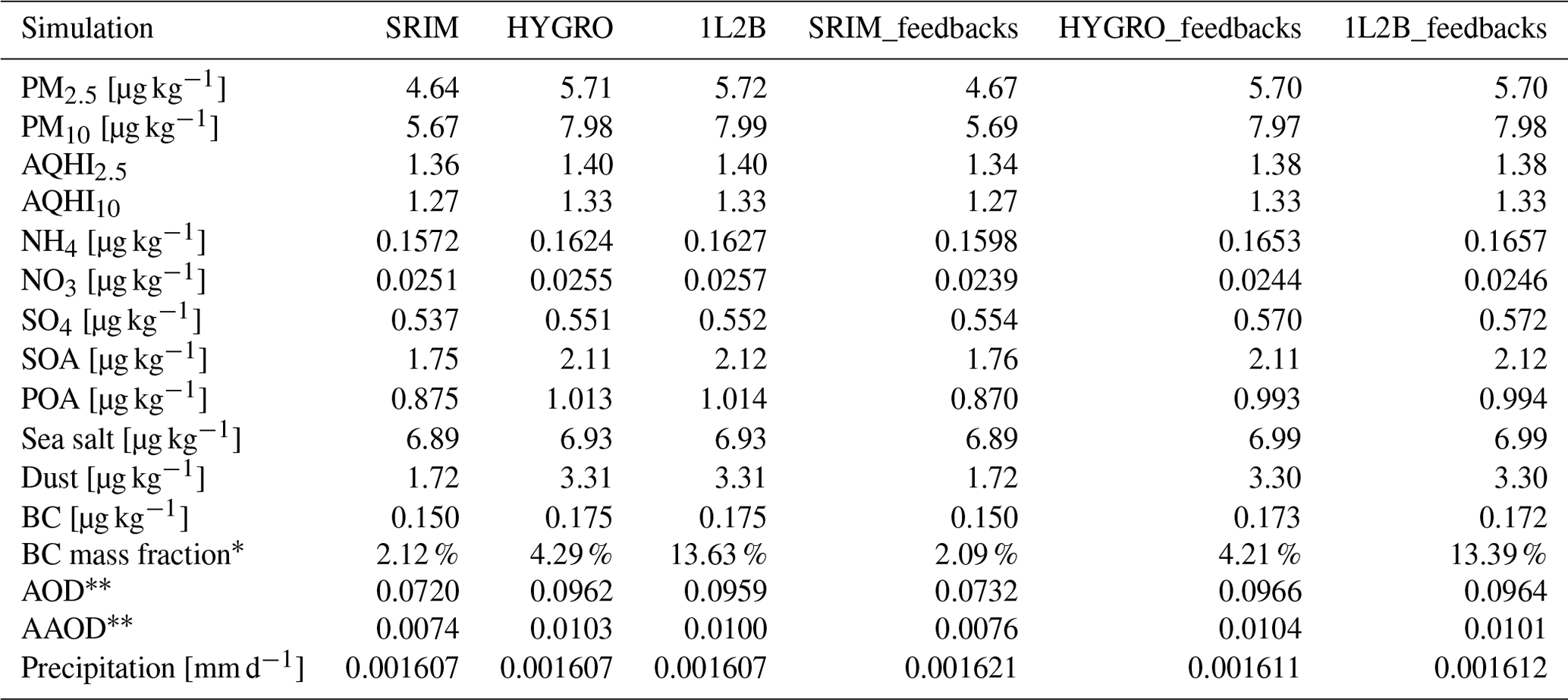
* Average BC mass fraction within BC-containing particles; see Sect. 3.1.4. Averaged over 13:00–21:00 UTC daily.
2.2 Sensitivity studies
An important question remains regarding the minimum level of complexity required to represent aerosol–weather feedbacks in air quality models well. We therefore perform several simulations with diverse representations of the aerosol mixing state. We consider a configuration with two mixing-state categories, split based on particle hygroscopicity (denoted as HYGRO representation; categories hi-κ and lo-κ). We also consider a mixing-state representation with three mixing-state categories: we use one mixing-state category for all high-hygroscopicity particles and two mixing-state categories for low-hygroscopicity particles, split based on BC mass fraction (high-κ, low-κ_hi-BC, and low-κ_lo-BC). We refer to this representation as 1L2B (one hydrophilic, two hydrophobic). We would not expect any improvement over HYGRO in the representation of the radiative properties of hydrophilic particles, but we would expect that 1L2B would better represent the radiative properties of low-hygroscopicity BC-containing particles. In particular, this representation should better distinguish BC thickly coated with POA from BC that is bare or only thinly coated with POA.
In addition to performing simulations with different representations of the aerosol mixing state, we also perform simulations with aerosol effects on meteorology (feedbacks) either permitted or disabled. When feedbacks are disabled, cloud droplet nucleation is independent of aerosol concentrations, and aerosol interactions with radiation have no effect on atmospheric temperatures or any other meteorological variables. Cloud droplet nucleation is instead determined following Cohard and Pinty (2010) as a function of updraft velocity, temperature, and pressure, assuming a pre-specified CCN concentration that does not vary with space or time. The meteorology in these simulations is independent of the aerosol and gas-phase concentrations. This allows us to directly attribute any differences in results solely to differences in aerosol processes caused by the differences in the representation of mixing state. We designate the simulations where aerosol effects on meteorology are permitted with the suffix “_feedbacks”, as these simulations include feedbacks of changes in aerosol concentrations and properties on the meteorology.
3.1 Non-feedback simulations
We present a summary of the domain-averaged, temporally averaged results from all simulations in Table 2. We will start by discussing differences between simulations with aerosol effects on weather disabled, in order to simplify the analysis. We remind the reader that because the meteorology is identical in these simulations, any differences in results can be attributed solely to differences in aerosol processes caused by the differences in the representation of mixing state.
3.1.1 Aerosol concentrations
We show the mean concentrations of particulate matter with a diameter smaller than 2.5 µm (PM2.5) in Fig. 1, along with the absolute and relative differences in PM2.5 concentrations between the HYGRO and size-resolved internally mixed (SRIM) simulations, and we show a similar figure for PM10 concentrations as Fig. S1. We note that PM2.5 and PM10 concentrations are very similar in the HYGRO and 1L2B simulations (Fig. S3). We find that spatially and temporally averaged surface PM2.5 concentrations and PM10 concentrations increase by 23 % and 41 %, respectively, from the SRIM simulation to either the HYGRO or 1L2B simulations. These differences are due mostly to increases in less hygroscopic species, with concentrations of BC, POA, SOA, and dust being increased in the HYGRO and 1L2B simulations by 16 %, 16 %, 21 %, and 93 %. The concentrations of more hygroscopic species (NH4, NO3, SO4, and sea-spray aerosol) were increased by 3 % or less.
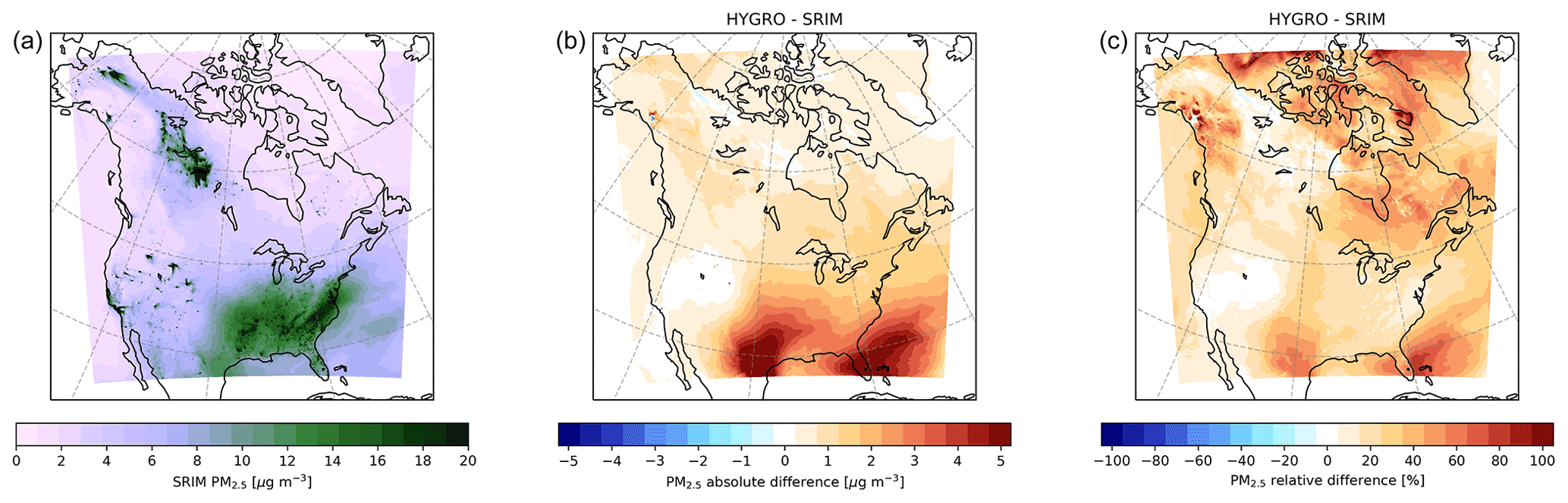
Figure 1(a) Mean PM2.5 concentrations from the SRIM simulation, (b) mean difference in PM2.5 concentrations between the HYGRO and SRIM simulations, and (c) relative difference in mean PM2.5 concentrations between the HYGRO and SRIM simulations.
These changes in aerosol concentrations are due primarily to changes in aerosol wet deposition. In the HYGRO and 1L2B simulations, all aerosol in the low-κ categories is excluded from in-cloud scavenging processes. However, direct comparison of wet deposition fluxes between simulations is complicated because of the greater aerosol mass concentrations in the HYGRO and 1L2B simulations than in the SRIM simulation. Even though the wet deposition process is less efficient for the same air parcel under the same conditions, local wet deposition fluxes can be greater in the HYGRO and 1L2B simulations due to the greater mass concentrations of aerosol in these simulations. For example, a reduced wet deposition flux close to an emissions source can yield an increased wet deposition flux further downwind, as more aerosol mass will be transported further downwind. We attempt to isolate for these effects by dividing the daily wet deposition flux by the daily mean surface aerosol concentrations, to approximate the wet deposition efficiency. This approach is limited in that cloud uptake of gases also contributes to the wet deposition fluxes, and cloud uptake of aerosol and subsequent wet deposition are not necessarily co-located in space and time with surface aerosol concentrations. However, we expect that the relationships between surface concentrations and wet deposition fluxes are similar enough across simulations for the comparison between simulations to be informative.
We show the temporal means of the wet deposition fluxes normalized by the surface aerosol concentrations in Fig. 2, along with the absolute and relative differences between the HYGRO and SRIM simulations. Both aerosol concentrations and wet deposition fluxes are very similar in the HYGRO and 1L2B simulations; therefore differences in normalized wet deposition between these simulations are also small (Fig. S4). We note that the normalized wet deposition shows some similar patterns to surface precipitation, as shown in Fig. 10, and the greatest values of normalized wet deposition are in the northern part of the domain where PM2.5 concentrations are low (Fig. 1). In the HYGRO simulation, normalized wet deposition fluxes decrease over most of the domain, except for some regions in the south of the model domain. Deeper clouds would be expected in this part of the domain, which may decouple wet deposition fluxes from surface aerosol concentrations. In the far north of the domain, there are large decreases in normalized wet deposition fluxes, in some cases approaching 100 %. These overlap with regions of low aerosol concentrations and large relative increases in surface aerosol concentrations, as shown in Fig. 1. However, other regions with greater mean surface aerosol concentrations and smaller differences in surface aerosol concentrations between the SRIM and HYGRO simulations also show large relative differences in normalized wet deposition fluxes. Normalized wet deposition fluxes over most of Canada are reduced by 20 %–80 %. A large part of this region is influenced by the forest fires that took place in Alaska and northern Canada during this period. As these forest fire emissions are composed primarily of POA, they are particularly sensitive to the changes in the representation of the aerosol mixing state.
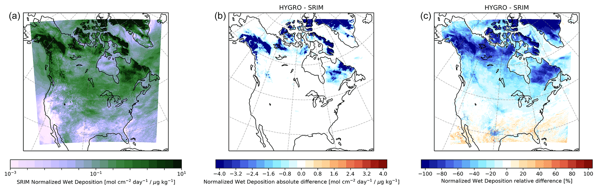
Figure 2(a) Temporal means of wet deposition fluxes normalized by surface total aerosol concentrations from the SRIM simulation, (b) mean difference in normalized wet deposition fluxes between the HYGRO and SRIM simulations, and (c) relative difference in mean normalized wet deposition fluxes between the HYGRO and SRIM simulations.
We can further control for differences in location and timing between wet deposition and surface concentrations by temporally and spatially averaging both the wet deposition fluxes and the surface concentrations before we divide the former by the latter. We therefore show the spatially and temporally averaged wet deposition fluxes normalized by the spatially and temporally averaged surface concentrations of each species in Table 3. After normalizing by the surface concentrations of aerosol, wet deposition rates of BC, POA, SOA, and dust were reduced in the HYGRO and 1L2B simulations by 27 %, 40 %, 12 %, and 10 %. The normalized wet deposition rates of more hygroscopic species were reduced by less than 5 %.
Table 3Temporally and spatially averaged wet deposition fluxes normalized by temporally and spatially averaged surface concentrations for each simulation. All units are mol cm−2 d−1 divided by µg kg−1.

In the HYGRO and 1L2B simulations, all aerosol in the low-κ categories is excluded from in-cloud scavenging processes. Since the low-κ category is defined as having a κ less than 0.1, this excludes large aerosol with low hygroscopicities from participating in in-cloud scavenging, even if their large size would allow them to activate as droplets despite their low hygroscopicity. In particular, this may cause the wet deposition of dust particles to be underestimated in the HYGRO and 1L2B simulations, while it is likely overestimated in the SRIM simulation. A more detailed treatment of cloud uptake of aerosol is beyond the scope of this study but will be revisited in a future version of GEM-MACH.
3.1.2 Comparison with observations
We compare the results of our non-feedback simulations against data from the Interagency Monitoring of Protected Visual Environments (IMPROVE; http://vista.cira.colostate.edu/Improve/, last access: 3 March 2022), the US EPA Chemical Speciation Network (CSN), and hourly measurements of PM2.5 and PM10 from the US EPA Air Quality System (AQS; https://www.epa.gov/aqs, last access: 3 March 2022). IMPROVE is a collaborative association of state, tribal, and federal agencies and international partners. US Environmental Protection Agency is the primary funding source, with contracting and research support from the National Park Service. The Air Quality Group at the University of California, Davis, is the central analytical laboratory, with ion analysis provided by Research Triangle Institute and carbon analysis provided by Desert Research Institute. We convert observed organic carbon to organic matter assuming a mass-to-carbon ratio of 1.8, consistent with the assumption routinely used to calculate aerosol extinction based on the IMPROVE data (Pitchford et al., 2007). We calculate a concentration of mineral dust as , and we calculate a concentration of sea salt as 3.25 Na for comparison to the model results.
We evaluate the SRIM and 1L2B simulations against the IMPROVE, CSN, and AQS data by calculating the correlation coefficient (R), the normalized mean bias (NMB), the root mean square error (RMSE), and the fraction of simulated data within a factor of 2 of the observations (Fac2), shown in Table 4. As noted previously, the concentrations of aerosol species in the HYGRO and 1L2B simulations are very similar. We note that R, NMB, and Fac2 differed by ≤ 0.03, and RMSE differed by < 0.01 µg m−3 between the SRIM and 1L2B results for sulfate, nitrate, and ammonium from the IMPROVE and CSN networks. The SRIM and 1L2B simulations therefore compare similarly well to observations for these species. This is expected, as these species are more weakly affected by the difference in mixing-state representation. There is an existing high bias in the SRIM-predicted concentrations of BC, organic aerosol, and dust. This high bias is worsened in the 1L2B simulation, due to the slower removal of these species by wet deposition in the 1L2B simulation, and this affects the calculated NMB, RMSE, and Fac2 values for these species. The correlation coefficients for elemental carbon (EC) and organic aerosol are not strongly affected. This suggests that the variability in BC and organic aerosol concentrations is not primarily controlled by wet deposition at these sites during the case study time period. As discussed, the wet deposition of dust is likely reduced too much in the 1L2B simulation, which may be responsible for the lower correlation between the observed and simulated dust concentrations in the 1L2B simulation. There is a slight shift of the sea salt size distribution to larger sizes in the 1L2B simulation, perhaps due to more coagulation with the larger concentrations of BC, organic aerosol, and dust. This reduces the fine sea salt aerosol mass, even while total sea salt aerosol concentrations slightly increase. The NMB and RMSE for sea salt are therefore reduced in the 1L2B simulation compared to the SRIM simulation. The increased concentrations of PM2.5 and PM10 in the 1L2B simulation increase the already high bias in PM2.5 and reduce the underprediction of PM10, as compared to the SRIM simulation. However, in both cases the RMSE is reduced, and the R and Fac2 values are either unchanged or slightly improved.
Table 4Evaluation of SRIM and 1L2B simulations against observations. N is the number of model–observation pairs, R is the correlation coefficient, NMB is the normalized mean bias, RMSE is the root mean square error, and Fac2 is the fraction within a factor of 2. Better performance between SRIM and 1L2B (larger values of R and Fac2 and smaller values of NMB and RMSE) is shown in bold font.

3.1.3 Air Quality Health Index
The Air Quality Health Index (AQHI; Stieb et al., 2008) is used by Environment and Climate Change Canada to communicate adverse health risks due to poor air quality to Canadians. It is formulated as a scale that ranges from 0 (excellent air quality) to 10 (very poor air quality) and is calculated based on the concentrations of PM2.5 or PM10, ozone (O3), and nitrogen dioxide (NO2). While the equations for calculating the AQHI permit values greater than 10 under exceptionally high concentrations of PM2.5, PM10, O3, or NO2, we restrict the values of AQHI to a maximum of 10, both because this is the intended range of the AQHI and to reduce the influence of exceptional, highly concentrated plumes in uninhabited areas (such as those from forest fires) on our results.
The concentration of O3 was, on average, 0.05 % less in the HYGRO or 1L2B cases than the SRIM case, and the concentration of NO2 was, on average, 0.2 % greater in the HYGRO or 1L2B cases than the SRIM case. We can therefore attribute differences in the AQHI primarily to differences in PM2.5 and PM10. The PM2.5 AQHI values in the HYGRO and 1L2B cases were nearly identical; the differences between them are shown in Fig. S5. The PM2.5 AQHI was, on average, 0.04 units greater in the HYGRO and 1L2B simulations than in the SRIM simulation, and the PM10 AQHI was 0.06 units greater in the HYGRO and 1L2B simulations than in the SRIM simulation. This can be seen in the spatial patterns of the differences in AQHI, shown in Fig. 3 for PM2.5 AQHI and in Fig. S2 for PM10 AQHI.
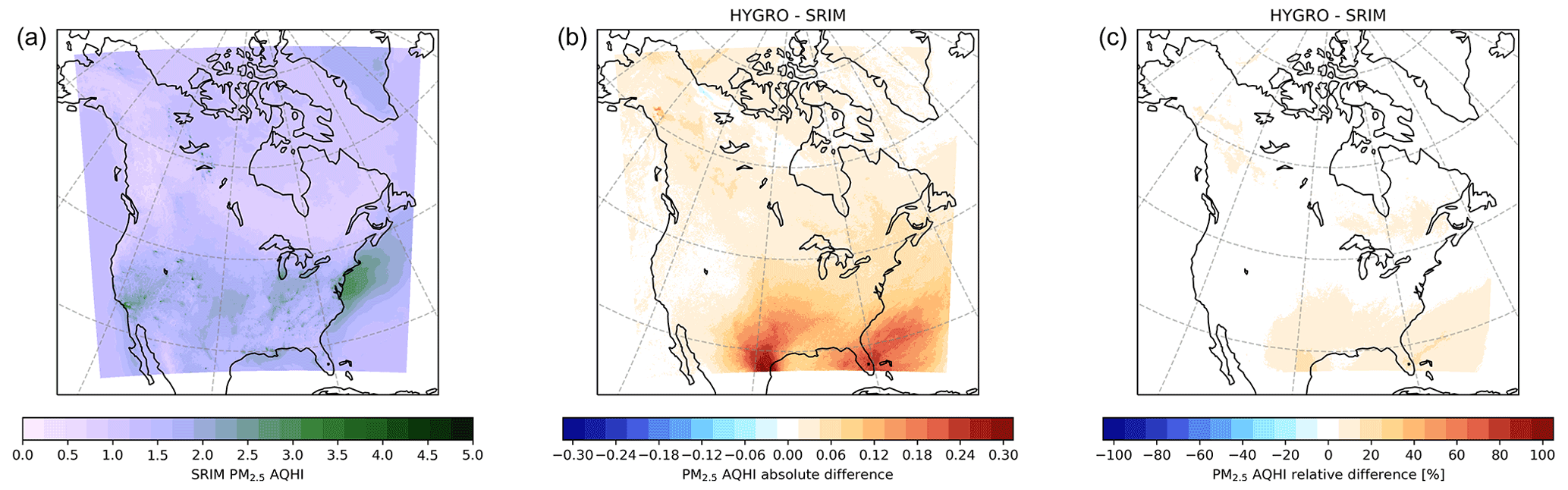
Figure 3(a) Mean PM2.5 AQHI values from the SRIM simulation, (b) mean difference in PM2.5 AQHI values between the HYGRO and SRIM simulations, and (c) relative difference in mean PM2.5 AQHI values between the HYGRO and SRIM simulations. Note that PM2.5 AQHI values are nearly identical in the HYGRO and 1L2B simulations.
3.1.4 BC mass fraction in BC-containing particles
Before discussing the BC mass fractions, we will discuss the concentrations of BC in more detail. We show in Fig. 4 the mean BC mixing ratios at the surface from the SRIM simulation, as well as the absolute and relative differences in the BC mixing ratio between the HYGRO and SRIM simulations. The BC mixing ratios in the HYGRO and 1L2B simulations were very similar; the differences are shown in Fig. S6. We note that during the time period simulated, several large forest fires burned in Alaska and northern Canada (see BC emissions in Fig. S9), and the influence of these fires on PM2.5, AQHI2.5, and BC mixing ratios is clearly visible in Figs. 1, 3, and 4, respectively.

Figure 4(a) Mean surface BC mixing ratios from the SRIM simulation, (b) mean difference in BC mixing ratios between the HYGRO and SRIM simulations, and (c) relative difference in mean BC mixing ratios between the HYGRO and SRIM simulations.
As discussed in Sect. 3.1.1, the mixing ratios of BC typically increase in the HYGRO and 1L2B simulations, as less BC is removed through wet deposition. However, there are notable locations downwind of forest fires in Alaska and northern Canada where the mixing ratios of BC at the surface decrease. If we examine the differences in BC concentrations at a higher altitude typically above clouds, as shown at about 185 hPa above the surface in Fig. S7, we do not see these decreases, but we do see that BC from these wildfires has been lofted to this altitude. Aerosol in the high-κ category and all aerosol in the SRIM simulation that is sufficiently large can be ingested into cloud droplets. These cloud droplets can grow to drizzle sizes and would then be subject to gravitational settling. If the drizzle droplets evaporate before reaching the surface, they will transport any aerosol mass in the droplets to lower altitudes. However, aerosol in the low-κ categories in the HYGRO and 1L2B simulations is not subject to this process, and therefore BC that is lofted to higher altitudes takes longer to reach the surface in these simulations, reducing the surface mixing ratios close to the forest fires and increasing them further downwind. For this reason, the peaks in absolute differences are further downwind at the surface, in Ontario and Quebec (Fig. 4), than at about 185 hPa above the surface, where the peaks in absolute differences are in Nunavut and above Hudson's Bay (Fig. S7).
In order to explain the effects of the mixing-state representation on aerosol–radiation interactions (discussed further in Sect. 3.1.5), we calculate the BC mass fraction within particles that contain BC. To do this, we calculate the BC mass fraction in each combination of size bin and mixing-state category separately and then report the average value weighted by the mass of BC in the same combination of size bin and mixing-state category. We show these results in Fig. 5. The SRIM configuration assumes that BC is internally mixed with all other aerosol mass in particles of the same size; thus the BC mass fraction is similar to the total BC mass divided by the total aerosol mass. For 99 % of the grid cells, the mean BC mass fraction in the SRIM simulation is less than 5 %. The HYGRO configuration shows modest improvements over the SRIM configuration, while the 1L2B configuration is able to resolve many regions close to emission sources where BC is thinly coated (high BC mass fractions). The high spatial resolution of GEM-MACH is an asset in resolving these regions close to emission sources.
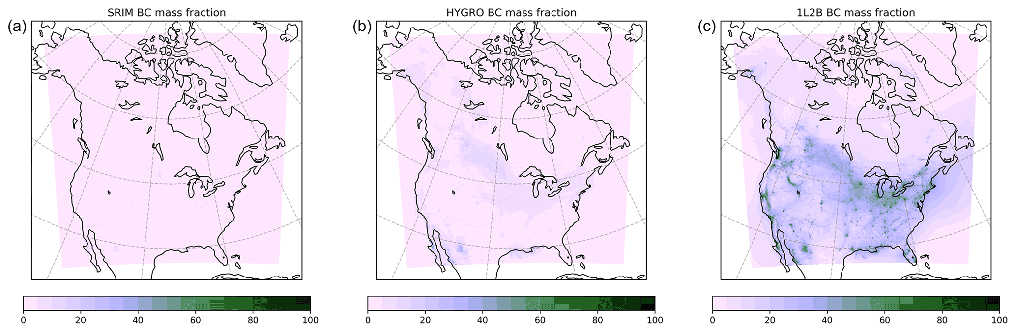
Figure 5Black carbon mass fractions in BC-containing particles. Values are given at the surface and weighted by the BC mass in each size bin and mixing-state category. Values are shown for the following simulations: (a) SRIM, (b) HYGRO, and (c) 1L2B.
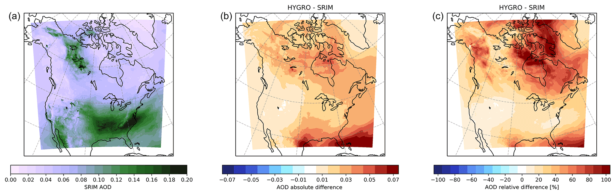
Figure 6(a) Mean AOD from the SRIM simulation, (b) mean difference in AOD between the HYGRO and SRIM simulations, and (c) relative difference in mean AOD between the HYGRO and SRIM simulations. Only results from the hours of 13:00–21:00 UTC are included as the AOD is only calculated during local daylight hours.
We note that the 1L2B simulation is better able to capture regions with large BC mass fractions than the HYGRO simulation because the HYGRO configuration assumes that all low-hygroscopicity species within the same size bin are internally mixed, including BC, dust, and POA. Most dust mass exists in larger size bins than BC. Therefore, even the SRIM simulation does not assume much internal mixing of BC and dust. However, BC and POA are emitted into the same size bins and from the same source regions. When the BC is assumed to be internally mixed with other low-hygroscopicity species, the resulting particles frequently consist of BC thickly coated with POA. The 1L2B simulation is able to distinguish BC thinly coated with POA from BC thickly coated with POA, and it predicts that a large proportion of BC near source regions only has a thin coating of non-BC species.
3.1.5 Aerosol–radiation interactions
We show the monthly mean AOD from the SRIM simulation and the difference between the HYGRO and SRIM simulations in Fig. 6. We remind the reader that the calculations of aerosol optical properties are restricted to daylight hours in GEM-MACH. As such, we only include data from between 13:00 and 21:00 UTC in Fig. 6, in order to exclude times of day when the AOD was not calculated for some part of the domain shown. We also note that the mean AOD in the 1L2B and HYGRO simulations differs by no more than 0.9 % for any grid cell in the domain, as shown in Fig. S8. When using the HYGRO configuration, the AOD is 34 % larger than in the SRIM case. A comparison of the AOD with the absorption aerosol optical depth (AAOD) (see Table 2 and Fig. 7) reveals that the AOD is dominated by aerosol scattering, rather than aerosol absorption. Previous studies have found that the optical properties of non-absorbing aerosol are not strongly sensitive to the mixing state of the aerosol (e.g. Zaveri et al., 2010; Klingmüller et al., 2014) and that because AOD is dominated by the scattering component, ambient AOD is not strongly sensitive to mixing state (e.g. Matsui et al., 2013, 2014; Klingmüller et al., 2014; Han et al., 2013), although a recent study has shown that aerosol scattering can be very sensitive to aerosol mixing state under certain conditions (Yao et al., 2022). We therefore do not expect our more detailed representation of the BC mass to yield strong changes in aerosol scattering, but we do expect a decrease in aerosol absorption. We therefore conclude that the differences are due predominantly to the increases in aerosol mass, in turn due to the decrease in aerosol wet deposition. This is supported by the fact that the aerosol AOD and differences in AOD are visibly well correlated with PM2.5 and the differences in PM2.5 shown in Fig. 1.
We show the monthly mean AAOD from the SRIM simulation and the differences between the 1L2B, HYGRO, and SRIM simulations in Fig. 7. The AAOD is 39 % higher in the HYGRO case than in the SRIM case. As shown in Fig. 5, the BC mass fraction in BC-containing particles is only slightly larger in the HYGRO case than the SRIM cases. If the mass concentrations of all aerosol species were equal in both cases, higher BC mass fractions would imply thinner coatings and smaller absorption enhancements for the BC-containing particles. This effect would be expected to reduce the AAOD in the HYGRO case as compared to the SRIM case. The simulated increase in AAOD is due primarily to the increased concentrations of BC in the HYGRO case compared to the SRIM case.

Figure 7(a) Mean AAOD from the SRIM simulation, (b) mean difference in AAOD between the HYGRO and SRIM simulations, (c) relative difference in mean AAOD between the HYGRO and SRIM simulations, (d) mean difference in AAOD between the 1L2B and HYGRO simulations, and (e) relative difference in mean AAOD between the 1L2B and HYGRO simulations. Only results from the hours of 13:00–21:00 UTC are included as the AOD is only calculated during local daylight hours.
When using the 1L2B configuration, the AAOD is on average 3 % less than in the HYGRO case, with these decreases being primarily over the eastern United States and around the Gulf of California. These are similar to the regions where the 1L2B case has higher BC mass fractions than the HYGRO case, as shown in Fig. 5, and are typically downwind of large anthropogenic sources of BC. We note that there are smaller differences in the plumes of the large northern forest fires; this is because emissions of BC from forest fires are assumed to be thickly coated as observations (Perring et al., 2017; Kondo et al., 2011) have shown that this is typically the case. Around the Gulf of California and just south the Great Lakes region, the decreases in AAOD between 1L2B and HYGRO (due to better-resolving the coating thickness on BC) are larger in magnitude than the increases in AAOD between HYGRO and SRIM (due to reduced wet deposition of low-hygroscopicity aerosol, including BC). As seen in Fig. 2, wet deposition was relatively low during our simulations in both of these regions, especially around the Gulf of California. This is due largely to less cloudiness and to less precipitation, which is shown in Fig. 10. Also, both of these regions have greater emissions of anthropogenic BC, as can be seen in Fig. S9. Therefore in these regions, there is a net decrease in AAOD from the SRIM to 1L2B, when both the effects of mixing state on wet deposition and absorption enhancement are considered, while for most of the rest of the North American domain, AAOD increases as the effect due to decreases in wet deposition is more important than the effect due to decreased absorption enhancement.
3.2 Aerosol–meteorology feedbacks
In order to examine the interactions between aerosol mixing-state representation and meteorology, we will now describe the results of the aerosol–meteorology feedback simulations. In these simulations, the cloud droplet number concentration is parameterized based on the aerosol size distribution using Abdul-Razzak and Ghan (2002), as described in Sect. 2 and the Supplement. In the case of multiple mixing-state categories, the distinct composition of aerosol in each mixing-state category is considered, so aerosol in different mixing-state categories will have different critical radii for activation under the same atmospheric conditions. Additionally, aerosol and trace gas concentrations are permitted to reduce incoming radiation, which would subsequently alter atmospheric and surface energy balances.
As our focus is on the effects of differences in the aerosol mixing-state representation, we only compare cases with aerosol–meteorology feedbacks to other cases with aerosol–meteorology feedbacks. For comparisons of GEM-MACH results with and without aerosol–meteorology feedbacks, we refer the reader to Gong et al. (2015) and Makar et al. (2015a, b).
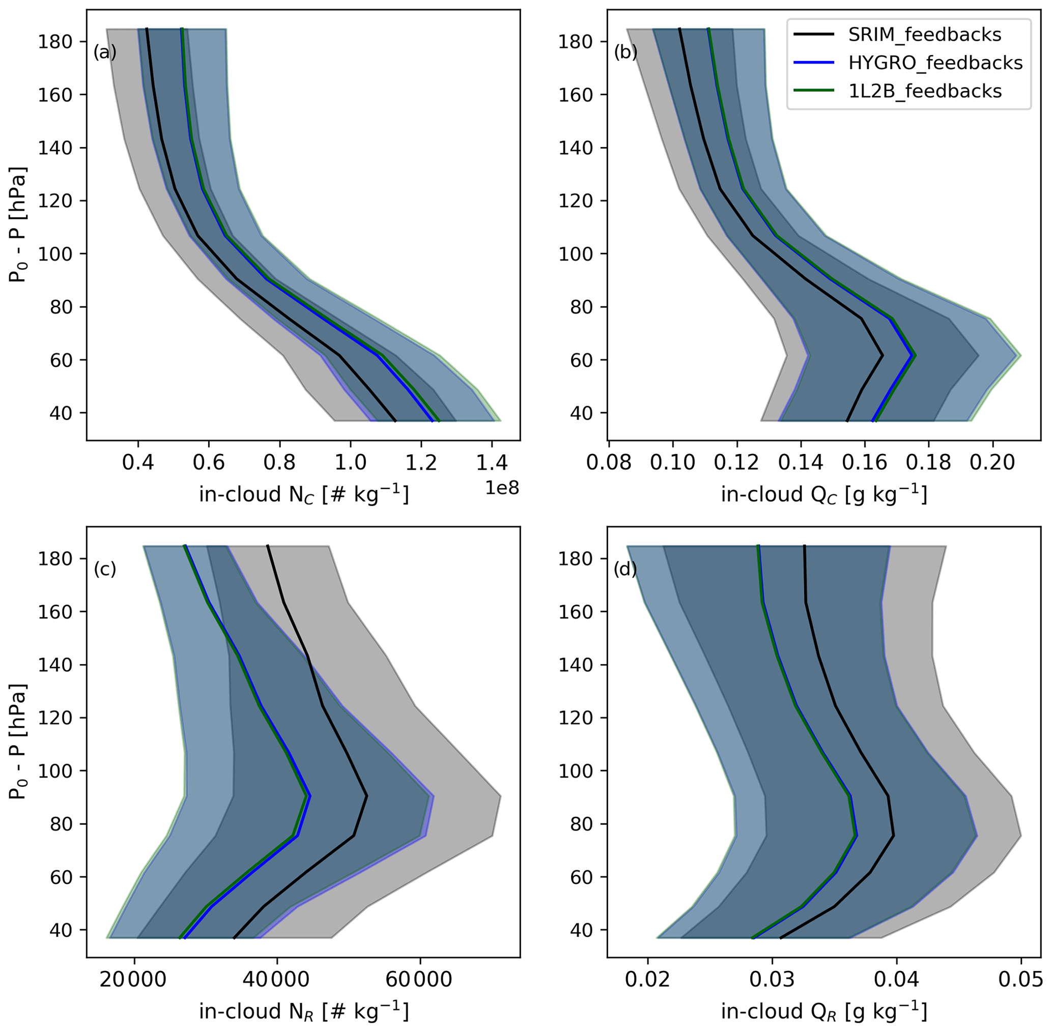
Figure 8Vertical distribution of temporally and horizontally averaged cloud droplet number mixing ratios (NC, a), cloud water mixing ratios (QC, b), raindrop number mixing ratios (NR, c), and rainwater mixing ratios (QR, d) in the SRIM_feedback, HYGRO_feedback, and 1L2B_feedback simulations. The shading indicates 1 temporal standard deviation about the mean.
3.2.1 Aerosol–cloud interactions
In order to target low clouds most likely to be affected by aerosol emitted from the surface, we restrict our analysis to the clouds with model hybrid levels between 0.807 and 0.962, approximately 35–185 hPa below surface pressure. As all cloud variables were saved as 3-hourly means, which will include transitions between cloudy and cloud-free periods, our reported cloud properties will have smaller values than if we had analyzed instantaneous model output. This includes, most notably, the cloud droplet and raindrop number mixing ratios. However, as our interest is in the comparison between simulations, which are all treated identically, this would not alter our conclusions. Additionally, in order to provide more physically meaningful values, when calculating temporally and horizontally averaged cloud properties we define “cloudy” grid cells as those with 3-hourly cloud water mixing ratios (QC) > 0.005 g kg−1, and we filter out grid cells with lower 3-hourly QC values. The mean number of cloudy grid cells differs by less than 0.7 % between simulations (not shown), with the HYGRO_feedback and 1L2B_feedback simulations having slightly more cloudy grid cells than the SRIM_feedback simulation. Therefore differences between simulations are better explained as changes in in-cloud properties, rather than as changes in the spatial extent of clouds. We note that the cloud fraction over the western United States was low during July of 2016, as evidenced in the MODIS satellite retrievals (NASA Earth Observations, https://neo.gsfc.nasa.gov/view.php?datasetId=MODAL2_M_CLD_FR&date=2016-07-28, last access: 19 November 2021).
We show in Fig. 8 the vertical distributions of the temporally and horizontally averaged in-cloud cloud droplet number mixing ratios (NC), cloud water mixing ratios (QC), raindrop number mixing ratios (NR), and rainwater mixing ratios (QR) in the SRIM_feedback, HYGRO_feedback, and 1L2B_feedback simulations. The HYGRO_feedback and 1L2B_feedback model simulations predict NC values that are approximately 15 % larger than in the SRIM_feedback simulation. The difference in NC is approximately constant with altitude. This difference is due to increased aerosol number concentrations, in turn due to both greater aerosol mass concentrations and smaller aerosol diameter, as shown in Fig. 9. These increased NC values lead to mean QC values that are about 7 % greater than in the SRIM_feedback simulation. As NC increases more than QC, the mean cloud droplet size will be decreased in the HYGRO_feedback and 1L2B_feedback simulations. These reduced cloud droplet sizes would be expected to result in reduced autoconversion and slower drizzle formation. Indeed, both NR and QR are reduced in the HYGRO_feedback and 1L2B_feedback simulations relative to the SRIM_feedback simulation, by about 20 % for NR and 9 % for QR. The difference in NC is approximately constant with altitude, while the differences in QC, NR, and QR increase with altitude. For all cloud variables, the differences are slightly larger in the 1L2B_feedback simulation compared to the HYGRO_feedback simulation.
The decreases in in-cloud QR discussed above would be expected to result in decreases in precipitation at the surface. We show the mean precipitation from the SRIM simulation and the effects on precipitation of the HYGRO and 1L2B mixing-state representations in Fig. 10. Many of the differences shown in Fig. 10 include large decreases near large increases. These are due in part to small changes in advection patterns, which subsequently alter the locations of precipitation. We can determine the net effect of the difference in mixing-state representation on surface precipitation by averaging across the domain. When spatially and temporally averaged, the effect of mixing-state representation on precipitation is modest: in the HYGRO_feedback and 1L2B_feedback simulations, the precipitation is reduced by 0.6 % relative to the SRIM_feedback simulation, much smaller than the differences in in-cloud QR discussed above. As the decreases in NR are greater than those in QR, the HYGRO_feedback and 1L2B_feedback simulations would have larger raindrops than the SRIM_feedback simulation, and these larger raindrops would settle to the surface more efficiently, thereby partially offsetting the reduction in QR.
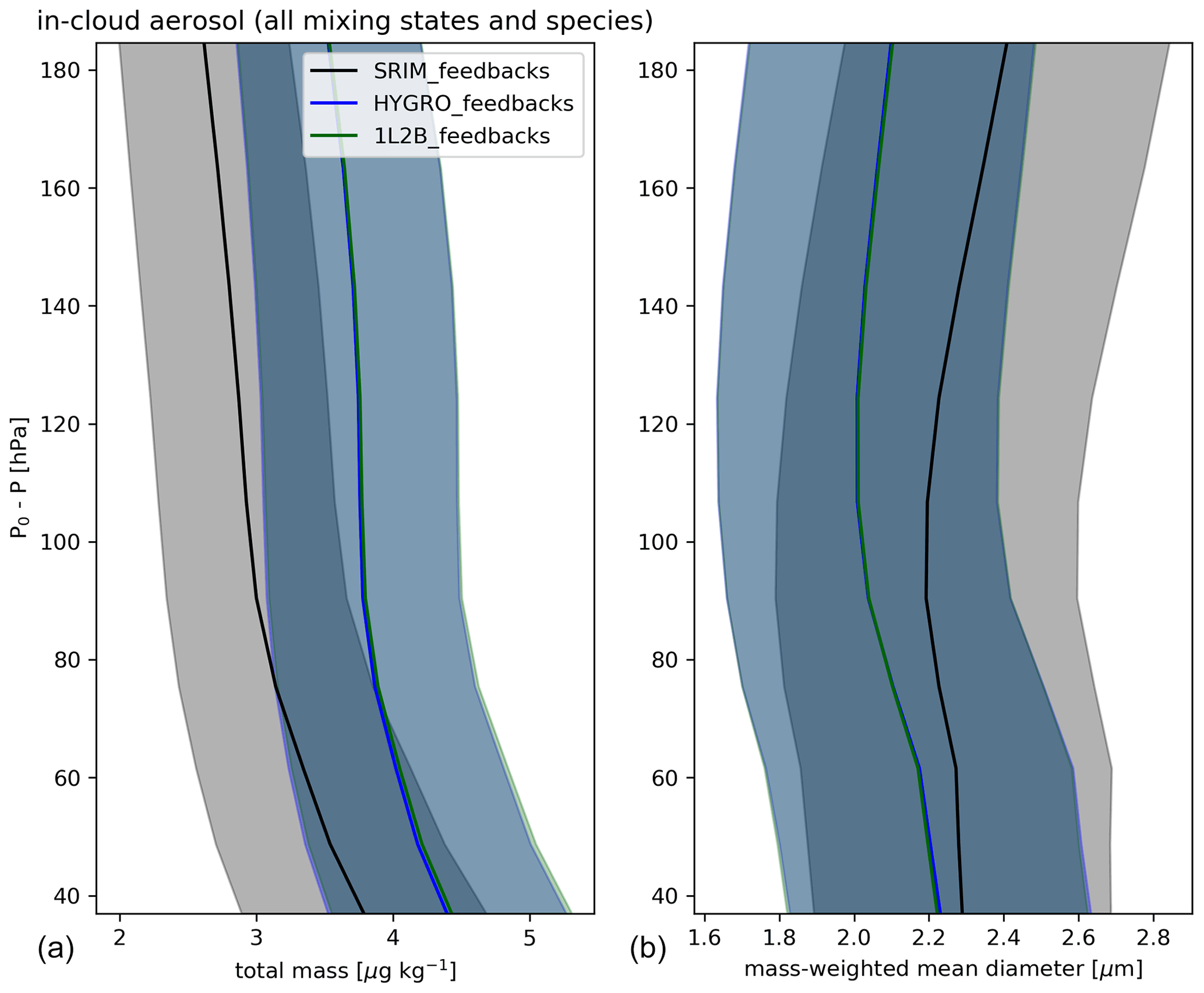
Figure 9Vertical distribution of temporally and horizontally averaged aerosol properties in cloudy grid cells in the SRIM_feedback, HYGRO_feedback, and 1L2B_feedback simulations. (a) Total mass mixing ratios. (b) Mass-mean aerosol diameter. The shading indicates 1 temporal standard deviation about the mean.
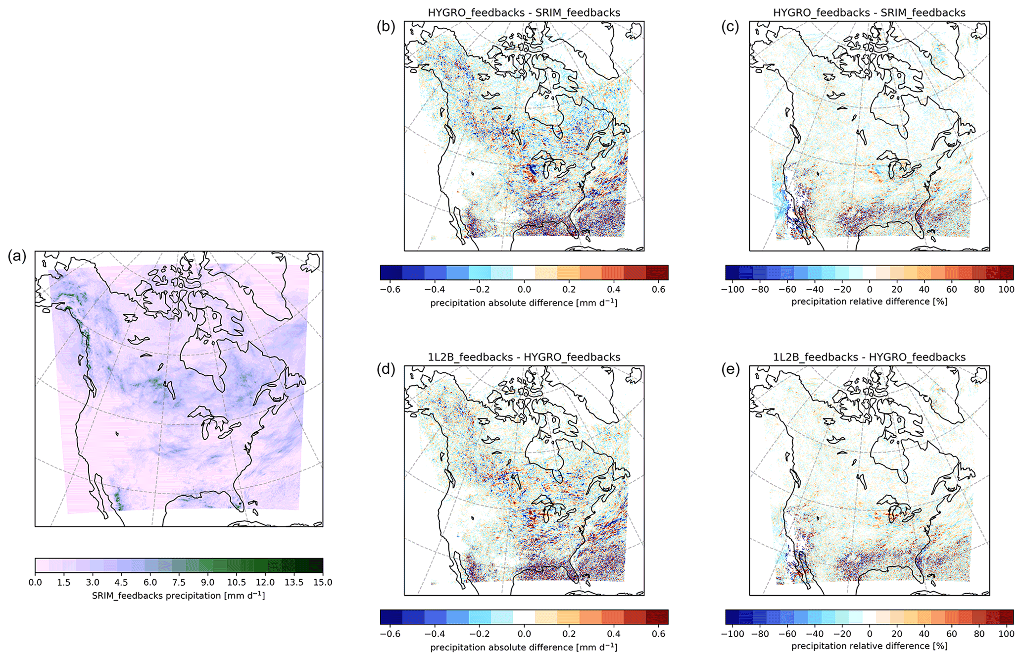
Figure 10(a) Mean precipitation from the SRIM_feedback simulation, (b) mean difference in precipitation between the HYGRO_feedback and SRIM_feedback simulations, (c) relative difference in mean precipitation between the HYGRO_feedback and SRIM_feedback simulations, (d) mean difference in precipitation between the 1L2B_feedback and HYGRO_feedback simulations, and (e) relative difference in mean precipitation between the 1L2B_feedback and HYGRO_feedback simulations.
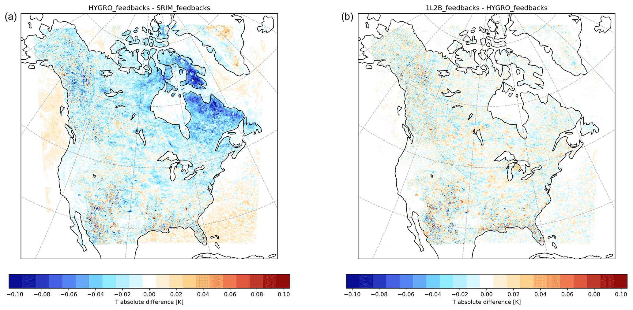
Figure 11(a) Mean difference in surface temperature between the HYGRO_feedback and SRIM_feedback simulations and (b) mean difference in surface temperature between the 1L2B_feedback and HYGRO_feedback simulations.
The increases in NC and QC shown above, along with the small increases in AOD shown in Sect. 3.1.5, would be expected to reduce the shortwave radiation reaching the surface and to potentially reduce surface temperatures. We show in Fig. 11 the differences in mean surface temperatures between the HYGRO_feedback and SRIM_feedback simulations and between the 1L2B_feedback and HYGRO_feedback simulations. Between HYGRO_feedbacks and SRIM_feedbacks, eastern and southern North America show either small differences or noisy differences that would be consistent with slight changes in the locations of clouds. However, there is a clear increase of about 0.01 K over large areas of the oceans and a clear decrease of about 0.06 K over northern Quebec and eastern Nunavut. We note that this region encompasses the outflow of forest fires that occurred in northeastern Canada during the simulation, as is visible in the differences in surface BC mixing ratios (Fig. 4). In the HYGRO_feedback simulation, the emissions from these forest fires are removed more slowly by wet deposition. Therefore, more aerosol particles remain to act as CCN further downwind from the source. The greater CCN concentration increases both NC and QC within the cloud, reducing the solar radiation reaching the surface and reducing surface temperatures. The differences in surface temperatures between 1L2B_feedbacks and HYGRO_feedbacks are noisy throughout the domain, consistent with slight changes in the locations of clouds. We therefore cannot determine any clear effect on surface temperatures due to differences in mixing-state representation between these two simulations.
We note that for all cloud properties, there are only small differences between 1L2B_feedbacks and HYGRO_feedbacks. We remind the reader that the differences in mixing-state representation between 1L2B and HYGRO were designed to capture the effects of correctly resolving the thickness of non-absorbing shells on BC and the subsequent enhancement in aerosol absorption. The effects of these differences in absorption enhancement would be permitted to affect atmospheric temperatures in our simulations, with potential subsequent effects on atmospheric stability. However, we do not find a strong effect on cloud properties, surface precipitation, or surface temperatures in this study. This may be, in part, due to our choice of case study.
In this study, we have implemented a detailed representation of aerosol mixing state into the GEM-MACH air quality and weather forecast model. Our mixing-state representation includes three categories: one for more hygroscopic aerosol, one for less hygroscopic aerosol with a high BC mass fraction, and one for less hygroscopic aerosol with a low BC mass fraction. Currently, the HYGRO and 1L2B configurations require approximately 70 % and 150 % more running-time, respectively, than the SRIM configuration. We expect to reduce this additional cost through improvements to the efficiency of the model tracer transport scheme in the near future. The more detailed representation allowed us to better resolve two different aspects of aerosol mixing state: first, differences in hygroscopicity due to differences in aerosol composition, including the change in hygroscopicity with time as less hygroscopic aerosol becomes coated with hydrophilic material, and, second, the thickness of non-absorbing coatings on BC aerosol which enhance the absorption of the BC aerosol.
We compared the results of the three-category representation (1L2B) with a simulation that uses two categories, split by hygroscopicity (HYGRO), and a simulation using the original size-resolved internally mixed assumption (SRIM). We showed that when we included one or two categories of less hygroscopic aerosol, wet deposition of BC, POA, SOA, and dust was reduced, yielding increases in the mean concentrations of these species of 16 %–93 % and an increase in the mean PM2.5 concentration by 23 %. The effect on dust concentrations is likely overestimated, as the current implementation prevents in-cloud scavenging of aerosol in the hydrophobic category, even if the aerosol is large. We intend to improve on this in a future version of GEM-MACH. As BC, POA, and SOA mass is more concentrated in smaller aerosol particles, we believe that the reduction of wet deposition in these species is realistic. The increased PM2.5 concentrations led to an increase in the AQHI2.5 by 0.05 units on average. The increases in aerosol concentrations also led to increases in both AOD and AAOD.
We briefly compared the results of the SRIM and 1L2B simulations and observations from the IMPROVE, CSN and AQS networks. However, we did not find significant improvement in model–observation agreement with the more detailed mixing-state representation. The reduced wet deposition worsened an existing high bias in BC, organic matter, and dust concentrations, and we saw only small changes in correlation with the observations. It is likely that a more thorough assessment will require observations from sites that are strongly affected by long-range transport of BC and organic aerosol. The CSN network sites in particular are located in urban centres and would therefore be expected to be weakly affected by changes in wet deposition. We will investigate this further in future work.
However, using two categories to resolve more hygroscopic and less hygroscopic aerosol only yielded modest improvements in resolving the amount of coating material on BC particles, which alters their absorption of solar radiation. We found that using three mixing-state categories (more hygroscopic aerosol, less hygroscopic high BC mass fraction aerosol, and less hygroscopic low BC mass fraction aerosol) allowed us to distinguish thinly coated BC from BC that was thickly coated with POA. This yielded a mean AAOD that was 3 % less than when separating the aerosol by hygroscopicity alone. Many sources of BC are also sources of POA, and observations indicate that the BC-containing particles frequently also contain POA, even close to emission sources (Perring et al., 2017; Kondo et al., 2011). We note that we assumed that particles from area sources were externally mixed at emission. This assumption will yield a maximum difference between our sensitivity simulations. Nonetheless, as thinly coated BC particles have been observed in the ambient atmosphere, even far from emission sources (Zanatta et al., 2018; Sharma et al., 2017), it is clear that POA and BC are not evenly distributed across particles in the same size range. The proportion of POA that is emitted as BC-containing particles vs. BC-free particles is currently poorly constrained. We therefore suggest that future observation campaigns record not only the coating thickness on BC-containing particles, but also, when possible, the proportion of organic matter that exists as BC-free particles vs. BC-containing particles.
We then performed simulations that included aerosol feedbacks on meteorology in order to determine the effects of mixing-state representation on the forecast meteorology. We found a clear effect due to including two categories of aerosol hygroscopicity: the increased aerosol concentrations due to the decreases in wet deposition increased cloud droplet mixing ratios by approximately 15 %. This led to a reduction in the mean precipitation by 0.6 %. The increased cloud reflectivity resulted in a decrease in surface temperatures by about 0.06 K over northeastern Canada, in the outflow of large forest fires. When we compared the results of the HYGRO simulation with those of the 1L2B simulation, which better resolves BC mass fraction and aerosol absorption, we did not find a strong effect on forecast meteorology.
GEM-MACH, the atmospheric chemistry library for the GEM numerical atmospheric model (© 2007–2013, Air Quality Research Division and National Prediction Operations Division, Environment and Climate Change Canada), is free software which can be redistributed and/or modified under the terms of the GNU Lesser General Public License as published by the Free Software Foundation – either version 2.1 of the license or any later version. The GEM (meteorology) code (CMC, 2021) is available to download from https://github.com/mfvalin?tab=repositories (last access: 27 April 2022). The specific GM-MixingState version used in this work may be obtained on request to Ashu Dastoor (ashu.dastoor@canada.ca). The executable for GEM-MACH is obtained by providing the chemistry library to GEM when generating its executable.
The observed data sets we used for comparison were downloaded from IMPROVE (http://vista.cira.colostate.edu/Improve/, last access: 3 March 2022, IMPROVE Network, 2022), and the US EPA AQS (https://www.epa.gov/aqs, last access: 3 March 2022, US EPA, 2022), as mentioned in the text. The model output is available upon request to Ashu Dastoor (ashu.dastoor@ec.gc.ca).
The supplement related to this article is available online at: https://doi.org/10.5194/acp-22-13527-2022-supplement.
RS designed and implemented the novel mixing-state representations in GEM-MACH. RS led the writing and preparation of the manuscript. RS and AR performed the computational experiments and led the analysis. MM designed and implemented improved aerosol–radiation interactions in GEM-MACH. AD provided project oversight and guidance.
The contact author has declared that none of the authors has any competing interests.
Publisher’s note: Copernicus Publications remains neutral with regard to jurisdictional claims in published maps and institutional affiliations.
We would like to thank Ayodeji Akingunola, Alexandru Lupu, and Craig Stroud of Air Quality Research Division of Environment and Climate Change Canada for their expertise and contributions in this project.
This paper was edited by Joshua Fu and reviewed by four anonymous referees.
Abdul-Razzak, H. and Ghan, S. J.: A parameterization of aerosol activation 3, Sectional representation, J. Geophys. Res., 107, 4026, https://doi.org/10.1029/2001JD000483, 2002. a, b, c
Adachi, K., Chung, S. H., and Buseck, P. R.: Shapes of soot aerosol particles and implications for their effects on climate, J. Geophys. Res., 115, D15206, https://doi.org/10.1029/2009JD012868, 2010. a
Akingunola, A., Makar, P. A., Zhang, J., Darlington, A., Li, S. M., Gordon, M., Moran, M. D., and Zheng, Q.: A chemical transport model study of plume-rise and particle size distribution for the Athabasca oil sands, Atmos. Chem. Phys., 18, 8667–8688, https://doi.org/10.5194/acp-18-8667-2018, 2018. a
Andersson, C., Bergström, R., Bennet, C., Robertson, L., Thomas, M., Korhonen, H., Lehtinen, K. E. J., and Kokkola, H.: MATCH-SALSA – Multi-scale Atmospheric Transport and CHemistry model coupled to the SALSA aerosol microphysics model – Part 1: Model description and evaluation, Geosci. Model Dev., 8, 171–189, https://doi.org/10.5194/gmd-8-171-2015, 2015. a, b
Anttila, T.: Sensitivity of cloud droplet formation to the numerical treatment of the particle mixing state, J. Geophys. Res., 115, D21205, https://doi.org/10.1029/2010jd013995, 2010. a
Appel, K. W., Pouliot, G. A., Simon, H., Sarwar, G., Pye, H. O. T., Napelenok, S. L., Akhtar, F., and Roselle, S. J.: Evaluation of dust and trace metal estimates from the Community Multiscale Air Quality (CMAQ) model version 5.0, Geosci. Model Dev., 6, 883–899, https://doi.org/10.5194/gmd-6-883-2013, 2013. a, b
Aquila, V., Hendricks, J., Lauer, A., Riemer, N., Vogel, H., Baumgardner, D., Minikin, A., Petzold, A., Schwarz, J. P., Spackman, J. R., Weinzierl, B., Righi, M., and Dall'Amico, M.: MADE-in: a new aerosol microphysics submodel for global simulation of insoluble particles and their mixing state, Geosci. Model Dev., 4, 325–355, https://doi.org/10.5194/gmd-4-325-2011, 2011. a, b
Bellouin, N., Mann, G. W., Woodhouse, M. T., Johnson, C., Carslaw, K. S., and Dalvi, M.: Impact of the modal aerosol scheme GLOMAP-mode on aerosol forcing in the Hadley Centre Global Environmental Model, Atmos. Chem. Phys., 13, 3027–3044, https://doi.org/10.5194/acp-13-3027-2013, 2013. a, b
Bergman, T., Kerminen, V.-M., Korhonen, H., Lehtinen, K. J., Makkonen, R., Arola, A., Mielonen, T., Romakkaniemi, S., Kulmala, M., and Kokkola, H.: Evaluation of the sectional aerosol microphysics module SALSA implementation in ECHAM5-HAM aerosol-climate model, Geosci. Model Dev., 5, 845–868, https://doi.org/10.5194/gmd-5-845-2012, 2012. a, b
Bey, I., Jacob, D. J., Yantosca, R. M., Logan, J. A., Field, B. D., Fiore, A. M., Li, Q., Liu, H. Y., Mickley, L. J., and Schultz, M. G.: Global modeling of tropospheric chemistry with assimilated meteorology: Model description and evaluation, J. Geophys. Res.-Atmos., 106, 23073–23095, https://doi.org/10.1029/2001JD000807, 2001. a, b
Bieser, J., Aulinger, A., Matthias, V., Quante, M., and Builtjes, P.: SMOKE for Europe – adaptation, modification and evaluation of a comprehensive emission model for Europe, Geosci. Model Dev., 4, 47–68, https://doi.org/10.5194/gmd-4-47-2011, 2011. a
Binkowski, F. S. and Roselle, S. J.: Models-3 Community Multiscale Air Quality (CMAQ) model aerosol component 1. Model description, J. Geophys. Res., 108, 4183, https://doi.org/10.1029/2001JD001409, 2003. a, b
Bond, T. C., Habib, G., and Bergstrom, R. W.: Limitations in the enhancement of visible light absorption due to mixing state, J. Geophys. Res., 111, D20211, https://doi.org/10.1029/2006JD007315, 2006. a, b
Bond, T. C., Doherty, S. J., Fahey, D. W., Forster, P. M., Berntsen, T., DeAngelo, B. J., Flanner, M. G., Ghan, S., Kärcher, B., Koch, D., Kinne, S., Kondo, Y., Quinn, P. K., Sarofim, M. C., Schultz, M. G., Schulz, M., Venkataraman, C., Zhang, H., Zhang, S., Bellouin, N., Guttikunda, S. K., Hopke, P. K., Jacobson, M. Z., Kaiser, J. W., Klimont, Z., Lohmann, U., Schwarz, J. P., Shindell, D., Storelvmo, T., Warren, S. G., and Zender, C. S.: Bounding the role of black carbon in the climate system: A scientific assessment, J. Geophys. Res.-Atmos., 118, 5380–5552, https://doi.org/10.1002/jgrd.50171, 2013. a
Boucher, O., Randall, D., Artaxo, P., Bretherton, C., Feingold, G., Forster, P., Kerminen, V.-M. M., Kondo, Y., Liao, H., Lohmann, U., Rasch, P., Satheesh, S. K., Sherwood, S., Stevens, B., and Zhang, X. Y.: Clouds and Aerosols, in: Climate Change 2013: The Physical Science Basis. Contribution of Working Group I to the Fifth Assessment Report of the Intergovernmental Panel on Climate Change, edited by: Stocker, T., Qin, D., Plattner, G.-K., Tignor, M., Allen, S., Boschung, J., Nauels, A., Xia, Y., Bex, V., and Midgley, P., 571–657, Cambridge University Press, Cambridge, United Kingdom and New York, NY, USA, ISBN 9781107415324, https://doi.org/10.1017/CBO9781107415324, 2013. a
Cappa, C. D., Onasch, T. B., Massoli, P., Worsnop, D. R., Bates, T. S., Cross, E. S., Davidovits, P., Hakala, J., Hayden, K. L., Jobson, B. T., Kolesar, K. R., Lack, D. A., Lerner, B. M., Li, S. M., Mellon, D., Nuaaman, I., Olfert, J. S., Petaja, T., Quinn, P. K., Song, C., Subramanian, R., Williams, E. J., and Zaveri, R. A.: Radiative Absorption Enhancements Due to the Mixing State of Atmospheric Black Carbon, Science, 337, 1078–1081, https://doi.org/10.1126/science.1223447, 2012. a
Charron, M., Polavarapu, S., Buehner, M., Vaillancourt, P. A., Charette, C., Roch, M., Morneau, J., Garand, L., Aparicio, J. M., MacPherson, S., Pellerin, S., St-James, J., and Heilliette, S.: The Stratospheric Extension of the Canadian Global Deterministic Medium-Range Weather Forecasting System and Its Impact on Tropospheric Forecasts, Mon. Weather Rev., 140, 1924–1944, https://doi.org/10.1175/MWR-D-11-00097.1, 2012. a
Chen, J., Anderson, K., Pavlovic, R., Moran, M. D., Englefield, P., Thompson, D. K., Munoz-Alpizar, R., and Landry, H.: The FireWork v2.0 air quality forecast system with biomass burning emissions from the Canadian Forest Fire Emissions Prediction System v2.03, Geosci. Model Dev., 12, 3283–3310, https://doi.org/10.5194/gmd-12-3283-2019, 2019. a
Ching, J., Zaveri, R. A., Easter, R. C., Riemer, N., and Fast, J. D.: A three-dimensional sectional representation of aerosol mixing state for simulating optical properties and cloud condensation nuclei, J. Geophys. Res.-Atmos., 121, 5912–5929, https://doi.org/10.1002/2015jd024323, 2016. a, b, c
Cohard, J.-M. and Pinty, J.-P.: A comprehensive two-moment warm microphysical bulk scheme. I: Description and tests, Q. J. Roy. Meteorol. Soc., 126, 1815–1842, https://doi.org/10.1002/qj.49712656613, 2010. a
Côté, J., Desmarais, J.-G., Gravel, S., Méthot, A., Patoine, A., Roch, M., and Staniforth, A.: The Operational CMC–MRB Global Environmental Multiscale (GEM) Model, Part II: Results, Mon. Weather Rev., 126, 1397–1418, https://doi.org/10.1175/1520-0493(1998)126<1397:TOCMGE>2.0.CO;2, 1998a. a
Côté, J., Gravel, S., Méthot, A., Patoine, A., Roch, M., and Staniforth, A.: The Operational CMC-MRB Global Environmental Multiscale (GEM) Model. Part I: Design Considerations and Formulation, Mon. Weather Rev., 126, 1373–1395, https://doi.org/10.1175/1520-0493(1998)126<1373:TOCMGE>2.0.CO;2, 1998b. a
Cui, X., Wang, X., Yang, L., Chen, B., Chen, J., Andersson, A., and Gustafsson, O.: Radiative absorption enhancement from coatings on black carbon aerosols, Sci. Total Environ., 551/552, 51–56, https://doi.org/10.1016/j.scitotenv.2016.02.026, 2016. a
Dalirian, M., Ylisirniö, A., Buchholz, A., Schlesinger, D., Ström, J., Virtanen, A., and Riipinen, I.: Cloud droplet activation of black carbon particles coated with organic compounds of varying solubility, Atmos. Chem. Phys., 18, 12477–12489, https://doi.org/10.5194/acp-18-12477-2018, 2018. a
Elleman, R. A. and Covert, D. S.: Aerosol size distribution modeling with the Community Multiscale Air Quality modeling system in the Pacific Northwest: 1. Model comparison to observations, J. Geophys. Res., 114, D11206, https://doi.org/10.1029/2008JD010791, 2009. a, b
Emmons, L. K., Walters, S., Hess, P. G., Lamarque, J.-F., Pfister, G. G., Fillmore, D., Granier, C., Guenther, A., Kinnison, D., Laepple, T., Orlando, J., Tie, X., Tyndall, G., Wiedinmyer, C., Baughcum, S. L., and Kloster, S.: Description and evaluation of the Model for Ozone and Related chemical Tracers, version 4 (MOZART-4), Geosci. Model Dev., 3, 43–67, https://doi.org/10.5194/gmd-3-43-2010, 2010. a, b, c
Fung, C., Misra, P., Bloxam, R., and Wong, S.: A numerical experiment on the relative importance of H2O2 O3 in aqueous conversion of SO2 to SO, Atmos. Environ. Pt. A, 25, 411–423, https://doi.org/10.1016/0960-1686(91)90312-U, 1991. a
Galmarini, S., Makar, P., Clifton, O. E., Hogrefe, C., Bash, J. O., Bellasio, R., Bianconi, R., Bieser, J., Butler, T., Ducker, J., Flemming, J., Hodzic, A., Holmes, C. D., Kioutsioukis, I., Kranenburg, R., Lupascu, A., Perez-Camanyo, J. L., Pleim, J., Ryu, Y.-H., San Jose, R., Schwede, D., Silva, S., and Wolke, R.: Technical note: AQMEII4 Activity 1: evaluation of wet and dry deposition schemes as an integral part of regional-scale air quality models, Atmos. Chem. Phys., 21, 15663–15697, https://doi.org/10.5194/acp-21-15663-2021, 2021. a, b
Gong, S. L.: A parameterization of sea-salt aerosol source function for sub- and super-micron particles, Global Biogeochem. Cy., 17, 1097, https://doi.org/10.1029/2003gb002079, 2003. a
Gong, S. L., Barrie, L. A., and Lazare, M.: Canadian Aerosol Module: A size-segregated simulation of atmospheric aerosol processes for climate and air quality models 1. Module development, J. Geophys. Res., 108, 4007, https://doi.org/10.1029/2001JD002002, 2003. a, b
Gong, W., Dastoor, A. P., Bouchet, V. S., Gong, S., Makar, P. A., Moran, M. D., Pabla, B., Ménard, S., Crevier, L.-P., Cousineau, S., and Venkatesh, S.: Cloud processing of gases and aerosols in a regional air quality model (AURAMS), Atmos. Res., 82, 248–275, https://doi.org/10.1016/j.atmosres.2005.10.012, 2006. a, b, c
Gong, W., Makar, P., Zhang, J., Milbrandt, J., Gravel, S., Hayden, K., Macdonald, A., and Leaitch, W.: Modelling aerosol–cloud–meteorology interaction: A case study with a fully coupled air quality model (GEM-MACH), Atmos. Environ., 115, 695–715, https://doi.org/10.1016/j.atmosenv.2015.05.062, 2015. a, b, c, d
Han, X., Zhang, M., Zhu, L., and Xu, L.: Model analysis of influences of aerosol mixing state upon its optical properties in East Asia, Adv. Atmos. Sci., 30, 1201–1212, https://doi.org/10.1007/s00376-012-2150-4, 2013. a
Hogrefe, C., Sistla, G., Zalewsky, E., Hao, W., and Ku, J.-Y.: An Assessment of the Emissions Inventory Processing Systems EMS-2001 and SMOKE in Grid-Based Air Quality Models, J. Air Waste Manag. Assoc., 53, 1121–1129, https://doi.org/10.1080/10473289.2003.10466261, 2003. a
Houyoux, M. R., Vukovich, J. M., Coats, C. J., Wheeler, N. J. M., and Kasibhatla, P. S.: Emission inventory development and processing for the Seasonal Model for Regional Air Quality (SMRAQ) project, J. Geophys. Res.-Atmos., 105, 9079–9090, https://doi.org/10.1029/1999JD900975, 2000. a
IMPROVE Network: Federal Land Manager Environmental Database [data set], http://vista.cira.colostate.edu/Improve/, last access: 3 March 2022. a
Kaiser, J. C., Hendricks, J., Righi, M., Riemer, N., Zaveri, R. A., Metzger, S., and Aquila, V.: The MESSy aerosol submodel MADE3 (v2.0b): Description and a box model test, Geosci. Model Dev., 7, 1137–1157, https://doi.org/10.5194/gmd-7-1137-2014, 2014. a, b
Kaiser, J. C., Hendricks, J., Righi, M., Jöckel, P., Tost, H., Kandler, K., Weinzierl, B., Sauer, D., Heimerl, K., Schwarz, J. P., Perring, A. E., and Popp, T.: Global aerosol modeling with MADE3 (v3.0) in EMAC (based on v2.53): model description and evaluation, Geosci. Model Dev., 12, 541–579, https://doi.org/10.5194/gmd-12-541-2019, 2019. a, b
Khalizov, A. F., Xue, H., Wang, L., Zheng, J., and Zhang, R.: Enhanced Light Absorption and Scattering by Carbon Soot Aerosol Internally Mixed with Sulfuric Acid, J. Phys. Chem. A, 113, 1066–1074, https://doi.org/10.1021/jp807531n, 2009. a
Kim, N., Park, M., Yum, S. S., Park, J. S., Shin, H. J., and Ahn, J. Y.: Impact of urban aerosol properties on cloud condensation nuclei (CCN) activity during the KORUS-AQ field campaign, Atmos. Environ., 185, 221–236, https://doi.org/10.1016/j.atmosenv.2018.05.019, 2018. a
Klingmüller, K., Steil, B., Brühl, C., Tost, H., and Lelieveld, J.: Sensitivity of aerosol radiative effects to different mixing assumptions in the AEROPT 1.0 submodel of the EMAC atmospheric-chemistry–climate model, Geosci. Model Dev., 7, 2503–2516, https://doi.org/10.5194/gmd-7-2503-2014, 2014. a, b
Koehler, K. A., Kreidenweis, S. M., DeMott, P. J., Petters, M. D., Prenni, A. J., and Carrico, C. M.: Hygroscopicity and cloud droplet activation of mineral dust aerosol, Geophys. Res. Lett., 36, L08805, https://doi.org/10.1029/2009GL037348, 2009. a
Kokkola, H., Korhonen, H., Lehtinen, K. E. J., Makkonen, R., Asmi, A., Järvenoja, S., Anttila, T., Partanen, A.-I., Kulmala, M., Järvinen, H., Laaksonen, A., and Kerminen, V.-M.: SALSA – a sectional aerosol module for large scale applications, Atmos. Chem. Phys., 8, 2469–2483, https://doi.org/10.5194/acp-8-2469-2008, 2008. a, b
Kokkola, H., Kühn, T., Laakso, A., Bergman, T., Lehtinen, K. E. J., Mielonen, T., Arola, A., Stadtler, S., Korhonen, H., Ferrachat, S., Lohmann, U., Neubauer, D., Tegen, I., Siegenthaler-Le Drian, C., Schultz, M. G., Bey, I., Stier, P., Daskalakis, N., Heald, C. L., and Romakkaniemi, S.: SALSA2.0: The sectional aerosol module of the aerosol–chemistry–climate model ECHAM6.3.0-HAM2.3-MOZ1.0, Geosci. Model Dev., 11, 3833–3863, https://doi.org/10.5194/gmd-11-3833-2018, 2018. a, b
Kondo, Y., Matsui, H., Moteki, N., Sahu, L., Takegawa, N., Kajino, M., Zhao, Y., Cubison, M. J., Jimenez, J. L., Vay, S., Diskin, G. S., Anderson, B., Wisthaler, A., Mikoviny, T., Fuelberg, H. E., Blake, D. R., Huey, G., Weinheimer, A. J., Knapp, D. J., and Brune, W. H.: Emissions of black carbon, organic, and inorganic aerosols from biomass burning in North America and Asia in 2008, J. Geophys. Res., 116, D08204, https://doi.org/10.1029/2010JD015152, 2011. a, b, c
Lack, D. A., Langridge, J. M., Bahreini, R., Cappa, C. D., Middlebrook, A. M., and Schwarz, J. P.: Brown carbon and internal mixing in biomass burning particles, P. Natl. Acad. Sci. USA, 109, 14802–14807, https://doi.org/10.1073/pnas.1206575109, 2012. a
Lauer, A., Hendricks, J., Ackermann, I., Schell, B., Hass, H., and Metzger, S.: Simulating aerosol microphysics with the ECHAM/MADE GCM – Part I: Model description and comparison with observations, Atmos. Chem. Phys., 5, 3251–3276, https://doi.org/10.5194/acp-5-3251-2005, 2005. a, b
Lee, L. a., Pringle, K. J., Reddington, C. L., Mann, G. W., Stier, P., Spracklen, D. V., Pierce, J. R., and Carslaw, K. S.: The magnitude and causes of uncertainty in global model simulations of cloud condensation nuclei, Atmos. Chem. Phys., 13, 8879–8914, https://doi.org/10.5194/acp-13-8879-2013, 2013. a
Lesins, G., Chylek, P., and Lohmann, U.: A study of internal and external mixing scenarios and its effect on aerosol optical properties and direct radiative forcing, J. Geophys. Res.-Atmos., 107, 4094, https://doi.org/10.1029/2001jd000973, 2002. a
Liu, D., Whitehead, J., Alfarra, M. R., Reyes-Villegas, E., Spracklen, D. V., Reddington, C. L., Kong, S., Williams, P. I., Ting, Y.-C., Haslett, S., Taylor, J. W., Flynn, M. J., Morgan, W. T., McFiggans, G., Coe, H., and Allan, J. D.: Black-carbon absorption enhancement in the atmosphere determined by particle mixing state, Nat. Geosci., 10, 184–188, https://doi.org/10.1038/ngeo2901, 2017. a
Liu, L. and Mishchenko, M.: Scattering and Radiative Properties of Morphologically Complex Carbonaceous Aerosols: A Systematic Modeling Study, Remote Sens., 10, 1634, https://doi.org/10.3390/rs10101634, 2018. a
Liu, S., Aiken, A. C., Gorkowski, K., Dubey, M. K., Cappa, C. D., Williams, L. R., Herndon, S. C., Massoli, P., Fortner, E. C., Chhabra, P. S., Brooks, W. A., Onasch, T. B., Jayne, J. T., Worsnop, D. R., China, S., Sharma, N., Mazzoleni, C., Xu, L., Ng, N. L., Liu, D., Allan, J. D., Lee, J. D., Fleming, Z. L., Mohr, C., Zotter, P., Szidat, S., and Prévôt, A. S. H.: Enhanced light absorption by mixed source black and brown carbon particles in UK winter, Nat. Commun., 6, 8435, https://doi.org/10.1038/ncomms9435, 2015. a
Liu, X., Easter, R. C., Ghan, S. J., Zaveri, R., Rasch, P., Shi, X., Lamarque, J. F., Gettelman, A., Morrison, H., Vitt, F., Conley, A., Park, S., Neale, R., Hannay, C., Ekman, A. M. L., Hess, P., Mahowald, N., Collins, W., Iacono, M. J., Bretherton, C. S., Flanner, M. G., and Mitchell, D.: Toward a minimal representation of aerosols in climate models: description and evaluation in the Community Atmosphere Model CAM5, Geosci. Model Dev., 5, 709–739, https://doi.org/10.5194/gmd-5-709-2012, 2012. a, b, c, d, e
Liu, X., Ma, P.-L. L., Wang, H., Tilmes, S., Singh, B., Easter, R. C., Ghan, S. J., and Rasch, P. J.: Description and evaluation of a new four-mode version of the Modal Aerosol Module (MAM4) within version 5.3 of the Community Atmosphere Model, Geosci. Model Dev., 9, 505–522, https://doi.org/10.5194/gmd-9-505-2016, 2016. a, b, c, d
Majdzadeh, M., Stroud, C. A., Sioris, C., Makar, P. A., Akingunola, A., McLinden, C., Zhao, X., Moran, M. D., Abboud, I., and Chen, J.: Development of aerosol optical properties for improving the MESSy photolysis module in the GEM-MACH v2.4 air quality model and application for calculating photolysis rates in a biomass burning plume, Geosci. Model Dev., 15, 219–249, https://doi.org/10.5194/gmd-15-219-2022, 2022. a, b, c
Makar, P., Bouchet, V., and Nenes, A.: Inorganic chemistry calculations using HETV – a vectorized solver for the SO–NO3–NH4+ system based on the ISORROPIA algorithms, Atmos. Environ., 37, 2279–2294, https://doi.org/10.1016/S1352-2310(03)00074-8, 2003. a
Makar, P. A., Gong, W., Hogrefe, C., Zhang, Y., Curci, G., Žabkar, R., Milbrandt, J., Im, U., Balzarini, A., Baró, R., Bianconi, R., Cheung, P., Forkel, R., Gravel, S., Hirtl, M., Honzak, L., Hou, A., Jiménez-Guerrero, P., Langer, M., Moran, M. D., Pabla, B., Pérez, J. L., Pirovano, G., San José, R., Tuccella, P., Werhahn, J., Zhang, J., Galmarini, S., Hogrefe, C., Zhang, Y., Curci, G., Žabkar, R., Im, U., Balzarini, A., Baró, R., Bianconi, R., Cheung, P., Forkel, R., Gravel, S., Hirtl, M., Honzak, L., Hou, A., Jiménez-Guerrero, P., Langer, M., Moran, M. D., Pabla, B., Pérez, J. L., Pirovano, G., San José, R., Tuccella, P., Werhahn, J., Zhang, J., Galmarini, S., Milbrandt, J., Im, U., Balzarini, A., Baró, R., Bianconi, R., Cheung, P., Forkel, R., Gravel, S., Hirtl, M., Honzak, L., Hou, A., Jiménez-Guerrero, P., Langer, M., Moran, M. D., Pabla, B., Pérez, J. L., Pirovano, G., San José, R., Tuccella, P., Werhahn, J., Zhang, J., Galmarini, S., Hogrefe, C., Zhang, Y., Curci, G., Žabkar, R., Im, U., Balzarini, A., Baró, R., Bianconi, R., Cheung, P., Forkel, R., Gravel, S., Hirtl, M., Honzak, L., Hou, A., Jiménez-Guerrero, P., Langer, M., Moran, M. D., Pabla, B., Pérez, J. L., Pirovano, G., San José, R., Tuccella, P., Werhahn, J., Zhang, J., and Galmarini, S.: Feedbacks between air pollution and weather, Part 1: Effects on weather, Atmos. Environ., 115, 442–469, https://doi.org/10.1016/j.atmosenv.2014.12.003, 2015a. a
Makar, P. A., Gong, W., Hogrefe, C., Zhang, Y., Curci, G., Žabkar, R., Milbrandt, J., Im, U., Balzarini, A., Baró, R., Bianconi, R., Cheung, P., Forkel, R., Gravel, S., Hirtl, M., Honzak, L., Hou, A., Jiménez-Guerrero, P., Langer, M., Moran, M. D., Pabla, B., Pérez, J. L., Pirovano, G., San José, R., Tuccella, P., Werhahn, J., Zhang, J., Galmarini, S., Hogrefe, C., Zhang, Y., Curci, G., Žabkar, R., Im, U., Balzarini, A., Baró, R., Bianconi, R., Cheung, P., Forkel, R., Gravel, S., Hirtl, M., Honzak, L., Hou, A., Jiménez-Guerrero, P., Langer, M., Moran, M. D., Pabla, B., Pérez, J. L., Pirovano, G., San José, R., Tuccella, P., Werhahn, J., Zhang, J., Galmarini, S., Milbrandt, J., Im, U., Balzarini, A., Baró, R., Bianconi, R., Cheung, P., Forkel, R., Gravel, S., Hirtl, M., Honzak, L., Hou, A., Jiménez-Guerrero, P., Langer, M., Moran, M. D., Pabla, B., Pérez, J. L., Pirovano, G., San José, R., Tuccella, P., Werhahn, J., Zhang, J., Galmarini, S., Hogrefe, C., Zhang, Y., Curci, G., Žabkar, R., Im, U., Balzarini, A., Baró, R., Bianconi, R., Cheung, P., Forkel, R., Gravel, S., Hirtl, M., Honzak, L., Hou, A., Jiménez-Guerrero, P., Langer, M., Moran, M. D., Pabla, B., Pérez, J. L., Pirovano, G., San José, R., Tuccella, P., Werhahn, J., Zhang, J., and Galmarini, S.: Feedbacks between air pollution and weather, part 2: Effects on chemistry, Atmos. Environ., 115, 442–469, https://doi.org/10.1016/j.atmosenv.2014.10.021, 2015b. a
Manktelow, P. T., Carslaw, K. S., Mann, G. W., and Spracklen, D. V.: The impact of dust on sulfate aerosol, CN and CCN during an East Asian dust storm, Atmos. Chem. Phys., 10, 365–382, https://doi.org/10.5194/acp-10-365-2010, 2010. a, b
Mann, G. W., Carslaw, K. S., Spracklen, D. V., Ridley, D. A., Manktelow, P. T., Chipperfield, M. P., Pickering, S. J., and Johnson, C. E.: Description and evaluation of GLOMAP-mode: a modal global aerosol microphysics model for the UKCA composition-climate model, Geosci. Model Dev., 3, 519–551, https://doi.org/10.5194/gmd-3-519-2010, 2010. a, b
Matsui, H.: Development of a global aerosol model using a two-dimensional sectional method: 1. Model design, J. Adv. Model. Earth Syst., 9, 1921–1947, https://doi.org/10.1002/2017ms000936, 2017. a, b
Matsui, H., Koike, M., Kondo, Y., Moteki, N., Fast, J. D., and Zaveri, R. A.: Development and validation of a black carbon mixing state resolved three-dimensional model: Aging processes and radiative impact, J. Geophys. Res.-Atmos., 118, 2304–2326, https://doi.org/10.1029/2012JD018446, 2013. a
Matsui, H., Koike, M., Kondo, Y., Fast, J. D., and Takigawa, M.: Development of an aerosol microphysical module: Aerosol Two-dimensional bin module for foRmation and Aging Simulation (ATRAS), Atmos. Chem. Phys., 14, 10315–10331, https://doi.org/10.5194/acp-14-10315-2014, 2014. a, b, c
McFiggans, G., Artaxo, P., Baltensperger, U., Coe, H., Facchini, M. C., Feingold, G., Fuzzi, S., Gysel, M., Laaksonen, A., Lohmann, U., Mentel, T. F., Murphy, D. M., O'Dowd, C. D., Snider, J. R., and Weingartner, E.: The effect of physical and chemical aerosol properties on warm cloud droplet activation, Atmos. Chem. Phys., 6, 2593–2649, https://doi.org/10.5194/acp-6-2593-2006, 2006. a
Menut, L., Bessagnet, B., Khvorostyanov, D., Beekmann, M., Blond, N., Colette, A., Coll, I., Curci, G., Foret, G., Hodzic, A., Mailler, S., Meleux, F., Monge, J.-L., Pison, I., Siour, G., Turquety, S., Valari, M., Vautard, R., and Vivanco, M. G.: CHIMERE 2013: a model for regional atmospheric composition modelling, Geosci. Model Dev., 6, 981–1028, https://doi.org/10.5194/gmd-6-981-2013, 2013. a, b
Moran, M. D., Ménard, S., Talbot, D., Huang, P., Makar, P. A., Gong, W., Landry, H., Gravel, S., Gong, S., Crevier, L.-P., Kallaur, A., and Sassi, M.: Particulate-matter forecasting with GEM-MACH15, a new Canadian air-quality forecast model, in: Air pollution modelling and its application XX, 289–292, Springer, Dordrecht, https://doi.org/10.1007/978-90-481-3812-8, 2010. a, b, c
Moran, M. D., Makar, P. A., Ménard, S., Pavlovic, R., Sassi, M., Beaulieu, P.-A., Anselmo, D., Mooney, C. J., Gong, W., Stroud, C., Gong, S., and Zhang, J.: Improvements to Wintertime Particulate-Matter Forecasting With GEM-MACH15, NATO Science for Peace and Security Series C: Environmental Security, 591–597, Springer Netherlands, Dordrecht, https://doi.org/10.1007/978-94-007-1359-8_98, 2012. a, b
Oshima, N., Koike, M., Zhang, Y., and Kondo, Y.: Aging of black carbon in outflow from anthropogenic sources using a mixing state resolved model: 2. Aerosol optical properties and cloud condensation nuclei activities, J. Geophys. Res., 114, D18202, https://doi.org/10.1029/2008jd011681, 2009a. a, b
Oshima, N., Koike, M., Zhang, Y., Kondo, Y., Moteki, N., Takegawa, N., and Miyazaki, Y.: Aging of black carbon in outflow from anthropogenic sources using a mixing state resolved model: Model development and evaluation, J. Geophys. Res., 114, D06210, https://doi.org/10.1029/2008jd010680, 2009b. a, b
Peng, J., Hu, M., Guo, S., Du, Z., Zheng, J., Shang, D., Levy Zamora, M., Zeng, L., Shao, M., Wu, Y.-S., Zheng, J., Wang, Y., Glen, C. R., Collins, D. R., Molina, M. J., and Zhang, R.: Markedly enhanced absorption and direct radiative forcing of black carbon under polluted urban environments, P. Natl. Acad. Sci. USA, 113, 4266–4271, https://doi.org/10.1073/pnas.1602310113, 2016. a, b
Perring, A. E., Schwarz, J. P., Markovic, M. Z., Fahey, D. W., Jimenez, J. L., Campuzano-Jost, P., Palm, B. D., Wisthaler, A., Mikoviny, T., Diskin, G., Sachse, G., Ziemba, L., Anderson, B., Shingler, T., Crosbie, E., Sorooshian, A., Yokelson, R., and Gao, R.-S.: In situ measurements of water uptake by black carbon-containing aerosol in wildfire plumes: WATER UPTAKE BY BC IN WILDFIRE PLUMES, J. Geophys. Res.-Atmos., 122, 1086–1097, https://doi.org/10.1002/2016JD025688, 2017. a, b, c
Petters, M. D. and Kreidenweis, S. M.: A single parameter representation of hygroscopic growth and cloud condensation nucleus activity, Atmos. Chem. Phys., 7, 1961–1971, https://doi.org/10.5194/acp-7-1961-2007, 2007. a, b
Pitchford, M., Malm, W., Schichtel, B., Kumar, N., Lowenthal, D., and Hand, J.: Revised Algorithm for Estimating Light Extinction from IMPROVE Particle Speciation Data, J. Air Waste Manag. Assoc., 57, 1326–1336, https://doi.org/10.3155/1047-3289.57.11.1326, 2007. a
Pringle, K. J., Tost, H., Message, S., Steil, B., Giannadaki, D., Nenes, A., Fountoukis, C., Stier, P., Vignati, E., and Lelieveld, J.: Description and evaluation of GMXe: a new aerosol submodel for global simulations (v1), Geosci. Model Dev., 3, 391–412, https://doi.org/10.5194/gmd-3-391-2010, 2010. a, b
Reff, A., Bhave, P. V., Simon, H., Pace, T. G., Pouliot, G. A., Mobley, J. D., and Houyoux, M.: Emissions Inventory of PM 2.5 Trace Elements across the United States, Environ. Sci. Technol., 43, 5790–5796, https://doi.org/10.1021/es802930x, 2009. a
Regayre, L. A., Johnson, J. S., Yoshioka, M., Pringle, K. J., Sexton, D. M. H., Booth, B. B. B., Lee, L. A., Bellouin, N., and Carslaw, K. S.: Aerosol and physical atmosphere model parameters are both important sources of uncertainty in aerosol ERF, Atmos. Chem. Phys., 18, 9975–10006, https://doi.org/10.5194/acp-18-9975-2018, 2018. a
Riemer, N., Vogel, H., Vogel, B., and Fiedler, F.: Modeling aerosols on the mesoscale-γ: Treatment of soot aerosol and its radiative effects, J. Geophys. Res., 108, 4601, https://doi.org/10.1029/2003jd003448, 2003. a, b
Riemer, N., West, M., Zaveri, R. A., and Easter, R. C.: Simulating the evolution of soot mixing state with a particle-resolved aerosol model, J. Geophys. Res., 114, D09202, https://doi.org/10.1029/2008jd011073, 2009. a, b
Riemer, N., Ault, A. P., West, M., Craig, R. L., and Curtis, J. H.: Aerosol Mixing State: Measurements, Modeling, and Impacts, Rev. Geophys., 57, 187–249, https://doi.org/10.1029/2018RG000615, 2019. a
Schnaiter, M., Linke, C., Möhler, O., Naumann, K.-H., Saathoff, H., Wagner, R., Schurath, U., and Wehner, B.: Absorption amplification of black carbon internally mixed with secondary organic aerosol, J. Geophys. Res., 110, D19204, https://doi.org/10.1029/2005jd006046, 2005. a, b
Sharma, S., Leaitch, W. R., Huang, L., Veber, D., Kolonjari, F., Zhang, W., Hanna, S. J., Bertram, A. K., and Ogren, J. A.: An evaluation of three methods for measuring black carbon in Alert, Canada, Atmos. Chem. Phys., 17, 15225–15243, https://doi.org/10.5194/acp-17-15225-2017, 2017. a
Spracklen, D. V., Pringle, K. J., Carslaw, K. S., Chipperfield, M. P., and Mann, G. W.: A global off-line model of size-resolved aerosol microphysics: II. Identification of key uncertainties, Atmos. Chem. Phys., 5, 3233–3250, https://doi.org/10.5194/acp-5-3233-2005, 2005. a, b
Spracklen, D. V., Carslaw, K. S., Pöschl, U., Rap, A., and Forster, P. M.: Global cloud condensation nuclei influenced by carbonaceous combustion aerosol, Atmos. Chem. Phys., 11, 9067–9087, https://doi.org/10.5194/acp-11-9067-2011, 2011. a, b
Stevens, R. and Dastoor, A.: A Review of the Representation of Aerosol Mixing State in Atmospheric Models, Atmosphere, 10, 168, https://doi.org/10.3390/atmos10040168, 2019. a, b, c
Stieb, D. M., Burnett, R. T., Smith-Doiron, M., Brion, O., Shin, H. H., and Economou, V.: A New Multipollutant, No-Threshold Air Quality Health Index Based on Short-Term Associations Observed in Daily Time-Series Analyses, J. Air Waste Manag. Assoc., 58, 435–450, https://doi.org/10.3155/1047-3289.58.3.435, 2008. a
Stier, P., Feichter, J., Kinne, S., Kloster, S., Vignati, E., Wilson, J., Ganzeveld, L., Tegen, I., Werner, M., Balkanski, Y., Schulz, M., Boucher, O., Minikin, A., and Petzold, A.: The aerosol-climate model ECHAM5-HAM, Atmos. Chem. Phys., 5, 1125–1156, https://doi.org/10.5194/acp-5-1125-2005, 2005. a, b
Tonttila, J., Maalick, Z., Raatikainen, T., Kokkola, H., Kühn, T., and Romakkaniemi, S.: UCLALES–SALSA v1.0: a large-eddy model with interactive sectional microphysics for aerosol, clouds and precipitation, Geosci. Model Dev., 10, 169–188, https://doi.org/10.5194/gmd-10-169-2017, 2017. a, b
US EPA Office of Research and Development: CMAQ, https://doi.org/10.5281/zenodo.1167892, 30 June 2017. a, b
US EPA: Air Quality System (AQS) [data set], https://www.epa.gov/aqs, last access: 3 March 2022. a
Venkatram, A., Karamchandani, P., and Misra, P.: Testing a comprehensive acid deposition model, Atmos. Environ., 22, 737–747, https://doi.org/10.1016/0004-6981(88)90011-X, 1988. a
Vignati, E., Wilson, J., and Stier, P.: M7: An efficient size-resolved aerosol microphysics module for large-scale aerosol transport models, J. Geophys. Res.-Atmos., 109, D22202, https://doi.org/10.1029/2003jd004485, 2004. a, b
Vignati, E., Karl, M., Krol, M., Wilson, J., Stier, P., and Cavalli, F.: Sources of uncertainties in modelling black carbon at the global scale, Atmos. Chem. Phys., 10, 2595–2611, https://doi.org/10.5194/acp-10-2595-2010, 2010. a, b
Vogel, B., Vogel, H., Bäumer, D., Bangert, M., Lundgren, K., Rinke, R., and Stanelle, T.: The comprehensive model system COSMO-ART – Radiative impact of aerosol on the state of the atmosphere on the regional scale, Atmos. Chem. Phys., 9, 8661–8680, https://doi.org/10.5194/acp-9-8661-2009, 2009. a, b
Wang, Q., Huang, R. J., Cao, J., Han, Y., Wang, G., Li, G., Wang, Y., Dai, W., Zhang, R., and Zhou, Y.: Mixing State of Black Carbon Aerosol in a Heavily Polluted Urban Area of China: Implications for Light Absorption Enhancement, Aerosol Sci. Technol., 48, 689–697, https://doi.org/10.1080/02786826.2014.917758, 2014a. a
Wang, X., Heald, C. L., Ridley, D. A., Schwarz, J. P., Spackman, J. R., Perring, A. E., Coe, H., Liu, D., and Clarke, A. D.: Exploiting simultaneous observational constraints on mass and absorption to estimate the global direct radiative forcing of black carbon and brown carbon, Atmos. Chem. Phys., 14, 10989–11010, https://doi.org/10.5194/acp-14-10989-2014, 2014b. a, b
Wang, X., Heald, C. L., Liu, J., Weber, R. J., Campuzano-Jost, P., Jimenez, J. L., Schwarz, J. P., and Perring, A. E.: Exploring the observational constraints on the simulation of brown carbon, Atmos. Chem. Phys., 18, 635–653, https://doi.org/10.5194/acp-18-635-2018, 2018. a, b
Willis, M. D., Healy, R. M., Riemer, N., West, M., Wang, J. M., Jeong, C.-H., Wenger, J. C., Evans, G. J., Abbatt, J. P. D., and Lee, A. K. Y.: Quantification of black carbon mixing state from traffic: implications for aerosol optical properties, Atmos. Chem. Phys., 16, 4693–4706, https://doi.org/10.5194/acp-16-4693-2016, 2016. a
Wilson, J., Cuvelier, C., and Raes, F.: A modeling study of global mixed aerosol fields, J. Geophys. Res.-Atmos., 106, 34081–34108, https://doi.org/10.1029/2000jd000198, 2001. a, b
Xu, X., Zhao, W., Qian, X., Wang, S., Fang, B., Zhang, Q., Zhang, W., Venables, D. S., Chen, W., Huang, Y., Deng, X., Wu, B., Lin, X., Zhao, S., and Tong, Y.: The influence of photochemical aging on light absorption of atmospheric black carbon and aerosol single-scattering albedo, Atmos. Chem. Phys., 18, 16829–16844, https://doi.org/10.5194/acp-18-16829-2018, 2018. a
Yao, Y., Curtis, J. H., Ching, J., Zheng, Z., and Riemer, N.: Quantifying the effects of mixing state on aerosol optical properties, Atmos. Chem. Phys., 22, 9265–9282, https://doi.org/10.5194/acp-22-9265-2022, 2022. a
Zanatta, M., Laj, P., Gysel, M., Baltensperger, U., Vratolis, S., Eleftheriadis, K., Kondo, Y., Dubuisson, P., Winiarek, V., Kazadzis, S., Tunved, P., and Jacobi, H.-W.: Effects of mixing state on optical and radiative properties of black carbon in the European Arctic, Atmos. Chem. Phys., 18, 14037–14057, https://doi.org/10.5194/acp-18-14037-2018, 2018. a, b
Zaveri, R. A., Barnard, J. C., Easter, R. C., Riemer, N., and West, M.: Particle-resolved simulation of aerosol size, composition, mixing state, and the associated optical and cloud condensation nuclei activation properties in an evolving urban plume, J. Geophys. Res., 115, D17210, https://doi.org/10.1029/2009jd013616, 2010. a, b, c
Zhang, J., Moran, M. D., Zheng, Q., Makar, P. A., Baratzadeh, P., Marson, G., Liu, P., and Li, S.-M.: Emissions preparation and analysis for multiscale air quality modeling over the Athabasca Oil Sands Region of Alberta, Canada, Atmos. Chem. Phys., 18, 10459–10481, https://doi.org/10.5194/acp-18-10459-2018, 2018. a
Zhang, K., O'Donnell, D., Kazil, J., Stier, P., Kinne, S., Lohmann, U., Ferrachat, S., Croft, B., Quaas, J., Wan, H., Rast, S., and Feichter, J.: The global aerosol-climate model ECHAM-HAM, version 2: sensitivity to improvements in process representations, Atmos. Chem. Phys., 12, 8911–8949, https://doi.org/10.5194/acp-12-8911-2012, 2012. a, b
Zhang, R., Khalizov, A. F., Pagels, J., Zhang, D., Xue, H., and McMurry, P. H.: Variability in morphology, hygroscopicity, and optical properties of soot aerosols during atmospheric processing, P. Natl. Acad. Sci. USA, 105, 10291–10296, https://doi.org/10.1073/pnas.0804860105, 2008. a
Zhang, Y., Favez, O., Canonaco, F., Liu, D., Močnik, G., Amodeo, T., Sciare, J., Prévôt, A. S. H., Gros, V., and Albinet, A.: Evidence of major secondary organic aerosol contribution to lensing effect black carbon absorption enhancement, npj Clim. Atmos. Sci., 1, 47, https://doi.org/10.1038/s41612-018-0056-2, 2018. a
Zieger, P., Väisänen, O., Corbin, J. C., Partridge, D. G., Bastelberger, S., Mousavi-Fard, M., Rosati, B., Gysel, M., Krieger, U. K., Leck, C., Nenes, A., Riipinen, I., Virtanen, A., and Salter, M. E.: Revising the hygroscopicity of inorganic sea salt particles, Nat. Commun., 8, 15883, https://doi.org/10.1038/ncomms15883, 2017. a