Rapid reappearance of air pollution after cold air outbreaks in northern and eastern China

The cold air outbreak (CAO) is the most important way to reduce air pollution during the winter over northern and eastern China. However, a rapid reappearance of air pollution is usually observed during its decay phase. Is there any relationship between the reappearance of air pollution and the properties of CAO? To address this issue, we investigated the possible connection between air pollution reappearance and CAO by quantifying the properties of the residual cold air mass after CAO. Based on the analyses of recent winters (2014–2022), we found that the rapid reappearance of air pollution in the CAO decay phase has an occurrence frequency of 63 %, and the air quality in more than 50 % of CAOs worsens compared to that before CAO. The reappearance of air pollution tends to occur in the residual cold air mass with a weak horizontal flux during the first 2 d after CAO. By categorizing the CAOs into groups of rapid and slow air pollution reappearance, we found that the residual cold air mass with a moderate depth of 150–180 hPa, a large negative heat content, and small slopes of isentropes is favorable for the rapid reappearance of air pollution. Among these factors, the cold air mass depth is highly consistent with the mixing layer height, below which most air pollutants are found; the negative heat content and slope of isentropes in the cold air mass jointly determine the intensity of low-level vertical stability. The rapid reappearance of air pollution is also attributed to the maintenance of the residual cold air mass and the above conditions, which are mainly regulated by the dynamic transport process rather than diabatic cooling or heating. Furthermore, analysis of the large-scale circulation of CAOs in their initial stage shows that the anticyclonic (cyclonic) pattern in northern Siberia (northeastern Asia) can be recognized as a precursor for the rapid (slow) reappearance of air pollution after the CAO.

1 Introduction

Air pollution is one of the main meteorological disasters in China during the boreal winter, threatening public health, the environment, and economic activities (Guan et al., 2016; Xu et al., 2013; Tie et al., 2016). Northern and eastern China (NEC) experiences the most pollution, which mainly is haze pollution, resulting in attention from researchers. Statistics show that air pollution or haze events in NEC have had an occurrence frequency of approximately 20–40 d during the winters since 2010 (Ding and Liu, 2014; Chen and Wang, 2015; Yang et al., 2016; Dang and Liao, 2019; Zhang et al., 2020). In some cities, such as Beijing, the occurrence frequency approaches 60 d (Li et al., 2021). Moreover, severe air pollution has also occurred frequently over NEC in recent years, during which the air quality index usually exceeds the upper limit. In some widely reported air pollution events during January 2013, December 2015, and December 2016, the regional daily mean PM_2.5 concentration exceeds 500 µg m⁻³ (Zhang et al., 2014; Sun et al., 2016; Yin and Wang, 2017). Even when local emission was obviously reduced during COVID-19 lockdown, severe air pollution still occurs in northern China (Zhao et al., 2020). Faced with the demands of improving air quality, progress in understanding the variations in air pollution is of great importance.

The formation of air pollution in NEC can be attributed to heavy emissions, topography, and unfavorable meteorological conditions (Zhang et al., 2013; Cao et al., 2015; Yang et al., 2016; Dang and Liao, 2019; An et al., 2019). The recent COVID-19 lockdowns also provide a unique opportunity to study the complex chemical effects of air pollution and meteorology (Le et al., 2020; Wang et al., 2020). As emissions and topography do not vary much from day to day, meteorological conditions play an important role in impacting variations in air pollution on the synoptic timescale (Kang et al., 2019; Ma et al., 2021; Zhang et al., 2021). Previous studies showed that weak surface winds, high relative humidity, enhanced temperature inversion, low atmospheric boundary layer height, and less precipitation facilitate the accumulation and maintenance of air pollutants (Ding and Liu, 2014; Wang and Chen, 2016; Li et al., 2017). These unfavorable meteorological conditions usually occur in stagnant weather controlled by high-pressure systems or anomalous anticyclonic patterns (Yang et al., 2018; Zhong et al., 2019; An et al., 2020).

Cold air outbreaks (CAOs) are generally considered to be conducive to the removal of air pollution in NEC (Qu et al., 2015; Li et al., 2016; Liu et al., 2017; Hu et al., 2018; Zhang et al., 2021). However, our recent study shows that air pollutant concentrations sometimes experienced a rapid increase after CAO, forming a new round of air pollution with even higher pollutant concentrations than the period before CAO (Liu et al., 2019). During the reappearance of air pollution, the regional mean pollutant concentrations increased by as much as 2.8 times compared to concentrations reduced by CAO. Some studies also provide clues for the reappearance of air pollution after CAO. Under high-emission conditions, the removal of air pollution caused by strong surface winds is usually maintained for only approximately 1 d and then rapidly returns to the polluted state (Liu et al., 2016). Wang et al. (2014) shows that, during persistent heavy air pollution in January 2013, cold air activity could only temporarily reduce the air pollutant concentration. The reappearance of air pollution is usually characterized by explosive growth, with air pollutant concentrations increasing from a few to tens and even hundreds of micrograms per cubic meter within 1 d (Sun et al., 2016). These results suggest that a considerable portion of air pollution in NEC can be linked to the decay of the CAO. Many previous studies have noted the reappearance of air pollution after CAO, while few studies have made statistics on the reappeared air pollution. So far, the quantitative relationship and relevant physical mechanisms between air pollution reappearance and CAO properties are still unclear. To explore the mechanisms modulating rapid increases in air pollutants, further analysis showing the detailed features and structures of CAOs, especially during their decay stages, is required. Additionally, since CAOs are easy to identify and predict in their initial stages, they also have potential as precursory signals for the burst of severe air pollution.

In this study, a quantitative measurement of the cold air mass (Iwasaki et al., 2014) is adopted to identify CAO and its dynamic/thermodynamic characteristics. Based on the analyses of CAOs and accompanying variations in air pollution during recent winters, our study will verify the generic existence of air pollution reappearance after CAO. Then, we will clarify the CAO with characteristics, such as depth, horizontal flux, coldness, and large-scale circulation patterns of the cold air mass, that may result in the rapid reappearance of air pollution. The rest of this study is organized as follows. The data and methods used in this study are described in Sect. 2. Statistical features of air pollution reappearance, and its association with CAO evolution, are examined in Sect. 3. The key features of CAO affecting the air pollution reappearance and the involved physical mechanisms are discussed in Sect. 4. Section 5 further investigates the large-scale circulation pattern of the CAO. A short summary is presented in Sect. 6.

2 Data and methods

2.1 Data

To identify the CAO events, we used isobaric analysis data of the Japanese 55-year Reanalysis (JRA-55). This dataset is freely available from the Japan Meteorological Agency (JMA; http://search.diasjp.net/en/dataset/JRA55, last access: 14 October 2022) and National Center for Atmospheric Research (NCAR; https://rda.ucar.edu/datasets/ds628.0/, last access: 14 October 2022). The JRA-55 has a horizontal resolution of 1.25^∘ with 37 vertical pressure levels and a time interval of 6 h (00:00, 06:00, 12:00, and 18:00 UTC). Previous studies have shown that JRA-55 has good performance in identifying and describing CAOs over East Asia (Yamaguchi et al., 2019; Liu et al., 2020, 2021).

The variation in air pollutant concentration in this study is described using the air quality index (AQI) from the Ministry of Ecology and Environment of the People's Republic of China. The AQI quantifies overall air quality based on the primary air pollutant in the monitored area, with observations of 1 h frequency. Data from 475 stations (in 98 cities) across NEC (30–40^∘ N, 114–122^∘ E), covering the winters (November to March) from 2014/2015 to 2021/2022, were used. The determination of the study area (NEC), including parts of both northern China and eastern China, is based on the characteristics of both air pollution and cold air activity. The air pollution (AQI >100) mainly occurs between the latitudes of 30 and 40^∘ N, and the CAOs also usually affect areas around 30^∘ N (figure omitted). The AQI stations in the study area have a relatively even distribution (figure omitted). The stations are located not only in urban areas but also suburban and rural areas. It should be noted that the daily mean values of AQI and another well-known air pollution index of PM_2.5 concentration (primary air pollutant of haze) has a high correlation coefficient of 0.96 in the study period. The key results of this study are in a good agreement with results based on PM_2.5 concentration (figure omitted).

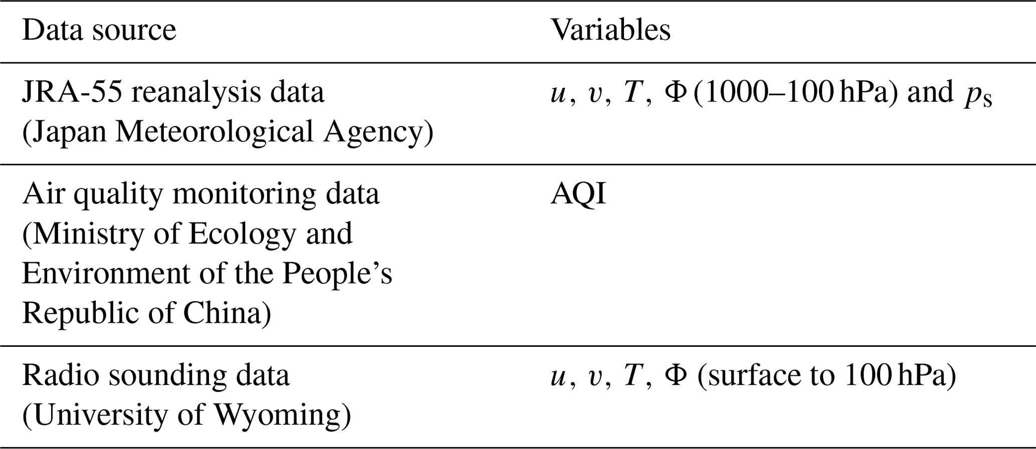
The sounding data obtained from the University of Wyoming provides a direct detection of the atmospheric vertical profile, which would help to explain the changes in AQI observation. The following four sounding stations were selected in NEC: Beijing (39.8^∘ N, 116.5^∘ E), Zhangqiu (36.7^∘ N, 117.6^∘ E), Nanjing (31.9^∘ N, 118.9^∘ E), and Baoshan (31.4^∘ N, 121.5^∘ E). Observation times were 00:00 and 12:00 UTC (08:00 and 20:00 LT). The vertical resolution of the sounding data is comparable to that of JRA-55 model grid reanalysis data. For example, sounding data at Beijing station have 60–70 levels in total and 8–14 levels below 850 hPa during a CAO event on 14–17 December 2016. The data sources of all variables used in this study are listed in Table 1.

Table 1 Data source of variables used in this study. Here, u is zonal winds, v is meridional winds, T is air temperature, Φ is geopotential height, and p_s is surface pressure.

2.2 Isentropic analysis of the cold air outbreak

The identification and quantification of the cold air mass and its outbreaks are performed by an isentropic analysis method. The cold air mass is defined as a layer of air mass below the threshold isentropic surface of θ_T=280 K, which includes most of the equatorward cold air mass flow (Iwasaki et al., 2014). Thus, the depth of the cold air mass (DP; hPa) can be described as the pressure difference between the ground surface (p_s) and the θ_T surface (p(θ_T)) as follows:

$$\begin{array}{}\text{(1)}& \mathrm{DP}=p_{\mathrm{s}}-p\left({\mathit{\theta }}_{\mathrm{T}}\right).\end{array}$$

The horizontal flux of the cold air mass (F, hPa m s⁻¹) is given by the vertical integration of the horizontal wind (v) and the pressure (p), as follows:

$$\begin{array}{}\text{(2)}& F={\int }_{p\left({\mathit{\theta }}_{\mathrm{T}}\right)}^{p_{\mathrm{s}}}v\mathrm{d}p.\end{array}$$

The negative heat content (NHC; K hPa), reflecting the coldness of the cold air mass, is defined as a vertical integration of the potential temperature difference (θ_T−θ) and pressure (p), as follows:

$$\begin{array}{}\text{(3)}& \mathrm{NHC}={\int }_{p\left({\mathit{\theta }}_{\mathrm{T}}\right)}^{p_{\mathrm{s}}}\left({\mathit{\theta }}_{\mathrm{T}}-\mathit{\theta }\right)\mathrm{d}p.\end{array}$$

Based on the above method, the CAO can be identified by the regional mean cold air mass depth. Previous studies showed that the cold air mass depth usually experiences a sharp increase and reaches a relatively high value during the outbreak (Shoji et al., 2014; Liu et al., 2019, 2021). Thus, the CAO in this study is identified when the regional mean cold air mass depth exceeds 166.8 hPa, which is the sum of mean value (77.3 hPa) and standard deviation (89.5 hPa) of the cold air mass depth on all winter days.According to the above criteria, 52 CAOs are identified over eight winters.

The CAO is further divided into three periods. Figure 1 shows the temporal evolution of the cold air mass depth in NEC during a typical CAO in March 2016. The onset of a CAO event, which is the first day when the regional mean cold air mass depth exceeds the threshold (166.8 hPa), is described as day 0. The “during” period of the CAO starts on the onset day (day 0) to the end on the day when the cold air mass depth falls below the threshold (e.g., day +2 in the CAO event plotted in Fig. 1). The period before CAO is defined as the 2 d before the onset day to the onset day (days −2 to 0). The period after CAO, which is also called the decay phase, is defined as the 3 d after the cold air mass depth falls below the threshold (days +2 to +4 in the CAO event plotted in Fig. 1). The period after CAO varies with events, since the end date of the period during the CAO is different in the selected events. It should be noted that the cold air mass in the period after CAO is described as the residual cold air mass in this study.

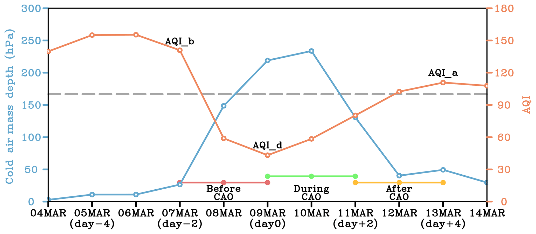
Figure 1 Time series of the regional averaged cold air mass depth (blue line) and AQI (orange line) in NEC (114–122^∘ E, 30–40^∘ N). The gray dashed line denotes the threshold value of the cold air mass depth.

2.3 Measurement of air pollution reappearance and mixing layer height

The description of air pollution reappearance is based on the AQI in different periods of the CAO, as shown in Fig. 1. In the period before CAO, the AQI decreases from a polluted state to a relatively clean state. The AQI usually reaches its minimum in the period during CAO. Then, the AQI increases and results in a new round of air pollution in the period after CAO. Thus, we use the maximum AQI in the period before CAO (AQI_b) and the maximum AQI in the period after CAO (AQI_a) to represent the air pollution before CAO and the reappeared air pollution, respectively. The minimum AQI in the period during CAO (AQI_d) is used to represent the clean state between the air pollution before and after the CAO.

Based on the above analysis, the increase in AQI (IA) is defined as follows to describe the deterioration rate of air pollution in its reappearance:

$$\begin{array}{}\text{(4)}& \mathrm{IA}=\mathrm{AQI}\mathit{\_}a-\mathrm{AQI}\mathit{\_}d.\end{array}$$

A rapid reappearance of air pollution is supposed to have an IA larger than 34.3, which is the standard deviation of the AQI daily variation during the five winters. A reappearance index of air pollution (RI) is also defined below to describe the relative intensity of reappeared air pollution compared to the air pollution before CAO,

$$\begin{array}{}\text{(5)}& \mathrm{RI}=\mathrm{AQI}\mathit{\_}a/\mathrm{AQI}\mathit{\_}b,\end{array}$$

where RI larger (smaller) than 1 denotes that the AQI after CAO is worse (better) than that before CAO.

The mixing layer height is determined from the analysis of the profile of the bulk Richardson number (R_B) using sounding data. The calculation method for R_B is derived from Tang et al. (2016) as follows:

$$\begin{array}{}\text{(6)}& R_{\mathrm{B}}={\displaystyle \frac{g\mathrm{\Delta }\mathit{\theta }\mathrm{\Delta }Z}{\mathit{\theta }\left({\left(\mathrm{\Delta }u\right)}^{\mathrm{2}}+{\left(\mathrm{\Delta }v\right)}^{\mathrm{2}}\right)}},\end{array}$$

where g, θ, Z, u, and v indicate the gravity acceleration, potential temperature, height, zonal wind, and meridional wind, respectively. According to the profiles of R_B and θ, the observations can be separated into a convective state and a stable state. In this study, we found that all the sounding observations are in the stable state with no obvious low-level jet. Therefore, the mixing layer height (MLH) is defined as the altitude at which R_B is greater than 1.

3 Characteristics of air pollution reappearance after CAO

3.1 Statistics of AQI after CAO

To ensure the existence of the rapid reappearance of air pollution after CAO, the relationship of daily changes in AQI and the cold air mass depth is divided into four quadrants in Fig. 2. In winter, 62.1 % of the decrease in the AQI occurs when the cold air mass depth increases, which corresponds to the period before and during the CAO. On the other hand, most of the AQI increase (68.6 %) was accompanied by the cold air mass decrease, which usually occurred in the period after the CAO. Based on these results, the AQI variation changes from decreasing to increasing throughout the CAO, suggesting the existence of air pollution reappearance after the CAO. We also noticed that most of the heavy air pollution was in the quadrant of the cold air mass depth decrease, suggesting that the retreat and dissipation of the cold air mass may be an important meteorological factor for the formation of heavy air pollution.

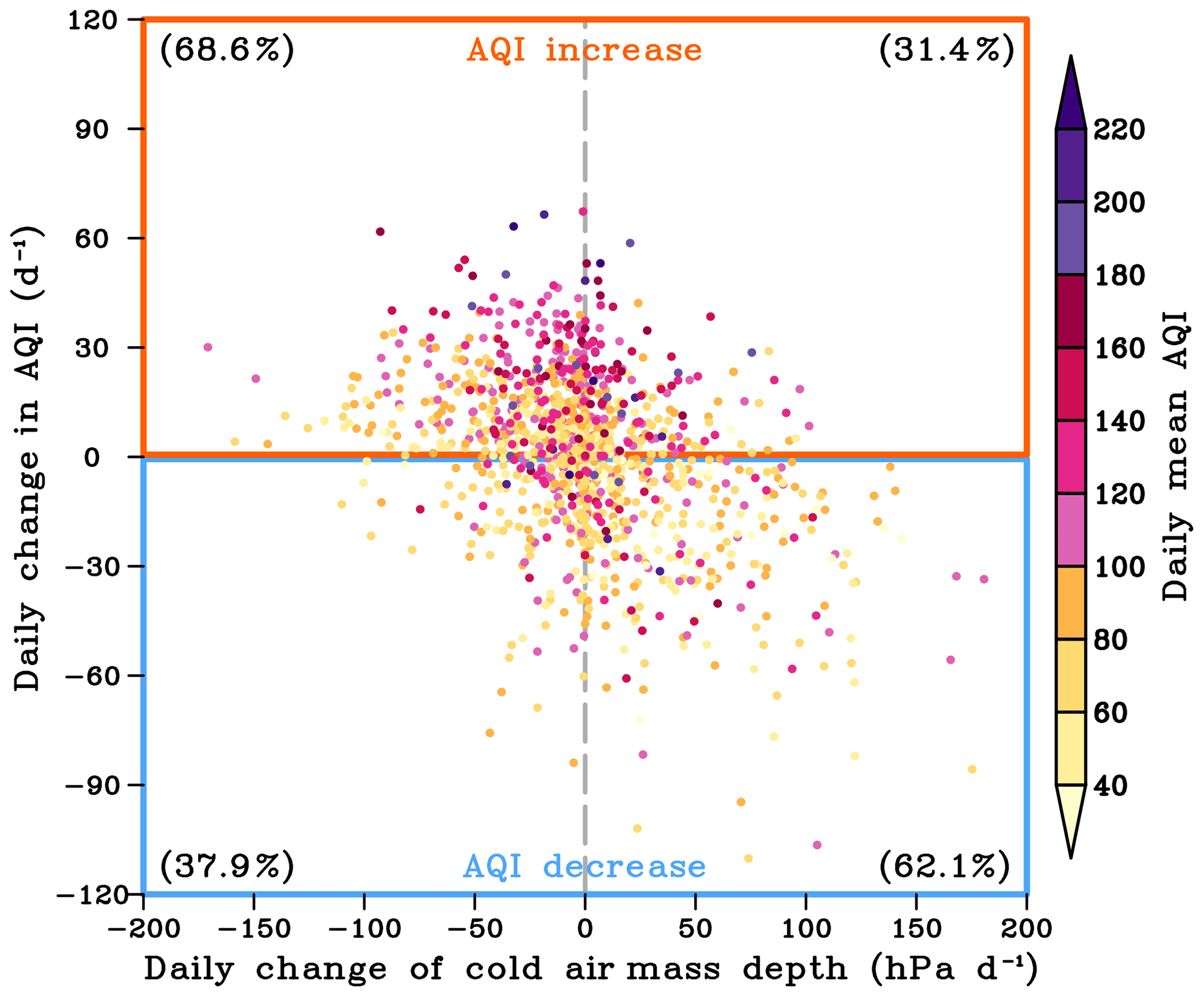
Figure 2 Relationship between the daily changes in the AQI and the cold air mass depth. The daily change is estimated by the current day minus the preceding day. The colors of the dots denote the daily mean cold air mass depth on the current day.

Based on the 52 CAOs selected in this study, the statistical characteristics of the air pollution reappearance after CAO can be demonstrated. Figure 3a compares the AQI daily change rate in the period after CAO to that on all winter days. During the period after CAO, the increase in the AQI has an occurrence frequency of approximately 80 %, which is much higher than that on all winter days (56 %). In particular, the relatively high increase rate (>20 d⁻¹) in the period after CAO has a frequency of approximately twice as high as that on all winter days. Such a frequent rapid increase in the AQI after CAO could induce the reappearance of air pollution and even may result in a worse AQI compared to the AQI before CAO. Using the Eq. (5), Fig. 3b shows the reappearance rate of air pollution (RI) after CAO, whose greater (smaller) value than 1 indicates that the AQI after CAO is worse (better) than the AQI before CAO. Based on the definitions of periods before and after CAO in our study, more than 50 % of the CAOs are found to show a worse AQI after reappearance. In some extreme events, the AQI after CAO could be twice as high as the AQI before CAO. These facts show that, even if the CAO brings several days of clean air, it may lead to a deterioration in the AQI to the polluted or an even worse state.

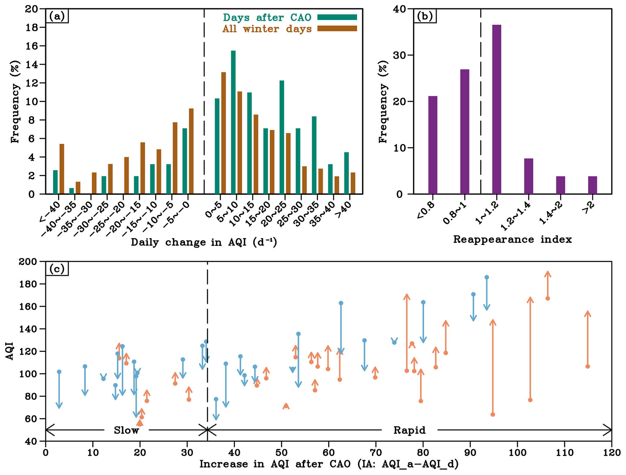
Figure 3 (a) Statistical distribution of the daily change in AQI calculated by all of the days during the eight winters (brown bars) and days during the period after the CAOs (green bars). (b) Statistical distribution of the reappearance index of air pollution in 52 CAO events. (c) The increase in the AQI (x axis) and the change in the AQI from the period before the CAO to the period after CAO (vertical arrows) in 52 CAO events. The black dashed line denotes the standard deviation of AQI. The arrowhead and tail represent AQI_a and AQI_b, respectively. The orange (blue) arrows denote that the AQI worsens (improves) after CAO.

Figure 3c shows that the IA (position of arrows on x axis) in all of the CAO events has a positive value, which means that AQI has experienced an increase after CAO. This result confirms that the reappearance of air pollution is a common phenomenon. Considering the different characteristics of AQI variations after the CAO, the CAOs can be categorized into a “slow reappearance” group and a “rapid reappearance” group, according to IA defined by Eq. (4). Among the 52 CAOs, 19 (36.5 %) show a slow reappearance of air pollution after CAO (CAO_slow), with an increase in the AQI of less than 1 standard deviation of the AQI daily variation (IA ≤34.3). Note that not all CAOs are accompanied by a rapid air pollution reappearance. The remaining 33 CAOs (63.5 %) featured a rapid reappearance of air pollution (CAO_rapid). In Fig. 3c, the arrow on the y axis has a similar meaning to RI, indicating whether the air quality after CAO will become better or worse than that before CAO. The position of the arrowhead and tail on y axis denotes AQI_b and AQI_a, respectively. The orange up-arrow (blue down-arrow) indicates that the reappeared air pollution has a heavier (lighter) degree than the air pollution before CAO. The result shows that most CAO_slow events have a better AQI than that before CAO, while nearly two-thirds of CAO_rapid events face a worse AQI. The above differences in AQI changes after CAO suggest that the air pollution reappears rapidly or slowly may be modulated by the detailed characteristics of CAO.

3.2 Relationship between the reappearance of air pollution and CAO

In terms of spatial averages over NEC, Fig. 4 shows large differences in the cold air mass depth and AQI between CAO_rapid and CAO_slow events. For CAO_rapid events (Fig. 4a), the cold air mass depth increases from day −2 and reaches its maximum on day 0. Then, the cold air mass depth gradually decreases to approximately 100 hPa in the following 3 d. During the whole life cycle of the CAO_rapid event, the AQI shows a reversed variation in the cold air mass depth. From day −2 to day 0, the AQI fell to a moderate level below 70. However, shortly after, the AQI increased rapidly to nearly 130 on day +2, which was worse than the AQI before the CAO. For CAO_slow events (Fig. 4b), the cold air mass depth also increases from day −2 to day 0 and reaches a value similar to that in CAO_rapid events. After day 0, the cold air mass depth drops to the minimum on day +2 at a much faster rate than that in CAO_rapid events and rises again from day +3. During the CAO_slow events, the AQI still varies conversely to the cold air mass depth. However, the decrease in the AQI starts on day 0, which is later than that in CAO_rapid events, and the variation in the AQI also has a relatively small amplitude. Such differences in the removal of air pollution may be associated with the thermal/dynamical features of CAO (Liu et al., 2019). The contrasts of the CAO_rapid and CAO_slow events suggest that there may be two favorable conditions for the rapid air pollution reappearance, i.e., one is the relatively slow decrease in the cold air mass depth, and the other is the longer time period before the next CAO.

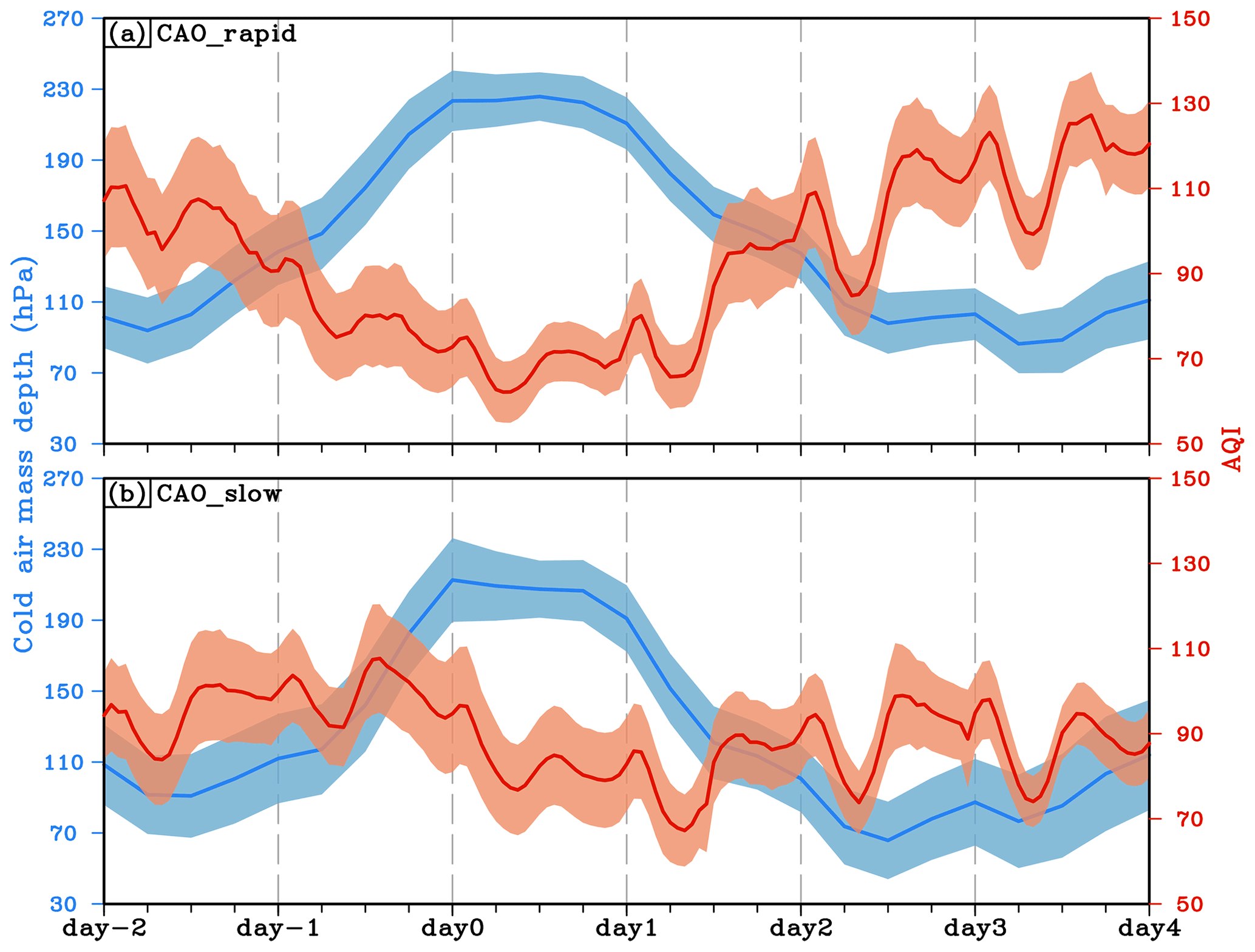
Figure 4 Evolutions of the spatially averaged (NEC at 114–122^∘ E, 30–40^∘ N) cold air mass depth and AQI during CAOs. Panels (a) and (b) are composited by the CAO_rapid events and CAO_slow events, respectively. Blue lines and red lines denote the cold air mass depth and AQI, respectively. Shading represents the 95 % confidence interval of the composited mean value.

We further investigate the spatiotemporal collocation of the AQI and the cold air mass distributions during and after the CAO. For CAO_rapid events, a thick layer of the cold air mass accompanying the strong southeastward flux is observed in NEC on day 0 (Fig. 5a and b). At this stage, the AQI decreased markedly, especially in the eastern part of NEC. From day +1 to day +3, the southeastward flux of the cold air mass weakens, and a quasi-stationary residual cold air mass occupies NEC (Fig. 5c–h). During this period, the AQI increased rapidly and even exceeded 150 (middle level air pollution) at a number of stations. The worst AQI usually occurs in the region with a cold air mass depth of 50–150 hPa. For CAO_slow events on day 0, the cold air mass depth has a distribution similar to that in CAO_rapid events (Fig. 6a and b). However, the cold air mass fluxes in CAO_slow events contain a larger eastward component than those in CAO_rapid events. Such an enhanced eastward flux leads to the quick eastward retreat of the residual cold air mass on days +1 and +2 (Fig. 6c–f). During this period, an increase in the AQI is also observed in the area covered by the residual cold air mass. On day +3, the cold air mass enhances again in the northern part of NEC and thus ends the reappearance of air pollution (Fig. 6g and h). According to the above results, we found that the reappearance of air pollution tends to occur in the residual cold air mass with nearly no horizontal flux during the decay period of the CAO.

Figure 5 Spatial distributions of the composited cold air mass depth (shaded), horizontal fluxes of the cold air mass (black vectors), and AQI (colored dots) during CAO_rapid events. The black boxes denote the NEC (114–122^∘ E, 30–40^∘ N).

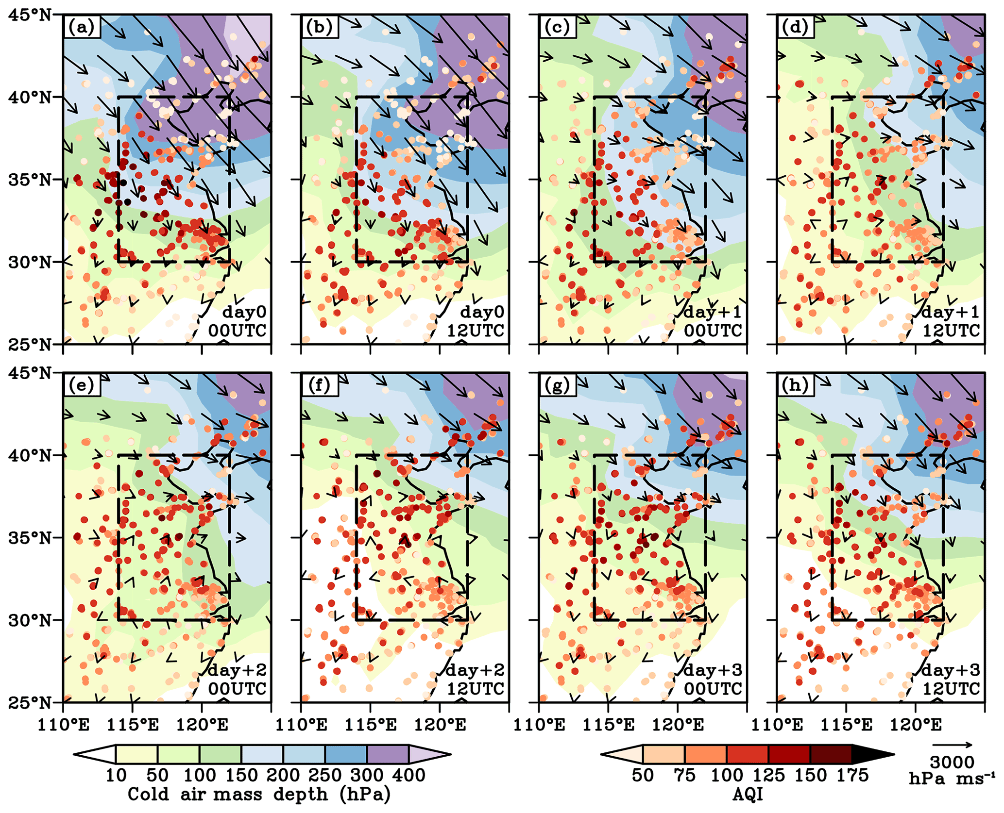
Figure 6 The same as Fig. 5 but composited by the CAO_slow events.

4 Factors affecting the rapid reappearance of air pollution

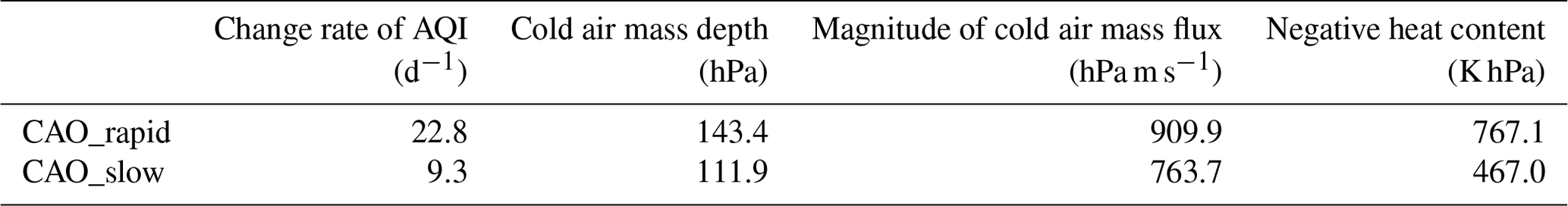
To determine the dominant feature of CAO controlling the reappearance of air pollution, Table 2 compares the dynamic and thermodynamic properties of the cold air mass in CAO_rapid and CAO_slow events. The cold air mass properties are averaged in the period from day +1 to +2, which corresponds to the rapid increase period of the AQI in Fig. 4. The results reveal that the magnitude of the cold air mass flux shows a relatively small difference between the two types of CAO. However, large differences exist in the depth and NHC of the cold air mass, which may be the key factors affecting the air pollution reappearance. The cold air mass in CAO_rapid events (143.4 hPa and 767.1 K hPa) is thicker and colder than that in CAO_slow events (111.9 hPa and 467.0 K hPa). To explore how the depth and NHC of the cold air mass modulate the air pollution reappearance, a CAO_rapid event (14–17 December 2016) and a CAO_slow event (11–14 February 2018) are selected for further analysis.

Table 2 Averaged AQI change rate and the cold air mass properties during the period from day +1 to +2.

4.1 Cold air mass depth

Figures 7 and 8 examine the profile of potential temperatures below 3 km at the four stations (see Sect. 2.1) under the effect of the CAO. During the CAO_rapid event on day 0, the lapse rate of potential temperature is small from the near-ground level to the height of approximately 1.5 km (Fig. 7a). Above the height of 1.5 km, the lapse rate suddenly increases, forming an air layer with a large vertical gradient of potential temperatures. Such a large vertical gradient of potential temperature denotes a strong stable stratification, weakening the vertical mixing of air pollutants to the upper level. In the case of high emissions in NEC (Zhang et al., 2012; Gao et al., 2016), atmospheric conditions such as these are favorable for the accumulation of air pollutants in the near-surface atmosphere (Zhang et al., 2022). On the other hand, the large gradient layer can be recognized as the upper boundary of the cold air mass since the cold air mass features strong thermal contrast to its surroundings. This upper boundary of the cold air mass acts as a lid confining the air pollutant in the residual cold air mass. Previous studies also show that air pollutants usually increase and are trapped in the residual cold air mass during the period after CAO (Kang et al., 2019; Liu et al., 2019). From day 0 to +1, the height of the large gradient layer is maintained at approximately 1.5 km, and then it slowly drops to 0.5 km in the following 2 d. Such a temporal evolution is highly consistent with the evolution of the cold air mass depth (Fig 7a and b). In the same period, the AQI increases nearly 2 times from 50 to 150.

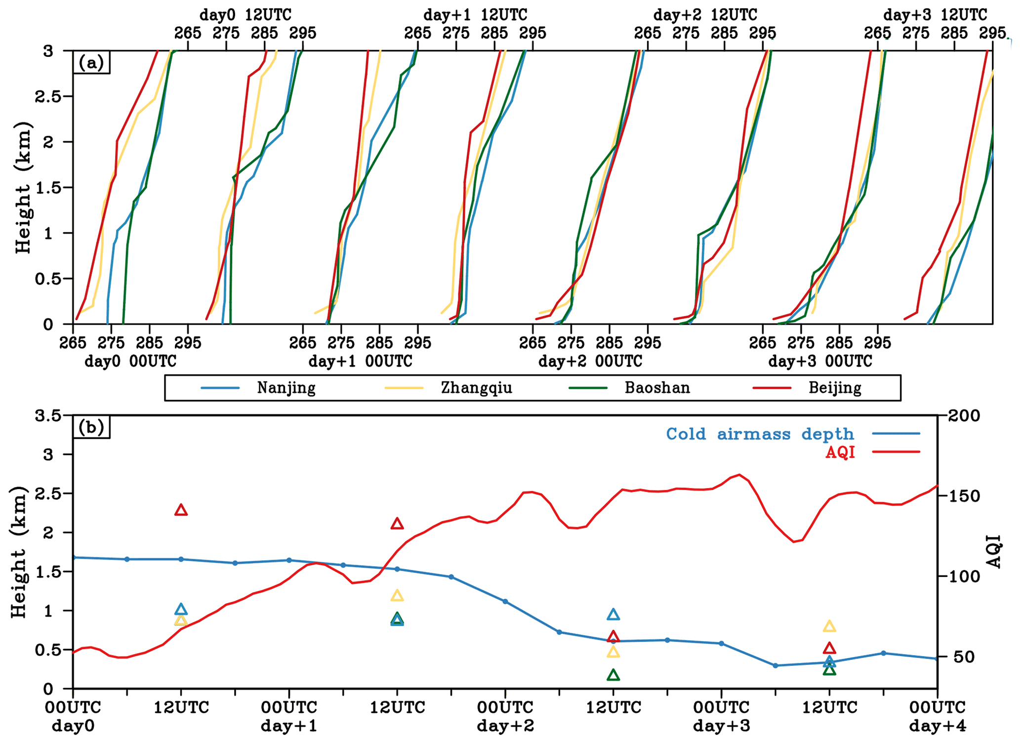
Figure 7 (a) Vertical profiles of potential temperature at four stations (from north to south are Beijing, Zhangqiu, Nanjing, and Baoshan) during a CAO rapid event from 14 to 17 December 2016. (b) Time series of the regional averaged cold air mass depth and the AQI in NEC and MLH (colored triangles) at four stations during a CAO_rapid event from 14 to 17 December 2016.

Figure 8 The same as Fig. 7 but during a CAO_slow event from 11 to 14 February 2018.

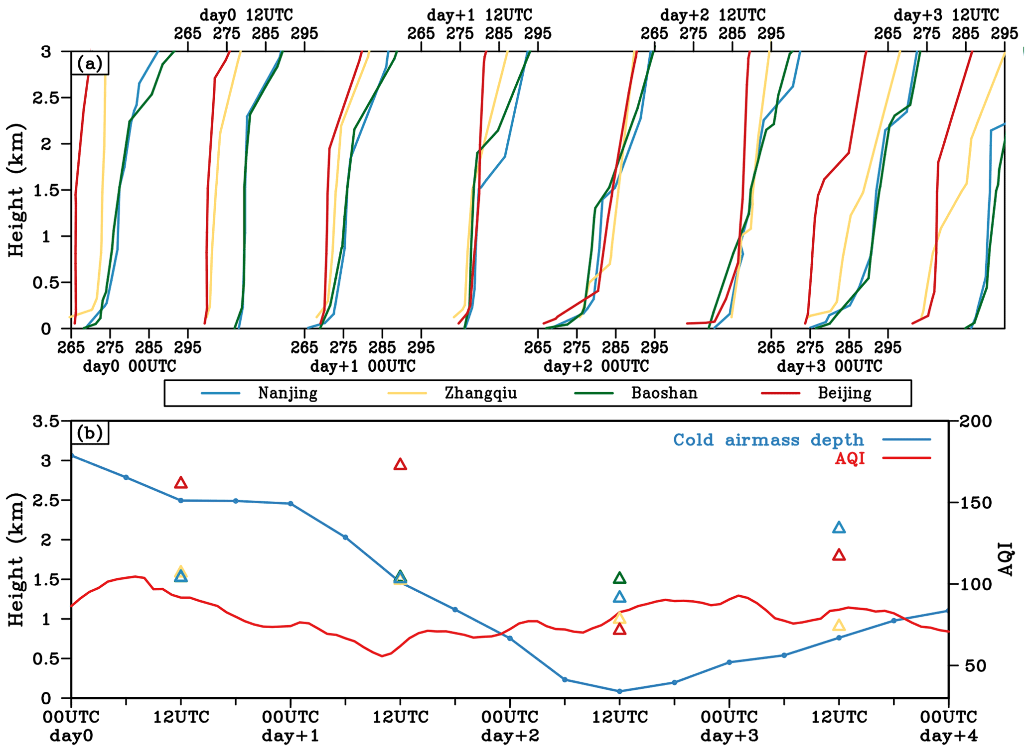
The low-level atmosphere with a small lapse rate of potential temperature in Fig. 7a may represent the mixing layer (or boundary layer), featuring convection, vertical mixing, and dry adiabatic lapse rates. The mixing layer could greatly impact the accumulation and dissipation of air pollutants (Holzworth, 1967; Tang et al., 2016). Many studies have reported that the MLH is a good indicator of air quality (Su et al., 2018; Gui et al., 2019). However, the calculation of MLH is somewhat complex (Eq. 6), and the MLH calculated by most mainstream reanalysis datasets has obvious bias compared to the sounding data (Guo et al., 2021). Figure 7b shows the MLH at the four stations at 12:00 UTC. The MLH and cold air mass depth have good agreement in both values and temporal variations. This is because the vertical structures of temperature and wind in the low-level atmosphere are mainly forced by the cold air mass during CAO. Thus, the residual cold air mass happens to be the mixing layer and modulates the evolution of the AQI. In addition, the calculation of the cold air mass depth using reanalysis data is much easier than the calculation of MLH using sounding or other observation data, suggesting that the cold air mass depth may be a good substitute for MLH in periods during and after the CAO.

In the CAO_slow event on day 0, the potential temperature has a profile similar to that in the CAO_rapid event (Fig. 8a). The large gradient layer is located at approximately 2.5 km, which corresponds to the cold air mass depth and MLH (Fig. 8b). Such features in the cold air mass and atmospheric stratification continue to 00:00 UTC on day +1. During this period, the AQI shows no increase due to the high MLH. From days +1 to +2, the cold air mass depth decreases rapidly and almost disappears in the southern part of NEC, leading to the disappearance of the large gradient layer in the low troposphere. It should be noted that the mixing layer at this time is not forced by the residual cold air mass since it is absence. As the MLH decreases to 1.5 km, the AQI experiences a relatively slow increase. On day +3, the cold air mass depth increases again, causing an increase in the MLH and a decrease in the AQI.

Based on the analyses of a CAO_rapid event and a CAO_slow event, we conclude that the intrusion of cold air mass forces the lower troposphere into a stable stratification that is favorable for the increase in the AQI. Thus, the depth and persistence of the residual cold air mass were thought to be two factors that influence the deterioration rate of air pollution. It is clear that a longer persistence of the residual cold air mass is favorable for the rapid reappearance of air pollution, while the relation between the cold air mass depth and the AQI increase rate is quite complex. Regarding the rapid reappearance of air pollution, the cold air mass depth is not the lower the better. In CAO_rapid events, for example (Fig. 5), the increase in the AQI is less obvious in the region to the south of NEC (25–30^∘ N) with a cold air mass depth thinner than 100 hPa. Moreover, the AQI increase rate will not vary monotonically with the cold air mass depth. The AQIs in the Yangtze River Delta (30–32^∘ N, 118–122^∘ E) and Bohai Rim (37–40^∘ N, 117–122^∘ E) have similar increase rates, although the Bohai Rim has a cold air mass depth much thicker than that of the Yangtze River Delta. Similar results can also be found in CAO_slow events (Fig. 6). According to these analyses, Fig. 9 presents the relation between the cold air mass depth and the AQI change rate. With the increasing cold air mass depth, the change rate of the AQI first increases and then slightly decreases. A cold air mass depth that is too thick dilutes the surface air pollutant concentration, but a cold air mass depth that is too thin damages the persistence of the cold air mass. The cold air mass depth in a moderate range of 150–180 hPa (approximately 1.5–1.8 km) is most favorable for the air pollution reappearance, with a mean increase rate of 26.1 d⁻¹. In some extreme cases exceeding the 90th percentile, the AQI increase rate can reach 72.5 d⁻¹.

Figure 9 Distribution of the change rate of the AQI with the cold air mass depth during the period after the CAO.

4.2 NHC and vertical thermal structure

As another key factor revealed in Table 2, NHC also contributes to air pollution reappearance. According to the definition in Sect. 2.2 (Eq. 3), NHC is proportional to the production of the cold air mass depth (DP) and vertical averaged potential temperature difference $\left(\mathrm{\Delta }\mathit{\theta }=\stackrel{\mathrm{‾}}{({\mathit{\theta }}_{\mathrm{T}}-\mathit{\theta })}\right)$. If the potential temperature increases linearly with height, Δθ can be further simplified as (θ_T−θ_s), where θ_s is the surface potential temperature. Here, diving the NHC by (DP)² lead us to the following:

$$\begin{array}{}\text{(7)}& {\displaystyle \frac{\mathrm{NHC}}{{\left(\mathrm{DP}\right)}^{\mathrm{2}}}}\propto {\left.{\displaystyle \frac{\mathrm{\Delta }\mathit{\theta }}{\mathrm{\Delta }p}}\right|}_{\mathrm{cold}\mathrm{airmass},}\end{array}$$

where Δp is equal to DP when referring to the cold air mass, and $\frac{\mathrm{\Delta }\mathit{\theta }}{\mathrm{\Delta }p}$ indicates the averaged vertical stability in the cold air mass. Thus, at a given cold air mass depth (DP), a larger NHC will likely result in a more stable stratification, which is favorable for air pollution reappearance. This explains why the NHC is much larger during the decay period in CAO_rapid events than in CAO_slow events (Table 2). On the other hand, the persistence of the cold air mass will also benefit from the large NHC, which helps to dampen the reduction effect of diabatic heating.

In addition to NHC, the two selected CAO events show that the vertical thermal structure of the cold air mass also influences the stability of low-level troposphere (Fig. 10). On the onset day of the CAO_rapid event (Fig. 10a), the upper boundary of the cold air mass is relatively flat, rising from 900 hPa at 30^∘ N to 770 hPa at 40^∘ N. Inside the cold air mass, the isentropes represented by the potential temperature anomaly are essentially parallel to the upper boundary of the cold air mass. Such flat distributions indicate that the vertical gradient is the dominant component of the potential temperature gradient. As a result, a strong stable layer forms at the upper part of the cold air mass spanning 900–700 hPa. Note that this large vertical gradient layer can also be seen in Fig. 7a. After the outbreak on day +1 (Fig. 10b), the upper boundary of the cold air mass remained almost unchanged, and the negative anomaly of potential temperature weakened slightly. The stable layer still exists at the upper part of the cold air mass, although its intensity is weaker than that on day 0. For the CAO_slow event on day 0 (Fig. 10c), the upper boundary of the cold air mass steeply increases from 900 hPa at 30^∘ N to higher than 600 hPa at 40^∘ N. The slope of the cold air mass in the CAO_slow event is more than twice that in the CAO_rapid event. The isentropes in the cold air mass are almost perpendicular below 850 hPa. In this scenario, the vertical gradient of potential temperature is small in the CAO_slow event, even if it has a thicker and colder cold air mass than that in the CAO_rapid event. Accordingly, a stable layer with smaller intensity but higher altitude (800–600 hPa) is observed over the central and southern parts of the cold air mass. On day +1 (Fig. 10d), the cold air mass depth decreases markedly; however, the slope of isentropes remains large. As a result, the relatively weak stable layer lowers to approximately 850 hPa.

Figure 10 (a, b) Longitude vertical sections of the potential temperature anomaly (colored shading) and vertical gradient of the potential temperature (contour; 10⁻³ K m⁻¹; dotted for $>\mathrm{6}\times {\mathrm{10}}^{-\mathrm{3}}$ K m⁻¹) along 119^∘ E during the CAO_rapid event from 14 to 17 December 2016. The thick black line denotes the upper boundary of the cold air mass. The purple bars denote the mean zonal wind speed in the cold air mass. Panels (c) and (d) are the same as panels (a) and (b) but during the CAO_slow event from 11 to 14 February 2018.

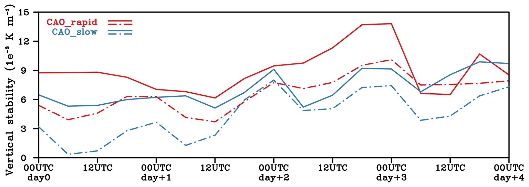
Figure 11 Evolution of spatially averaged (NEC; 114–122^∘ E, 30–40^∘ N) vertical stability at the upper boundary of the cold air mass (solid line) and the averaged vertical stability in the cold air mass (dash dot line) during a CAO_rapid event from 14 to 17 December 2016 (red) and a CAO_slow event from 11 to 14 February 2018 (blue).

The differences in vertical atmospheric stability may lead to different increase rates of AQI during air pollution reappearance. Figure 11 compares the evolutions of vertical stability in NEC during the two CAO events. From 00:00 UTC on day 0 to 12:00 UTC on day +1, the CAO_rapid event has a larger stability than that in the CAO_slow event at both the upper boundary and the entire cold air mass. In particular, the stability of the entire cold air mass in the CAO_rapid event is twice as high as that in the CAO_slow event. During this period, the AQI in the CAO_rapid event increases drastically from 50 to 120 under strong stable stratification, while the AQI in the CAO_slow event remains in the range of 80–100 under weak stable stratification (Figs. 7b and 8b). After 12:00 UTC day +1, the variation in the AQI becomes steady, while the atmospheric stability starts to increase (Fig. 11). This may be attributed to the radiative feedback of the air pollutant (Petäjä et al., 2016; Ding et al., 2016). By comparing the two types of CAO events, we find that the NHC and vertical structure of the cold air mass jointly affect the low-level vertical stability, which modulates the air pollution reappearance. A cold air mass with a small slope of isentropes and a large NHC is favorable for the rapid reappearance of air pollution.

4.3 Impacts of cold air mass features on air pollution reappearance in numerical simulation

To verify the roles of the abovementioned cold air mass features on air pollution reappearance inferred from the analyses of two selected CAO events, numerical experiments using WRF-Chem (Weather Research and Forecasting model coupled with Chemistry) version 4.3 are carried out in this section. The domain of the simulations is designed with a horizontal grid spacing of 10 km, covering most part of East Asia (figure omitted). The FNL (final) data are used as the initial and lateral boundary conditions to drive the meteorological simulation. The MEIC (Multiresolution Emission Inventory for China) anthropogenic emission inventories are used in the chemical simulation. The main physical and chemical parameterization schemes include the WSM6 microphysics, the Mellor–Yamada–Janjic (MYJ) planetary boundary layer (PBL) scheme, the Rapid Radiative Transfer Model (RRTM) for longwave and shortwave radiation, and RADM2-MADE/SORGAM (Regional Acid Deposition Model version 2–Modal Aerosol Dynamic for Europe/Secondary Organic Aerosol Model) for gas-phase chemical and aerosol schemes.

Figure 12 shows the spatial averaged cold air mass depth, boundary layer height, vertical stability, and surface PM_2.5 concentration during the CAO_rapid and CAO_slow events. The emissions in both experiments are set as the same values in December 2016 to investigate the impacts of meteorological conditions. In the experiment of CAO_rapid event, the air pollutant concentration increases rapidly on days 0 and +1 under the condition of the relatively low boundary layer height and strong vertical stability. Such conditions of the atmospheric boundary layer are not conducive to the diffusion of air pollutants and tend to induce rapid reappearance of air pollution (Zhang et al., 2014; Liu et al., 2017). In the CAO_slow experiment, however, the PM_2.5 concentration keeps in a low level due to the relatively high boundary layer height and weak vertical stability. In addition, the temporal evolutions of these variables are highly consistent with the observations shown in Figs. 7, 8, and 11, suggesting that both the rapid and slow reappearances of air pollution can be well captured by the numerical model.

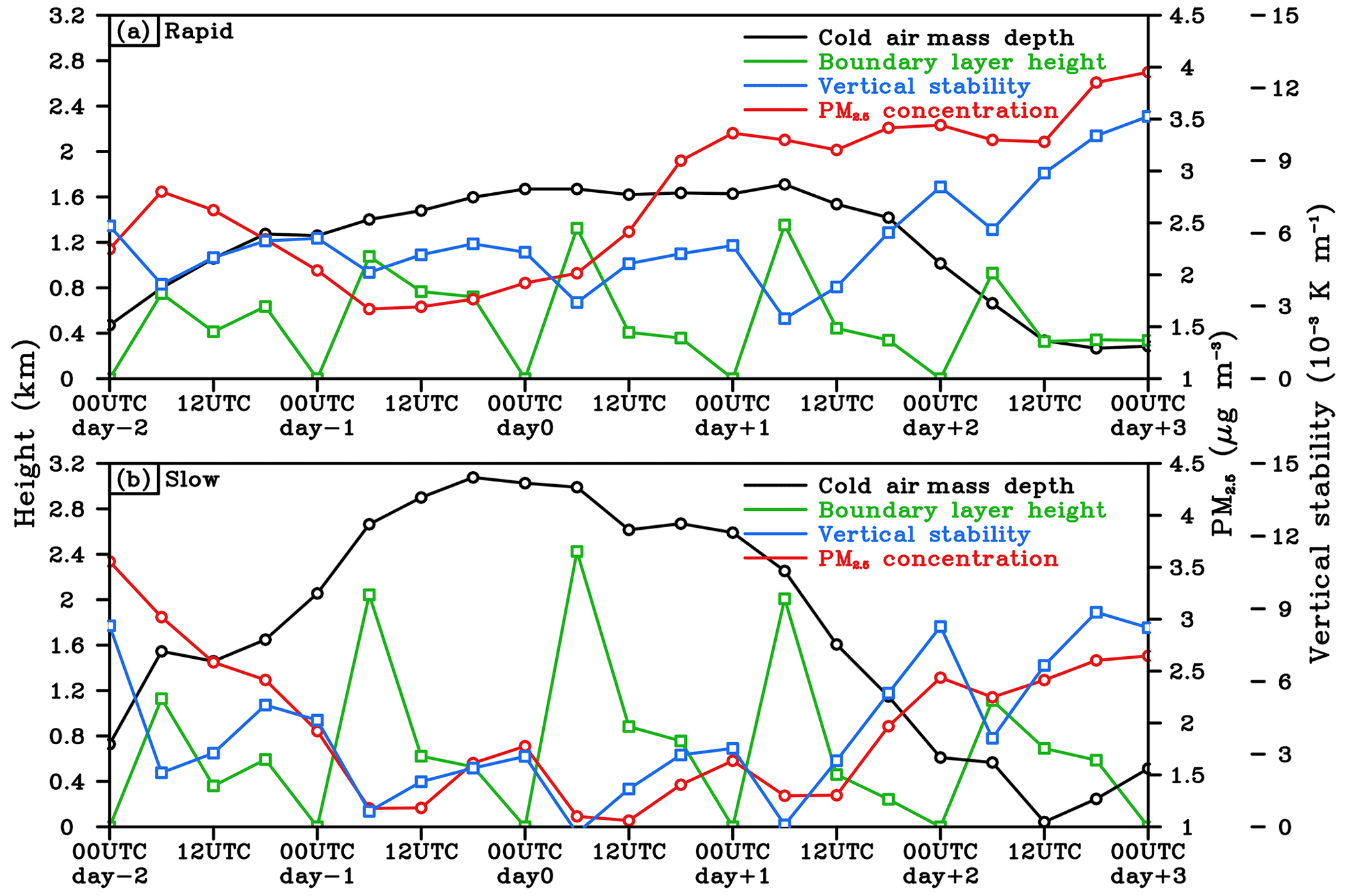
Figure 12 Evolution of the spatially averaged (NEC; 114–122^∘ E, 30–40^∘ N) cold air mass depth, atmospheric boundary layer height, vertical stability (1000–850 hPa), and surface PM_2.5 concentration during (a) CAO_rapid event from 14 to 17 December 2016 and (b) CAO_slow event from 11 to 14 February 2018.

Table 3 Averaged cold air mass properties and atmospheric boundary layer conditions on day 0 from control and sensitive experiments. Upward (downward) arrows denote that the value of sensitive experiment is greater (less) than the value in control experiment.

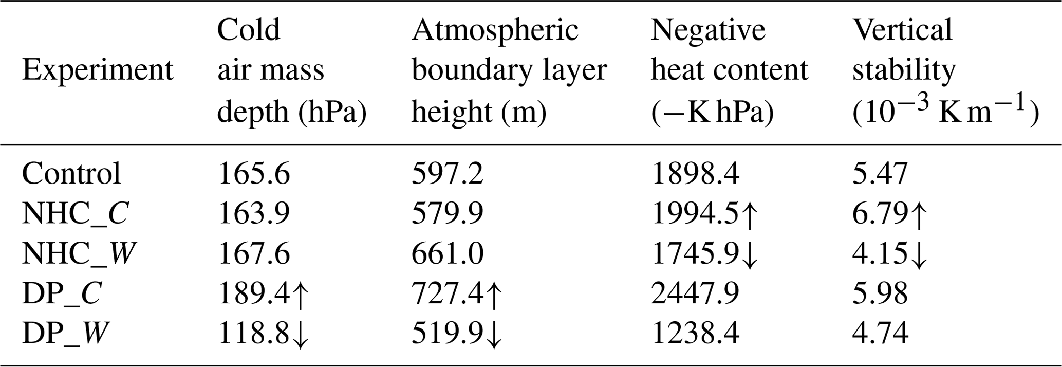
To further verify the connection between the cold air mass properties and the boundary layer diffusion conditions, as discussed in Sect. 4.1 and 4.2, a control experiment (the CAO_rapid event from 14 to 17 December 2016) and additional sensitive simulations are also conducted. In the sensitive experiments, temperature disturbances are artificially added in the initial field, following Bai et al. (2019). In the NHC_C (NHC_W) experiment, the NHC of the cold air mass is increased (decreased) by adding a cold (warm) bubble centered at a height of 0 km. The cold (warm) bubble has a latitudinal radius of 10 km, longitudinal radius of 5 km, and a vertical radius of 2 km, with a minimum potential temperature perturbation of −8 (8) K. The temperature disturbance, in a cold bubble, for example, is minimized at the center and increases to 0 K following a cosine function over the horizontal and vertical radius. To increase (decrease) the cold air mass depth in the DP_C (DP_W)_C experiment, the cold (warm) bubble added in the initial field moves to the height of 2 km. Note that the NHC may also change with the cold air mass depth in DP_C and DP_W experiments.

Table 3 shows the simulation results averaged in the study area on day 0, when air pollutant has the most rapid increase rate as shown by Fig. 12a. In NHC_C and NHC_W experiments, changes in NHC cannot cause an obvious variation in boundary layer height but can lead to changes in vertical stability. In DP_C and DP_W experiments, despite the changes in NHC and vertical stability, we find that changes in the cold air mass depth will result in obvious changes in boundary layer height. These sensitive experiments confirm the main results of Sect. 4.1 and 4.2; that is, the properties of CAO could effectively impact the diffusion conditions in atmospheric boundary layer.

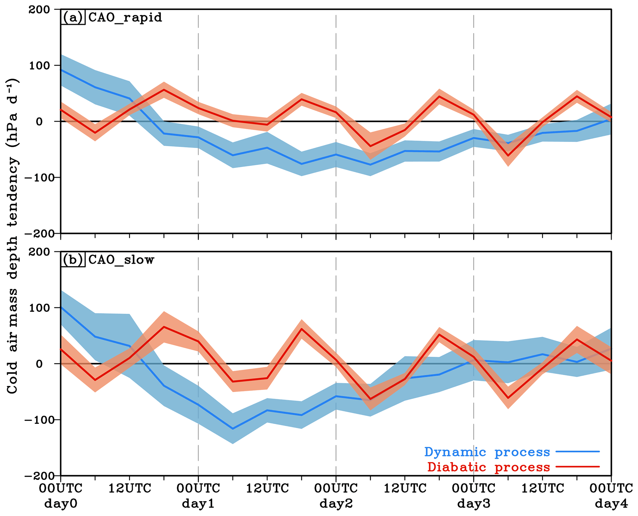
Figure 13 Evolution of the spatially averaged (NEC; 114–122^∘ E, 30–40^∘ N) cold air mass depth tendency during CAOs. Blue and red lines denote the contributions of the dynamic and diabatic processes to the tendency of cold air mass depth, respectively. Panels (a) and (b) are composited by the CAO_rapid events and CAO_slow events, respectively. Shading represents the 95 % confidence interval of the composited mean value.

4.4 Possible mechanisms governing key features of cold air mass

Since the properties of the residual cold air mass control the features of air pollution reappearance, it is necessary to investigate the possible mechanisms modifying cold air mass changes during the decay period of the CAO. According to Iwasaki et al. (2014), the total cold air mass conservation equation can be described as follows:

$$\begin{array}{}\text{(8)}& {\displaystyle \frac{\partial \mathrm{DP}}{\partial t}}=-\mathrm{\nabla }\cdot {\int }_{p\left({\mathit{\theta }}_{\mathrm{T}}\right)}^{p_{\mathrm{s}}}v\mathrm{d}p+G\left({\mathit{\theta }}_{\mathrm{T}}\right).\end{array}$$

The change in the cold air mass depth is caused by the horizontal convergence/divergence of the cold air mass flux ($-\mathrm{\nabla }\cdot {\int }_{p\left({\mathit{\theta }}_{\mathrm{T}}\right)}^{p_{\mathrm{s}}}v\mathrm{d}p)$ and the vertical flux crossing the θ_T surface (G(θ_T)). The former represents the dynamic process, and the latter is related to diabatic cooling and heating.

Based on Eq. (8), Fig. 13 compares the composited evolutions of the cold air mass changes induced by dynamic and diabatic processes. During the CAO_rapid events (Fig. 13a), the decrease in the cold air mass is mainly attributed to the dynamic process, which has shown a decreasing effect since 18:00 UTC day 0 and reaches a maximum of −75.9 hPa d⁻¹ at 18:00 UTC day +1. The effect of the diabatic process on the cold air mass exhibits an obvious diurnal variation, cooling/increasing the cold air mass at night (12:00–24:00 UTC) and heating/decreasing the cold air mass during the daytime (00:00–12:00 UTC). On days 0 and +1, the diabatic heating is weak during the daytime, inducing a slight net increase in the cold air mass caused by the diabatic process. From day +2, the heating effect intensifies and reduces the cold air mass jointly with the dynamic process. During the decaying period of cold air mass on days +1 and +2, the average effects of dynamic and diabatic processes on cold air mass are −56.9 and 7.4 hPa d⁻¹, respectively.

For CAO_slow events (Fig 13b), the dynamic process still dominates in the cold air mass decrease. The average tendencies of the dynamic and diabatic processes on days +1 and +2 are −66.7 and 1.5 hPa d⁻¹, respectively. The two types of processes show similar variations but larger amplitudes compared to those in CAO_rapid events. For the effect of the diabatic process, a much stronger diurnal variation is observed. This may be related to the relatively small potential temperature lapse rate and NHC in CAO_slow events (Fig. 11 and Table 2). Strong diabatic heating also shows a notable contribution to the cold air mass reduction during the daytime, although the daily average effect of the diabatic process is relatively small. For the decrease in cold air mass associated with the dynamic process, the decreasing rate in CAO_slow events could reach a maximum rate of −116.0 hPa d⁻¹, which is 52.8 % higher than that in CAO_rapid events. This enhanced contribution of the dynamic process can be related to the strong easterlies in the cold air mass, which are illustrated in the bar charts of Fig. 10. The strong eastward transport from NEC to the marine area quickly reduced the cold air mass depth in the CAO_slow events.

5 Discussion: large-scale circulation pattern of the CAO associated with the rapid reappearance of air pollution

In this section, we further check the large-scale circulation pattern of the CAO to see if we can find precursors for rapid air pollution reappearance. Figure 14 shows the composited spatial evolutions of the cold air mass depth and flux during the initial stages (days −4 to 0) of CAO_rapid and CAO_slow events. For CAO_rapid events (Fig. 14a), an anticyclonic pattern of an anomalous cold air mass flux appears in northern Siberia (60–80^∘ N, 70–120^∘ E) on day −4. To the south of this anomalous anticyclone, near Lake Baikal, the cold air mass depth shows a positive anomaly. In the following 2 d, the anticyclone intensifies in strength and extends from the high latitudes to the middle latitudes, covering most of Siberia. The strong southward flux of cold air mass on the eastern flank of the anticyclone induces an increase in the cold air mass depth and guides the cold air mass to move southeastward. From day −1 to day 0, the anticyclonic pattern gradually disappears, while the strong southward flux on its eastern flank is strengthened and extends further south. Driven by this southward cold air mass flux, the cold air mass depth anomaly dominates NEC.

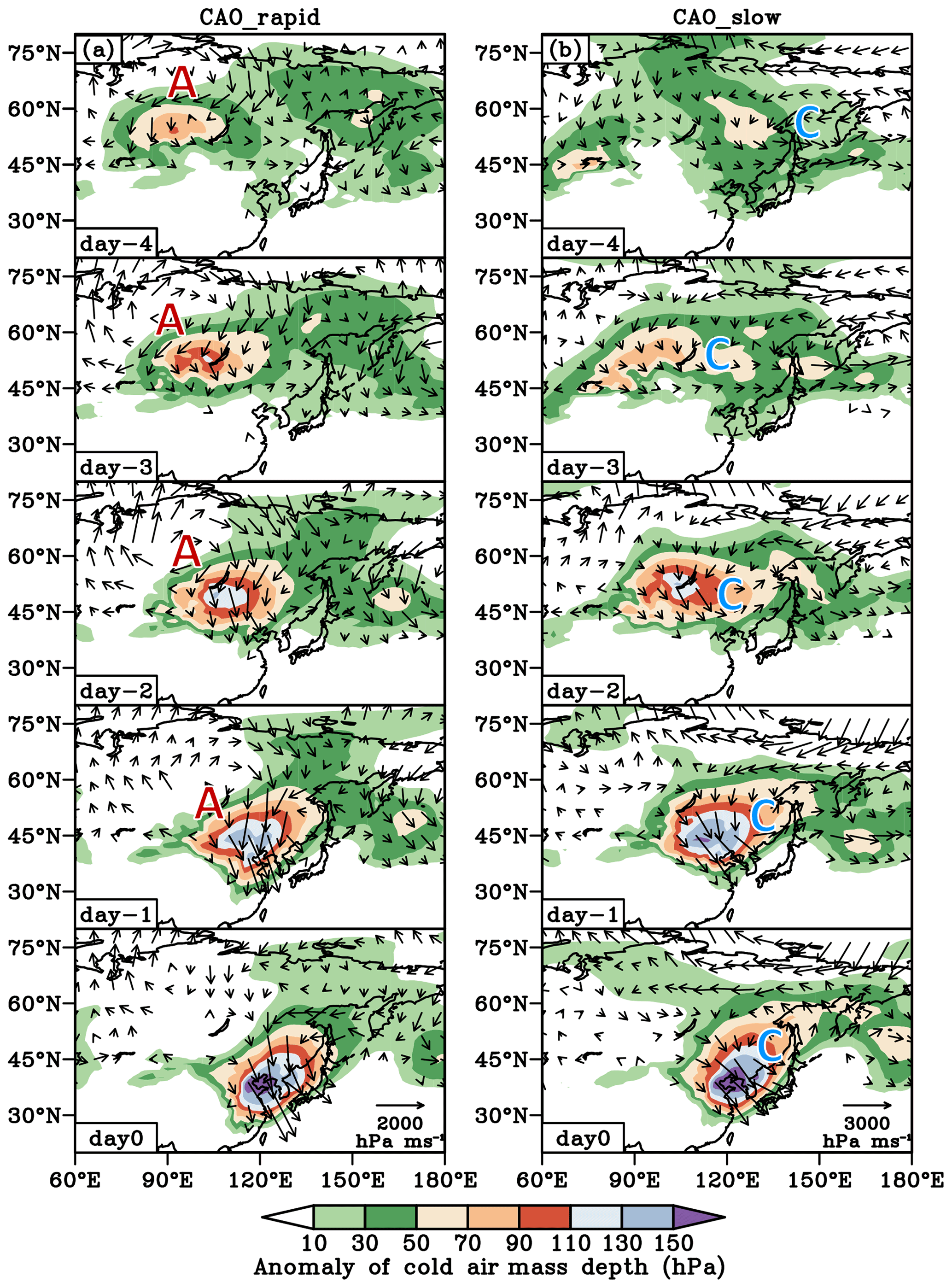
Figure 14 Large-scale anomalies of cold air mass depth (shading) and cold air mass flux (vectors) in the initial stage from day −4 to 0. Panels (a) and (b) are composited by the CAO_rapid events and CAO_slow events, respectively.

The CAO_slow events have distinct features in their circulation patterns that are different from CAO_rapid events (Fig. 14b). On day −4, a cyclonic pattern of anomalous cold air mass flux is observed in northeastern Asia, which is also featured by the positive anomaly of cold air mass depth. Meanwhile, a southward flux of cold air mass with cyclonic curvature can be found to the northwest of Lake Baikal (55–70^∘ N, 80–100^∘ E). During days −3 and −2, the cyclonic pattern and the corresponding cold air mass depth anomaly over northeastern Asia weakens and moves to the northwestern Pacific. The southward cold air mass flux near Lake Baikal intensifies rapidly and forms a new cyclonic pattern in northeastern Asia. Along with the strengthening of the new cyclonic pattern, a positive anomaly of cold air mass depth occurs and increases rapidly. In the following days, the newly formed cyclonic pattern and anomalous cold air mass depth continued to intensify and be swept into NEC.

The above results suggest that CAO_rapid and CAO_slow events are distinguished by the dominant pattern of large-scale anomalous cold air mass flux in the early period of the CAO (days −4 to −2). The CAO_rapid events feature an anticyclonic pattern in northern Siberia, while CAO_slow events are dominated by a cyclonic pattern in northeastern Asia (Fig. 13). The circulation patterns of CAO_rapid and CAO_slow events are also reported as the two main types of CAOs in East Asia, which account for 27 % and 26 % of the total frequency, respectively (Liu et al., 2021). Such differences in large-scale circulation patterns have a close association with the evolution of the cold air mass after CAO. For CAO_rapid events, the southward flux at the eastern flank of the anticyclone is favorable for the maintenance of cold air mass in NEC (Figs. 5, 13a, and 14a). For CAO_slow events, however, the cold air mass flux at the southern flank of the cyclone contains a large eastward component, causing a fast departure of cold air mass from NEC (Figs. 6, 13b, and 14b). Therefore, the anticyclonic and cyclonic patterns in high-latitude Eurasia can be used as precursors for the estimation of air pollution reappearance after the CAO.

6 Conclusions

The CAO is well known to have a strong removal effect on air pollution over NEC. However, air pollution may experience a rapid reappearance after the CAO and even lead to worse pollution. Based on the AQI measurement and quantitative description of cold air mass during the last eight winters, the detailed characteristics and possible causes of air pollution reappearance after 52 CAOs are analyzed. During the period after the CAO, the increase in the AQI in NEC has a probability of more than 80 %, and the AQI increase rate is much faster than that in other periods in winter. In more than half of the CAOs, the AQI in the reappeared air pollution is worse than the AQI before CAO. The CAOs are divided into a rapid reappearance group (63.5 %) and a slow reappearance group (36.5 %) by the increase rate in the AQI. CAO_rapid events tend to have a relatively slow decrease in the cold air mass depth and a long interval time before the next CAO. Spatiotemporal evolution shows that the reappearance of air pollution usually occurs in the first 2 d after CAO. The region of the worst AQI after the air pollution reappearance features a slowly decreasing residual cold air mass with nearly no horizontal flux.

The rapid reappearance of air pollution is mainly attributed to the stable stratification in the lower troposphere forced by the intrusion of a cold air mass. A comparison of the two groups of CAOs shows that the depth, NHC, and the vertical structure of the cold air mass are key features modulating the reappearance of air pollution. The cold air mass depth could well present the MLH and has good agreement with the MLH in both value and variation. A moderate depth (150–180 hPa) of the cold air mass is most favorable for air pollution reappearance since it is thin enough to restrict the spread of air pollutants and thick enough to maintain its own existence. The NHC is proportional to the vertical stability and persistence of the cold air mass. For a fixed cold air mass depth, a larger NHC will lead to a more rapid reappearance of air pollution. The vertical structure, represented by the slope of isentropes, in the cold air mass could also influence the low-level vertical stability. The cold air mass with relatively flat isentropes will likely have a large vertical component of the potential temperature gradient, which is conducive to the reappearance of air pollution.

Further analysis shows that the evolution of the residual cold air mass and the above conditions are mainly associated with the dynamic process rather than diabatic heating/cooling. The strength of the eastward cold air mass flux after CAO is an important factor affecting the decreasing rate of the residual cold air mass. This study also investigates the possible indication of a large-scale circulation pattern of the CAO during its initial stage in estimating the reappearance of air pollution after CAO. The CAOs driven by the circulation of anticyclonic pattern in northern Siberia (cyclonic pattern in northeastern Asia) usually lead to a rapid (slow) deterioration of air pollution.