the Creative Commons Attribution 4.0 License.
the Creative Commons Attribution 4.0 License.
 | 17 Oct 2022
Measurement report: Closure analysis of aerosol–cloud composition in tropical maritime warm convection
Ewan Crosbie
Luke D. Ziemba
Michael A. Shook
Claire E. Robinson
Edward L. Winstead
K. Lee Thornhill
Rachel A. Braun
Alexander B. MacDonald
Connor Stahl
Armin Sorooshian
Susan C. van den Heever
Joshua P. DiGangi
Glenn S. Diskin
Sarah Woods
Paola Bañaga
Matthew D. Brown
Francesca Gallo
Miguel Ricardo A. Hilario
Carolyn E. Jordan
Gabrielle R. Leung
Richard H. Moore
Kevin J. Sanchez
Taylor J. Shingler
Elizabeth B. Wiggins
Cloud droplet chemical composition is a key observable property that can aid understanding of how aerosols and clouds interact. As part of the Clouds, Aerosols and Monsoon Processes – Philippines Experiment (CAMP2Ex), three case studies were analyzed involving collocated airborne sampling of relevant clear and cloudy air masses associated with maritime warm convection. Two of the cases represented a polluted marine background, with signatures of transported East Asian regional pollution, aged over water for several days, while the third case comprised a major smoke transport event from Kalimantan fires.
Sea salt was a dominant component of cloud droplet composition, in spite of fine particulate enhancement from regional anthropogenic sources. Furthermore, the proportion of sea salt was enhanced relative to sulfate in rainwater and may indicate both a propensity for sea salt to aid warm rain production and an increased collection efficiency of large sea salt particles by rain in subsaturated environments. Amongst cases, as precipitation became more significant, so too did the variability in the sea salt to (non-sea salt) sulfate ratio. Across cases, nitrate and ammonium were fractionally greater in cloud water than fine-mode aerosol particles; however, a strong covariability in cloud water nitrate and sea salt was suggestive of prior uptake of nitrate on large salt particles.
A mass-based closure analysis of non-sea salt sulfate compared the cloud water air-equivalent mass concentration to the concentration of aerosol particles serving as cloud condensation nuclei for droplet activation. While sulfate found in cloud was generally constrained by the sub-cloud aerosol concentration, there was significant intra-cloud variability that was attributed to entrainment – causing evaporation of sulfate-containing droplets – and losses due to precipitation. In addition, precipitation tended to promote mesoscale variability in the sub-cloud aerosol through a combination of removal, convective downdrafts, and dynamically driven convergence. Physical mechanisms exerted such strong control over the cloud water compositional budget that it was not possible to isolate any signature of chemical production/loss using in-cloud observations. The cloud-free environment surrounding the non-precipitating smoke case indicated sulfate enhancement compared to convective mixing quantified by a stable gas tracer; however, this was not observed in the cloud water (either through use of ratios or the mass closure), perhaps implying that the warm convective cloud timescale was too short for chemical production to be a leading-order budgetary term and because precursors had already been predominantly exhausted. Closure of other species was truncated by incomplete characterization of coarse aerosol (e.g., it was found that only 10 %–50 % of sea salt mass found in cloud was captured during clear-air sampling) and unmeasured gas-phase abundances affecting closure of semi-volatile aerosol species (e.g., ammonium, nitrate and organic) and soluble volatile organic compound contributions to total organic carbon in cloud water.
- Article
(3366 KB) - Full-text XML
-
Supplement
(1297 KB) - BibTeX
- EndNote


Clouds play an important global role in the production, loss and redistribution of atmospheric aerosol particles and alter their physical, chemical and optical properties. Precipitation is the dominant removal process and therefore exerts a strong governing influence on the lifetime of aerosol particles (Textor et al., 2006; Wang et al., 2020). Incorporation of aerosol mass into cloud water through activation of cloud condensation nuclei (CCN) – known as “nucleation scavenging” (Jensen and Charlson, 1984) – and the contribution from impaction/diffusional uptake of interstitial particles by cloud droplets (Flossman et al., 1985) lead to subsequent removal, subject to physical conversion of the cloud condensate to surface precipitation – known as “rainout” (Radke et al., 1980; Flossman et al., 1985). Alternatively, cloud drops and raindrops can release the scavenged material upon evaporation (Mitra et al., 1992; Wang et al., 2020) or collect additional material in subsaturated environments (e.g., below the cloud base); however, this mechanism – known as “washout” – has reportedly variable importance (Bae et al., 2012; Aikawa and Hiraki, 2009; Andronache, 2003; Croft et al., 2009) depending on both aerosol particle size and rain rate (Andronache, 2003).
Cloud droplets are recognized as important reaction sites for the production of low-volatility products such as sulfate (Hegg and Hobbs, 1982; Lelieveld and Heintzenberg, 1992; Hegg and Larson, 1990) and secondary organic aerosol, formed through aqueous reactions (Blando and Turpin, 2000; Ervens et al., 2011; McNeill, 2015; Lim et al., 2010). Additionally, cloud processing alters the chemical properties of aerosols and the degree of oxidation (Chakraborty et al., 2016; Lee et al., 2011; Ervens et al., 2018) and exerts microphysical changes that can affect size (Hoppel et al., 1994; Feingold et al., 1996) and mixing state–size composition relationships (Riemer et al., 2019; Hegg et al., 1992; O'Dowd et al., 1999). Combined, these processes have downstream impacts on bulk aerosol characteristics – such as hygroscopicity (Jimenez et al., 2009; Shingler et al., 2016; Sorooshian et al., 2017) and optical properties (Hegg et al., 2004; Eck et al., 2012) – that can influence aerosol interactions with subsequent clouds (Feingold and Kreidenweis, 2000). Gases of varying solubility may dissolve into cloud droplets, undergo subsequent chemical alteration and then return to the gas phase upon cloud drop evaporation (e.g., Laj et al., 1997; Marinoni et al., 2011), and gas–particle partitioning may be affected by the cloud droplet passage through cloud (Hayden et al., 2008). Solute composition affects cloud pH and thereby subsequent acid deposition by precipitation (Shah et al., 2020) but also exerts a controlling influence on aqueous chemistry (Scott, 1978; Collett et al., 1994; Kreidenweis, 2003; Hegg and Larson, 1990; Ervens et al., 2011) and the partitioning of semi-volatile species (Pye et al., 2020).
In addition to production and loss mechanisms, clouds act as a conduit for vertical redistribution of particles (e.g., Corr et al., 2016; Wonaschütz et al., 2012; Baumgardner et al., 2005; Reid et al., 2019; Leung and van den Heever, 2022) and trace gases (e.g., Dickerson et al., 1987; Fried et al., 2016; Li et al., 2018; Bela et al., 2016; Yin et al., 2001; Mari et al., 2000). In tropical maritime settings, convective clouds are critical to the energy and moisture budget and vertical transport is tightly coupled to diabatic processes associated with radiative and latent heating (Riehl and Malkus, 1958; Johnson et al., 1999; Sobel and Bretherton, 2000). This challenges attempts to directly observe aerosol removal processes through sampling of cloud-free air, since convergent inflows into regions of enhanced cloudiness have yet to directly “feel” cloud effects, while the analysis of low-level divergent outflows (i.e., associated with unsaturated downdrafts and subsequent cold pools) is confounded by difficulty in distinguishing downward transport of background air aloft from specific rainout processes.
Mixing between cloudy and surrounding clear-air parcels is ubiquitous (Romps and Kuang, 2010; de Rooy et al., 2013) and is inherent to the dispersive role that clouds play. Entrained aerosols and gases may contribute to cloud droplet composition, while at the same time, the incorporation of unsaturated air into cloud may affect the scavenged fraction. For example, a homogeneous mixing process that distributes evaporative effects across the droplet population (Jensen and Baker, 1989) enhances solute concentrations and retains scavenged mass, while inhomogeneous mixing (resulting in complete evaporation of a subset of droplets) would tend to lower the scavenged fraction, all else being equal. The effects of dilution by the surrounding environment present an added source of variability (e.g., beyond achieving closure of terms affecting absolute abundances inside and outside cloud), since relative composition has been found to vary with droplet size (e.g., Bator and Collett, 1997) and the nature of mixing (e.g., homogeneous/inhomogeneous) is strongly size-dependent (Burnet and Brenguier, 2007).
Except under “natural laboratory” experiments, such as ground-based orographic studies (e.g., Fowler et al., 1988; van Pinxteren et al., 2016) and mountain waves (Hegg and Hobbs, 1982), it is difficult to separate cloud-processed air masses from the unperturbed environment. In convective clouds, parcel trajectories are highly variable and estimating cloud contact time is non-trivial, despite efforts to establish “cloud clock” markers (Witte et al., 2014). This complex interplay amongst production, loss and redistribution is succinctly highlighted in Koch et al. (2003), who find anticorrelation (at daily to monthly timescales) between cloudiness and observed surface sulfate across Europe and North America, indicative of stronger removal of sulfate by precipitation and suppression of gas-phase production than enhancement of aqueous production pathways. In a modeling study, Berg et al. (2015) showed the important contribution of the collective cloud effects on aerosol at the sub-grid scale (in their case ∼ 10 km) relating to both shallow and deep convection but up to 50 % reductions in black carbon (a primary aerosol tracer) – ostensibly attributed to enhanced redistribution and rainout in precipitating convection – and up to 40 % enhancement in sulfate associated with shallow cumulus. Spatial and temporal heterogeneity of clouds and precipitation and the resulting impact on aerosols confound efforts to understand how aerosols exert control over cloud microphysical properties and precipitation (e.g., Gryspeerdt et al., 2015), as does the covariability of aerosols and the environment (e.g., Varble, 2018) and the modulation of aerosol impacts on microphysical processes by environmental characteristics such as moisture and instability (Storer et al., 2010; Khain et al., 2005; Lee et al., 2008; Grant and van den Heever, 2015; Fan et al., 2009; Marinescu et al., 2021).
Despite the complexity, and potential circularity, of using limited airborne and ground-based observations to untangle the dynamical, microphysical and chemical processes governing cloud composition, it is clear that further systematic observations are needed comprising collocated aerosol, gas and cloud composition, ideally in concert with idealized cloud-chemistry box models and cloud-resolving simulations. Recent studies based on airborne field experiments incorporating direct measurements of marine cloud droplet chemical composition have focused on regional surveys (e.g., Benedict et al., 2012; Straub et al., 2007; Sorooshian et al., 2018), the abundance and pathways of specific cloud species such as nitrate (Prabhakar et al., 2014), amines (Youn et al., 2015), organosulfur compounds (Sorooshian et al., 2015), carboxylic acids (Hegg et al., 2002; Crahan et al., 2004; Sorooshian et al., 2013), and trace elements (Wang et al., 2014; Mardi et al., 2019), vertical structure (MacDonald et al., 2018), coupling with the ocean surface (Wang et al., 2016), relationships with cloud droplet number concentration (MacDonald et al., 2020), and dynamical features (Crosbie et al., 2016). The Clouds, Aerosols and Monsoon Processes – Philippines Experiment (CAMP2Ex) offered a rare opportunity to conduct airborne sampling in tropical maritime convective environments with an extensive suite of aerosol, cloud and radiation measurements in combination with modeling studies. Here we present three case studies of tropical maritime warm convection that cumulate airborne sampling of aerosol composition immediately below and surrounding the cloud systems with cloud drop and raindrop composition at multiple levels. We report boundary layer aerosol composition and examine properties in the context of local variability associated with the cloud systems and the imprint they impart on aerosol properties through scavenging, mixing and transport. We then discuss closure of non-sea salt sulfate mass between the aerosol and cloud, selected for its ubiquity and relatively constrained budget, in the context of physical interactions, in-cloud production and instrument sampling limitations. We follow this with a discussion of the cloud composition, reporting the drivers of variability (within and amongst cases) and the relationship with the aerosol composition.
2.1 CAMP2Ex
A total of 19 research flights were conducted aboard the NASA P-3 aircraft based at Clark International Airport, Philippines, during August–October 2019, targeting a diverse range of aerosol and cloud environments throughout the region. A focus area of the mission was the complex interaction amongst aerosol properties (composition, optical, and microphysical), monsoon clouds, and radiation, with flights designed to sample clear and cloudy air masses using a combined payload of remote sensing and in situ instrumentation. Here we consider three case studies that relate to flights that took place on 19–20 September 2019 (Case I), 23–24 September 2019 (Case II) and 15–16 September 2019 (Case III), selected for their combination of extended low-level in situ sampling – used for characterization of aerosol and trace gases in the sub-cloud mixed layer – with systematic sampling of warm (liquid-only) maritime convective clouds at multiple altitudes.
2.2 Aerosol measurements
The following listing is not exhaustive and only includes the instruments used in this analysis. A particle-into-liquid sampler (PILS; Brechtel Manufacturing Inc.) continuously sampled ambient aerosol producing a liquid stream that was first passed through a conductivity cell (henceforth PILS conductivity; Crosbie et al., 2020) followed by fractional collection for offline analysis (Sorooshian et al., 2006). The PILS setup did not include upstream denuders or an impactor on the inlet, specifically done to aid the detectability of sea salt and other large particles (e.g., dust). The PILS conductivity, described in full in Crosbie et al. (2020), can be used as an independent cross-comparison to offline ion analysis and provides a continuous proxy measure for total solute not afforded by batch sampling. Non-refractory aerosol mass concentrations (< 1 µm) were measured using a high-resolution time-of-flight Aerosol Mass Spectrometer (AMS; Aerodyne Research Inc.), and refractory black carbon (BC) mass concentrations were measured using a Single Particle Soot Photometer (SP2; Droplet Measurement Technologies). Dried (RH < 40 %) and humidified (RH ≈ 80 %) total scattering (450, 550 and 700 nm) was measured using two integrating nephelometers (TSI Model 3563). Particle size distributions were measured using an Aerodynamic Particle Sizer (APS; TSI Model 3321, 500–5000 nm diameter) and a Laser Aerosol Spectrometer (LAS; TSI Model 3340, 100–3000 nm diameter) that was size-corrected assuming a particle refractive index of ammonium sulfate (1.52+0i; Moore et al., 2021). The LAS sample flow was actively dried using a Nafion dehumidifier, while the APS was passively dried and located close to the sampling manifold to maximize transmission of super-micrometer particles. Integrated volume and number in sub-micrometer (LAS) and super-micrometer (LAS and APS) size ranges were used as proxies for comparison to compositional mass-based measurements. Condensation particle counters (CPCs; TSI models 3756 and 3772, respectively) provided measurements of ultrafine (CN>3 nm) and fine (CN>10 nm) total particle concentrations, and an additional CPC (TSI Model 3772) downstream of a thermal denuder at 350 ∘C provided non-volatile particle concentration (CN).
During flight, ambient aerosols were continuously drawn through an isokinetic inlet (McNaughton et al., 2007) connected to a manifold that supplied sample flow to all instruments. Data from the isokinetic inlet reported here were screened for periods free from cloud and precipitation in order to avoid artifacts from shatter and resuspension. During cloud penetrations, the flow delivered to a subset of instruments – which included the AMS, LAS and SP2 – was manually switched to sample from a counterflow virtual impactor inlet (CVI; Brechtel Manufacturing Inc; Shingler et al., 2012) to characterize properties of cloud residual particles. Data from the CVI sampling periods were not investigated as part of this study, but times when these instruments were diverted to the CVI result in gaps in the ambient dataset, even during times when cloud penetrations were not occurring.
2.3 Cloud measurements
While flying through cloud, discrete samples of cloud water (CW) were collected using an axial cyclone cloud water collector (AC3; Crosbie et al., 2018). The AC3 continuously separated cloud water and rainwater from the airstream and diverted the collected liquid into a sample line, subsequently pumped into storage vials for offline laboratory analysis. All water samples are described as CW samples, whether or not they contain rain. The system includes metering of the sample collection rate, allowing tracing of the CW sample to its environment. Each sample can only be interpreted as representing the bulk cloud environment (i.e., aggregated across the sample duration), and performance analysis has shown reduced collection efficiency for smaller droplets (D < 20 µm; Crosbie et al., 2018), and thus cases spanning this size range may be expected to exhibit some bias towards larger droplet sizes. Historically, airborne collection of CW has been dominated by low-altitude sampling of stratiform boundary layer clouds (Sorooshian et al., 2018), where conditions are usually relatively homogeneous and the envelope of cloud microphysical properties quite limited. Due to the number of contributing parameters (droplet size distribution, transit time, liquid water content (LWC), temperature, altitude/pressure, flight speed and airframe mounting details), the performance envelope (e.g., size-dependent collection efficiency, evaporative losses) remains theoretical for regions of the parameter space sparsely populated by flight data (see Crosbie et al., 2018, for details). CAMP2Ex has added significantly to the dynamic range of microphysical conditions and environments for CW collection. In summary, AC3 was found to be generally ineffective for collecting cloud water samples in polluted shallow cumulus that were characterized by very small droplet sizes, low LWC, and short transit times (< 5 s) but very effective for collecting samples in (i) developing cumulus turrets with high LWC even if the crossing was short (∼ 10 s), (ii) clouds containing precipitation and (iii) unsaturated rain shafts (e.g., those traversed below cloud). The AC3 was shuttered while clear of cloud (or precipitation) to minimize impaction of coarse-mode particles that may be washed off and collected during a subsequent cloud penetration. Prior to each flight, the AC3 exposed interior surfaces were rinsed thoroughly with ultrapure water, and several (two to four) blank samples were collected pre- and post-flight by misting the collector with ultrapure water to simulate cloud water collection and assess collector and laboratory artifacts.
Cloud microphysical measurements were made using a suite of wing-mounted probes, and we include here the specific probes that were used to estimate LWC and generate a merged drop size distribution across the full size spectrum. The Fast Cloud Droplet Probe (FCDP; SPEC Inc.) provided droplet size spectra from 1.5 to 50 µm, 2D-S Probes (SPEC Inc.; Lawson et al., 2006) configured in the 10 and 50 µm versions and stereo optical array images that were used to determine droplet spectra from 5 to 3000 and > 25 µm, respectively, and the High-Volume Precipitation Spectrometer (HVPS; SPEC Inc.) was used to provide spectra for sizes greater than 150 µm. A duplicate set of measurements that together comprised a “Hawkeye” package provided redundancy for the FCDP and 2D-S (10 µm) datasets, but the Hawkeye FCDP was only used during instances of missing data. Drop size distributions were merged onto a gridded distribution with logarithmic bins, and each contributing instrument was prescribed weights spanning its individual bin size range with tapered tails to smooth the transition between contributing instruments. A graphical summary of the stitching weights is provided in the Supplement (Fig. S1). Spherical volume was assumed to derive volume distributions, and a water density of 1 g cm−3 was used during integration across all sizes to estimate a time series of LWC. Estimates of cloud droplet number concentration (Nd) were taken as the total number concentration measured by the FCDP. The FCDP was also used for characterization of coarse aerosol during sampling of clear air (LWC < 0.001 g sm−3, no precipitation, RH < 95 %). This provided particle number and volume estimates (i.e., analogous to those described above for the LAS and APS) under ambient conditions extending to larger sizes to aid characterization of coarse aerosol.
In addition, integration of the volume distribution above a threshold (D > 100 µm) was used to quantify a time series of rainwater content (RWC) and a non-dimensional rainwater fraction (RWF = RWC LWC), designed to isolate regions of cloud where sedimentation processes were significant and CW samples may disconnect from their air-mass properties. Precipitation rate (P) was estimated using size-dependent drop terminal velocity data (Beard, 1976) integrated over the drop volume size distribution. Since this represents a higher-order moment of the size distribution, there is a tendency to amplify noise caused by low counting statistics for large raindrops, despite use of the HVPS at large diameters offering a significant benefit. P was used for support in classifying each case through the following computations: (i) a cloud-mean rain rate estimate, encompassing all time in cloud (LWC > 0.1 g sm−3) or rain (RWC > 0.001 g sm−3), (ii) a cloud base rain rate estimate like (i) but only considering data collected near or below the cloud base and (iii) a “peak” rain rate estimated from the mean of the top quartile.
2.4 Auxiliary airborne datasets
Trace gas concentrations were used to aid the identification of air masses and to provide support for assessing processes affecting the aerosol and cloud compositions and their respective budgets. CO, CO2 and CH4 were measured using a near-IR cavity ring-down spectrometer (DiGangi et al., 2021), and O3 was measured by a dual-beam ultraviolet absorption sensor (2B Technologies, Model 205), all at an ∼ 2 s interval. Water vapor was measured using an open-path Diode Laser Hygrometer (Diskin et al., 2002), and temperature was obtained from measurements of total air temperature using a Rosemount 102 probe. Three-dimensional wind components were derived using a radome-mounted, inertially corrected five-hole gust probe (Thornhill et al., 2003; Barrick et al., 1996).
2.5 Laboratory analysis
A field laboratory was set up at Clark International Airport to conduct post-flight chemical analysis of the PILS and CW samples. Chemical analyses were completed during the course of the field campaign, usually within 3 d of the flight, with samples refrigerated before analysis. Both sample sets were analyzed using ion chromatography (IC) for selected inorganic and organic anions and cations. Two complete anion and cation IC systems were deployed to the field to manage the quantity of analysis (IC1: ICS-3000, ThermoFisher Scientific, IC2: ICS-2100, ThermoFisher Scientific). The systems used AS11 and CS12 columns for anions and cations, respectively. For convenience, because of autosampler compatibility with the fraction collector vials, IC1 was dedicated to the PILS samples, which were exclusively analyzed with IC, while IC2 analyzed aliquots of the CW samples. Program run times for IC1 were shorter than IC2 to accommodate the significantly higher sample count which, combined with typically lower aqueous ion concentrations, resulted in fewer species reported for PILS (Na+, NH, dimethylaminium (DMA), K+, Mg2+, Ca2+, Cl−, NO, Br−, NO, SO, oxalate) than CW (additional species: glycolate, acetate, formate, methanesulfonate (MSA), pyruvate, glutarate, adipate, succinate, maleate). A set of freshly prepared ion standards was run periodically to ensure stability throughout the field campaign and to maintain consistency between IC1 and IC2. Field blanks were used to subtract a common baseline aqueous concentration from all CW samples that corresponded to an estimate of the handling and collector artifacts. Conditions at Clark Airport were regularly polluted, and this resulted in additional enhancement for some samples above levels typically observed in blanks taken elsewhere, particularly for nitrate and organic acids. In recognition of the fact that we only want to remove handling and equipment artifacts and not local environmental enhancements, we subtract the 10 % level of all pre-flight blanks for each species.
Aliquots of CW samples with sufficient remaining sample volume (total sample volume > 2 mL) were analyzed for pH (Thermo Scientific Orion 8103BNUWP ROSS Ultra). The meter was calibrated with pH 4.0 and 7.0 buffer solutions before each batch of samples (typically encompassing one to two flights). Following the pH aliquot, and volume permitting (total sample volume > 5 mL), remaining CW was then analyzed for total organic carbon (TOC). TOC analysis (Sievers 800 Turbo TOC Analyzer) was conducted in larger batches three times during the campaign. The TOC analyzer was calibrated using oxalic acid solutions before and after the sample batch, and zeroes (ultrapure water) were taken between each sample. All CW was collected in 15 mL centrifuge tubes (Corning), and the tubes were triple-rinsed with ultrapure water, soaked for at least 24 h in ultrapure water and then triple-rinsed again pre-flight (1–2 h before takeoff).
2.6 Airborne sampling strategy
CAMP2Ex implemented multiple flight strategies to meet the requirements of a combined in situ and remote sensing payload. Objectives involving clouds and cloud penetrations often required maneuvering and track adjustments based on the evolving environmental conditions. The collection of CW was therefore linked to the amount of time spent conducting in situ cloud sampling and the properties of the sampled clouds (e.g., LWC, horizontal extent and cloud microphysics). CW samples were manually advanced once sufficient volume was collected or if a period of time (typically a few minutes) and distance vertically or horizontally had elapsed, such that collecting a new sample was desirable. In some instances, multiple CW samples were collected in a continuous block within the same contiguous cloudy region, while in other cases a single CW sample comprised partial volumes from several discrete cloud penetrations. Sample volumes varied from < 1 to 15 mL.
2.7 Cloud water sample merge
Laboratory analyses of CW samples provided information about the bulk aqueous properties that reflected a weighted integration over the duration of the sample. For budget and closure analyses, aqueous concentrations need to be converted to an air-equivalent mass (AEM) using a characteristic LWC, and it is desirable to merge auxiliary air-mass properties (e.g., trace gases) and dynamic conditions (e.g., statistics of three-dimensional wind fluctuations) onto each sample. Figure 1 shows an illustrative example of the environment surrounding typical CW collection during CAMP2Ex and highlights the rapidly changing air-mass properties associated with a transect through an active convective turret near its top. Within this convective element, there were at least three local maxima that all contributed to the sample, the final one being the most active core with the highest LWC, strongest updraft and highest enhancement of boundary layer tracers (CO, CH4). The sample metering system indicates where the CW was collected (Fig. 1d), broadly tracking LWC, although some of the features were co-mingled. A threshold (LWC > 0.1 g sm−3) was used to integrate (average) candidate properties, selected based on findings from previous field campaigns (Crosbie et al., 2018) and sampling in small cumulus during CAMP2Ex that 0.1 g sm−3 represents an approximate lower bound for CW collection; however, it is recognized that the collection efficiency is size-dependent and therefore may influence the threshold. Merged properties (LWC, RWC, Nd, vertical velocity (w), trace gases) were calculated and reported for each CW sample (Table S1), and a threshold sensitivity test (i.e., by using a range of LWC thresholds and a further merge using a weight proportional to LWC) was performed to determine uncertainty in the merge (Table S2). To first order, the rate of accumulation of CW scales with LWC (i.e., ignoring size/collection efficiency effects), and thus a LWC-weighted average is more akin to integrating over the sample volume than integrating over time. However, we have no prior knowledge of how solute concentration varies with respect to LWC (e.g., at cloud edges), and therefore it is likely that such an averaging scheme would overestimate the AEM when cloud core conditions represented a more dilute (e.g., more water for the same solute) environment. Covariance amongst the merged quantities at timescales shorter than CW samples represents an uncertainty for closure analysis (until instrument improvements allow the solute variability across these timescales to be diagnosed or directly measured). From Table S2 we can conclude that, while many CW samples are relatively insensitive to the merge/threshold method, there could be up to a factor of 2 uncertainty in deriving AEM, with high uncertainties tending to coincide with instances when a sample spanned a wide range of conditions such as a convective element embedded within a stratiform layer or mixtures of cloud and rain within a single sample. The first CW sample in Case II was removed, since the combination with the LWC resulted in unphysically high AEM concentrations, despite the relative composition being relatively consistent with other samples.
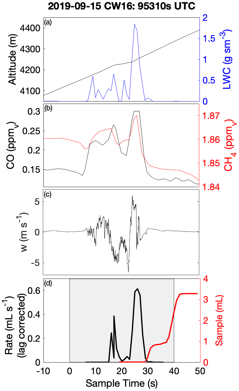
Figure 1Example CW sample merge with auxiliary data for a convective cloud penetration. Time series of (a) altitude and merged LWC, (b) CO and CH4 gas tracers, (c) vertical velocity, and (d) AC3 diagnostic accumulated sample water (right) and estimated lag-corrected collection rate (left). The shaded region indicates the sampling duration, when the AC3 shutter was open, noting that the physical collection of CW within the system can continue for a short duration thereafter.
2.8 Compositional groups
Sea salt (SS) mass was calculated as the sum of the mass concentration of Na+, Cl−, Mg2+ plus fractional contributions of K+, Ca2+ and SO derived from the seawater mass ratio of each species to Na+ (0.037, 0.04 and 0.25, assigned respectively) unless such a contribution exceeded the total measured, in which case the total was used. This approach is grounded in the assumption that Na+ is an exclusive tracer for SS. Non-sea salt (nss) contributions were then assigned to the remaining mass of K+, Ca2+ and SO (nssK+, nssCa2+, nssSO). These groups are used to describe both PILS and CW data. AMS species/groups are expressed without the charge (e.g., AMS NH4) for readability so as to distinguish from the direct measurement of ions by PILS or CW.
2.9 Air-mass trajectories
Back trajectories were generated using the Hybrid Single Particle Lagrangian Integrated Trajectory model (HYSPLIT; Stein et al., 2015) at 1 min temporal resolution along relevant flight tracks and then averaged across designated air masses. Input meteorological data were from the Global Forecast System reanalysis at a horizontal resolution of 0.25∘ × 0.25∘. Transport analysis of flight data was performed using the method described in Hilario et al. (2021).
3.1 Case I: 19–20 September 2019
During this flight, intensifying tropical storm Tapah was situated approximately 600 km northeast of the northern coast of Luzon (23.02∘ N, 127.18∘ E; IBTrACS). A swath of cloudiness associated with a broad band of warm convection was located north of Luzon along an axis approximately WNW–ESE, aligned with the inflow low-level circulation of Tapah, and served as the regional focus of the flight. A second line of convection extended to the southwest approximately perpendicular to the main line, and through the course of the flight, the satellite presentation of this second line became progressively more disorganized. Evidence of episodic cold pool outflow boundaries, marked by arcs of shallow cumulus, could be observed in visible satellite imagery through the course of the flight. An overlay of the flight track atop a visible satellite image taken at 03:30 UTC on 20 September 2019 from the Advanced Himawari Imager (AHI; Fig. 2a) illustrates the sampling strategy in connection with the main convective line and approximately corresponds to the temporal mid-point of the cloud sampling. The primary convective mass associated with Tapah is just off image to the northeast, and the disorganized, northern extent of the second convective line is seen interacting with the western extent of the main study area.

Figure 2Flight tracks (grey) overlaid on visible satellite imagery from the Advanced Himawari Imager (accessed through the CAMP2Ex Worldview Interface: http://geoworldview.ssec.wisc.edu, last access: 9 February 2021) taken near the time of cloud sampling for (a) Case I: 19–20 September 2019, (b) Case II: 23–24 September 2019 and (c) Case III: 15–16 September 2019. Green highlights correspond to periods of extended low-altitude sampling that were used for characterization of the sub-cloud layer structure, trace gases, and aerosols. Red highlights correspond to the cloud modules: in panels (a) and (b) these were “wall” patterns with extended level legs at multiple altitudes within, and near to, cloud. In panel (c) this was a spiral descent with multiple penetrations of cloud at different altitudes. Nearby spiral profiles are highlighted in blue. Cloud water (CW) samples are indicated by cyan-filled circles and in panel (c) an auxiliary CW sample in yellow. Low-level (green, red) and near-cloud-top (cyan) wind vectors are shown using 60 s and leg-mean horizontal wind data, respectively. Designated air-mass locations are shown (see text for details).
The section of the flight track highlighted in red indicates the cloud module (CM) which encompassed a cloud “wall” pattern comprising multiple, sequentially descending, level legs at selected cloud altitudes along the NW–SE axis of the convective line, immediately followed by sampling below the cloud. The sub-cloud legs were arranged approximately perpendicularly (SW–NE) to the cloud legs to assess any cross-track gradients and to increase time outside precipitation for aerosol sampling. The locations of CW collected within the CM are indicated by the cyan circles, illustrating the proximity and high density of the samples. Approximately 150 km to the southeast, low-altitude (< 2 km) sampling was performed earlier on the flight (highlighted in green) in an environment that contained both fair weather cumulus and more vertically developed shallow convection but did not have the same areal extent of stratiform/detrained cloud cover from 1.5 to 3 km that characterized the environment of the CM. The sub-cloud sampling conducted during this period (the downwind survey) provided a direct comparison to the perpendicular transect on the upwind flank of the CM. Spiral profiles extending above the cloud top (highlighted in blue) were conducted at the beginning and end of the downwind survey and upon the completion of the CM. Horizontal wind vectors (20 s mean) are shown (Fig. 2a) on the crosswind sub-cloud legs for both downwind (green) and upwind (red), noting that a marked increase in wind speed was observed in the downwind region, presumed to be attributed to the greater influence of Tapah. A cloud top wind vector (cyan) was calculated using the average of the first (highest) CM leg.

In the vicinity of the CM, the lifting condensation level (LCL) – used to estimate the location of the lowest cloud bases – was estimated at 680 m, and a representative cloud top height was 3.5 km (Table 1). Given that the scene was evolving, the cloud top height estimate is merely a snapshot broadly capturing conditions at the time of the CM; there were nearby cells beyond the sampling area with tops extending above 4 km. Most of the local cloud top maxima appeared (visually) as undulations in the extensive stratiform cloud, which was sampled during two of the CM legs and resulted in the majority of the CW samples. At lower altitudes, cloud coverage was more broken and clustered around cumulus feeding the upper stratiform layers. Precipitation was widespread and was encountered within active cells, between clouds and below the cloud base with a peak rain rate of 5.8 mm h−1 and a mean cloud base rain rate of 4.0 mm h−1.
3.2 Case II: 23–24 September 2019
The same color scheme and features (as described above) were used to annotate the flight track overlaid on an equivalent satellite image (04:00 UTC 24 September 2019; see Fig. 2b). The primary cloud system studied during this case was smaller in spatial extent than Case I but similarly organized as a linear feature with an axis close to that of the low-level wind (NE). In contrast to Case I, vertical shear of the horizontal wind was observed as a directional shift in cloud top winds to northwesterly (above approximately 3 km). The study feature was rooted within a broader area of enhanced shallow convection, while surrounding regions mainly comprised patches of cloud-free and fair-weather cumulus fields. There was no observed maritime deep convection within approximately 500 km.
As per Case I, this flight involved a “wall” pattern CM; however, cloud tops were somewhat higher (∼ 4 km), and more vertical levels were sampled (seven). Upon completion, there was an extended survey within the mixed layer offset from the CM to coordinate sampling with the nearby ship, the R/V Sally Ride, and this pattern provided ample time to fully characterize nearby regions and assess mixed layer spatial variability. A spiral profile followed in largely cloud-free conditions (scattered shallow cumulus) to complement the data collected in clear adjacent regions during the CM (this was more widespread compared to Case I, because of the compactness of the cloudy region). The estimated cloud liquid water path (LWP) was highest in this case, as was the peak LWC (5.6 g m−3) observed near the cloud top.
3.3 Case III: 15–16 September 2019
This flight was dedicated to sampling and characterization of transported biomass burning emissions from Kalimantan fires. A low-altitude survey of the smoke plume was performed approximately perpendicularly to the wind (i.e., from SE to NW) to capture source variability through measurements of trace gas and aerosol abundances. Subsequently, the aircraft repositioned approximately 300 km downwind to probe vertically developed cumulus. Here the CM comprised a spiral descent in proximity to one of these cells, with penetrations through the cloud at seven levels (six of which yielded CW samples), and, near the cloud base, the aircraft then offset to a cloud-free region for a second vertical profile. AHI visible satellite imagery (with flight track overlay and markups per a previous description; Fig. 2c) shows the cloud scene at the time of the descending spiral (04:00 UTC, 16 September 2019). There were far fewer CW samples collected during this case as a result of significantly less time spent in cloud, but each sample corresponded to a single cloud transect. An additional CW sample (yellow marker) was collected near the top of a developing cumulus cloud (4.3 km) shortly after completion of the smoke transect and is included for additional context. The cloud system studied in Case III was distinct from Cases I and II in that (i) convection was isolated and not organized and (ii) precipitation was negligible in the lower half of the cloud. Despite the cloud top being the highest of the three cases (estimate 4.8 km), the development of precipitation appeared to be inhibited by entrainment, which also curtailed high LWC maxima. Both Case II and Case III had similar environmental RH and convective turbulence (as quantified by extrema in vertical winds), yet the apparent impact of the environment on Case III was more pronounced, likely because of its smaller size and earlier stage of maturation. Case III was associated with a significantly higher aerosol abundance as a result of the smoke, and that was observed to affect the cloud microphysics (highest Nd of the three cases), which may suppress warm rain processes (Feingold et al., 2013; Tao et al., 2012) and also enhance entrainment (e.g., Jiang et al., 2006). Low-level winds, from the smoke survey upwind, indicated confluent southwesterly flow across the Sulu Sea, and winds near the cloud top indicated low shear across the target cloud system (Fig. 2c); however, there were clear indications from satellite imagery and the aircraft forward-facing video camera that other more vertically developed cells existed in the vicinity of the CM, and those were affected by northerly shear.
4.1 Boundary layer aerosol
Sub-cloud sampling during Case I included the downwind survey prior to the CM and the upwind transect that formed the final leg of the CM. The upwind transect afforded a simple divide into respective air masses north (UN) and south (US) of precipitation associated with the main cloud line, while the downwind survey identified northern (DN) and southern (DS) air masses based on distinct changes in properties, yielding four air-mass quadrants (Fig. 2a) relevant to the analysis of the cloud complex. Evaluation of the time series during the downwind survey (Fig. 3) showed that below cloud (< 600 m) there were three periods (highlighted in grey background) where aerosol enhancements were coincident with reductions in CO and CH4. Review of the spatial patterns of these gradients and the associated horizontal wind anomalies (for further details, see Fig. S2) provided support for the marked distinction of quadrants DN (aerosol enhanced) and DS (CO enhanced) bestriding a region of confluent flow. The first two crossings into DN occurred during the spiral descent providing snapshots at two altitudes and exhibited a warmer, drier and well-mixed sub-cloud layer, viewed as a regional background environment compared to the cooler, moister and stratified environment of DS, potentially indicative of influence by recent precipitating convection. The jump in CO and CH4 across the boundary was sharp, while the aerosol gradient was diffuse. Comparisons to concurrent time series of O3 and CO2 (Fig. S2) show that O3 exhibited a similar diffuse gradient, and its abundance correlated positively with aerosol and with O3-poor conditions in DS, while CO2 changed sharply across the boundary, analogous to CO and CH4. Elevated CO2 in DS showed significant fine-scale variability (and the highest peak concentrations observed across the sampling region) indicative of local sources, perhaps attributable to active fumarole emissions from the nearby Babuyan Islands. Mean properties of the air-mass quadrants are summarized in Table 2.
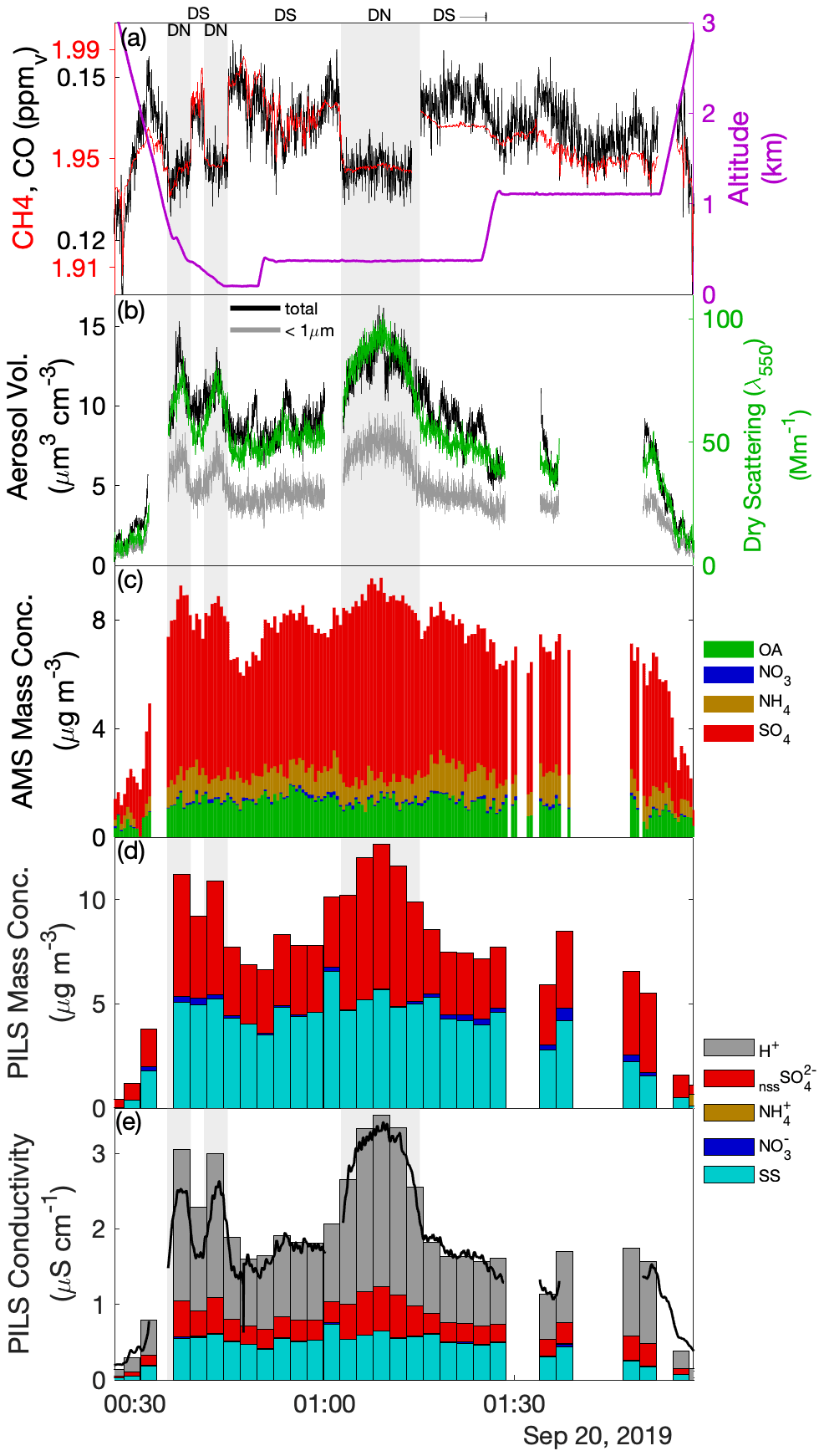
Figure 3Time series of aerosol and trace gases during low-level sampling downwind of the cloud wall during Case I. (a) Gas tracers CO and CH4 and aircraft altitude, (b) bulk aerosol dry scattering at 550 nm and integrated aerosol volume from the LAS for all size and sub-micrometer size bins, (c) AMS-speciated (sub-micrometer) mass concentrations, (d) PILS bulk mass concentrations for major ion groups and (e) PILS bulk conductivity and closure analysis of major ion contributions. H+ ion contributions show the H+ required for charge neutrality. Grey-shaded background regions highlight periods of special interest (see text).
Table 2Case I sub-cloud air-mass properties pertaining to the upwind northern and southern (UN, US) and downwind northern and southern (DN, DS) quadrants surrounding the convective line.
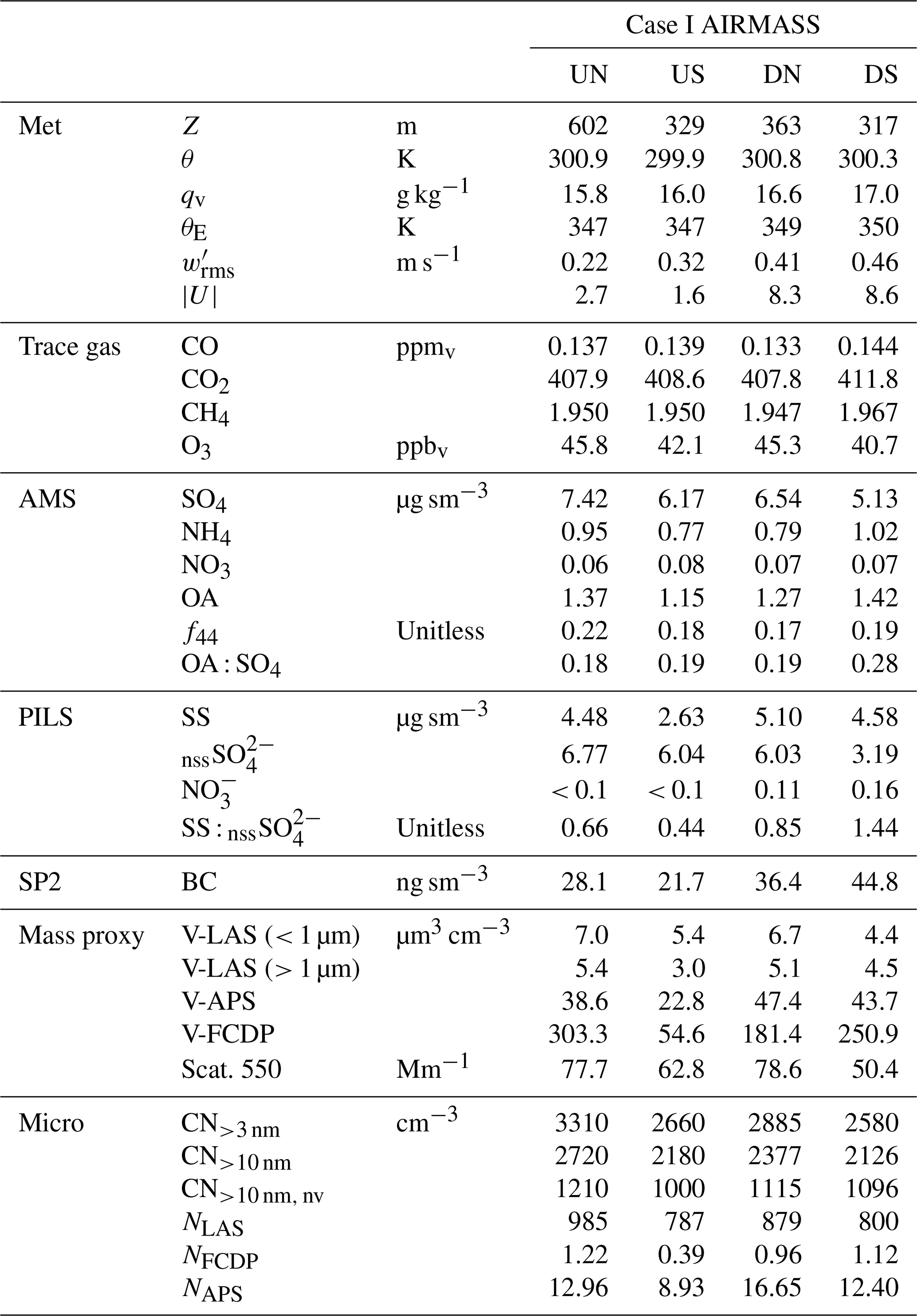
The composition measured by the AMS indicated that the non-refractory aerosol mass was predominantly SO4, with the OA : SO4 ratio varying between 0.18 and 0.28. The highest organic contribution occurred in DS, coincident with the enhanced CO, BC and non-volatile number fraction (i.e., CN CN>10nm), which may indicate that this air mass was more influenced by primary combustion aerosols perhaps originating from transported sources in Luzon or locally from the Babuyan Islands; however, all air-mass quadrants exhibited high f44 (the ratio of 44 to the total OA signal, which is a marker of the organic aerosol degree of oxygenation), and the OA : SO4 was more influenced by changes in SO4 than OA (Fig. 3c). The composition measured by the PILS was strongly dominated by nssSO and SS, with SS : nssSO spanning 0.4–1.4. PILS SS showed a marked reduction in US compared to the relatively consistent concentrations observed in the other air masses, and this reduction was reflected (qualitatively) by proxies for coarse particles (V-LAS>1 µm, V-APS, V-FCDP, NAPS, NFCDP). The aforementioned DN–DS structure seen in dry scattering, V-LAS<1 µm, PILS nssSO and to a lesser degree AMS SO4, was not observed in PILS SS (Fig. 3d), and SS abundances in the downwind air masses may be primarily driven by local regeneration, supported by the higher observed wind speeds. The lower submicron aerosol mass in DS (as quantified by the sum of the AMS constituents) as well as other mass proxies (e.g., scattering and LAS sub-micron volume) supports the prior suggestion of increased precipitation influence on this air mass (i.e., in spite of additional pollution sources), either through direct removal of aerosols or by injection (by evaporatively cooled downdrafts), and subsequent mixing, of overlying aerosol-depleted layers.
AMS NH4 indicated low levels of sulfate neutralization (32 %–34 %) with a minor elevation in DS (53 %), consistent with the insinuation of increased terrestrial influence. Particularly striking was the complete absence of detectible PILS NH in all four air masses, whose only constituents were SS and nssSO, and a very minor contribution from NO (assumed to be associated with the SS given the otherwise acidic conditions). It is unlikely that NH was actually present in the samples but not measured during the lab analysis, because the routinely interspersed standard solutions showed no anomalies in quantification of NH. Further, the independent PILS conductivity measurement shows strong closure with the SS and nssSO under the assumption of balance by H+ (Fig. 3e) for the downwind survey – this is notable because of the strong charge-equivalent conductivity of H+ (approximately 5 times higher than NH), such that closure would not be achieved with other cations. Although NH fractional losses due to volatilization have been documented for the PILS (Sorooshian et al., 2006), this would not explain complete loss, especially under acidic initial conditions. Barring any further explanation for the PILS, it is possible that sulfuric acid particles in the humid tropical boundary layer retain sufficient water in the AMS to challenge the standard fragmentation assumptions (Allan et al., 2004) producing a positive AMS NH4 artifact, due to water interference. The ratio of AMS SO4 to PILS nssSO was found to be 1.02–1.08 for air masses except DS, consistent with a high AMS SO4 collection efficiency (CE) (Zorn et al., 2008). Curiously, the ratio was 1.6 for the DS air mass (which also had higher AMS NH4), but the fractional change in the PILS mass compared to mass proxies (e.g., scattering and V-LAS<1 µm) between DN and DS showed closer alignment (Fig. 3). In this environment, where processing of particles by clouds is almost guaranteed, some degree of internal mixing between SS and nssSO may be expected. In a thermodynamic modeling study, Fridlind and Jacobson (2000) showed that such a mixing state may exert influence over the NH3(g)–NH partitioning in remote marine environments. This does not explain the AMS–PILS discrepancy; however, it highlights a need for further laboratory investigation to determine instrument performance for acidic sulfate under high SS loading, since this pertains to a large range of marine conditions, both background and polluted.
Table 3Case II air-mass properties pertaining to the sub-cloud background (BKGD), characteristic lower free troposphere (LFT) and a perturbed sub-cloud air mass located on the southern flank of the convection (SOUTH). χ and ε0.4 represent mixing fractions and anomalies of the perturbed air mass, respectively (see text).
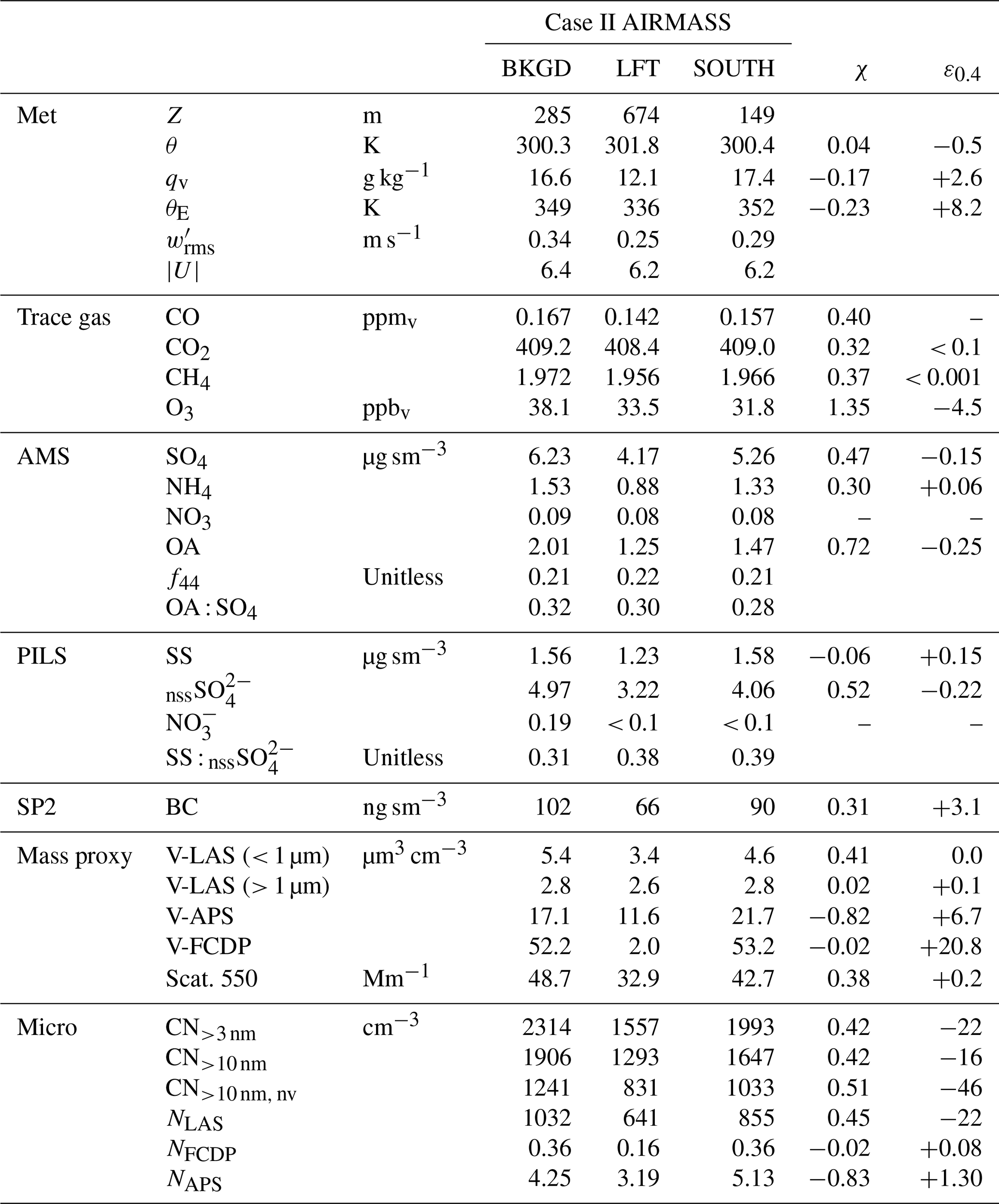
During Case II, low-level sampling occurred upon completion of the CM extending initially to the south of the main line of convection followed by a transect under the convective line and a general survey pattern to the north and west (spanning approximately 180 km), in the vicinity of the R/V Sally Ride. Time series (equivalent to Fig. 3) are shown in Fig. 4 for this period. Aerosol and trace gas concentrations were very steady, with the exception of the two periods highlighted in grey, the latter of which corresponded to the time spent sampling to the south of the cloud line (see Fig. 2b, SOUTH), while the former period was encountered immediately after exiting a region of precipitation near the cloud base at the upwind (i.e., northeastern) end of the cloud line. Even through no altitude change occurred, a rapid increase in potential temperature (θ) was observed (∼ 1 K) as shallow cumulus on the periphery of the main convective line quickly dispersed. This layer was thermodynamically just above the (locally cloud-free) boundary layer in the lower free troposphere (LFT) and was accompanied by a marked reduction in water vapor (qv), CO, CH4 and aerosols. Similar vertical structure and properties were observed during the spiral climb at the end of the low-level survey (approximately 2 h later and 200 km to the west), and we interpret LFT as a representative reference state of the broader LFT, although it cannot be definitively stated whether the sharpness of the gradients atop the mixed layer were reflective of the larger-scale background (and upwind) conditions or a dynamic response to the nearby convection. All other periods of the low-level survey (BKGD) were conducted within the boundary layer and occurred mainly north and west of the convective line in a region that was characterized by a mixture of cloud-free regions and shallow, non-precipitating cumulus clouds and, based on Fig. 4, was free of underlying larger-scale gradients that may confound any interpretation of cloud/precipitation effects on aerosols – we consider this air mass the unperturbed background. A summary of the air-mass properties for BKGD, LFT and SOUTH can be found in Table 3.
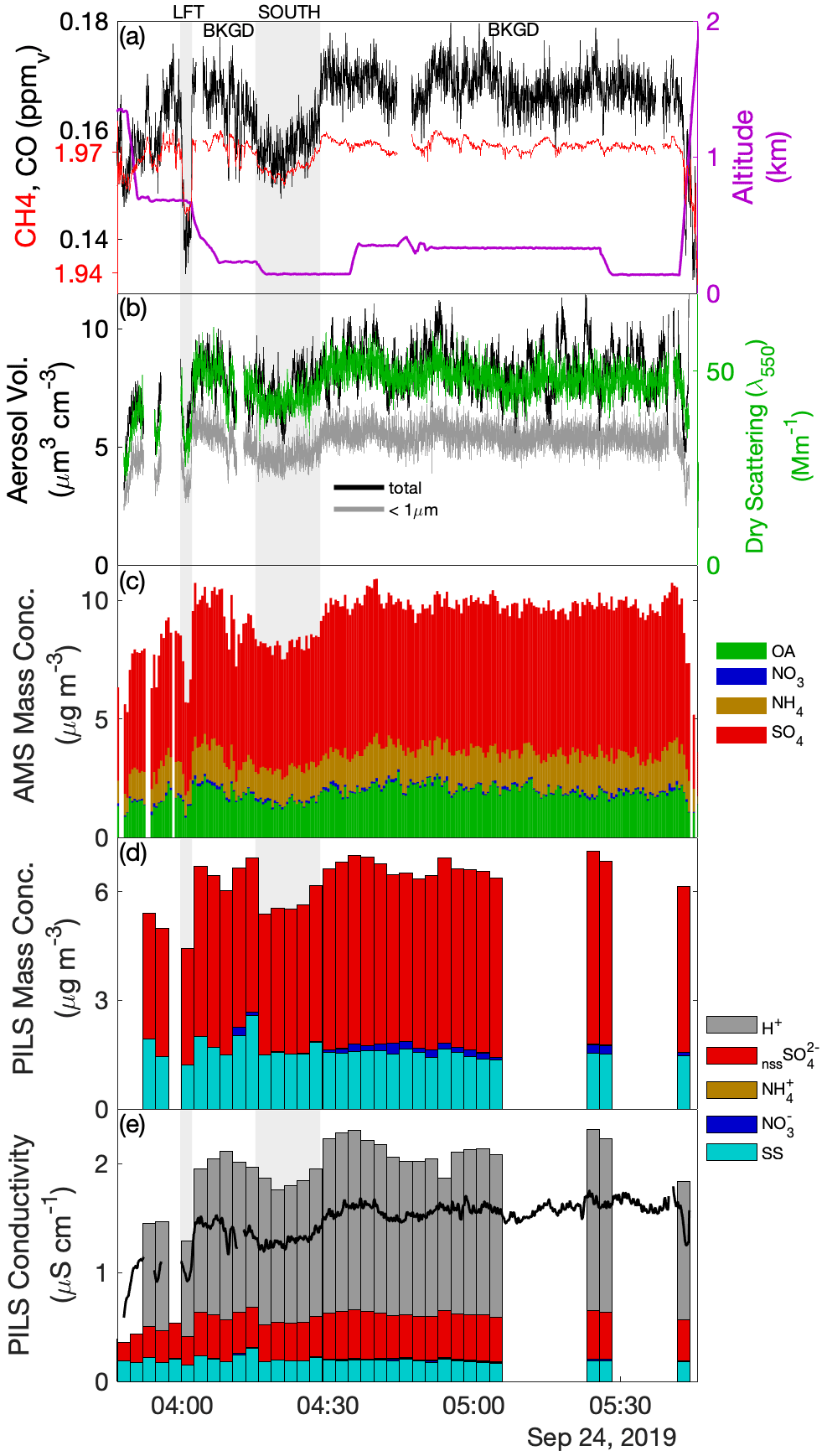
SOUTH represents a perturbation of the near-surface environment compared to BKGD, with approximately 15 %–20 % reduction in aerosol (as quantified by scattering, V-LAS<1 µm and AMS SO4 measurements). The extent to which the properties of SOUTH could be explained by entrainment and subsequent mixing of LFT into BKGD was evaluated by calculating a putative linear mixing fraction, χ, for each property (Table 3). Zero values of χ result from no perturbation from BKGD, values of unity imply equality with LFT, while values outside the unit range necessitate processes other than mixing. Long-lived, passive trace gases (CO and CH4) imply χ ≈ 0.4 and were regarded as the most suitable given that net local sources were unlikely. CO2 also showed broad agreement (χ = 0.32), but the dynamic range was small. A large number of observations that characterize the properties of sub-micrometer aerosol (AMS SO4, PILS nssSO, V-LAS<1 µm, dry scattering, all CN, NLAS) indicated mixing fractions in the range 0.38–0.52, suggesting that the downward mixing implied by the trace gases could also explain the reduction in these aerosol properties. A second metric was computed, ε0.4, defined as the observed anomaly in SOUTH relative to that expected for χ = 0.4 (based on the mixing fraction of CO). Based on positive anomalies, PILS SS and corresponding coarse-mode proxies (V-LAS>1 µm, V-APS, V-FCDP, NFCDP, NAPS) all indicated a net coarse particle source in SOUTH, with many unexplainable by mixing in any proportion, while O3 and OA (marginal) indicated a net sink. The degree of mixing and the location of SOUTH on the down-shear flank of the line of convection suggest that evaporative cooling of precipitation falling through the dry LFT air mass could have been the driver of its downward transport. The thermodynamic variables (θ, qv, θE) indicate moistening and cooling, but a net source of θE (conserved under evaporation of hydrometeors) likely implies an additional contribution from surface fluxes. SOUTH cannot be considered a “cold pool” since it is not cold; however, it displays the hallmarks of an air mass that has been affected by penetrative downdraft-induced mixing (in the recent past), followed by a surface flux-driven recovery perhaps accelerated by surface gustiness. The collective net effect is a higher surface layer θE, coarse aerosol enhancement from sea spray fluxes and surface O3 uptake but, crucially, only marginal net losses observed in the sub-micrometer aerosol budget.
Aerosol composition was similar to Case I: specifically, the PILS composition was dominated by SS and nssSO (with a lower SS : nssSO of 0.31–0.39) and AMS SO4 was the dominant species, with the slightly higher OA : SO4 (ranging from 0.28 to 0.32) with a similar OA age marker (f44 = 0.21). Comparable to Case I, the PILS samples were absent of NH, while the AMS NH4 indicated 56 %–67 % sulfate neutralization (i.e., indicative of ammonium bisulfate). Ratios between AMS SO4 and PILS nssSO were 1.25–1.30, suggesting high CE but also leaving open the possibility of contributions to AMS SO4 from non-refractory species not detectible by PILS as nssSO, such as organosulfates (Farmer et al., 2010; Surratt et al., 2007). Although the PILS composition was similar to Case I, the conductivity closure afforded by Case II (Fig. 4e) was not as complete, with the estimated H+ required for charge balance exceeding the total ion conductivity by 48 %. For reference, replacing the H+ with the equivalent molar concentration of NH to neutralize the sulfate would underestimate the total ion conductivity by 26 %; alternatively, a 65 % NH/35 % H+ mixture would achieve optimal closure (assuming no other contributing constituents). This level of neutralization supports the AMS data suggesting bisulfate but, if correct, does not provide an explanation for underprediction by offline IC.
Case III provided an opportunity to investigate both (i) the variability in aerosol composition attributable to source heterogeneity for a major biomass burning transport event over the Sulu Sea and (ii) the downwind evolution. A time series of a crosswind transect across the biomass burning plume (Fig. 5) illustrates the structure of the plume and shows concentrations that were highly variable in both the vertical and horizontal. A series of short, stacked legs were flown close to the end points of the transect, with substantial aerosol enhancements (dry scattering > 200 Mm−1) extending up to around 2.5 km. The vertical structure of the plume was not consistent between the two sets of stacked legs, nor was there a monotonic decrease in aerosol abundance with height. Analysis of the upwind air-mass history (not shown) provides strong support that fires in southern Kalimantan are the source of the smoke with an age of between 48 and 72 h. Despite the potential for source variability across the transect, differences in secondary aerosol production and variable influence of prior cloud processing, there is a close correspondence in the plume structure amongst CO, dry scattering, LAS volume and OA, which is the largest component of the submicron aerosol mass.
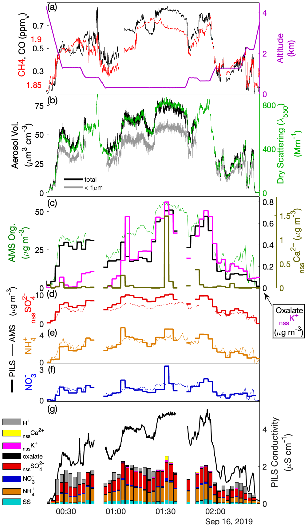
Figure 5Like Fig. 3 but for the upwind cross-plume transect (TX) during Case III. Here, panels (a), (b) and (g) follow panels (a), (b) and (e) from Fig. 3, but panels (c) and (d) have been replaced with (c) comparison of AMS organic mass concentration with PILS biomass burning ion tracer (d–f) comparison of PILS and AMS nssSO, NH and NO, respectively. The contributing species for the conductivity closure has been augmented.
Oxalate, nssK+ and nssCa2+ were found to be enhanced in the plume (Fig. 5c), consistent with other studies of biomass burning (Andreae, 1983; Yamasoe et al., 2000; Maudlin et al., 2015). Oxalate initially tracked OA during the southeastern set of stacked legs (00:30–01:00 UTC) comprising approximately 1.5 % of the OA mass and then remained fairly constant despite an increase in OA through the central section of the transect (dropping to ∼ 0.7 % of OA) before rebounding near the northwestern section (∼ 01:30 UTC). During the subsequent stacked elevated legs oxalate broadly tracked OA, except during the latter half of the highest leg where it remained constant despite rising OA. nssK+ was generally lower at the southeastern end of the transect relative to OA, potentially as a result of fuel differences or mechanisms that resulted in higher loss of primary aerosol in that section of the plume. nssK+ and (more significantly) nssCa2+ exhibited periodic high anomalies (e.g., 01:06, 01:30 UTC) but exhibited neither correlation with the other data shown in Fig. 5c nor covariability with microphysical coarse-mode proxies (e.g., V-APS, V-FCDP) that could confirm similar fine-scale structure in crustal material. A possible explanation relates to the performance of the PILS when sampling coarse and insoluble (or low-solubility) particles such as ash and/or crustal material associated with biomass burning. In the PILS, droplet growth and separation from the airstream as an aqueous solution are relatively well constrained for soluble material; however, Wonaschütz et al. (2019) describe accumulation of insoluble material on the wicking material and impactor in association with laboratory experiments performed with soot particles, while Orsini et al. (2003) also noted similar limitations for low-solubility calcium salts. We hypothesize that under constant rinsing, and particularly under varying environmental conditions, low-solubility crustal deposits may leach, or become detached, back into the PILS liquid stream in a process that is unlikely to be steady or controlled, perhaps explaining the intermittent structure. Other explanations, such as artifacts introduced during offline analysis, are less likely since these spike enhancements are significantly higher than variability observed in sample blanks and were not observed in other phases of flight outside of the biomass burning plume. While this does not help to reconcile the fine-scale temporal structure of nssCa2+ (as a proxy for crustal material associated with the biomass burning), the quantification was assumed to be suitable for assessing average plume properties, on the basis that spike enhancements did not continue after leaving the plume. Associated with the nssCa2+ spikes were positive anomalies in NO and NH, which otherwise showed very close agreement between AMS NO3 and NH4 (Fig. 5e–f). This pattern may be indicative of uptake of NO and NH on dust particles associated with the smoke, and it provides an explanation for the large departure of NO at 01:30 UTC.
Comparison of nssSO with the AMS SO4 shows strong coherence across the plume, with a ratio of 0.70–0.74 (Fig. 5d). In contrast to Cases I and II, high neutralization was observed by both PILS NH and AMS NH4, suggesting ammonium sulfate with evidence of NO contributions to accumulation-mode particles, supported by AMS NO3. AMS SO4 exceeded the known AMS CE = 0.5 for pure ammonium sulfate particles (Middlebrook et al., 2012), which may be caused by the large OA component. While a CE < 1 likely also applies to the AMS NH4, we expect a NH volatilization loss for PILS for neutralized ammonium sulfate particles (Sorooshian et al., 2006), explaining the closer AMS NH4–PILS NH agreement and larger difference for sulfate (i.e., where only AMS has reduced CE, compared to Cases I and II). In stark contrast to the other cases, the measured ions (and associated H+ estimate) only explain about half of the measured conductivity (Fig. 5g), an expected result given the large number of organic anions (e.g., associated with carboxylic acids) that are not quantified during IC analysis. The structure of the measured conductivity tracks the previously described proxies for the plume (CO, dry scattering, LAS volume, OA) and captures some of the finer-scale features smoothed out by the discrete PILS samples (e.g., 02:10–02:15 UTC). While there is no means to attribute the residual fraction of the conductivity, the fact that it tracks OA may imply that, collectively, carboxylic acids contribute a relatively constant fraction of OA, despite the relative contribution of individual species (as illustrated by oxalate) being somewhat more variable, and concurs with a consistent f44 = 0.14 across the plume.
The CM for Case III was located about 250 km downwind of the transect. While not a true Lagrangian comparison, it does provide a point of comparison within the plume subject to approximately 8 additional hours of downwind transport. In addition, while small shallow cumulus clouds were present along the upwind transect (and satellite imagery confirmed the presence of shallow cumulus interspersed throughout the environs of the plume's transport history over water), the region of the Sulu Sea near and to the north of the transect appeared to be the first contact for the smoke-laden air mass with more vertically developed maritime cumulus convection. Trajectory analysis taken at the CM location confirmed that the upwind transect (TX) represented an upwind condition; however, the observed confluence of the wind streamlines (Fig. 2c) made further dissection of the region of the plume somewhat uncertain. Trajectory sensitivity in the vertical, temporal and horizontal (see Fig. S3a for details) confirms this, and we demark subsections of the plume transect originating from the likely southeastern (TX-SE) and northwestern (TX-NW) bounds (which happen to capture, in part, the heterogeneity of TX) to evaluate sensitivity to the upwind origin. In lieu of additional information about the temporal steadiness of the advected air-mass properties, these bounds could also capture uncertainty with the temporal mismatch. Ratios of gas tracers (CO, CO2, CH4) provide some additional guidance (see Fig. S3b, c) and likely indicate that the CM is not fed exclusively with TX-SE. TX-NW alone cannot be rejected, but the most plausible explanation given the expected transport is that the plume becomes more homogenized by the CM and TX mean conditions being probably representative. Trajectories across a longer 5 d timeframe (Fig. S4) further highlight the bifurcation caused by the flow pattern around Borneo, which is a likely driver of the varying plume properties across TX. In contrast, Case I and II air-mass distinctions appear more locally driven than influenced by disparate origins at the larger scale.
Table 4Sub-cloud trace gas and aerosol properties for Case III at the downwind location of the cloud module (CM) and the upwind transect (TX). TX was further divided into southeastern (TX-SE) and northwestern (TX-NW) segments. Δ is the dilution-adjusted percentage change from TX to CM applied to aerosol measurements.
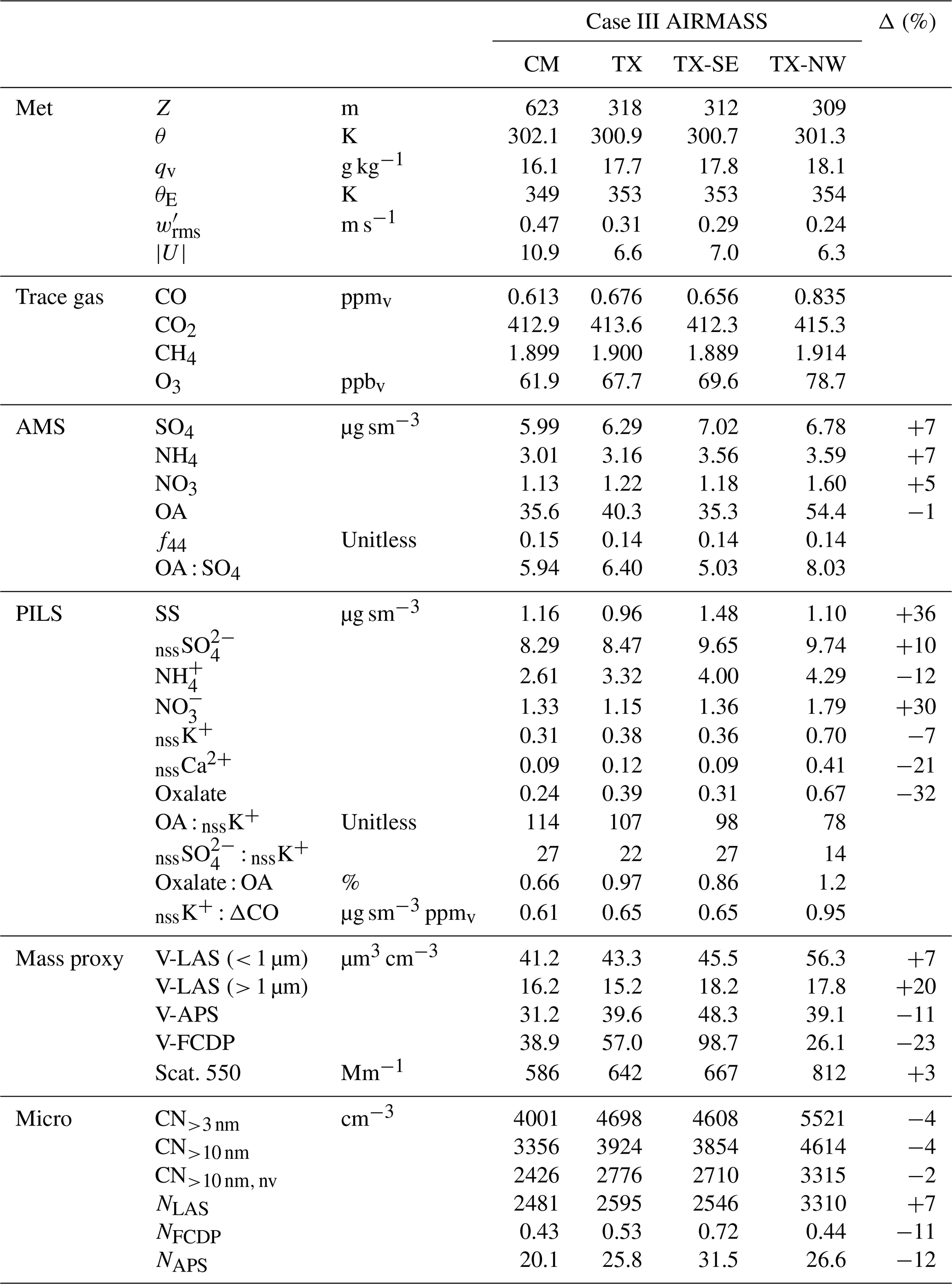
Mean properties of CM, TX, TX-SE and TX-NW can be found in Table 4. The percentage change, Δ, from TX to CM was evaluated by using CO as a dilution tracer, with a 0.1 ppmv background (i.e., for any species X and where ). Given the considerably elevated CO, the result is quite insensitive to the choice of background. The reported evolution is plausible given the expectation of continued plume aging, specifically, a 5 %–10 % increase in AMS SO4, NO3 and NH4 and PILS nssSO in contrast to reductions observed in primary biomass burning aerosol tracers (nssK+ and nssCa2+), and, notably, OA indicates no net change, while oxalate was significantly reduced. Microphysically, a (very) minor decrease in CN is observed along with an increase in accumulation-mode number (NLAS), consistent with coagulation and the further addition of secondary aerosol. Coarse aerosol evolution shows the combined effects of depositional losses of primary biomass burning particles in conjunction with significant addition of SS during passage across the Sulu Sea.
4.2 Non-sea salt sulfate cloud–aerosol mass closure
We construct a simple budget relationship for a cloudy parcel as follows:
X corresponds to AEM concentrations (at standard density) of a non-volatile species found in aerosols and cloud, the left-hand side is the total mass in the cloudy parcel, comprising CW and interstitial (int) components, and the right-hand side relates to accumulated sources and sinks along a cloudy trajectory. Subscript “ML” relates to concentrations found in the sub-cloud mixed layer representative of conditions just before entry into cloud, which we take as the mean concentrations found in air masses: Case I: UN; Case II: BKGD; Case III: CM (see Sect. 4.1). δ is a weighted effective dilution parameter that accounts for dilution caused by entrainment adjusted by the concentration of X found in the environment. Subscript “p” is the chemical production, and “l” is removal by precipitation, both through formation of rain and accretion by rain falling through the parcel. The scavenged fraction, Fs, is defined as the fraction of mass found in droplets relative to the total (e.g., van Pinxteren et al., 2016):
We can use Eq. (2) to rewrite Eq. (1) in a normalized form:
where and . An ideal candidate species for budget closure would not have chemical sources (thus eliminating Fp) and would be size-constrained, such that particles are both large enough to assume near-complete nucleation scavenging at incorporation into cloud but small enough to be fully captured by the size limitations of the aircraft inlet and relevant composition instruments. Four physical processes then influence the budget: (i) the dilution from mixing of environmental air, (ii) the complete evaporation of a subset of droplets (e.g., following inhomogeneous environmental mixing) resulting in a reduction in the scavenged fraction, (iii) a recovery in the scavenged fraction during a recirculation event that follows evaporative loss and reestablishes a state of enhanced supersaturation and (iv) loss and redistribution from precipitation.
Unfortunately, no species entirely satisfies these requirements, but nssSO is a useful candidate because it is abundant across the three cases, it has a low volatility in all forms (thereby negating gas-phase contributions), and it is reasonable to assume that the majority of the particle mass is found in the sub-micrometer size range (i.e., making it readily quantifiable by the airborne in situ aerosol measurements). A PILS–CW nssSO comparison provides the most consistency, but the AMS offers the benefit of improved time resolution, which is valuable for evaluating the clear-air vertical profile and for avoidance of cloud/rain contamination. The AMS SO4 was scaled by a case-specific PILS–AMS ratio under the assumption that the ratio remains near constant at all levels. When considering the expected conditions near initial droplet activation at the cloud base, we estimate that the CCN activation diameter is in the range of 90–180 nm (depending on the case), which translates to > 95 % of the sub-micrometer volume size distribution. In convective clouds it is reasonable to assume that the fraction of particle mass scavenged at nucleation is close to unity (e.g., Jenson and Charlson, 1984). We consider a reference parcel to be one which has Fs = 1 and is undiluted (δ = 0), adiabatic, reversible and with no additional sources/sinks (Fp = Fl = 0), such that XCW = XML. This reference parcel will have a LWC equal to the adiabatic LWC and will retain a constant Nd for which we use the 90th percentile as a broad estimate of typical conditions at initial activation, noting that Eq. (3) is equivalent to normalizing by the reference parcel.
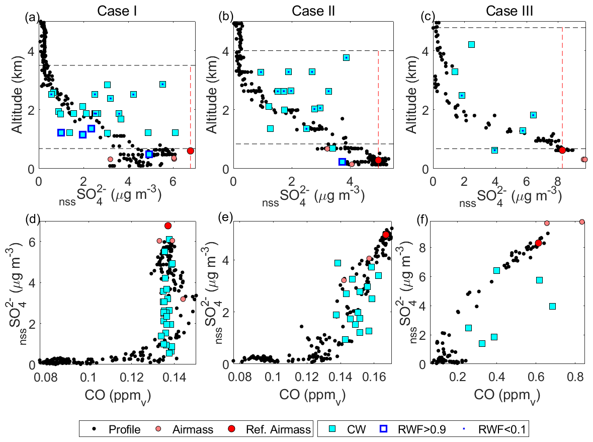
Figure 6(a–c) Profiles showing the relationship between nssSO and altitude for cloudy and clear-air samples in Cases I–III, respectively. Profile data include a combination of spiral profiles in the vicinity of the cloud module as well as sections of the cloud module in clear air. AMS data (included for profiles for improved time response) were scaled for collection efficiency using a case-specific factor (see text). Air-mass data (PILS) are shown, and the reference air mass is highlighted with the vertical dashed line indicating the reference parcel (see text). Cloud water samples (cyan) are also distinguished as non-precipitating (RWF < 0.1) and rainwater (RWF > 0.9). For each case, an estimated cloud top and LCL are marked (dashed black lines). (d–f) Like panels (a)–(c) but showing the relationship between nssSO and CO mixing ratio.
Comparison of CW nssSO with clear column data is made with respect to altitude (Fig. 6a–c) and CO (Fig. 6d–f), as a conserved tracer. In all cases, clear column nssSO shows a general decrease with altitude through the cloud layer. In Cases I and II, the decrease is monotonic, while in Case III, there is a minor enhancement in the upper third of the cloud layer reflecting the ongoing adjustment of the clear column profile to recent (and nearby) convective mixing (i.e., through convective detrainment). Positive curvature in the clear column relationship with CO (Fig. 6d, e) is indicative of net nssSO loss due to precipitation, with more widespread and intense precipitation in Case I resulting in greater curvature. Case III (Fig. 6f), an environment relatively unaffected by precipitation, shows slight negative curvature suggesting net nssSO production (i.e., nssSO concentrations within the cloud layer are higher than mixing alone would indicate).
CW nssSO is generally bounded by the mixed layer nssSO and, with increasing precipitation (i.e., Case I), the variability increases, although there is no dominant altitude trend nor alignment with the clear column profile (Fig. 6a–c). A greater number of CW samples exceed the clear column nssSO at an equivalent altitude consistent with upward transport of sub-cloud air by convection, but conditions where the CW nssSO is lower than the environment are not uncommon (particularly in Case I), suggesting cloudy regions that were either heavily affected by rainout or where mixing with the environment has significantly reduced the scavenged fraction.
Comparison of normalized CW to the microphysical variables (Fig. 7) reveals a pattern where CW nssSO generally exceeds that implied by reductions in condensate from the undilute parcel, implying that rainout alone is not driving the variability amongst samples. The budget of Nd in parcels that have low to moderate RWF normalized by the reference parcel Nd shares many of the same characteristics of Eq. (3), with the major differences being that Fp is absent and there is an additional loss term associated with coalescence scavenging (e.g., Wood, 2006). Complete evaporation of a subset of droplets reduces the scavenged fraction and similarly reduces the droplet number, accretion by raindrops exerts the same first-order influence on both budgets, while partial droplet evaporation occurring during homogeneous mixing does not affect either budget. The comparison between normalized CW nssSO and Nd (Fig. 7b) indicates that when RWF < 0.8, the budget of Nd explains 32 % of the variance in CW nssSO (38 %, 29 % and 64 % if each case is considered separately), and the lack of a slope change from 1 : 1 shown in Fig. 7b suggests that neither coalescence scavenging nor chemical production is a singularly dominant term in the respective budgets. All three cases have undergone aging in the marine atmosphere for timescales that likely exceed the characteristic chemical production timescales for sulfate, especially in cloud. It is reasonable to assume that precursor abundances associated with the major pollutant sources for these air masses have been largely consumed, and resupply of precursors in the marine atmosphere is likely to be low relative to the existing aerosol burden.
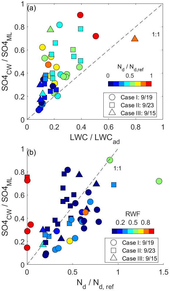
Figure 7(a) Comparison amongst normalized CW nssSO, LWC and Nd. The normalization is with respect to an undiluted parcel originating at the cloud base and a reference droplet number concentration based on the 90th percentile. (b) The same comparison but amongst CW nssSO, Nd and RWF.
Considerable variability exists in attempts to relate normalized CW nssSO to other controlling variables (Fig. 8) with little, if any, statistical correlation. The data are grouped into categories, with three altitude bins representing cloud base, mid-cloud and cloud top, RWF used to separate non-precipitating, rain-in-cloud and rain-only samples, and the mean sample vertical velocity normalized by cloud system turbulence used to identify updrafts, downdrafts and neutral samples. RWF and altitude exhibit co-dependence so emergent patterns may be connected, but the general altitude trend is for a decrease from cloud base to mid-cloud followed by a reversal near the cloud top. A potential explanation is that emergent convective cloud top regions are heavily biased towards energetic parcels that may be less dilute, while mid-cloud regions, although still containing energetic cores, also comprise older, more mixed and, especially in Case I, detrained stratiform cloud. The RWF dependence offers a similar pattern, but a key finding is that for CW nssSO negligible change is found for cloud-free precipitation compared to non-precipitating clouds. CW samples collected in updrafts are, all else being equal, more likely to contain higher CW nssSO, in line with expected convective mass flux of sub-cloud air and the expectation that updrafts would tend to retain a higher scavenged fraction than downdrafts.
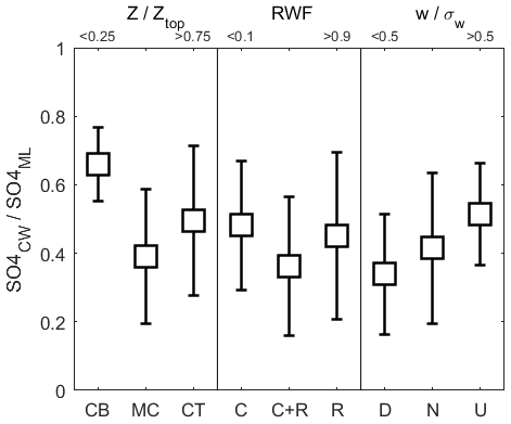
Figure 8Variation (mean ± 1σ) of normalized CW nssSO with altitude, rainwater fraction and vertical velocity (normalized by turbulent rms velocity, σw) incorporating data from all three cases. In each comparison, the data are grouped into categories as follows: altitude: cloud base (CB), mid-cloud (MC), cloud top (CT); RWF: non-precipitating (C), rain-in-cloud (C+R), rain-only (R); vertical velocity: downdrafts (D), neutral (N), updrafts (U).
4.3 Cloud composition
4.3.1 Nitrate and sea salt
Unlike nssSO, where we expect the sub-cloud aerosol measurements (i.e., PILS and AMS) to capture the majority of the total aerosol abundance, total aerosol SS is expected to be underpredicted because of sampling constraints above the inlet 4 µm cut point, making it challenging to directly compare aerosol to the CW SS. CW NO has a multitude of potential sources (e.g., Prabhakar et al., 2014; Leaitch et al., 1986; Hill et al., 2007); however, we can consider three groups: (i) accumulation-mode aerosol activation (e.g., as part of a sulfate–ammonium–nitrate–organic mixture), (ii) coarse-mode aerosol mainly in association with uptake on SS but also potentially from dust, and (iii) gas-phase partitioning of nitric acid within cloud (including reactions that produce nitric acid).
Figure 9a summarizes the relationships amongst NO, nssSO and SS for CW and sub-cloud aerosol from the PILS. PILS SS : nssSO underpredicts the range spanned by CW, and Case III has a lower SS : nssSO in both sub-cloud aerosol and CW – and in alignment with this case is heavily polluted by smoke. The variability seen in CW SS : nssSO can generally be attributed to some combination of the effects of nssSO on in-cloud production, differential scavenging and precipitation loss mechanisms and, potentially, highly localized variability in sea spray. Differential changes in scavenged fraction could manifest as a result of circulations within the convective cloud system that promote regions of sub- and super-saturation along a cloudy parcel trajectory. Similar behavior was demonstrated by Jensen and Nugent (2017), who discussed the condensational growth of large sea salt particles in downdrafts. Notably, this range is substantial for Case I and decreases in parallel with the decrease in precipitation observed between the cases, with Case III exhibiting relatively invariant CW SS : nssSO. CW NO : nssSO is similarly variable, but there is a much stronger relationship between NO and SS on an intra-case basis, increasing in ratio from Case I (0.18) to Case III (0.72). Such a tight relationship between CW NO and SS in Cases I and II is likely indicative that a major fraction of the CW NO is already associated with coarse SS upon activation, while there are indications of additional nitric acid partitioning with altitude (Fig. 9b) in the polluted, largely non-precipitating Case III. Case III also has a CW NO contribution from (previously discussed) accumulation-mode particles (Fig. 5), yielding a higher PILS NO : SS (1.15) than CW (0.72). The opposite is seen in Cases I and II, suggesting that the fraction of SS measured by the PILS (i.e., particle diameter < ∼ 4 µm) contains less NO than the aggregate SS found in CW and may point to an increased degree of internal mixing of SS and nssSO on smaller sea salt particles (e.g., Sievering et al., 1990).
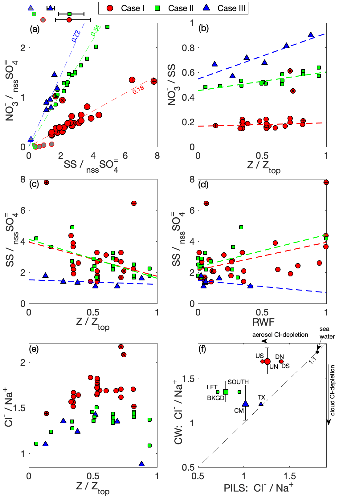
Figure 9Relationships among SS, NO and nssSO. (a) The CW mass ratios of SS to nssSO are compared to mass ratios of NO to nssSO for each case, with relevant sub-cloud air-mass PILS data included for contrast (grey fill). Above the panel, the (geometric) mean SS : nssSO mass ratio is shown (with 1σ variability) for CW for each case. Dashed lines (with slope indicated) show case mean NO : SS mass; (b) CW NO : SS mass against normalized altitude; CW SS : nssSO mass against (c) normalized altitude and (d) RWF; (e) CW Cl− : Na+ mass against normalized altitude; (f) sub-cloud aerosol (PILS) Cl− : Na+ mass ratio compared against the equivalent CW Cl− : Na+ mass ratio. Case I with outlying ratios is highlighted: high-NO pair (×), high-SS pair (+).
The trend in CW SS : nssSO is downward with (normalized) altitude (Fig. 9c) and upward with RWF (Fig. 9d) for Cases I and II. While acknowledging relatively modest correlation, Case I rainwater (RWF > 0.9) exhibits higher CW SS : nssSO (4.24) than non-precipitating (RWF < 0.1) regions of the cloud system (2.39, i.e., an increase of 78 %) and may be indicative of a “giant CCN effect” (e.g., Feingold et al., 1999) where large SS particles are responsible for larger cloud droplets, thereby increasing the likelihood of both acting as precipitation embryos or being collected by existing rainwater. Additionally, large SS is more susceptible to washout than accumulation-mode nssSO, so progressive enrichment of SS in rainwater below the cloud base may be a contributing factor.
Numerous CW samples (20) were collected during two mid-cloud legs of the CM in Case I (Fig. 10) under near-continuous sampling conditions. Four convective periods (marked in Fig. 10a) were identified from enhancements in the w variability that coincided with local LWC maxima, with other periods representing the more quiescent stratiform and non-cloudy but precipitating regions. CW SS and nssSO are locally enhanced in convective periods 1, 3 and 4, coinciding with instances where local enhancement in Nd was observed, indicating fresh lofting of sub-cloud air. The lower leg shows a higher CW SS : nssSO overall and is more dominated by high RWF conditions, and there is a consistent trend in both legs for a downwind decrease in CW SS : nssSO, in line with claimed enhanced removal of SS (but still does not explicitly rule out contribution from in-cloud nssSO production). The recovery from any preferential SS removal appears to be rapid in this sub-cloud environment based on the reported characteristics of air-mass DS, a region observed to be no longer experiencing, but recently affected by, widespread precipitation but through the action of locally increased wind speed having the highest PILS SS : nssSO of the four quadrants (Table 2).

Figure 10Time series of two mid-cloud levels flown during Case I, containing a high density of cloud water samples (20). The key at the top indicates when the aircraft was at the upwind (U) and downwind (D) extents of the cloud module and when on level legs (bold) – note that, unconventionally, descents between levels were not coordinated with the U and D turns. Panels show (a) CW nssSO and SS mass concentration; (b) CW SS : nssSO and Cl− : Na+ mass ratios; (c) LWC and Nd; (d) P and RWF; (e) vertical velocity (w) and aircraft altitude (Z); (f) gas tracers (CO, CO2, CH4 and O3). Also shown are four transects through convectively enhanced regions (dotted line in panels a and b) and the linear trends in the ratios during the level leg sections (b).
SS particles subjected to condensation, or aqueous production, of nitrate, sulfate and organic acids (e.g., Alexander et al., 2005; Chameides and Stelson, 1992; Sievering et al., 1992) tend to liberate Cl− in the form of gaseous HCl (Seinfeld and Pandis, 2016), resulting in a Cl− : Na+ mass ratio that is typically lower than seawater (1.8). Analysis of the aerosol and CW ratios (Fig. 9f) shows evidence of Cl− depletion, with a stronger effect occurring for the aerosol in each case. CW Cl− depletion increases in line with more CW NO, while the aerosol–cloud difference may be explained by the PILS bias towards small SS particles, which aligns with the observed size dependence of Cl− depletion elsewhere (Yao et al., 2003; Keene and Savoie, 1998) and the potential for repartitioning of HCl in the more dilute CW. Excess aerosol Cl depletion (i.e., departure from 1 : 1) is high for Cases I and II (acidic sulfate), where nssSO likely condensed/coagulated or formed on small SS, and low for Case III (neutralized), where small SS particles remain (relatively) externally mixed from the smoke particles. The level of disequilibrium may be greater in Case III, where SS is a recent addition to the aerosol loading. We can observe a decrease in PILS Cl− : Na+ from TX to CM, in line with aging and equilibration of the SS to the abundant acidic gases expected in the smoke, despite some increase in the overall SS (Table 4), while the removal by precipitation in Case I followed by rapid regeneration in the downwind air masses (e.g., DS) indicates an increase in PILS Cl− : Na+ expected with fresh SS. In summary, Case III may be expected to shift further left in Fig. 9f with time, while Case I DS and DN may tend to move slightly left, relaxing towards their upwind counterparts.
A common pattern with altitude is observed (Fig. 9e) with CW Cl− : Na+ increasing in the lower 50 %–70 % of the cloud and then reverting downwards through the upper 30 %–50 %, and the two Case I high-NO outliers correspond to the highest Cl− : Na+, while the two Case I high-SS outliers correspond to the lowest Cl− : Na+ of that case. Reasons behind the shape of the profile are not entirely conclusive, but the consistency between cases is certainly notable. Regions of the cloud systems with the highest Cl− : Na+ align with regions where the aggregate cloud contact time might be longest, suggesting either a relaxation time associated with HCl repartitioning (Keene et al., 1986) as an important contributor or a timescale associated with homogenization of droplet chemistry due to collision/coalescence; however, this falls short when considering the tight grouping of Cl− : Na+ at each vertical level – much tighter than the expected spectrum of cloud parcel ages – while microphysical explanations ought to be less influential on Case III. Differences in temperature sensitivity to gas–CW partitioning amongst the spectrum of contributing semi-volatiles may be a potential factor. For Case I, the altitude dependence can be seen (Fig. 10b) across the two high-density sampling legs, where higher (lower) Cl− : Na+ coincides with the lower (higher) SS : nssSO in the upper (lower) leg and the downwind gradient of decreasing SS : nssSO is accompanied by an increase in Cl− : Na+. Up to this point, in-cloud nssSO production has not been ruled out as a potential driver of the change in ratio; however, all else being equal, this would be expected to drive more Cl− depletion, not less. Instead, precipitation favors enhanced removal of SS (i.e., with lower Cl− : Na+, driven lower by washout of aerosol SS), and the air masses left behind are proportionally enriched in HCl. This is further reinforced by considering the outlier pairs: when removal of low-volatility material is significant (high-NO pair), the Cl− : Na+ is enhanced (in this case even higher than the seawater ratio), while in cases influenced by anomalous additional sea salt aerosol (high-SS pair), the Cl− : Na+ more closely resembles the PILS Cl− : Na+. In the convective periods, Cl− : Na+ was minimally affected (Fig. 10b).
4.3.2 Ammonium
CW NH : nssSO increases from Cases I to III (Fig. 11), a pattern mirrored by the out-of-cloud aerosol data measured by the AMS and (at least for Case III) the PILS. The CW vertical structure is relatively consistent between cases, with a maximum in NH : nssSO between 30 % and 70 % of the normalized altitude very similar to the pattern observed for Cl− : Na+. Profiles of AMS NH4 : SO4 were constructed by averaging AMS NH4 and SO4 over 10 % altitude bins for the lower half and then averaging all data for the upper half – done to mitigate noise in the ratio at low concentration. For Cases I and II, there is no discernable altitude dependence, while Case III shows a reduction only for the upper half bin. Excess aerosol NH in Case III would be expected to demand a significant NH3 vapor pressure that would be available to dissolve in CW. In all three cases, we can assume that almost all NH3 dissolves in CW at equilibrium (Quinn et al., 1987). Despite not measuring NH3(g), we can use this fact to qualitatively explain that, as the aerosol NH : nssSO increases, so too should the positive excess seen in CW NH : nssSO. One result that still lacks explanation is the apparent disconnect of the PILS NH (or lack thereof) observed in Cases I and II.
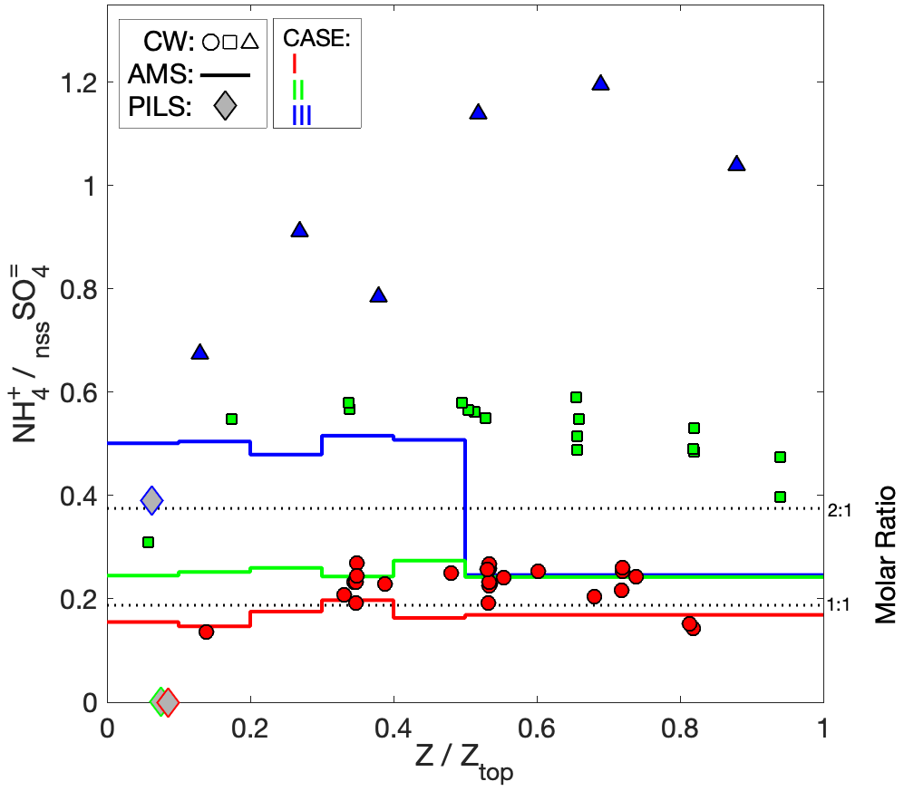
Figure 11Profiles of CW NH : nssSO for each case. Also shown is (i) the mass ratio of mean concentrations of AMS SO4 and AMS NH4 computed in five altitude bins spanning the lower half of the cloud and one bin spanning the upper half of the cloud from adjacent clear-air sampling and (ii) the mass ratio calculated for PILS sub-cloud data.
In Case I, CW NH ranges between 0.14 and 1.3 µg sm−3 (equivalent to 0.17–1.63 ppbv NH3(g)). If this mixing ratio were to exist in the sub-cloud layer in the presence of sulfuric acid particles, then measurable PILS NH would be expected. One possibility is that there is a small background NH3 in the lower troposphere including the cloud layer, but the sub-cloud environment has become extremely ammonia-poor through wet scavenging and surface deposition. This is consistent with oligotrophic surface waters being strongly deficient in NH3 and NH but relies on turbulent entrainment being too slow to replenish the layer. To discount the presence of measurable sub-cloud NH entirely would suggest an overestimate by the AMS, thus requiring an explanation (via, e.g., a water artifact); however, the strong agreement between PILS and microphysical proxies for aerosol mass (e.g., LAS) as well as the internal closure from PILS conductivity make it challenging to discount the data as an instrument failure. In a modeling study, Fridland and Jacobson (2000) found that in remote marine environment conditions with an accumulation mode containing equimolar parts NH4HSO4 and NaCl, the mixing state of particles completely dictated retention (external mixture) or liberation (internal mixture) of NH and Cl−. At the time of writing, some of the authors are in the process of designing a laboratory experiment attempting to recreate conditions pertinent to Cases I and II to investigate the effect of (i) sulfate neutralization, (ii) aerosol water and (iii) mixing state with sea salt on the respective performance of the AMS and PILS.
4.3.3 Cloud pH
Most of the CW samples (47 of 50) were analyzed for pH (Fig. 12) ranging from 3.82 to 5.32 with mean 4.41, and while the differences were quite modest, Case III had a slightly lower mean pH (4.16). All cases showed an increase in pH with altitude, with the largest change occurring for Case I. An increase in pH is expected under increasing LWC and in the presence of enhanced partitioning of basic gases (e.g., NH3). In Case II, the high pH samples observed near the cloud top also contained enhanced nssCa2+, suggesting influence of entrained dust. Overall consistency between cases is notable given the differences in composition and aerosol abundance and, while Case I could be expected to exhibit the most acidic aerosol (under typical boundary layer conditions), Case III had the most acidic clouds. The monotonic profile in pH is also in stark contrast to the more complex pattern seen in NH : SO and Cl− : Na+, indicating that acidity alone was not the controlling factor on the vertical structure of those ratios.
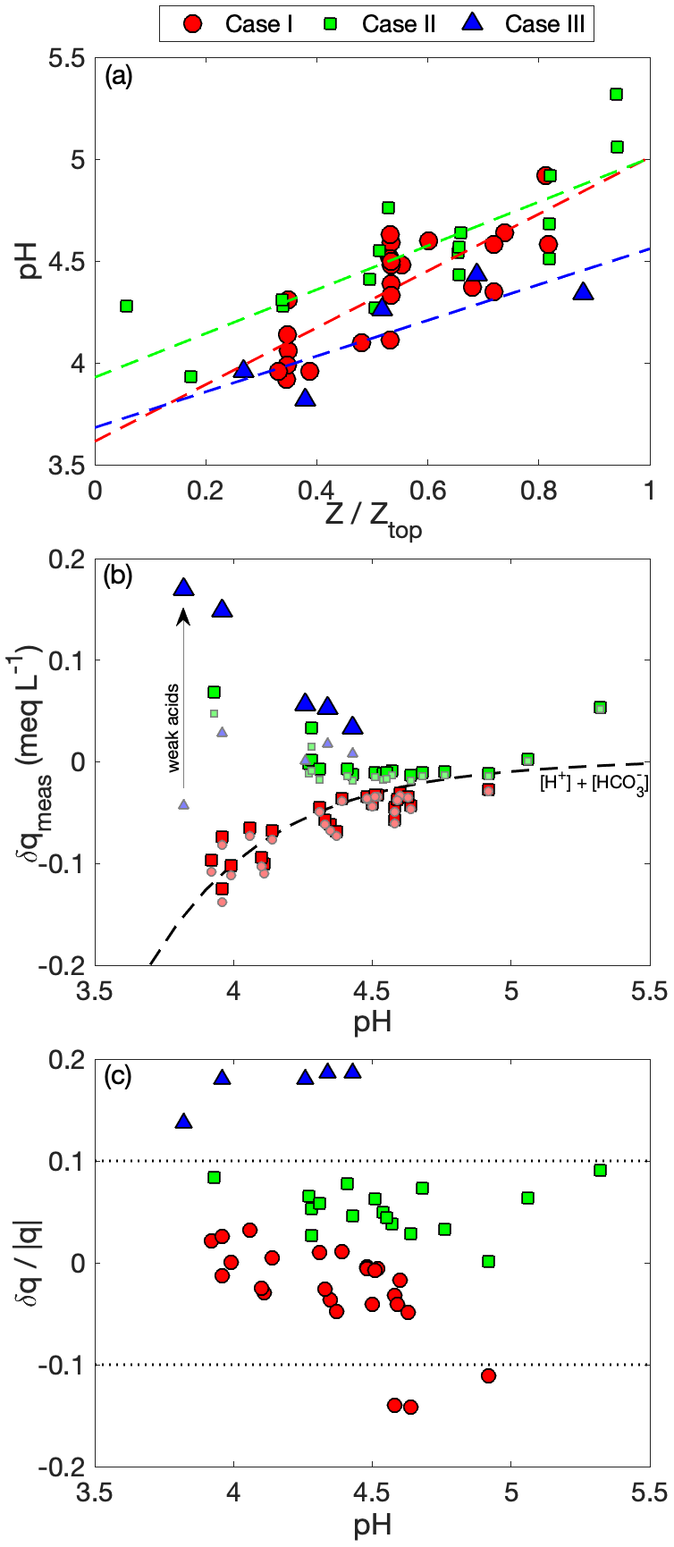
Figure 12(a) Relationship of CW pH with normalized altitude; (b) pH-charge balance closure analysis: residual charges from measured ions are shown including (solid, large) and discounting (desaturated, small) weak acid dissociation, with the black dashed line indicating expected charge imbalance at each pH and (c) residual charge from (b) normalized by the total measured charge. The region bounded by the dotted lines indicates a nominal ±10 % zone that is likely indistinguishable from analytical biases.
Also reported (Fig. 12b, c) is a charge balance assessing the completeness of the measured ion concentrations. Smaller, semi-transparent markers (Fig. 12b) indicate net charge (maximum available) based on the 21 contributing species. The ambient net charge (large, solid markers) was calculated using dissociation equilibria for each species at the measured pH, which should balance the combined charge from H+, HCO (dashed curve) plus anything left unaccounted for. HCO was estimated using a fixed CO2 mixing ratio of 400 ppmv; however, its impact on charge for pH < 5 is negligibly small. Closure for Case I was very good, confirming the simplicity of the composition, while Case II showed an anion deficit at the low and high pH extremes. In Case III, a sizable fraction of the total anion charge was associated with formate, acetate and the second deprotonation of dicarboxylic acids – these weak acids are not effective at lowering the pH to the observed range. Additional unmeasured anions associated with stronger acids (pKa < ∼ 3.5) would be required to achieve closure. Figure 12c shows the residual charge (i.e., the difference from the dashed line, accounting for dissociation) normalized against the total measured (sign-independent) as a measure of relative imbalance. Uncertainties associated with ion chromatography yield some cancellation for charge balance when errors are common to anions and cations; however, calibration uncertainties and blank corrections (blanks are not meaningful for pH measurements due to nonlinearity and buffering) ultimately limit the interpretability of the residual charge. From this, it can be seen that imperfect closure for Case II appears as a small systematic offset likely inseparable from analytical uncertainty, while Case III has a 14 %–19 % residual charge that suggests that unmeasured organic acids make up a relatively constant contribution on a fractional basis.
4.3.4 Organic closure
TOC was measured for a subset of the CW samples (35 of 50) and compared (Fig. 13a) to the 11 speciated organic ions by taking the sum of the organic carbon attributable to each ion (i.e., weighted by species carbon mass fraction), which we describe, for convenience, as organic ion carbon (OIC). The imprint of the biomass burning emissions on the cloud chemistry of Case III is clearly evident through the 5–10-fold increase in both TOC and OIC compared to Cases I and II. A notable result is the consistency of the fraction of TOC explained by OIC, with a regression (total least squares; all cases) indicating that OIC comprises 25.6 % of TOC (R2 = 0.81). Individual OIC : TOC ratios indicate inter-case means that are not statistically different (p > 0.1 for any pair of cases based on a Welch t test), and the finding is similar to Stahl et al. (2021), who conducted a regional survey using the complete CAMP2Ex dataset and found that 70 % of the TOC was unaccounted for by ions. For readability in the plot, the three points associated with Case III have been scaled by a factor of 10.

Figure 13(a) Closure of the sum of the carbon contribution from each measured organic ion – the organic ion carbon (OIC) – against measured total organic carbon (TOC), with Case III scaled by a factor of 10 to aid readability. Inset is a histogram of the OIC : TOC ratio colored by case, and a total-least-squares (TLS) best fit line for the OIC–TOC closure is included. (b) Closure analysis for CW TOC and sub-cloud organic aerosol (OA) from the AMS. The CW data are normalized by CW nssSO, and OA data are scaled by an estimate of carbon mass fraction (fc) and normalized by AMS SO4. “Air-mass” means are included with a 1σ bar aligned with the “air mass” most relevant to the cloud (as per Fig. 9; here, only outlying air masses are labeled to aid readability). As in panel (a), Case III is scaled by a factor of 10. The contributions to TOC arising from measured acetate (A), formate (F) and oxalate (O) are shown next to each case with the same normalization.
Of the 11 speciated organic ions, (i) DMA was not detectable in any of the CW samples (i.e., spanning all cases), (ii) maleate was absent in Cases I and II and only detected in a limited subset of Case III (4 of 6), (iii) in Case III, glycolate was only detectable in one sample (this species elutes near acetate, which was strongly enhanced, masking its detectability), (iv) succinate and adipate co-elute are considered in tandem (as succinate – only Case I contained a few samples (7 of 27) that were analytically judged to be adipate), and (v) MSA was not detectible in half the Case III samples. The major organic ion contributions were from formate, acetate and oxalate, in varying proportion, with succinate more considerable in Case III (Table S3). CW MSA : nssSO was 0.26 % and 0.43 % for Cases I and II, which is close to the lower bound reported by Bates et al. (1992) for submicron particles in biogenically influenced marine air masses. They found that, under warm tropical maritime conditions, biogenic sulfur precursors (e.g., dimethyl sulfide) do not favor the MSA production pathway (thus making it a poor discriminant for evaluating biogenic sulfur contributions in this scenario); hence, on these grounds, we cannot negate a (partial) contribution to nssSO from marine biogenic origin, but we can conclude that there are no significant sources of MSA (including in-cloud production) affecting these two cases. In Case III, for the three samples where MSA was detected, the ratio is even lower (< 0.1 %), strongly indicating that this smoke plume is not enriched in MSA, at least insomuch as it affects clouds, despite the particulate sulfur content (i.e., nssSO) of the plume being quite high.
In spite of its contribution to organic ions in CW, oxalate was not detected on the acidic particles sampled by the PILS in Cases I and II, suggesting that, like NO, oxalate is neither thermodynamically favored on smaller SS particles (that are perhaps enriched in additional nssSO) nor sulfuric acid/ammonium bisulfate particles externally mixed from SS. Size-resolved aerosol sampling within the region has shown oxalate present on both fine and coarse particles (Cruz et al., 2019), and in the absence of a neutralizing base, oxalate may repartition/volatilize to oxalic acid in the gas phase (Paciga et al., 2014), which may inhibit fine-mode oxalate compared to the data of Cruz et al. (2019). In a sub-tropical marine environment, Turekian et al. (2003) found an increase in oxalate relative to MSA (i.e., another secondary aerosol tracer) with size, in support of the inclination of oxalate towards coarse SS, but argued that its formation on SS was related to marine organic precursors. Although no supporting gaseous measurements were available, we make the assumption that acetate and formate reside as gaseous acetic and formic acid when outside cloud. The partitioning of the other measured carboxylic acids is unknown, but their contributions to TOC closure are small.
AMS OA represents a particle-phase contribution to CW TOC, subject to cloud scavenging. An OA carbon mass fraction (fc) calculated from elemental O : C based on AMS f44 (Aiken et al., 2008) scales the OA to allow comparison on a carbon mass basis – assumed to be more constrained than attempting to convert the incomplete CW composition to organic mass. In Cases I and II, the contribution of AMS OA carbon to CW TOC was found to be 48 % and 35 %, respectively (Fig. 13b), and an additional 20 % and 24 % relate to the carbon contribution from acetate, formate and oxalate (assumed not to overlap with AMS OA), leaving a residual 32 % and 40 % from water-soluble organic gases (WSOG) – such as alcohols, aldehydes and additional carboxylic acids – and unmeasured coarse-mode organic contributions. Comparing Cases I and II, the AMS OA : SO4 increases by 78 %, while CW TOC : nssSO increases by 120 %, highlighting a general enhancement in the contribution of organic species to both cloud and aerosol, but the increased TOC fraction of acetate and formate is perhaps indicative of the more general influence of WSOG on CW TOC in Case II.
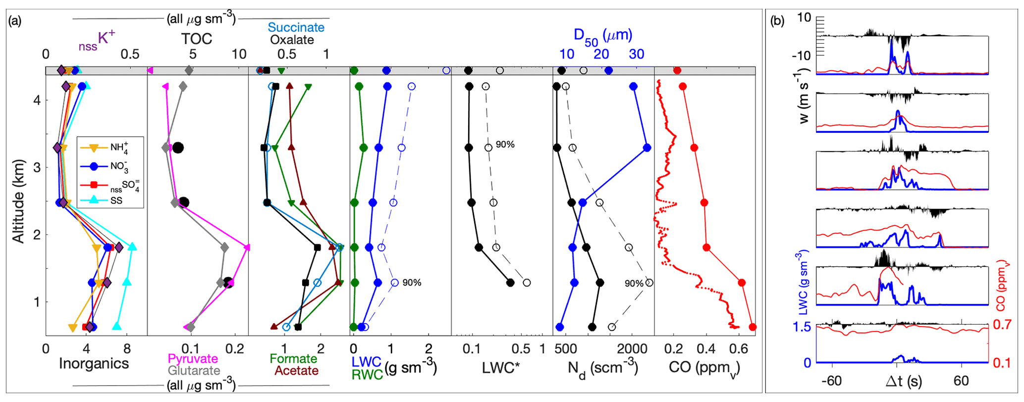
Figure 14(a) Profiles of key CW species during the Case III cloud module and supporting microphysical (LWC, RWC, adiabatic ratio (LWC∗), Nd, volume-based median diameter, D50) and gas tracer (CO) data. Also shown alongside CO is the CO profile in the nearby (cloud-free) environment. Included in the grey-shaded region is the corresponding data from a cloud top penetration near the upwind transect (yellow marker, Fig. 2; see text). (b) Thumbnail time-series plots (±75 s from center lines) of the six cloud penetrations corresponding to the CW samples showing LWC, CO and w, with all plots equally scaled.
In Case III, the availability of AMS OA carbon was found to exceed CW TOC (Fig. 13b). In addition, coarse-mode organics and WSOG cannot be discounted as also contributing to CW TOC, but we might expect more overlap in the measured CW organic ions with AMS OA, since the thermodynamic environment is more conducive to these acids being found (in some proportion) on accumulation-mode particles (e.g., because of higher NH). A specific unknown is any potential difference in CE between AMS OA and AMS SO4, the latter having been reported as 0.7–0.74, based on PILS nssSO, with the former not being verifiable. A second explanation for the apparent exceedance of OA is that the scavenged fraction may be lower for the less hygroscopic organic matter compared to sulfate or that organic-rich droplets may be smaller, causing them to be undersampled in CW (because of decreased collection efficiency at D < 20 µm). With such a high number of potential CCN in Case III (NLAS = 2100), peak supersaturations would be suppressed, leading to an increase in the critical diameter for droplet activation; however, this is offset by the larger size of biomass burning particles (LAS volume mode = 446 nm), so any difference in the propensity for organic- or sulfate-rich particles to activate as CCN is likely to affect only a small proportion of the total mass. Furthermore, the OA is such a large fraction of the sub-micrometer mass (AMS OA : SO4 ≈ 6) that the OA mass distribution should be fairly consistent with the LAS volume distribution, so a strongly size-dependent composition is not able to reconcile the apparent reduction in OA in cloud. A more detailed review of the vertical structure (Fig. 14) suggests that entrainment would tend to drive further increases in the interstitial mass fraction through droplet evaporation, especially in the upper half of the cloud, where the magnitude of the reduction in CW AEM and Nd (∼ 3–5-fold) is far larger than the dilution (as quantified by the reduction in the in-cloud CO above the background). The vertical velocity structure observed in the upper half of the cloud (Fig. 14b) also indicates that active growth of the current cell has likely ceased, with some of the higher LWC regions embedded within downdrafts. This is likely to favor expulsion of CW AEM, thereby enhancing the interstitial fraction, while in weakly recirculating regions reactivation may be even more biased to larger and more hygroscopic particles than during initial activation at the cloud base. In contrast, the transect at ∼ 1.3 km comprised a strong (∼ 7 m s−1) updraft collocated with the peak LWC, CO enhancements commensurate with the sub-cloud layer and high Nd indicative of a fresh convective element. We hypothesize that partial evaporation and recirculation, in response to the pulsed nature of cumulus convection, drive a sorting mechanism that preferentially deactivates droplets containing low-hygroscopicity residuals. Microphysically similar effects, chiefly in relation to droplet spectral broadening, have been explored in relation to droplet size and solute content influences on diffusional growth rates (e.g., Wood et al., 2002) and, specifically, in relation to circulation-induced deactivation and reactivation (Yang et al., 2018). Despite the stark dynamical and microphysical differences, the organic composition was relatively unchanged, at least as inferred from the speciated organic ions. Overall, the structure of the AEM concentrations for the carboxylic acids conforms rather closely to that of the inorganic ions and TOC (where measured), with perhaps a minor relative enhancement in formate and acetate in the upper half of the cloud that could be explained in the same manner as nitrate (Fig. 9) as an increase in partitioning at lower temperatures. There is no indication of an aqueous chemical mechanism dominating the TOC budget, at least at the timescale of this convective cloud system.
We have analyzed the sub-cloud and in-cloud composition for three tropical maritime shallow convection cases. These cases were selected from flights carried out as part of the CAMP2Ex field campaign, specifically because of their high spatial and temporal coincidence between cloudy and clear-air sampling and the availability of a unique CW composition dataset. In each case, sub-cloud aerosol properties and abundances exhibited mesoscale variability that was attributed to a combination of the direct influence of the cloud systems on circulation through convergence of distinct air masses, the impact of vertical mixing and aerosol removal by precipitation and chemical production effects. Although complicating the cloud closure, sub-cloud air-mass variability served as a useful aspect for closure analysis amongst the various aerosol- (microphysical and compositional) and gas-phase instrumentation. The first two cases could be categorized as having aged, polluted/elevated background conditions, meaning that these air masses contained a strong signature of elevated East Asian regional pollution that had resided for several (3–5) days over tropical waters, aging the aerosol properties and largely homogenizing the fingerprint of sources. In contrast, the third case comprised a major smoke transport event from Kalimantan fires. In Cases I and II, the aerosol was dominated by sea salt and nss sulfate with low levels of neutralization suggestive of a mixture of sulfuric acid and ammonium bisulfate, while Case III was fully neutralized by ammonium with nitrate observed on sub-micrometer particles. The ratio of the AMS SO4 to PILS nssSO was near (or greater than) unity for the acidic cases but reduced to 0.70–0.74 for the smoke case, which can be attributed to reduced CE in the AMS. NH was not captured equally between the PILS and AMS for the acidic cases, with the PILS suggesting negligible NH and a relationship with the presence of sea salt believed to be a contributing factor. This ought to be a topic of future investigation under controlled laboratory conditions. The sub-micrometer aerosol in the smoke-enhanced boundary layer of Case III was dominated by organic mass – a factor of ∼ 6 greater than sulfate. In Cases I and II there was evidence that sea salt was quickly replenished following perturbations related directly to precipitation (Case I) and indirectly through downdrafts and surface gustiness (Case II).
The cloud systems studied in the three cases reflected a decreasing significance of precipitation from Case I to Case III and, as such, the clear column relationship between CO and sulfate (used as a ubiquitous aerosol tracer) showed a decreasing curvature. High curvature found in Case I indicated widespread vertical mixing of CO accompanied by net loss of sulfate due to precipitation, while a slight negative curvature found in the largely non-precipitating Case III was indicative of similar vertical redistribution between species along with net sulfate production. There was a high degree of intra-cloud variability in CW solute abundance which can be largely attributed to physical (rather than chemical) mechanisms, affecting the scavenged fraction (e.g., homogeneous and inhomogeneous mixing of cloud-free air) and losses due to rainout. With the exception of a few outlying samples, CW sulfate was generally bound at the upper level by the sulfate concentration in the sub-cloud layer but could also be found to be lower than the clear column abundance at equivalent altitudes. Acknowledging the sources of measurement uncertainty, the current level of quantitative agreement between aerosol and cloud solute abundances (using a sulfate tracer) is certainly encouraging for these complex and dynamic convective cloud systems; however, further improvement in quantification of scavenged fraction and rainout loss likely requires a technique to accurately measure interstitial mass.
Of the other remaining major species contributing to the CW composition, none could yield an effective closure with sub-cloud aerosol because of large contributions from the undersampled coarse-mode particles and gas-phase abundance. In all cases, sea salt was the largest single constituent, by mass, of the average CW composition and implicitly suggested that PILS captured only 10 %–50 % of the total sea salt mass, depending on the case and calculation method. The range of compositional variability between sea salt and sulfate increased from Case III to Case I, in line with an increase in precipitation, and rainwater tended to have higher relative sea salt, which was attributed to (i) a giant CCN effect whereby large sea salt had a greater predisposition to generating large droplets more likely to be involved in warm rain processes and (ii) a greater capture of sea salt by rainwater outside clouds. Nitrate showed a very tight connection with sea salt in all cases, despite being largely absent in the sub-cloud aerosol measured in Cases I and II. These results imply that the nitrate was already associated with coarse sea salt upon incorporation into cloud, and it was only in Case III where a fractional contribution could be diagnosed from accumulation-mode particles (up to 30 %) and additional gas-phase partitioning. Similar findings extended to ammonium and organic species, with CW concentrations exceeding projections from the measured aerosol species, the one exception being the organic closure in Case III. In this instance, 20 %–50 % of the AMS organic aerosol mass was unaccounted for in CW TOC after consideration of carbon fraction, potential CE differences with AMS SO4, and differences in production rates in cloud between sulfate and organics. This may indicate a higher proportion of organic material residing as interstitial relative to sulfate, either through discrimination at activation or through subsequent preferential evaporation as the cloud interacts with dry environmental air. A closure analysis between measured pH and speciated ions indicated that charge neutrality (< 10 %) was achieved in Cases I and II, and an estimated 14 %–19 % additional anion contribution (with pKa < 3.5) was needed in Case III. The carbon from measured CW-speciated organic ions comprised 25 % of TOC, a result that was remarkably consistent between the three cases, despite differences in the relative abundance of the measured organic ions. This result was particularly striking given the order of magnitude difference in concentration between Case III and the other cases but was supported in part by the relatively consistent and high AMS f44 amongst the cases, implying that atmospheric aging, leading to oxidation of organic species, in tropical maritime air masses is quite rapid and consistent, at least in terms of functionality.
| AC3 | Axial cyclone cloud water collector |
| AEM | Air-equivalent mass |
| AHI | Advanced Himawari Imager |
| AMS | Aerosol mass spectrometer |
| APS | Aerodynamic particle sizer |
| BC | Black carbon |
| CAMP2Ex | Clouds, Aerosols and Monsoon Processes – Philippines Experiment |
| CCN | Cloud condensation nucleus |
| CE | Collection efficiency |
| CM | Cloud module |
| CN | Condensation number (used with subscripts indicating the CPC) |
| CPC | Condensation particle counter |
| CVI | Counterflow virtual impactor |
| CW | Cloud water |
| FCDP | Fast cloud droplet probe |
| fc | Carbon mass fraction |
| Fs | Scavenged fraction |
| HVPS | High-volume precipitation spectrometer |
| IC | Ion chromatography |
| LAS | Laser aerosol spectrometer |
| LCL | Lifting condensation level |
| LWC | Liquid water content |
| LWP | Liquid water path |
| ML | Mixed layer |
| Nd | Cloud droplet number concentration |
| nss | Non-sea salt |
| OA | Organic aerosol |
| OIC | Organic ion carbon |
| P | Precipitation rate |
| PILS | Particle-into-liquid sampler |
| qv | Water vapor mixing ratio |
| RH | Relative humidity |
| RWC | Rainwater content |
| RWF | Rainwater fraction |
| SS | Sea salt |
| SP2 | Single particle soot photometer |
| TOC | Total organic carbon |
| w | Vertical velocity |
| WSOG | Water-soluble organic gases |
| 2D-S | Two-dimensional stereo probe |
| χ | Mixing fraction (used for air masses in Case II) |
| θ | Potential temperature |
| θE | Equivalent potential temperature |
All datasets are publicly available and can be found at https://doi.org/10.5067/Suborbital/CAMP2EX2018/DATA001 (NASA/LaRC/SD/ASDC, 2020). Himawari visible imagery was accessed through the CAMP2Ex Worldview Interface: http://geoworldview.ssec.wisc.edu (University of Wisconsin/NASA EOSDIS, 2021).
The supplement related to this article is available online at: https://doi.org/10.5194/acp-22-13269-2022-supplement.
EC, LDZ, MAS, CER, ELW, KLT, JPD, GSD, SW and SCvdH contributed to experimental data collection, and EC, RAB, ABM, CS and AS performed laboratory analysis. All the authors contributed towards manuscript preparation.
The contact author has declared that none of the authors has any competing interests.
Publisher’s note: Copernicus Publications remains neutral with regard to jurisdictional claims in published maps and institutional affiliations.
This article is part of the special issue “Cloud, Aerosol and Monsoon Processes Philippines Experiment (CAMP2Ex) (ACP/AMT inter-journal SI)”. It is not associated with a conference.
We are grateful for the use of imagery from the NASA CAMP2Ex Worldview application (https://worldview.earthdata.nasa.gov, last access: 12 October 2022), part of the NASA Earth Observing System Data and Information System (EOSDIS). We wish to thank the pilots and flight crew of the NASA Wallops Flight Facility P-3 aircraft for their support throughout the CAMP2Ex field campaign. We would also like to recognize the assistance of the NASA Ames Earth Science Project Office (ESPO) and facilities personnel at Clark International Airport in Pampanga, Philippines. Finally, we would like to thank students and staff at the Manila Observatory and Ateneo de Manila University for help in our field laboratory.
This research has been supported by NASA's Radiation Sciences Program, the authors from the University of Arizona were supported by NASA grant 80NSSC18K0148, and Susan C. van den Heever and Gabrielle R. Leung were funded by NASA grant 80NSSC18K0149.
This paper was edited by Lynn M. Russell and reviewed by two anonymous referees.
Aikawa, M. and Hiraki, T.: Washout/rainout contribution in wet deposition estimated by 0.5 mm precipitation sampling/analysis, Atmos. Environ., 43, 4935–4939, 2009.
Aiken, A. C., Decarlo, P. F., Kroll, J. H., Worsnop, D. R., Huffman, J. A., Docherty, K. S., Ulbrich, I. M., Mohr, C., Kimmel, J. R., Sueper, D., Sun, Y., Zhang, Q., Trimborn, A., Northway, M., Ziemann, P. J., Canagaratna, M. R., Onasch, T. B., Alfarra, M. R., Prevot, A. S. H., Dommen, J., Duplissy, J., Metzger, A., Baltensperger, U., and Jimenez, J. L.: O C and OM OC ratios of primary, secondary, and ambient organic aerosols with high resolution time-of-flight aerosol mass spectrometry, Environ. Sci. Technol., 42, 4478–4485, https://doi.org/10.1021/es703009q, 2008.
Alexander, B., Park, R. J., Jacob, D. J., Li, Q. B., Yantosca, R. M., Savarino, J., Lee, C. C. W., and Thiemens, M. H.: Sulfate formation in sea-salt aerosols: Constraints from oxygen isotopes, J. Geophys. Res., 110, D10307, https://doi.org/10.1029/2004JD005659, 2005.
Allan, J. D., Delia, A. E., Coe, H., Bower, K. N., Alfarra, M. R., Jimenez, J. L., Middlebrook, A. M., Drewnick, F., Onasch, T. B., Canagaratna, M. R., Jayne, J. T., and Worsnop, D. R.: A generalised method for the extraction of chemically resolved mass spectra from aerodyne aerosol mass spectrometer data, J. Aerosol Sci., 35, 909–922, https://doi.org/10.1016/j.jaerosci.2004.02.007, 2004.
Andreae, M. O.: Soot carbon and excess fine potassium: Longrange transport of combustion-derived aerosols, Science, 220, 1148–1151, 1983.
Andronache, C.: Estimated variability of below-cloud aerosol removal by rainfall for observed aerosol size distributions, Atmos. Chem. Phys., 3, 131–143, https://doi.org/10.5194/acp-3-131-2003, 2003.
Bae, S. Y., Park, R. J., Yong, P. K., and Woo, J. H.: Effects of below cloud scavenging on the regional aerosol budget in East Asia, Atmos. Environ., 58, 14–22, 2012.
Barrick, J. D. W., Ritter, J. A., Watson, C. E., Wynkoop, M. W., Quinn, J. K., and Norfolk, D. R.: Calibration of NASA turbulent air motion measurement system, NASA Tech. Pap. TP-310, NASA, Washington, D.C., https://ntrs.nasa.gov/api/citations/19970010469/downloads/19970010469.pdf (last access: 12 October 2022), 1996.
Bates, T. S., Calhoun, J. A., and Quinn, P. K.: Variations in the methanesulfonate to sulfate molar ratio in submicrometer marine aerosol particles over the Southern Pacific Ocean, J. Geophys. Res., 97, 9859–9865, 1992.
Bator, A. and Collett, J. L.: Cloud chemistry varies with drop size, J. Geophys. Res.-Atmos., 102, 28071–28078, https://doi.org/10.1029/97jd02306, 1997.
Baumgardner, D., Raga, G. B., Jimenez, J. C., and Bower, K.: Aerosol particles in the Mexican East Pacific Part I: processing and vertical redistribution by clouds, Atmos. Chem. Phys., 5, 3081–3091, https://doi.org/10.5194/acp-5-3081-2005, 2005.
Beard, K. V.: Terminal velocity and shape of cloud and precipitation drops aloft, J. Atmos. Sci., 33, 851–864, 1976.
Bela, M. M., Barth, M. C., Toon, O. B., Fried, A., Homeyer, C. R., Morrison, H., Cummings, K. A., Li, Y., Pickering, K. E., Allen, D. J., Yang, Q., Wennberg, P. O., Crounse, J. D., St. Clair, J. M., Teng, A. P., O'Sullivan, D., Huey, L. G., Chen, D., Liu, X., Blake, D. R., Blake, N. J., Apel, E. C., Hornbrook, R. S., Flocke, F., Campos, T., and Diskin, G.: Wet scavenging of soluble gases in DC3 deep convective storms using WRF-Chem simulations and aircraft observations, J. Geophys. Res.-Atmos., 121, 4233–4257, https://doi.org/10.1002/2015JD024623, 2016.
Benedict, K. B., Lee, T., and Collett Jr., J. L.: Cloud water composition over the Southeastern Pacific Ocean during the VOCALS regional experiment, Atmos. Environ., 46, 104–114, 2012.
Berg, L. K., Shrivastava, M., Easter, R. C., Fast, J. D., Chapman, E. G., Liu, Y., and Ferrare, R. A.: A new WRF-Chem treatment for studying regional-scale impacts of cloud processes on aerosol and trace gases in parameterized cumuli, Geosci. Model Dev., 8, 409–429, https://doi.org/10.5194/gmd-8-409-2015, 2015.
Blando, J. D. and Turpin, B. J.: Secondary organic aerosol formation in cloud and fog droplets: a literature evaluation of plausibility, Atmos. Environ., 34, 1623–1632, 2000.
Burnet, F. and Brenguier, J. L.: Observational study of the entrainment-mixing process in warm convective clouds, J. Atmos. Sci., 64, 1995–2011, 2007.
Chakraborty, A., Ervens, B., Gupta, T., and Tripathi, S. N.: Characterization of organic residues of size-resolved fog droplets and their atmospheric implications, J. Geophys. Res.-Atmos., 121, 4317–4332, https://doi.org/10.1002/2015JD024508, 2016.
Chameides, W. L. and Stelson, A. W.: Aqueous Phase Chemical Processes in Deliquescent Sea-Salt Aerosols: A Mechanism That Couples the Atmospheric Cycles of S and Sea-Salt, J. Geophys. Res., 97, 20565–20580, 1992.
Collett, J. L., Bator, A., Rao, X., and Demoz, B. B.: Acidity variations across the cloud drop size spectrum and their influence on rates of atmospheric sulfate production, Geophys. Res. Lett., 21, 2393–2396, https://doi.org/10.1029/94GL02480, 1994.
Corr, C. A., Ziemba, L. D., Scheuer, E., Anderson, B. E., Beyersdorf, A. J., Chen, G., Crosbie, E., Moore, R. H., Shook, M., Thornhill, K. L., Winstead, E., Lawson, R. P., Barth, M. C., Schroeder, J. R., Blake, D. R., and Dibb J. E.: Observational evidence for the convective transport of dust over the Central United States, J. Geophys. Res.-Atmos., 121, 1306–1319, https://doi.org/10.1002/2015JD023789, 2016.
Crahan, K. K., Hegg, D., Covert, D. S., and Jonsson, H.: An exploration of aqueous oxalic acid production in the coastal marine atmosphere, Atmos. Environ., 38, 3757–3764, 2004.
Croft, B., Lohmann, U., Martin, R. V., Stier, P., Wurzler, S., Feichter, J., Posselt, R., and Ferrachat, S.: Aerosol size-dependent below-cloud scavenging by rain and snow in the ECHAM5-HAM, Atmos. Chem. Phys., 9, 4653–4675, https://doi.org/10.5194/acp-9-4653-2009, 2009.
Crosbie, E., Wang, Z., Sorooshian, A., Chuang, P. Y., Craven, J. S., Coggon, M. M., Brunke, M., Zeng, X., Jonsson, H., Woods, R. K., Flagan, R. C., and Seinfeld, J. H.: Stratocumulus cloud clearings and notable thermodynamic and aerosol contrasts across the clear–cloudy interface, J. Atmos. Sci., 73, 1083–1099, https://doi.org/10.1175/JAS-D-15-0137.1, 2016.
Crosbie, E., Brown, M. D., Shook, M., Ziemba, L., Moore, R. H., Shingler, T., Winstead, E., Thornhill, K. L., Robinson, C., MacDonald, A. B., Dadashazar, H., Sorooshian, A., Beyersdorf, A., Eugene, A., Collett Jr., J., Straub, D., and Anderson, B.: Development and characterization of a high-efficiency, aircraft-based axial cyclone cloud water collector, Atmos. Meas. Tech., 11, 5025–5048, https://doi.org/10.5194/amt-11-5025-2018, 2018.
Crosbie, E., Shook, M. A., Ziemba, L. D., Anderson, B. E., Braun, R. A., Brown, M. D., Jordan, C. E., MacDonald, A. B., Moore, R. H., Nowak, J. B., Robinson, C. E., Shingler, T., Sorooshian, A., Stahl, C., Thornhill, K. L., Wiggins, E. B., and Winstead, E.: Coupling an online ion conductivity measurement with the particle-into-liquid sampler: Evaluation and modeling using laboratory and field aerosol data, Aerosol Sci. Tech., 54, 1542–1555, https://doi.org/10.1080/02786826.2020.1795499, 2020.
Cruz, M. T., Bañaga, P. A., Betito, G., Braun, R. A., Stahl, C., Aghdam, M. A., Cambaliza, M. O., Dadashazar, H., Hilario, M. R., Lorenzo, G. R., Ma, L., MacDonald, A. B., Pabroa, P. C., Yee, J. R., Simpas, J. B., and Sorooshian, A.: Size-resolved composition and morphology of particulate matter during the southwest monsoon in Metro Manila, Philippines, Atmos. Chem. Phys., 19, 10675–10696, https://doi.org/10.5194/acp-19-10675-2019, 2019.
de Rooy, W., Bechtold, P., Fröhlich, K., Hohenegger, C., Jonker, H., Mironov, D., Siebesma, A., Teixeira, J., and Yano, J.-I.: Entrainment and detrainment in cumulus convection: an overview, Q. J. Roy. Meteor. Soc., 139, 1–19, 2013.
Dickerson, R. R., Huffman, G. J., Luke, W. T., Nunnermacker, L. J., Pickering, K. E., Leslie, A. C. D., Lindsey, C. G., Slinn, W. G. N., Kelly, T. J., Daum, P. H., Delany, A. C., Greenberg, J. P., Zimmerman, P. R., Boatman, J. F., Ray, J. D., and Stedman, D. H.: Thunderstorms: An important mechanism in the transport of air pollutants, Science, 235, 460–465, 1987.
DiGangi, J. P., Choi, Y., Nowak, J. B., Halliday, H. S., Diskin, G. S., Feng, S., Barkley, Z. R., Lauvaux, T., Pal, S., Davis, K. J., Baier, B. C., and Sweeney, C.: Seasonal Variability in Local Carbon Dioxide Biomass Burning Sources Over Central and Eastern US Using Airborne In Situ Enhancement Ratios, J. Geophys. Res.-Atmos., 126, e2020JD034525, https://doi.org/10.1029/2020JD034525, 2021.
Diskin, G. S., Podolske, J. R., Sachse, G. W., and Slate, T. A.: Open-path airborne tunable diode laser hygrometer, P. Soc. Photo.-Opt. Ins., 4817, 196–204, https://doi.org/10.1117/12.453736, 2002.
Eck, T. F., Holben, B. N., Reid, J. S., Giles, D. M., Rivas, M. A., Singh, R. P., Tripathi, S. N., Bruegge, C. J., Platnick, S., Arnold, G. T., Krotkov, N. A., Carn, S. A., Sinyuk, A., Dubovik, O., Arola, A., Schafer, J. S., Artaxo, P., Smirnov, A., Chen, H., and Goloub, P.: Fog- and cloud-induced aerosol modification observed by the Aerosol Robotic Network (AERONET), J. Geophys. Res., 117, D07206, https://doi.org/10.1029/2011JD016839, 2012.
Ervens, B., Turpin, B. J., and Weber, R. J.: Secondary organic aerosol formation in cloud droplets and aqueous particles (aqSOA): a review of laboratory, field and model studies, Atmos. Chem. Phys., 11, 11069–11102, https://doi.org/10.5194/acp-11-11069-2011, 2011.
Ervens, B., Sorooshian, A., Aldhaif, A. M., Shingler, T., Crosbie, E., Ziemba, L., Campuzano-Jost, P., Jimenez, J. L., and Wisthaler, A.: Is there an aerosol signature of chemical cloud processing?, Atmos. Chem. Phys., 18, 16099–16119, https://doi.org/10.5194/acp-18-16099-2018, 2018.
Fan, J., Yuan, T., Comstock, J. M., Ghan, S., Khain, A., Leung, L. R., Li, Z., Martins, V. J., and Ovchinnikov, M.: Dominant Role by Vertical Wind Shear in Regulating Aerosol Effects on Deep Convective Clouds, J. Geophys. Res., 114, D22206, https://doi.org/10.1029/2009JD012352, 2009.
Farmer, D. K., Matsunaga, A., Docherty, K. S., Surratt, J. D., Seinfeld, J. H., Ziemann, P. J., and Jimenez, J. L.: Response of an aerosol mass spectrometer to organonitrates and organosulfates and implications for atmospheric chemistry, P. Natl. Acade. Sci. USA, 107, 6670–6675, https://doi.org/10.1073/pnas.0912340107, 2010.
Feingold, G. and Kreidenweis, S. M.: Does cloud processing of aerosol enhance droplet concentrations?, J. Geophys. Res., 105, 24351–24361, 2000.
Feingold, G., Kreidenweis, S. M., Stevens, B., and Cotton, W. R.: Numerical simulations of stratocumulus processing of cloud condensation nuclei through collision-coalescence, J. Geophys. Res.-Atmos., 101, 21391–21402, 1996.
Feingold, G., Cotton, W. R., Kreidenweis, S. M., and Davis, J. T.: The impact of giant cloud condensation nuclei on drizzle formation in stratocumulus: Implications for cloud radiative properties, J. Atmos. Sci., 56, 4100–4117, 1999.
Feingold, G., McComiskey, A., Rosenfeld, D., and Sorooshian, A.: On the relationship between cloud contact time and precipitation susceptibility to aerosol, J. Geophys. Res.-Atmos., 118, 10544–10554, https://doi.org/10.1002/jgrd.50819, 2013.
Flossmann, A., Hall, W., and Pruppacher, H.: A theoretical study of the wet removal of atmospheric pollutants: Part I: The redistribution of aerosol particles capture through nucleation and impaction scavenging by growing cloud drops, J. Atmos. Sci., 42, 583–606, 1985.
Fowler, D., Cape, J., Leith, I., Choularton, T., Gay, M., and Jones, A.: The influence of altitude on rainfall composition at Great Dun Fell, Atmos. Environ., 22, 1355–1362, 1988.
Fridlind, A. M. and Jacobson, M. Z.: A study of gas-aerosol equilibrium and aerosol pH in the remote marine boundary layer during the First Aerosol Characterization Experiment (ACE 1), J. Geophys. Res.-Atmos., 105, 17325–17340, https://doi.org/10.1029/2000jd900209, 2000.
Fried, A., Barth, M., Bela, M., Weibring, P., Richter, D., Walega, J., Li, Y., Pickering, K., Apel, E., Hornbrook, R., Hills, A., Riemer, D. D., Blake, N., Blake, D., Schroeder, J. R., Luo, Z. J., Crawford, J. H., Olson, J., Rutledge, S., Betten, D., Biggerstaff, M. I., Diskin, G., Sachse, G., Campos, T., Flocke, F., Weinheimer, A., Cantrell, C., Pollack, I., Peischl, J., Froyd, K., Wisthaler, A., Mikoviny, T., and Woods, S.: Convective transport of formaldehyde to the upper troposphere and lower stratosphere and associated scavenging in thunderstorms over the central United States during the 2012 DC3 study, J. Geophys. Res.-Atmos., 121, 7430–7460, https://doi.org/10.1002/2015JD024477, 2016.
Grant, L. D. and van den Heever, S. C.: Cold Pool and Precipitation Responses to Aerosol Loading: Modulation by Dry Layers, J. Atmos. Sci., 72, 1398–1408, https://doi.org/10.1175/JAS-D-14-0260.1, 2015.
Gryspeerdt, E., Stier, P., White, B. A., and Kipling, Z.: Wet scavenging limits the detection of aerosol effects on precipitation, Atmos. Chem. Phys., 15, 7557–7570, https://doi.org/10.5194/acp-15-7557-2015, 2015.
Hayden, K. L., Macdonald, A. M., Gong, W., Toom-Sauntry, D., Anlauf, K. G., Leithead, A., Li, S. M., Leaitch, W. R., and Noone, K.: Cloud processing of nitrate, J. Geophys. Res.-Atmos., 113, D18201, https://doi.org/10.1029/2007JD009732, 2008.
Hegg, D. A. and Hobbs, P. V.: Measurements of sulfate production in atmospheric clouds, Atmos. Environ., 16, 2663–2668, 1982.
Hegg, D. A. and Larson, T. V.: The effects of microphysical parameterization on model predictions of sulfate production in clouds, Tellus B, 42, 272–284, https://doi.org/10.1034/j.1600-0889.1990.t01-2-00006.x, 1990.
Hegg, D. A., Yuen, P.-F., and Larson, T. V.: Modeling the effects of heterogeneous cloud chemistry on the marine particle size dis tribution, J. Geophys. Res., 97, 12927–12933, https://doi.org/10.1029/92JD01184, 1992.
Hegg, D. A., Gao, S., and Jonsson, H.: Measurements of selected dicarboxylic acids in marine cloud water, Atmos. Res., 62, 1–10, https://doi.org/10.1016/S0169-8095(02)00023-6, 2002.
Hegg, D. A., Covert, D. S., Jonsson, H., Khelif, D., and Friehe, C. A.: Observations of the impact of cloud processing on aerosol light-scattering efficiency, Tellus B, 56, 285–293, 2004.
Hilario, M. R. A., Crosbie, E., Shook, M., Reid, J. S., Cambaliza, M. O. L., Simpas, J. B. B., Ziemba, L., DiGangi, J. P., Diskin, G. S., Nguyen, P., Turk, F. J., Winstead, E., Robinson, C. E., Wang, J., Zhang, J., Wang, Y., Yoon, S., Flynn, J., Alvarez, S. L., Behrangi, A., and Sorooshian, A.: Measurement report: Long-range transport patterns into the tropical northwest Pacific during the CAMP2Ex aircraft campaign: chemical composition, size distributions, and the impact of convection, Atmos. Chem. Phys., 21, 3777–3802, https://doi.org/10.5194/acp-21-3777-2021, 2021.
Hill, K. A., Shepson, P. B., Galdavy, E. S., Anastasio, C., Kourtev, P. S., Konopka, A., and Stirm, B. H.: Processing of atmospheric nitrogen by clouds above forest environment, J. Geophys. Res., 112, D11301, https://doi.org/10.1029/2006JD008002, 2007.
Hoppel, W. A., Frick, G. M., Fitzgerald, J. W., and Larson, R. E.: Marine Boundary layer measurements of new particle formation and the effects nonprecipitating clouds have on aerosol size distribution, J. Geophys. Res., 99, 14443–14459, 1994.
Jensen, J. and Baker, M.: A Simple Model of Droplet Spectral Evolution during Turbulent Mixing, J. Atmos. Sci., 46, 2812–2829, 1989.
Jensen, J. and Charlson, R.: On the efficiency of nucleation scavenging, Tellus B, 36, 367–375, 1984.
Jensen, J. B. and Nugent, A. D.: Condensational growth of drops formed on giant sea-salt aerosol particles, J. Atmos. Sci., 74, 679–697, https://doi.org/10.1175/JAS-D-15-0370.1, 2017.
Jiang, H., Xue, H., Teller, A., Feingold, G., and Levin, Z.: Aerosol effects on the lifetime of shallow cumulus, Geophys. Res. Lett., 33, L14806, https://doi.org/10.1029/2006GL026024, 2006.
Jimenez, J. L., Canagaratna, M. R., Donahue, N. M., Prevot, A. S. H., Zhang, Q., Kroll, J. H., DeCarlo, P. F., Allan, J. D., Coe, H., Ng, N. L., Aiken, A. C., Docherty, K. S., Ulbrich, I. M., Grieshop, A. P., Robinson, A. L., Duplissy, J., Smith, J. D., Wilson, K. R., Lanz, V. A., Hueglin, C., Sun, Y. L., Tian, J., Laaksonen, A., Raatikainen, T., Rautiainen, J., Vaattovaara, P., Ehn, M., Kulmala, M., Tomlinson, J. M., Collins, D. R., Cubison, M. J., Dunlea, E. J., Huffman, J. A., Onasch, T. B., Alfarra, M. R., Williams, P. I., Bower, K., Kondo, Y., Schneider, J., Drewnick, F., Borrmann, S., Weimer, S., Demerjian, K., Salcedo, D., Cottrell, L., Griffin, R., Takami, A., Miyoshi, T., Hatakeyama, S., Shimono, A., Sun, J. Y., Zhang, Y. M., Dzepina, K., Kimmel, J. R., Sueper, D., Jayne, J. T., Herndon, S. C., Trimborn, A. M., Williams, L. R., Wood, E. C., Middlebrook, A. M., Kolb, C. E., Baltensperger, U., and Worsnop, D. R.: Evolution of organic aerosols in the atmosphere, Science, 326, 5959, 1525–1529, https://doi.org/10.1126/science.1180353, 2009.
Johnson, R. H., Rickenbach, T. M., Rutledge, S. A., Ciesielski, S. A., and Schubert, W. H.: Trimodal Characteristics of Tropical Convection, J. Climate, 12, 2397–2418, https://doi.org/10.1175/1520-0442(1999)012<2397:TCOTC>2.0.CO;2, 1999.
Keene, W. C. and Savoie, D. L.: The pH of deliquesced sea-salt aerosol in polluted marine air, Geophys. Res. Lett., 25, 2181–2184, 1998.
Keene, W. C., Pszenny, A. A. P., Galloway, J. N., and Hawley, M. E.: Sea-salt corrections and interpretation of constituent ratios in marine precipitation, J. Geophys. Res., 91D, 6647–6658, 1986.
Khain, A., Rosenfeld, D., and Pokrovsky, A.: Aerosol Impact on the Dynamics and Microphysics of Deep Convective Clouds, Q. J. Roy. Meteor. Soc., 131, 2639–2663, https://doi.org/10.1256/qj.04.62, 2005.
Koch, D., Park, J., and Del Genio, A.: Clouds and sulfate are anticorrelated: A new diagnostic for global sulfur models, J. Geophys. Res., 108, 4781, https://doi.org/10.1029/2003JD003621, 2003.
Kreidenweis, S. M.: Modification of aerosol mass and size distribution due to aqueous-phase SO2 oxidation in clouds: Comparisons of several models, J. Geophys. Res., 108, 4213, https://doi.org/10.1029/2002JD002697, 2003.
Laj, P., Fuzzi, S., Facchini, M. C., Lind, J. A., Orsi, G., Preiss, M., Maser, R., Jaeschke, W., Seyffer, E., Arends, B. G., Molls, J. J., Äcker, K., Wieprecht, W., Moller, D., Colville, R. N., Gallagher, M. W. Beswick, K. M., Hargreaves, K. J., Storeton-West, R. L., and Sutton, M. A.: Cloud processing of soluble gas, Atmos. Environ., 31, 2589–2592, 1997.
Lawson, R. P., O'Connor, D., Zmarzly, P., Weaver, K., Baker, B., Mo, Q., and Jonsson, H.: The 2D-S (stereo) probe: Design and preliminary tests of a new airborne, high-speed, high-resolution particle imaging probe, J. Atmos. Ocean. Tech., 23, 1462–1477, 2006.
Leaitch, W. R., Strapp, J. W., Wiebe, H. A., Anlauf, K. G., and Issac, G. A.: Chemical and microphysical studies of nonprecipitating summer clouds in Ontario, Canada, J. Geophys. Res., 91, 11821–11831, https://doi.org/10.1029/JD091iD11p11821, 1986.
Lee, A. K. Y., Herckes, P., Leaitch, W. R., Macdonald, A. M., and Abbatt, J. P. D.: Aqueous OH oxidation of ambient organic aerosol and cloud water organics: Formation of highly oxidized products, Geophys. Res. Lett., 38, L11805, https://doi.org/10.1029/2011gl047439, 2011.
Lee, S. S., Donner, L. J., Phillips, V. T. J., and Ming, Y.: The Dependence of Aerosol Effects on Clouds and Precipitation on Cloud-System Organization, Shear and Stability, J. Geophys. Res., 113, D16202, https://doi.org/10.1029/2007JD009224, 2008.
Lelieveld, J. and Heintzenberg, J.: Sulfate cooling effect on climate through in-cloud oxidation of anthropogenic SO2, Science, 258, 117–120, 1992.
Leung, G. and van den Heever, S. C.: Updraft structure and detrainment in transient versus terminal congestus clouds, J. Atmos. Sci., accepted, 2022.
Li, Y., Pickering, K. E., Barth, M. C., Bela, M. M., Cummings, K. A., and Allen, D. J.: Evaluation of Parameterized Convective Transport of Trace Gases in Simulation of Storms Observed During the DC3 Field Campaign, J. Geophys. Res.-Atmos., 123, 11238–11261, https://doi.org/10.1029/2018JD028779, 2018.
Lim, Y. B., Tan, Y., Perri, M. J., Seitzinger, S. P., and Turpin, B. J.: Aqueous chemistry and its role in secondary organic aerosol (SOA) formation, Atmos. Chem. Phys., 10, 10521–10539, https://doi.org/10.5194/acp-10-10521-2010, 2010.
MacDonald, A. B., Dadashazar, H., Chuang, P. Y., Crosbie, E., Wang, H., Wang, Z., Jonsson, H. H., Flagan, R. C., Seinfeld, J. H., and Sorooshian, A.: Characteristic vertical profiles of cloud water composition in marine stratocumulus clouds and relationships with precipitation, J. Geophys. Res.-Atmos., 123, 3704–3723, https://doi.org/10.1002/2017JD027900, 2018.
MacDonald, A. B., Hossein Mardi, A., Dadashazar, H., Azadi Aghdam, M., Crosbie, E., Jonsson, H. H., Flagan, R. C., Seinfeld, J. H., and Sorooshian, A.: On the relationship between cloud water composition and cloud droplet number concentration, Atmos. Chem. Phys., 20, 7645–7665, https://doi.org/10.5194/acp-20-7645-2020, 2020.
Mardi, A. H., Dadashazar, H., MacDonald, A. B., Crosbie, E., Coggon, M. M., Aghdam, M. A., Woods, R. K., Jonsson, H. H., Flagan, R. C., Seinfeld, J. H., and Sorooshian, A.: Effects of biomass burning on stratocumulus droplet characteristics, drizzle rate, and composition. J. Geophys. Res.-Atmos., 124, 12301–12318, https://doi.org/10.1029/2019JD031159, 2019.
Mari, C., Jacob, D. J., and Bechtold, P.: Transport and scavenging of soluble gases in a deep convective cloud, J. Geophys. Res., 105, 22255–22268, 2000.
Marinescu, P. J., van den Heever, S. C., Heikenfeld, M., Barrett, A. I., Barthlott, C., Hoose, C., Fan, J., Fridlind, A. M., Matsui, T., Miltenberger, A. K., Stier, P., Vie, B., White, B. A., and Zhang, Y.: Impacts of Varying Concentrations of Cloud Condensation Nuclei on Deep Convective Cloud Updrafts-A Multimodel Assessment, J. Atmos. Sci., 78, 1147–1172, https://doi.org/10.1175/JAS-D-20-0200.1, 2021.
Marinoni, A., Parazols, M., Brigante, M., Deguillaume, L., Amato, P., Delort, A.-M., Laj, P., and Mailhot, G.: Hydrogen peroxide in natural cloud water: Sources and photoreactivity, Atmos. Res., 101, 256–263, 2011.
Maudlin, L. C., Wang, Z., Jonsson, H. H., and Sorooshian, A.: Impact of wildfires on size-resolved aerosol composition at a coastal California site, Atmos. Environ., 119, 59–68, https://doi.org/10.1016/j.atmosenv.2015.08.039, 2015.
McNaughton, C. S., Thornhill, L., Clarke, A. D., Howell, S. G., Pinkerton, M., Anderson, B., Winstead, E., Hudgins, C., Maring, H., Dibb, J. E., and Scheuer, E.: Results from the DC-8 inlet characterization experiment (DICE): Airborne versus surface sampling of mineral dust and sea salt aerosols, Aerosol Sci. Tech., 40, 136–159, 2007.
McNeill, V. F.: Aqueous organic chemistry in the atmosphere: Sources and chemical processing of organic aerosols, Environ. Sci. Technol., 49, 1237–1244, 2015.
Middlebrook, A. M., Bahreini, R., Jimenez, J. L., and Canagaratna, M. R.: Evaluation of Composition-Dependent Collection Efficiencies for the Aerodyne Aerosol Mass Spectrometer using Field Data, Aerosol Sci. Tech., 46, 258–271, 2012.
Mitra, S. K., Brinkmann, J., and Pruppacher, H. R.: A wind tunnel study on the drop-to-particle conversion, J. Aerosol Sci., 23, 245–256, 1992.
Moore, R. H., Wiggins, E. B., Ahern, A. T., Zimmerman, S., Montgomery, L., Campuzano Jost, P., Robinson, C. E., Ziemba, L. D., Winstead, E. L., Anderson, B. E., Brock, C. A., Brown, M. D., Chen, G., Crosbie, E. C., Guo, H., Jimenez, J. L., Jordan, C. E., Lyu, M., Nault, B. A., Rothfuss, N. E., Sanchez, K. J., Schueneman, M., Shingler, T. J., Shook, M. A., Thornhill, K. L., Wagner, N. L., and Wang, J.: Sizing response of the Ultra-High Sensitivity Aerosol Spectrometer (UHSAS) and Laser Aerosol Spectrometer (LAS) to changes in submicron aerosol composition and refractive index, Atmos. Meas. Tech., 14, 4517–4542, https://doi.org/10.5194/amt-14-4517-2021, 2021.
NASA/LaRC/SD/ASDC: Clouds Aerosols and Monsoon Processes Philippines Experiment, NASA Langley Atmospheric Science Data Center DAAC [data set], https://doi.org/10.5067/Suborbital/CAMP2EX2018/DATA001, 2020.
O'Dowd, C. D., Lowe, J. A., and Smith, M. H.: Observations and modelling of aerosol growth in marine stratocumulus – case study, Atmos. Environ., 33, 3053–3062, 1999.
Orsini, D. A., Ma, Y., Sullivan, A., Sierau, B., Baumann, K., and Weber, R. J.: Refinements to the particle-into-liquid sampler (PILS) for ground and airborne measurements of water soluble aerosol composition, Atmos. Environ., 37, 1243–1259, https://doi.org/10.1016/s1352-2310(02)01015-4, 2003.
Paciga, A. L., Riipinen, I., and Pandis, S. N.: Effect of Ammonia on the Volatility of Organic Diacids, Environ. Sci. Technol., 48, 13769–13775, https://doi.org/10.1021/es5037805, 2014.
Prabhakar, G., Ervens, B., Wang, Z., Maudlin, L. C., Coggon, M. M., Jonsson, H. H., Seinfeld, J. H., and Sorooshian, A.: Sources of nitrate in stratocumulus cloud water: Airborne measurements during the 2011 E-PEACE and 2013 NiCE studies, Atmos. Environ., 97, 166–173, https://doi.org/10.1016/j.atmosenv.2014.08.019, 2014.
Pye, H. O. T., Nenes, A., Alexander, B., Ault, A. P., Barth, M. C., Clegg, S. L., Collett Jr., J. L., Fahey, K. M., Hennigan, C. J., Herrmann, H., Kanakidou, M., Kelly, J. T., Ku, I.-T., McNeill, V. F., Riemer, N., Schaefer, T., Shi, G., Tilgner, A., Walker, J. T., Wang, T., Weber, R., Xing, J., Zaveri, R. A., and Zuend, A.: The acidity of atmospheric particles and clouds, Atmos. Chem. Phys., 20, 4809–4888, https://doi.org/10.5194/acp-20-4809-2020, 2020.
Quinn, P. K., Charlson, R. J., and Zoller, W. H.: Ammonia, the dominant base in the remote marine troposphere: a review, Tellus, 39B, 413–425, 1987.
Radke, L. F., Hobbs, P. V., and Eltgroth, M. W.: Scavenging of aerosol particles by precipitation, J. Atmos. Sci., 19, 715–722, 1980.
Reid, J. S., Posselt, D. J., Kaku, K., Holz, R. A., Chen, G., Eloranta, E. W., Kuehn, R. E., Woods, S., Zhang, J., Anderson, B., Bui, T. P., Diskin, G. S., Minnis, P., Newchurch, M. J., Tanelli, S., Trepte, C. R., Thornhill, K. L., and Ziemba, L. D.: Observations and hypotheses related to low to middle free tropospheric aerosol, water vapor and altocumulus cloud layers within convective weather regimes: a SEAC4RS case study, Atmos. Chem. Phys., 19, 11413–11442, https://doi.org/10.5194/acp-19-11413-2019, 2019.
Riehl, H. and Malkus, J. S.: On the heat balance in the equatorial trough zone, Geophysica, 6, 503–558, 1958.
Riemer, N., Ault, A. P., West, M., Craig, R. L., and Curtis, J. H.: Aerosol Mixing State: Measurements, Modeling, and Impacts, Rev. Geophys., 57, 187–249, https://doi.org/10.1029/2018RG000615, 2019.
Romps, D. M. and Kuang, Z.: Do undiluted convective plumes exist in the upper tropical troposphere?, J. Atmos. Sci., 67, 468–484, https://doi.org/10.1175/2009JAS3184.1, 2010.
Scott, W. D.: The pH of cloud water and the production of sulfate, Atmos. Environ., 12, 917–921, https://doi.org/10.1016/0004-6981(78)90030-6, 1978.
Seinfeld, J. H. and Pandis, S. N.: Atmospheric Chemistry and Physics: from Air Pollution to Climate Change, Third Edition, John Wiley, New York, ISBN 978-1-118-94740-1, 2016.
Shah, V., Jacob, D. J., Moch, J. M., Wang, X., and Zhai, S.: Global modeling of cloud water acidity, precipitation acidity, and acid inputs to ecosystems, Atmos. Chem. Phys., 20, 12223–12245, https://doi.org/10.5194/acp-20-12223-2020, 2020.
Shingler, T., Dey, S., Sorooshian, A., Brechtel, F. J., Wang, Z., Metcalf, A., Coggon, M., Mülmenstädt, J., Russell, L. M., Jonsson, H. H., and Seinfeld, J. H.: Characterisation and airborne deployment of a new counterflow virtual impactor inlet, Atmos. Meas. Tech., 5, 1259–1269, https://doi.org/10.5194/amt-5-1259-2012, 2012.
Shingler, T., Crosbie, E., Ortega, A., Shiraiwa, M., Zuend, A., Beyersdorf, A., Ziemba, L., Anderson, B., Thornhill, L., Perring, A. E., Schwarz, J. P., Campazano-Jost, P., Day, D. A., Jimenez, J. L., Hair, J. W., Mikoviny, T., Wisthaler, A., and Sorooshian, A.: Airborne characterization of subsaturated aerosol hygroscopicity and dry refractive index from the surface to 6.5 km during the SEAC4RS campaign, J. Geophys. Res., 121, 4188–4210, https://doi.org/10.1002/2015JD024498, 2016.
Sievering, H., Ennis, G., and Gorman, E.: Size distributions and statistical analysis on nitrate, excess sulfate, and chloride deficit in the marine boundary layer during GCE/CASE/ WATOX, Global Biogeochem. Cy., 4, 395–495, 1990.
Sievering, H., Boatman, J., Gorman, E., Kim, Y., Anderson, L., Ennis, G., Luria, M., and Pandis, S.: Removal of sulphur from the marine boundary layer by ozone oxidation in sea-salt aerosols, Nature, 360, 571–573, 1992.
Sobel, A. H. and Bretherton, C. S.: Modeling tropical precipitation in a single column, J. Climate, 13, 4378–4392, 2000.
Sorooshian, A., Brechtel, F. J., Ma, Y., Weber, R. J., Corliss, A., Flagan, R. C., and Seinfeld, J. H.: Modeling and Characterization of a Particle-into-Liquid-Sampler (PILS), Aerosol Sci. Tech., 40, 396–409, 2006.
Sorooshian, A., Wang, Z., Coggon, M. M., Jonsson, H. H., and Ervens, B.: Observations of Sharp Oxalate Reductions in Stratocumulus Clouds at Variable Altitudes: Organic Acid and Metal Measurements During the 2011 E-PEACE Campaign, Environ. Sci. Technol., 47, 7747–7756, https://doi.org/10.1021/es4012383, 2013.
Sorooshian, A., Crosbie, E., Maudlin, L. C., Youn, J. S., Wang, Z., Shingler, T., Ortega, A. M., Hersey, S., and Woods, R. K.: Surface and airborne measurements of organosulfur and methanesulfonate over the western United States and coastal areas, J. Geophys. Res.-Atmos., 120, 8535–8548, https://doi.org/10.1002/2015JD023822, 2015.
Sorooshian, A., Shingler, T., Crosbie, E., Barth, M. C., Homeyer, C. R., Campuzano-Jost, P., Day, D. A., Jimenez, J. L., Thornhill, K. L., Ziemba, L. D., Blake, D. R., and Fried, A.: Contrasting aerosol refractive index and hygroscopicity in the inflow and outflow of deep convective storms: Analysis of airborne data from DC3, J. Geophys. Res.-Atmos., 122, 4565–4577, 2017.
Sorooshian, A., MacDonald, A. B., Dadashazar, H., Bates, K. H., Coggon, M. M., Craven, J. S., Crosbie, E., Hersey, S. P., Hodas, N., Lin, J. J., Marty, A. N., Maudlin, L. C., Metcalf, A. R., Murphy, S. M., Padro, L. T., Prabhakar, G., Rissman, T. A., Shingler, T., Varutbangkul, V., Wang, Z., Woods, R. K., Chuang, P. Y., Nenes, A., Jonsson, H. H., Flagan, R. C., and Seinfeld, J. H.: A multi-year data set on aerosol–cloud–precipitation– meteorology interactions for marine stratocumulus clouds, Sci. Data, 5, 180026, https://doi.org/10.1038/sdata.2018.26, 2018.
Stahl, C., Crosbie, E., Bañaga, P. A., Betito, G., Braun, R. A., Cainglet, Z. M., Cambaliza, M. O., Cruz, M. T., Dado, J. M., Hilario, M. R. A., Leung, G. F., MacDonald, A. B., Magnaye, A. M., Reid, J., Robinson, C., Shook, M. A., Simpas, J. B., Visaga, S. M., Winstead, E., Ziemba, L., and Sorooshian, A.: Total organic carbon and the contribution from speciated organics in cloud water: airborne data analysis from the CAMP2Ex field campaign, Atmos. Chem. Phys., 21, 14109–14129, https://doi.org/10.5194/acp-21-14109-2021, 2021.
Stein, A. F., Draxler, R. R., Rolph, G. D., Stunder, B. J. B., Cohen, M. D., and Ngan, F.: NOAA's HYSPLIT Atmospheric Transport and Dispersion Modeling System, B. Am. Meteorol. Soc., 96, 2059–2077, https://doi.org/10.1175/BAMS-D-14-00110.1, 2015.
Storer, R. L., van den Heever, S. C., and Stephens, G. L.: Modeling Aerosol Impacts on Convective Storms in Different Environments, J. Atmos. Sci., 67, 3904–3915, https://doi.org/10.1175/2010JAS3363.1, 2010.
Straub, D. J., Lee, T., and Collett Jr., J. L.: Chemical composition of marine stratocumulus clouds over the eastern Pacific Ocean, J. Geophys. Res., 112, D04307, https://doi.org/10.1029/2006JD007439, 2007.
Surratt, J. D., Kroll, J. H., Kleindienst, T. E., Edney, E. O., Claeys, M., Sorooshian, A., Ng, N. L., Offenberg, J. H., Lewandowski, M., Jaoui, M., Flagan, R. C., and Seinfeld, J. H.: Evidence for organosulfates in secondary organic aerosol, Environ. Sci. Technol., 41, 517–527, 2007.
Tao, W., Chen, J., Li, Z., Wang, C., and Zhang, C.: Impact of aerosols on convective clouds and precipitation, Rev. Geophys., 50, RG2001, https://doi.org/10.1029/2011RG000369, 2012.
Textor, C., Schulz, M., Guibert, S., Kinne, S., Balkanski, Y., Bauer, S., Berntsen, T., Berglen, T., Boucher, O., Chin, M., Dentener, F., Diehl, T., Easter, R., Feichter, H., Fillmore, D., Ghan, S., Ginoux, P., Gong, S., Grini, A., Hendricks, J., Horowitz, L., Huang, P., Isaksen, I., Iversen, I., Kloster, S., Koch, D., Kirkevåg, A., Kristjansson, J. E., Krol, M., Lauer, A., Lamarque, J. F., Liu, X., Montanaro, V., Myhre, G., Penner, J., Pitari, G., Reddy, S., Seland, Ø., Stier, P., Takemura, T., and Tie, X.: Analysis and quantification of the diversities of aerosol life cycles within AeroCom, Atmos. Chem. Phys., 6, 1777–1813, https://doi.org/10.5194/acp-6-1777-2006, 2006.
Thornhill, K. L., Anderson, B. E., Barrick, J. D. W., Bagwell, D. R., Friesen, R., and Lenschow, D. H.: Air motion intercomparison flights during Transport and Chemical Evolution in the Pacific (TRACE-P)/ACE-ASIA, J. Geophys. Res., 108, 9001, https://doi.org/10.1029/2002JD003108, 2003.
Turekian, V. C., Macko, S. A., and Keene, W. C.: Concentrations, isotopic compositions, and sources of size-resolved, particulate organic carbon and oxalate in near-surface marine air at Bermuda during spring, J. Geophys. Res., 108D, 4157, https://doi.org/10.1029/2002JD002053, 2003.
University of Wisconsin/NASA EOSDIS: Clouds Aerosols and Monsoon Processes Philippines Experiment Worldview Interface, NASA Earth Observing System Data and Information System [data set], http://geoworldview.ssec.wisc.edu/, last access: 9 February 2021.
van Pinxteren, D., Fomba, K. W., Mertes, S., Müller, K., Spindler, G., Schneider, J., Lee, T., Collett, J. L., and Herrmann, H.: Cloud water composition during HCCT-2010: Scavenging efficiencies, solute concentrations, and droplet size dependence of inorganic ions and dissolved organic carbon, Atmos. Chem. Phys., 16, 3185–3205, https://doi.org/10.5194/acp-16-3185-2016, 2016.
Varble, A.: Erroneous Attribution of Deep Convective Invigoration to Aerosol Concentration, J. Atmos. Sci., 75, 1351–1368, https://doi.org/10.1175/JAS-D-17-0217.1, 2018.
Wang, H., Easter, R. C., Zhang, R., Ma, P., Singh, B., Zhang, K., Ganguly, D., Rasch, P. J., Burrows, S. M., Ghan, S. J., Lou, S., Qian, Y., Yang, Y., Feng, Y., Flanner, M., Leung, L. R., Liu, X., Shrivastava, M., Sun, J., Tang, Q., Xie, S., and Yoon, J.: Aerosols in the E3SM Version 1: New Developments and Their Impacts on Radiative Forcing, J. Adv. Model. Earth Syst., 12, e2019MS001851, https://doi.org/10.1029/2019MS001851, 2020.
Wang, Z., Sorooshian, A., Prabhakar, G., Coggon, M. M., and Jonsson, H. H.: Impact of Emissions from Shipping, Land, and the Ocean on Stratocumulus Cloud Water Elemental Composition During the 2011 E-Peace Field Campaig, Atmos. Environ., 89, 570–580, https://doi.org/10.1016/j.atmosenv.2014.01.020, 2014.
Wang, Z., Ramirez, M. M., Dadashazar, H., MacDonald, A. B., Crosbie, E., Bates, K. H., Coggon, M. M., Craven, J. S., Lynch, P., Campbell, J. R., Aghdam, M. A., Woods, R. K., Jonsson, H., Flagan, R. C., Seinfeld, J. H., and Sorooshian, A.: Contrasting cloud composition between coupled and decoupled marine boundary layer clouds, J. Geophys. Res., 121, 11679–11691, https://doi.org/10.1002/2016JD025695, 2016.
Witte, M. K., Chuang, P. Y., and Feingold, G.: On clocks and clouds, Atmos. Chem. Phys., 14, 6729–6738, https://doi.org/10.5194/acp-14-6729-2014, 2014.
Wonaschütz, A., Sorooshian, A., Ervens, B., Chuang, P. Y., Feingold, G., Murphy, S. M., de Gouw, J., Warneke, C., and Jonsson, H. H.: Aerosol and gas re-distribution by shallow cumulus clouds, An investigation using airborne measurements, J. Geophys. Res.-Atmos., 117, D17202, https://doi.org/10.1029/2012JD018089, 2012.
Wonaschütz, A., Haller, T., Sommer, E., Witek, L., Grothe, H., and Hitzenberger, R.: Collection of soot particles into aqueous suspension using a particle-into-liquid sampler, Aerosol Sci. Tech., 53, 21–28, https://doi.org/10.1080/02786826.2018.1540859, 2019.
Wood, R.: The rate of loss of cloud droplets by coalescence in warm clouds, J. Geophys. Res., 111, D21205, https://doi.org/10.1029/2006JD007553, 2006.
Wood, R., Irons, S., and Jonas, P.: How Important is the Spectral Ripening Effect in Stratiform Boundary Layer Clouds? Studies Using Simple Trajectory Analysis, J. Atmos. Sci., 59, 2681–2693, https://doi.org/10.1175/1520-0469(2002)059<2681:HIITSR>2.0.CO;2, 2002.
Yamasoe, M. A., Artaxo, P., Miguel, A. H., and Allen, A. G.: Chemical composition of aerosol particles from direct emissions of vegetation fires in the Amazon Basin: water-soluble species and trace elements, Atmos. Environ., 34, 1641–1653, 2000.
Yang, F., Kollias, P., Shaw, R. A., and Vogelmann, A. M.: Cloud droplet size distribution broadening during diffusional growth: ripening amplified by deactivation and reactivation, Atmos. Chem. Phys., 18, 7313–7328, https://doi.org/10.5194/acp-18-7313-2018, 2018.
Yao, X., Fang, M., and Chan, C. K.: The size dependence of chloride depletion in fine and coarse sea-salt particles, Atmos. Environ., 37, 743–751, 2003.
Yin, Y., Parker, D. J., and Carslaw, K. S.: Simulation of trace gas redistribution by convective clouds - Liquid phase processes, Atmos. Chem. Phys., 1, 19–36, https://doi.org/10.5194/acp-1-19-2001, 2001.
Youn, J.-S., Crosbie, E., Maudlin, L., Wang, Z., and Sorooshian, A.: Dimethylamine as a major alkyl amine species in particles and cloud water: Observations in semi-arid and coastal regions, Atmos. Environ., 122, 250–258, https://doi.org/10.1016/j.atmosenv.2015.09.061, 2015.
Zorn, S. R., Drewnick, F., Schott, M., Hoffmann, T., and Borrmann, S.: Characterization of the South Atlantic marine boundary layer aerosol using an aerodyne aerosol mass spectrometer, Atmos. Chem. Phys., 8, 4711–4728, https://doi.org/10.5194/acp-8-4711-2008, 2008.