Changing ozone sensitivity in the South Coast Air Basin during the COVID-19 period

The South Coast Air Basin (SoCAB), which includes the city of Los Angeles and is home to more than 15 million people, frequently experiences ozone (O₃) levels that exceed ambient air quality standards. While strict regulation of O₃ precursors has dramatically improved air quality over the past 50 years, the region has seen limited improvement in O₃ over the past decade despite continued reductions in precursor emissions. One contributing factor to the recent lack of improvement is a gradual transition of the underlying photochemical environment from a VOC-limited regime (where VOC denotes volatile organic compound) towards an NO_x-limited one. The changes in human activity prompted by COVID-19-related precautions in spring and summer of 2020 exacerbated these existing changes in the O₃ precursor environment. Analyses of sector-wide changes in activity indicate that emissions of NO_x decreased by 15 %–20 % during spring (April–May) and by 5 %–10 % during summer (June–July) relative to expected emissions for 2020, largely due to changes in mobile-source activity. Historical trend analysis from two indicators of O₃ sensitivity (the satellite $\mathrm{HCHO}/{\mathrm{NO}}_{\mathrm{2}}$ ratio and the O₃ weekend$/$weekday ratio) revealed that spring of 2020 was the first year on record to be on average NO_x-limited, while the “transitional” character of recent summers became NO_x-limited due to COVID-19-related NO_x reductions in 2020. Model simulations performed with baseline and COVID-19-adjusted emissions capture this change to an NO_x-limited environment and suggest that COVID-19-related emission reductions were responsible for a 0–2 ppb decrease in O₃ over the study period. Reaching NO_x-limited territory is an important regulatory milestone, and this study suggests that deep reductions in NO_x emissions (in excess of those observed in this study) would be an effective pathway toward long-term O₃ reductions.

1 Introduction

The South Coast Air Basin (SoCAB), which is home to the city of Los Angeles and more than 15 million people, has experienced steadily decreasing levels of criteria pollutants such as ozone (O₃) over the past few decades. However, recent years have been characterized by basin-wide O₃ levels that have been flat or even increasing (AQMD, 2016). Recent literature has suggested that this trend is the result of nonlinear changes in the underlying chemistry that creates O₃ in the SoCAB (Pollack et al., 2013; Fujita et al., 2013). Therefore, efforts to reduce O₃ in the SoCAB need to understand and account for these nonlinearities in the ozone photochemistry and how the photochemical state may change over time as emissions are further reduced (Fujita et al., 2016). In this work, we explore how the photochemical state of the SoCAB changed as a result of the emission reductions associated with society's response to COVID-19, which resulted in reduced mobile-source emissions. This provides a preview of how the photochemical state of the SoCAB may change in the near future, allowing us to better predict the long-term effectiveness of regulations aimed at reducing O₃.

There are no primary emission sources of O₃; instead, it is formed through the photochemical interaction between emissions of volatile organic compounds (VOCs) and nitrogen oxides $({\mathrm{NO}}_x=\mathrm{NO}+{\mathrm{NO}}_{\mathrm{2}})$ (Chameides and Walker, 1973; Chameides et al., 1992). However, O₃ chemistry is complex and varies nonlinearly with respect to precursor concentrations. Therefore, a detailed understanding of the sensitivity of local O₃ formation to changes in the precursor environment is essential for drafting effective mitigation strategies. This nonlinear response of O₃ to concentrations of its precursors results in the presence of two distinct photochemical regimes, commonly referred to as “NO_x-limited” and “VOC-limited” regimes (Chameides et al., 1992; Kleinman et al., 1997; Sillman et al., 1990). Historically, the O₃ season in the SoCAB has been characterized as a VOC-limited environment due to an overabundance of NO_x, with high NO_x emissions dominated by mobile sources. In such VOC-limited environments, where a significant fraction of the VOCs are from biogenic sources, reduction of NO_x is necessary to achieve long-term ozone reduction but can lead to short-term O₃ increases without concurrent action to reduce VOC emissions. Over the past few decades, reductions in SoCAB NO_x emissions have been accompanied by concurrent reductions in anthropogenic VOC emissions, yielding a general decrease in basin-wide O₃ (AQMD, 2016). In recent years, while concurrent VOC and NO_x reductions have continued, VOC reductions have been outpaced by NO_x reductions, offering one explanation for the recent flattening in the O₃ trend. Given California's recent initiatives to phase out internal combustion engines in light-duty and heavy-duty vehicles, which would greatly reduce NO_x emissions, a critical question remains: when will the SoCAB become NO_x-limited and begin to experience immediate benefits in the form of reduced O₃ from the reduction in NO_x emissions?

Recent literature has indicated that the SoCAB has been moving away from a VOC-limited environment towards an NO_x-limited environment, but discerning the exact nature of the current photochemical state in this “transitional” environment is challenging due to the limitations of individual observation platforms. Surface monitoring networks can be used for spatiotemporal exploration of trace gases and the weekend$/$weekday (WE$/$WD) effect, thereby providing insight into the photochemical regime at local scales. The WE$/$WD effect is a well-studied phenomenon whereby reduced heavy-duty truck activity and emissions on weekends can be employed as a natural experiment to explore the response of O₃ to changes in NO_x emissions. In a VOC-limited environment, weekend O₃ tends to be higher than weekday O₃, whereas the inverse is true for an NO_x-limited environment. However, surface monitoring networks are subject to spatial gaps, incomplete temporal coverage, and only represent conditions at the surface (O₃ production is integrated throughout the planetary boundary layer). Satellite measurements, in contrast, offer greatly improved spatial coverage with daily overpasses. Column-integrated measurements of the $\mathrm{HCHO}/{\mathrm{NO}}_{\mathrm{2}}$ ratio have been applied as a coarse indicator of O₃ sensitivity in the lower troposphere, with very low ratios indicative of VOC-limited regimes and very high ratios indicative of NO_x-limited regimes (Martin et al., 2004; Duncan et al., 2010). However, recent studies have shown that this ratio incurs a large degree of uncertainty and may not be useful for classifying regimes that are near a transitional state (Schroeder et al., 2017). Furthermore, measurements from polar-orbiting satellites are only collected once per day (typically around midday), meaning that satellite measurements are insufficient to explore diurnal trends in O₃ chemistry. Chemical transport models (CTMs) – which include emissions, transport, and chemistry – provide the most robust method of studying O₃ chemistry by allowing users to explore changes in simulated O₃ in response to changes in precursor emissions. However, CTMs are subject to uncertainties in many parameters (particularly emissions), leading to uncertainty in the simulated dependency of O₃ on its chemical precursors. Rather than relying on any one of these approaches, this study uses a multi-perspective approach whereby all three data sources (satellite data, surface monitors, and a CTM) are integrated into our analysis to paint a cohesive picture of the O₃ photochemical regime in the SoCAB during the COVID-19 period.

In the SoCAB, mobile sources are estimated to be responsible for more than three-quarters of all NO_x emissions, with heavy-duty trucks comprising the largest subsector for mobile-source NO_x emissions (CEPAM, 2018). Recent legislature passed by the State of California aims to eliminate new sales of light-duty internal combustion engines by 2035 and heavy-duty internal combustion engines by 2040. Given the drastic NO_x reductions expected due to these programs, there is considerable interest in classifying the current photochemical state of the SoCAB and understanding when the region may transition to an NO_x-limited environment, thereby maximizing the O₃ benefit of these policies. California began implementing a “stay home” policy in March of 2020 in an effort to combat the spread of COVID-19. As a result of this policy, mobile-source activity temporarily dropped in spring and early summer of 2020, providing a potential glimpse into how SoCAB O₃ chemistry may look in the near future. Recent literature examining the COVID-19 period has highlighted that the SoCAB experienced a 20 %–40 % decrease in ambient NO_x concentrations, no discernable change in ambient VOC concentrations, and inconsistent changes in O₃ across the basin (Parker et al., 2020; Goldberg et al., 2020; Barletta et al., 2020; Naeger and Murphy, 2020). This work builds upon these studies by using a suite of indicators to derive a process-level understanding and establish causal relationships between emissions, the photochemical state, ambient concentrations, and meteorology during the COVID-19 period in the SoCAB. We show that the additional NO_x reductions associated with COVID-19 were on average sufficient to shift O₃ chemistry in the basin into an NO_x-limited regime for the first time since observations began. However, changes in the chemical regime alone were not enough to reduce ambient O₃ concentrations, especially when coupled with the warmer-than-usual temperatures observed during the study period.

2 Methodology

2.1 Quantifying changes in on-road and off-road mobile-source activity

Although COVID-19 resulted in many behavioral changes among residents of the SoCAB, none had a greater effect on emissions of O₃ precursors than reductions in vehicle activity. This study quantifies the changes in vehicle miles traveled (VMT) using vehicle activity monitoring and tracking data from a suite of publicly available sources to quantify changes due to COVID-19-related precautions. These data sources include (1) VMT from StreetLight Data, Inc. (Streetlight, 2020), (2) VMT from the Caltrans Performance Measurement System (PeMS) (Caltrans, 2020b), (3) truck counts from “Weigh-in-Motion” (WIM) stations (Caltrans, 2020a), (4) relative changes in vehicle trips from Geotab, and (5) diesel and gasoline fuel sales from the California Department of Tax and Fee Administration (CDTFA).

County-wide data from Streetlight were used to evaluate total VMT trends from 1 March 2020 to the end of July 2020 (Streetlight, 2020). The total VMT is estimated as the mean trip length and the total number of trips taken by the full population. To cross-validate Streetlight VMT estimates, VMT from the Caltrans PeMS was computed with data collected in real time from nearly 40 000 individual detectors spanning the freeway system across all major metropolitan areas of California (Caltrans, 2020b). Although PeMS data are not directly used for emission estimates in this analysis due to their limited vehicle activity coverage (e.g., only highways), they were used to cross-validate Streetlight data. Both datasets showed similar trends in the total VMT reduction during the study period. A time series depicting total VMT derived from Streetlight data is shown in Fig. S1 in the Supplement.

Heavy-duty trucks are responsible for nearly one-third of all mobile-source NO_x emissions in the SoCAB; thus, special care must be taken to ensure accurate quantification of VMT from heavy-duty vehicles. In this analysis, daily truck counts of vehicles with a Federal Highway Administration (FHWA) Class 4 and above from WIM stations are used as surrogates to reflect the changes in heavy-duty vehicle activity due to the COVID-19 shelter-in-place measures. Electronic sensors at WIM stations capture and record truck counts, as well as their axle and gross vehicle weights, when vehicles drive over a measurement site (Caltrans, 2020a). WIM stations with missing data during critical days of observation were excluded from this study except for the station on the 710 freeway, where the missing data were filled based on the average regional contributions (50 %–60 % during weekdays and 20 %–30 % during weekends) and observed total region total. Commercial heavy-duty truck trip trends from Geotab were used to cross-check WIM data. Despite the fact that Geotab data are limited by telematics data from the commercial fleets that they manage, they show a similar pattern to WIM truck counts. A time series showing WIM heavy-duty VMT (HD VMT) is given in Fig. S1.

The relative impacts of COVID-19 on off-road mobile-source activities were also evaluated with respect to the port, railway, and aviation sectors. Port and rail activities were estimated as a relative reduction from the prior year using container counts provided by the Port of Los Angeles, Port of Long Beach, and freight rail companies. Time series of the change in container counts are provided in Fig. S2. Aviation impacts were estimated as the relative daily change from the pre-pandemic baseline using Geotab data and counts provided by the Los Angeles International Airport. A time series of the change in daily air carrier counts at the Los Angeles International Airport is provided in Fig. S3. Other off-road sectors, such as agriculture, construction, and other off-road equipment, were not evaluated in this study.

2.2 Estimating changes in mobile-source emissions

EMFAC2017 (EMFAC, 2017) was used as the foundational framework to provide a baseline on-road vehicle emission inventory in 2020 (i.e., estimated emissions for 2020 in the absence of COVID-19). Note that EMFAC2017 uses historical vehicle registration data until 2016, and vehicle activities in 2020 were forecasted. To calculate changes in emissions due to COVID-19, vehicle activity (or VMT scalers) relative changes to the baseline in January 2020 were generated based on VMT data, as described in Sect. 2.1. In this study, it was assumed that the scalers of total VMT are representative of light-duty vehicle activity trends, as EMFAC2017 shows that 94 % of the total vehicle miles traveled in California in 2020 were from light-duty vehicles.

The VMT scalers were then applied to the EMFAC2017 baseline emission inventory in the SoCAB by vehicle class and by emission process. The changes in VMT were used as a surrogates to estimate changes in emissions from the processes of running and idling exhaust, evaporative running loss, and brake wear and tire wear. Emissions for the rest of the vehicle processes are not significantly influenced by vehicle distance traveled, and they are assumed to be the same as the case without COVID-19 impact. It should be noted that emission rates vary with vehicle speed. With fewer vehicles on road, the average vehicle speed was observed to be higher during the study period. However, the impact of changes in vehicle speed was not included in this analysis due to a lack of sufficient data.

2.3 Surface monitoring networks

In situ measurements of O₃ and NO₂ from the SoCAB monitoring sites shown in Fig. 1 were accessed from the California Air Resources Board (CARB) Air Quality and Meteorological Information System (AQMIS2; https://www.arb.ca.gov/aqmis2/aqdselect.php, last access: 13 September 2022). For O₃, data from 2000 through to the end of the study period (July 2020) were accessed. The maximum daily 8 h (MDA8) O₃ values were calculated for each site for each day. The ratio of WE$/$WD O₃ was calculated at each site using the ratio of the period-averaged MDA8 O₃ for Sundays vs. Wednesdays. This methodology follows previous literature which noted that Sundays tend to have the lowest VMT, whereas Wednesdays tend to have the highest (i.e., the difference between “weekend” and “weekday” emissions is maximized by using Sundays and Wednesdays as representative days) (Heuss et al., 2003; Yarwood et al., 2003; Wolff et al., 2013).

Figure 1 Maps of SoCAB surface O₃ (top) and NO₂ (bottom) monitors . The outline of the SoCAB boundary is shown as a white polygon.

2.4 Satellite data

To provide a broader spatial context for this study, column-integrated measurements of HCHO and NO₂ were obtained from the Ozone Monitoring Instrument (OMI), onboard NASA's Aura satellite, and the TROPOspheric Monitoring Instrument (TROPOMI), onboard ESA's Sentinel-5P satellite. Daily L2 data products were obtained over California and filtered using the data quality flags and recommended QA/QC procedures (OMHCHO README FILE, GES DISC, 2019; Lamsal et al., 2021; OMNO2 README FILE, GES DISC, 2014). Both satellites provide daily observations at approximately 13:30 LT (local time). For both OMI and TROPOMI, data were obtained from instrument launch through until 2020 (i.e., 2005–2020 for OMI and 2018–2020 for TROPOMI). Both instruments provide pixels that vary in size depending on the viewing geometry but are a minimum of 13×24 km (OMI) or 3.5×5.5 km (TROPOMI) when viewed at nadir. For this work, we calculated the $\mathrm{HCHO}/{\mathrm{NO}}_{\mathrm{2}}$ ratio for each observation (i.e., each pixel for each day) for each instrument. Additionally, much of this work utilizes daily spatial averages of satellite products – that is, the average value of all pixels contained within the SoCAB boundary on a given day. However, because NO₂ has a lognormal distribution, daily spatial averages of NO₂ and $\mathrm{HCHO}/{\mathrm{NO}}_{\mathrm{2}}$ can be heavily skewed by the presence of cloudy or partly cloudy scenes. To account for this, data were smoothed by the following process: first, L2 data were temporally averaged to a fixed grid over a 15 d moving window centered on the measurement date (this provided a time-averaged map that was 5×7 km for TROPOMI and 13×24 for OMI); the mean (for HCHO) or logarithmic mean (for NO₂ and $\mathrm{HCHO}/{\mathrm{NO}}_{\mathrm{2}}$) of all moving-average grid cells that fell within the SoCAB boundary was then calculated.

2.5 Model configuration

Air quality model simulations over California from 23 February to 5 July 2020 were conducted using the Community Multiscale Air Quality (CMAQ) model, version 5.2.1 (Appel et al., 2013). The model runs for the first 7 d were considered as spin-up runs and excluded from the data analysis. The SAPRC07TC and AERO6 mechanisms were used for the respective gas- and particle-phase representations in the CMAQ model. The modeling domain covers all of California and Nevada as well as part of the Pacific Ocean to the west. The modeling domain is comprised of 321×291 horizontal grids with a resolution of 4×4 km². The vertical grid is represented by 30 vertical layers from the land/ocean surface to 100 mbar. Default CMAQ initial conditions were used for the model simulation. Chemical boundary conditions were derived from version 4 of the Model for Ozone and Related chemical Tracers (MOZART-4) based on Goddard Earth Observing System (GEOS) global chemical transport model simulations conducted at the National Center for Atmospheric Research (NCAR) (Emmons et al., 2010). NCAR discontinued MOZART-4 simulations after January 2018 (https://www.acom.ucar.edu/wrf-chem/mozart.shtml, last access: 15 April 2022); therefore, 2017 data were mapped to the 2020 calendar, and the global impact of COVID-19 pandemic is not considered in these model simulations. The Weather Research and Forecasting model (WRF), version 4.2.1, was used to provide meteorology fields as input for the CMAQ simulations (Skamarock et al., 2008). In the WRF model simulation, three nested domains with horizontal resolutions of 36×36 km², 12×12 km², and 4×4 km² were employed. Outputs from the innermost 4×4 km² WRF domain were processed by the Meteorology–Chemistry Interface Processor (MCIP), version 4.3, to drive the CMAQ model.

To investigate the potential impacts of California's response to the COVID-19 pandemic on air quality in the SoCAB, two sets of day-specific 2020 emission inventories were prepared for this study: one represents the baseline emission inventory under business-as-usual conditions with no COVID-19-related adjustments, whereas the other uses the 2020 baseline emissions as the starting point and then applies COVID-19-related adjustments to the on-road and off-road mobile emissions (as described in Sect. 2.1 and 2.2). Emission categories include on-road mobile, off-road mobile, area, elevated point, road dust, and ocean-going vessels. Biogenic emissions were prepared using version 3.0 of the Model of Emissions of Gases and Aerosols from Nature (MEGAN v3.0) (Guenther et al., 2006). Due a lack of leaf area index (LAI) data for 2020 at the time of study, 2018 LAI data with 2020 meteorology from WRF were used in MEGAN to estimate biogenic emissions.

In addition to the 2020 simulations, modeling of the 2010 CalNex (California Nexus) study and previous regulatory-related modeling activities at CARB are presented for 2010, 2012, 2015, and 2017 in order to study the long-term trend in modeled WE$/$WD compared to observed WE$/$WD trends (Cai et al., 2019). The simulations for the four previous years utilized year-specific emission inventories and boundary conditions with CMAQv5.0.2. Other model configurations/settings were consistent with those for the 2020 simulations

3 Results

3.1 Changes in precursor emissions

3.1.1 Bottom-up: impact of VMT on emissions

Daily total emissions of NO_x and VOCs in the SoCAB from the baseline and COVID-19-adjusted emission inventories for the modeling period are shown in Fig. 2. For NO_x, the emissions with and without the COVID-19 adjustment both show significant weekday vs. weekend variations, with weekend emissions being nearly 30 %–35 % less than the weekday emissions. Compared to the baseline emissions, the decrease in NO_x emissions with the COVID-19 adjustment started in early March, reached a maximum of −25 % in early April, and slowly returned to around −5 % by the end of June. The purple line in Fig. 2a shows that the reduction in NO_x emissions due to COVID-19 was generally higher on weekends than on weekdays. Total VOC emissions were quite flat from March through to the middle of April, when biogenic emissions generally contributed less than 50 t d⁻¹ to total VOC emissions (or approximately 10 %–15 % of the total VOC emissions). Starting from late April, there was a large increase in total VOC emissions which was due to the significant increase in biogenic emissions triggered by warmer temperatures. Biogenic emissions have large day-to-day variability, but they average ∼230 t d⁻¹ over summer (or approximately one-third of the total VOC emissions) in the SoCAB. The percentage reduction in total VOC emissions due to COVID-19 was much smaller compared with that for NO_x emissions. The maximum decrease in VOC emissions was around −6 % in early April. There is no clear weekend vs. weekday variation in VOC emissions.

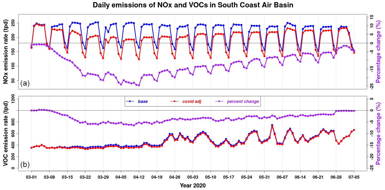
Figure 2 Daily total emissions of (a) NO_x and (b) VOCs in the South Coast Air Basin. Blue lines denote the baseline emissions, red lines denote COVID-19-adjusted emissions, and purple lines denote the percentage change in NO_x or VOCs due to the COVID-19 adjustment; the latter is calculated as follows: (COVID-19-adjusted − baseline)$/$baseline. Vertical gray dash lines correspond to Sundays.

3.1.2 Top-down: changes in ambient NO₂ after adjusting for meteorology

To validate the bottom-up emissions described in Sect. 3.1.1, we explored methods to provide a top-down estimate of the change in ambient NO₂ resulting from the COVID-19 response. The top-down estimate is complicated by the fact that changes in ambient NO₂ during 2020 are a combination of changes in meteorology, chemistry, and emissions. Historically, NO₂ concentrations in the SoCAB decrease between February and June (see Fig. 3); therefore, it is misleading to attribute the decline in NO₂ after the onset of the pandemic to emission changes alone. Furthermore, the timing of the seasonal decline in NO₂ varies from year to year, so comparison to the same month from previous years is problematic. For example, we compare the average NO₂ concentration between 20 March and 20 June in the SoCAB (based on 21 sites with data from 2015 to 2020) for 2020 with the average NO₂ from each year between 2015 and 2019. This yields a wide range of −1.5 to −4.4 ppb for ΔNO₂ in 2020, relative to previous years. We improve on this estimate by using the vehicle miles traveled (VMT) data as a predictor of activity change in order to provide a top-down estimate of the NO₂ changes that can be attributed to emissions.

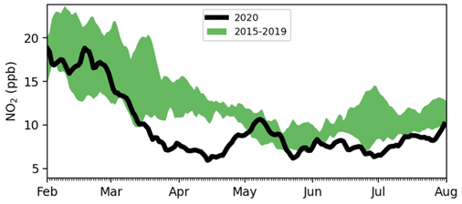
Figure 3 SoCAB pollutant concentrations for 2020 (black line) and for 2015–2019 (green shading). Data are averaged over 21 sites that contain data throughout the time period.

We construct a simple multivariate linear model to predict daily NO₂ concentrations based on relative humidity, wind speed, temperature, day of year, and day since 1 January 2016 (to capture any long-term trends). The model is trained on hourly NO₂ data from 2016 to 2019 and used to predict daily NO₂ concentrations in 2020. The model predicts daily NO₂ in 2020 well (r²=0.82, RMSE =2.3 ppb); however, the model is typically biased high from March onwards. If we include VMT as a predictor variable (still only training on 2016–2019 data), the model more closely fits the observations in 2020 (r²=0.88, RMSE =1.8 ppb). Figure 4a shows the time series of NO₂ from the observations and the model with and without VMT. In years prior to 2020, the model without VMT predicts the observed NO₂ to within 0.4 ppb, and the addition of VMT typically makes only a small difference (Fig. 4b). In 2020, the model without VMT overestimates NO₂ by 1.4 ppb relative to the observations. Including VMT provides a large correction to the model, causing it to underestimate NO₂ by −0.4 ppb. We use the bounds to estimate that the ΔNO₂ resulting from emission changes associated with the pandemic response are −1.4 to −1.8 ppb (or about 19 % to 26 %; the upper bound is the difference between the two models and assumes that the non-VMT model may overcompensate).

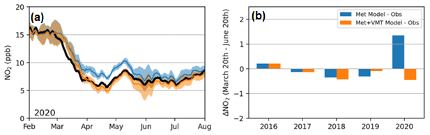
Figure 4 (a) Observed NO₂ (black) and predictions of daily NO₂ based on non-VMT variables (blue line). Uncertainty estimates are derived from the model–observation difference for the years on which the non-VMT model is trained (narrow envelope means the model performed well on the training data for that time of year). The model with VMT is shown (orange). Data have 21 d smoothing applied. (b) The average difference between the models and the observations for the period from 20 March to 20 June for each year (models are trained on 2016–2019 data).

In parallel with the multivariate model, we use the historical relationship between detrended (7 d rolling average) VMT and NO₂ to infer the ΔNO₂ resulting from the ΔVMT (−17 %) during the analysis period. The resulting ΔNO₂ via this method is −1.4 to −2.0 ppb, where the range is determined by the 95 % confidence bounds of a Theil–Sen regression of detrended VMT and NO₂. The range is almost identical to the result from comparing the multivariate model with and without VMT (discussed above). This contrasts with the estimate based on a historical comparison alone (−1.5 to −4.4 ppb) that suggests a much larger upper bound to the effect of the pandemic response on NO₂.

Finally, we compare the top-down estimate of the ΔNO₂ for 2020 with the ΔNO₂ from the 2020 CMAQ emissions inventory described in Sect. 3.1.1. The CMAQ ΔNO₂ is the difference between two simulations, which both use the same meteorology but with 2017 vs. 2020 emissions, averaged over the 21 South Coast Air Basin sites used for the top-down comparison (and the same 20 March–20 June time frame). The model produces a ΔNO₂ of −1.1 ppb when updated to 2020 emissions. This is slightly below the top-down estimation of −1.4 to −2.0 ppb. However, considering that 2020 meteorology was not used, this suggests that the 2020 emissions used for the CMAQ modeling are reasonable.

3.2 In situ and remote sensing observations

In Sect. 3.1, we quantified the changes in the O₃ precursor environment using a bottom-up and a top-down approach. These two approaches highlight that the abundance of NO_x was diminished in the April–July period of 2020, due to reductions in mobile-source emissions. This section uses satellite data and surface monitoring networks to explore how this drastic change in precursor abundances affected regional O₃ chemistry.

3.2.1 Satellite HCHO$/$NO₂ as an indicator of O₃ sensitivity

Over polluted areas, both HCHO and NO₂ have vertical distributions that are heavily weighted toward the lower troposphere, meaning that column-integrated satellite measurements of these gases are fairly representative of near-surface conditions. Many studies have taken advantage of these favorable vertical distributions to investigate surface emissions of NO_x and VOCs from space (Duncan et al., 2016; Krotkov et al., 2016; Duncan et al., 2010; Martin et al., 2004; Fishman et al., 2008). Recent literature has shown that the $\mathrm{HCHO}/{\mathrm{NO}}_{\mathrm{2}}$ ratio can be a useful indicator of regional O₃ sensitivity, although the relatively high uncertainty associated with the technique means that use of the ratio should be reserved for the qualitative evaluation of spatiotemporal trends (Schroeder et al., 2017; Jin et al., 2020). In general, very low ratios are associated with VOC-limited conditions, and very high ratios are associated with NO_x-limited conditions. In Fig. 5a, we show that the OMI $\mathrm{HCHO}/{\mathrm{NO}}_{\mathrm{2}}$ ratio in the SoCAB generally increased from 2005 to 2020. Given that previous studies had identified the SoCAB as VOC-limited during the mid-2000s, we can conclude that the increasing $\mathrm{HCHO}/{\mathrm{NO}}_{\mathrm{2}}$ ratio in Fig. 5 indicates that the SoCAB has been becoming less VOC-limited over time, which is consistent with recent literature (Pollack et al., 2012). However, this information alone is not enough to conclude whether the region had shifted to an NO_x-limited environment by the end of the time series. Figure 5b shows the detrended seasonality of the OMI $\mathrm{HCHO}/{\mathrm{NO}}_{\mathrm{2}}$ ratio from 2005 to 2020. In general, lower $\mathrm{HCHO}/{\mathrm{NO}}_{\mathrm{2}}$ ratios occurred during spring compared with summer, with the increase and plateau corresponding to the seasonality of biogenic emissions in the region (Dreyfus et al., 2002; Misztal et al., 2014). This suggests that, for a given year, spring (April–May) would appear more VOC-limited than summer (June–July) and vice versa.

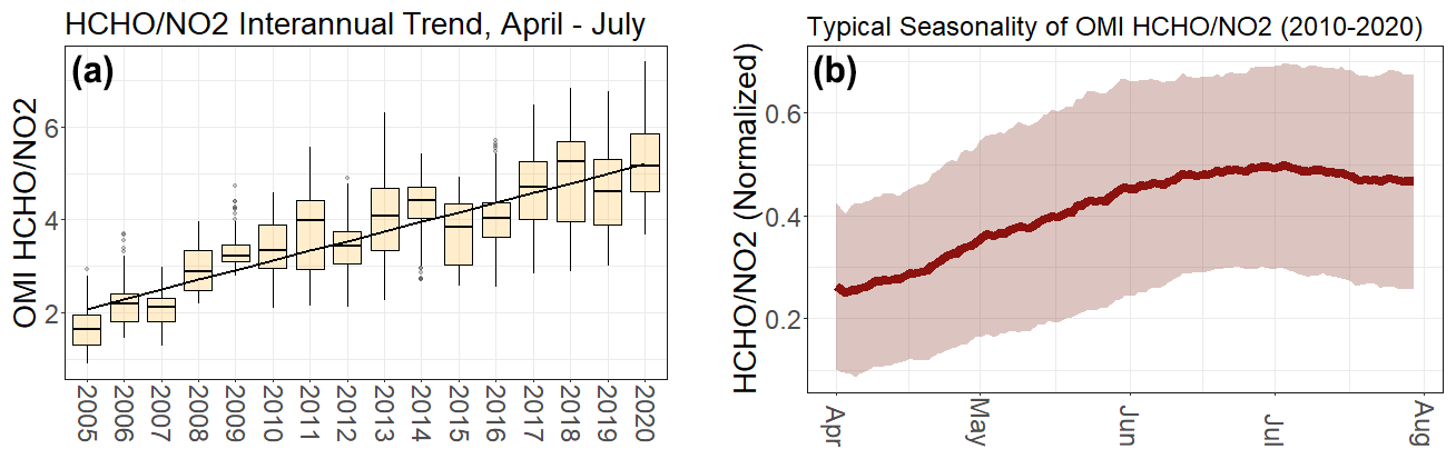
Figure 5 (a) Interannual trend in the OMI $\mathrm{HCHO}/{\mathrm{NO}}_{\mathrm{2}}$ ratio averaged over the SoCAB. Data are filtered to include the April–July period of each year. A linear fit is applied to the data. (b) Typical seasonality of OMI $\mathrm{HCHO}/{\mathrm{NO}}_{\mathrm{2}}$ averaged over the SoCAB. Data have been normalized to the range for each year.

While Fig. 5 demonstrates the qualitative utility of the $\mathrm{HCHO}/{\mathrm{NO}}_{\mathrm{2}}$ ratio for exploring interannual and seasonal trends, classification into NO_x-limited or VOC-limited regimes can be achieved by coupling this ratio with O₃ data from surface monitoring networks. Figure 6 utilizes daily $\mathrm{HCHO}/{\mathrm{NO}}_{\mathrm{2}}$ ratios (spatially aggregated over the SoCAB) coupled with daily MDA8 O₃ data from the surface monitoring network. These data are binned into 5-year increments and separated by season. When presented this way, increasing and decreasing trends within a bin can be used to identify VOC-limited vs. NO_x-limited regimes, respectively. In a region that is a firmly VOC-limited environment, $\mathrm{HCHO}/{\mathrm{NO}}_{\mathrm{2}}$ ratios are expected to have a positive relationship with MDA8 O₃ – that is, days with higher O₃ are expected to occur on days with higher $\mathrm{HCHO}/{\mathrm{NO}}_{\mathrm{2}}$ ratios (i.e., closest to the transitional regime where O₃ production is maximized along a ridgeline). In an NO_x-limited environment, the opposite would be expected, where high-O₃ days are expected to occur on days with lower $\mathrm{HCHO}/{\mathrm{NO}}_{\mathrm{2}}$ ratios (in an NO_x-limited environment, lower $\mathrm{HCHO}/{\mathrm{NO}}_{\mathrm{2}}$ ratios would be closer to the transitional state where O₃ production is maximized along a ridgeline). Using these expected tendencies as indicators, we can identify VOC-limited seasons and years, such as spring 2005–2009, summer 2005–2009, and spring 2010–2014. Spring of 2015–2019 and summer of 2010–2014 had no apparent trends (likely indicative of transitional states), whereas summer 2015–2019 showed a slight negative trend, which could be indicative of a weakly NO_x-limited photochemical regime. In contrast, both spring and summer of 2020 showed strong negative trends, with high-O₃ days associated with lower $\mathrm{HCHO}/{\mathrm{NO}}_{\mathrm{2}}$ ratios. Taken together, this implies that spring of 2020 was likely the first NO_x-limited spring season since records began, while summer likely moved from a weakly NO_x-limited regime in 2015–2019 to a firmly NO_x-limited regime in 2020.

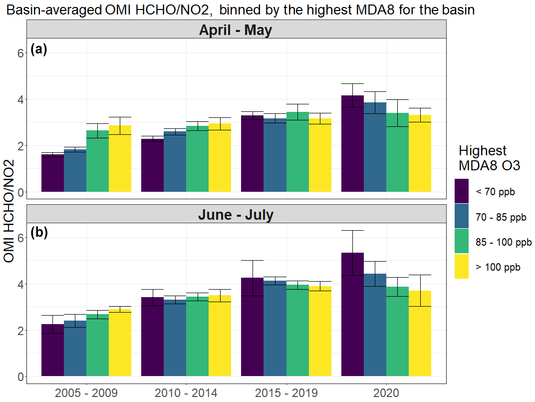
Figure 6 Time series of the basin-averaged OMI $\mathrm{HCHO}/{\mathrm{NO}}_{\mathrm{2}}$ ratios. Data are binned every 5 years and are colored by the highest MDA8 observed for the basin on each day. Each bar represents the mean ±1 standard deviation. Panel (a) shows data from spring (April–May), and panel (b) shows data from summer (June–July).

3.2.2 The O₃ weekend$/$weekday effect

While the satellite-based approach presented in Sect. 3.2.1 is useful for diagnosing O₃ sensitivity at regional scales, there are subtle nuances that cannot be accounted for using the satellite-based approach alone. First, satellite instruments, particularly OMI, have relatively coarse spatial resolution and limited utility for diagnosing subregional gradients in O₃ sensitivity. While exploring O₃ chemistry aggregated to the regional scale is certainly useful, additional information about the location of subregional gradients in O₃ sensitivity can be useful for understanding policy implications when coupled with knowledge of emission sources, population centers, and typical meteorology. Second, polar-orbiting satellites overpass once per day, typically around midday (OMI's orbit passes over California at around 13:30 LT), making it impossible to diagnose diurnal trends in O₃ sensitivity from satellite data alone. Ambient O₃ concentrations typically peak in the late afternoon and are the result of chemical production integrated over the course of the day, with midday chemistry appearing more NO_x-limited in character than other times of day (due to higher actinic flux, higher temperatures, higher biogenic emissions, and reduced NO_x emissions relative to morning and evening commute times). Applying WE$/$WD analysis to surface monitoring networks (described in Sect. 2) enables exploration of subregional gradients in O₃ chemistry. Furthermore, because this approach only employs MDA8 O₃, WE$/$WD analysis inherently contains information about the outcomes of diurnally integrated photochemistry. Figure 7 shows the long-term trend in the WE$/$WD effect in springtime (left panels) and summertime (right panels). O₃ monitor data are available prior to 2005, but the time period and binning method shown in Fig. 7 were chosen to be consistent with Fig. 6. In Fig. 7, blue colors (i.e., weekend O₃ higher than weekday O₃) are indicative of locally VOC-limited conditions, whereby reductions in NO_x on weekends coincided with higher ambient O₃. Orange colors are an indication of locally NO_x-limited conditions, whereby reductions in NO_x on weekends coincided with lower ambient O₃.

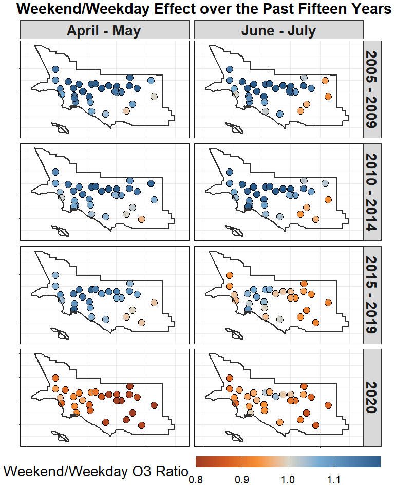
Figure 7 Time series of WE$/$WD O₃ ratios at SoCAB monitoring sites. Rows represent averages over 5-year bins, and columns represent temporal bins for spring (April–May) and summer (June–July).

In general, the trends shown in Fig. 7 agree with those presented in Sect. 3.2.1. The spring seasons of 2005–2019 appear to be VOC-limited environments, although the effect was weakening, with lighter shades of blue present in the spring seasons of 2015–2019. The analysis in Sect. 3.2.1 labeled spring 2015–2019 as transitional, whereas the analysis shown in Fig. 7 concludes that this period was likely a weakly VOC-limited environment. Summer of 2005–2014 was generally VOC-limited, with most monitors having WE$/$WD ratios below 1. However, by summer of 2015–2019, many monitoring sites had WE$/$WD ratios above 1, indicative of NO_x-limited conditions. The spatially aggregated approach employed in Sect. 3.2.1 concluded that summer 2015–2019 was a weakly NO_x-limited regime at the regional scale; however, using the WE$/$WD ratios in Fig. 7, interesting subregional gradients are noted. For example, while most sites in summer 2015–2019 had WE$/$WD ratios below 1, a concentration of monitoring sites near the urban core of Los Angeles and the Los Angeles–Long Beach corridor had WE$/$WD ratios above 1. This region is a strong source of NO_x emissions from mobile sources, including heavy-duty vehicle (HDV) traffic from the Port of Los Angeles and the Port of Long Beach. This highlights the difficulty in controlling O₃ in VOC-limited environments: urban core areas may lag the broader region in transitioning from a VOC-limited to an NO_x-limited regime, which may have important outcomes with respect to the spatial distribution of O₃ and O₃ exposure.

In spring of 2020, every monitor in the SoCAB was characterized as having WE$/$WD ratios below 1. Surprisingly, this includes the urban core of Los Angeles and the Los Angeles–Long Beach truck corridor. While O₃ chemistry in springtime is generally more VOC-limited in nature than in summertime (i.e., Fig. 5b), the deepest reductions in NO_x emissions due to COVID-19 were observed in springtime (up to a 25 % reduction; Fig. 3), implying that COVID-19-related mobile-source reductions were of a large enough magnitude to alter the springtime photochemical environment. This agrees with the satellite-based analysis presented in Fig. 6. In summertime of 2020, all but two of the monitoring sites had WE$/$WD ratios below 1. This includes the urban core of Los Angeles and the Los Angeles–Long Beach corridor, which had WE$/$WD ratios above 1 in every year prior to 2020. While summertime NO_x emissions were not reduced by as much as springtime NO_x emissions in 2020 (i.e., Fig. 2), the baseline summertime photochemistry was already weakly NO_x-limited (i.e., summer 2015–2019). This implies that the mobile-source reductions attributed to COVID-19 were sufficient to change summertime photochemistry from a weakly NO_x-limited to a firmly NO_x-limited regime, including the urban core of Los Angeles and the Los Angeles–Long Beach corridor.

3.3 Modeling results

While analysis of satellite and surface monitor data reveals that COVID-19-related NO_x reductions were sufficient to push the SoCAB into an NO_x-limited regime in both spring and summer of 2020, understanding the implications of this photochemical shift on ambient O₃ levels requires further consideration. For example, present-day satellites are only capable of measuring HCHO and NO₂ once per day, typically around midday. While these satellite data are, nonetheless, useful, one must consider that MDA8 O₃ is the result of diurnally integrated O₃ production, meaning that the current generation of satellites do not provide a complete picture. Additionally, meteorology makes interpretation of indicators difficult. It is well-documented that downwind areas in the eastern part of the SoCAB typically experience the highest MDA8 O₃ in the basin; therefore, it can be difficult to connect observed WE$/$WD ratios at receptor sites to photochemical conditions at source regions. Recent papers have analyzed spatiotemporal trends in NO₂ in the SoCAB during the COVID-19 period, and all noted that short-term meteorological variability makes it challenging to draw comparisons against recent years (Naeger and Murphy, 2020; Parker et al., 2020; Goldberg et al., 2020). Parker et al. (2020) concluded that NO_x reductions during the COVID-19 period were not associated with meaningful changes in the SoCAB O₃ concentrations; however, short-term meteorological variability can also obscure the effects that short-term changes in O₃ sensitivity impart on ambient O₃ levels. We expand upon these papers by using a compilation of chemical transport model simulations to disentangle the effects of emissions, chemistry, and meteorology on ambient O₃ levels during the study period. A statistical evaluation of the model's skill in simulating meteorological conditions across the SoCAB during the study period is provided in the Supplement. In Sect. 3.3.1 and 3.3.2, we highlight that these model simulations were able to accurately capture the long-term change in O₃ sensitivity over the past decade, and they accurately simulated the O₃ precursor environment in 2020. With this information in hand, we use two sets of simulations (the baseline case and COVID-19-adjusted emissions) to isolate and quantify the change in O₃ that can be attributed to COVID-19 precautions.

3.3.1 Multiyear simulations of the WE$/$WD effect on O₃

CMAQ has been used to simulate the Californian O₃ concentrations for 2010, 2012, 2015, 2017, and 2020 (Cai et al., 2019). The calculated WE$/$WD ratios of MDA8 O₃ from model simulations for these years are compared with the observed ratios at the monitoring sites in the SoCAB for April–July. The calculation of WE$/$WD ratios follows the procedure described in Sect. 2. The box plots in Fig. 8 show the variation in observed April–July O₃ WE$/$WD ratios among the SoCAB monitoring sites from 2000 to 2020. The solid black lines in the boxes are the mean WE$/$WD ratios of all of the sites for each year. The red dots in Fig. 8 are the modeled mean O₃ WE$/$WD ratios for the corresponding years. The 2020 modeled data are from the simulation with COVID-19-adjusted emissions. With year-by-year variations, the long-term trend in the O₃ WE$/$WD ratios shows a general decrease over the past 2 decades. Compared with the majority of the earlier years, the observed mean ratios after 2014 are much closer to 1.0, with the mean ratios for 2016, 2018, and 2020 all below 1. The model-simulated mean O₃ WE$/$WD ratios are very consistent with the observed mean ratios, indicating that the modeling system captured the change in chemical regime over the years. The difference between the modeled and observed mean ratios for 2020 is larger than the difference for the other years, with the model predicting a higher WE$/$WD ratio than observed. This may indicate that, while the model captured the transition to an NO_x-limited photochemical environment, modeled MDA8 O₃ may be slightly less sensitive to changes in NO_x than is observed. Detailed model performance comparing simulated to observed NO₂ in 2020 is shown in the following section.

Figure 8 Box plots of the observed April–July WE$/$WD ratios of MDA8 O₃ at South Coast Air Basin monitoring sites. The solid lines in each box are the mean ratios of all of the sites, and the red dots are the modeled mean ratios.

3.3.2 Model simulations for NO₂ and O₃ during the COVID-19 period

For the COVID-19 period in 2020, we analyzed times series of NO₂ and O₃ from model simulations as well as undertaking a comparison with observations from ground monitoring sites. The difference between the two model simulations with and without the COVID-19 adjustment reflects the impact of COVID-19 emission reductions. Figure 9a shows the daily average NO₂ concentrations from observations and the model simulations with COVID-19-adjusted emissions. Figure 9b shows the NO₂ difference between the two model simulations (COVID-19-adjusted – baseline emissions). As observed NO₂ at a monitoring site can be heavily impacted by the local emissions, whereas modeled data are diluted concentrations in 4×4 km² grids, we considered 18 monitoring sites that were not near roads for the NO₂ model comparison with observation. As shown in Fig. 9, the model captures the day-to-day variations in NO₂ reasonably well. The normalized mean biases of NO₂ for March, April, May, and June are −24 %, −8 %, −4 %, and 1 %, respectively. The larger model bias in March is due to the significant model underestimations during the second and third weeks of March when there was rain. The difference between simulated NO₂ using the COVID-19-adjusted emission inventory and baseline emissions shows that the NO₂ concentration was reduced by up to 2.6 ppb due to the COVID-19 emission reduction, with the maximum reduction occurring on 31 March. During April and early May, the NO₂ reduction was generally between 1 and 2 ppb. After 10 May, the reduction in NO₂ continued to become smaller and became nearly negligible by the end of June.

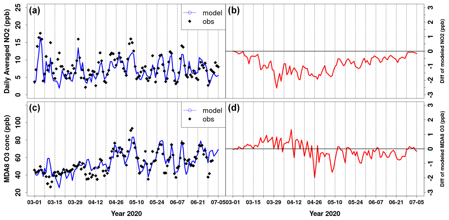
Figure 9 (a) Time series plots of daily averaged NO₂ concentrations in the South Coast Air Basin from simulations and observations. (b) Time series plots of the daily averaged NO₂ difference between the two sets of model simulations (model with the COVID-19-adjusted emission inventory minus the model with the baseline emission inventory). (c) Time series plots of averaged MDA8 O₃ concentrations in the South Coast Air Basin from simulations and observations. (d) Time series plots of the MDA8 O₃ difference between the two sets of model simulations (model with the COVID-19-adjusted emission inventory minus the model with the baseline emission inventory).

Observed and model-simulated MDA8 O₃ concentrations are shown in Fig. 9c. Larger discrepancies between modeled and observed values can be seen for the second and third weeks of March as well as the second week of April, during which time the O₃ concentrations are generally low. These two time periods were associated with two rain events, above-average cloud cover and relative humidity as well as below-average temperature. From mid-April to the end of June, when O₃ concentrations were relatively higher, modeled O₃ concentrations are in very nice agreement with the observations. A significant enhancement of O₃ was observed during late April and early May. This O₃ enhancement was successfully captured by the model except that the peak O₃ concentrations on 6 and 7 May were underpredicted by the model, consistent with the underprediction of NO₂ during these days. During late April to early May, high-pressure ridges were the dominant weather patterns over the SoCAB. The region had weak offshore winds, a low planetary boundary layer height, and extremely high temperatures, which favor the production and accumulation of O₃. The highest average daily maximum temperature from all of the monitoring sites reached 33.5 ^∘C on 6 May in both the observations and the model simulation. The O₃ difference between model simulations with COVID-19-adjusted emissions and baseline emissions is illustrated in Fig. 9d. The COVID-19 emission reduction caused the O₃ concentration to increase by up to 1.2 ppb from March to mid-April and mostly decrease by up to 2 ppb from late April to early July. On 7 May, when the highest O₃ was observed, the O₃ concentrations were reduced by about 1.7 ppb due to the COVID-19 emission reductions. The change in the O₃ difference between the two model simulations over time, especially the shift from positive to negative, indicates the transition from a VOC-limited chemical regime to a more NO_x-limited chemical regime.

4 Discussion

Using a multi-perspective approach involving satellites, surface monitors, and modeling, we show that the SoCAB was on average an NO_x-limited environment during the COVID-19 period in April–July of 2020. While satellite data and the weekend$/$weekday effect suggest that summertime in recent years may have been slightly NO_x-limited even before COVID-19-related mobile-source reductions, spring of 2020 was the first spring on record to display NO_x-limited characteristics. This outcome was achieved by relatively large emission reductions in springtime (∼20 % reduction in SoCAB NO_x emissions), which was sufficient to offset the typical climatology of O₃ sensitivity in the region. In summertime, when O₃ sensitivity is naturally more NO_x-limited than in spring (a combination of biogenic emissions, warmer temperatures, and higher actinic flux), a 5 % reduction in SoCAB NO_x emissions due to COVID-19 acted to push the region further into NO_x-limited territory. In both spring and summer of 2020, reductions in mobile-source emissions due to COVID-19-related precautions were the largest contributor to regional NO_x emission reductions. Thus, the natural experiment offered by data collected during the COVID-19 period of 2020 highlights that reductions in mobile-source emissions alone could be a feasible pathway for shifting the SoCAB into an NO_x-limited O₃ production regime.

This work builds on recent studies that focused on the impacts of COVID-19-related precautions on O₃ and its precursors in Southern California. Naeger and Murphy (2020) compared TROPOMI NO₂ levels in spring of 2020 to levels observed in spring of 2019. While the authors excluded wet periods from their analysis, the 40 % reduction that they report in Los Angeles is higher than similar studies that attempted to better account for meteorology, such as Goldberg et al. (2020), who reported a 32 % reduction in TROPOMI NO₂ for Los Angeles. In Sect. 3, our bottom-up approach using measurements of vehicle activity yielded an estimated NO_x emission reduction of 25 % during the deepest point of the shutdown, with typical reductions of ∼ 15 %–20 % during springtime and ∼5 % during summertime. While our bottom-up estimate of the reduction in NO_x emissions due to COVID-19 is lower than those reported in Naeger et al. (2020) and Goldberg et al. (2020), there are important considerations that must be made to address this discrepancy. First, both Naeger et al. (2020) and Goldberg et al. (2020) focused on city-scale observations, which included the city of Los Angeles rather than the broader SoCAB region focused on in this study. Naeger et al. (2020) showed that NO₂ reductions were strongest in the urban core; therefore, the numbers reported in Naeger (2020) and Goldberg (2020) would likely decrease if expanded to the broader SoCAB region. Second, ambient NO₂ levels are a function of both emissions and removal. As shown in this work, reduced NO_x emissions produced a fundamental shift in the underlying photochemistry of the region, which could lead to a decrease in the NO_x lifetime due to enhanced photochemical cycling. Therefore, a given decrease in the NO_x emission rate could be concurrent with an increase in the NO_x removal rate, leading to a larger observed decrease in ambient NO₂ than can be explained by emissions alone.

Recent work by Parker et al. (2020, 2022) also analyzed O₃ and its precursors in the SoCAB during the COVID-19 stay at home order. Both papers concluded that the NO_x reductions observed during that period in the SoCAB were not sufficient to reduce O₃ levels across the basin, and Parker et al. (2020) instead advocate for VOC controls in addition to NO_x reductions as a pathway for controlling O₃. Parker et al. (2022) noted an O₃ increase in the urban core of the SoCAB, which is seemingly in contrast to our work; however, when their results are averaged over the whole SoCAB (as in our work), a minor decrease in O₃ is observed. This result highlights the importance of spatial scales when considering O₃ chemistry: while we find that O₃ chemistry at the basin scale indeed shifted to an NO_x-limited regime and produced modest decreases in ambient O₃, this should not be taken to mean that these observations were uniform across the basin. The combination of our work with the work of Parker et al. (2022) suggests that future reductions in NO_x emissions will be, on average, beneficial towards reducing ambient O₃ in the SoCAB. However, this benefit may not play out evenly across the basin, and certain subregions will likely lag behind others in seeing improvements.

It should be noted that Parker et al. (2020, 2022) drew their conclusions about O₃ chemistry by focusing on the outcome (i.e., ambient O₃ concentrations) and used that to make inferences about the underlying process (i.e., O₃ chemical regime). The work presented here focuses on identifying the underlying chemical regime using process-based indicators rather than outcome-based indicators. It should be noted that, at the chemical process level, there are many scenarios where O₃ chemistry may “flip” from VOC-limited to NO_x-limited while still producing an increase in O₃ due to nonlinearities in chemistry alone, especially when dealing with air masses that are near the chemical transition point. Therefore, the observation made by Parker et al. (2022) that O₃ increased in some areas while NO_x emissions dropped is not a solid indicator of the underlying chemical regime (especially given that the SoCAB is near the chemical transition point). Our work expands upon that of Parker et al. (2022) by including the satellite $\mathrm{HCHO}/{\mathrm{NO}}_{\mathrm{2}}$ ratio as a process-based indicator of regional O₃ sensitivity and by performing model simulations with baseline case vs. COVID-adjusted emissions. While our conclusions generally agree with Parker et al. (2020, 2022), our finding that on average the SoCAB transitioned into an NO_x-limited regime in both spring and summer of 2020 cannot be understated. While reaching NO_x-limited territory is certainly not the same as reaching regional O₃ attainment, it is nonetheless an important milestone from a regulatory perspective. The fact that O₃ levels in April–July of 2020 were not particularly different from recent years does indeed suggest that NO_x reductions similar to those observed in 2020 would not be sufficient for meaningful O₃ improvements to be realized. However, our modeling experiment suggests that COVID-19-related NO_x reductions resulted in O₃ levels that were 0–2 ppb lower than they would have been in April–July in the absence of COVID-19-related precautions. The fact that the SoCAB shifted to an NO_x-limited regime and experienced a reduction in simulated O₃ (per our modeling study) emphasizes that drastic reductions in NO_x emissions (more than the reductions observed in 2020) will be effective in reducing ambient O₃ (although the response on any given day or at any given site may differ from the basin and/or seasonal average conditions). This finding is well aligned with recent state legislation, such as the Heavy-Duty Omnibus Regulation (https://ww2.arb.ca.gov/rulemaking/2020/hdomnibuslowNOx, last access: 13 September 2022) and the Governor's Executive Order mandating that all new light-duty vehicle sales be zero emission by 2035, with heavy-duty sales to follow by 2045 (https://www.gov.ca.gov/wp-content/uploads/2020/09/9.23.20-EO-N-79-20-Climate.pdf, last access: 13 September 2022). While Parker et al. (2020) is correct that concurrent reductions in VOC emissions will also be beneficial for controlling O₃, a large portion of the SoCAB VOC emissions during the O₃ season are biogenic in nature (approximately one-third or more by mass), implying that significant reductions in ambient O₃ can only be achieved with drastic reductions in NO_x emissions.

Achieving attainment for O₃ air quality standards will be further complicated by the enhanced frequency of drought and heat waves that California is expected to experience due to a changing climate (Swain et al., 2014). While short-term heat waves result in enhanced photochemical activity and are typically associated with the highest O₃ values of a season (for example, the heat wave highlighted in Sect. 3.3.2), multiyear droughts are believed to inhibit biogenic VOC emissions, which could lead to reductions in O₃ production (Demetillo et al., 2019). While this study shows that statewide efforts to drastically reduce mobile-source NO_x emissions will be effective for long-term reductions in ambient O₃ in the SoCAB, the effectiveness of such policies may be partially obscured by short-term meteorological variability and long-term climate change. Disentangling these climatic effects from the effects of regulations will be a challenge for scientists and policymakers in the next decades. Follow-up studies will likely require novel fusions of observation systems including climate models, ultrahigh-resolution chemical transport models, geostationary satellites, and dense monitoring networks.