Assessment of NAAPS-RA performance in Maritime Southeast Asia during CAMP²Ex

Monitoring and modeling aerosol particle life cycle in Southeast Asia (SEA) is challenged by high cloud cover, complex meteorology, and the wide range of aerosol species, sources, and transformations found throughout the region. Satellite observations are limited, and there are few in situ observations of aerosol extinction profiles, aerosol properties, and environmental conditions. Therefore, accurate aerosol model outputs are crucial for the region. This work evaluates the Navy Aerosol Analysis and Prediction System Reanalysis (NAAPS-RA) aerosol optical thickness (AOT) and light extinction products using airborne aerosol and meteorological measurements from the Cloud, Aerosol, and Monsoon Processes Philippines Experiment (CAMP²Ex) conducted in 2019 during the SEA southwest monsoon biomass burning season. Modeled AOTs and extinction coefficients are compared to those retrieved with a high spectral resolution lidar (HSRL-2). Agreement between simulated and retrieved AOT (R²= 0.78, relative bias $=-$5 %, normalized root mean square error (NRMSE) = 48 %) and aerosol extinction coefficients (R²= 0.80, 0.81, and 0.42; relative bias = 3 %, −6 %, and −7 %; NRMSE = 47 %, 53 %, and 118 % for altitudes between 40–500, 500–1500, and >1500 m, respectively) is quite good considering the challenging environment and few opportunities for assimilations of AOT from satellites during the campaign. Modeled relative humidities (RHs) are negatively biased at all altitudes (absolute bias $=-\mathrm{5}$ %, −8 %, and −3 % for altitudes <500 500–1500 and >1500 m, respectively), motivating interest in the role of RH errors in AOT and extinction simulations. Interestingly, NAAPS-RA AOT and extinction agreement with the HSRL-2 does not change significantly (i.e., NRMSE values do not all decrease) when RHs from dropsondes are substituted into the model, yet biases all move in a positive direction. Further exploration suggests changes in modeled extinction are more sensitive to the actual magnitude of both the extinction coefficients and the dropsonde RHs being substituted into the model as opposed to the absolute differences between simulated and measured RHs. Finally, four case studies examine how model errors in RH and the hygroscopic growth parameter, γ, affect simulations of extinction in the mixed layer (ML). We find NAAPS-RA overestimates the hygroscopicity of (i) smoke particles from biomass burning in the Maritime Continent (MC) and (ii) anthropogenic emissions transported from East Asia. This work mainly provides insight into the relationship between errors in modeled RH and simulations of AOT and extinction in a humid and tropical environment influenced by a myriad of meteorological conditions and particle types. These results can be interpreted and addressed by the modeling community as part of the effort to better understand, quantify, and forecast atmospheric conditions in SEA.

1 Introduction

Southeast Asia (SEA) has long been considered one of the most susceptible locations to the repercussions of climate change (IPCC, 2013, 2007), with the Philippines considered one of the most vulnerable in particular (Yusuf and Francisco, 2009). The Philippines is experiencing rapid urbanization, industrialization, and economic development along its extensive coastlines (Alas et al., 2018). Rising sea levels, decreased precipitation in association with the June–September southwest monsoon (SWM), prolonged droughts (Cruz et al., 2013), and increased observations of days with anomalously high rainfall (Cinco et al., 2014) all present threats to the homes, water and food security, electric needs, and livelihood of millions of people living in this area (IPCC, 2013). Additionally, tropical cyclones and their ensuing storm surges have consistently battered the Philippines (e.g., Lagmay et al., 2015). These storms may become more severe as global temperatures increase (Sobel et al., 2016; Knutson et al., 2019). Considering all these grave threats, it is more important than ever to be able to model future environmental conditions in SEA and issue timely advisories to inhabitants of the region.

Aerosol particles play a key role in the SEA regional climate and the hydrological cycle, where aerosol–cloud interactions are dictated by and, in themselves, influence atmospheric convection (e.g., Reid et al., 2012; Thornton et al., 2017; Ross et al., 2018). However, monitoring and modeling the properties, transport pathways, and chemical evolution of aerosol particles in SEA, as well as their relationships with the complex meteorology, has proven exceedingly difficult for multiple reasons, as outlined in Reid et al. (2013). Diverse natural and anthropogenic aerosol particles with dissimilar microphysical properties converge throughout the region, especially in densely populated coastal environments (e.g., Cruz et al., 2019; Hilario et al., 2020b; Kecorius et al., 2017). During the SWM, agricultural and deforestation fires as well as peat burning peak throughout much of the Maritime Continent (MC), resulting in enormous quantities of particulate and gaseous emissions that are then transported into the Philippines and northwestern tropical Pacific (NWTP). At the same time, pollution from Asia, local Philippine emissions (e.g., cooking, vehicular combustion, road dust), and ship exhaust are constantly mixed with naturally emitted aerosols, such as marine particles (e.g., sea salt (Azadiaghdam et al., 2019), organic matter, and derivatives of dimethylsulfide (DMS; Stahl et al., 2020)), dust (Cruz et al., 2019; Campbell et al., 2013), and volcanic emissions (Hilario et al., 2021). Lack of funding and various political issues have stunted efforts for routine, cohesive, and fully publicly available aerosol measurements across the region (Reid et al., 2013). Satellite retrievals are frequently impinged by nearly ubiquitous cloud cover. This shortage of reliable data has resulted in a lack of quantitative knowledge of the aerosol life cycle in this region, which has led to uncertainty in forecasting aerosol properties and their participation in regional atmospheric processes (e.g., Adler et al., 2001; Mahmud and Ross, 2005; Dai, 2006; Sun et al., 2007; Xian et al., 2009).

Reanalyses are a highly attractive tool to study and characterize the environment in SEA as they can provide consistent and widespread simulations when remotely sensed products and/or in situ observations are unavailable. Aerosol optical thickness (AOT) is one of the most common products available from aerosol models (e.g., Colarco et al., 2010; Zhu et al., 2017; Sessions et al., 2015) and reanalyses (e.g., Gelaro et al., 2017; Inness et al., 2019; Lynch et al., 2016; Randles et al., 2017; Yumimoto et al., 2017) that can be useful for inferring information about air quality (e.g., Gupta et al., 2006), visibility (e.g., Retalis et al., 2010), and particle mass concentrations (Liu et al., 2007) at a given location. AOT is also the most available and skillful aerosol property from remote sensing allowing for its retrievals to be assimilated into reanalysis models to produce a more robust product. However, the number of AOT assimilations available in and around the Philippines is limited because of the pervasive cloud cover, making model outputs of AOT subject to uncertainty for this region. In this paper, we assess performance of the Navy Aerosol Analysis and Prediction System Reanalysis (NAAPS-RA; Lynch et al., 2016) by comparing simulated AOT and aerosol extinction (the subsequent primary observable after AOT) to those retrieved with a high spectral resolution lidar (HSRL-2; Hair et al., 2008) in and around the Philippines during the Cloud, Aerosol, and Monsoon Processes Philippines Experiment (CAMP²Ex). NAAPS has been widely used and verified to understand the aerosol life cycle in SEA (Hyer and Chew, 2010; Reid et al., 2012, 2015, 2016a, b; Xian et al., 2013; Atwood et al., 2017) and its impact on clouds (Ross et al., 2018). However, its many products have not yet been simultaneously evaluated for the region.

To quantify AOT and extinction, NAAPS-RA uses simulations of speciated particle mass concentrations and relative humidity (RH) in four dimensions (three-dimensional space and time), as well as assumptions about the optical and hygroscopic properties of each particle type. Extensive vertical profiles of observed speciated particle mass concentrations, the particle hygroscopic growth parameter (γ), and RH collocated with HSRL-2 retrievals of extinction and AOT are required to thoroughly evaluate the model's outputs and identify sources of error. Such collocated profiles of mass concentrations, γ values, and HSRL-2 retrievals are limited for this campaign. However, collocated profiles of HSRL-2 retrievals and RH are widely available since (i) 193 dropsondes were released during the campaign, and (ii) dropsondes were released when the aircraft was on high-altitude legs, which means multiple HSRL-2 retrievals of extinction and AOT are typically available for locations coinciding with dropsonde releases. For this reason, we focus mainly on how replacing modeled RH profiles with dropsonde profiles affects NAAPS-RA simulations for AOT and extinction.

As discussed, a full investigation into sources of error in NAAPS-RA AOT and extinction simulations is restricted by the lack of observed column profiles of γ and speciated mass concentrations. However, we attempt to evaluate the effect of these parameters on modeled extinction coefficients for four specific case studies by confining our analysis to the mixed layer (ML) and assuming particle mass concentrations and microphysical properties are homogenous in this layer. Aircraft in situ observations of γ are substituted into NAAPS-RA to explore model performance when hygroscopic growth is quantified as accurately as possible. We also compare in situ fine and coarse particle mass concentrations to the simulated values within the ML

Knowledge from this work provides insight into how well NAAPS-RA simulates AOT and extinction in a region where data assimilations from remote sensing are limited. We then explore how errors in simulated RH may be contributing to errors in AOT and extinction outputs. The modeling community can use these findings to help confront issues in NAAPS-RA as well as to learn when simulated AOT and extinction values are most (and least) sensitive to errors in modeled RH.

2 Data and methods

2.1 Field campaign description

The CAMP²Ex field campaign (24 August to 5 October 2019; Table S1 in the Supplement) examined the effect of anthropogenic and natural aerosol particles on warm and mixed-phase precipitation in SEA during the SWM and a short post-monsoon period. The NASA P-3 aircraft carried out 19 research flights (RFs) equipped with a payload of instruments and remote sensors to sample the microphysical, hydrological, dynamical, thermodynamic, and radiative properties of the environment in and around the Philippines. Specific air masses sampled include long-range transport of peat burning and pollution from Borneo, Asian pollution, Philippine outflow, and cleaner marine conditions (Hilario et al., 2021). Some of the specific interests include (i) investigating relationships between aerosol particle properties (e.g., number concentrations, composition, and spatial distribution) and shallow cumulus and congestus cloud features (e.g., optical properties, microphysical properties, and their transition from shallow to deep convection), (ii) assessing how the region's meteorology both influenced and was influenced by aerosol–cloud interactions, and (iii) developing remote sensing, modeling, and technology advances to improve regional monitoring and Earth system assessment. The flight strategy consisted of (i) identifying and flying to locations with opportune meteorological conditions and/or air masses (e.g., smoke advecting from the MC, East Asian outflow); (ii) beginning with a high-altitude leg (∼ 6–8 km) at the location of interest so that remote sensors (e.g., the HSRL-2) and any released dropsondes could inform of noteworthy environmental features below the aircraft; and (iii) flying to identified features to sample the relevant aerosol field, cloud properties, and environmental conditions.

2.2 Airborne in situ measurements

The P-3 carried a comprehensive package of instruments for quantifying aerosol particle properties, cloud properties, and meteorology. Here we discuss the instrument observations relevant to this study. Dropsonde data provided vertical profiles of RH, while a condensation particle counter (CPC; TSI-3756) supplied number concentrations for particles with diameters greater than 3 nm (Table 1). Two nephelometers (TSI-3563) in parallel (Anderson and Ogren, 1998) provided the hygroscopic growth parameter (γ; 550 nm) used to calculate the hygroscopic scattering enhancement factor (f(RH); Ziemba et al., 2013). An Aerodyne high-resolution time-of-flight aerosol mass spectrometer (AMS; Canagaratna et al., 2007; Decarlo et al., 2006) provided nonrefractory, chemically resolved aerosol particle mass concentrations for particles with diameters of 60–600 nm for the following species: organic aerosol (OA), sulfate (SO${}_{\mathrm{4}}^{\mathrm{2}-}$), nitrate NO${}_{\mathrm{3}}^{-}$), ammonium (NH${}_{\mathrm{4}}^{+}$), and chloride (Cl⁻). The AMS was operated in 1 Hz fast mass spectral (MS) mode, with final data averaged to 30 s time resolution. A fast cloud droplet probe (FCDP; SPEC Inc.; Glienke and Mei, 2020; SPEC 2013, 2019) supplied size distribution data for cloud droplets and aerosol particles with diameters of 1.5–50 µm. Data from the FCDP and a two-dimensional stereo cloud probe (2D-S10; Spec Inc.; Lawson et al., 2006) were integrated to create a cloud buffer product (SPEC Inc.) that flags when the P-3 flew through clouds as well as the 3 s before and after each pass through a cloud.

Table 1 Summary of datasets used in this study. “n/a” stands for not applicable.

*Data were only used if they were collected during isokinetic sampling and when the cloud buffer product indicated clear conditions. ^a Based on a nominal aircraft speed of 100 m s⁻¹. ^b Brechtel Manufacturing Inc. Model 1204 CVI . ^c University of Hawaii/Clarke-style shrouded solid diffuser inlet. ^d “ABF” stands for anthropogenic and biogenic fine species.

When the aircraft entered clouds, a counterflow virtual impactor (CVI) inlet (Shingler et al., 2012) was used to sample droplet residual particles. In cloud-free air, ambient aerosol particles were sampled continuously through an isokinetic Clarke-style shrouded solid diffuser inlet (McNaughton et al., 2007). Data used in this study were filtered to isolate those collected during isokinetic sampling and when the cloud buffer indicated clear conditions.

2.3 HSRL-2 retrievals and derived products

A HSRL-2 (Hair et al., 2008; Burton et al., 2018) retrieved total AOT as well as cumulative AOT (15 m vertical resolution) at 355 and 532 nm, as well as integrated backscatter and retrieved extinction at 1064 nm. Cumulative AOT is reported so that values increase as altitude decreases. Thus, the cumulative AOT reported at the lowest altitude should match the total AOT value for that particular column retrieval.

This study focuses on retrievals at 532 nm to provide the most impactful model evaluation. As will be discussed in Sect. 2.4, NAAPS-RA is a bulk model that can output AOT at over 2 dozen wavelengths. Functionally, these wavelengths are coupled to 550 nm, which is a widely used wavelength in aerosol modeling and satellite remote sensing. Although we calculate model outputs at 532 nm, key findings from this work are still relevant to NAAPS-RA simulations at 550 nm. Given this and that extinction and AOT are retrieved with the HSRL-2, we focus on the benchmark green wavelength in this study.

The HSRL-2 mixed-layer-height (MLH) product is derived from HSRL-2 backscatter profiles at 532 nm using the method described in Scarino et al. (2014). We averaged all available MLHs for each RF and proceeded to use these average heights (Table S2) in several ways throughout the rest of the analysis. For example, the lowest average MLH (∼ 500 m) was used to filter retrieved and simulated extinction coefficients to evaluate NAAPS-RA performance strictly within the ML across the campaign. Additionally, we used the average MLH for each case study to isolate airborne measurements made exclusively within this layer. The case studies will be discussed in greater detail below.

2.4 NAAPS-RA AOT and extinction products

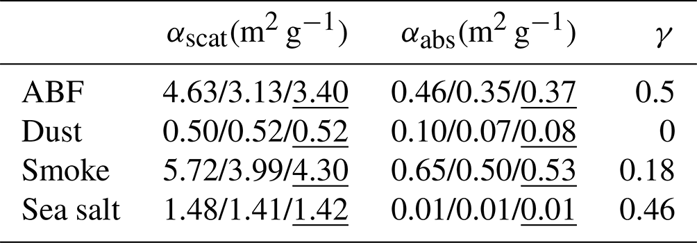
In response to the pressing need for an aerosol reanalysis product with widespread spatial and temporal coverage, the U.S. Naval Research Laboratory developed NAAPS with multiple configurations for operations, reanalyses (Lynch et al., 2016, and references therein used here), and ensembles (Rubin et al., 2016). The reanalysis version, NAAPS-RA, is an aerosol model intended for basic research including the creation of long and consistent data records. NAAPS-RA is an offline chemical transport model with a 6 h temporal resolution, 1^∘ × 1^∘ spatial resolution, 25 vertical levels based on a terrain-following sigma-pressure coordinate system, and meteorological fields that are driven by the Navy Global Environmental Model (NAVGEM; Hogan et al., 2014). Lynch et al. (2016) provide a full description of NAAPS-RA, but in short it is a chemical transport model simulating the four-dimensional distribution of four externally mixed aerosol species, dust, sea salt (both of which are dominated by coarse-mode (>1 µm) particles), open biomass burning smoke, and a combined anthropogenic and biogenic fine (ABF) species, that incorporates secondarily produced species such as sulfate and organics (both of which are dominated by fine-mode particles [(<1 µm)). Aerosol properties for each species are defined in bulk and specific size distributions are not considered.

NAAPS-RA optical properties are defined using species-dependent mass scattering and absorption efficiencies (α_scat, and α_abs, respectively) and the Hänel (1976) formulation of the light scattering hygroscopic growth function f:

$$\begin{array}{}\text{(1)}& \begin{array}{rl}& b_{\mathrm{scat},i}\left(\mathit{\lambda },x,y,z\right)\\ & =c_i\left(x,y,z\right){\mathit{\alpha }}_{\mathrm{scat},i}\left(\mathit{\lambda }\right)f_i\left[\mathrm{RH}\left(x,y,z\right)\right]\end{array}\end{array}$$

$$\begin{array}{}\text{(2)}& f_i\left[\mathrm{RH}\left(x,y,z\right)\right]={\left[{\displaystyle \frac{\mathrm{100}-\mathrm{RH}}{\mathrm{100}-{\mathrm{RH}}_o}}\right]}^{-{\mathit{\gamma }}_i}\end{array}$$

$$\begin{array}{}\text{(3)}& b_{\mathrm{abs},i}\left(\mathit{\lambda },x,y,z\right)=c_i\left(x,y,z\right){\mathit{\alpha }}_{\mathrm{abs},i}\left(\mathit{\lambda }\right)\end{array}$$

$$\begin{array}{}\text{(4)}& \begin{array}{rl}{b}_{\mathrm{ext},i}\left(\mathit{\lambda },x,y,z\right)& =b_{\mathrm{scat},i}\left(\mathit{\lambda },x,y,z\right)\\ & +b_{\mathrm{abs},i}\left(\mathit{\lambda },x,y,z\right)\end{array}\end{array}$$

$$\begin{array}{}\text{(5)}& {\mathit{\tau }}_i\left(\mathit{\lambda },x,y\right)=\int b_{\mathrm{ext},i}\left(\mathit{\lambda },x,y,z\right)\mathrm{d}z\end{array}$$

$$\begin{array}{}\text{(6)}& \mathit{\tau }\left(\mathit{\lambda },x,y\right)=\sum _{i=\mathrm{1}}^{\mathrm{4}}{\mathit{\tau }}_i\left(\mathit{\lambda },x,y\right).\end{array}$$

Here, b_scat,i, b_abs,i, and b_ext,i are the scattering, absorption, and extinction coefficients, respectively, at a given wavelength (λ), and c_i is the mass concentration of species i. The horizontal coordinates (xy) represent the longitudinal and latitudinal dimensionality (m), respectively, of each 1^∘ × 1^∘ grid cell, while z (m) is the midpoint altitude of a given pressure layer. Each pressure layer has a unique thickness dz that increases with altitude. For f(RH), RH is the humidified relative humidity, RH_o is a dry reference relative humidity (30 %), and γ_i is an empirical species-dependent hygroscopic growth parameter.

Vertical integrals then provide the speciated optical depths τ_i, which are then added to obtain total optical depth τ. Quality-controlled and assured Moderate Resolution Imaging Spectroradiometer (MODIS) and Multi-angle Imaging SpectroRadiometer (MISR) AOT data (Zhang and Reid, 2006; Hyer et al., 2011; Shi et al., 2011) are assimilated through the Navy Atmospheric Variational Data Assimilation System (NAVDAS) for AOT (NAVDAS-AOT; Zhang et al., 2008) into the model to create a final reanalysis product. When MODIS AOT data are assimilated into NAAPS, τ_i is adjusted proportionally for each species. Corrections in τ_i are converted to changes in c_i using the optical properties for that species and the simulated meteorological conditions (e.g., RH).

Frequent cloud cover over SEA often interferes with satellite retrievals of AOT for the region. Thus, it is unsurprising that <10 quality-controlled and assured MODIS retrievals were assimilated into NAAPS-RA per 1^∘ × 1^∘ grid cell for the region over the 6-week period relevant to the campaign (Fig. S1 in the Supplement). This was far fewer assimilations compared to other locations of the world yet consistent with other regions located along the intertropical convergence zone (ITCZ). The accuracy of these AOT and extinction simulations can only be determined by verification with other retrievals (e.g., AOT retrievals from the Aerosol Robotic Network (AERONET)). For example, uncertainties in AERONET AOT retrievals are reported as <0.02 (Dubovik et al., 2000; Eck et al., 1999), and so the lowest AOT that NAAPS-RA can accurately represent is ∼ 0.01.

As mentioned above, NAAPS-RA can output AOT at multiple wavelengths, including 450 and 550 nm. To simulate NAAPS-RA AOT and extinction at 532 nm, we interpolated aerosol optical properties to 532 nm (Table 2) and used these values in Eqs. (1) and (3).

Table 2 Optical properties for the four aerosol types considered in NAAPS-RA at three wavelengths (450/550/532 nm). NAAPS-RA optical properties are defined at 450 and 550 nm, and these were used to interpolate values for 532 nm, which are underlined below. Optical properties are based on the software package OPAC (Optical Properties of Aerosols and Clouds; Hess et al., 1998) at various wavelengths for ABF species, dust, and sea salt. Smoke optical properties are based on Reid et al. (2005). “ABF” stands for anthropogenic and biogenic fine species.

2.5 Strategy to evaluate NAAPS-RA performance

2.5.1 Isolating HSRL-2 data for locations of interest

The main objective of this work is to investigate how correcting errors in simulated RH affects model outputs for AOT and extinction. NAAPS-RA AOT and extinction simulations were only evaluated for the 1^∘ × 1^∘ grid cells encompassing dropsonde release points (Fig. S2). To establish the “ground truth” dataset, HSRL-2 retrievals were extracted if they occurred anywhere within a 1^∘ × 1^∘ grid cell containing a dropsonde release. These retrievals were then filtered using the cloud buffer product to ensure the P-3 was not flying in cloudy conditions, while the HSRL-2 simultaneously retrieved data from below the plane. The remaining retrievals were filtered further to isolate retrievals obtained only when the P-3 was flying at a level altitude so that data were eliminated if the aircraft was either ascending or descending. Retrievals of total AOT remaining after these steps comprised the ground truth AOT dataset. Remaining retrievals of cumulative AOT were filtered one last time to eliminate cumulative AOT values with anomalously high absolute values.

2.5.2 NAAPS-RA data considerations

NAAPS-RA reports simulated values at the center of each 1^∘ × 1^∘ grid cell, and these simulations are intended to represent the average conditions within that grid cell. This is problematic as the P-3 often only flew through sections of a 1^∘ × 1^∘ grid cell, which means the in situ data are not representative of the entire grid cell. To promote a fair comparison, NAAPS-RA model data for speciated mass concentrations and RH were interpolated to each location corresponding to a single HSRL-2 retrieval as well as to each location of a dropsonde release.

NAAPS-RA 532 nm extinction and AOT values were calculated using Eqs. (1)–(4) and (1)–(6), respectively, using the interpolated mass concentrations, interpolated RH values, and speciated 532 nm optical properties. For each AOT calculation, the lower bound of the integral in Eq. (5) corresponded to the lower range of the HSRL-2 cumulative AOT product (∼ 40 m) while the upper bound corresponded to the highest altitude at which the HSRL-2 cumulative AOT product was reported at that location. The P-3 did not typically fly above 8 km, and HSRL-2 retrievals of cumulative AOT were typically unavailable for altitudes above 6 km. Thus, these calculated NAAPS-RA AOTs and extinction coefficients are only representative of the model's 2nd–16th pressure layers.

2.5.3 Spatial averaging

Remotely sensed data were averaged first vertically and then horizontally to match the resolution of the NAAPS-RA model. HSRL-2 cumulative AOT values falling within the altitude bounds of each pressure layer were grouped. The cumulative AOT at the top of the pressure layer was subtracted from the value reported at the bottom of the pressure layer to establish a “slab” AOT for that pressure layer. This slab AOT was divided by the thickness of the pressure layer to achieve an extinction coefficient representative of that layer and for that specific vertical column. Calculated extinction coefficients for the same pressure layer were combined across all available column retrievals within the same 1^∘ × 1^∘ grid cell and averaged to arrive at a single vertical profile of extinction representing that 1^∘ × 1^∘ grid cell. Interpolated NAAPS-RA extinction coefficients within this same grid cell were horizontally averaged in an identical fashion (e.g., all interpolated coefficients for the first pressure layer were combined and averaged). The result was an average ground truth HSRL-2 extinction profile and NAAPS-RA extinction profile for the same 1^∘ × 1^∘ grid cell that could then be compared. All HSRL-2 total AOT values available within a grid cell were averaged to produce a ground truth AOT for that grid cell. Calculated NAAPS-RA AOT values were also averaged to arrive at a single simulated AOT value representative of the same portion of the grid cell.

The number of dropsondes released within a single 1^∘ × 1^∘ grid cell ranged from one to six. All dropsonde data available within a grid cell were combined, grouped, and averaged to produce a single RH value corresponding to each NAAPS-RA pressure layer. NAAPS-RA RH profiles interpolated to each dropsonde release were also combined and averaged to arrive at a single RH profile that could then be compared to the averaged in situ profile.

2.5.4 Comparison and model refinement

To explore NAAPS-RA performance as a function of altitude, we compare extinction coefficients within three altitude layers: (i) 40–500 m, (ii) 500–1500 m, and (iii) above 1500 m. The first altitude layer indicates how well NAAPS-RA simulates extinction within the ML (as discussed in Sect. 2.3), the second informs how well NAAPS-RA simulates the transition from the ML to the free troposphere (FT), and the third altitude layer focuses on model performance exclusively in the FT.

We begin by comparing HSRL-2 and NAAPS-RA extinction coefficients and AOT when NAAPS-RA values were calculated with modeled RHs to establish a basic understanding of model performance without any substitutions of in situ data. The average dropsonde RH profile for each grid cell was then used to recalculate all NAAPS-RA extinction coefficients and AOT values within that same 1^∘ × 1^∘ grid cell. The recalculated values are compared to the same HSRL-2 retrievals for that grid cell to understand how correcting errors in modeled RH affected NAAPS-RA simulations for AOT and extinction. The coefficient of determination (R²), bias, relative bias, root mean square error (RMSE), and normalized RMSE (NRMSE) are used to evaluate all NAAPS-RA simulations using the following formulations:

$$\begin{array}{}\text{(7)}& R^{\mathrm{2}}={\left[{\displaystyle \frac{\mathrm{1}}{N-\mathrm{1}}}\sum _{i=\mathrm{1}}^N\left[{\displaystyle \frac{X_i-\stackrel{\mathrm{‾}}{X}}{(X_i-\stackrel{\mathrm{‾}}{X}{)}^{\mathrm{2}}}}\right]\left[{\displaystyle \frac{Y_i-\stackrel{\mathrm{‾}}{Y}}{(Y_i-\stackrel{\mathrm{‾}}{Y}{)}^{\mathrm{2}}}}\right]\right]}^{\mathrm{2}}\end{array}$$

$$\begin{array}{}\text{(8)}& \mathrm{bias}=\sum _{i=\mathrm{1}}^N{\displaystyle \frac{Y_i-X_i}{N}}\end{array}$$

$$\begin{array}{}\text{(9)}& \mathrm{relative}\mathrm{bias}={\displaystyle \frac{\mathrm{bias}}{\stackrel{\mathrm{‾}}{X}}}\end{array}$$

$$\begin{array}{}\text{(10)}& \mathrm{RMSE}=\sqrt{\sum _{i=\mathrm{1}}^N{\displaystyle \frac{{\left(Y_i-X_i\right)}^{\mathrm{2}}}{N}}}\end{array}$$

$$\begin{array}{}\text{(11)}& \mathrm{NRMSE}={\displaystyle \frac{\mathrm{RMSE}}{\stackrel{\mathrm{‾}}{X}}},\end{array}$$

where X and Y are a set of in situ observations and NAAPS-RA simulations, respectively, for the same parameter (e.g., AOT, extinction, RH); N is the total number of points for a given comparison; and $\stackrel{\mathrm{‾}}{X}$ and $\stackrel{\mathrm{‾}}{Y}$ are the mean of sets X and Y, respectively.

2.6 Case studies

As mentioned above, the Philippines region is influenced by a range of aerosol types (Hilario et al., 2021). Aerosol models, such as NAAPS-RA, are heavily parameterized and are often challenged by the properties of individual air masses. To provide context to the bulk comparisons, four case studies were examined to assess model sensitivity and performance across a diverse range of aerosol conditions. We focus on model performance in the ML for a single 1^∘ × 1^∘ grid cell for each of the four case study flights. We assume fine and coarse particle mass concentrations and particle microphysical properties (i.e., γ) are uniform at all altitudes within the ML, which allows us to bypass the issue that vertical profiles of these parameters were infrequent during CAMP²Ex.

Airborne observations from the AMS, FCDP, and nephelometers were filtered to isolate data collected below the average MLH for each case study flight. We identified the 1^∘ × 1^∘ grid cell with the most available data for these variables, and this became the grid cell used to represent a particular case study. These flights and their respective grid cells are introduced below. Note that the monsoonal transition occurred from 23–24 September 2019.

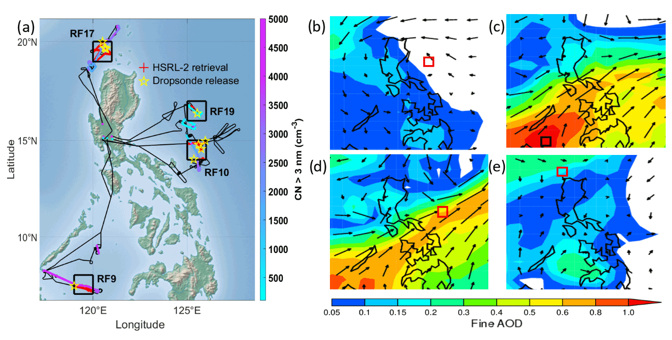
Figure 1 Relevant spatial information for the four case studies including (a) flight tracks (black lines), grid cells selected to represent each case study (black squares), and locations where HSRL-2 retrievals were available (red crosses) and dropsondes were released (yellow stars) within the selected grid cells. Flight tracks are colored by particle number concentrations (i.e., condensation nuclei (CN)) observed at altitudes within the ML. Simulations of NAAPS-RA fine aerosol optical depth (AOD) and 925 mbar wind speed are shown for the 6 h periods most relevant to (b) Case I on 5 October 2019 (RF19), (c) Case II on 15 September 2019 (RF9), (d) Case III on 16 September 2019 (RF10), and (e) Case IV on 1 October 2019 (RF17). White coloring indicates a fine AOD of ∼ 0. Red squares indicate the 1^∘ × 1^∘ grid cell relevant to each case study (a black square is used for Case II).

2.6.1 Case study descriptions

1. Case I: background marine (RF19: 5 October 2019). The location and relatively low observed and simulated aerosol particle loadings indicate the P-3 sampled a relatively clean marine environment as compared to the rest of the campaign during this flight and within the selected grid cell (Fig. 1).

2. Case II: biomass burning smoke (RF9: 15 September 2019). Flight notes, photographs, and chemistry from RF9 reveal exceptionally hazy/smoky conditions. The location and timing of this flight and selected grid cell were conducive to sampling smoke transported from the MC that had been aging for 2–3 d (Fig. S3).

3. Case III: biomass burning smoke with additional aging (RF10: 16 September 2019). The P-3 sampled the same air mass encountered during RF9 with the important difference that the smoke had aged an additional ∼ 24 h as it advected from the Sulu Sea into the Philippine Sea.

4. Case IV: Asian pollution (RF17: 1 October 2019). The aircraft sampled relatively high concentrations of SO${}_{\mathrm{4}}^{\mathrm{2}-}$ (∼ 8 µg m⁻³; measured with the AMS) in the ML during this flight. The location of the flight track and selected grid cell in relation to simulated wind patterns at 925 hPa make it reasonable to assume the enhanced SO${}_{\mathrm{4}}^{\mathrm{2}-}$ was from East Asian outflow (e.g., Lim et al., 2018; Hilario et al., 2021).

2.6.2 Case study comparison and model refinement

Mixed-layer AOT (AOT_ML) is the metric used to evaluate NAAPS-RA performance for the case study analysis. The HSRL-2 cumulative AOT value at the altitude closest to the average MLH for each case study flight was subtracted from the cumulative AOT value at the lowest altitude (40 m) to determine AOT_ML for each retrieval available within the case study 1^∘ × 1^∘ grid cell. The average of all retrieved AOT_ML values became the ground truth AOT_ML for a given case study. NAAPS-RA extinction coefficients calculated with modeled RHs (Sect. 2.5.2) were used in Eq. (5) to calculate AOT_ML at all locations coinciding with HSRL-2 retrievals. In these integrals, the lower bound was again 40 m, while the upper bound was the average MLH for a given case study flight. The calculated AOT_ML values were averaged to produce a single NAAPS-RA AOT_ML when only modeled parameters were used. This procedure was repeated with the NAAPS-RA extinction coefficients calculated using dropsonde RHs (Sect. 2.5.4) to arrive at a NAAPS-RA AOT_ML when only errors in model RH had been corrected.

Next, observed γ values and modeled RHs were used in Eq. (2) to calculate NAAPS-RA AOT_ML values when only γ was corrected. To account for the range of in situ γ values observed during a given case study, the mean γ as well as γ values 1 standard deviation above and below the mean were used in Eq. (2), resulting in a range of NAAPS-RA AOT_ML outputs. Normally, NAAPS-RA uses a species-dependent γ_i value in Eq. (2) to calculate f(RH) for each of the four aerosol types. Here, we use the same in situ γ in Eq. (2) for all four aerosol types. A mean mass-weighted NAAPS-RA γ was calculated for each case study using average mass fractions of ABF species, dust, smoke, and sea salt particles in the ML multiplied by their respective γ_i value. Comparing the NAAPS-RA mean mass-weighted γ to statistics for the in situ γ observations provides insight into how accurately the model simulated particle hygroscopicity for each case study.

Observed γ and dropsonde RH values were then both used in Eq. (2) to produce NAAPS-RA AOT_ML values when the entire f(RH) term had been corrected. After correcting this term, remaining discrepancies between modeled and retrieved AOT_ML values are presumably due to errors in simulated particle mass concentrations and/or the mass scattering and absorption efficiencies assigned to each particle type.

It is challenging to evaluate simulated mass concentrations of ABF species, dust, smoke, and sea salt particles and their respective optical properties because these particle type categories do not align with what was measured on the aircraft. For example, the AMS can quantify mass concentrations of organics, but it is difficult to determine the fraction of these organics associated with smoke versus the fraction associated with anthropogenic and/or biogenic emissions (which NAAPS-RA would place in the ABF category). To bypass this issue, we only compared simulated fine and coarse particle mass concentrations to in situ observations. NAAPS-RA fine mass was calculated as the sum of ABF and smoke mass, while coarse mass was calculated as the sum of dust and sea salt mass. The method to derive in situ fine and coarse particle mass concentrations is described below.

2.6.3 In situ mass concentrations

Eqs. (1) and (3) show that dry particle mass concentrations are an important component in simulating particle light extinction. Fine and coarse in situ mass concentrations were calculated to compare to those simulated by NAAPS-RA in the ML for each case study. In situ fine mass was characterized as the sum of AMS mass concentrations for OA, SO${}_{\mathrm{4}}^{\mathrm{2}-}$, NO${}_{\mathrm{3}}^{-}$, NH${}_{\mathrm{4}}^{+}$, and Cl⁻. Previous studies have examined the ability of the AMS to capture total fine particle mass by comparing to fine mass concentrations derived with other instruments, such as particle-into-liquid samplers (PILSs; e.g., Takegawa et al., 2005), optical particle counters (OPCs; e.g., Middlebrook et al., 2012, and references therein), and tapered element oscillating microbalances (TEOMs; e.g., Salcedo et al., 2006). AMS collection efficiency (CE) is adjusted to reach mass closure with the aforementioned and related instruments, with a CE of 0.5 being most common (Middlebrook et al., 2012, and references therein). AMS CE was set to 1 for the campaign based on comparison with coincident PILS measurements. This, in conjunction with the instrument's insensitivity to submicron dust and sea salt, indicates AMS mass concentrations represent a lower limit of true dry fine mass.

Coarse particle mass concentrations were calculated using FCDP size distributions and assuming all coarse particles were sea salt. In support of this, Hilario et al. (2020a) found crustal-marine particles to contribute 57 % of the coarse particle mass (1.15–10 µm) in the South China Sea in late September. As the FCDP sampled particles under ambient conditions, the dry particle diameter (D_p) range was calculated for each bin using the procedure described in Lewis and Schwartz (2004; see pages 54–55). Specifically, equations modeling the deliquescence growth curve for sea salt were used to determine relationships between the radii of sea salt particles at ambient RH (r), at 80 % RH (r₈₀), and in dry conditions (r_dry):

$$\begin{array}{}\text{(12)}& {\displaystyle \frac{r}{r_{\mathrm{80}}}}={\displaystyle \frac{\mathrm{0.54}}{{\left(\mathrm{1}-\mathrm{RH}\right)}^{\frac{\mathrm{1}}{\mathrm{3}}}}}\mathrm{for}\mathrm{RH}>\mathrm{93}\mathit{\%}\text{(13)}& {\displaystyle \frac{r}{r_{\mathrm{80}}}}={\displaystyle \frac{\mathrm{0.67}}{{\left(\mathrm{1}-\mathrm{RH}\right)}^{\frac{\mathrm{1}}{\mathrm{4}}}}}\mathrm{for}\mathrm{RH}<\mathrm{93}\mathit{\%}\text{(14)}& {\displaystyle }{r}_{\mathrm{dry}}={\displaystyle \frac{r_{\mathrm{80}}}{\mathrm{2}}}.\end{array}$$

For each FCDP size distribution, radii marking the edges of each size bin were set equal to r, while airborne meteorological data provided temporally coincident ambient RH values. The dry size distributions were then integrated using the density of sea salt (2.20 g cm⁻³; Seinfeld and Pandis, 2016) to arrive at total dry coarse particle mass concentration.

There are several uncertainties associated with quantifying coarse mass this way. First, this correction is very sensitive at RH >∼ 90 %, where sea salt exhibits large growth factors (e.g., Lewis and Schwartz, 2004). RHs above this threshold were common in the ML throughout the campaign (as will be shown in Sect. 3.2). The resulting large differences between ambient and dry particle radii corresponded to even larger corrections for dry particle volume and, therefore, dry particle mass. Additionally, there are known challenges in using OPCs (such as the FCDP) to accurately quantify coarse particle mass concentrations. The FCDP assumes the refractive index of water to derive sizes for all particles it samples, which introduces error when particles are not predominantly liquid. However, it is inconclusive as to whether coarse mass concentrations derived from OPCs tend to be negatively or positively biased. For example, Reid et al. (2003, 2006) found coarse-mode OPCs to overestimate the size of coarse particles (e.g., sea salt and dust), while other works have found OPCs to underestimate coarse mass concentrations (Kulkarni and Baron, 2011; Burkart et al., 2010). Our derived fine and coarse masses are still useful in roughly evaluating the corresponding NAAPS-RA simulations, but this analysis is highly preliminary and requires further investigation.

3 Results and discussion

3.1 AOT and extinction comparison using NAAPS-RA RHs

Over the course of 19 RFs, the P-3 sampled a wide variety of aerosol and meteorological conditions, which provides an opportunity to evaluate the model against a variety of atmospheric conditions. Air masses and aerosol features encountered include both clean and smoky conditions over the Sulu Sea (RFs 4 and 9, respectively), relatively clean conditions as well as aged smoke over the Western Pacific (RFs 19 and 10, respectively), East Asian outflow (RFs 11, 13, 14, and 17), shipping emissions (e.g., RF16), emissions from a coal-fired power plant (RF8), and brief samplings over the Mayon Volcano (RF10). The aircraft also encountered land breezes, cold pools, convective cells, confluence and convergence lines, and convective outflow bands from a tropical cyclone, as well as fair weather.

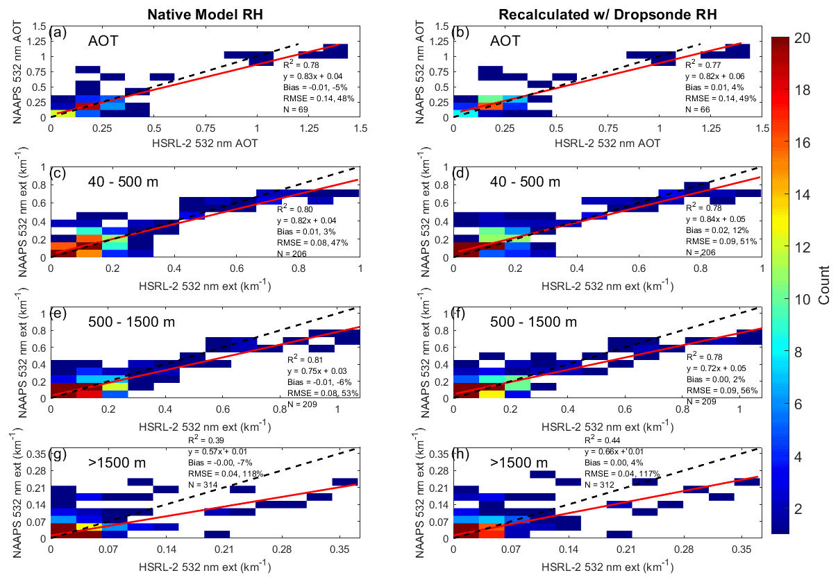
Figure 2 Comparison between simulated (NAAPS-RA) and retrieved (HSRL-2) (a and b) 532 nm aerosol optical thickness (AOT) as well as 532 nm extinction coefficients (c and d) between 40–500 m, (e and f) between 500–1500 m, and (g and h) above 1500 m. Left-hand panels are for NAAPS-RA simulations using modeled relative humidities (RHs), and right-hand panels are for simulations using dropsonde RHs. Linear fits are indicated with red lines, 1:1 lines are shown as dotted lines, and the color bar indicates the number of points falling in each bin. Where bias and RMSE are reported, the first and second numbers are the absolute and relative values, respectively.

Overall, NAAPS-RA displays good agreement with HSRL-2 retrievals for AOT (R²= 0.78, relative bias $=-\mathrm{5}$ %, NRMSE = 48 %; Fig. 2). However, it is worth noting that there is scatter between observed and simulated AOT at low AOT where NAAPS-RA can be off by a factor of 2 to 3 in some cases. Extinction coefficient analyses provide insight into the model's performance in the vertical dimension. NAAPS-RA shows the best agreement with HSRL-2 retrievals for extinction within the first two altitude layers (i.e., from 40–500 m (R²= 0.80, relative bias = 3 %, NRMSE = 47 %) and from 500–1500 m (R²= 0.81, relative bias $=-\mathrm{6}$ %, NRMSE = 53 %)). A lower R² value (0.39) and higher NRMSE (118 %) indicate agreement decreases above 1500 m, but the relative bias (−7 %) is similar to other altitude layers. Although agreement appears to decrease, absolute differences between simulated and retrieved extinction coefficients are not necessarily larger above 1500 m than differences at lower altitudes (Fig. S4).

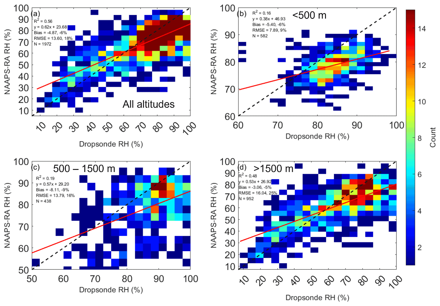
Figure 3 Comparison between simulated (NAAPS-RA) and measured (dropsonde) RH (a) for all altitudes, (b) below 500 m, (c) between 500–1500 m, and (d) above 1500 m. Linear fits are indicated with red lines, 1:1 lines are shown as dotted lines, and the color bar indicates the number of points falling in each bin. Where bias and RMSE are reported, the first and second numbers are the absolute and relative values, respectively.

3.2 AOT and extinction comparison using dropsonde RHs

We expected to see noticeable changes in extinction agreement after substituting dropsonde RHs (i) due to poor agreement between NAAPS-RA RHs and dropsonde RHs at all altitudes (R²= 0.56, relative bias $=-\mathrm{6}$ %, NRMSE = 18 %; Fig. 3) and (ii) due to the humid environment and exponential increase in f(RH) at high RH (Eq. 2). For example, Beyersdorf et al. (2016) found variability in RH to cause up to 62 % of the spatial variability and 95 % of the diurnal variability in ambient extinction on days with RH >60 % at a location on the United States east coast.

Interestingly, agreement does not improve when dropsonde RHs were used to recalculate NAAPS-RA simulations for AOT (R²= 0.77, relative bias = 4 %, NRMSE = 49 %) and extinction for altitudes (i) between 40–500 m (R²= 0.78, relative bias = 12 %, NRMSE = 51 %), (ii) between 500–1500 m (R²= 0.78, relative bias = 2 %, NRMSE = 56 %), and (iii) above 1500 m (R²= 0.44, relative bias = 4 %, NRMSE = 117 %). At first, this result might seem puzzling since NAAPS-RA RHs show poor agreement with dropsonde RHs values in each of these altitude layers (R²= 0.16, 0.19, and 0.48; relative bias $=-\mathrm{6}$ %, −9 %, and −5 %; NRMSE = 9 %, 16 %, and 25 % for altitudes below 500 m, 500–1500 m, and >1500 m, respectively). However, biases in NAAPS-RA extinction and AOT simulations move in a positive direction when dropsonde RHs are used, which is in agreement with the fact that NAAPS-RA RH simulations are negatively biased in all altitude layers.

Shifts in extinction bias provide evidence that NAAPS-RA AOT and extinction simulations are affected by corrections in RH. Agreement between simulated and retrieved AOT and extinction may appear insensitive to changes in RH for three reasons. First, errors in simulated mass concentrations and/or hygroscopicity for each of the four species will affect how NAAPS-RA simulates water uptake. These types of errors are almost guaranteed to prevent extinction agreement with observations even when NAAPS-RA is using corrected RH profiles. Second, cancelations between improvements and worsenings of agreement may be preventing noticeable changes in bulk statistics. For example, if NAAPS-RA overestimates extinction in one pressure layer where it also underestimates RH, then substituting the dropsonde RH for that pressure layer will worsen extinction agreement. If NAAPS-RA underestimates both extinction and RH in another pressure layer, substituting the dropsonde RH will improve agreement. These types of opposing changes may explain why biases move in the positive direction, yet R² and RMSE values do not improve when dropsonde RHs are substituted. Finally, the relationship between changes in extinction and changes in RH is not linear. For example, pressure layers with dropsonde RHs >90 % typically coincide with instances where NAAPS-RA underestimates RH (Fig. S5). Due to exponential increases in f(RH) at high RH, percent changes in extinction are almost all positive in these pressure layers and show a steeply linear relationship (slope = 3.10, R²= 0.81) with changes in RH. The slopes of these linear relationships decrease as the dropsonde RH value for a given pressure layer decreases (slope = 1.69, 1.15, and 0.71 when dropsonde RHs are between 80 %–90 %, 60 %–80 %, and <60 %, respectively). In the next section, we investigate these latter two reasons in greater detail.

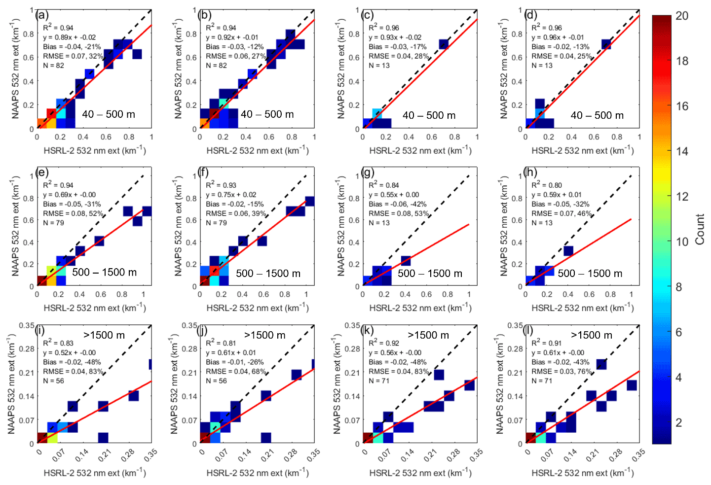
Figure 4 Comparison of simulated (NAAPS-RA) and retrieved (HSRL-2) 532 nm extinction coefficients when NAAPS-RA underestimated both extinction and RH. (a, b) Comparison when NAAPS-RA simulations were performed using either (a) NAAPS-RA RHs or (b) dropsonde RHs for altitudes between 40–500 m and when final dropsonde RHs are >80 %. (c, d) Same as (a, b, respectively) except when final dropsonde RHs were <80 %. (e, f) Same as (a, b, respectively) except for altitudes between 500–500 m. (g, h) Same as (e, f, respectively) except when final dropsonde RHs are <80 %. (i, j) Same as (a, b, respectively) except for altitudes >1500 m. (k, l) Same as (i, j) except when final dropsonde RHs are <80 %. Linear fits are indicated with red lines, 1:1 lines are shown as dotted lines, and the color bar shows the number of points falling in each bin. Where bias and RMSE are reported, the first and second numbers are the absolute and relative values, respectively.

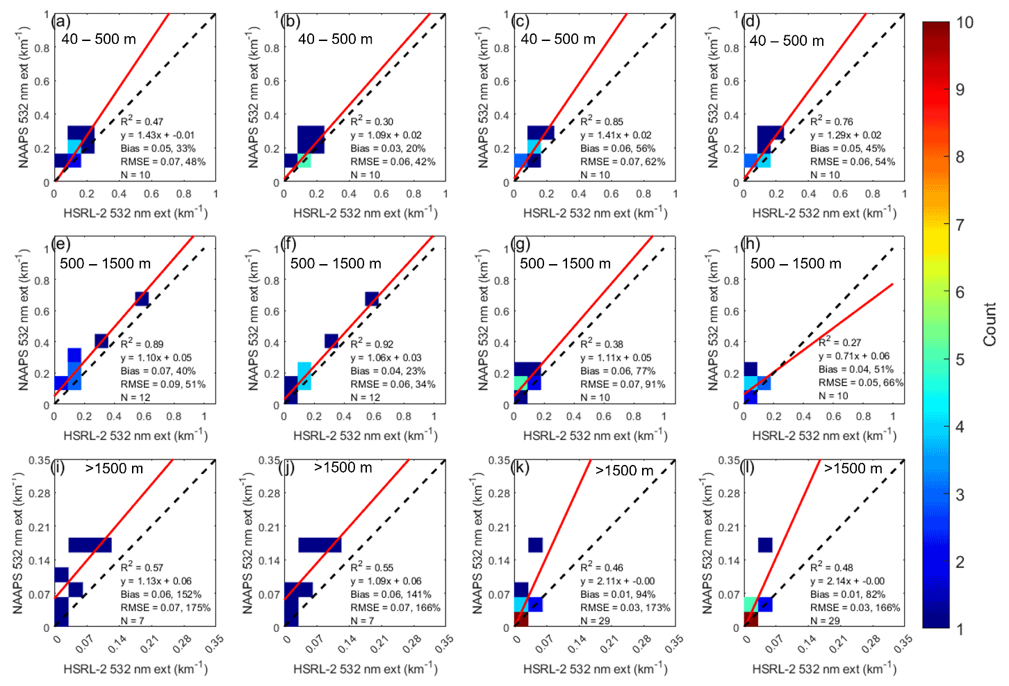
Figure 5 Same as Fig. 4 except when NAAPS-RA overestimated both extinction and RH. Linear fits are indicated with red lines, 1:1 lines are shown as dotted lines, and the color bar shows the number of points falling in each bin. Where bias and RMSE are reported, the first and second numbers are the absolute and relative values, respectively.

3.3 Investigating NAAPS-RA extinction sensitivity to changes in RH

We divided the extinction comparisons into six categories to understand (1) how opposing changes in extinction agreement within individual pressure layers may be negating changes in bulk statistics for the AOT and extinction comparison and (2) how sensitive changes in extinction are to the actual magnitude of the substituted dropsonde RH. Initial categorization isolated (i) pressure layers where NAAPS-RA both underestimated extinction and RH, (ii) pressure layers where NAAPS-RA both overestimated extinction and RH, and (iii) pressure layers where NAAPS-RA either underestimated extinction and overestimated RH or overestimated extinction and underestimated RH. Each of these three categories were divided again based on if the dropsonde RH for that pressure layer was greater than or less than 80 %.

NAAPS-RA extinction displays the best agreement with HSRL-2 retrievals (R², relative bias, and NRMSE values range from 0.80 %–0.96 %, −12 % to −48 % and 25 %–83 %, respectively; Fig. 4) in pressure layers where NAAPS-RA extinction and RH are both negatively biased. There are fewer pressure layers in which NAAPS-RA both overestimates extinction and RH because the model displays an overall negative bias for RH in all altitude layers. For these layers, there is poor to moderate agreement for some categories and relatively good agreement for others (R², relative bias, and NRMSE values range from 0.27 %–0.92 %, 20 %–152 %, and 34 %–175 %, respectively; Fig. 5). Over a quarter of the pressure layers in this category are from RF12, which sampled Asian pollution and smoke from biomass burning in Borneo advecting into the NWTP (average HSRL-2 AOTs ranged from 0.20±0.1–0.37±0.4 for the 1^∘ × 1^∘ grid cells considered from this flight). It is possible that NAAPS-RA is overestimating some aspect of the resulting air mass, whether it be particle hygroscopicity, particle mass concentrations, or a combination of the two. As discussed above, we do not have the data available to fully investigate this. When NAAPS-RA has opposing biases in extinction and RH, agreement is poor for some categories and relatively good for others (R², relative bias, and NRMSE values range from 0.41 %–0.96 %, −7 %–200 %, and 22 %–306 %; Fig. 6). Note that different sample sizes should be taken into consideration when comparing R² values between these categories (e.g., there is a relatively low number of points in the second category, i.e., pressure layers where NAAPS-RA overestimates both extinction and RH).

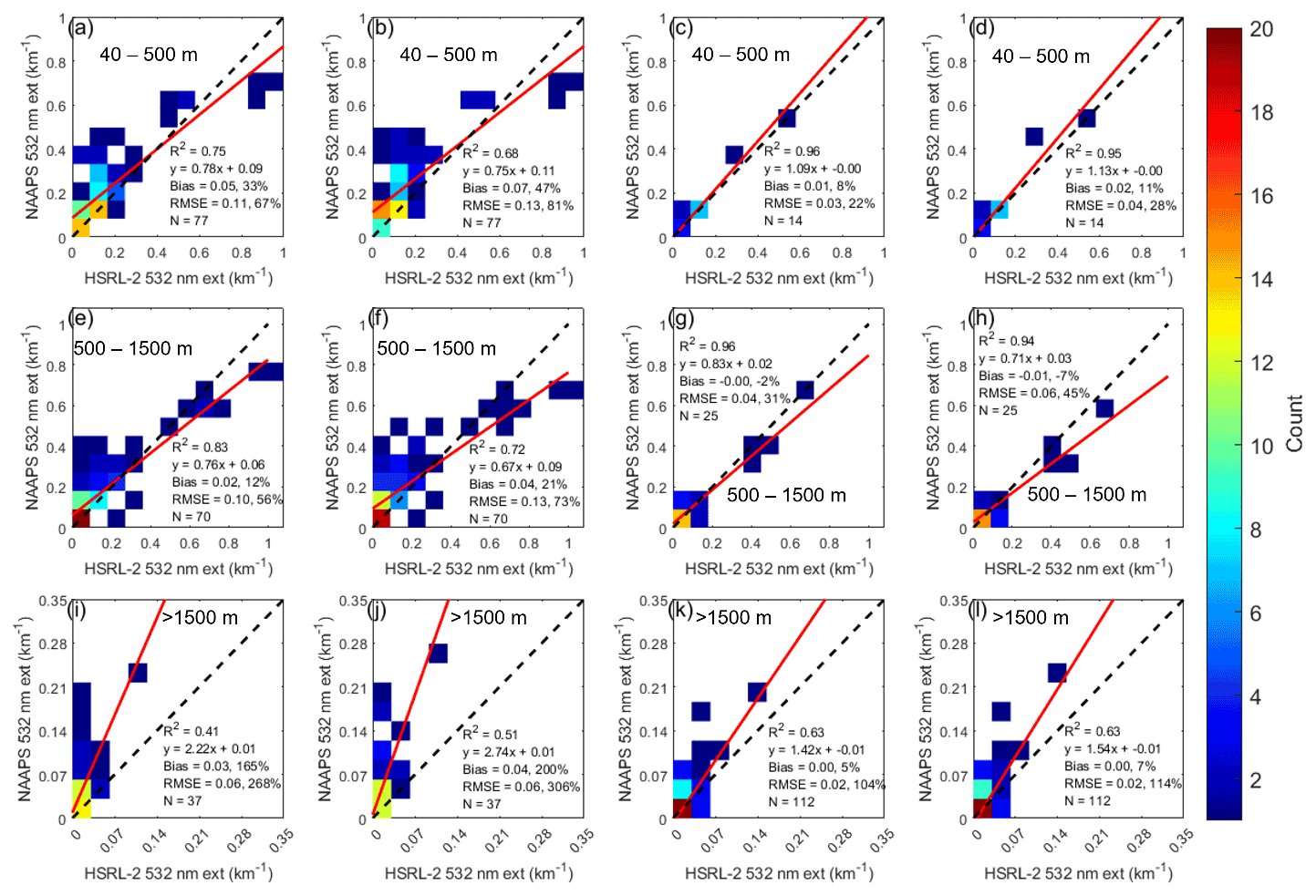
Figure 6 Same as Fig. 4 except when NAAPS-RA either (i) underestimated extinction and overestimated RH or (ii) overestimated extinction and underestimated RH. Linear fits are indicated with red lines, 1:1 lines are shown as dotted lines, and the color bar shows the number of points falling in each bin. Where bias and RMSE are reported, the first and second numbers are the absolute and relative values, respectively.

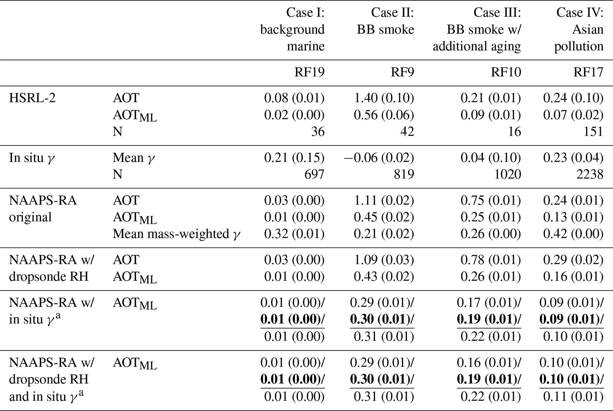
Table 3 Optical properties and summary statistics (means with standard deviations in parentheses) for NAAPS-RA/HSRL-2 comparisons for each case study. AOTML denotes AOT within the mixed layer (ML). Each case study is representative of a single $\mathrm{1}{}^{\circ }\times \mathrm{1}{}^{\circ }$ grid cell that was sampled during the flight indicated. “N” represents the number of data points. “BB” stands for biomass burning. The last two rows of the table report three sets of values where the first, second, and third sets are based on calculations using the γ value 1 standard deviation below the mean, the mean, and 1 standard deviation above the mean, respectively. Values calculated with the mean γ value are underlined and in bold font.

Most of the differences between simulated and retrieved values are between ∼ 0 and −0.05 km⁻¹ (Fig. S6) for pressure layers where NAAPS-RA underestimates extinction and RH, which may be why this category displays the best agreement. A larger fraction of differences falls above 0.05 km⁻¹ when NAAPS-RA overestimates extinction and RH (Fig. S7), and the distribution of differences is relatively wide when NAAPS-RA has opposing biases in extinction and RH (Fig. S8). This may explain why agreement is not as good for these latter two categories compared to the first category.

When dropsonde RHs are used, R² values do not improve for the first and second categories (pressure layers where NAAPS-RA either underestimates or overestimates both extinction and RH, respectively). However, shifts in bias and decreases in RMSE indicate that NAAPS-RA extinction coefficients are somewhat sensitive to corrections in RH. As expected, bias and RMSE increase for the third category (pressure layers where NAAPS-RA has opposing biases in extinction and RH) at all altitudes as substituting dropsonde RHs can only exacerbate the existing errors in simulated extinction for this category. Changes in absolute bias and RMSE are almost always detectable for altitudes below 1500 m and rarely detectable for altitudes above this, presumably because of the sharp decrease in magnitude for extinction coefficients above 1500 m.

Shifts in absolute bias and RMSE are greater for pressure layers with dropsonde RHs >80 % compared to layers with dropsonde RHs <80 %. Some of the largest differences between NAAPS-RA RH and dropsonde RH values (differences of 40 %–60 %) occur in pressure layers where dropsonde RHs are <80 % and the magnitude of the extinction coefficients ranges from 0.00–0.15 km⁻¹. However, when these dropsonde RHs are substituted, there is no overall change in absolute bias or RMSE. The fact that extinction agreement is almost entirely insensitive to this large of a shift in RH emphasizes the fact that changes in simulated extinction may be more sensitive to the actual magnitude of the final RH value and the magnitude of the extinction coefficients as opposed to the absolute error in RH. As mentioned above, NAAPS-RA extinction sensitivity to changes in RH also depends on speciated particle mass concentrations and/or the hygroscopicity assigned to each species. Sufficient data are not available to evaluate relationships between these parameters and extinction agreement between NAAPS-RA and HSRL-2 retrievals for the entire campaign. However, we confine our analysis to the ML (assumed to have homogeneous particle microphysical properties) for four case studies in the following section to provide some assessment of simulated hygroscopicity and particle mass concentrations.

3.4 Case studies

3.4.1 Case I: background marine (RF19)

RF19 sampled the cleanest conditions for the entire campaign and provided an opportunity to evaluate NAAPS-RA when AOT was very low (HSRL-2 AOT_ML and AOT ranged from 0.01–0.04 and 0.03–0.09, respectively, for the 1^∘ × 1^∘ grid cell considered for this flight). This period was associated with a mild tropical disturbance and advection of clean marine air from the northern subtropical western Pacific east of the Philippines (Hilario et al., 2021).

NAAPS-RA underestimates AOT_ML and AOT (MLH = 579 m; AOT_ML bias $=-\mathrm{0.01}$; AOT bias $=-\mathrm{0.05}$; Table 3) and underestimates extinction throughout the column (Fig. 7). Both the AOT_ML bias and shape of the NAAPS-RA extinction profile are largely unchanged when dropsonde RHs are used, which is unsurprising because vertically resolved model and dropsonde RHs are similar in the ML. A mean in situ γ value of 0.20 ± 0.16 indicates particles were less hygroscopic than has been observed for other clean marine environments ($\mathrm{0.38}\le \mathit{\gamma }\le \mathrm{0.73}$; Titos et al., 2016, and references therein). NAAPS-RA overestimates particle hygroscopicity, but correcting model γ values induces negligible changes in AOT_ML biases because extinction coefficients are already very low in magnitude for this case study. Slight increases in simulated particle mass concentrations and/or mass scattering and absorption efficiencies will likely allow NAAPS-RA to reach full agreement with the HSRL-2 extinction profile. NAAPS-RA appears to accurately simulate fine mass and overestimate coarse mass in our preliminary comparison of simulated and observed fine and coarse particle mass concentrations. However, we acknowledge there is great uncertainty in our method to derive coarse mass concentrations (as described in Sect. 2.6.3), especially considering ambient RHs do not fall below ∼ 80 % in the ML for this case study. We leave a more thorough closure analysis between simulated and observed mass concentrations to a future study.

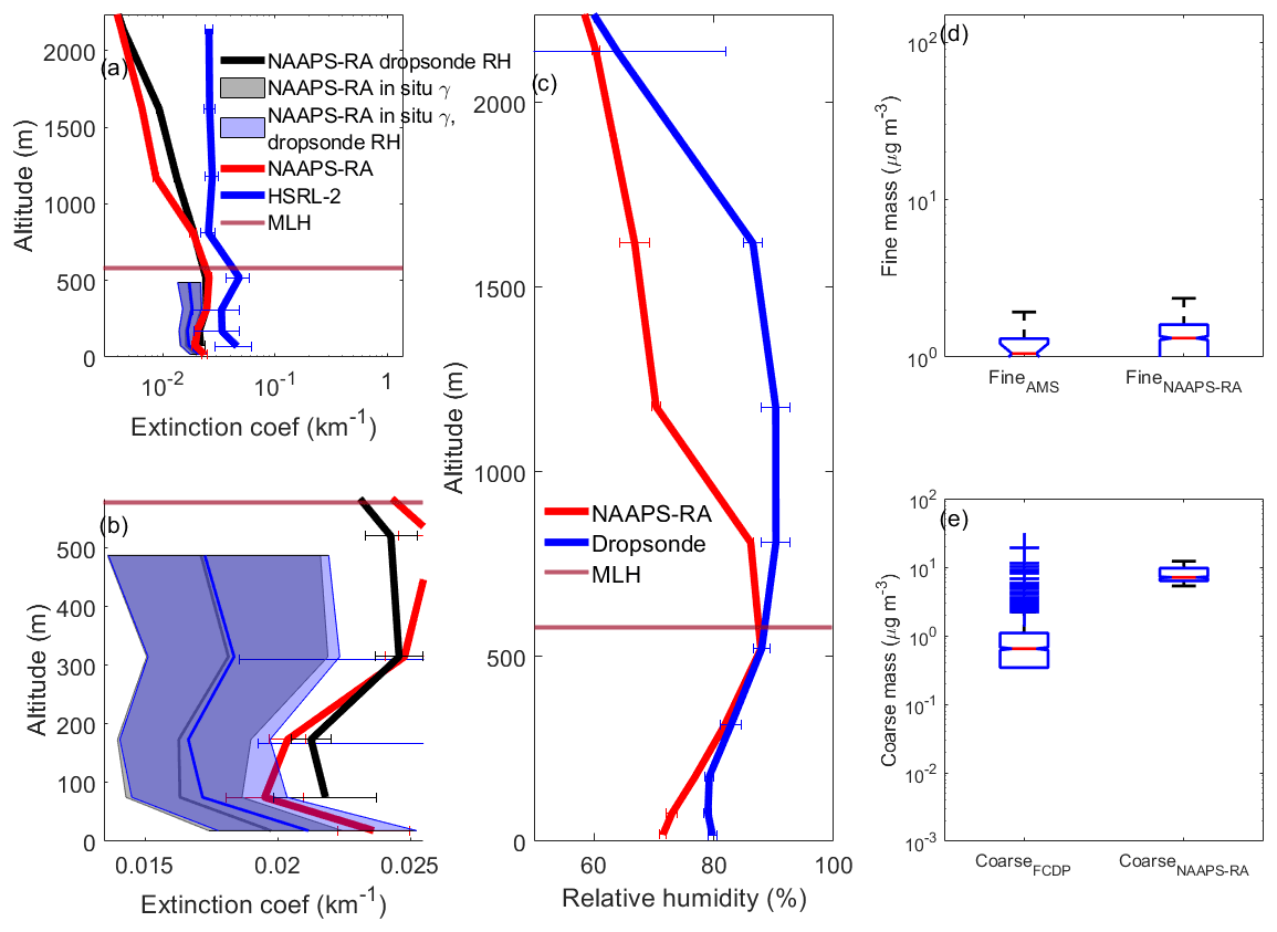
Figure 7 Comparison of model output and observations for Case I (RF19) on 5 October 2019. (a) HSRL-2 (blue) and NAAPS-RA extinction profiles when NAAPS-RA extinction coefficients were calculated using either NAAPS-RA RH (red) or dropsonde RH (black). Shaded profiles indicate NAAPS-RA extinction coefficients calculated using in situ γ values and either NAAPS-RA RH (grey shaded profile) or dropsonde RH (blue shaded profile). For each shaded profile, the middle line and lines bordering the right and left of each shaded profile indicate extinction coefficients calculated with either the mean γ, mean γ plus 1 standard deviation, or mean γ minus 1 standard deviation, respectively. (b) Shaded profiles shown in greater detail. (c) Dropsonde and NAAPS-RA RH profiles. Simulated and observed fine (d) and coarse (e) mass concentrations. The red line in the center of each box of (d) and (e) represents the median, the edges of each box indicate the 25 and 75th quartiles, blue crosses belong to outliers lying in the fourth quartile, and notches represent the 95 % confidence interval. Horizontal magenta lines in (a), (b), and (c) indicate the mixed-layer height (MLH; 579 m).

3.4.2 Case II: biomass burning smoke (RF9)

In contrast to the background marine case study, RF9 sampled the most polluted conditions for the campaign as smoke from the MC advected into the Sulu Sea (Hilario et al., 2021; HSRL-2 AOT_ML and AOT ranged from 0.45–0.68 and 1.26–1.58, respectively, for the 1^∘ × 1^∘ grid cell considered for this flight). Like the background marine case study, NAAPS-RA underestimates AOT_ML and AOT (MLH = 638 m; AOT_ML bias $=-\mathrm{0.11}$; AOT bias $=-\mathrm{0.29}$), but the model does capture the general shape of the extinction profile correctly in the ML (Fig. 8) so that the largest extinction coefficients are just below the MLH. Biases become more negative when dropsonde RHs are used (AOT_ML bias $=-\mathrm{0.13}$; AOT bias $=-\mathrm{0.31}$) because NAAPS-RA underestimates RH at altitudes up to ∼ 250 m and overestimates RH from ∼ 250 to the MLH. The decrease in modeled RH to measured RH at altitudes where extinction coefficients are highest causes the recalculated NAAPS-RA extinction profile to fall even further behind the HSRL-2 profile at these same altitudes, and agreement worsens.

Figure 8 Same as Fig. 7 except for Case II (RF9) on 15 September 2019. The MLH is 638 m.

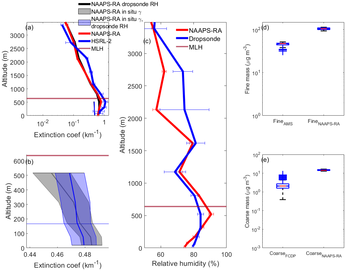
The observation of negative γ values in smoke plumes advecting towards the Philippines from the southwest is arguably one of the more interesting preliminary results from the CAMP²Ex field campaign. However, errors in these observations may still exist given the nature of the particle chemistry. Nevertheless, f(RH) was low, and negative in situ γ values (−0.06 ± 0.02) observed on this flight may imply that a majority of the smoke particles were nonspherical and collapsed into spherical morphology upon humidification (Shingler et al., 2016). In contrast, NAAPS-RA assigns a slightly positive γ value to smoke particles based on a global average. Thus, when in situ γ values are used, biases in AOT_ML become even larger (from −0.25 to −0.27), and the HSRL-2 extinction profile cannot even be seen in the frame of Fig. 8b. This implies NAAPS-RA is underestimating either fine mass, coarse mass, or scattering and absorption efficiencies (or some combination of these parameters). Our preliminary assessment of simulated versus observed fine and coarse particle mass concentrations suggests that NAAPS-RA is overestimating both fine and coarse mass, but we report this result with caution. The large discrepancies in extinction between NAAPS-RA and HSRL-2 retrievals are likely due in some part to errors in simulated particle mass concentrations, and we encourage future work to investigate this more deeply.

3.4.3 Case III: biomass burning smoke with additional aging (RF10)

RFs 9 and 10 were coordinated such that biomass burning emissions from the MC were sampled on subsequent days, which provided an opportunity to learn how smoke particle composition and hygroscopicity (among other air mass properties) changed with ∼ 24 h of additional aging. Aged smoke was the dominant air mass in the ML for the 1^∘ × 1^∘ grid cell selected for this case study, but conditions were considerably less polluted compared to RF9 (MLH = 593 m; HSRL-2 AOT_ML and AOT ranged from 0.08–0.11 and 0.20–0.23, respectively, for the grid cell considered in this case study).

AMS data indicate the smoke plume sampled during RF9 and RF10 had very similar chemical composition (Fig. S9), yet in situ γ values for RF10 suggest the air mass entering the Philippine Sea was more hygroscopic (γ= 0.04 ± 0.10) than the air mass sampled in the Sulu Sea during RF9 ($\mathit{\gamma }=-\mathrm{0.06}\pm \mathrm{0.02}$). However, the hygroscopic properties of this smoke mass are not straightforward as both positive and negative γ values were observed. More work is needed to fully explain this phenomenon. Nonetheless, NAAPS-RA treats all smoke particles the same, no matter their age, motivating interest in how such an assumption could lead to errors in simulated extinction.

For this case study, NAAPS-RA greatly overestimates AOT_ML and AOT (biases of 0.16 and 0.54 respectively; Fig. 9). NAAPS-RA slightly underestimates RH throughout the ML (and up to ∼ 2100 m), so agreement only worsens when dropsonde RHs are substituted into the model (AOT_ML and AOT bias = 0.17 and 0.57, respectively).

Figure 9 Same as Fig. 7 except for Case III (RF10) on 16 September 2019. The MLH is 593 m.

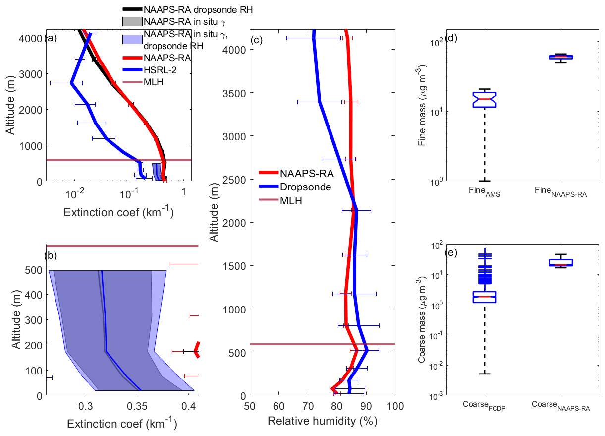
Similar to Case II, the model overestimates the hygroscopicity of smoke particles in this air mass (mean in situ and simulated γ values are 0.04±0.10 and 0.26±0.00, respectively). After adopting in situ RHs and γ values, NAAPS-RA overestimates AOT_ML (biases range from 0.07–0.13), suggesting there is likely a positive bias for fine and/or coarse particle mass concentrations and/or mass scattering and absorption efficiencies. NAAPS-RA appears to overestimate both fine and coarse particle mass concentrations in the ML, but additional work is needed to study agreement between in situ and simulated particle mass concentrations.

3.4.4 Case IV: Asian pollution (RF17)

This case study provides an opportunity to assess NAAPS-RA performance for an air mass dominated by urban pollution from East Asia with moderate AOT (HSRL-2 AOT_ML and AOT ranged from 0.03–0.14 and 0.13–0.41, respectively). The model overestimates extinction (AOT_ML bias = 0.06; Fig. 10) and underestimates RH for all pressure layers within the ML (MLH = 535 m). When dropsonde RHs are substituted into the model, AOT_ML bias increases to 0.09, and extinction increases drastically in the pressure layer where dropsonde RH exceeds 90 %. NAAPS-RA simulates ABF as the dominant species in this air mass (average mass fraction of 0.70±0.01), which the model considers as the most hygroscopic aerosol type. The prevalence of this species in combination with relatively high dropsonde RHs within the ML makes the large increase in AOT_ML expected.

Figure 10 Same as Fig. 7 except for Case IV (RF17) on 1 October 2019. The MLH is 535 m.

ABF is arguably one of the most difficult aerosol types for NAAPS-RA to accurately model as it combines organic and inorganic species, which can have very different hygroscopic and optical properties. NAAPS-RA assigns a γ value to ABF by assuming 40 % SO${}_{\mathrm{4}}^{\mathrm{2}-}$ and 60 % OA. However, the composition of anthropogenic and biogenic emissions is likely to vary across different regions. For example, mean fine mass fractions of SO${}_{\mathrm{4}}^{\mathrm{2}-}$ and OA (0.62±0.04 and 0.22±0.03, respectively) for this case study are largely different from what the model assumes, motivating interest in how AOT_ML will adjust when observed γ values are substituted into the model. The mean in situ γ value (0.23±0.04) is nearly half the mean NAAPS-RA mass-weighted γ (0.42±0.00) and the γ value assigned to ABF (0.46). When in situ γ values are used in the model, extinction agreement improves dramatically (AOT_ML biases drop to a range of 0.02–0.03), which suggests that the γ value assigned to ABF requires modification for this region.

Even with corrected RHs and γ values, NAAPS-RA overestimates AOT_ML for this 1^∘ × 1^∘ grid cell, which implies the model is overestimating fine and/or coarse particle mass concentrations and/or scattering and absorption efficiencies. Our preliminary comparison of simulated and observed fine and coarse mass concentrations indicates simulated mass concentrations are too high, but as we have mentioned, more work must be done before we can comment on these mass concentrations with certainty.

4 Conclusions

This study evaluates NAAPS-RA AOT and extinction outputs during the CAMP²Ex field campaign. Simulations of AOT and extinction are compared to collocated retrievals made with a HSRL-2 over the course of 19 research flights. Extinction coefficients are evaluated in three altitude layers (40–500, 500–1500 m, and above 1500 m) to evaluate model performance within the mixed layer (ML), in the transition from the ML to the free troposphere (FT), and in the FT, respectively. Profiles of relative humidity (RH) measured with dropsondes are substituted into the model to explore how correcting errors in modeled RH affects simulations for AOT and extinction. Additionally, four case studies are analyzed within the ML to investigate how simulations of extinction change when in situ observations of the hygroscopic growth parameter, γ, and RH are substituted into the model. The main findings of this work are as follows:

• NAAPS-RA shows relatively good agreement with HSRL-2 retrievals for AOT (R²= 0.78; NRMSE = 48 %) and extinction (R²= 0.80, 0.81, and 0.42; NRMSE = 47 %, 53 %, and 118 % for altitudes of 40–500 m, 500–1500 m, and >1500 m, respectively) considering that there were few instances of AOT assimilations from MODIS and MISR over the course of the campaign.

• NAAPS-RA shows poor RH correlation with dropsonde measurements and underestimates RH in each altitude layer (R²= 0.16, 0.19, and 0.48; absolute biases $=-\mathrm{5}$ %, −8 %, and −3 % for altitudes of 0–500, 500–1500 m, and >1500 m, respectively).

• AOT and extinction agreement does not improve (R²= 0.77; NRMSE = 49 % (AOT) and R²= 0.78, 0.78, and 0.46; NRMSE = 51 %, 56 %, and 117 % (for extinction within altitudes of 40–500, 500–1500 m, and >1500 m, respectively)) when dropsonde RHs are substituted into the model despite considerable differences between simulated and measured RH. However, biases in model AOT and extinction at all altitudes shift in a positive direction, which indicates that fixing errors in modeled RH has some effect on model outputs for AOT and extinction.

• Changes in simulated extinction are more sensitive to the actual magnitude of the extinction coefficients and magnitude of the dropsonde RHs substituted into the model rather than the absolute differences between the model and dropsonde RHs.

• The model overestimates γ for (i) aged smoke particles transported from the MC and (ii) anthropogenic and biogenic fine (ABF) particles in an air mass dominated by East Asian outflow.

Figure 12 in Lynch et al. (2016) shows that R² values for comparisons between simulated (NAAPS-RA) and retrieved (AERONET) AOT values from around the world are slightly lower than our values for this study. Although we can see AOT agreement does not fluctuate too much across the globe, the driving forces behind disagreement in these locations are presumably uncertain. However, it is likely that the model's simple representation of speciated particle composition, hygroscopicity, and size contributes to these errors in some part. Findings from this work can assist members of the modeling community to begin understanding sources of error in modeled AOT so that forecasts can be improved in SEA and beyond. For example, our results reveal NAAPS-RA overestimates the hygroscopicity of particles from biomass burning in the MC as well as anthropogenic particles transported from East Asia, which leads to inaccurate extinction outputs. This result may apply to other smoke plumes and/or urban environments, motivating future works to examine model performance in these types of air masses elsewhere.