the Creative Commons Attribution 4.0 License.
the Creative Commons Attribution 4.0 License.
 | 26 Sep 2022
Multi-axis differential optical absorption spectroscopy (MAX-DOAS) observations of formaldehyde and nitrogen dioxide at three sites in Asia and comparison with the global chemistry transport model CHASER
Hossain Mohammed Syedul Hoque
Kengo Sudo
Hitoshi Irie
Alessandro Damiani
Manish Naja
Al Mashroor Fatmi
Formaldehyde (HCHO) and nitrogen dioxide (NO2) concentrations and profiles were retrieved from ground-based multi-axis differential optical absorption spectroscopy (MAX-DOAS) observations during January 2017–December 2018 at three sites in Asia: (1) Phimai (15.18∘ N, 102.5∘ E), Thailand; (2) Pantnagar (29∘ N, 78.90∘ E) in the Indo-Gangetic Plain (IGP), India; and (3) Chiba (35.62∘ N, 140.10∘ E), Japan. Retrievals were performed using the Japanese MAX-DOAS profile retrieval algorithm ver. 2 (JM2). The observations were used to evaluate the NO2 and HCHO partial columns and profiles (0–4 km) simulated using the global chemistry transport model (CTM) CHASER (Chemical Atmospheric General Circulation Model for Study of Atmospheric Environment and Radiative Forcing). The NO2 and HCHO concentrations at all three sites showed consistent seasonal variation throughout the investigated period. Biomass burning affected the HCHO and NO2 variations at Phimai during the dry season and at Pantnagar during spring (March–May) and post-monsoon (September–November). Results found for the HCHO-to-NO2 ratio (RFN), an indicator of high ozone sensitivity, indicate that the transition region (i.e., 1 < RFN < 2) changes regionally, echoing the recent finding for RFN effectiveness. Moreover, reasonable estimates of transition regions can be derived, accounting for the NO2–HCHO chemical feedback.
The model was evaluated against global NO2 and HCHO columns data retrieved from Ozone Monitoring Instrument (OMI) observations before comparison with ground-based datasets. Despite underestimation, the model well simulated the satellite-observed global spatial distribution of NO2 and HCHO, with respective spatial correlations (r) of 0.73 and 0.74. CHASER demonstrated good performance, reproducing the MAX-DOAS-retrieved HCHO and NO2 abundances at Phimai, mainly above 500 m from the surface. Model results agree with the measured variations within the 1-sigma (1σ) standard deviation of the observations. Simulations at higher resolution improved the modeled NO2 estimates for Chiba, reducing the mean bias error (MBE) for the 0–2 km height by 35 %, but resolution-based improvements were limited to surface layers. Sensitivity studies show that at Phimai, pyrogenic emissions contribute up to 50 % and 35 % to HCHO and NO2 concentrations, respectively.
- Article
(3567 KB) - Full-text XML
-
Supplement
(1386 KB) - BibTeX
- EndNote


Formaldehyde (HCHO), the most abundant carbonyl compound in the atmosphere, is a high-yield product of oxidization of all primary volatile organic compounds (VOCs) emitted from natural and anthropogenic sources by hydroxyl radicals (OH). Oxidation of long-lived VOCs such as methane produces a global HCHO background concentration of 0.2–1.0 ppbv in remote marine environments (Weller et al., 2000; Burkert et al., 2001; Singh et al., 2004; Sinreich et al., 2005). Aside from oxidation of VOCs, the significant sources of HCHO are direct emissions from biomass burning, industrial processes, fossil fuel combustion (Lee et al., 1997; Hak et al., 2005; Fu et al., 2008), and vegetation (Seco et al., 2007). However, oxidization of non-methane VOCs emitted from biogenic (e.g., isoprene) or anthropogenic (e.g., butene) sources governs the spatial variation in HCHO on a global scale (Franco et al., 2015). The sinks of HCHO include photolysis at wavelengths shorter than 400 nm, oxidation by OH, and wet deposition, thereby limiting the lifetime of HCHO to a few hours (Arlander et al., 1995).
Nitrogen dioxide (NO2), an important atmospheric constituent, (1) participates in the catalytic formation of tropospheric ozone (O3), (2) acts as a catalyst for stratospheric ozone (O3) destruction (Crutzen, 1970), (3) contributes to the formation of aerosols (Jang and Kamens, 2001), (4) acts as a precursor of acid rain (Seinfeld and Pandis, 1998), and (5) strongly affects radiative forcing (Solomon et al., 1999; Lelieved et al., 2002). Nitrogen oxides (NOx = NO (nitric oxide) + NO2) are emitted from natural and anthropogenic sources. Primary NOx emission sources include biomass burning, fossil fuel combustion, soil emissions, and lightning (Bond et al., 2001; Zhang et al., 2003). Not only do NOx emissions degrade air quality, but they are also leading air pollutants (Ma et al., 2013). Both HCHO and NO2 are important intermediates in the global VOC–HOx (hydrogen oxides)–NOx catalytic cycle, which governs O3 chemistry in the troposphere (Lee et al., 1997; Houweling et al., 1998; Hak et al., 2005; Kanakidou et al., 2005). Thus, both trace gases play crucially important roles in tropospheric chemistry.
The observational sites examined for the present study have different atmospheric characteristics. Thailand is strongly affected by pollution because of rapid economic development and urbanization. Moreover, biomass burning in Southeast Asia is a significant source of O3 precursors, contributing up to 30 % of the total concentrations during the peak burning season (Amnuaylorajen et al., 2020; Khodmanee and Amnuaylojaroen, 2021). Because of rapid industrialization, India, the second-most populous country in the world, is witnessing an increasing O3 trend along with increasing NO2 and HCHO concentrations in all major cities (Mahajan et al., 2015; Lu et al., 2018). The Indo-Gangetic Plain (IGP), which covers ∼ 21 % of the Indian subcontinent land area, has hotspots of severe air pollution (Giles et al., 2011; Biswas et al., 2019). In contrast, surface O3 concentrations have shown an increasing trend in Japan, despite decreasing NOx and VOC concentrations related to emission control measures after 2000 (Irie et al., 2021). Therefore, observational and modeling studies must be conducted to improve our quantitative understanding of the O3–NOx–VOC relation in these regions.
Multi-axis differential optical absorption spectroscopy (MAX-DOAS), a well-established, unique, and powerful remote sensing method for measuring trace gases and aerosols, is based on the DOAS technique. Aerosols and trace gases are quantified using selective narrowband (high-frequency) absorption features (Platt and Stutz, 2008). Spectral radiance measurements at different elevation angles (ELs) can provide profile information about atmospheric trace gases and aerosols (Hönninger et al., 2004; Wagner et al., 2004; Wittrock et al., 2004; Frieß et al., 2006; Irie et al., 2008a). Many studies have demonstrated the retrieval of aerosol and trace gas concentrations and profiles, including NO2 and HCHO, from MAX-DOAS observations (Clémer et al., 2010; Irie et al., 2011; Hendrick et al., 2014; Wang et al., 2014; Franco et al., 2015; Frieß et al., 2016).
The ability of MAX-DOAS to provide information related to surface concentrations, vertical profiles, and column densities makes it a good complement to ground-based in situ and satellite observations. Moreover, the MAX-DOAS method uses narrowband absorption of the target compounds, thereby obviating any need for radiometric calibration of the instrument. Because of these advantages, MAX-DOAS systems are deployed for the assessment of aerosol and trace gases in regional and global observational networks such as BREDOM (Wittrock et al., 2004), BIRA-IASB (Clémer et al., 2010), and MADRAS (Kanaya et al., 2014). Such datasets are used in, but are not limited to, (1) air quality assessment and monitoring, (2) evaluation of chemistry transport models (CTMS), and (3) validation of satellite data retrievals. Several studies have used MAX-DOAS datasets to validate tropospheric columns retrieved from satellite observations, including NO2 and HCHO (Irie et al., 2008b; Ma et al., 2013; Chan et al., 2020; Ryan et al., 2020). However, limited MAX-DOAS datasets have been used to evaluate global CTMs. Vigouroux et al. (2009) and Franco et al. (2015) used the MAX-DOAS HCHO datasets from the island of Réunion and Jungfraujoch stations, respectively, to evaluate the Intermediate Model of Annual and Global Evolution of Species (IMAGES) and GEOS-Chem model simulations. Kanaya et al. (2014) validated the Model for Interdisciplinary Research on Climate Earth system model with chemistry (MIROC-ESM-CHEM)-simulated NO2 column densities with MAX-DOAS observations in Cape Hedo and Fukue in Japan. Kumar and Sinha (2021) used MAX-DOAS observations to evaluate the high-resolution regional model MECO(n) (MESSy-fied ECHAM and COSMO models nested n times).
For this study, NO2 and HCHO profiles retrieved from MAX-DOAS observations from the international air quality and sky research remote sensing (A-SKY; Irie, 2021) network sites are used to evaluate the global Chemical Atmospheric General Circulation Model for Study of Atmospheric Environment and Radiative Forcing (CHASER; Sudo et al., 2002). The three A-SKY sites of (1) Phimai in Thailand (15.18∘ N, 102.56∘ E), (2) Pantnagar (29∘ N, 78.90∘ E) in the IGP in India, and (3) Chiba (35.62∘ N, 140.10∘ E) in Japan are representative of rural, semi-rural, and urban environments, respectively. CHASER has been used mostly for global-scale research (Sudo and Akimoto, 2007; Sekiya and Sudo, 2014; Sekiya et al., 2018; Miyazaki et al., 2017). The study described herein is the first reported attempt to evaluate the CHASER-simulated NO2 and HCHO profiles using MAX-DOAS observations in three different atmospheric environments. Moreover, few reports of the literature have described the use of MAX-DOAS datasets to evaluate global CTMs in South Asia and Southeast Asia. Overall, this study was conducted to provide important insights into model performance and to help reduce model uncertainties related to NO2 and HCHO simulations in these regions.
The paper is structured in the following manner. First, the observation sites, MAX-DOAS instrumentation, and retrieval strategies are described in Sect. 2. Section 2 also includes a short description of the CHASER model and Ozone Monitoring Instrument (OMI) HCHO and NO2 retrievals. Next, the observations and the evaluation results are described in Sect. 3. Finally, the sensitivity study results are provided in Sect. 3.4. and the concluding remarks in Sect. 4.
2.1 Site information
Continuous MAX-DOAS observations at Chiba, Phimai, and Pantnagar started in 2012, 2014, and 2017, respectively. The measurements from January 2017 to December 2018 at all three sites are discussed herein. Phimai, a rural site, is located ∼ 260 km northeast of the Bangkok metropolitan area and is unlikely to be affected by vehicular and industrial emissions. However, the site is affected by biomass burning during January–April. Two major air streams, the dry, cool northeast monsoon during November–mid-February and the wet, warm southwest monsoon during mid-May–September, affect the climate in Phimai. As described by Hoque et al. (2018a), the climate classifications of Phimai are the (a) dry season (January–April) and (b) wet season (June–September).
Pantnagar, a semi-urban site in India, is located in the IGP. The Indian capital of New Delhi is situated ∼ 225 km southwest of the site. The low-altitude plains are on the south and west sides of the site. The Himalayan mountains are located to the north and east. An important roadway with a moderate traffic volume and a small local airport lies within 3 km of the site. Rudrapur (∼ 12 km southwest of Pantnagar) and Haldwani (∼ 25 km northeast of Pantnagar) are the two major cities near Pantnagar, where non-combustible industries are located (Joshi et al., 2016). The climate classification at Pantnagar is the following: (1) winter (December–February), (2) spring (March–May), (3) summer monsoon (June–August), and (4) autumn (September–November).

Figure 1Surface HCHO mixing ratio in June 2018, simulated using the CHASER model. The red points represent the locations of the observation sites, which are part of the A-SKY network.
Chiba, an urban site, is located ∼ 40 km southeast of the Tokyo metropolitan region. Tokyo Bay, large-scale industries, and residential areas are located within a 50 km radius. Chiba has four distinct seasons: (1) spring (March–May), (2) summer (June–August), (3) autumn (September–November), and winter (December–February). The locations of the three sites are depicted in Fig. 1.
2.2 MAX-DOAS retrieval
The MAX-DOAS systems used for continuous observations at the three sites participated in the Cabauw Intercomparison campaign for Nitrogen Dioxide measuring Instruments (CINDI) (Roscoe et al., 2010) and CINDI-2 (Kreher et al., 2020) campaigns. The instrumentation setup is described by Irie et al. (2008a, 2011, 2015). The indoor part of the MAX-DOAS systems consists of an ultraviolet–visible (UV–VIS) spectrometer (Maya2000 Pro; Ocean Optics, Inc.) embedded in a temperature-controlled box. The outdoor unit consists of a single telescope and a 45∘ inclined movable mirror on a rotary actuator, used to perform reference and off-axis measurements. The high-resolution spectra from 310–515 nm is recorded at six elevation angles (ELs) of 2, 3, 4, 6, 8, and 70∘ at the Chiba and Phimai sites. At the Pantnagar site, measurements are conducted at ELs of 3, 4, 5, 6, 8, and 70∘. The sequences of the ELs at all the sites are repeated every 15 min. The reference spectra are recorded at EL of 70∘ instead of 90∘ to avoid saturation of intensity. Because all the ELs were considered in the box air mass factor (Abox) calculation to retrieve the vertical profile, the choice of reference EL (70∘ or 90∘) is not an important issue for this study. The off-axis ELs are limited to < 10∘ to reduce the systematic error in the in-oxygen collision complex (O4) fitting results (Irie et al., 2015), thereby maintaining high sensitivity in the lowest layer of the retrieved aerosol and trace gas profiles. Daily wavelength calibration using the high-resolution solar spectrum from Kurucz et al. (1984) is performed to account for the spectrometer's long-term degradation. The spectral resolution (full width half maximum, FWHM) is about 0.4 nm at 357 and 476 nm. The concentrations and profiles of aerosol and trace gases are retrieved using the Japanese vertical profile retrieval algorithm (JM2 ver. 2) (Irie et al., 2011, 2015). The algorithm works in three steps: (1) DOAS fittings, (2) profile and column retrieval of aerosol, and (3) profile and column retrieval of trace gases. Irie et al. (2008a, b, 2011, 2015) described the retrieval procedures and the error estimates. Herein we provide a short overview.
Table 1Cross-section data references and absorbers fitted in the HCHO and NO2 windows.
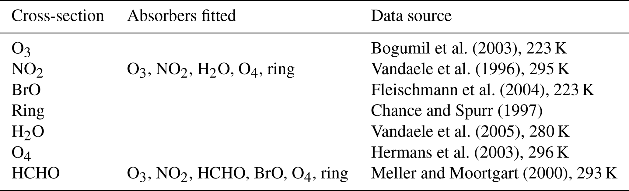

Figure 2Examples of spectral fitting of NO2 and HCHO, where red and black lines show the scaled cross-section and the summation of scaled cross-sections and fitting residuals, respectively. The example shows the measurements of 10 April 2017, in Phimai at 10:00 LT at an EL of 2∘.
First, the differential slant column density (ΔSCD) of trace gases is retrieved using the DOAS technique (Platt and Stutz, 2008), which uses the non-linear least-squares spectral fitting method, according to the following equation:
Therein, Io(λ) represents the reference spectrum measured at time t. Io(λ) is derived by interpolating two reference spectra (i.e., EL = 70∘) within 15 min before and after the complete sequential scan of the off-axis ELs at time t. ΔSCD represents the difference between the slant column density along the off-axis and reference spectrum. Second- and third-order polynomials are fitted to account for the wavelength-dependent offset c(λ) and the effect of molecular and particle scattering p(λ), respectively. In addition, c(λ) accounts for the influence of stray light. The HCHO ΔSCD and NO2 ΔSCD are retrieved from the fitting windows of 340–370 and 460–490 nm, respectively. Significant O4 absorptions in the 338–370 and 460–490 nm fitting windows are used to retrieve the O4 ΔSCDs. The absorption cross-section data sources and the fitted absorbers in the HCHO and NO2 fitting windows are given in Table 1. Figure 2 presents an example of the fitting results. O4 fittings in both retrieval windows are shown in Fig. S1 (Supplement).
In the second step, the aerosol optical depth (AOD) τ and the vertical profiles of the aerosol extinction coefficient (AEC) k are retrieved using the approach developed by Irie et al. (2008a), which is based on the optimal estimation method (Rodgers, 2000). In this approach, the measurement vector y (representing the quantities to be fitted) and state vector (representing the retrieved quantities) are defined as
and
where n stands for the number of measurements within one complete scan of an EL sequence. Also, Ω denotes the viewing geometry and includes three components: the solar zenith angle (SZA), EL, and relative azimuth angle (RAA). The F values determine the profile shape, with values between 0 and 1. The partial AOD for 0–1, 1–2, 2–3, and above 3 km layers was defined as AOD × F1, AOD × (1−F1)F2, AOD × , and AOD × , respectively. The AEC profile from 3 to 100 km is derived assuming a fixed value at 100 km and exponential AEC profile shape with a scaling height of ∼ 1.6 km. The k value at 100 km was estimated from Stratospheric Aerosol and Gas Experiment III (SAGE III) aerosol data (λ = 448 and 521 nm) taken at altitudes of 15–40 km. The negligible influence of such assumptions on the retrievals in the lower troposphere has been demonstrated in sensitivity studies reported by Irie et al. (2009). Similarly, the AEC profiles at 2–3, 1–2, and 0–1 km were derived. Such parameterization provides the advantage that the AEC profile can be retrieved using only the a priori knowledge of the F values (profile shape) and little or no information related to the absolute AEC values in the troposphere. Irie et al. (2008a) demonstrated that the relative variability in the profile shape, in terms of 1 km averages, is smaller than that of the absolute AEC values. AEC profile shapes corresponding to different F values are shown in Fig. S2 (Supplement). However, the vertical resolution and the measurement sensitivity cannot be derived directly with such a parameterization (Irie et al., 2008a, 2009). The retrievals and simulations conducted by other groups for similar geometries (i.e., Frieß et al., 2006) are used to overcome such limitations. The a priori values used for this study were similar to those reported by Irie et al. (2011): AOD = 0.21 ± 3.0, F1 = 0.60 ± 0.05, F2 = 0.80 ± 0.03, and F3 = 0.80 ± 0.03.
Then, a lookup table (LUT) of the box air mass factor (Abox) vertical profile at 357 and 476 nm is constructed using the radiative transfer model JACOSPAR (Irie et al., 2015), which is based on the Monte Carlo Atmospheric Radiative Transfer Simulator (MCARaTS) (Iwabuchi, 2006). The values of the single-scattering albedo (s), asymmetry parameter (g), and surface albedo were 0.95, 0.65 (under the Henyey–Greenstein approximation), and 0.10, respectively. The US standard atmosphere temperature and pressure profiles were used for radiative transfer calculations. Uncertainty of less than 8 % related to the usage of fixed values of s, g, and a was estimated from sensitivity studies (i.e., Irie et al., 2009). Results obtained from JACOSPAR are validated in the study reported by Wagner et al. (2007). The optimal aerosol load and the Abox profiles are derived using the Abox LUT and the O4 ΔSCD at all ELs.
In the third step, the Abox profiles, HCHO and NO2 ΔSCDs, and the non-linear iterative inversion method are used to retrieve the HCHO and NO2 vertical column densities (VCDs) and profiles. Here the NO2 retrieval is explained.
For trace gas retrieval, the measurement vector and state vector are defined as
and
VCD represents the vertical column density below 5 km. The f values are the profile shape factors. Above the 5 km layer, fixed profiles are assumed. Similarly to aerosol retrieval, the partial VCD values for 0–1, 1–2, 2–3, and 3–5 km are defined as VCD × f1, VCD × (1−f1)f2, VCD × , and VCD × , respectively. Finally, the volume mixing ratio (VMR) is calculated using the partial VCD and US standard atmosphere temperature and pressure data scaled to the respective surface measurements.
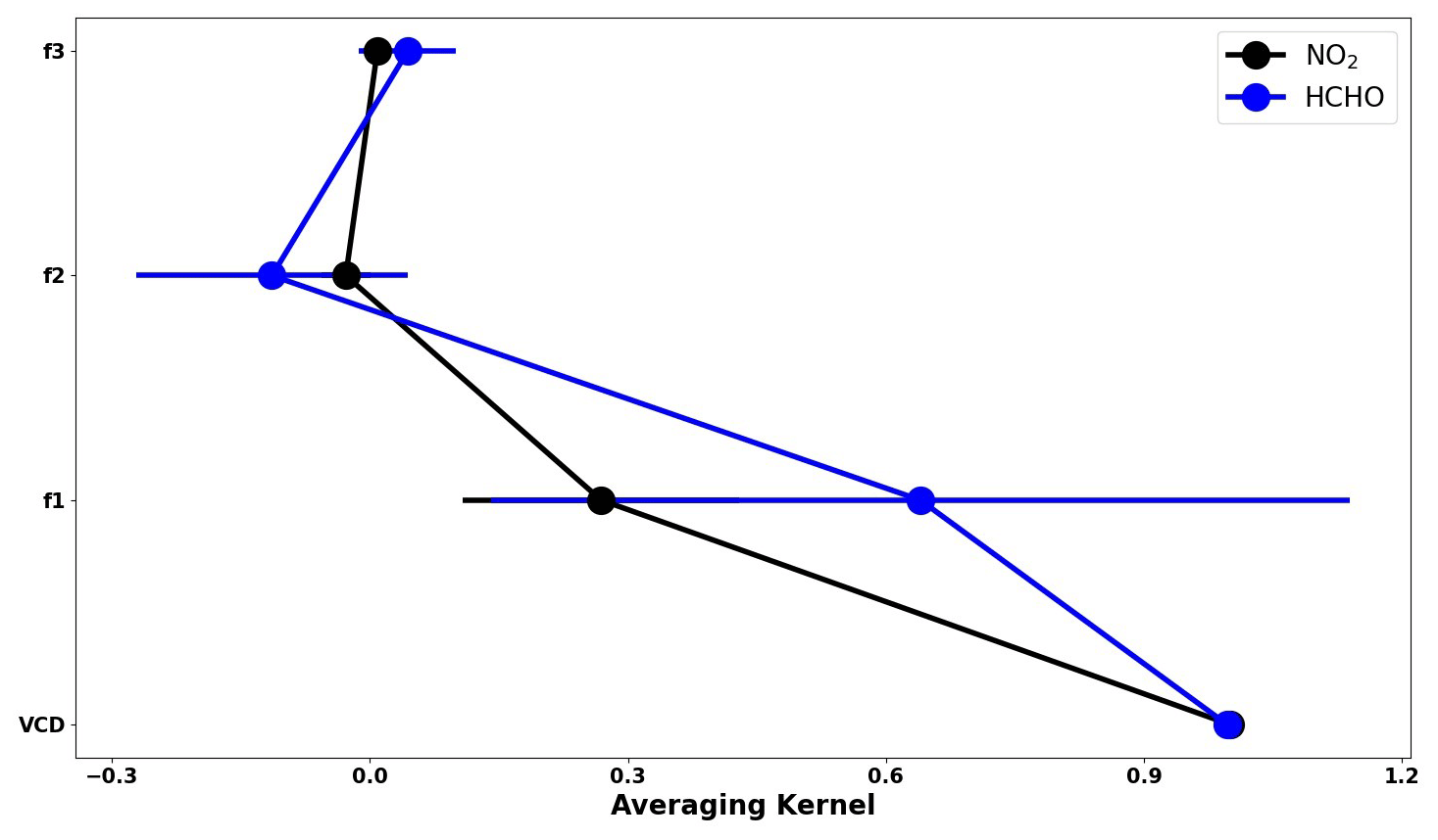
Figure 3Mean averaging kernel of the NO2 and HCHO retrievals from observations at Phimai during 2017. The error bars represent the 1σ standard deviation of the mean values.
The calculated vertical profile is converted to NO2 ΔSCDs using the Abox LUT constructed for aerosol retrieval. However, the trace gas wavelengths differed from the representative wavelengths of the Abox LUT (357 and 476 nm). Therefore, the AOD at the trace gas wavelength is estimated, converting the retrieved AOD to the closer aerosol wavelength of 357 or 476 nm, assuming an Ångström exponent value of 1.00. The choice of the Ångström exponent value can induce uncertainty in the retrieved VCDs. However, such uncertainty was found to be non-significant compared to that of Abox profiles. Uncertainty in the Abox profiles are assumed to be as high as 30 % to 50 %. Such values are derived empirically from comparison with sky radiometer and lidar observations (i.e., Irie et al., 2008b). Then, the Abox profiles from the LUT corresponding to the recalculated AOD values are selected. The dependence of the Abox profiles on the concentration profiles is expected to be low because both HCHO and NO2 are optically thin absorbers (Wagner et al., 2007; Irie et al., 2011). For every 15 min (time necessary for one complete scan of ELs), 20 % (the mean ratio of the retrieved VCD to maximum ΔSCD) of the maximum trace gas ΔSCDs is used as a priori information for the VCD retrievals. The a priori error is set to 100 % of the maximum trace gas ΔSCD. Figure 3 presents the mean averaging kernel (AK) of the HCHO and NO2 retrievals during the dry season at Phimai. The area (Rodgers, 2000) provides an estimate of the measurement contribution to the retrieval. The total area is the sum of all the elements in the AK and weighted by the a priori error (Irie et al., 2008a). The areas for VCD and f1 of NO2 retrieval are 1 and 0.6, respectively. The f2 and f3 values are much smaller. Consequently, at first, the a priori profiles were scaled, and later, f values determined the profile shape. The VCD area is close to unity, and therefore, the retrieved VCD is independent of the a priori values. Irie et al. (2008a) conducted sensitivity studies of the choice of the f values and reported negligible a effect on the retrievals.
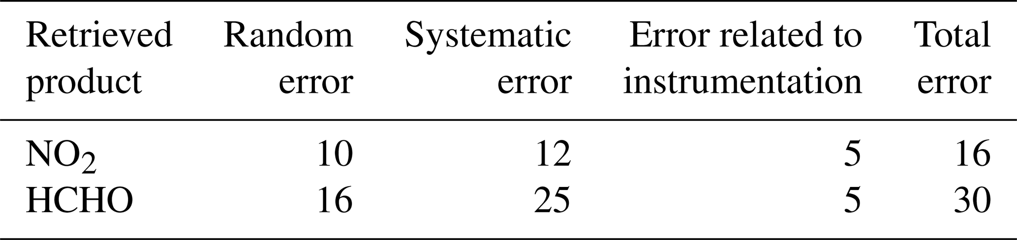
The total error in the retrieval consists of random and systematic errors. The measurement error covariance matrix constructed from the residuals of the respective trace gas ΔSCDs is used to estimate the random error. The systematic error is calculated while assuming uncertainties as high as 30 % and 50 % in the retrieved AOD (or the corresponding Abox values). Table 2 shows the total estimated error. Aside from the random and systematic error, more sources of error might exist. For instance, the bias in the ELs can induce uncertainties in the retrieved products. However, Hoque et al. (2018a) demonstrated that such biases had a non-significant effect on the final retrieved products, mostly less than 5 %.
Table 2Estimated errors (%) for the NO2 and HCHO concentration in the 0–1 km layer, retrieved using the JM2 algorithm.
The cloud-screening procedure is similar to that described by Irie et al. (2011) and by Hoque et al. (2018a, b). During the retrieval steps, retrieved AOD values greater than 3 are excluded because optically thick clouds are primarily responsible for such large optical depth. Filtering based on the residuals of O4 and the trace gas ΔSCDs is also used to screen clouds. Larger residuals likely occur due to two reasons: (1) when the constructed profile is too simple to represent the true profile, particularly with a steep vertical gradient of extinction due to clouds, and (2) rapid changes in optical depth within 30 min (time for one complete scan) (Irie et al., 2011). The screening criteria are respective residuals of O4, HCHO, and NO2 ΔSCDs < 10 %, < 50 %, and < 20 % and the degrees of freedom of retrievals greater than 1.02. The threshold values were determined statistically corresponding to the mode plus 1 sigma (1σ) in the logarithmic histogram of relative residuals.
2.3 CHASER simulations
CHASER 4.0 (version 4) (Sudo et al., 2002; Sudo and Akimoto, 2007; Sekiya and Sudo, 2014), coupled online with the MIROC atmospheric general circulation model (AGCM) and the SPRINTARS aerosol transport model (Takemura et al., 2005, 2009), is a global chemistry transport model used to study the atmospheric environment and radiative forcing. In addition, several updates, including the introduction of aerosol species (sulfate, nitrate, etc.) and related chemistry, radiation, and cloud processes, have been implemented in the latest version of CHASER.
CHASER can calculate the concentrations of 92 species through 263 chemical reactions (gaseous, aqueous, and heterogeneous chemical reactions) considering the chemical cycle of O3–HOx–NOx–CH4–CO along with oxidation of non-methane volatile organic compounds (NMVOCs) (Miyazaki et al., 2017). The chemical mechanism is largely based on the master chemical mechanism (MCM, http://mcm.york.ac.uk, last access: 1 August 2022) (Jenkin et al., 2015). CHASER simulates the stratospheric O3 chemistry considering the Chapman mechanisms, catalytic reactions related to halogen oxides (HOx, NOx, ClOx, and BrOx), and polar stratospheric clouds (PSCs). Resistance-based parameterization (Wesely, 1989), cumulus convection, and large-scale condensation parameterizations are used to calculate dry and wet depositions. The piecewise parabolic method (Colella and Woodward, 1984) and the flux-form semi-Lagrangian schemes (Lin and Rood, 1996) calculate advective tracer transport. CHASER simulates tracer transport on a sub-grid scale in the framework of the prognostic Arakawa–Schubert cumulus convection scheme (Emori et al., 2001) and the vertical diffusion scheme (Mellor and Yamada, 1974). In this study, CHASER simulations were conducted at a horizontal resolution of 2.8∘ × 2.8∘, with 36 vertical layers from the surface to ∼ 50 km altitude and a typical time step of 20 min. The meteorological fields simulated by MIROC AGCM were nudged toward the 6-hourly NCEP FNL reanalysis data at every model time step.
The anthropogenic, biomass burning, lightning, and soil emissions of NOx were incorporated into CHASER simulations. Anthropogenic emissions were based on HTAP_v2.2 for 2008. Biomass burning and soil emissions from the ECMWF MACC (Global Fire Assimilation System, GFAS) reanalysis were used. The biogenic emissions for VOCs are based on the simulations of the process-based biogeochemical model the Vegetation Integrative SImulator for Trace gases (VISIT) (Ito and Inatomi, 2012). The NOx production from lightning is calculated based on the parameterization of Price and Rind (1992) linked to the convection scheme of the AGCM (Sudo et al., 2002). Isoprene, terpene, acetone, and ONMV (non-methane volatile organic compounds) emission estimates in the VISIT inventory during July were 2.14 × 10⁻¹¹, 4.43 × 10⁻¹², 1.60 × 10⁻¹², and 9.93 × 10⁻¹³ kg C m−2 s−1. Global NOx emissions of 43.80 Tg N yr−1 are used in the simulations, considering industries (23.10 Tg N yr−1), biomass burning (9.65 Tg N yr−1), soil (5.50 Tg N yr−1), lightning (5 Tg N yr−1), and aircraft (0.55 Tg N yr−1) as significant sources. Global isoprene emissions from vegetation were set to 400 Tg C yr−1.
NOx emissions in India were estimated as 14 Tg yr−1 in 2016, an almost 2-fold increase since 2005 (∼ 8 Tg yr−1), with the energy and transportation sector being the largest contributor (Sadavarte and Venkataraman, 2014). Indian anthropogenic non-methane VOC (NMVOC) emissions in 2010 were estimated at ∼ 10 Tg yr−1, with contributions of 60 %, 16 %, and 12 % from residential, solvents, and the transport sector, respectively (Sharma et al., 2015). In Japan, vehicular exhausts (14 %–25 %), gasoline vapor (9 %–16 %), liquefied natural gas (7 %–10 %), and liquefied petroleum gas (49 %–71 %) contribute to the total VOC concentrations (Morino et al., 2011), with annual NMVOC emission of ∼ 2 Tg (Kannari et al., 2007). Annual NOx emissions in Japan and Thailand in 2000 were estimated as ∼ 2000 and 591 kt yr−1, with the largest contribution from transport-oil use, followed by the energy and industrial sector (Ohara et al., 2007). Annual anthropogenic VOC emissions in Thailand are approximately 0.9 Tg, with 43 %, 38 %, and 20 % contributed from industrial, residential, and transportation sectors, respectively (Woo et al., 2020).
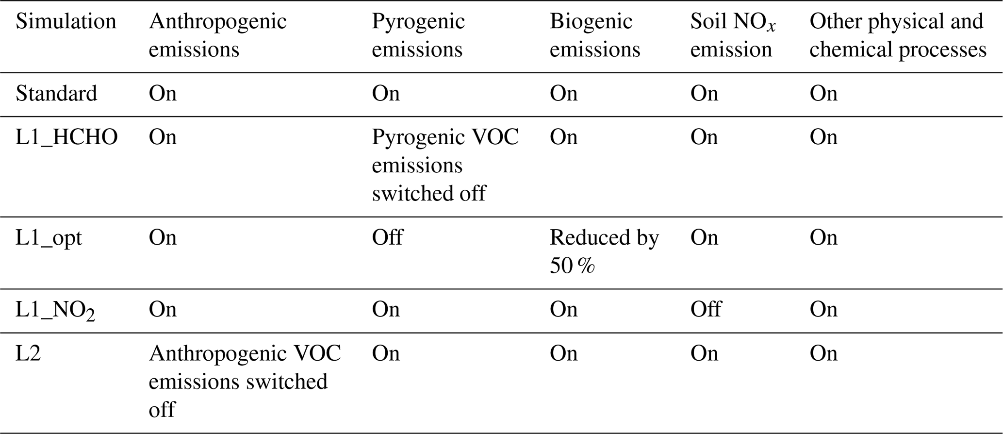
Multiple CHASER simulations with different settings used for sensitivity studies are presented in Table 3.
2.4 Satellite observations
Tropospheric NO2 and HCHO retrievals from the Ozone Monitoring Instrument (OMI) were also used to evaluate the model simulations. The ultraviolet nadir-viewing spectrometer OMI, on board the Aura satellite, measures backscattering solar radiation covering the spectral range of 270–500 nm (Levelt et al., 2006). In an ascending sun-synchronous polar orbit, OMI crosses the Equator at 13:40 LT (local time; Zara et al., 2018). OMI measures at a spatial resolution of 13 × 24 km2 and provides daily global coverage of various trace gases including NO2 and HCHO. The NO2 and HCHO datasets were obtained from the TEMIS (http://www.temis.nl, last access: 23 April 2022) and aeronomie (https://h2co.aeronomie.be/, last access: 3 May 2022) websites, respectively. NO2 tropospheric columns retrieved using the DOMINO version 2.0 (Boersma et al., 2011) algorithm were used for the analysis. Data meeting the following criteria were selected: cloud fraction < 0.5, SZA < 70∘, surface albedo < 0.3, quality flags of 0, and cross-track quality flags of 0. For HCHO, we used the products retrieved with BIRA-IASB v14 (De Smedt et al., 2021). The data-filtering criteria were the following: cloud fraction < 0.4, SZA < 70∘, AMF (air mass factor) > 0.2, quality flag of 0, and cross-track quality flag of 0.
3.1 Results from MAX-DOAS observations
3.1.1 HCHO seasonal variation
The monthly mean HCHO mixing ratios in the 0–1 and 0–2 km layers from January 2017–December 2018 and the corresponding 1-sigma (1σ) standard deviations indicating the variation ranges for the three sites are presented in Fig. 4. The HCHO levels at the Phimai site show a consistent seasonal cycle, characterized by high VMRs during the dry season. Such enhancement is related to the influence of biomass burning during the dry season, which has been well documented in the work of Hoque et al. (2018a). The HCHO mixing ratio at Phimai reaches a peak in March or April, with a maximum of 4–6 ppbv. The variation in the peak concentration and timing depends mainly on the intensity of biomass burning activities. During the wet season, the HCHO concentrations are mostly within 2–3 ppbv, indicating a 2-fold increase in HCHO abundances during the dry season. The daily mean HCHO amounts (0–1 km) are 0.78–9.84 ppbv, representing seasonal modulation of 134 %.
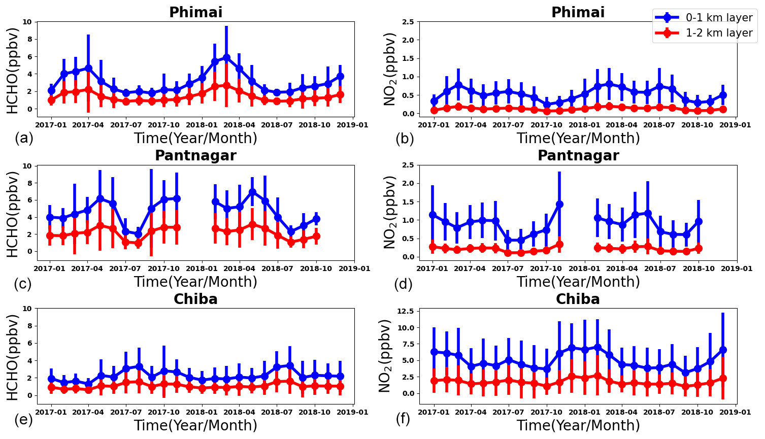
Figure 4Seasonal variations in the HCHO (a, c, e) and NO2 (b, d, f) mixing ratios in the 0–1 (blue) and 1–2 km (red) layers at Phimai, Pantnagar, and Chiba. The error bars represent the 1σ standard deviation of the mean values. The gaps in the plots for the Pantnagar site indicate the unavailability of observations during the investigated period.
Seasonal variation in HCHO in the 0–1 km layer at the Pantnagar site has been elucidated by Hoque et al. (2018b). Here, the results are replotted to verify the consistency of the seasonal variations. Observations made during autumn 2018 were not available because of a problem with the spectrometer. Consistent seasonal variation in HCHO abundances is observed at the Pantnagar site, with enhanced concentrations during the spring. The Pantnagar site is affected by biomass burning during spring and autumn (Hoque et al., 2018b), explaining the high mixing ratios found during spring. In both years, the maximum HCHO mixing ratios are ∼ 6 ppbv. The springtime peak occurred in May. The HCHO concentrations during the monsoon are ∼ 35 % lower than in the spring, indicating a strong effect of the monsoon on the HCHO concentrations found for Pantnagar. The seasonal modulation of HCHO at Pantnagar estimated from the daily mean concentrations is 107 %. The peak HCHO mixing ratio at Pantnagar is almost twice that in the city of Pune (∼ 3 ppbv) (Biswas and Mahajan, 2021), a site in the IGP region. The HCHO seasonality is found to be dissimilar at the two sites because of differences in the VOC sources; however, lower mixing ratios during the monsoon are consistent. From another site in the IGP region (i.e., Mohali), Kumar et al. (2020) reported the lowest HCHO VCDs during March 2014 and 2015, attributing them to lower biogenic and anthropogenic VOC emissions. At Pantnagar, the lowest HCHO mixing ratios are observed during the monsoon. The rainfall events in the IGP region shows strong annual variability (Fukushima et al., 2019). Discrepancies between the sites might be related to the rainfall pattern.
Under the influence of biomass burning, the maximum monthly HCHO mixing ratios at Phimai and Pantnagar are similar (∼ 6 ppb). The maximum instantaneous HCHO VMR during biomass burning influence in Phimai and Pantnagar is 26 and 30 ppbv, respectively. Zarzana et al. (2017) reported HCHO abundances of ∼ 60 ppbv in fresh biomass plumes in the USA. The lower values obtained from our measurements might be attributable to (1) more aged plumes intercepted by the MAX-DOAS instruments and (2) differences in the types of biomass fuel used. Comparison to reports in the literature indicates that the retrieval of HCHO under biomass burning is reasonable.
The summertime maximum and wintertime minimum characterize the seasonal variations in HCHO at the Chiba site, with a peak at ∼ 3 ppbv. The HCHO concentrations are ∼ 2 ppbv during other seasons, which are similar to the HCHO concentrations in Phimai during the wet season. The seasonal variation amplitude of HCHO at Chiba is ∼ 94 %. For a site with similar seasonal variation (i.e., summertime maximum and wintertime minimum), Franco et al. (2015) reported HCHO seasonal modulation of 88 %.
The HCHO VMRs in the 1–2 km layers at all three sites are lower, almost 50 % the value of the concentrations in the 0–1 km layer. The HCHO seasonal variation amplitudes at the Phimai, Pantnagar, and Chiba sites are 131 %, 102 %, and 90 %, respectively, when calculated based on the HCHO concentration in the 1–2 km layers. The modulation was even lower when retrieved values for the 2–3 km layer were used.
3.1.2 NO2 seasonal variation at the three sites
Figure 4 also shows the seasonal variation in NO2 in the 0–1 and 1–2 km layers at the three sites. The error bars represent the 1σ standard deviation of the mean values. The NO2 seasonal variations at Phimai and Pantnagar sites are similar to those of HCHO. Pronounced peaks attributable to biomass burning influence are observed during the dry season at Phimai (∼ 0.8 ppbv) and during spring (1.2 ppbv) and post-monsoon (1.4 ppbv) at Pantnagar. The lowest NO2 mixing ratios at Phimai and Pantnagar are ∼ 0.2 and 0.5 ppbv, respectively. The NO2 VMRs at Chiba are higher (∼ 7 ppbv) during winter. The longer lifetime of NOx and lower NO NO2 ratio because of lower photochemical activity in winter lead to high NO2 mixing ratios at Chiba (Irie et al., 2021).
At Phimai, the NO2 mixing ratios in both seasons are similar. However, when Hoque et al. (2018a) reported the seasonal variations in NO2 at Phimai during 2015–2018, the dry-season mixing ratios were higher. Table 4 shows the number of fire events during the dry seasons during 2015–2018. The fire data are extracted from the MODIS Active Fire Data (https://firms.modaps.eosdis.nasa.gov, last access: 15 December 2021). Data fulfilling the following criteria were chosen – (a) data points located within 100 km of the Phimai site, (b) confidence in the data greater than 70 %, and (c) observations during the daytime. The lower fire counts during 2017–2018 compared to those of the 2015–2016 period coincide with the lower NO2 levels in the former. Fire counts varied between 2017 and 2018 but did not affect the NO2 levels. However, HCHO levels changed with the number of fire occurrences between 2015–2018 (i.e., Fig. 4 and Hoque et al., 2018a).
Table 4Number of fire events occurring during the dry season (January–April) at Phimai from 2015–2018. Selection criteria of the data are the following: (1) situated within 100 km of the site, (2) confidence level > 70 %, and (3) daytime measurements.

At such low NO2 levels at Phimai, soil NOx emissions are likely to make a greater contribution to NO2. Although NO2 is not emitted directly from soils, biological processes emit NO, which is rapidly converted to NO2 (Hall et al., 1996). In addition, many studies have established a relation between soil moisture and NO emissions (Cárdenas et al., 1993; Zheng et al., 2000; Schindlbacher et al., 2004; Huber et al., 2020). The potential contribution of soil NOx emissions, as inferred from CHASER simulations, is discussed in Sect. 3.4.2.
3.1.3 Ozone sensitivity at the three sites
The HCHO-to-NO2 ratio (RFN)
The HCHO-to-NO2 ratio (RFN) is regarded as an indicator of high ozone O3 sensitivity (Martin et al., 2004; Duncan et al., 2010). The O3 production regime is characterized as VOC-limited for RFN < 1 and NOx-limited when RFN > 2, and the values in the range 1–2 are said to be in the transition/ambiguous region (Duncan et al., 2010; Ryan et al., 2020). Subsequent to a report of Tonnesen and Dennis (2000), several studies used RFN estimated from satellite and ground-based observations to infer O3 sensitivity to NOx and VOCs (Martin et al., 2004; Duncan et al., 2010; Jin and Holloway, 2015; Mahajan et al., 2015; Irie et al., 2021; etc.). However, the effectiveness of RFN is still under discussion primarily based on two points – (1) the range of the transition region to categorize the VOC- and NOx-limited region and (2) the altitude dependence of RFN (Jin et al., 2017). Most of the studies described above used the transition range (1 < RFN < 2) proposed by Duncan et al. (2010). Schroeder et al. (2017) reported that a common transition range (i.e., 1 < RFN < 2) might not be valid globally. Instead, it should be calculated based on the region. First, the results based on the standard transition range are discussed herein, and then its applicability to the study regions is assessed.
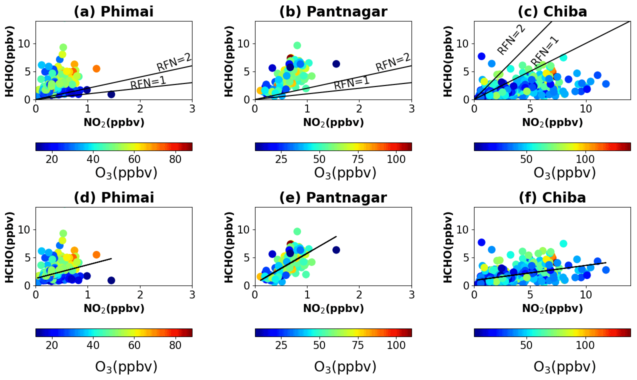
Figure 5Scatterplots of HCHO and NO2 concentrations in the 0–2 km layer at (a, d) Phimai, (b, e) Pantnagar, and (c, f) Chiba, colored with the O3 concentrations in the 0–2 km layer at the respective sites. The solid lines in panels (a)–(c) represent RFN = 2 and RFN = 1 benchmarks. The black lines in panels (d)–(f) are calculated according to Eq. (1).
Figure 5 shows scatterplots of the daily mean NO2 and HCHO concentrations in the 0–2 km layer at the three sites, color-coded with the respective O3 concentrations (0–2 km). Retrieval of the JM2 O3 product is explained by Irie et al. (2011). The O3 concentrations for SZA < 50∘ are used to minimize stratospheric effects. This criterion for the SZA is also applied to the selection of the NO2 and HCHO concentrations. Although not checked here, the JM2 O3 product showed good agreement with ozonesonde measurements in Tsukuba (Irie et al., 2021). Most of the high-O3 occurrences fall in the RFN > 2 region at Phimai and Pantnagar and in the RFN < 1 region at Chiba. The common transition range classifies the O3 production regime as NOx-limited at Phimai and Pantnagar and VOC-limited at Chiba. At all sites, the RFN values tend to be biased toward a particular regime (i.e., NOx- or VOC-limited), with only 4 % and 2 % of the ratios in the range 0–2 at Phimai and Pantnagar, respectively. This finding suggests that the transition occurs at a higher or lower ratio than the common definition. A recent report by Souri et al. (2020) found that the NO2–HCHO relation plays an important role in determining the transition region, and they derived a formulation from accounting for the NO2–HCHO chemical feedback in the ratios as
where m and b denote the slope and intercept, respectively. Equation (6) is based on observations, which means that the regionally adjusted fitting coefficients will reflect the local NO2–HCHO relation. Solving Eq. (6), the transition line estimated from the observations in the 0–2 km layer is shown in Fig. 5 (bottom panels). Rather than a range, the method calculates a single transition line, which corresponds to the NO2–HCHO feedback. The regions above and below the transition line are characterized as VOC- and NOx-limited or other, respectively.
The revised transition line at Phimai and Pantnagar is apparently more reasonable than that of the earlier method. At Phimai, the transition line almost clearly distinguishes between the high- and low-O3 occurrences. It is perceptible that when the HCHO concentrations are higher than NO2, the transition of the regimes is likely to occur at higher RFN values. The minimum and mean RFN values along the transition line are 3.62 and 6.78, respectively. Because Phimai is a VOC-rich environment, the regime transition occurs at higher RFN values than it does by the conventional definition. This finding echoes the results reported by Schroeder et al. (2017) for a regionally variable transition region. The definition of RFN < 1 as a VOC-limited regime might not be valid in this case. Considering the mean RFN ratio along the transition line (i.e., 6.78), the VOC- and NOx-limited (and other) regimes are defined as RFN < 6.78 and RFN > 6.78, respectively. Based on this definition, around 34 % (65 %) of the ratios are higher (lower) than 6.78, classifying Phimai as a dominant VOC-limited region, which contradicts earlier results. Biomass burning affects Phimai during January–April and is a significant emission source in addition to biogenic emissions. Thus, high-O3 occurrences likely occur only 30 % of the time during a year. Such events mostly lie above the transition line.
At Pantnagar, high-O3 occurrences lie below (42 %) and above (57 %) the transition line, indicating that O3 production is sensitive to both HCHO and NO2, which contradicts results reported by Biswas et al. (2019). Based on satellite and ground-based observations, the study estimated the RFN values at a site in the IGP as > 4 and > 2, respectively, and regarded the O3 regime as NOx-limited. Mahajan et al. (2015) reported RFN values of less than 1 over the IGP region, signifying a VOC-limited region. Pantnagar is a sub-urban site situated beside a busy road. Therefore, effects of anthropogenic emissions are expected year-round, especially with pyrogenic emissions during the spring and post-monsoon period. O3 sensitivity to both NOx and VOCs in the northwest IGP region has also been reported by Kumar and Sinha (2021). Therefore, the balance between the VOC- and NOx-limited regions in the IGP is reasonable. The mean and minimum RFN values along the transition line are 5.59 and 6.09, respectively. The minimum value (i.e., 5.59) is higher than in Phimai (3.26), suggesting higher VOC levels at Pantnagar, consistent with the observations.
At Chiba, 60 % of the RFN values lie below the transition line, suggesting a dominant VOC-limited region, which is consistent with the results reported by Irie et al. (2021). The minimum and the mean RFN values along the transition line are 0.33 and 0.72, respectively. The transition occurs at a low RFN value because of higher NO2 levels. The fact that 40 % of the RFN values are above the transition region suggests a moderate effect of HCHO on the O3 sensitivity at Chiba.
Although the new classification results are apparently reasonable, they should be interpreted with care. Our current understanding of RFN contradicts the classification of rural sites as VOC-limited. Despite the theoretical and observational evidence (i.e., Souri et al., 2020), the classification of regimes based on a single transition line is not yet well established. Schroder et al. (2017) used regionally varying transition ranges. Moreover, (a) the number of observations and (b) the systematic and retrieval errors can affect the estimations and classifications. These findings are expected to contribute to the ongoing discussion about the effectiveness of RFN. However, the results support the idea of a regionally varying transition range.
RFN profiles
Figure 6 shows the seasonal mean RFN profiles at the three sites. Only the profiles during the high O3 concentrations at the sites (i.e., March at Phimai, May at Pantnagar, and February at Chiba) are shown. The RFN values likely increase with height because of the lower vertical gradient of NO2 than that of HCHO (Fig. 4). It is particularly interesting that the RFN values are similar at the 1–2 km height under biomass burning conditions, suggesting a small variation in the HCHO loss rate in the particular layer. At both sites, the HCHO concentration at 1.5 km is about 3 ppbv. At Chiba, a considerable amount of NO2 in the higher layers increases the ratio up to a 2 km height. Beyond 2 km, the ratio variation at all sites is the opposite of that found for the surface. The gradient issue of RFN has been discussed explicitly by Jin et al. (2017). They proposed a conversion factor to account for gradient differences in the surface and column-derived RFN values, estimating the conversion factor from the model-simulated surface and column abundances of NO2 and HCHO. We adopt the method reported by Jin et al. (2017) for this study using the CHASER-simulated NO2 and HCHO concentrations and vertical columns.
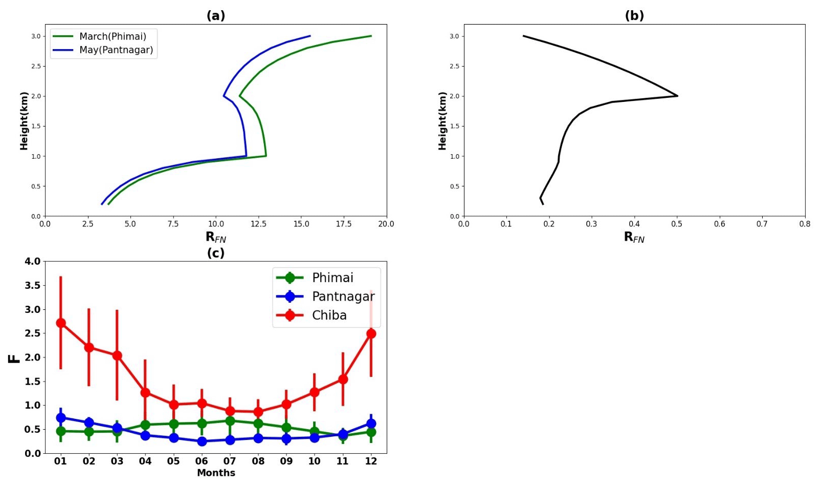
Figure 6Seasonal mean RFN profiles during (a) March and May at Phimai and Pantnagar, respectively, and (b) February at Chiba. (c) Seasonal variations in the column-to-surface conversion factor (F) for the Phimai, Pantnagar, and Chiba sites, estimated from the CHASER-simulated HCHO and NO2 surface concentrations and VCD. The simulated data from 07:00–18:00 LT in 2017 were used to estimate the F values. The error bars represent the 1σ standard deviation of the mean values.
First, CHASER-simulated near-surface NO2 and HCHO concentrations were converted to number density. The effective boundary layer height (E) (Halla et al., 2011; Jin et al., 2017) was estimated.
Therein, and EHCHO denote the effective boundary layer heights of NO2 and HCHO, respectively.
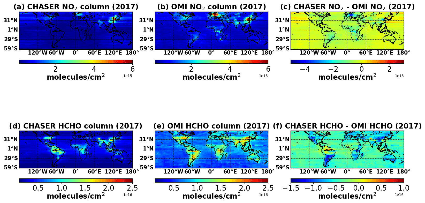
Figure 7(a–c) Annual mean tropospheric NO2 (× 1015 molecules cm−2) columns (a) simulated by CHASER and (b) retrieved from OMI observations. Only limited NO2 data in July and December met the filtering criteria; thus they were discarded from the calculation. (c) The differences between the simulated and observed NO2 columns. (d–f) Annual mean HCHO (× 1016 molecules cm−2) columns (d) simulated by CHASER and (e) retrieved from OMI observations. (f) The differences between the simulated and observed HCHO columns. Only the data for 2017 are plotted. All the datasets are mapped onto a 2.8∘ bin grid.
In the second step, the column-to-surface conversion factor (F) was calculated according to the following equation:
The seasonal variation in F for the three A-SKY sites and the associated 1σ standard deviation of the mean values are depicted in Fig. 7c. The F values over East Asia reported by Jin et al. (2017) were ∼ 2, without marked seasonal variation. CHASER-estimated F values over Chiba range between 1–2.5, which is apparently reasonable when compared with literature values. Values reported in the literature for polluted regions (NO2 > 2.5 molecules cm−2) considered simulation data for 13:00–14:00 LT, but the estimates for this study used daytime (07:00–18:00 LT) simulations.
The F values for Pantnagar are mostly less than 1, with no distinctive seasonal variation. Mahajan et al. (2015) reported OMI-derived RFN values < 1 over the IGP region. When this estimated conversion factor is used with the values reported by Mahajan et al. (2015), the discrepancy in the satellite and ground-based observation-derived RFN values in the IGP region is reduced, indicating that the estimated F values for the Pantnagar site can be representative of the IGP region. The F values at the Phimai site were 0.5–1. Our estimated F values for the Phimai and Pantnagar sites are useful as representative values for these respective regions, which can be improved further based on the results.
3.2 Global evaluation of the CHASER model
This section describes the evaluation of CHASER NO2 and HCHO columns for 2017 against OMI observations. The OMI AKs were applied to the CHASER outputs to account for the altitude dependence of the retrievals. First, 2-hourly simulated profiles (NO2 and HCHO) were sampled closest to the observation time. Secondly, AKs were applied to the sampled profiles and the mean profile was calculated. Thirdly, both the simulations and the observations were averaged on a 2.8∘ bin grid. The months of July and December were discarded from the NO2 comparison because few coincident days (only 5 d) were available after filtering. It should be noted that simulations based on old NOx emission inventories will likely affect the model–satellite comparison results. However, the current study has not assessed such an impact due to technical issues related to using an updated emission inventory. All these issues will be addressed in a separate study.
3.2.1 Comparison between CHASER and OMI NO2
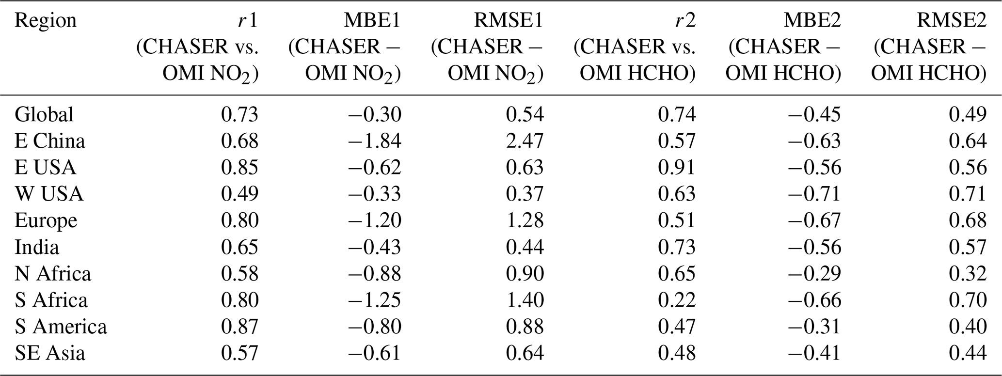
Figure 7 compares the simulated and observed annual mean tropospheric NO2 columns. The statistics for the comparison are given in Table 5. The model captured the global spatial variation well with a spatial correlation (r) of 0.70. The mean bias error (MBE) and the root mean square error (RMSE) are 3 × 10¹⁴ and 5.4 × 10¹⁴ molecules cm−2, respectively. On a global scale, CHASER estimations are negatively biased by 38 % compared to OMI. Previous studies evaluating global NO2 simulations with satellite observations have reported similar negative biases (Miyazaki et al., 2012; Sekiya et al., 2018). The differences in the spatial representativeness between the model and observations constitute one potential reason for such negative biases. CHASER simulations at 1.1∘ improved the MBE and RMSE by 5 % and 15 %, respectively, compared to simulations at 2.8∘ (Sekiya et al., 2018). Moreover, Sekiya et al. (2018) used NO2 simulations with an updated inventory and compared the results with OMI observations from 2014. Although they reported a better global spatial correlation (r > 0.90), the MBE (2.5 × 10¹⁴ molecules cm−2) and RMSE (4.4 × 10¹⁴ molecules cm−2) values at 2.8∘ resolution are comparable to those obtained from this study.
Table 5Statistics of comparison of annual mean NO2 and HCHO columns between CHASER and OMI. MBE1 and MBE2 are the respective mean bias errors. RMSE1 and RMSE2 are the respective root mean square errors. r1 and r2 signify the respective spatial correlation coefficients. The units of MBE1 and RMSE1 are × 1015 molecules cm−2. MBE2 and RMSE2 values are in the units of × 1016 molecules cm−2.
OMI retrievals show the highest NO2 columns over eastern China (E China) and western Europe. Annual mean NO2 columns over the remainder of the land areas are between 7 × 10¹⁴ and 4 × 10¹⁵ molecules cm−2. Over the land areas the differences between the datasets are mostly between −2 × 10¹⁵ and 5 × 10¹⁴ molecules cm−2. Although CHASER also underestimates NO2 columns over the ocean, the differences are lower than those over lands. CHASER estimates are higher by ∼ 5 × 10¹⁴ molecules cm−2 than OMI over Japan. Since 2012, the NO2 columns have shown a declining trend over Japan, mainly because of emission controls in China (Irie et al., 2016). Probably because of simulations with an emission inventory earlier than 2012, the simulated values tend to be higher than observations.
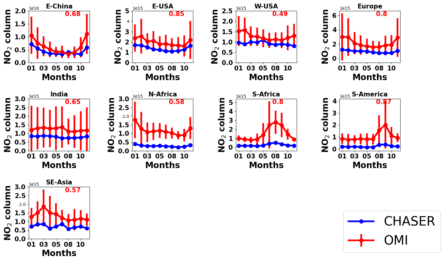
Figure 8Seasonal variations in tropospheric NO2 columns in E China (30–40∘ N, 110–123∘ E), E USA (32–43∘ N, 71–95∘ W), W USA (32–43∘ N, 100–125∘ W), Europe (35–60∘ N, 0–30∘ E), India (7.5–54∘ N, 68–97∘ E), N Africa (5–15∘ N, 10∘ W–30∘ E), S Africa (5–15∘ S, 10–30∘ E), S America (0–20∘ S, 50–70∘ W), and SE Asia (10–20∘ N, 9–145∘ E). CHASER simulations and OMI retrievals are plotted in blue and red colors, respectively. The error bars indicate the 2σ variation in the observed mean values. The number in each panel signifies the regional spatial correlation between CHASER and OMI NO2 columns.
Figure 8 compares the seasonal variations in the monthly mean NO2 columns in some selected regions. The error bars represent the 2σ standard deviation of the observed mean values. The numbers in each subplot signify the regional spatial correlation between the datasets. Over eastern China (E China), CHASER values are negatively biased by 24 %; the r value is 0.68. The model captured the seasonality well within the variation range of the observations. Over E and W USA (eastern and western USA), the r values are 0.85 and 0.49, respectively. Simulated NO2 columns are higher over E USA than over W USA, consistent with the observations. Although in both regions model estimates are biased by ∼ 23 % on the lower side compared to OMI observations, the RMSEs in E USA are ∼ 40 % higher than in W USA.
Over Europe, CHASER estimates are negatively biased by 54 %, with an r value and RMSE of 0.80 and 1.28 × 10¹⁵ molecules cm−2, respectively. The observed NO2 levels over Europe are almost twice those of W USA. The model was unable to capture the regional differences. Model underestimations in Europe can be attributed to the older anthropogenic emission inventory used for the study. In fact, using the HTAP 2010 inventory, the MBE (−0.53 × 10¹⁵ molecules cm−2) between OMI and CHASER NO2 column simulations at 2.8∘ over Europe (Sekiya et al., 2018) was ∼ 50 % lower than in the current study, although their RMSE value was similar.
Over India, MBE and RMSE for the annual mean NO2 column are −4.3 × 10¹⁴ and 4.4 × 10¹⁴ molecules cm−2, respectively, and the r value is moderate (0.65). Although CHASER estimates are negatively biased by 32 %, the values lie within the 2σ range of the observations. Sekiya et al. (2018) found no significant effect of higher model resolution on the MBE and RMSE in the Indian region.
Over N and S Africa (northern and southern Africa), the model values are biased low by more than 75 % compared to the observations. Prominent biomass burning occurs in both regions, which explains the enhanced NO2 levels in the OMI retrievals. High negative biases in the model values indicate that biomass burning NOx emissions for the African regions are likely underestimated. Similarly, CHASER underestimates NO2 columns by 80 % in South America, where pyrogenic emissions contributions are significant. CHASER estimates are lower than OMI in these regions, but the model captured the spatial distribution well.
Over the SE Asian (southeast) region, OMI columns are enhanced during the dry season (i.e., January–April). Burning agricultural waste is a common practice in many countries in Southeast Asia during the dry season, explaining the enhanced columns. The MBE (−6 × 10¹⁴ molecules cm−2) and RMSE (6.4 × 10¹⁴ molecules cm−2) in the SE Asia region are lower than in the African regions (i.e., N Africa, S Africa, and S America), where biomass burning is prominent.
3.2.2 Comparison between CHASER and OMI HCHO
Figure 9 presents a comparison between the simulated and observed global annual mean HCHO columns. The statistics of the comparison are given in Table 5. CHASER is able to reproduce the observed global spatial variation well with r = 0.73. The global MBE and the RMSE are −4.5 × 10¹⁵ and 4.9 × 10¹⁵ molecules cm−2, respectively. MBE and RMSE for monthly mean fields show no distinctive seasonal variation (Table S2). High HCHO columns are observed over China, Australia, Europe, India, central Africa, South America, and the United States. The model mostly underestimated the HCHO abundances in the higher latitudes and Australia. Absolute differences between the model and observations in the higher latitudes vary between 5 × 10¹⁵ and 1 × 10¹⁶ molecules cm−2. Figure 9 compares the seasonal variations in the monthly mean HCHO columns in some selected regions. Therein error bars represent the 2σ standard deviation of the observed mean values. The numbers in the respective subplots signify the regional spatial correlation between the datasets.
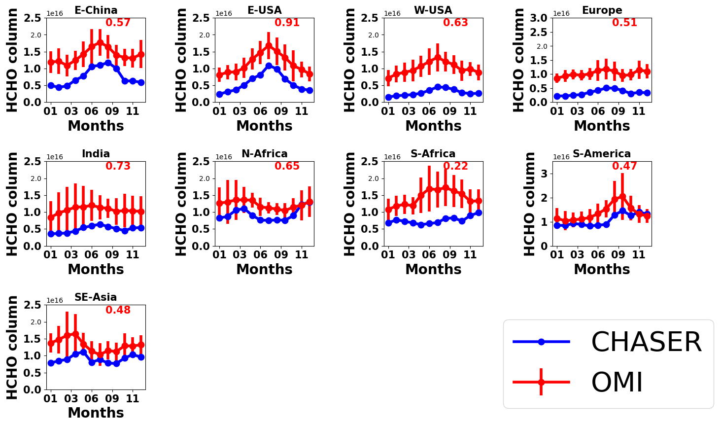
Figure 9Seasonal variations in HCHO columns in E China (30–40∘ N, 110–123∘ E), E USA (32–43∘ N, 71–95∘ W), W USA (32–43∘ N, 100–125∘ W), Europe (35–60∘ N, 0–30∘ E), India (7.5–54∘ N, 68–97∘ E), N Africa (5–15∘ N, 10∘ W–30∘ E), S Africa (5–15∘ S, 10–30∘ E), S America (0–20∘ S, 50–70∘ W), and SE Asia (10–20∘ N, 9–145∘ E). CHASER simulations and OMI retrievals are plotted in blue and red colors, respectively. The error bars indicate the 2σ variation in the observed mean values. The number in each panel signifies the regional spatial correlation between CHASER and OMI HCHO columns.
Over E China, CHASER HCHO estimates are negatively biased by 45 % compared to OMI, and the r value is greater than 0.50. The model reproduced the observed HCHO seasonality well including enhanced peaks during the summer. The greatest differences between the datasets are observed during the winter. Over E USA, the spatial correlation between the datasets is greater than 0.90. Also, the CHASER estimates are biased by 49 % on the lower side. Simulations show that the peak in the HCHO abundances occurs in July, which is consistent with the observations. The observed and simulated magnitude of the seasonal modulation is 51 % and 78 %, respectively. The seasonality in the HCHO columns in E China and E USA signifies a strong contribution from biogenic emissions. In both regions, the observed peak HCHO column is ∼ 1.75 × 10¹⁶ molecules cm−2. The simulated peak HCHO values are also similar in both regions, despite the underestimation. Over W USA and Europe, the negative biases in the simulation are greater than 60 %. However, the simulated peaks during summer are consistent with the observations. The OMI retrievals show that the HCHO abundances in both regions are almost similar, which has been well captured by CHASER, although the magnitude is underestimated.
Over India, the model estimates mostly lie outside of the observational variation ranges, although CHASER captured the spatial distribution well (r = 0.73). Magnitudes of the seasonal variation in both OMI and CHASER are around 32 %. Between the two African regions, CHASER demonstrated better capability for reproducing HCHO distribution in N Africa (r = 0.65). Negative model bias in N Africa is almost half (22 %) that of S Africa (46 %). Observed N African HCHO columns are mostly higher than 1.2 × 10¹⁶ molecules cm−2 during the biomass burning period (November–April). Although the modeled values are lower than the observed values, the year-end columns (November–December) are similar. Both datasets show low HCHO variation during May–September. Over the S African region, the model capabilities were limited.
Over S America, the negative bias (∼ 22 %) in the model estimates compared to the observations is similar to that of N Africa. In addition to consistency in the year-end (November to December) columns, CHASER well reproduced the biomass-burning-led enhancements. The observed and simulated magnitudes of seasonal modulation are 49 % and 43 %, respectively.
Over SE Asia, CHASER reproduced the observed biomass-burning-led enhanced HCHO columns during the dry season (January–April); however, the occurrence of the peak is inconsistent. As discussed in Sect. 3.1, observed HCHO peaks related to biomass burning can vary depending on the fire numbers. The r value (0.48) is moderate, and the model is biased by 30 % on the lower side. The model negative biases in the biomass-prone regions are the lowest (< 30 %) among the discussed regions.
De Smedt et al. (2021) reported that cloud corrections can positively bias OMI HCHO columns by up to 30 % compared to TROPOspheric Ozone Monitoring Instrument (TROPOMI) columns. Consequently, uncertainties in the observations are also likely to contribute to the observed negative biases. Comparison among CHASER, TROPOMI, and OMI HCHO columns is beyond the scope of this study. However, the effects of uncertainties in the satellite retrievals on the negative biases are discussed qualitatively and briefly. To demonstrate such effects, CHASER and TROPOMI HCHO columns for 2019 are compared in Fig. S3. The simulation settings and emission inventories are similar to those explained in Sect. 3.2.3. The comparison results are presented in Table S2. TROPOMI data have been processed following De Smedt et al. (2021). The CHASER and TROPOMI HCHO spatial distribution correlates strongly, with an r value of 0.78. The values for MBE and RMSE are −2.3 × 10¹⁵ and 2.8 × 10¹⁵ molecules cm−2, respectively. Compared to OMI and TROPOMI, CHASER HCHO columns are negatively biased by 61 % and 38 %, respectively. The model biases are lower when compared to TROPOMI observations. Because of temporal differences in the two comparisons, the biases cannot be compared quantitatively. However, the differences in the biases signify that the observational uncertainties can strongly affect discrepancies between the simulated and observed HCHO abundances. Moreover, using different cloud products may introduce inconsistencies into the OMI BIRA-IASB retrievals (De Smedt et al., 2021), affecting the comparison results. De Smedt et al. (2021) proposed recalculating the OMI HCHO VCDs based on the AMF information to minimize cloud-induced uncertainties. Such a detailed method will be evaluated in our future studies.
3.3 Evaluation of CHASER simulations at the three sites
3.3.1 Evaluation of CHASER HCHO at Phimai and Chiba
The seasonally averaged observed and modeled HCHO profiles and partial columns in the 0–4 km altitude range at Phimai and Chiba are presented in Fig. 10. The CHASER outputs smoothed with MAX-DOAS averaging kernels (AKs) are also depicted. The AK is applied following Franco et al. (2015). First, the CHASER HCHO profiles are interpolated to the MAX-DOAS vertical grids. Next, the MAX-DOAS AK information from individual retrieved profiles is seasonally averaged according to the climate classifications of each site. Finally, the CHASER outputs on the coincident days are selected, and the seasonally averaged AK is applied to the daily mean interpolated profile. Applying individual AKs to the model outputs yielded similar results. The seasonally averaged AKs for both sites are shown in Fig. S4. The coincident days at Phimai and Chiba were 690 and 668, respectively.
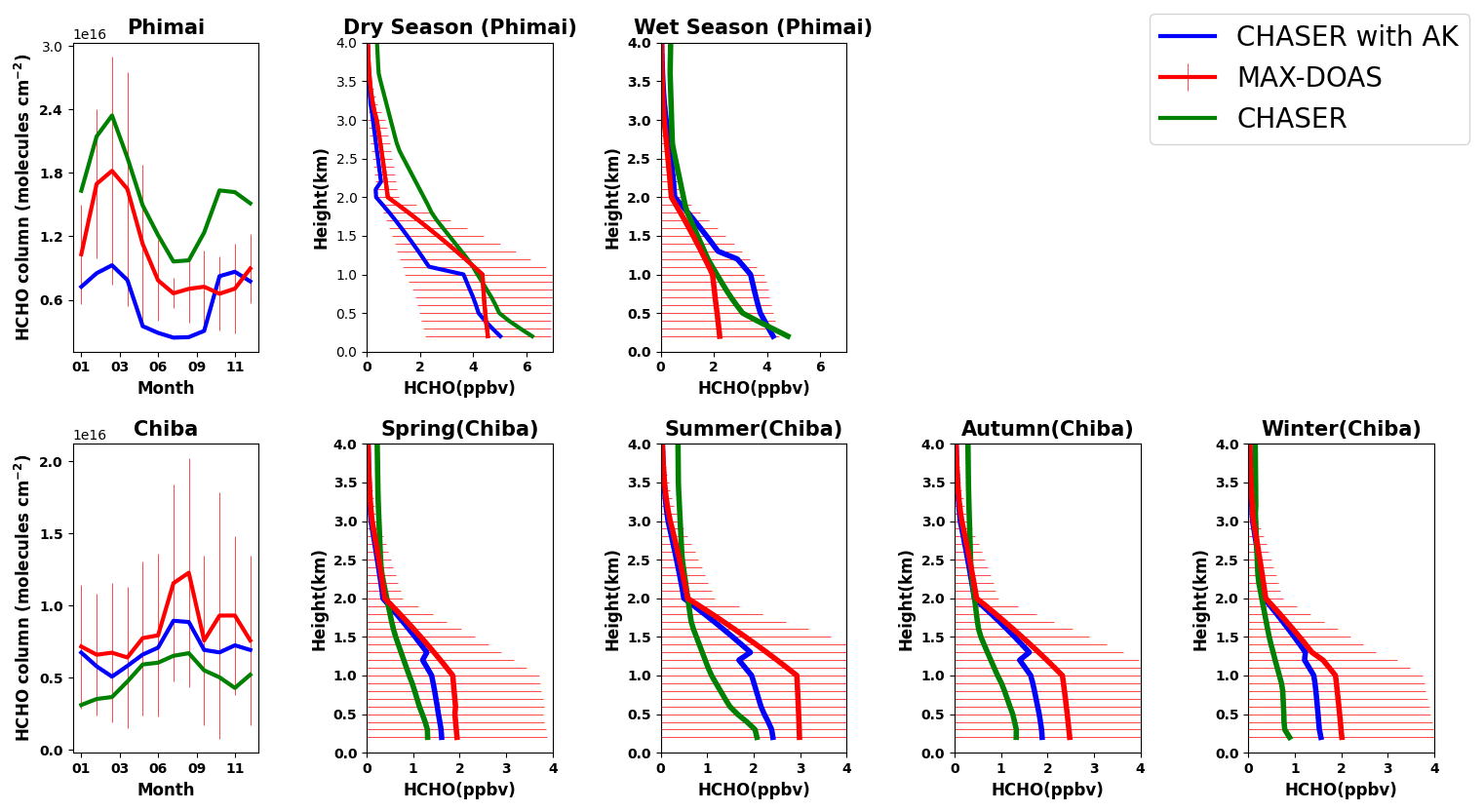
Figure 10Seasonal variations in the HCHO partial columns at 0–4 km and vertical profiles during all seasons at Phimai and Chiba, as inferred from the MAX-DOAS observations (red) and CHASER simulation (green). The CHASER HCHO partial column and vertical profile smoothed with the MAX-DOAS AK are colored blue. The AK information of all the screened (as explained in Sect. 2.2) retrievals was averaged based on the seasonal classification of the respective sites. Only the coincident time and date between the model and observations are selected. Error bars indicate the 1σ standard deviation of mean values of the MAX-DOAS observations.
Table 6Comparison of the seasonal mean HCHO partial columns and profiles (0–4 km) between MAX-DOAS and CHASER at Phimai and Chiba. MBE (CHASER − MAX-DOAS) is the mean bias error. The partial-column and profile MBE units are × 1016 molecules cm−2 and parts per billion by volume (ppbv), respectively.
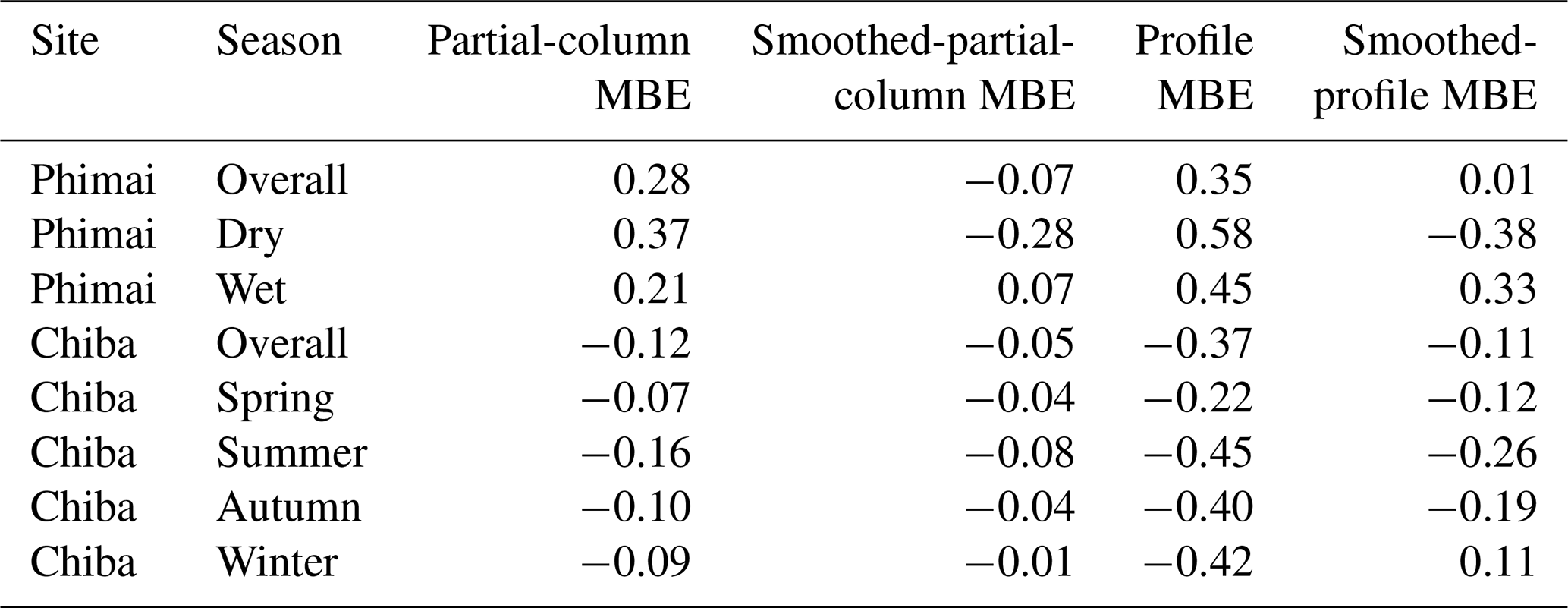
At Phimai, CHASER predicted the increase in the HCHO partial columns during the dry season and well reproduced the HCHO seasonality. The simulated and observed seasonality correlates strongly, with an r value of 0.96. The modeled monthly mean values during the dry season are found to be within the 1σ standard deviation of the observed values, indicating that the pyrogenic emission estimates used for the simulations are reasonable. CHASER predicted a 41 % increase in the HCHO column during January–March, consistent with the observations (41 %). CHASER overestimates the HCHO columns in both seasons, and the mean bias error (MBE) (CHASER − MAX-DOAS) is lower (3.7 × 10¹⁵ molecules cm−2) (Table 6) during the wet season. Although underestimated, the dry-season smoothed column values are within the 1σ range.
The modeled and observed HCHO mixing ratios in the 1–2 km layers during the wet season are almost identical, whereas VMRs near the surface (i.e., 0–1 km) differ by 30 %. The absolute mean difference in the 0–4 km layer is ∼ 0.45 ppbv, with a maximum difference of 2.58 ppbv below 200 m. CHASER has demonstrated good capabilities for reproducing the HCHO profile in the 0.5–4 km layer during the wet season. The significance of AK information is low for the wet season. However, smoothing the model profiles reduces the overall MBE by 43 %.
During the dry season, the respective absolute mean and maximum difference in the datasets in the 0–1 km layers is ∼ 1 and ∼ 2 ppbv. The observed and simulated seasonal differences in the 0–1 km are 50 % and 34 %, respectively. Simulated dry-season profile values at the heights greater than ∼ 2 km are out of the 1σ variation range. The two potential reasons for such differences are lower measurement sensitivity in the free troposphere and the overestimated Southeast Asian biogenic emissions in the model. Despite the measurement limitations, CHASER and MAX-DOAS wet-season profiles up to 3 km are consistent. Consequently, it is likely that the biogenic emissions for this region in the model are overestimated. The Southeast Asian isoprene emissions in CHASER are 128 Tg yr−1, higher than the CAMS-GLOB-BIO (Sindelarova et al., 2022) inventory (78 Tg yr−1). However, the dry-season HCHO profiles in 0–2 km are well simulated. Smoothing underestimates the dry-season profile within the 1σ variation range but improves simulations below 200 m. At heights greater than 3 km, the smoothed values mostly reproduce the a priori because of reduced measurement sensitivity (i.e., low AK value, indicating limited information was retrievable).
Moderate correlation (R=0.58) can be observed between the modeled and observed HCHO partial columns at Chiba. CHASER was able to reproduce the peak in the partial columns in August. The model predicts a 41 % increase in the HCHO columns during January–August, whereas the observed increase is 54 %. Although Chiba is an urban site, the HCHO and temperature seasonal variations show a tight correlation (R ∼ 0.70) (Fig. S5), suggesting that changes in biogenic emissions modulate HCHO seasonality. Similarly, the modeled seasonality is consistent with temperature variation (Fig. S4). Thus, the simulated HCHO seasonality in Chiba is reasonable, despite underestimation of absolute values. Smoothing the simulations improves the correlation, and the MBE is reduced by 54 % (Table 6).
The CHASER HCHO profiles in the 0–4 km layers are lower than the observations, with an MBE of 0.39 ppbv. The absolute differences in the modeled and retrieved HCHO profiles in the 0–2 km layer during all seasons are higher than at Phimai. Absolute mean differences of ∼ 1 pbbv and higher are mainly observed for 0 to 2 km. In addition, the vertical gradients of the simulated profiles are low compared to those at Phimai. The modeled profiles at Chiba resemble the HCHO profiles measured over the ocean during the INTEX-B (Intercontinental Chemical Transport Experiment – Phase B) (Boeke et al., 2011). The Chiba site is near the sea, and the coarse CHASER resolution includes the ocean pixels. Moreover, urban surfaces are not homogeneous. Thus, a significant part of the profile discrepancies are likely related to the systematic differences, in addition to emission estimates. However, the model estimates lie within the standard deviation range of the measurements. Because of the low gradients in the simulated profiles, the smoothed profiles mostly imitated the a priori values even below 2 km. Overall, given the large uncertainty in the MAX-DOAS profiles (Fig. 10), the differences between the observations and smoothed profile are statistically insignificant. Effects of the horizontal resolution on the simulated HCHO levels are discussed in Sect. 3.3.4.
3.3.2 Evaluation of CHASER NO2 in Phimai and Chiba
Figure 11 presents the seasonal averages of the MAX-DOAS and CHASER NO2 profiles and partial columns (0–4 km) at Phimai and Chiba. The AK is applied to the modeled outputs for the Chiba site only.

Figure 11Seasonal variation in NO2 partial columns from 0–4 km and vertical profiles during all seasons at Phimai and Chiba, as inferred from the MAX-DOAS observations (red) and CHASER simulation (green). The CHASER NO2 partial column and vertical profile smoothed with the MAX-DOAS AK are colored in blue. Only the coincident time and date between the model and observations are selected. The error bars represent the 1σ standard deviation of mean values of the MAX-DOAS observations.
Figure S5 of the Supplement presents a comparison of the observations, model, and smoothed model profiles averaged within the 0–2 km layer at Phimai. Smoothing with different a priori values is depicted to demonstrate the effects of the a priori values. The smoothed NO2 concentrations, calculated using the original a priori values, show a seasonal variation shift. The mean smoothed profile resembles the observations when a priori values are reduced by 50 %; however, the dry-season values are similar in both cases. Two test cases of smoothing profiles using a priori values above 500 and 800 m show good agreement with the observations; however, the results are sensitive to the a priori values. Because smoothed profiles are strongly biased toward the a priori choice, the smoothing results obtained for the Phimai site are discarded.
Table 7Comparison of the seasonal mean NO2 partial columns and profiles (0–4 km) between MAX-DOAS and CHASER at Phimai and Chiba. MBE (CHASER − MAX-DOAS) is the mean bias error. The partial-column and profile MBE units are × 1015 molecules cm−2 and parts per billion by volume (ppbv), respectively.
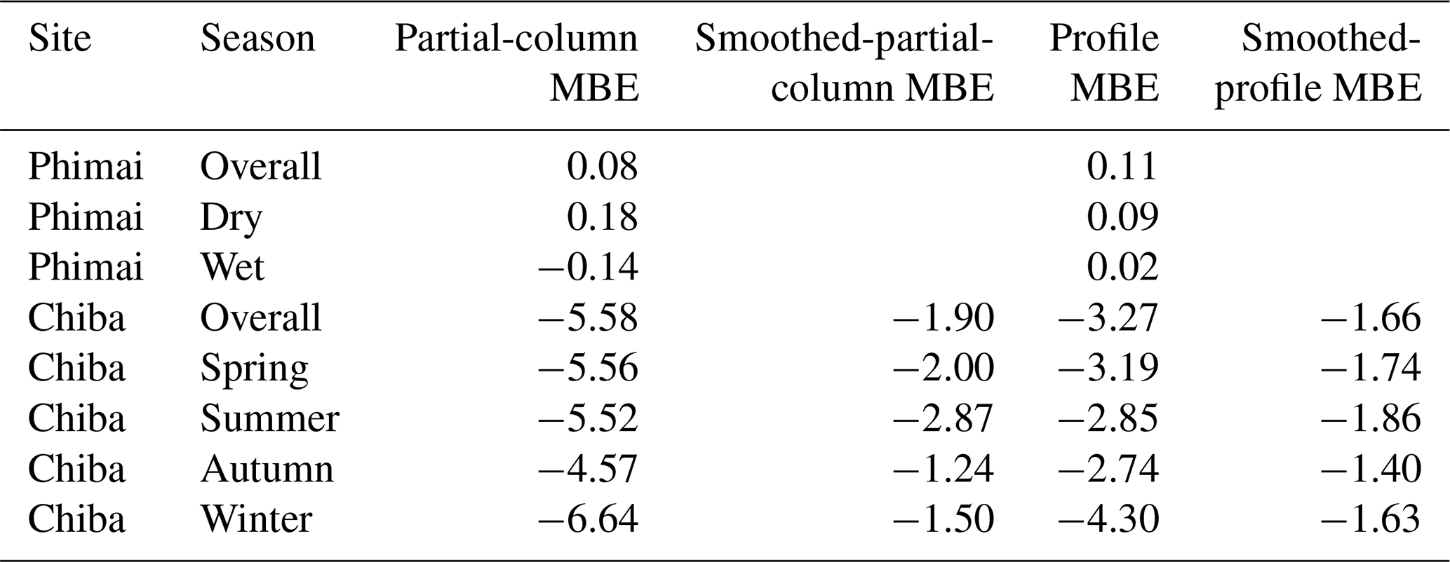
The modeled NO2 partial column at Phimai shows good agreement with observations made during the dry season. CHASER well reproduces the enhanced NO2 columns attributable to biomass burning within the standard deviation of the observations. The peak in the NO2 levels during March is consistent in both datasets. Although the seasonality does not agree in other months, the overall MBE is 8 × 10¹³ molecules cm−2 (Table 7). Above 500 m, the datasets show excellent agreement. The absolute mean differences in the 0–1 km layer are 0.22 ppbv, and the maximum difference of ∼ 1.9 ppbv is observed near the surface. Amid the biomass burning influence, the NO2 concentrations at Phimai are mostly < 1 ppbv. Thus, the results of comparisons demonstrate CHASER's good capabilities in regions characterized by low NO2 concentrations. Moreover, when NO2 concentrations are less than < 1 ppbv, the AK information seems less significant if the model can capture low-concentration scenarios.
Although the datasets are moderately correlated (R=0.59) at Chiba, the model largely underestimates the NO2 partial column with MBE of ∼ 5 × 10¹⁵ molecules cm−2. The model predicts almost constant NO2 profiles and columns throughout the year. Therefore, the respective seasonal biases are almost similar. The vertical gradient of the modeled NO2 profiles is also low, similarly to the HCHO profiles. The model resolution can be a potential cause for such significant underestimation. The AKs improved the partial column and profiles significantly, reducing the MBE by more than 50 %. However, the smoothed profiles and partial columns between the 0–2 km layer differ significantly from the simulations, suggesting that the a priori values strongly affect the smoothed profiles. Consequently, the smoothed NO2 profiles at Chiba (Fig. S7) are biased toward the a priori values, similarly to those of Phimai (Fig. S6). NO2 smoothed-profile sensitivity to a priori values might be attributable to our retrieval procedure. The a priori data are taken from the measured SCD and retrieved VCD values. As a result, the values are sensitive in the 0–2 km layer, similarly to the observations. Using a priori values other than those obtained from observations can affect such sensitivity. The smoothing sensitivity to a priori values is stronger for NO2 than HCHO. The NO2 profile gradient is higher than that of HCHO (Figs. 10 and 11), which means that, within 10 km (MAX-DOAS horizontal resolution), the NO2 mixing ratio and a priori variability (sources and sinks) are higher than those of HCHO, leading to a stronger a priori effect on the smoothed profiles.
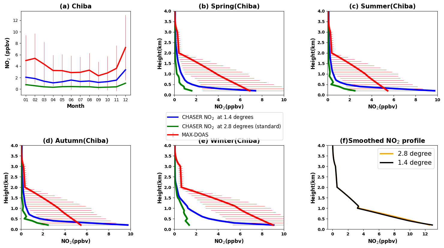
Figure 12(a) Seasonal variations in the NO2 mixing ratios in the 0–2 km layer at Chiba, as inferred from the MAX-DOAS observations (red) and two CHASER simulations at 2.8∘ (green) and 1.4∘ (blue) resolutions. The simulated NO2 profiles at 2.8∘ (green) and 1.4∘ (blue) resolutions during (b) spring, (c) summer, (d) autumn, and (e) winter are shown with the observed seasonal profiles at Chiba. Only data (both observed and simulated) for 2018 are plotted. The coincident time and date between the model and observations are selected only. The error bars in (a), (b), (c), (d), and (e) represent the 1σ standard deviation of mean values of the MAX-DOAS observations. (f) CHASER simulations at 2.8∘ (orange) and 1.4∘ (black) smoothed with MAX-DOAS AKs.
The mean NO2 mixing ratios in the 0–2 km layer in 2018, simulated at spatial resolutions of 2.8∘ × 2.8∘ (standard) and 1.4∘ × 1.4∘, are compared with observations at Chiba, as depicted in Fig. 12. The error bars are the 1σ standard deviation of the observations. Higher-resolution simulations reduced the overall MBE by 35 % (Table 8). NO2 concentrations at 1.4∘ are now within the variation range of the observations. The 1.4∘ simulation captured the NO2 seasonal variability better than at 2.8∘. Despite improved resolution, the model values are underestimated, with the highest MBE during the winter. According to Miyazaki et al. (2020), the seasonality in the anthropogenic emissions, primarily wintertime heating, is not well represented in the emission inventories, which could likely underestimate winter NO2 levels. The best agreement between the datasets is observed during summer and spring, with an MBE of ∼ 1 ppbv on a seasonal scale.
Table 8Comparison of the seasonal mean NO2profiles (0–2 km) among MAX-DOAS and CHASER simulations at 2.8 and 1.4∘ resolutions at Chiba. MBE (CHASER − MAX-DOAS) at 1.4 and 2.8∘ is the mean bias error at the respective resolutions. The MBE unit is parts per billion by volume (ppbv).

NO2 profiles at 2.8∘ and 1.4∘ resolution are shown in Fig. 12b–e. A strong effect of the increased resolution is observed below 500 m, reducing the negative bias by 70 % near the surface. Above 500 m, the effects of higher resolution are limited, with an MBE reduction of 12 % at 0.6–2 km. Although the near-surface NO2 concentrations at 1.4∘ resolution are overestimated, the values are within the standard deviation of the observations. At around 200 m, winter mean NO2 concentrations at 1.4∘ resolution are identical to the observations (∼ 9 ppbv) and the summer mean is overestimated. Moreover, the NO2 levels above 2 km are similar at both resolutions. The resolution effects on NO2 profiles vary with the location and season (Williams et al., 2017). For example, CHASER NO2 at 1.1∘ resolution improved the agreement with aircraft observations below 650 hPa significantly over the Denver metropolitan area (Sekiya et al., 2018), whereas, at Chiba, the 1.4∘ resolution improved the surface estimates. Consequently, the horizontal resolution is not the only reason for the model underestimation. Other factors such as the vertical resolution, uncertainties in emission inventories, and chemical kinetics can also affect the simulated NO2 estimates. Effects of the emission inventory are discussed in Sect. 3.3.4.
Figure 12f shows the smoothed NO2 profiles at both resolutions. Although the profile shapes are different, the smoothed profiles are almost identical, which demonstrates that smoothed-NO2-profile sensitivity to a priori choice is mostly independent of the model resolution.
3.3.3 Evaluation of CHASER HCHO in the IGP region
The IGP is the most fertile region in South Asia, accounts for approximately 50 % of the total agricultural production of India, and is one of the significant contributing regions to global greening based on the leaf area index (Sarmah et al., 2021). Moreover, the IGP is one of the regional HCHO hotspots in India (Chutia et al., 2019). The observed HCHO seasonality at Pantnagar is consistent with that reported by Mahajan et al. (2015) for the entire IGP region. Consequently, comparison with the HCHO retrievals in Pantnagar can assess the model capability in the IGP region. The spatial representativeness is a limitation for comparison between a point measurement and regional simulations. Thus, the results are interpreted qualitatively. Because of the availability of a dataset with continuous observations, only the comparison for 2017 is shown in Fig. 13.
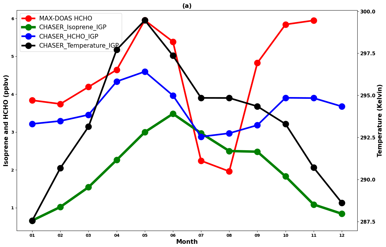
Figure 13Seasonal variations in the MAX-DOAS (red) and CHASER (blue) HCHO concentrations at Pantnagar and the IGP region, respectively, in 2017. Only the coincident dates between the observations and model are plotted. The CHASER-simulated isoprene and temperature seasonality are shown in green and black colors, respectively. Only the daytime simulated values were considered for the plot.
The modeled HCHO seasonal variations in the IGP region correlate well with the observations at Pantnagar (R ∼ 0.80). The enhancement in the HCHO concentrations during the spring and post-monsoon season is well reproduced by CHASER, which indicates that CHASER can capture HCHO variation in complex terrain region such as the IGP. Figure 13 also depicts the isoprene concentrations and temperature in the IGP region, in addition to the HCHO concentrations. Oxidization of precursor hydrocarbons and photochemical reactions are the most dominant sources of HCHO. Also, isoprene is the most abundant hydrocarbon in the atmosphere. The average ambient isoprene concentrations during July, August, and September in the IGP region are 1.4 ± 0.3 ppbv (Mishra and Sinha, 2020). Therefore, the CHASER isoprene concentration range of 1.5–2 ppbv during the monsoon season seems reasonable. The HCHO concentrations in the IGP region reach a peak during the spring and post-monsoon seasons. A strong correlation between HCHO, isoprene, and temperature variation (R ∼ 0.90) during the first half of the year indicates that the change in biogenic emissions strongly drives the HCHO seasonal modulation. The observed enhancement in the HCHO levels during spring at Pantnagar is related to biomass burning. The biomass burning events are primarily concentrated in the northwest IGP region (Kumar and Sinha, 2021), where the site is located. On a regional scale, the biomass burning effects are expected to become smeared. Thus, the strong effect of the biogenic emission on the regional HCHO modulation is reasonable. HCHO modulation differs from isoprene and temperature during the post-monsoon period, suggesting a greater role of biomass burning and anthropogenic emissions. Consequently, the physical processes driving the HCHO seasonality in the IGP region are well reflected in the CHASER simulations.
3.3.4 Effects of the model resolution and emission inventories on results
Effects of the spatial resolution on the evaluation results are assessed by comparing the results of CHASER simulations at 2.8 and 1.4∘ resolutions with the surface observations, as shown in Fig. 14. Only the simulated surface HCHO and NO2 concentrations during 2017 are shown only. The statistics are provided in Table 9. For the Pantnagar site, only the simulations are presented. At Phimai, the HCHO simulations differ by 3 %. The standard simulation shows better agreement with the observations. The higher MBE at 1.4∘ occurred mostly because of the model overestimation during the wet season. The NO2 mixing ratios at the two resolutions differ by 9 %. The MBEs for both trace gases at Phimai are less than 1 ppbv. Thus, the HCHO and NO2 standard simulations at 2.8∘ can be regarded as reasonable for regions characterized by low NO2 levels (< 1 ppbv). At Chiba, surface NO2 and HCHO mixing ratios at 1.4∘ resolution differ by 61 % and 19 %, respectively. The NO2 MBE at 1.4∘ resolution improved significantly, indicating a strong effect of the model resolution. However, discussion in Sect. 3.2.2 showed limited resolution-based improvement in the overall profile. Results for MBE in the HCHO mixing ratios at 1.4∘ mostly improved during summer. The wintertime HCHO estimates at both resolutions are similar. In contrast to Chiba and Phimai, differences in the HCHO simulations (30 %) at Pantnagar are greater than those of NO2 (3 %). The effect of model resolution varying with location and season was also reported by Sekiya et al. (2018). Compared to the other two sites, differences in the NO2 simulations at Chiba are larger. This finding is consistent with the results by Williams et al. (2017), who found larger differences with changing model resolution over urban areas.
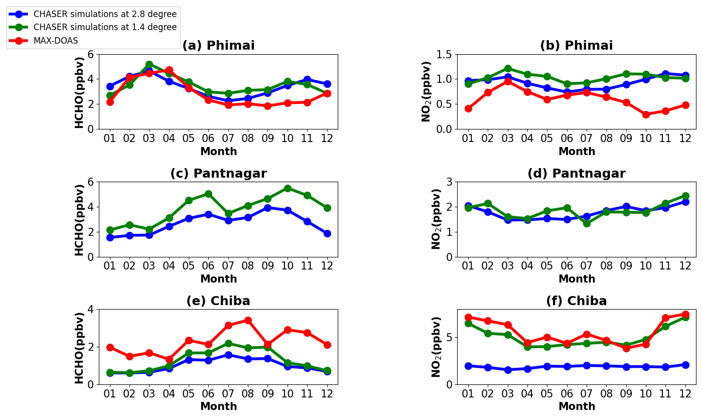
Figure 14Seasonal variation in the surface HCHO and NO2 mixing ratios at (a, b) Phimai, (c, d) Pantnagar, and (e, f) Chiba simulated at spatial resolutions of 2.8∘ × 2.8∘ (blue) and 1.4∘ × 1.4∘ (green). Coincident MAX-DOAS NO2 and HCHO VMRs in the 0–1 km layer at Phimai and Chiba are plotted in red. Observations at Pantnagar are discarded. Only the datasets for 2017 are plotted.
Table 9The comparison between the observations and simulations at 2.8 and 1.4∘ spatial resolutions. The MBE is the mean bias error. The unit of MBE is parts per billion by volume (ppbv).
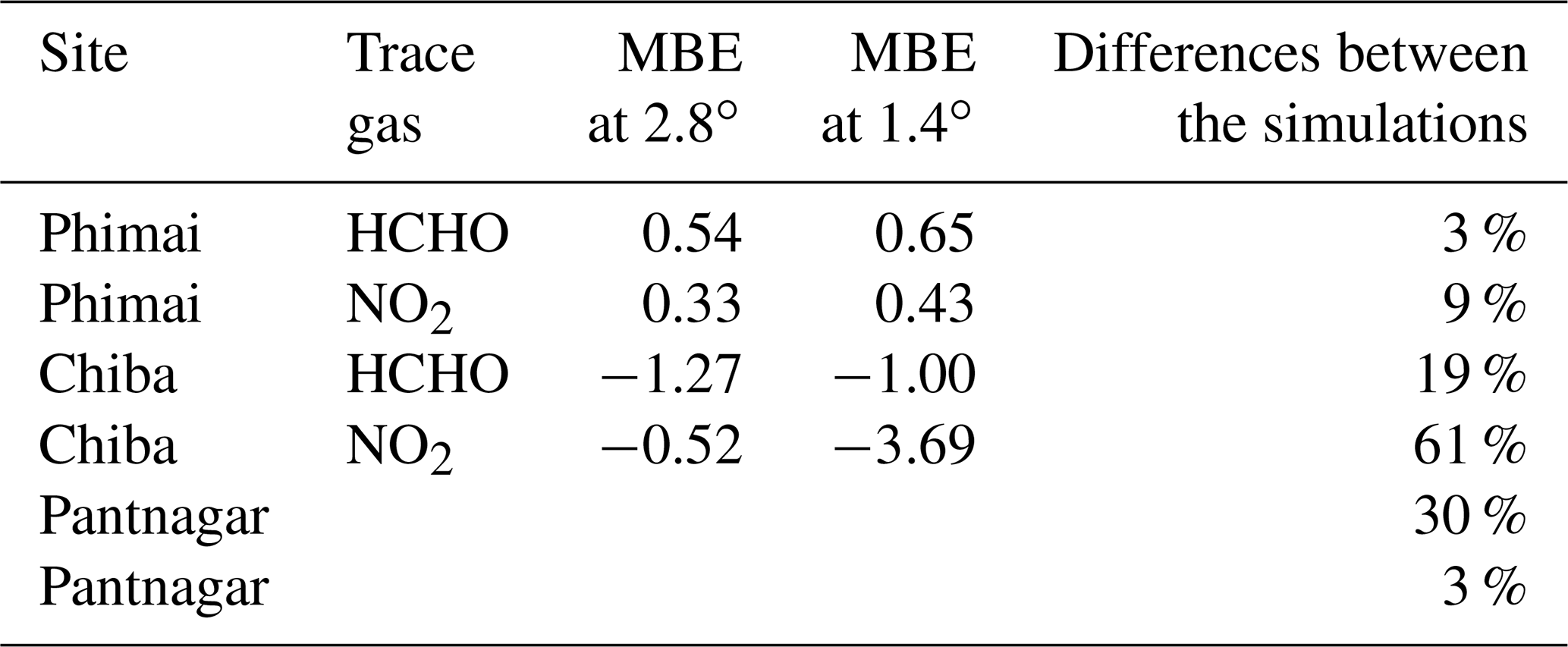
Although the NOx estimates for the low-NO2 regions seem reasonable, global NOx emissions have changed since 2008 (i.e., HTAP 2008 emissions used for this study). A recent study by Miyazaki et al. (2020) reported changes in global NOx emissions from 2005 to 2018. They found a continuous 30 % increase in NOx emissions in India since 2005. REAS v3 (Regional Emission inventory in ASia version 3) inventory estimated a 23 % increase in NOx emissions in India between 2010–2015, and power plants were the most significant contributor. Many power plants are clustered along the IGP region (Nair et al., 2007). Thus, the current simulation settings are likely to underestimate the NO2 mixing ratios and columns in the IGP region. Figure S8 presents comparison of CHASER and OMI NO2 columns for 2017 over the IGP region. Although the modeled columns are biased by 32 % on the lower side, the spatial correlation between the datasets is high (r=0.78). CHASER values lie within the range of variation in the observations. Although underestimated, NO2 estimates in the IGP based on the current inventory are still reasonable. Sekiya et al. (2018) used higher model resolution and an updated emission inventory (HTAP 2010 for simulations in 2014) and reported ∼ 30 % lower MBE over India. However, the RMSE values of both studies are comparable.
NOx emissions in Japan have shown continuous decline since the execution of pollution control policies in 1970 (Ohara et al., 2007). Irie et al. (2021) reported a declining trend in NO2 levels in Chiba since 2012, echoing results obtained by Miyazaki et al. (2020) throughout Japan. The bias between the CHASER and OMI NO2 column over Japan is non-significant (Fig. S8 and Table S3). Thus, an updated inventory will not substantially affect the comparison results at the Chiba site. NOx emissions increased considerably in Southeast Asia. CHASER NO2 estimates for Thailand based on the HTAP 2008 inventory are biased by 45 % on the lower side compared to OMI (Fig. S8). However, Phimai being a rural site, the NOx levels are expected to be low. Changes in biomass burning NOx estimates are likely to affect the model estimates. Because the NO2 levels at Phimai are mostly less than 1 ppbv, the effect of an updated inventory on the comparison results is expected to be minimal.
CHASER HCHO columns over Japan, the IGP region, and Thailand are negatively biased by 60 %, 36 %, and 32 %, respectively, compared to OMI observations, with r values of 0.5–0.7 (Fig. S8). Surl et al. (2018) reported spatial correlation of ∼ 0.5 between GEOS-Chem and OMI over the IGP region. Anthropogenic VOC emissions in India and other Asian cities have increased since 2005, whereas a negative trend has been observed over Japan (Bauwens et al., 2022). The REAS inventory estimated a 5 % increase in NMVOCS in India since 2005. Moreover, anthropogenic emission contributes strongly to the HCHO abundances in the IGP region (Kumar and Sinha, 2021). Thus, an updated anthropogenic VOC emission inventory is likely to improve the model HCHO estimates in the study regions. However, the formation pathway of HCHO from isoprene emissions is a non-linear function of NOx chemistry. Consequently, the effects of NOx emissions changes on the overall HCHO simulations cannot be assessed based on current analyses explained herein.
3.4 Contribution estimates
3.4.1 Contribution from biomass burning to the HCHO and NO2 abundances at Phimai
Good agreement between the datasets in the 0–1 km layer at Phimai can quantify biomass burning contributions to the HCHO and NO2 concentrations. Figure 15 presents results of simulations L1_HCHO, L1_opt, and L1_NO2. The simulation settings are presented in Table 3. For better readability, the switched-off emissions criterion is described in the legends of Fig. 15. The plots present mean mixing ratios in the 0–1 km layer. Biomass burning contributes ∼ 10 % to the HCHO concentrations at Phimai during the dry season. However, based on the observations, a greater effect of biomass burning is expected. During the wet season, the MAX-DOAS and CHASER HCHO surface mixing ratios are ∼ 2 and ∼ 4 ppbv, respectively (Fig. 10), indicating overestimation of the biogenic emissions in CHASER. Figure 15b shows the HCHO concentration obtained from simulation L1_opt and MAX-DOAS observations in 2017. In the L1_opt simulation setting, the biomass burning emissions are switched off; the biogenic emissions are optimized to reproduce results analogous to those obtained from observations during the wet season. In the absence of biomass burning, the surface HCHO concentrations at Phimai would be ∼ 2 ppbv, indicating a biomass burning contribution of ∼ 20 %–50 % during the dry season. The observed interseason difference in the HCHO concentration at Phimai is ∼ 60 %. Consequently, the revised biomass burning contribution estimate is more reasonable. Pyrogenic emissions contributions to the NO2 concentrations at Phimai are ∼ 10 % during the dry season (Fig. 15c). Because the NO2 concentrations are low at Phimai, the simulation results obtained for March, when the influence of biomass burning is highest, are used to derive a better contribution estimate. In the absence of biomass burning, the NO2 concentration during March would be about 0.84 ppbv (Fig. 15d), indicating a contribution as high as 35 % to the NO2 concentrations at Phimai.
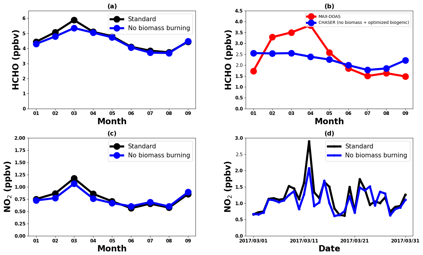
Figure 15(a) Seasonal variations in the HCHO concentrations in the 0–1 km layer at Phimai, as obtained from the standard and L1_HCHO simulations. Pyrogenic emissions of VOCs are switched off in L1_HCHO. (b) The HCHO seasonal variation in Phimai in 2017, as obtained from the MAX-DOAS observations (red) and L1_opt simulations. The pyrogenic VOC emissions are switched off and the biogenic emissions are reduced by 50 % in L1_opt. Only the coincident dates between the observation and the simulations are shown. (c) Seasonal variations in the NO2 surface concentrations at Phimai in 2017, as obtained from the standard and L1_NO2 simulations. (d) Standard and L1_NO2 simulation outputs of the daily mean NO2 surface concentrations during March 2017 (the date format is year/month/day). The pyrogenic NO2 emissions were switched off in the L1_NO2 simulation. Only the daytime values from 09:00–15:00 LT are used to calculate the seasonal mean.
3.4.2 Contribution of soil NOx emissions at Phimai
Because soil NOx emissions are included in CHASER simulations, the NO2 contributions from soil emissions are quantified. Figure 16 presents the monthly mean surface NO2 concentrations at Phimai in 2017, simulated including (standard) and switching off (L1_NO2) the soil NOx emissions. The NO2 concentrations between 09:00 and 12:00 LT were used to calculate the monthly mean concentrations. Soil emissions contribute ∼ 20 % of the overall NO2 concentrations at Phimai, with higher contributions during the wet season. The highest soil contribution of about 25 % occurs in July.
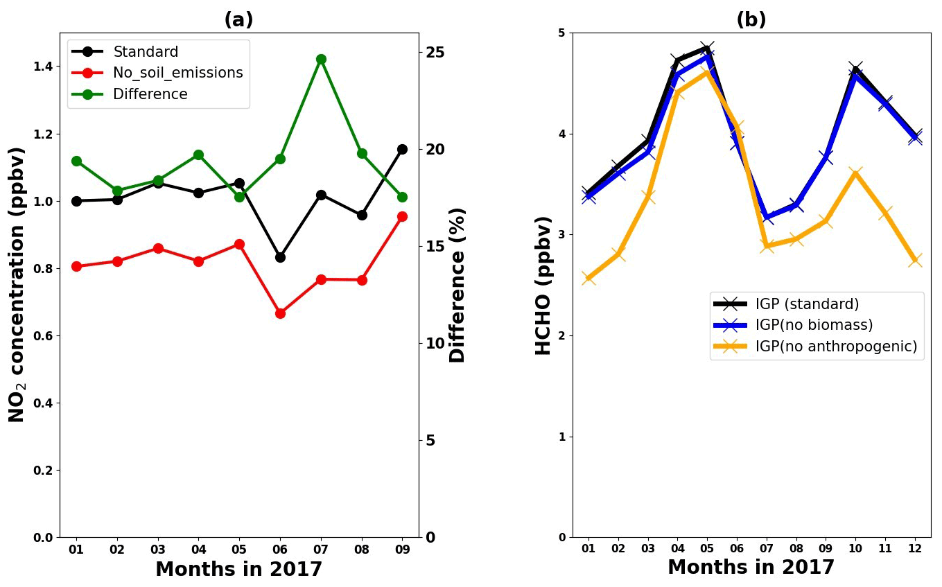
Figure 16(a) Monthly mean NO2 concentrations at Phimai were estimated from the standard (black) and L1_NO2 (red) simulations. The soil NOx emissions are switched off in the LI_NO2 simulation. The green line represents the percentage difference between the two simulations. (b) Seasonal variations in the HCHO concentrations in the IGP region, obtained from the standard, L1_HCHO (pyrogenic VOC emissions switched off), and L2 simulations (anthropogenic VOC emissions switched off). The simulations for 2017 are shown and analyzed. Daytime values from 09:00–12:00 and 09:00–15:00 LT were selected for Phimai and the IGP, respectively.
3.4.3 Contribution from pyrogenic and anthropogenic emissions to the HCHO abundances in the IGP region
Figure 16b presents the standard, L1_HCHO (pyrogenic VOC emissions switched off), and L2 (anthropogenic VOC emissions switched off) HCHO simulations in the IGP region. According to L1_HCHO simulation results, effects of biomass burning emissions on the regional HCHO modulation are small (∼ 12 %). The HCHO concentrations in India have biogenic, anthropogenic, and pyrogenic VOC sources. However, biogenic VOCs are the primary driver of the overall HCHO variation (Surl et al., 2018). Consequently, two reasons might be responsible for the small effects of pyrogenic emissions on HCHO concentrations: (1) overestimation of the biogenic emission or underestimation of pyrogenic emissions in the model and (2) stronger effects of anthropogenic VOC emissions than of pyrogenic VOCs. The L2 simulations show that anthropogenic emissions contribute up to 30 % of the HCHO concentration in the IGP region, with a maximum contributed during the post-monsoon season, which coincides with the lower isoprene concentration (i.e., biogenic emissions) and temperature (Fig. 14). Moreover, Kumar and Sinha (2021) reported high acetaldehyde concentrations from anthropogenic emissions in the IGP region throughout the year. Consequently, anthropogenic emissions are likely to be a significant driver of HCHO concentrations in the IGP region after biogenic emissions.
Using the JM2 algorithm, NO2 and HCHO concentrations and profiles were retrieved from MAX-DOAS observations at three A-SKY sites during January 2017–December 2018. The retrieved products were used to evaluate the global chemistry transport model CHASER simulations at the three sites. At all three locations, the seasonal variation in both trace gases was consistent throughout the investigated period. At Phimai and Pantnagar, biomass burning led to enhanced HCHO and NO2 concentrations, respectively, during the dry season and spring and post-monsoon season. At Chiba, the HCHO variation was consistent with the temperature-led seasonal changes in biogenic emissions. The changes in the dry-season HCHO and NO2 levels at Phimai during 2015–2018 were consistent with the number of fire events.
The RFN values were biased toward a particular regime when the standard transition range 1 < RFN < 2 (Duncan et al., 2010) was used. The parameterization of Souri et al. (2020) provides a better estimate of the transition region. The classification results of the revised transition region at Phimai and Pantnagar contradicted the results based on the standard transition range. However, they were more reasonable. Such a method based on observations is therefore influenced by measurement constraints. More observational evidence must be accumulated to standardize this method. Overall, the results further indicated that the standard transition region is not valid globally.
Despite the use of an old NOx emission inventory, the simulated NO2 and HCHO spatial distributions agreed reasonably well with those from satellite observations. The modeled regional NO2 column estimates were within the 2σ variability range of OMI NO2 retrievals. Although the negative bias in HCHO comparison was higher than that of NO2, the model demonstrated good capabilities for simulating the HCHO seasonal variation in different regions.
CHASER showed good capabilities at Phimai, characterized as a VOC-rich and low-NO2 (< 1 ppbv) region. In both seasons, the observed and modeled profiles (HCHO and NO2) agreed within the 1σ standard deviation of the measurements, despite general overestimation of the model. Furthermore, both wet-season HCHO profiles were almost identical in the 0.5–4 km layer in both datasets.
CHASER demonstrated limited performance at Chiba. NO2 at higher resolution (i.e.,1.4∘) mainly improved the surface estimates, reducing the overall MBE in the 0–2 km layer by 35 %. Finer resolution would improve the HCHO estimates in Chiba by 10 %; however, it still is underestimated. Sensitivity studies for the Phimai site estimated biomass burning contributions to HCHO and NO2 concentrations of up to ∼ 50 % and ∼ 35 %, respectively. On average, 20 % of the NO2 level originates from soil NOx emissions, increasing to 25 % in July. Anthropogenic emissions (contribution of up to 30 %) have a larger impact on VOC variation in the IGP region than biomass burning, which is consistent with earlier reports in the literature.
The CHASER and JM2 source codes are not available publicly. Kengo Sudo (kengo@nagoya-u.jp) is the contact person for readers and researchers interested in the CHASER model. In addition, Hitoshi Irie (hitoshi.irie@chiba-u.jp) will answer queries related to the JM2 codes.
The MAX-DOAS data used in the study are publicly accessible on the A-SKY network website (http://atmos3.cr.chiba-u.jp/a-sky/data.html, last access: 26 September 2022; Irie, 2021). Upon request, the corresponding author can provide the CHASER simulations and MAX-DOAS averaging-kernel data.
The supplement related to this article is available online at: https://doi.org/10.5194/acp-22-12559-2022-supplement.
HMSH conceptualized the study, conducted the model simulations, analyzed the observational and simulation data, and drafted the manuscript. AMF helped with the data processing. HI developed the JM2 code and maintained the A-SKY network. KS developed the CHASER model and supervised the study. MN is the principal investigator of the Pantnagar site. AD and MN shared their experience to explain the results. HI, KS, AD, MN, and AMF commented and provided feedback on the final results and manuscript.
The contact author has declared that none of the authors has any competing interests.
Publisher’s note: Copernicus Publications remains neutral with regard to jurisdictional claims in published maps and institutional affiliations.
The CHASER model simulations are partly performed with the supercomputer (NEC SX-Aurora TSUBASA) at the National Institute for Environmental Studies (NIES), Tsukuba, Japan. The authors are grateful to the OMI and TROPOMI data providers. Support from the ISRO-ATCTM project for the Pantnagar site is also acknowledged.
This research has been supported by the Ministry of the Environment, Government of Japan (Global Environmental Research Fund (grant nos. S-12 and S-20)), and the Japan Society for the Promotion of Science (grant nos. JP20H04320, JP19H05669, and JP19H04235).
This paper was edited by Andreas Richter and reviewed by two anonymous referees.
Amnuaylojaroen, T., Inkom, J., Janta, R., and Surapipith, V.: Long range transport of southeast asian PM2.5 pollution to northern Thailand during high biomass burning episodes, Sustainability, 12, 10049, https://doi.org/10.3390/su122310049, 2020.
Arlander, D., Brüning, D., Schmidt, U., and Ehhalt, D.: The tropospheric distribution of formaldehyde during TROPOZ II, J. Atmos. Chem., 22, 251–269, https://doi.org/10.1007/BF00696637, 1995.
Bauwens, M., Verreyken, B., Stavrakou, T., Müller, J. F., and De Smedt, I.: Spaceborne evidence for significant anthropogenic VOC trends in Asian cities over 2005–2019, Environ. Res. Lett., 17, 015008, https://doi.org/10.1088/1748-9326/ac46eb, 2022.
Biswas, M. S. and Mahajan, A. S.: Year-long Concurrent MAX-DOAS Observations of Nitrogen Dioxide and Formaldehyde at Pune: Understanding Diurnal and Seasonal Variation Drivers, Aerosol Air Qual. Res., 21, 200524, https://doi.org/10.4209/aaqr.200524, 2021.
Biswas, M. S., Ghude, S. D., Gurnale, D., Prabhakaran, T., and Mahajan, A. S.: Simultaneous Observations of Nitrogen Dioxide, Formaldehyde and Ozone in the Indo-Gangetic Plain, Aerosol Air Qual. Res., 19, 1749–1764, https://doi.org/10.4209/aaqr.2018.12.0484, 2019.
Boeke, N. L., Marshall, J. D., Alvarez, S., Chance, K. V., Fried, A., Kurosu, T. P., Rappengluck, B., Richter, D., Walega, J., and Weibring, P.: Formaldehyde columns from the Ozone Monitoring Instrument: Urban versus background levels and evaluation using aircraft data and a global model, J. Geophys. Res., 116, D05303, https://doi.org/10.1029/2010JD014870, 2011.
Boersma, K. F., Eskes, H. J., Dirksen, R. J., van der A, R. J., Veefkind, J. P., Stammes, P., Huijnen, V., Kleipool, Q. L., Sneep, M., Claas, J., Leitão, J., Richter, A., Zhou, Y., and Brunner, D.: An improved tropospheric NO2 column retrieval algorithm for the Ozone Monitoring Instrument, Atmos. Meas. Tech., 4, 1905–1928, https://doi.org/10.5194/amt-4-1905-2011, 2011.
Bogumil, K., Orphal, J., Homann, T., Voigt, S., Spietz, P., Fleischmann, O., Vogel, A., Hartmann, M., Kromminga, H., and Bovensmann, H.: Measurements of molecular absorption spectra with the SCIAMACHY pre-flight model: instrument characterization and reference data for atmospheric remote-sensing in the 230–2380 nm region, J. Photocho. Photobio. A, 157, 167–184, https://doi.org/10.1016/S1010-6030(03)00062-5, 2003.
Bond, D. W., Zhang, R., Tie, X., Brasseur, G., Huffines, G., Orville, R. E., and Boccippio, D. J.: NOx production by lightning over the continental United States, J. Geophys. Res., 106, 27701–27710, https://doi.org/10.1029/2000JD000191, 2001.
Burkert, J., Andrés-Hernández, M. D., Stöbener, D., Burrows, J. P., Weissenmayer, M., and Kraus, A.: Peroxy radical and related trace gas measurements in the boundary layer above the Atlantic Ocean, J. Geophys. Res., 106, 5457–5477, https://doi.org/10.1029/2000JD900613, 2001.
Cárdenas, L., Rondón, A., Johansson, C., and Sanhueza, E.: Effects of soil moisture, temperature, and inorganic nitrogen on nitric oxide emissions from acidic tropical savannah soils, J. Geophys. Res., 98, 14783–14790, https://doi.org/10.1029/93JD01020, 1993.
Chan, K. L., Wiegner, M., van Geffen, J., De Smedt, I., Alberti, C., Cheng, Z., Ye, S., and Wenig, M.: MAX-DOAS measurements of tropospheric NO2 and HCHO in Munich and the comparison to OMI and TROPOMI satellite observations, Atmos. Meas. Tech., 13, 4499–4520, https://doi.org/10.5194/amt-13-4499-2020, 2020.
Chance, K. V. and Spurr, R. J. D.: Ring effect studies: Rayleigh scattering, including molecular parameters for rotational Raman scattering: and the Fraunhofer spectrum, Appl. Opt., 36, 5224–5230, https://doi.org/10.1364/AO.36.005224, 1997.
Chutia, L., Ojha, N., Girach, I. A., Sahu, L. K., Alvarado, L. M. A., Burrows, J. P., Pathak., P., and Bhuyan, P. K.: Distribution of volatile organic compounds over Indian subcontinent during winter: WRF-chem simulation versus observations, Environ. Pollut., 252, 256–269, https://doi.org/10.1016/j.envpol.2019.05.097, 2019.
Clémer, K., Van Roozendael, M., Fayt, C., Hendrick, F., Hermans, C., Pinardi, G., Spurr, R., Wang, P., and De Mazière, M.: Multiple wavelength retrieval of tropospheric aerosol optical properties from MAXDOAS measurements in Beijing, Atmos. Meas. Tech., 3, 863–878, https://doi.org/10.5194/amt-3-863-2010, 2010.
Colella, P. and Woodward, P. R.: The piecewise parabolic method (PPM) for gas-dynamical simulations, J. Comput. Phys., 54, 174–201, https://doi.org/10.1016/0021-9991(84)90143-8, 1984.
Crutzen, P. J.: The influence of nitrogen oxides on the atmospheric ozone content, Q. J. Roy. Meteor. Soc., 96, 320–325, https://doi.org/10.1002/qj.49709640815, 1970.
De Smedt, I., Pinardi, G., Vigouroux, C., Compernolle, S., Bais, A., Benavent, N., Boersma, F., Chan, K.-L., Donner, S., Eichmann, K.-U., Hedelt, P., Hendrick, F., Irie, H., Kumar, V., Lambert, J.-C., Langerock, B., Lerot, C., Liu, C., Loyola, D., Piters, A., Richter, A., Rivera Cárdenas, C., Romahn, F., Ryan, R. G., Sinha, V., Theys, N., Vlietinck, J., Wagner, T., Wang, T., Yu, H., and Van Roozendael, M.: Comparative assessment of TROPOMI and OMI formaldehyde observations and validation against MAX-DOAS network column measurements, Atmos. Chem. Phys., 21, 12561–12593, https://doi.org/10.5194/acp-21-12561-2021, 2021.
Duncan, B. N., Yoshida, Y., Olson, J. R., Sillman, S., Martin, R. V., Lamsal, L., Hu, Y., Pickering, K. E., retscher, C., Allen, D. J., and Crawford, J. H.: Application of OMI observations to a space-based indicator of NOx and VOC controls on surface ozone formation, Atmos. Environ., 44, 2213–2223, https://doi.org/10.1016/j.atmosenv.2010.03.010, 2010.
Emori, S., Nozawa, T., Numaguti, A., and Uno, I.: Importance of cumulus parameterization for precipitation simulation over East Asia in June, J. Meteorol. Soc. Jpn., 79, 939–947, https://doi.org/10.2151/jmsj.79.939, 2001.
Fleischmann, O. C., Hartmann, M., Burrows, J. P., and Orphal, J.: New ultraviolet absorption cross-sections of BrO at atmospheric temperatures measured by time-windowing Fourier transform spectroscopy, J. Photocho. Photobio. A, 168, 117–132, https://doi.org/10.1016/j.jphotochem.2004.03.026, 2004.
Franco, B., Hendrick, F., Van Roozendael, M., Müller, J.-F., Stavrakou, T., Marais, E. A., Bovy, B., Bader, W., Fayt, C., Hermans, C., Lejeune, B., Pinardi, G., Servais, C., and Mahieu, E.: Retrievals of formaldehyde from ground-based FTIR and MAX-DOAS observations at the Jungfraujoch station and comparisons with GEOS-Chem and IMAGES model simulations, Atmos. Meas. Tech., 8, 1733–1756, https://doi.org/10.5194/amt-8-1733-2015, 2015.
Frieß, U., Monks, P. S., Remedios, J. J., Rozanov, A., Sinreich, R., Wagner, T., and Platt, U.: MAX-DOAS O4 measurements: A new technique to derive information on atmospheric aerosols: 2. Modeling studies, J. Geophys. Res., 111, D14203, https://doi.org/10.1029/2005JD006618, 2006.
Frieß, U., Klein Baltink, H., Beirle, S., Clémer, K., Hendrick, F., Henzing, B., Irie, H., de Leeuw, G., Li, A., Moerman, M. M., van Roozendael, M., Shaiganfar, R., Wagner, T., Wang, Y., Xie, P., Yilmaz, S., and Zieger, P.: Intercomparison of aerosol extinction profiles retrieved from MAX-DOAS measurements, Atmos. Meas. Tech., 9, 3205–3222, https://doi.org/10.5194/amt-9-3205-2016, 2016.
Fu, T. M., Jacob, D. J., Wittrock, F., Burrows, J. P., Vrekoussis, M., and Henze, D. K.: Global budgets of atmospheric glyoxal and methylglyoxal, and implications for formation of secondary organic aerosols, J. Geophys. Res., 113, D15303, https://doi.org/10.1029/2007JD009505, 2008.
Giles, D. M., Holben, B. N., Tripathi, S. N, Eck, T. F., Newcomb, W. W., Slutsker, I., Dickerson, R. R., Thompson, A. M., Mattoo, S., Wang, S.‐H., Singh, R. P., Sinyuk, A., and Schafer, J. S.: Aerosol properties over the Indo‐Gangetic Plain: A mesoscale perspective from the TIGERZ experiment, J. Geophys. Res., 116, D18203, https://doi.org/10.1029/2011JD015809, 2011.
Fukushima, A., Kanamori, H., and Matsumoto, J.: Regionality of long-term trends and interannual variation of seasonal precipitation over India, Prog. Earth Planet. Sci., 6, 1–20, https://doi.org/10.1186/s40645-019-0255-4, 2019.
Hak, C., Pundt, I., Trick, S., Kern, C., Platt, U., Dommen, J., Ordóñez, C., Prévôt, A. S. H., Junkermann, W., Astorga-Lloréns, C., Larsen, B. R., Mellqvist, J., Strandberg, A., Yu, Y., Galle, B., Kleffmann, J., Lörzer, J. C., Braathen, G. O., and Volkamer, R.: Intercomparison of four different in-situ techniques for ambient formaldehyde measurements in urban air, Atmos. Chem. Phys., 5, 2881–2900, https://doi.org/10.5194/acp-5-2881-2005, 2005.
Hall, S. J., Matson, P. A., and Roth, P. M.: NOx emissions from soil: implications for air quality modeling in agricultural regions, Annu. Rev. Energy Environ., 21, 311–346, https://doi.org/10.1146/annurev.energy.21.1.311, 1996.
Halla, J. D., Wagner, T., Beirle, S., Brook, J. R., Hayden, K. L., O'Brien, J. M., Ng, A., Majonis, D., Wenig, M. O., and McLaren, R.: Determination of tropospheric vertical columns of NO2 and aerosol optical properties in a rural setting using MAX-DOAS, Atmos. Chem. Phys., 11, 12475–12498, https://doi.org/10.5194/acp-11-12475-2011, 2011.
Hendrick, F., Müller, J.-F., Clémer, K., Wang, P., De Mazière, M., Fayt, C., Gielen, C., Hermans, C., Ma, J. Z., Pinardi, G., Stavrakou, T., Vlemmix, T., and Van Roozendael, M.: Four years of ground-based MAX-DOAS observations of HONO and NO2 in the Beijing area, Atmos. Chem. Phys., 14, 765–781, https://doi.org/10.5194/acp-14-765-2014, 2014.
Hermans, C., Vandaele, A., Fally, S., Carleer, M., Colin, R., Coquart, B., Jenouvrier, A., and Merienne, M.-F.: Absorption cross-section of the collision-induced bands of oxygen from the UV to the NIR, in: Weakly interacting molecular pairs: unconventional absorbers of radiation in the atmosphere, NATO Science Book series, Springer, 193–202, https://doi.org/10.1007/978-94-010-0025-3_16, 2003.
Hönninger, G., von Friedeburg, C., and Platt, U.: Multi axis differential optical absorption spectroscopy (MAX-DOAS), Atmos. Chem. Phys., 4, 231–254, https://doi.org/10.5194/acp-4-231-2004, 2004.
Hoque, H. M. S., Irie, H., and Damiani, A.: First MAX-DOAS Observations of Formaldehyde and Glyoxal in Phimai, Thailand, J. Geophys. Res., 123, 9957–9975, https://doi.org/10.1029/2018JD028480, 2018a.
Hoque, H. M. S., Irie, H., Damiani, A., Rawat, P., and Naja, M.: First simultaneous observations of formaldehyde and glyoxal by MAX-DOAS in the Indo-Gangetic Plain region, Sola, 14, 159–164, https://doi.org/10.2151/sola.2018-028, 2018b.
Houweling, S., Dentener, F., and Lelieveld, J.: The impact of nonmethane hydrocarbon compounds on tropospheric photochemistry, J. Geophys. Res., 103, 10673–10696, https://doi.org/10.1029/97JD03582, 1998.
Huber, D. E., Steiner, A. L., and Kort, E. A.: Daily Cropland Soil NOx Emissions Identified by TROPOMI and SMAP, Geophys. Res. Lett., 47, e2020GL089949, https://doi.org/10.1029/2020GL089949, 2020.
Irie, H.: MAX-DOAS data, International air quality and sky research remote sensing (A-SKY) network [data set], http://atmos3.cr.chiba-u.jp/a-sky/data.html (last access: 26 September 2022), 2021.
Irie, H., Kanaya, Y., Akimoto, H., Iwabuchi, H., Shimizu, A., and Aoki, K.: First retrieval of tropospheric aerosol profiles using MAX-DOAS and comparison with lidar and sky radiometer measurements, Atmos. Chem. Phys., 8, 341–350, https://doi.org/10.5194/acp-8-341-2008, 2008a.
Irie, H., Kanaya, Y., Akimoto, H., Tanimoto, H., Wang, Z., Gleason, J. F., and Bucsela, E. J.: Validation of OMI tropospheric NO2 column data using MAX-DOAS measurements deep inside the North China Plain in June 2006: Mount Tai Experiment 2006, Atmos. Chem. Phys., 8, 6577–6586, https://doi.org/10.5194/acp-8-6577-2008, 2008b.
Irie, H., Kanaya, Y., Akimoto, H., Iwabuchi, H., Shimizu, A., and Aoki, K.: Dual-wavelength aerosol vertical profile measurements by MAX-DOAS at Tsukuba, Japan, Atmos. Chem. Phys., 9, 2741–2749, https://doi.org/10.5194/acp-9-2741-2009, 2009.
Irie, H., Takashima, H., Kanaya, Y., Boersma, K. F., Gast, L., Wittrock, F., Brunner, D., Zhou, Y., and Van Roozendael, M.: Eight-component retrievals from ground-based MAX-DOAS observations, Atmos. Meas. Tech., 4, 1027–1044, https://doi.org/10.5194/amt-4-1027-2011, 2011.
Irie, H., Nakayama, T., Shimizu, A., Yamazaki, A., Nagai, T., Uchiyama, A., Zaizen, Y., Kagamitani, S., and Matsumi, Y.: Evaluation of MAX-DOAS aerosol retrievals by coincident observations using CRDS, lidar, and sky radiometer inTsukuba, Japan, Atmos. Meas. Tech., 8, 2775–2788, https://doi.org/10.5194/amt-8-2775-2015, 2015.
Irie, H., Muto, T., Itahashi, S., Kurokawa, J., and Uno, I.: Turnaround of tropospheric nitrogen dioxide pollution trends in China, Japan, and South Korea, Sola, 12, 170–174, https://doi.org/10.2151/sola.2016-035, 2016.
Irie, H., Yonekawa, D., Damiani, A., Hoque, H. M. S., Sudo, K., and Itahashi, S.: Continuous multi-component MAX-DOAS observations for the planetary boundary layer ozone variation analysis at Chiba and Tsukuba, Japan, from 2013 to 2019, Prog. Earth Planet. Sci., 8, 1–11, https://doi.org/10.1186/s40645-021-00424-9, 2021.
Ito, A. and Inatomi, M.: Use of a process-based model for assessing the methane budgets of global terrestrial ecosystems and evaluation of uncertainty, Biogeosciences, 9, 759–773, https://doi.org/10.5194/bg-9-759-2012, 2012.
Iwabuchi, H.: Efficient Monte Carlo methods for radiative transfer modeling, J. Atmos. Sci., 63, 2324–2339, https://doi.org/10.1175/JAS3755.1, 2006.
Jang, M. and Kamens, R. M.: Characterization of secondary aerosol from the photooxidation of toluene in the presence of NOx and 1-propene, Environ. Sci. Technol., 35, 3626–3639, https://doi.org/10.1021/es010676+, 2001.
Jenkin, M. E., Young, J. C., and Rickard, A. R.: The MCM v3.3.1 degradation scheme for isoprene, Atmos. Chem. Phys., 15, 11433–11459, https://doi.org/10.5194/acp-15-11433-2015, 2015.
Jin, X. and Holloway, T.: Spatial and temporal variability of ozone sensitivity over China observed from the Ozone Monitoring Instrument, J. Geophys. Res., 120, 7229–7246, https://doi.org/10.1002/2015JD023250, 2015.
Jin, X., Fiore, A. M., Murray, L. T., Valin, L. C., Lamsal, L. N., Duncan, B., Boersma, K. F., De Smedt, I., Abad, G. G., Chance, K., and Tonnesen, G.: Evaluating a space-based indicator of surface ozone-NOx-VOC sensitivity over midlatitude source regions and application to decadal trends. J. Geophys. Res., 122, 10439–10461, https://doi.org/10.1002/2017JD026720, 2017.
Joshi, H., Manish, N., Singh, K. P., Kumar, R., Bhardwaj, P., Babu, S. S., Satheesh, S. K., Moorthy, K. K., and Chandola, H. C.: Investigations of aerosol black carbon from a semi-urban site in the Indo-Gangetic Plain region, Atmos. Environ., 125, 346–359, https://doi.org/10.1016/j.atmosenv.2015.04.007, 2016.
Kanakidou, M., Seinfeld, J. H., Pandis, S. N., Barnes, I., Dentener, F. J., Facchini, M. C., Van Dingenen, R., Ervens, B., Nenes, A., Nielsen, C. J., Swietlicki, E., Putaud, J. P., Balkanski, Y., Fuzzi, S., Horth, J., Moortgat, G. K., Winterhalter, R., Myhre, C. E. L., Tsigaridis, K., Vignati, E., Stephanou, E. G., and Wilson, J.: Organic aerosol and global climate modelling: a review, Atmos. Chem. Phys., 5, 1053–1123, https://doi.org/10.5194/acp-5-1053-2005, 2005.
Kanaya, Y., Irie, H., Takashima, H., Iwabuchi, H., Akimoto, H., Sudo, K., Gu, M., Chong, J., Kim, Y. J., Lee, H., Li, A., Si, F., Xu, J., Xie, P.-H., Liu, W.-Q., Dzhola, A., Postylyakov, O., Ivanov, V., Grechko, E., Terpugova, S., and Panchenko, M.: Long-term MAX-DOAS network observations of NO2 in Russia and Asia (MADRAS) during the period 2007–2012: instrumentation, elucidation of climatology, and comparisons with OMI satellite observations and global model simulations, Atmos. Chem. Phys., 14, 7909–7927, https://doi.org/10.5194/acp-14-7909-2014, 2014.
Kannari, A., Tonooka, Y., Baba, T., and Murano, K.: Development of multiple-species 1 km × 1 km resolution hourly basis emissions inventory for Japan, Atmos. Environ., 41, 3428–3439, https://doi.org/10.1016/j.atmosenv.2006.12.015, 2007.
Khodmanee, S. and Amnuaylojaroen, T.: Impact of Biomass Burning on Ozone, Carbon Monoxide, and Nitrogen Dioxide in Northern Thailand, Front. Enviorn. Sci., 9, 27, https://doi.org/10.3389/fenvs.2021.641877, 2021.
Kreher, K., Van Roozendael, M., Hendrick, F., Apituley, A., Dimitropoulou, E., Frieß, U., Richter, A., Wagner, T., Lampel, J., Abuhassan, N., Ang, L., Anguas, M., Bais, A., Benavent, N., Bösch, T., Bognar, K., Borovski, A., Bruchkouski, I., Cede, A., Chan, K. L., Donner, S., Drosoglou, T., Fayt, C., Finkenzeller, H., Garcia-Nieto, D., Gielen, C., Gómez-Martín, L., Hao, N., Henzing, B., Herman, J. R., Hermans, C., Hoque, S., Irie, H., Jin, J., Johnston, P., Khayyam Butt, J., Khokhar, F., Koenig, T. K., Kuhn, J., Kumar, V., Liu, C., Ma, J., Merlaud, A., Mishra, A. K., Müller, M., Navarro-Comas, M., Ostendorf, M., Pazmino, A., Peters, E., Pinardi, G., Pinharanda, M., Piters, A., Platt, U., Postylyakov, O., Prados-Roman, C., Puentedura, O., Querel, R., Saiz-Lopez, A., Schönhardt, A., Schreier, S. F., Seyler, A., Sinha, V., Spinei, E., Strong, K., Tack, F., Tian, X., Tiefengraber, M., Tirpitz, J.-L., van Gent, J., Volkamer, R., Vrekoussis, M., Wang, S., Wang, Z., Wenig, M., Wittrock, F., Xie, P. H., Xu, J., Yela, M., Zhang, C., and Zhao, X.: Intercomparison of NO2, O4, O3 and HCHO slant column measurements by MAX-DOAS and zenith-sky UV–visible spectrometers during CINDI-2, Atmos. Meas. Tech., 13, 2169–2208, https://doi.org/10.5194/amt-13-2169-2020, 2020.
Kumar, V. and Sinha, V.: Season-wise analyses of VOCs, hydroxyl radicals and ozone formation chemistry over north-west India reveal isoprene and acetaldehyde as the most potent ozone precursors throughout the year, Chemosphere, 283, 131184, https://doi.org/10.1016/j.chemosphere.2021.131184, 2021.
Kumar, V., Beirle, S., Dörner, S., Mishra, A. K., Donner, S., Wang, Y., Sinha, V., and Wagner, T.: Long-term MAX-DOAS measurements of NO2, HCHO, and aerosols and evaluation of corresponding satellite data products over Mohali in the Indo-Gangetic Plain, Atmos. Chem. Phys., 20, 14183–14235, https://doi.org/10.5194/acp-20-14183-2020, 2020.
Kurucz, R. L., Furenlid, I., Brault, J., and Testerman, L.: Solar flux atlas from 296 to 1300 nm: National Solar Observatory Atlas No. 1, Sunspot, New Mexico, 1984.
Lee, M., Heikes, B. G., Jacob, D. J., Sachse, G., and Anderson, B.: Hydrogen peroxide, organic hydroperoxide, and formaldehyde as primary pollutants from biomass burning, J. Geophys. Res., 102, 1301–1309, https://doi.org/10.1029/96JD01709, 1997.
Lelieveld, J., Berresheim, H., Borrmann, S., Crutzen, P. J., Dentener, F. J., Fischer, H., Feichter, J., Flatau, J., Heland, J., Holzinger, R., Korrmann, R., Lawrence, M. G., Levin, Z., Markowicz, K. M., Mihalopoulos, N., Minikin, A., Ramanathan, V., De Reues, M., Roelofs, J., Scheeren, H. A., Sciare, J., Schlager, H., Schultz, M., Seigmund, P., Stephanou, E. G., Steil, B., Traub, M., Warneke,C., Williams, J., and Ziereis, H.: Global air pollution crossroads over the Mediterranean, Science, 298, 794–799, https://doi.org/10.1126/science.1075457, 2002.
Levelt, P. F., Van Den Oord, G. H. J, Dobber, M. R., Malkki, A., Visser, H., De Vries, J., Stammes, P., Lundell, J. O. V., and Saari, H.: The ozone monitoring instrument, IEEE T. Geosci. Remote, 44, 1093–1101, https://doi.org/10.1109/TGRS.2006.872333, 2006.
Lin, S.-J. and Rood, R. B.: Multidimensional flux-form semi-Lagrangian transport schemes, Mon. Weather Rev., 124, 2046–2070, https://doi.org/10.1175/1520-0493(1996)124<2046:MFFSLT>2.0.CO;2, 1996.
Lu, X., Zhang, L., Liu, X., Gao, M., Zhao, Y., and Shao, J.: Lower tropospheric ozone over India and its linkage to the South Asian monsoon, Atmos. Chem. Phys., 18, 3101–3118, https://doi.org/10.5194/acp-18-3101-2018, 2018.
Ma, J. Z., Beirle, S., Jin, J. L., Shaiganfar, R., Yan, P., and Wagner, T.: Tropospheric NO2 vertical column densities over Beijing: results of the first three years of ground-based MAX-DOAS measurements (2008–2011) and satellite validation, Atmos. Chem. Phys., 13, 1547–1567, https://doi.org/10.5194/acp-13-1547-2013, 2013.
Mahajan, A. S., De Smedt, I., Biswas, M. S., Ghude, S., Fadnavis, S., Roy, C., and van Roozendael, M.: Inter-annual variations in satellite observations of nitrogen dioxide and formaldehyde over India, Atmos. Environ., 116, 194–201, https://doi.org/10.1016/j.atmosenv.2015.06.004, 2015.
Martin, R. V., Fiore, A. M., and Van Donkelaar, A.: Space-based diagnosis of surface ozone sensitivity to anthropogenic emissions, Geophys. Res. Lett., 31, L06120, https://doi.org/10.1029/2004GL019416, 2004.
Meller, R. and Moortgat, G. K.: Temperature dependence of the absorption cross sections of formaldehyde between 223 and 323 K in the wavelength range 225–375 nm, J. Geophys. Res., 105, 7089–7101, https://doi.org/10.1029/1999JD901074, 2000.
Mellor, G. L. and Yamada, T.: A hierarchy of turbulence closure models for planetary boundary layers, J. Atmos. Sci., 31, 1791–1806, https://doi.org/10.1175/1520-0469(1974)031<1791:AHOTCM>2.0.CO;2, 1974.
Mishra, A. K. and Sinha, V.: Emission drivers and variability of ambient isoprene, formaldehyde and acetaldehyde in north-west India during monsoon season, Environ. Pollut., 267, 115538, https://doi.org/10.1016/j.envpol.2020.115538, 2020.
Miyazaki, K., Eskes, H. J., and Sudo, K.: Global NOx emission estimates derived from an assimilation of OMI tropospheric NO2 columns, Atmos. Chem. Phys., 12, 2263–2288, https://doi.org/10.5194/acp-12-2263-2012, 2012.
Miyazaki, K., Eskes, H., Sudo, K., Boersma, K. F., Bowman, K., and Kanaya, Y.: Decadal changes in global surface NOx emissions from multi-constituent satellite data assimilation, Atmos. Chem. Phys., 17, 807–837, https://doi.org/10.5194/acp-17-807-2017, 2017.
Miyazaki, K., Bowman, K., Sekiya, T., Eskes, H., Boersma, F., Worden, H., Livesey, N., Payne, V. H., Sudo, K., Kanaya, Y., Takigawa, M., and Ogochi, K.: Updated tropospheric chemistry reanalysis and emission estimates, TCR-2, for 2005–2018, Earth Syst. Sci. Data, 12, 2223–2259, https://doi.org/10.5194/essd-12-2223-2020, 2020.
Morino, Y., Ohara, T., Yokouchi, Y., and Ooki, A.: Comprehensive source apportionment of volatile organic compounds using observational data, two receptor models, and an emission inventory in Tokyo metropolitan area, J. Geophys. Res., 116, D02311, https://doi.org/10.1029/2010JD014762, 2011.
Nair, V. S., Moorthy, K. K., Alappattu, D. P., Kunhikrishnan, P. K., George, S., Nair, P. R., Babu, S. S., Abish, A., Satheesh, S. K., Tripathi, S. N., Niranjan, K., Madhavan, B. L., Srikant, V., Dutt, C. B. S., Badarinath, K. V. S., and Reddy, R. R.: Wintertime aerosol characteristics over the Indo-Gangetic Plain (IGP): Impacts of local boundary layer processes and long-range transport, J. Geophys. Res., 112, D13205, https://doi.org/10.1029/2006JD008099, 2007.
Ohara, T., Akimoto, H., Kurokawa, J., Horii, N., Yamaji, K., Yan, X., and Hayasaka, T.: An Asian emission inventory of anthropogenic emission sources for the period 1980–2020, Atmos. Chem. Phys., 7, 4419–4444, https://doi.org/10.5194/acp-7-4419-2007, 2007.
Platt, U. and Stutz, J.: Differential Optical Absorption Spectroscopy, Physics of Earth and Space Environment, Springer, Berlin, Heidelberg, https://doi.org/10.1007/978-3-540-75776-4, 2008.
Price, C. and Rind, D.: A simple lightning parameterization for calculating global lightning distributions, J. Geophys. Res., 97, 9919–9933, https://doi.org/10.1029/92JD00719, 1992.
Rodgers, C. D.: Inverse methods for atmospheric sounding: theory and practice, World scientific, Singapore, https://doi.org/10.1142/3171, 2000.
Roscoe, H. K., Van Roozendael, M., Fayt, C., du Piesanie, A., Abuhassan, N., Adams, C., Akrami, M., Cede, A., Chong, J., Clémer, K., Friess, U., Gil Ojeda, M., Goutail, F., Graves, R., Griesfeller, A., Grossmann, K., Hemerijckx, G., Hendrick, F., Herman, J., Hermans, C., Irie, H., Johnston, P. V., Kanaya, Y., Kreher, K., Leigh, R., Merlaud, A., Mount, G. H., Navarro, M., Oetjen, H., Pazmino, A., Perez-Camacho, M., Peters, E., Pinardi, G., Puentedura, O., Richter, A., Schönhardt, A., Shaiganfar, R., Spinei, E., Strong, K., Takashima, H., Vlemmix, T., Vrekoussis, M., Wagner, T., Wittrock, F., Yela, M., Yilmaz, S., Boersma, F., Hains, J., Kroon, M., Piters, A., and Kim, Y. J.: Intercomparison of slant column measurements of NO2 and O4 by MAX-DOAS and zenith-sky UV and visible spectrometers, Atmos. Meas. Tech., 3, 1629–1646, https://doi.org/10.5194/amt-3-1629-2010, 2010.
Ryan, R. G., Rhodes, S., Tully, M., and Schofield, R.: Surface ozone exceedances in Melbourne, Australia are shown to be under NOx control, as demonstrated using formaldehyde: NO2 and glyoxal: formaldehyde ratios, Sci. Total Environ., 749, 141460, https://doi.org/10.1016/j.scitotenv.2020.141460, 2020.
Sadavarte, P. and Venkataraman, C.: Trends in multi-pollutant emissions from a technology-linked inventory for India: I. Industry and transport sectors, Atmos. Environ., 99, 353–364, https://doi.org/10.1016/j.atmosenv.2014.09.081, 2014.
Sarmah, S., Singha, M., Wang, J., Dong, J., Burman, P. K. D., Goswami, S., Ge. Y., Ilyas, S., and Niu, S.: Mismatches between vegetation greening and primary productivity trends in South Asia–A satellite evidence. Int. J. Appl. Eath Obs., 104, 102561, https://doi.org/10.1016/j.jag.2021.102561, 2021.
Schindlbacher, A., Zechmeister-Boltenstern, S., and Butterbach-Bahl, K.: Effects of soil moisture and temperature on NO, NO2, and N2O emissions from European forest soils, J. Geophys. Res., 109, D17302, https://doi.org/10.1029/2004JD004590, 2004.
Schroeder, J. R., Crawford, J. H., Fried, A., Walega, J., Weinheimer, A., Wisthaler, A., Muller, M., Mikovinu, T., Chen, G., and Shook, M.: New insights into the column CH2O NO2 ratio as an indicator of near-surface ozone sensitivity, J. Geophys. Res., 122, 8885–8907, https://doi.org/10.1002/2017JD026781, 2017.
Seco, R., Penuelas, J., and Filella, I.: Short-chain oxygenated VOCs: Emission and uptake by plants and atmospheric sources, sinks, and concentrations, Atmos. Environ., 41, 2477–2499, https://doi.org/10.1016/j.atmosenv.2006.11.029, 2007.
Seinfeld, J. H. and Pandis, S. N.: Atmospheric chemistry and physics: from air pollution to climate change, John Wiley & Sons, New York, ISBN 9780471720188, 1998.
Sekiya, T. and Sudo, K.: Roles of transport and chemistry processes in global ozone change on interannual and multidecadal time scales, J. Geophys. Res., 119, 4903–4921, https://doi.org/10.1002/2013JD020838, 2014.
Sekiya, T., Miyazaki, K., Ogochi, K., Sudo, K., and Takigawa, M.: Global high-resolution simulations of tropospheric nitrogen dioxide using CHASER V4.0, Geosci. Model Dev., 11, 959–988, https://doi.org/10.5194/gmd-11-959-2018, 2018.
Sharma, S., Goel, A., Gupta, D., Kumar, A., Mishra, A., Kundu, S., Chatani, S., and Klimont, Z.: Emission inventory of non-methane volatile organic compounds from anthropogenic sources in India, Atmos. Environ., 102, 209–219, https://doi.org/10.1016/j.atmosenv.2014.11.070, 2015.
Sindelarova, K., Markova, J., Simpson, D., Huszar, P., Karlicky, J., Darras, S., and Granier, C.: High-resolution biogenic global emission inventory for the time period 2000–2019 for air quality modelling, Earth Syst. Sci. Data, 14, 251–270, https://doi.org/10.5194/essd-14-251-2022, 2022.
Singh, H., Salas, L., Chatfield, R., Czech, E., Fried, A., Walega, J., Evans, M. J., Field, B. D., Jacob, D. J., Blake, D., Heikes, B., Talbolt, R., Sachse, G., Crawford, J. H., Avery, M. A., Sandholm, S., and Fuelberg, H.: Analysis of the atmospheric distribution, sources, and sinks of oxygenated volatile organic chemicals based on measurements over the Pacific during TRACE-P, J. Geophys. Res., 109, D15S07, https://doi.org/10.1029/2003JD003883, 2004.
Sinreich, R., Frieß, U., Wagner, T., and Platt, U.: Multi axis differential optical absorption spectroscopy (MAX-DOAS) of gas and aerosol distributions, Faraday Discuss., 130, 153–164, https://doi.org/10.1039/B419274P, 2005.
Solomon, S., Portmann, R., Sanders, R., Daniel, J., Madsen, W., Bartram, B., and Dutton, E.: On the role of nitrogen dioxide in the absorption of solar radiation, J. Geophys. Res., 104, 12047–12058, https://doi.org/10.1029/1999JD900035, 1999.
Souri, A. H., Nowlan, C. R., Wolfe, G. M., Lamsal, L. N., Miller, C. E. C., Abad, G. G., Janz, S., Fried, A., Blake, D. R., Weinheimer, A. J., Diskin, G. S., Liu, X., and Chance, K.: Revisiting the effectiveness of HCHO/NO2 ratios for inferring ozone sensitivity to its precursors using high resolution airborne remote sensing observations in a high ozone episode during the KORUS-AQ campaign, Atmos. Environ., 224, 117341, https://doi.org/10.1016/j.atmosenv.2020.117341, 2020.
Sudo, K. and Akimoto, H.: Global source attribution of tropospheric ozone: Long-range transport from various source regions, J. Geophys. Res., 112, D12302, https://doi.org/10.1029/2006JD007992, 2007.
Sudo, K., Takahashi, M., Kurokawa, J., and Akimoto, H.: CHASER: A global chemical model of the troposphere 1. Model description, J. Geophys. Res., 107, 4339, https://doi.org/10.1029/2001JD001113, 2002.
Surl, L., Palmer, P. I., and González Abad, G.: Which processes drive observed variations of HCHO columns over India?, Atmos. Chem. Phys., 18, 4549–4566, https://doi.org/10.5194/acp-18-4549-2018, 2018.
Takemura, T., Nozawa, T., Emori, S., Nakajima, T. Y., and Nakajima, T.: Simulation of climate response to aerosol direct and indirect effects with aerosol transport-radiation model, J. Geophys. Res., 110, D02202, https://doi.org/10.1029/2004JD005029, 2005.
Takemura, T., Egashira, M., Matsuzawa, K., Ichijo, H., O'ishi, R., and Abe-Ouchi, A.: A simulation of the global distribution and radiative forcing of soil dust aerosols at the Last Glacial Maximum, Atmos. Chem. Phys., 9, 3061–3073, https://doi.org/10.5194/acp-9-3061-2009, 2009.
Tonnesen, G. S. and Dennis, R. L.: Analysis of radical propagation efficiency to assess ozone sensitivity to hydrocarbons and NOx: 1. Local indicators of instantaneous odd oxygen production sensitivity, J. Geophys. Res., 105, 9213–9225, https://doi.org/10.1029/1999JD900371, 2000.
Vandaele, A. C., Hermans, C., Simon, P. C., Van Roozendael, M., Guilmot, J. M., Carleer, M., and Colin, R. : Fourier transform measurement of NO2 absorption cross-section in the visible range at room temperature, J. Atmos. Chem., 25, 289–305, https://doi.org/10.1007/BF00053797, 1996.
Vandaele, A. C., Fayt, C., Hendrick, F., Hermans, C., Humbled, F., Roozendael, M. V., Gil, M., Navarro, M., Puentedura, O., Yela, M., Braathen, G., Stebel, K., Tornkvist, K., Jhonston, P., Kreher, K., Goutail, F., Mieville, F., Pommereau, J. P., Khaikine, S., Richter, A., Oetjen, H., Wittrock, F., Bugarski, S., Friess, U., Pfeilsticker, K., Sinreich, R., Wagner, T., Corlett, G., and Leigh, R.: An intercomparison campaign of ground-based UV-visible measurements of NO2, BrO, and OClO slant columns Methods of analysis and results for NO2, J. Geophys. Res., 110, D08305, https://doi.org/10.1029/2004JD005423, 2005.
Vigouroux, C., Hendrick, F., Stavrakou, T., Dils, B., De Smedt, I., Hermans, C., Merlaud, A., Scolas, F., Senten, C., Vanhaelewyn, G., Fally, S., Carleer, M., Metzger, J.-M., Müller, J.-F., Van Roozendael, M., and De Mazière, M.: Ground-based FTIR and MAX-DOAS observations of formaldehyde at Réunion Island and comparisons with satellite and model data, Atmos. Chem. Phys., 9, 9523–9544, https://doi.org/10.5194/acp-9-9523-2009, 2009.
Wagner, T., Dix, B. V., Friedeburg, C. V., Frieß, U., Sanghavi, S., Sinreich, R., and Platt, U.: MAX-DOAS O4 measurements: A new technique to derive information on atmospheric aerosols – Principles and information content, J. Geophys. Res., 109, D2205, https://doi.org/10.1029/2004JD004904, 2004.
Wagner, T., Burrows, J. P., Deutschmann, T., Dix, B., von Friedeburg, C., Frieß, U., Hendrick, F., Heue, K.-P., Irie, H., Iwabuchi, H., Kanaya, Y., Keller, J., McLinden, C. A., Oetjen, H., Palazzi, E., Petritoli, A., Platt, U., Postylyakov, O., Pukite, J., Richter, A., van Roozendael, M., Rozanov, A., Rozanov, V., Sinreich, R., Sanghavi, S., and Wittrock, F.: Comparison of box-air-mass-factors and radiances for Multiple-Axis Differential Optical Absorption Spectroscopy (MAX-DOAS) geometries calculated from different UV/visible radiative transfer models, Atmos. Chem. Phys., 7, 1809–1833, https://doi.org/10.5194/acp-7-1809-2007, 2007.
Wang, T., Hendrick, F., Wang, P., Tang, G., Clémer, K., Yu, H., Fayt, C., Hermans, C., Gielen, C., Müller, J.-F., Pinardi, G., Theys, N., Brenot, H., and Van Roozendael, M.: Evaluation of tropospheric SO2 retrieved from MAX-DOAS measurements in Xianghe, China, Atmos. Chem. Phys., 14, 11149–11164, https://doi.org/10.5194/acp-14-11149-2014, 2014.
Weller, R., Schrems, O., Boddenberg, A., Gäb, S., and Gautrois, M.: Meridional distribution of hydroperoxides and formaldehyde in the marine boundary layer of the Atlantic (48∘ N–35∘ S) measured during the Albatross campaign, J. Geophys. Res., 105, 14401–14412, https://doi.org/10.1029/1999JD901145, 2000.
Wesely, M.: Parameterization of surface resistances to gaseous dry deposition in regional-scale numerical models, Atmos. Environ., 41, 52–63, https://doi.org/10.1016/j.atmosenv.2007.10.058, 1989.
Williams, J. E., Boersma, K. F., Le Sager, P., and Verstraeten, W. W.: The high-resolution version of TM5-MP for optimized satellite retrievals: description and validation, Geosci. Model Dev., 10, 721–750, https://doi.org/10.5194/gmd-10-721-2017, 2017.
Wittrock, F., Oetjen, H., Richter, A., Fietkau, S., Medeke, T., Rozanov, A., and Burrows, J. P.: MAX-DOAS measurements of atmospheric trace gases in Ny-Ålesund – Radiative transfer studies and their application, Atmos. Chem. Phys., 4, 955–966, https://doi.org/10.5194/acp-4-955-2004, 2004.
Woo, J.-H., Kim, Y., Kim, H.-K., Choi, K.-C., Eum, J.-H., Lee, J.-B., Lim, J.-H., Kim, J., and Seong, M.: Development of the CREATE inventory in support of integrated climate and air quality modeling for Asia, Sustainability, 12, 7930, https://doi.org/10.3390/su12197930, 2020.
Zara, M., Boersma, K. F., De Smedt, I., Richter, A., Peters, E., van Geffen, J. H. G. M., Beirle, S., Wagner, T., Van Roozendael, M., Marchenko, S., Lamsal, L. N., and Eskes, H. J.: Improved slant column density retrieval of nitrogen dioxide and formaldehyde for OMI and GOME-2A from QA4ECV: intercomparison, uncertainty characterisation, and trends, Atmos. Meas. Tech., 11, 4033–4058, https://doi.org/10.5194/amt-11-4033-2018, 2018.
Zarzana, K. J., Min, K., Washenfelder, R. A., Kaiser, J., Krawiec-Thayer, M., Peischl, J., Neuman, J. A., Nowak, J. B., Wagner, N. L., Dubè, W. P., Clair, J. M. S. C., Wolfe, G. M., Hanisco, F., Keutsch, F. N., Ryerson, T. B., and Brown, S. S.: Emissions of glyoxal and other carbonyl compounds from agricultural biomass burning plumes sampled by aircraft, Environ. Sci. Technol., 51, 11761–11770, https://doi.org/10.1021/acs.est.7b03517, 2017.
Zhang, R., Tie, X., and Bond, D. W.: Impacts of anthropogenic and natural NOx sources over the US on tropospheric chemistry, P. Natl. Acad. Sci. Sci., 100, 1505–1509, https://doi.org/10.1073/pnas.252763799, 2003.
Zheng, X., Wang, M., Wang, Y., Shen, R., Gou, J., Li, J., Jin, J., and Li, L.: Impacts of soil moisture on nitrous oxide emission from croplands: a case study on the rice-based agro-ecosystem in Southeast China, Chemosphere, 2, 207–224, https://doi.org/10.1016/S1465-9972(99)00056-2, 2000.