The impacts of secondary ice production on microphysics and dynamics in tropical convection

Secondary ice production (SIP) is an important physical phenomenon that results in an increase in the ice particle concentration and can therefore have a significant impact on the evolution of clouds. In this study, idealized simulations of a mesoscale convective system (MCS) were conducted using a high-resolution (250 m horizontal grid spacing) mesoscale model and a detailed bulk microphysics scheme in order to examine the impacts of SIP on the microphysics and dynamics of a simulated tropical MCS. The simulations were compared to airborne in situ and remote sensing observations collected during the “High Altitude Ice Crystals – High Ice Water Content” (HAIC-HIWC) field campaign in 2015. It was found that the observed high ice number concentration can only be simulated by models that include SIP processes. The inclusion of SIP processes in the microphysics scheme is crucial for the production and maintenance of the high ice water content observed in tropical convection. It was shown that SIP can enhance the strength of the existing convective updrafts and result in the initiation of new updrafts above the melting layer. Agreement between the simulations and observations highlights the impacts of SIP on the maintenance of tropical MCSs in nature and the importance of including SIP parameterizations in models.

1 Introduction

Secondary ice production (SIP) is recognized as a fundamental cloud microphysical process (e.g., Cantrell and Heymsfield, 2005; Field et al., 2017). Production of secondary ice involves processes that require the presence of pre-existing ice particles. SIP is different from primary ice production (PIP), which commences by the nucleation of ice either homogeneously in strongly supercooled droplets or heterogeneously on the surface of ice-nucleating particles (INPs) (e.g., Kanji et al., 2017).

The first in situ observations of SIP go back to the early 1960s (e.g., Murgatroyd and Garrod, 1960; Koenig, 1963, 1965). Multiyear in situ measurements have shown that SIP is an very common phenomenon, and it occurs in different types of clouds from polar regions to the tropics; these findings are based on recent SIP studies including Lloyd et al. (2015), Lawson et al. (2015, 2017), Lasher-Trapp et al. (2016), Keppas et al. (2017), Mignani et al. (2019), Korolev and Leisner (2020), Li et al. (2021), Luke et al. (2021), and many others.

The primary effect of SIP is the enhancement of the ice particle concentration that, depending on environmental conditions, may exceed the concentration of PIP ice particles by several orders of magnitude (e.g., Hobbs and Rangno, 1985; Ladino et al., 2017). Such an enhancement of the ice particle concentration may have a significant effect on the phase composition, cloud dynamics, precipitation rate, and cloud radiative properties, impacting the energy balance and hydrological cycle on regional and global scales.

At present, seven mechanisms are recognized as sources of secondary ice in clouds. These include the fragmentation of freezing droplets (hereafter FFD; e.g., Kleinheins et al., 2021), rime splintering (i.e., the Hallett–Mossop process, hereafter HM; e.g., Hallett and Mossop, 1974), fragmentation due to ice–ice collisions (e.g., Vardiman 1978; Takahashi et al. 1995), ice fragmentation due to thermal shock (e.g., Dye and Hobbs, 1968), fragmentation of sublimating ice (Oraltay and Hallett, 1989), activation of INPs in transient supersaturation around freezing drops (e.g., Prabhakaran et al., 2020), and break-up of freezing water drops on impact with ice particles (James et al., 2021). A detailed description of the first six SIP mechanisms and the status of associated laboratory studies are discussed in the review by Korolev and Leisner (2020). It was found that HM and FFD are the most experimentally studied SIP mechanisms, as well as the mechanisms for which production rates of secondary ice have been quantified. However, a detailed analysis of previous experiments by Korolev and Leisner (2020) revealed a large diversity of the ice production rates, which led to the conclusion that these SIP processes need to be studied further. The other four mechanisms have a limited number of laboratory experiments, and they cover only a fraction of environmental conditions (e.g., fragmentation during ice collisions and fragmentation of sublimating ice) or only demonstrate the general feasibility of SIP mechanisms (e.g., fragmentation due to thermal shock and activation of INPs in transient supersaturation around freezing drops). All of the above-mentioned information led Korolev and Leisner (2020) to the conclusion that the relative contributions of each of the six SIP mechanisms in the enhancement of ice concentrations remain uncertain.

Over the last few years, there have been many new efforts based on systematic studies of the effect of SIP on cloud microphysics with the help of cloud simulations (e.g., Phillips et al., 2017, 2018; Sullivan et al., 2018; Hoarau et al., 2018; Fu et al., 2019; Sotiropoulou et al., 2020, 2021; Dedekind et al., 2021; Hawker et al., 2021; Huang et al., 2021, 2022; and others). Most of these modelling efforts have been focused on matching simulated moments of particle size distributions (PSDs) with those observed in situ. In many ways, the implementation of SIP in numerical models has been hindered by the lack of consensus on the parameterizations of SIP mechanisms.

One of the main objectives of this work is to identify and simulate the occurrence of high ice water content (IWC) associated with the enhancement of ice particle concentrations from SIP processes. Cloud environments with high IWC (> 1 g m⁻³) pose a hazard for civil aviation and may result in engine power loss, stall, or damage (e.g., Lawson et al., 1998; Mason et al., 2006; Mason and Grzych, 2011). The phenomenon of high IWC has been well documented from in situ observations in tropical mesoscale convective systems (MCSs) (e.g., Heymsfield and Palmer, 1986; Lawson et al., 1998; Gayet et al., 2012; Fridlind et al., 2015; Leroy et al., 2017; Strapp et al., 2021). Several previous modelling studies using different cloud microphysical parameterizations have attempted to reproduce high IWCs. Ackerman et al. (2015) used a 1D model to explore microphysics in tropical MCSs. Simulations performed with 3D models (Franklin et al., 2016; Stanford et al., 2017; Qu et al., 2018) pointed to inaccuracies in the estimation of cloud PSD, IWC, and ice category compared with the observations. Huang et al. (2021) conducted high-resolution simulations of tropical convection and found significant overestimates of radar reflectivity and underestimates of total ice crystal concentration (N_i). Adding SIP in high-resolution simulations, Huang et al. (2022) found a significant improvement in simulated N_i compared with the in situ observations.

In most of the previous numerical studies investigating SIP, the microphysics schemes used were based on the traditional approach of representing ice-phase hydrometeors by partitioning them into various predefined categories (e.g., pristine ice, snow, and graupel) with prescribed physical properties. This approach has several inherent limitations and problems, including a limited range of ice properties (e.g., bulk density) that can be represented, inconsistent physical processes applied to the categories, and the need to parameterize conversion between categories – an artificial process which can not be constrained from observations and is purely ad hoc. To address this problem, Morrison and Milbrandt (2015) proposed a new approach and developed a new microphysics parameterization – the Predicted Particle Properties (P3) scheme – whereby all ice-phase hydrometeors are represented by a single “free” ice category whose physical properties evolve continuously. While flexible in this regard, one limitation of the original P3 scheme was that it could not represent more than one population of ice particles (with different bulk properties) at a given time and grid location. Thus, the scheme was generalized to allow for a user-specified number of “free” ice categories, each of which have properties that evolve continuously and can represent any ice type (Milbrandt and Morrison, 2016).

The P3 scheme was used in the tropical convection simulations of Huang et al. (2022). While they found that adding three SIP mechanisms significantly improved simulated N_i compared with the in situ observations, their simulations were limited to two ice categories. This is the minimum number of categories required for including SIP processes, as at least two categories are needed to represent the coexistence of newly formed small ice splinters and pre-existing large ice particles. However, as will be shown below, the use of more than two ice categories may be beneficial or even necessary to model the impacts of SIP in deep convection.

This study is focused on the examination of the effects of SIP on the microphysics and dynamics of a simulated tropical MCS. Quasi-idealized simulations of a MCS were conducted using a near-cloud-resolving configuration (250 m horizontal grid spacing) of a 3D dynamical model with the P3 microphysics scheme. Model configurations with up to four free ice categories were tested. The enhancement of the ice particle concentration by SIP is represented by the HM and FFD mechanisms. In the absence of a consensus on SIP parameterizations, these two processes were described by two specific parameterizations proposed in the literature, which provide a sufficient enhancement of N_i above the melting layer consistent with in situ observations in the MCSs (Korolev et al., 2020). Simulated ice PSD, N_i, IWC, radar reflectivity, and Doppler velocity were compared against in situ and remote sensing observations collected during the “High Altitude Ice Crystals – High Ice Water Content” (HAIC-HIWC) field campaign in 2015 (Strapp et al., 2021). Without looking for an exact match between model simulations and observations, this study aimed to show whether the simulation with SIP produces a better estimation of the observed microphysics compared with the simulation without SIP.

The remainder of the paper is structured as follows. Section 2 describes the observational data used for evaluation. In Sect. 3, the set-up of the model, the microphysics scheme, and the parameterizations of SIP are detailed. Section 4 describes the choice of control simulation with regard to the number of ice categories in P3. Section 5 assesses the impact of SIP on the formation of ice clouds based on the control simulation. The role of SIP in strengthening and sustaining tropical convection is discussed in Sect. 6. This is followed by an assessment of the impact of the ice–ice collection efficiency on the simulation (Sect. 7). Section 8 offers a summary of the study and conclusions.

2 Observational data

In situ data employed in this study were collected from the National Research Council of Canada (NRC) Convair 580 and Service des Avions Français Instrumentés pour la Recherche en Environnement (SAFIRE) Falcon 20 research aircraft. The coordinated flight operations of the NRC Convair 580 and the SAFIRE Falcon 20, in the framework of the HAIC-HIWC campaign, were performed out of Cayenne (French Guiana) during May 2015.

The measurements of PSDs were performed by three particle probes that covered different particle size ranges: the Droplet Measurement Technologies (DMT) Cloud Droplet Probe (CDP: Lance et al., 2010) was used for measurements of droplets in the 2 µm < D < 50 µm size range; the Stratton Park Engineering Company (SPEC) 2D imaging (stereo) instrument (2D-S: Lawson et al., 2006) covered the nominal size range from 10 to 1250 µm; and the DMT Precipitation Imaging Probe (PIP: Baumgardner et al., 2001) provided measurements of particles in the nominal size range from 100 µm to 6.4 mm (PSD). The processing software employed a retrieval algorithm of partially viewed particle images (Heymsfield and Parrish, 1979; Korolev and Sussman, 2000), which allowed the enhancement of particle statistics and extended the maximum size of the composite PSD up to 12.8 mm.

All particle probes were equipped with anti-shattering tips to mitigate the effect of ice shattering on the measurements of the ice particle concentration. Residual shattering artefacts were identified and filtered out with the help of the inter-arrival time algorithm (Field et al., 2006; Korolev and Field, 2015).

The bulk IWC was measured by an isokinetic probe (IKP: Davison et al., 2008). The IKP allowed measurements of IWC up to 10 g m⁻³ at the aircraft speed of 200 m s⁻¹. Such a high upper limit of IWC well exceeded the maximum IWC (∼5 g m⁻³) measured during the HAIC-HIWC campaign and ensured that the measured IWC never exceeded the IKP saturation level.

Both aircraft were equipped with the same instruments for measurements of PSDs and bulk IWC and used the same processing algorithms applied to these measurements. This arrangement minimized differences in systematic errors specific to different types of instruments and synchronized data processing. Therefore, if any potential biases in data acquisition and data processing existed, they would be the same for both data sets collected from the NRC Convair 580 and the SAFIRE Falcon 20.

Besides comparisons with IWC and N_i, model results are also compared with reflectivity and Doppler velocity measured by the NRC aircraft X-band radar (NAX) installed on the NRC Convair 580 (Wolde and Pazmany 2005). Statistics of the NAX data included the MCS cloud segments that precipitated down to the ground surface level. Cloud segments with outflow cirrus that had radar returns disconnected from the ground were excluded from the statistics.

3 Model configuration

3.1 Atmospheric model and initialization

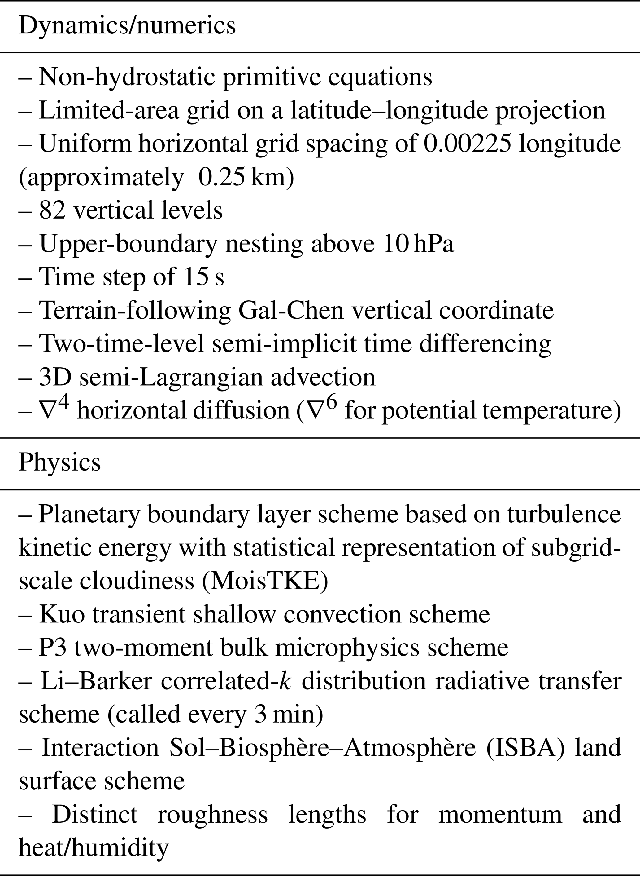
The model used in this study is the Global Environmental Multiscale (GEM) model (Côté et al., 1998; Girard et al., 2014). The GEM model is used for operational numerical weather prediction (NWP) by Environment and Climate Change Canada (ECCC) as well as research at ECCC and Canadian universities. The dynamical core of GEM is formulated based on the non-hydrostatic fully compressible primitive equations with a terrain-following hybrid vertical grid. As such, it can be run at cloud-resolving (sub-kilometre grid spacing) scales. It can be run on global or limited-area domains and is capable of one-way nesting. In this study, an idealized model configuration was used to simulate tropical deep convection, with a horizontal grid spacing of 250 m in a simulation domain of 160 km × 160 km, with 83 vertical levels over a tropical ocean surface. The horizontal grid spacing of 250 m is nearly at the cloud-resolving scale (Bryan et al., 2003; Lebo and Morrison, 2015). It is also close to the corresponding distances (110 to 180 m) of the 1 Hz in situ observational data from the aircraft which flew mostly at 110–120 m s⁻¹ (Convair 580) and 150–180 m s⁻¹ (Falcon 20). To resolve the vertical profiles near the tropical melting layer, vertical grid spacings of approximately 100 m were used between the altitudes of 4 and 7.5 km. The reader is referred to Table 1 for more details on the dynamics/numerics and physics configurations used in the model.

Table 1 Summary of the GEM model configurations' details. References to specific schemes are provided in Milbrandt et al. (2016).

The atmospheric initial conditions were horizontally homogeneous, based on an initial sounding taken from the operational global GEM analysis at 12:00 UTC on 15 May 2015 at 6.769^∘ N, 49.551^∘ W. The initial profile (Fig. 1) had 1697 J kg⁻¹ of convective available potential energy (CAPE). The GEM analysis also provided the initial sea surface temperature. The location and time were chosen based on the occurrence of an extensive mesoscale system that formed in this region and was observed (Fig. 2) during the HAIC-HIWC field campaign (Strapp et al., 2021).

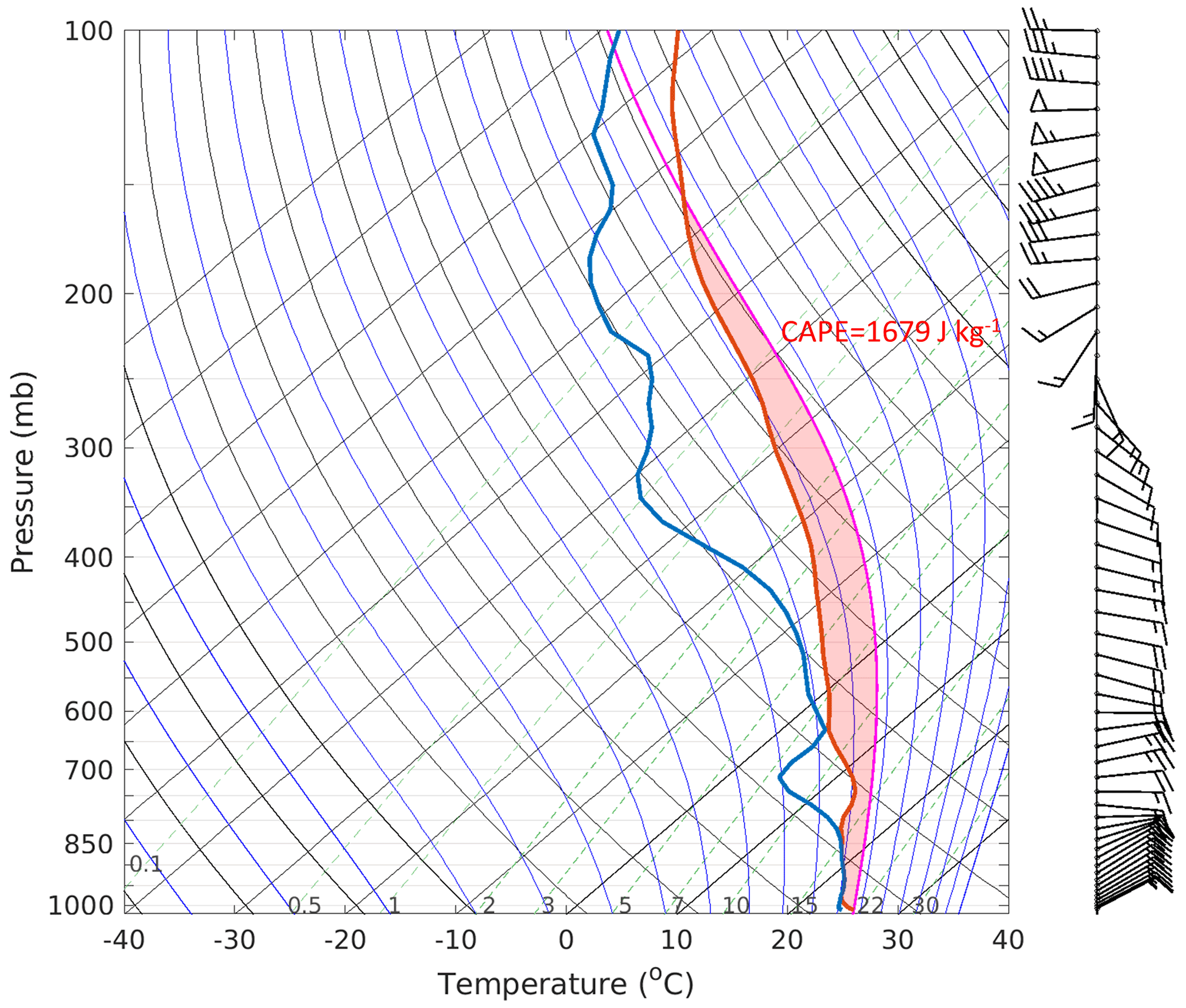
Figure 1 Initial atmospheric profiles for the idealized simulations. The blue line represents the dew point temperature, the red line represents the environment sounding (temperature), and the magenta line represents the parcel lapse rate.

To initiate the model storm, the updraft nudging method of Naylor and Gilmore (2012) was used to force convection during the first 15 min of the simulation. Three distinct updrafts were initialized 15 km apart from each other in the western part of the simulation domain. Each updraft was forced by perturbing the vertical air velocity (w_t) in a spheroid with a horizontal radius of 10 km and vertical radius of 1.5 km, centred at 1.5 km altitude, as shown in Eqs. (1) and (2).

$$\begin{array}{}\text{(1)}& {\displaystyle }{w}_{\mathrm{mag}}=\left\{\begin{array}{ll}{w}_{\max }{\cos }^{\mathrm{2}}\left(\frac{\mathit{\pi }}{\mathrm{2}}\mathit{\beta }\right)& \mathrm{if}\mathrm{0}\le \mathit{\beta }\le \mathrm{1},\\ \mathrm{0}& \mathrm{if}\mathit{\beta }>\mathrm{1}.\end{array}\right.\text{(2)}& {\displaystyle }{w}_t=w_{t-\mathrm{1}}+\mathrm{dts}\times \mathit{\alpha }\times \max (w_{\mathrm{mag}}-w_{t-\mathrm{1}},\mathrm{0}).\end{array}$$

Here, β is the distance from the centre of the spheroid normalized by its radius, α is an inverse nudging timescale (0.5 s⁻¹), dts is the model time step, and w_max is the maximum updraft speed (10 m s⁻¹) for nudging.

3.2 Cloud microphysics scheme

All cloud microphysical processes in the GEM simulations were represented by the P3 two-moment bulk microphysics scheme, where up to four (free) ice categories were used. For each ice category, there are four prognostic (i.e., advected) mixing ratio variables: the total ice mass, the rime mass, the bulk volume, and the total number. From the prognostic variable fields, various bulk physical properties can be computed. The size distribution of each category is represented by a complete gamma function. The liquid-phase component of P3 consists of two-moment categories for cloud droplets and rain. For details on the representation of each hydrometeor category and the parameterized microphysical processes, the reader is referred to Morrison and Milbrandt (2015); for details on the multi-category configuration, see Milbrandt and Morrison (2016).

It should be noted that there have been several further key developments to P3 since the first version of the multi-ice-category scheme, along with various minor modifications. Major developments include a triple-moment treatment of rain (Paukert et al., 2019), the introduction of a prognostic liquid fraction for wet ice (Cholette et al., 2019), and a triple-moment treatment of ice (Milbrandt et al., 2021). The version of P3 used in this study does not include these major modifications. The impacts of these components of P3 on SIP may be examined in future work. It is possible, for example, that triple-moment ice, which in principle results in a better representation of the PSD dispersion, may be important for some aspects of modelling SIP and its impacts. However, such work is outside of the scope of this study.

3.3 Parameterization of SIP

The following two SIP mechanisms were examined in this study. Other mechanisms will be considered in the future.

3.3.1 Rime splintering/Hallett–Mossop (HM)

The pristine version of P3 used in this study (i.e., prior to the SIP-related modifications examined here) includes a parameterization of the HM mechanism if two or more ice categories are used. The requirement for at least two categories is to prevent the dilution of ice particle properties when two populations of ice are forced to be represented by a single size distribution and set of physical properties (see Milbrandt and Morrison, 2016). The parameterized HM process produces a maximum of 350 ice crystals per milligram of collected liquid water, with crystal sizes of 10 µm, during riming of rain within a temperature range of −3 ^∘C > T > −8 ^∘C, with the peak value at −5 ^∘C and varying linearly to 0 ice crystals per milligram at the extreme temperature ranges. This ice multiplication parameterization has been used in several traditional (fixed-ice-category) microphysics schemes (e.g., Reisner et al., 1998). This is similar to the original HM parameterization in P3 as used in Milbrandt and Morrison (2016).

One modification to the HM parameterization in this study is to exclude the use of collected liquid water from the situation where raindrops (100 µm < D < 3500 µm) were collected/nucleated by small ice particles (D < 100 µm). From the point of view of the SIP mechanism, it is more appropriate to apply this part of collected liquid water to the FFD mechanism.

3.3.2 Fragmentation of freezing drops (FFD)

The parameterization of the FFD mechanism was implemented following Lawson et al. (2015):

$$\begin{array}{}\text{(3)}& N_f=\mathrm{2.5}\times {\mathrm{10}}^{-\mathrm{11}}{D}^{\mathrm{4}},\end{array}$$

where N_f is the average number of ice fragments per drop, and D is the drop diameter in micrometres. The parameterization of the FFD process was applied for raindrops (100 µm < D < 3500 µm) that were nucleated by ice particles (D < 100 µm). Following Keinert et al. (2020), the activity of the FFD process was limited to the temperature range of −25 ^∘C < T < −2 ^∘C. Within the temperature range, the current parameterization is not dependent on temperature. Further studies are being undertaken in order to explore the impacts of variation due to temperature.

3.3.3 Ice collection efficiency

Although not directly part of SIP, ice aggregation is another process that impacts N_i and may therefore be important in affecting high IWC. There are several different approaches to parameterize the ice collection efficiency, which is a key parameter in the aggregation parameterization (Hallgren and Hosler, 1960; Lin et al. 1983; Cotton et al., 1986; Ferrier et al., 1994, 1995; Milbrandt and Yau, 2005a, b; Seifert and Beheng, 2006). Khain and Pinsky (2018) showed that the collection efficiencies in these parameterizations vary by more than 2 orders of magnitude for any given temperature between −40 and 0 ^∘C. Sensitivity simulations conducted in the framework of this current study showed a high sensitivity of the modelled IWC and N_i to the collection efficiency of ice. The collection efficiency used in this study follows Cotton et al. (1986). Further discussion of the sensitivity of the modelling results to the ice aggregation parameterization is presented in Sect. 7.

4 Establishment of the control configuration

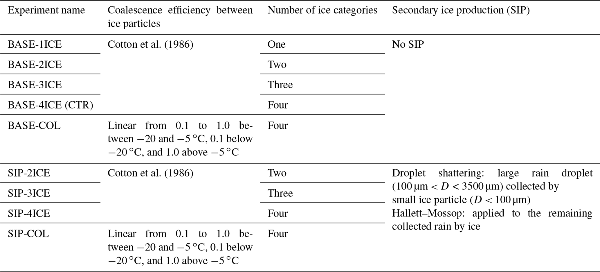
The number of ice categories used in the P3 scheme can impact the overall simulation results (Milbrandt and Morrison, 2016). SIP results in large quantities of small ice splinters, which can be co-located with pre-existing larger ice particles; thus, bimodal or multi-modal ice size distributions may occur. This cannot be represented with the single-ice-category configuration because P3 uses complete gamma size distributions for each hydrometeor category. Therefore, SIP – or any other ice initiation process – could result in the “dilution” of the bulk particle properties of existing ice where the microphysics scheme tries to represent two or more populations of ice particles within a single size distribution and with a single set of bulk physical properties (e.g., mean size). Thus, before examining the impacts of SIP in the simulation, a control configuration must be established based on the minimum number of ice categories needed to represent ice particle evolution in P3 with sufficient detail. This is determined by the number of categories beyond which adding more does not change the simulated average profiles for more than 15% of the fields of interest (e.g., IWC and N_i). To address this, a series of sensitivity tests was conducted (1) using the baseline version of P3 (with no SIP) and varying the number of ice categories from one to four and (2) using P3 with SIP included and varying the number of categories from two to four.

Table 2 summarizes the complete list of experiments conducted in this study. For the experiments starting with “BASE” (denoting the baseline P3 configuration), no SIP is activated. The experiments starting with “SIP” use the new parameterization for both the FFD and HM process. In the following analysis, we focus on the simulation results between 90 and 150 min, when the convective systems are more complex and more closely resemble the observed MCS.

Table 2 List of simulations.

As described in Sect. 3, three convective cells were initiated in the eastern part of the simulation domain. Figure 3 shows the upward longwave flux from the BASE-1ICE simulation at the top of the atmosphere (Fig. 3a, b, c, d) and the radar reflectivity of the vertical cross sections (Fig. 3e, f, g, h) indicated by black lines in Fig. 3a–d for simulation times of 30, 60, 120, and 180 min. The initial formation of the three convective updrafts can still be seen at 30 min (Fig. 3a). By 60 min, these updrafts started to merge, forming a larger system (Fig. 3b). This system then moved westward (towards the right of the domain) and developed into a sustained system (Fig. 3c). By 180 min, the convection began to weaken (Fig. 3d, h).

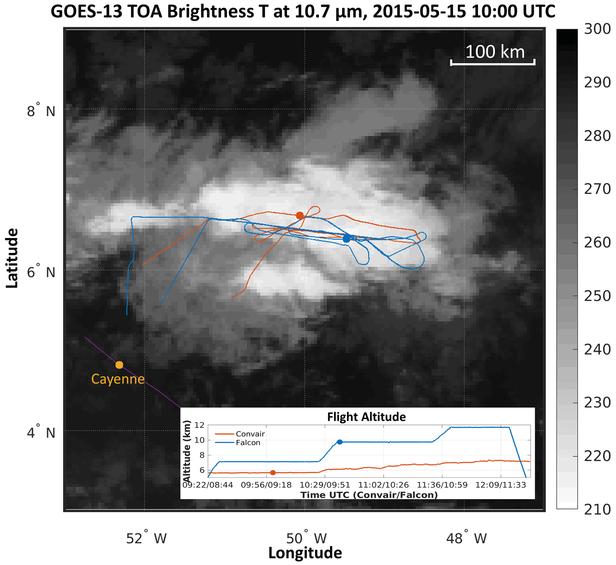
Figure 2 GOES-13 top-of-atmosphere (TOA) brightness temperature at 10.7 µm at 10:00 UTC on 15 May 2015 (Knapp et al., 2018). Blue lines denote the Falcon 20 flight track and altitudes; red lines denote the Convair 580 flight track and altitudes; red and blue dots indicate the locations and altitudes of the Convair 580 and Falcon 20 aircraft, respectively, at 10:00 UTC; and purple line represent the coastline.

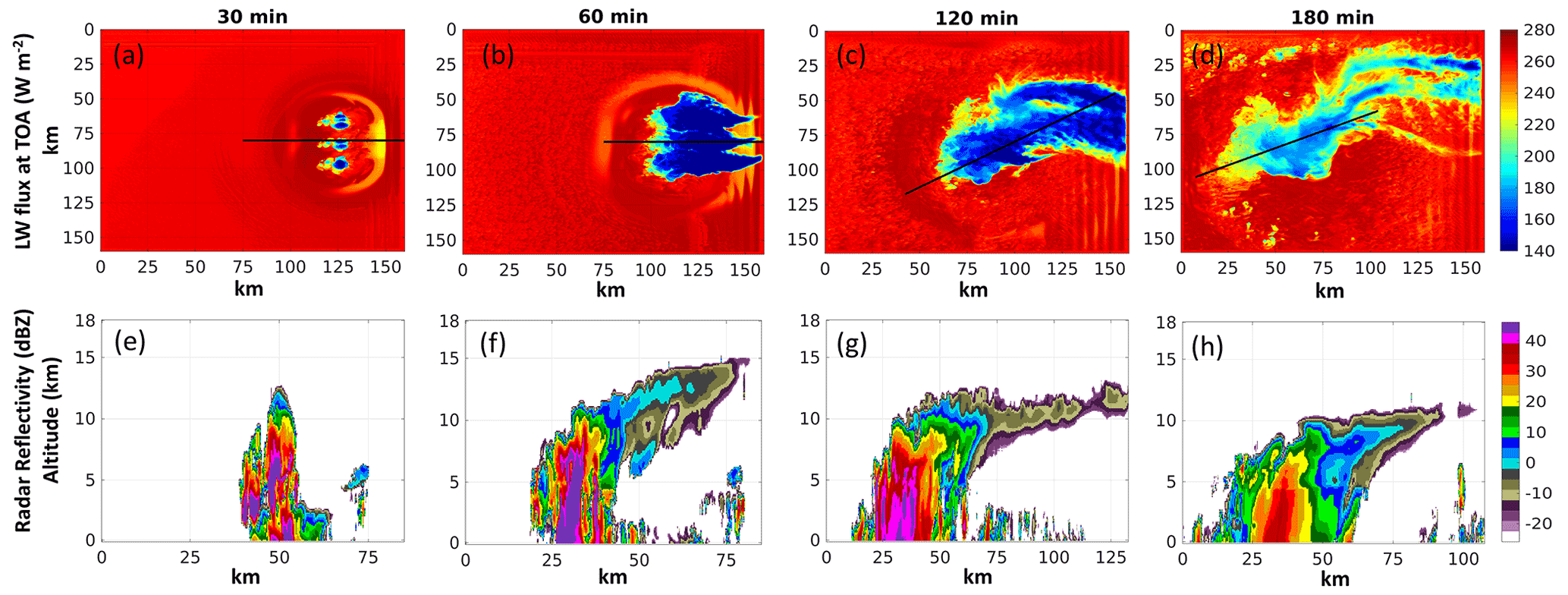
Figure 3 Simulation with a single ice category in the P3 bulk microphysics scheme for (a–d) upward longwave radiative flux at the top of atmosphere at four different times (30, 60, 120, and 180 min after the model initiation), and (e–h) the corresponding radar reflectivity of the cross section marked by the black line in panels (a)–(d).

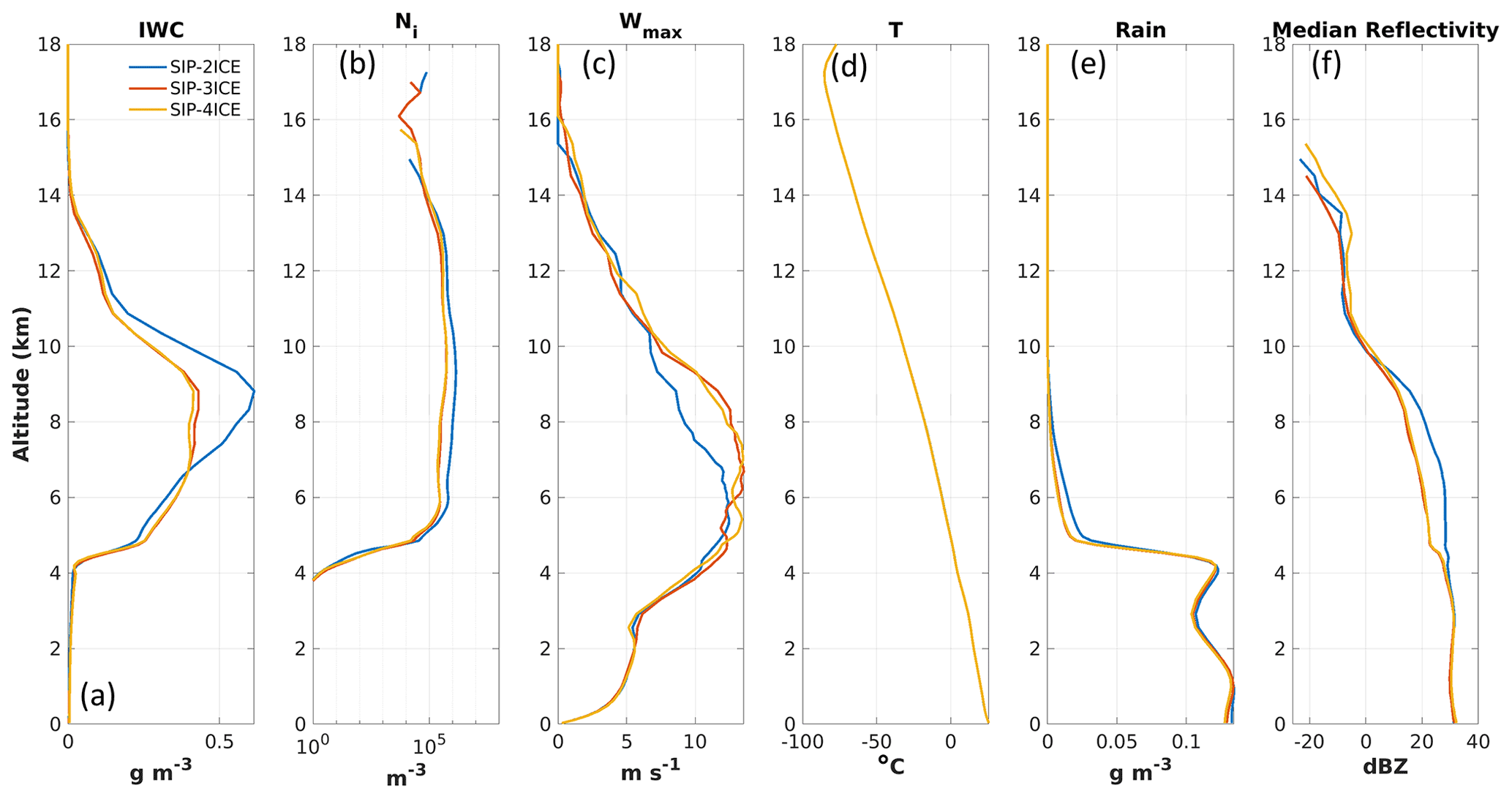
Figure 4 Profiles from the baseline simulations without SIP for (a) ice water content (IWC), (b) ice number concentration (N_i), (c) maximum vertical wind speed (W_max), (d) air temperature (T; the four simulations have only slightly different temperature that is not distinguishable in the figure), (e) rain water content (RWC), and (f) median radar reflectivity. The profiles are calculated based on data from 90 to 150 min of simulation. Panels (a) and (b) are horizontally averaged over regions with IWC > 0.001 g m⁻³, panel (c) is the horizontal maximum across the domain, panel (d) is a horizontal average over the whole domain, panel (e) is an average over the area with both ice water path and rain water path larger than 1 g m⁻², and panel (f) shows median values of reflectivity including points with either IWC or RWC larger than 0.01 g m⁻³ within the mask used for panel (e).

Figure 4 shows averaged profiles for the baseline simulations with different numbers of ice categories. The mean profiles of IWC (Fig. 4a) and N_i (Fig. 4b) consider all points with IWC larger than 0.001 g m⁻³. The maximum vertical wind speed (w_max; Fig. 4c) and average temperature profiles (Fig. 4d) apply to the entire model domain. The mean rainwater profiles are calculated based on data from the atmospheric columns in which both the ice water path and rain water path are larger than 1 g m⁻² (Fig. 4e). The radar reflectivity profiles (Fig. 4f) are the median values including points with either IWC or rain water content (RWC) larger than 0.01 g m⁻³ within the mask used for Fig. 4e.

For the altitude range between 5 and 12 km, adding one more ice category to the one-, two-, and three-category baseline simulations produces maximal changes of 12 %, 23 %, and 7 % for IWC, respectively (Fig. 4a). Similarly, maximal changes of 25 %, 31 %, and 14 % are found for N_i (Fig. 4b). The radar reflectivity (Fig. 4f) for the one-ice-category run (BASE-1ICE) is about 4 to 6 dBZ lower than the three- or four-category simulations in the same altitude range. This is likely caused by the fact that a single ice category is not sufficient to represent the coexistence of large and small ice particles and results in a reduction of the concentration of large ice particles, leading to lower radar reflectivity. With regard to the number of ice categories for SIP simulations, a similar conclusion to the baseline simulations was found. Adding one more ice category to two- and three-category SIP simulations produces maximal changes of 31 % and 9 % for IWC, respectively (Fig. 5a). For N_i, maximal respective changes of 70 % and 15 % are found (Fig. 5b). Therefore, at least three ice categories in P3 appear to be necessary and sufficient to examine the impacts of including SIP processes. Note that adding more ice categories for baseline and SIP simulations will not significantly change the morphology of the storm. It is of passing interest to note that the similarity of the three- and four-ice category results is consistent with the 1D kinematic simulations in Milbrandt and Morrison (2016). However, given that the use of more ice categories in P3 is generally preferable in principle (although there is added computational cost) and that four-ice-category simulations were already performed, BASE-4ICE is taken as the control run for the sensitivity studies to follow; this simulation is referred to as CTR. Correspondingly, we focus on the four-ice-category simulation including SIP (SIP-4ICE) for direct comparison to CTR.

Figure 5 Same as Fig. 4 but for the SIP simulation with two, three, and four ice categories.

5 Impacts of SIP on microphysical properties

5.1 Domain-averaged profiles

Figure 6 shows simulated average profiles for the four-ice-category simulation including SIP processes – SIP-4ICE (see Table 2) – as well as for CTR. As seen in Fig. 6a, the SIP-4ICE simulation has at least 100 % higher IWC compared with the control run above 6 km. SIP-4ICE has significantly higher N_i than CTR (Fig. 6b), with differences reaching 2–3 orders of magnitude near 6 km and about 1 order of magnitude above 11 km.

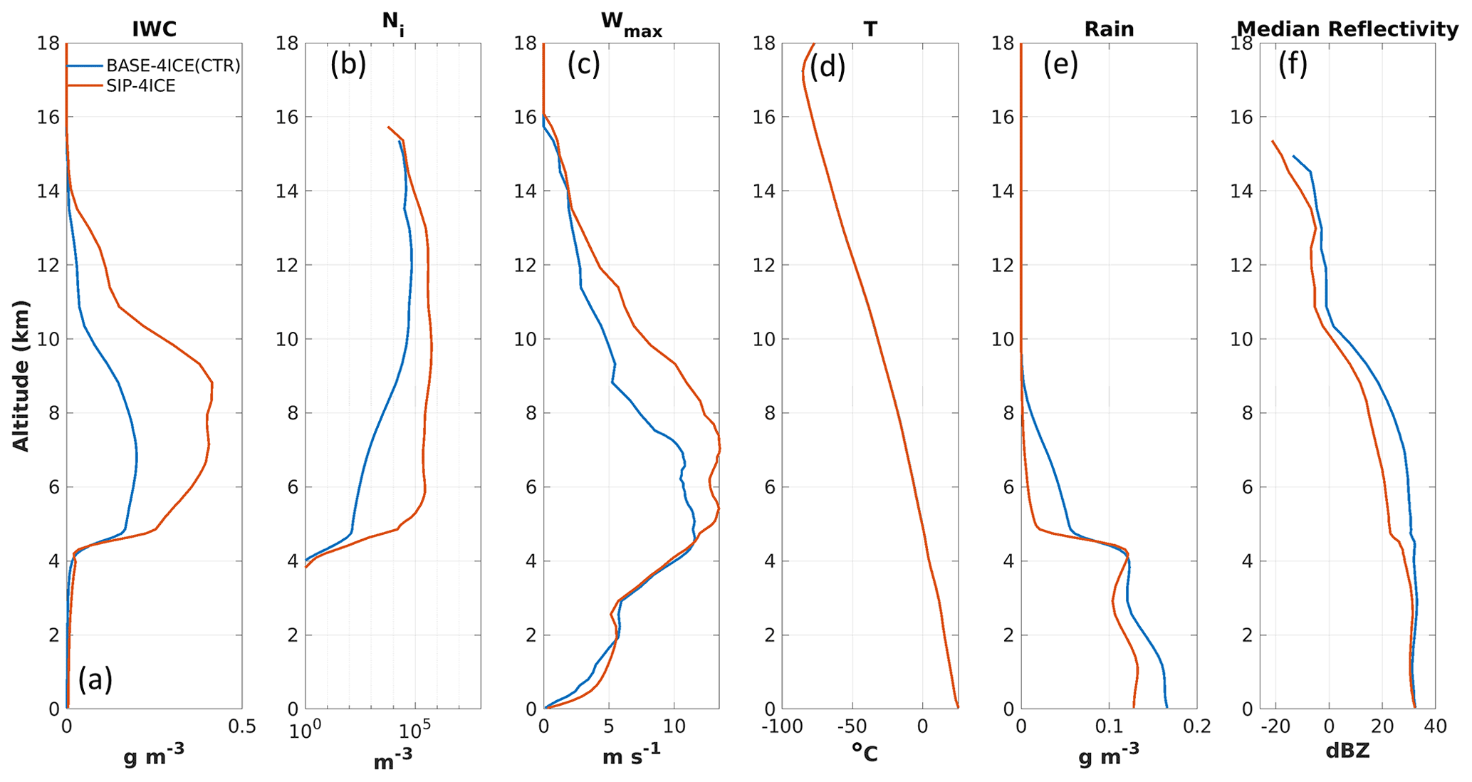
Figure 6 Same as Fig. 4 but for the baseline (CTR) simulation with four ice categories and the SIP simulation with four ice categories.

Figure 6c shows the maximum vertical air velocity in the domain. The simulations are very similar below the melting layer (∼4.5 km), but the w_max of SIP-4ICE is 2 to 5 m s⁻¹ higher above the melting layer. This suggests that SIP enhances convection due to the sudden production of a large number of small ice particles, resulting in the rapid freezing of rainwater and depletion of water vapour by diffusional growth. Both effects result in latent heating, which invigorates convection. This can be inferred from Fig. 6e, which shows that RWC in CTR is reduced from 0.12 g m⁻³ at 4.2 km to 0.05 g m⁻³ at 5 km, whereas RWC from SIP-4ICE is changed from 0.12 g m⁻³ at 4.2 km to 0.01 g m⁻³ at 5 km. Another potential mechanism of convection enhancement above the melting layer will be discussed in Sect. 6.

The medians of radar reflectivity of the SIP simulation is 5 to 10 dBZ lower compared with those of the CTR simulation between the altitudes of 5 and 12 km (Fig. 6f). This is because the SIP simulation has smaller ice particles, despite the higher IWC values, due to the higher N_i.

In order to confirm that the simulation differences illustrated in Fig. 6 are indeed the result of the inclusion of parameterized SIP processes, and not simply a chance set of changes that could result from perturbations in the model due to some minor code change, a set of 10 ensemble simulations were run for each configuration (CTR and SIP-4ICE) but with perturbed initial conditions. Figure 7 shows the ensemble results for the two configurations at 120 min. Each configuration includes 11 members (1 unperturbed and 10 perturbed members). The initial temperature profile is randomly perturbed with the maximum range of ±1 ^∘C at all model levels. The ensemble results show high consistency. The SIP simulation consistently produces much higher IWC and N_i. The vertical velocity w_max of an ensemble member is the single maximal value of a given model level. Therefore, the profiles of w_max can be noisy. The ensemble profiles of w_max for CTR and SIP-4ICE overlap, especially below the altitude of ∼6 km. However, the averaged maximal vertical velocity w_max (solid lines) diverges above the altitude of ∼6 km, which indicates that the SIP simulations generate stronger updrafts in general. The RWC and the radar reflectivity are both strongly reduced by 5 to 10 dBZ in the SIP simulations between 5 and 10 km. Similar remarks can be made for all other times between 90 and 150 min (not shown). The results summarized in Fig. 7 lend support to the idea that the differences between CTR and SIP-4ICE are indeed due to the effects of SIP on the microphysical and thermodynamic fields and are not merely another model realization of a chaotic weather system.

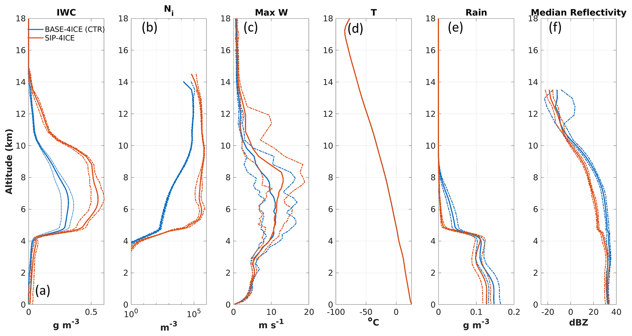
Figure 7 Same as Fig. 4 but showing the domain-averaged profiles for the CTR and SIP simulations with four ice categories, for 11 ensemble members each. The dot-dash lines show the minimum and maximum values among the ensemble members. The results are calculated based on data at 120 min after the model initiation.

5.2 Ice number concentration

Figure 8 shows comparisons of the probability density function of N_i, F(N_i), calculated from the simulations and measured during airborne in situ observations at two different altitude (H) ranges. The N_i measured in situ is calculated for the size range between 40 µm and 12.5 mm. The ice particles smaller than 40 µm are not counted due to large uncertainty of the instrument in that size range (Baumgardner et al., 2017). The F(N_i) values measured in situ were averaged over all HAIC-HIWC flights for the clouds with IWC > 0.01 g m⁻³. Figure 8a shows a comparison of F(N_i) at altitudes 6 < H < 7 km. The CTR simulation (blue line) shows a significant underestimation of N_i compared with the measured values (black line). The concentrations corresponding to the modal value of F(N_i) in CTR are nearly 2 orders of magnitude lower than those obtained from in situ observations. The SIP-4ICE simulation (red line) shows good agreement with the measured values.

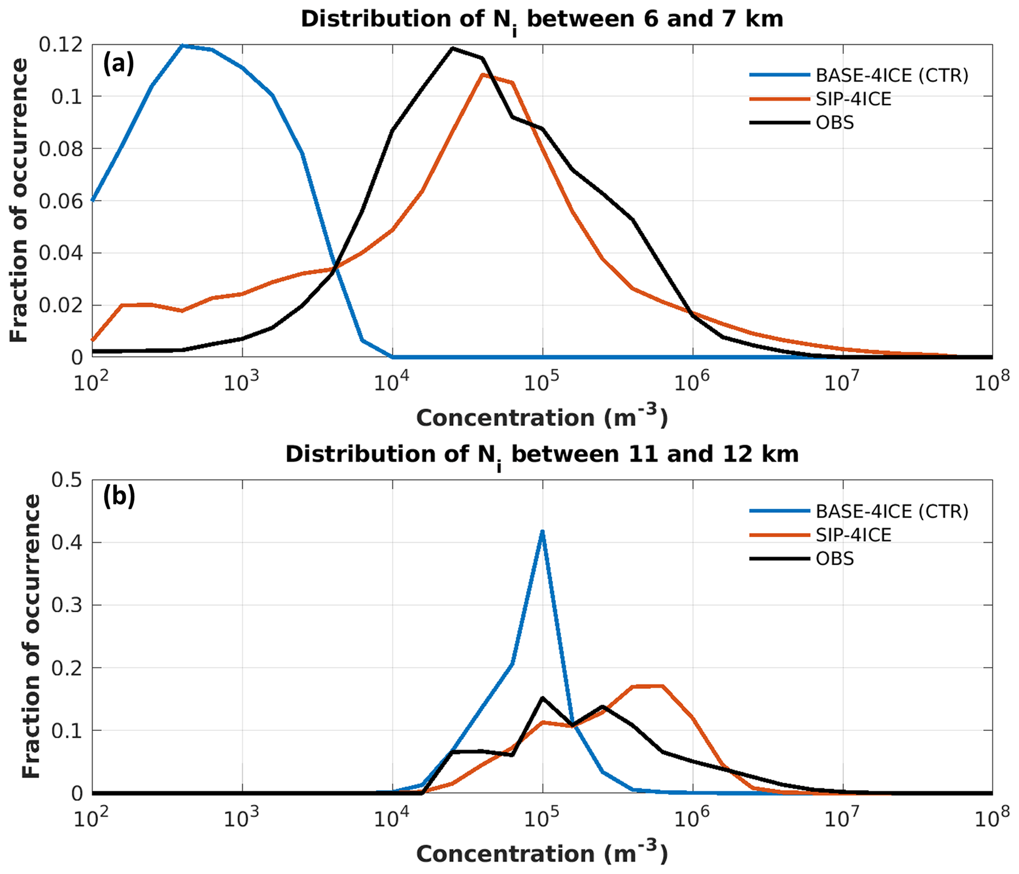
Figure 8 Distribution of N_i for model simulations and for the observational data from the HAIC-HIWC aircraft campaign near French Guiana in May 2015. A logarithmic bin width of $\mathrm{1}/\mathrm{5}$ of an order of magnitude is used. Panel (a) displays results from data between altitudes of 6 and 7 km and with an ice water content higher than 0.01 g m⁻³. Panel (b) is the same as panel (a) but for altitudes between 11 and 12 km.

The general behaviour of the functions F(N_i) for 11 < H < 12 km (Fig. 8b) is similar to that obtained for 6 < H < 7 km in Fig. 8a. The maxima of F(N_i) for CTR and observed values correspond to approximately the same ice concentrations of 10⁵ m⁻³. However, the maximum of F(N_i) in CTR is nearly triple that of the observed F(N_i) which was reasonably close to that of SIP-4ICE. The width of F(N_i) from SIP-4ICE agrees better with the observations than that from CTR. There are almost no grid points in CTR with a concentration above $\sim \mathrm{3}\times {\mathrm{10}}^{\mathrm{5}}$ m⁻³, whereas SIP-4ICE overestimated F(N_i) compared with the measured values. The overestimation of N_i of around 3×10⁵ m⁻³ is probably caused by uncertainty in the parameterizations of both the FFD process and the ice–ice collection efficiency. This warrant further studies on better quantifications of both processes.

5.3 Ice water content

Similar to the results discussed above, Figure 9 shows comparison of probability density functions of the IWC, F(IWC), obtained from model simulations and aircraft observations at altitudes 6 < H < 7 km (Fig. 9a) and 11 < H < 12 km (Fig. 9b). As seen in Fig. 9a, F(IWC) from SIP-4ICE is in good agreement with the observations for IWC values smaller than 3.25 g m⁻³. In contrast, the simulated frequency of encountering high IWC values in CTR is about $\mathrm{1}/\mathrm{2}$ to $\mathrm{1}/\mathrm{500}$ of the observed frequency between an IWC of 1 and 2 g m⁻³. There are no data with IWC values higher than 2.5 g m⁻³ in CTR.

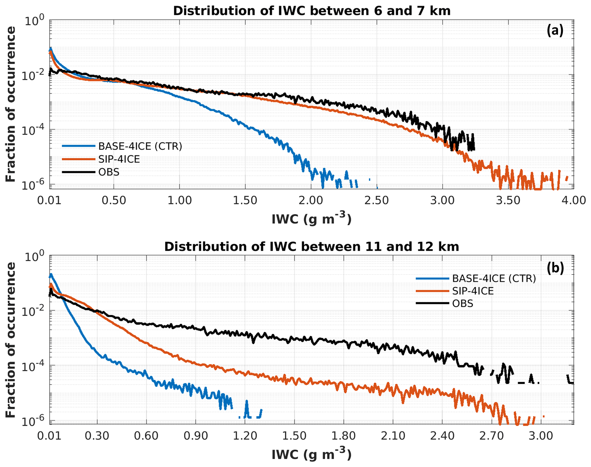
Figure 9 Distributions of ice water content (IWC) from the model simulations and observational data from the HAIC-HIWC aircraft campaign near French Guiana in May 2015. The bin width of 0.01 g m⁻³ is used. Panel (a) displays results from between altitudes of 6 and 7 km and with observational data from the NRC Convair 580 aircraft, and panel (b) presents results between altitudes of 11 and 12 km and with the observational data from the SAFIRE Falcon 20 aircraft.

SIP-4ICE produces some points with IWC > 3.25 g m⁻³, which were not observed by the instruments. The F(IWC) of these high IWC conditions from SIP-4ICE are below $\mathrm{1.7}\times {\mathrm{10}}^{-\mathrm{5}}$. For the Convair 580 aircraft, the number of observed 1 s average data points with IWC > 0.01 g m⁻³ is 59 893. This sets the limit of F(IWC) of the observational data at $\mathrm{1.7}\times {\mathrm{10}}^{-\mathrm{5}}$. If the campaign lasted much longer, it is conceivable that these high-IWC conditions might have eventually been observed.

Figure 9b shows similar results but for higher altitudes (between 11 and 12 km). The frequency of IWC values between 0.3 and 1.3 g m⁻³ in CTR is about 2–3 orders of magnitude lower than the observed frequency. There are no data with IWC values higher than 1.30 g m⁻³ from CTR. SIP-4ICE produces closer estimates compared to the observational data, as they both have IWC values up to ∼3 g m⁻³. Between 11 and 12 km, N_i of SIP-4ICE is considerably improved compared with CTR, as shown in Fig. 8b. However, the IWC of SIP-4ICE at these altitudes is still underestimated by 1–2 orders of magnitude beyond an IWC of 0.7 g m⁻³ compared with the observation. One possible reason for this underestimate is the differences in the sampling of data. At higher altitudes, between 11 and 12 km, there are often extensive areas with thin ice clouds near the convection. The data from SIP-4ICE used in the statistics include these areas if the IWC of the grid cell is larger than 0.01 g m⁻³. In contrast, the HAIC-HIWC campaign targeted conditions with a high IWC. The thinner ice clouds with IWC values between 0.01 and 0.3 g m⁻³ might not have been sufficiently sampled, as they are less relevant to the extreme conditions causing safety issues for aviation. This difference might partly explain the higher F(IWC) below 0.3 g m⁻³ and the lower F(IWC) above 0.3 g m⁻³ for SIP-4ICE compared with the observations. Another possible explanation of the underestimation is the uncertainty in the strength of simulated convections. In this study, the maximal updraft nudging speed w_max= 10 m s⁻¹ is used as the default value. Simulations with different w_max values are also tested. Using w_max= 15 m s⁻¹ in the SIP-4ICE simulation will produce a 63 % higher averaged IWC between 10 and 11 km than that produced by the default SIP-4ICE simulation with w_max= 10 m s⁻¹. For the SIP-4ICE simulation, the impact of w_max for lower altitudes between 6 and 7 km is negligible. The CTR simulation with w_max= 15 m s⁻¹ produces a higher IWC compared with the default CTR simulation with w_max= 10 m s⁻¹ (20 % and 50 % higher for altitudes range of 6–7 and 10–11 km, respectively). However, these values are still significantly smaller than those of the default SIP-4ICE simulation.

5.4 Longwave radiation and radar reflectivity

Figure 10 shows the upward longwave radiative flux at the top of atmosphere (TOA) for three different simulation times (90, 120, and 150 min) from CTR (Fig. 10a, b, c) and SIP-4ICE (Fig. 10d, e, f). The lowest TOA flux of SIP-4ICE is on average 11.4 ^∘C lower than that of CTR. The surface of area with TOA longwave flux lower than 170 W m² for SIP-4ICE is on average 2.7 times larger than that of CTR. This suggests that the cloud tops with SIP included are higher (Fig. 10d, e), and the anvil clouds are more extensive (Fig. 10e, f).

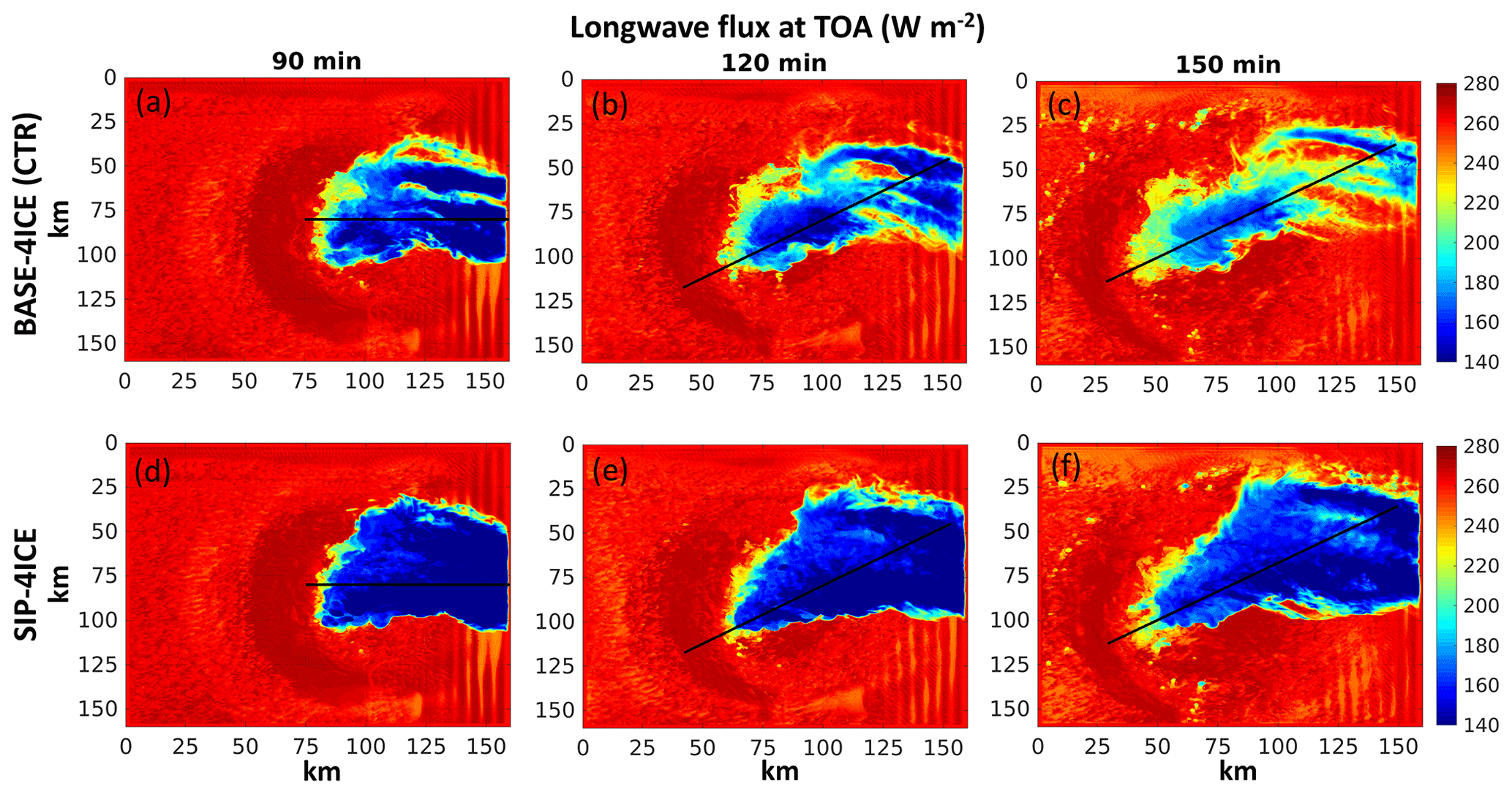
Figure 10 Longwave flux at the top of atmosphere for (a–c) the simulation with the baseline GEM set-up with four free categories of ice at 60, 120, and 180 min after the initiation. Panels (d)– (f) are the same as panels (a)– (c) but for the simulation with SIP implemented. Black lines indicate the location of the cross sections shown in later results.

Figure 11 Simulated radar reflectivity for the cross sections indicated by the black lines in Fig. 10.

The corresponding simulated radar reflectivity of the cross section indicated by the black lines in Fig. 10 is shown in Fig. 11. One significant difference between the CTR (Fig. 10a, b, c) and SIP-4ICE (Fig. 10d, e, f) simulations is that the reflectivity from the simulation with SIP is significantly lower than that of the control run between altitudes of approximately 5 and 10 km. This is due to the higher N_i values and, thus, smaller ice particle sizes in SIP-4ICE.

Figure 12 shows a comparison of the frequency distribution of radar reflectivity for CTR and SIP-4ICE (Fig. 12a, b) and for the NRC Convair 580 X-band radar (Fig. 12c). For the results of the two simulations, only the atmospheric columns with both ice water path and rain water path values larger than 1 g m⁻² are selected. The X-band radar data in Fig. 12c were averaged over all research flights during the HAIC-HIWC campaign. Figure 12d shows the simulated and observed median values of the reflectivity. At altitudes higher than 10.3 km, reflectivity in both the CTR and SIP-4ICE runs is lower than the measured reflectivity. However, between 5 and 10 km, SIP-4ICE has values closer to the observations, with a maximum overestimation of 4 dBZ at 5 km. CTR clearly overestimates the reflectivity by 5 to 15 dBZ between 5 and 10 km.

Figure 12 Radar reflectivity distribution frequency for (a) CTR with four ice categories between 60 and 180 min after model initiation. Panel (b) is the same as panel (a) but for the model with SIP included. Panel (c) is from all of the observational data from the NRC Convair 580 aircraft during the HAIC-HIWC campaign. Panel (d) is the median value for each altitude for the two model simulations and observations.

Figure 13 A 2D histogram of N_i and reflectivity (a, c, e) and of IWC and reflectivity (b, d, f). Panels (a) and (b) show BASE-4ICE (CTR), panels (c) and (d) show SIP-4ICE, and panels (e) and (f) show observations. The data between altitudes of 6 and 7 km are used. For the model simulation, the data between 90 and 150 min are used. The radar reflectivity data from the Convair 580 are the averaged values of the closest upward- and downward-pointing measurements.

For SIP-4ICE between 5 and 8 km, there is a large number of cases with reflectivity larger than 25 dBZ; this is not found in the observations. Figure 13 shows the comparison of N_i and IWC against reflectivity for CTR (Fig.13a, b), SIP-4ICE (Fig.13c, d), and the observations (Fig.13e, f). Although the distributions of N_i and IWC simulated using SIP-4ICE are closer to the observations than those of CTR, a significant number of cases (35.8 %) from SIP-4ICE still have reflectivity values larger than 25 dBZ, whereas only 0.4 % of the observations are above 25 dBZ.

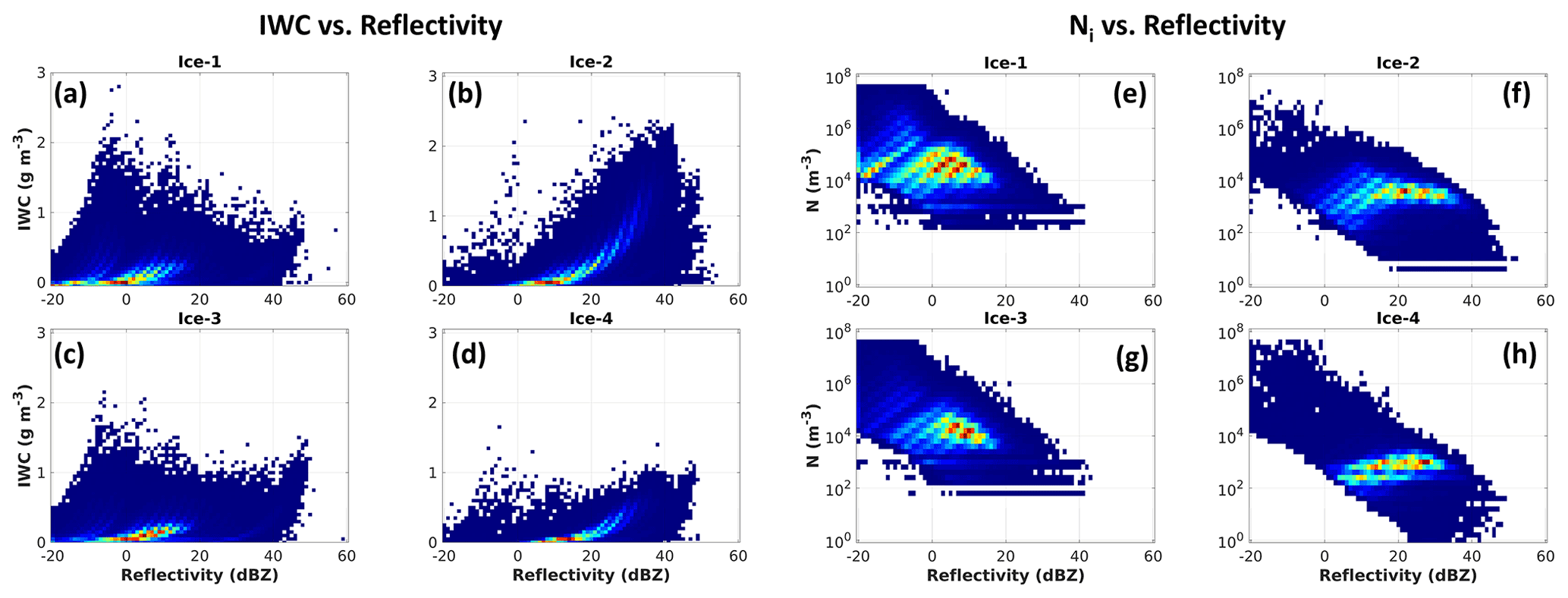
Figure 14 A 2D histogram of IWC and reflectivity (a–d) and of N_i and reflectivity (e–h) for each of the four ice categories. All results are for the SIP-4ICE simulation between 6 and 7 km and between 90 and 150 min.

Figure 14 shows the 2D histograms for the IWC and reflectivity (Fig. 14a, b, c, d) and for the N_i and reflectivity (Fig. 14e, f, g, h) for each of the four ice categories in SIP-4ICE. The ice categories 1 and 3 have generally lower reflectivity (1 % and 3 % higher than 25 dBZ, respectively) and higher N_i (peak value at 10^4.4 and 10⁴ m⁻³, respectively). By contrast, ice categories 2 and 4 have higher reflectivity (23 % and 24 % higher than 25 dBZ, respectively) and lower N_i (peak value at 10^3.4 and 10^2.8 m⁻³, respectively). This means that the ice particles in categories 2 and 4 have much larger mean sizes than those of categories 1 and 3. Most of the ice particles in categories 2 and 4 with reflectivity larger than 25 dBZ are lightly rimed aggregated ice with a rime fraction of ∼20 %. The mean-mass diameter of these ice particles could reach several millimetres. It is probable that the high reflectivity values (above 25 dBZ) are the result of these large ice sizes.

Several possible reasons could explain the high reflectivity in the model simulation. Firstly, the model might overproduced large ice particles due to an excessively large ice–ice collection efficiency (which is a highly uncertain parameter). Despite the important role of the ice–ice collection process in clouds, there is no consensus in the scientific literature on how to quantify it. A further discussion on the impact of the ice–ice collection efficiency on the simulation results is presented in the Sect. 7. Secondly, the current P3 version uses a diagnostic shape parameter for the gamma size distribution of ice. The shape parameter, which is a measure of the relative spectral dispersion, might give a wide distribution that implies too many large ice particles and, hence, higher reflectivity. Note that higher moments such as reflectivity are more sensitive to the tail of the size distribution. The triple-moment version of P3 (Milbrandt et al., 2021) uses a prognostic shape parameter that, in principle, should give better size distributions for those large ice particles. However, this comparison is beyond the scope of the current study, as the triple-moment version of P3 was not yet available when this current study began. Finally, the P3 scheme uses a Rayleigh scattering approach to calculate the radar reflectivity. It is not an advanced instrument simulator that can consider the attenuation, multiple and Mie scattering, etc. For the X-band radar on Convair 580, ice particles of several millimetres in size are in a transition region between Rayleigh and Mie scattering that is not symmetric but has a stronger forward-scattering lobe. Therefore, simulating the radar reflectivity with a Rayleigh scattering approach might overestimate the reflectivity for large ice particles. The radar reflectivity is a useful indicator to understand the model performance; however, considering that a rigorous instrument simulator is not used in this study, it is better to be cautious with regard to the comparison with the reflectivity.

Note that, at the altitude of the melting layer (∼ 4.5 km), none of the simulations reproduce the distinct bright band that is clearly apparent in the observational data. This is due to the fact that the version of P3 used in this study does not properly represent the transition state of melting ice with a wet surface and ice core (nor does P3 artificially boost the reflectivity contribution from ice during melting in order to mimic a bright-band effect). As mentioned in Sect. 3.3, a newer version of P3 includes a prognostic variable for the liquid mass content for each ice-phase category that allows for mixed-phase particles and a corresponding improvement in the calculation of reflectivity in the melting zone (which is to be shown in a forthcoming publication).

5.5 Vertical Doppler velocity

The Doppler velocity from the simulation is calculated using the mass-weighted fall speed of all hydrometeors subtracted from the vertical wind speed. Figure 15 shows the simulated Doppler velocity for CTR and SIP-4ICE for the vertical cross section shown in Fig. 11. The Doppler velocity below the melting layer is mostly negative due to the high fall speed of the rain. Above the melting layer, the average Doppler velocity gradually increases from −2 to 0 m s⁻¹ with altitude between 5 and 14 km. The gradual increase in the Doppler velocity is primarily linked to the size of ice particles. Positive values of the Doppler velocity are associated with convective cloud regions where the updraft velocity exceeds the falls speed of the ice particles. One difference between the control and SIP simulations is that the SIP-4ICE simulation has a higher Doppler velocity between 5 and 8 km for all three times analyzed.

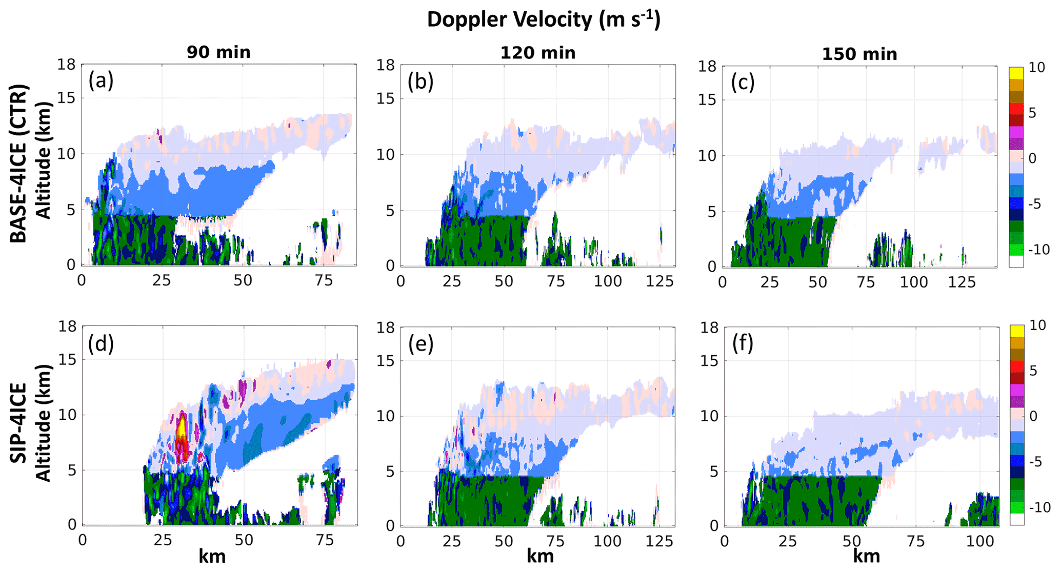
Figure 15 Simulated Doppler speed for the cross sections indicated by the black lines in Fig. 10.

Figure 16 Same for Fig. 12 but for the Doppler velocity.

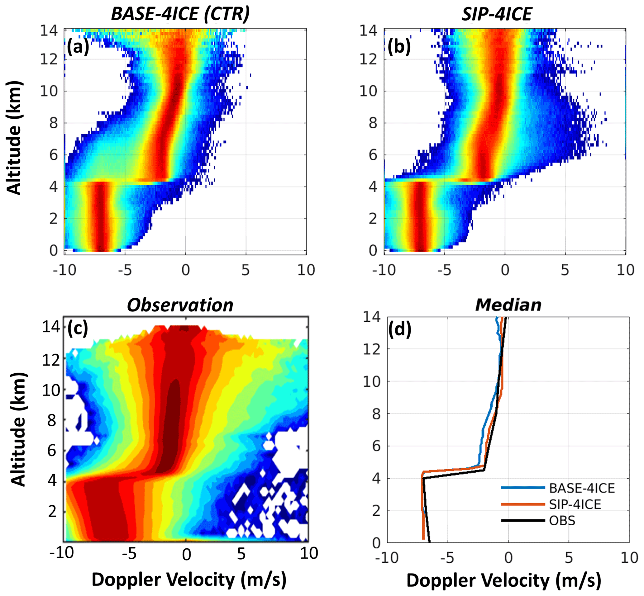
Figure 16 shows similar results to Fig. 12 but for the Doppler velocity. To mitigate the effect of anvils, the diagrams in Fig. 16a and b used the same mask as that for radar reflectivity in Fig. 12a and b. Both CTR (Fig. 16a) and SIP-4ICE (Fig. 16b) show distribution patterns very similar to those obtained from the observations (Fig. 16c). Figure 16d shows comparisons of the simulated and observed median values of the Doppler velocity vs. altitude. The SIP-4ICE simulation produces very close results to the measurements between the altitude of 5 and 9 km with maximum difference of ±0.3 m s⁻¹. The CTR simulation overestimates the negative Doppler velocity by approximately 0.9 m s⁻¹ compared with the measured values over the same range of altitudes. This result is consistent with the systematic underestimation of N_i in CTR and, therefore, overestimation of the mean particle sizes and fall speeds.

6 The role of SIP in tropical convection

In the previous section, it was shown that w_max is higher in the SIP-4ICE simulation than in the control simulation above the melting layer (Fig. 6c) and that the inclusion of SIP results in the enhanced formation of high-IWC regions above the melting layer. Altogether these results suggest that SIP plays an important role in the microphysics and thermodynamics of tropical convection, at least for the MCS examined. In order to explore SIP impacts in more detail, the rates and locations of SIP within the model storm and initiation of secondary convection are analyzed in this section.

6.1 SIP production at different altitudes

Figure 17 shows the active SIP areas and rates at different altitudes for the simulated MCS. Similar to Hu et al. (2021), the values of w are used to distinguish three different situations: (1) SIP within updrafts (marked by red lines, w > 3 m s⁻¹), (2) SIP within downdrafts (marked by yellow lines, w < 3 m s⁻¹), and (3) SIP with moderate vertical wind velocities (marked by blue lines, −3 m s⁻¹ $\le w\le$ 3 m s⁻¹).

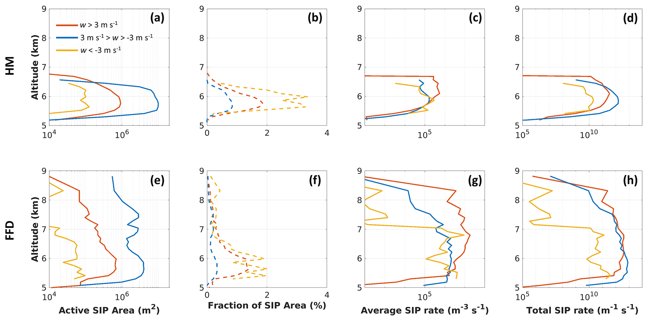
Figure 17 Panel (a) presents the area (in m²) with an active HM process; panel (b) presents the fraction of area with an active HM process; panel (c) displays the average rate of SIP by the HM process within the active area shown in panel (a); and panel (d) shows the total SIP rate, which is the product of panels (a) and (c). Panels (e)–(h) are the same as panels (a)–(d) but for the FFD process. Red lines (updrafts) denote SIP with w > 3 m s⁻¹, blue lines (outside of updrafts/downdrafts) denote SIP with w between −3 and 3 m s⁻¹, and yellow lines (downdrafts) denote SIP with w < −3 m s⁻¹. All results are temporal averages between 90 and 120 min.

For the employed SIP parameterizations, FFD is active in the range of altitudes 5 < H < 8.8 km (Fig. 17e), whereas HM occurs in a narrower range of 5.2 < H < 6.8 km (Fig. 17a). The range of the SIP activation altitudes is primarily determined by the temperature ranges of the FFD and HM processes (Sect. 2) as well as the temperature of the cloud base. The vertical velocity has a lesser effect on the SIP activation altitudes, and it may displace the upper and lower boundaries of the SIP regions within approximately ±200 m. Within these altitude ranges, SIP is mostly found in the area with moderate vertical wind velocities, followed by the area within updrafts, and occurs less in downdrafts for both the HM and FFD processes (Fig. 17a, e). The active SIP areas of FFD are usually smaller than those of the HM process in the range of altitudes 5.5 < H < 6.2 km for all three situations. To activate the FFD process, the employed parameterization requires the presence of large raindrops (100 µm < D < 3500 µm) as well as the presence of small ice particles (D < 100 µm). This condition likely restricts the FFD process to a smaller area than that of the HM process.

The vertical wind speed has a significant impact on the rate of SIP. Figure 17g shows the average SIP rates (m⁻³ s⁻¹) within the active FFD areas shown in Fig. 17e. For most altitudes, the rate of FFD increases with an increase in w, and it is at least 1 order of magnitude higher in updrafts than in downdrafts. This is related to the lower number of precipitation-sized drops in downdrafts compared with updrafts.

Another factor is related to the effect of w on the residence time of drops within the range of the SIP activation altitude ΔH. For a drop with a terminal fall velocity V_fall(D), the residence time can be assessed as follows: $\mathit{\tau }=\mathrm{abs}\left(\mathrm{\Delta }H/\left(V_{\mathrm{fall}}\right(D)-w)\right)$. Depending on the sign of (V_fall(D)w), the drop will be moved upward through ΔH or downward. For the extreme situation when V_fall(D)= w, the drop is suspended in an updraft indefinitely, and it can freeze and generate secondary ice or mechanically interact with other cloud particles, thereby changing its fall velocity.

The rate of the HM process (Fig. 17c) is higher in updrafts above 6.0 km where the riming process is active. At altitudes below 6.0 km, the rates are similar in updrafts, downdrafts, and areas with moderate vertical velocities (−3 m s${}^{-\mathrm{1}}\le w\le$ 3 m s⁻¹). Figure 17d shows the total SIP rate (m⁻¹ s⁻¹) from the HM process; this is the product of the surface of the area with an active HM process and the mean SIP rate from the HM process, as shown in Fig. 17a and c. The total SIP rate shows how many ice particles are produced by SIP horizontally across the domain per 1 m of vertical layer per second. The total SIP rate from the FFD process is shown in Fig. 17h. Below an altitude of 6.3 km, both the HM and FFD processes in the areas with moderate vertical wind velocities show the highest total SIP rate, followed by the area within updrafts. The lowest total rates are found in downdrafts. The larger active SIP areas associated with moderate vertical wind velocities (Fig. 17a, e) contribute significantly to the high total SIP rates across the domain. At altitudes above 6.3 km, updraft regions contribute more to the total SIP rates. This is due to the high average rates in updrafts (Fig. 17c, g), as the corresponding SIP areas are smaller than those with moderate vertical velocities.

The results obtained show that the vertical extent ΔH of FFD is deeper and its rate is higher than those of HM. This finding leads to the conclusion that the overall contribution of FFD to the production of the secondary ice in tropical MCSs is significantly higher than that of HM in the simulations in this study.

6.2 The role of SIP in initiating of secondary convection

The freezing of rain into ice and the vapour growth of ice splinters generate latent heating which should enhance the existing convection. This may explain the increase in w_max above 6 km in Figs. 6c and 7c in SIP-4ICE compared with CTR. As explained in the previous subsection, below 6.3 km altitude, both FFD and HM are more active outside of the major updrafts originating below the melting layer. High activity of the FFD and HM processes might eventually initiate new updrafts in stratiform regions inside MCSs above the melting areas.

A Lagrangian trajectory analysis was used to trace the cloud parcels affected by SIP. For this analysis, 1152 air parcels were selected with active SIP at an altitude of 5.6 km from the SIP-4ICE simulation between 90 and 150 min. Each selected parcel was traced backward (t < 0 min) and forward (t > 0 min) for 15 min (Δt= 30 min). These parcels were then classified into two different groups. The first group included the parcels that had altitudes within 5 < H < 6 km at t= −15 min and ended their trajectories at H > 6.5 km at t= 15 min. The second group included parcels with the same initial altitudes as the first group at t= 0 min; however, the altitude of their trajectories remained at H < 6 km at the end of forward tracing (t= 15 min). The total number of parcels of the first category was 47 and that of the second category was 1105.

Figure 18 shows the time history of mean values of environmental and microphysical parameters of the parcels for the two categories. Most parcels that underwent SIP processes between −5 and 5 min were located at the same altitude of 5.6 km at t= 0 min. These parcels started to rise from t= −3 min, and they eventually reached 7.5 km at t= 15 min (Fig. 18c). On the other hand, the other group of parcels did not rise throughout the 30 min analysis period (hereafter named “non-rising parcels”). The mean altitude of these parcels decreased by about 700 m (Fig. 18c).

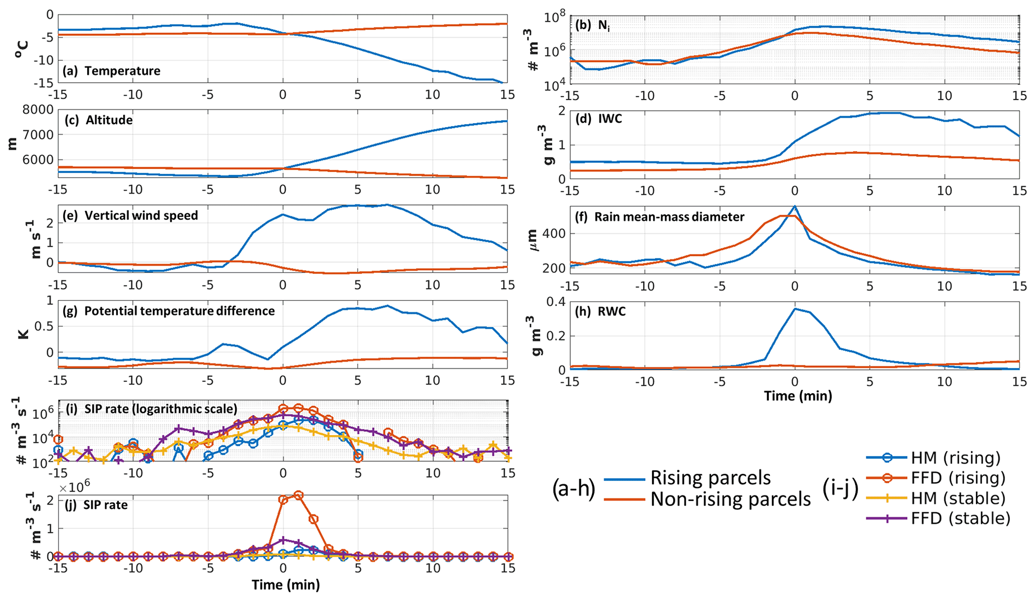
Figure 18 Trajectory tracing of different variables for the rising parcels (blue lines in a–h) and the non-rising parcels (red lines in a–h) for (a) temperature, (b) N_i, (c) altitude, (d) IWC, (e) vertical wind speed, (f) rain mean-mass diameter, (g) Δθ, (h) RWC, (i) SIP tendency in logarithmic scale, and (j) SIP tendency in regular scale.

Figure 18e shows that the rising parcels had an initial positive vertical speed from t= −3 to −1 min. However, their potential temperature differences with respect to the environmental values at the same altitudes (Δθ) were generally negative for t < −1 min and decreased slightly from t= −3 to −1 min (Fig. 18g). Thus, these parcels were not gaining positive buoyancy at this stage. However, the Δθ of the rising parcels started to increase quickly between t= 0 min and 2 min, becoming positive and reaching a difference of nearly +1 K between t= 3 and 8 min (Fig. 18g). Figure 18i and j also show very high SIP rates for the rising parcels from the FFD process during this time period. For the non-rising parcels, there was an increase in Δθ during the same period but at a much slower rate due to a smaller SIP tendency (Fig. 18i, j). The Δθ remained negative during the whole analysis period; therefore, these parcels were convectively stable.

The main reason for the high SIP rate between t= 0 and 2 min for the rising parcels is that there was a substantial amount of large rain drops available for activating the FFD process (Fig. 18f, h). The rain mean-mass diameter at t= 0 min was large (560 µm). The RWC was also large (0.36 g m⁻³). The rain mean-mass diameter for the non-rising parcels (502 µm) was slightly smaller than that of rising parcels at t= 0 min. However, the corresponding RWC was quite low (0.02 g m⁻³). With a large RWC and rain mean-mass diameter, the rising parcels had a high SIP potential, which eventually led to greater N_i, vapour growth, and increased latent heating and buoyancy, thereby enhancing secondary convection.

As mentioned in Sect. 6.1, the FFD process plays a dominant role in SIP compared with the HM process in the simulations of this study. This agrees with what we found in Fig. 18i and j. The sudden increase in the Δθ with respect to the environment is more likely linked to the high SIP rate from FFD. Therefore, SIP, in particular FFD, may play a role in the initiation of new updrafts above the melting layer.

Figure 19 shows an example of a rising air parcel. The black line represents the parcel trajectory from t= −15 to 15 min. From t= −15 to 0 min, the air parcel had no significant change in altitude. Near t= 0 min, the air parcel was close to an existing updraft (Fig. 19a, red surface) and was in an area where there was rainwater (Fig. 19b, red surface). Shortly after t= 0 min, the air parcel started to rise. The supply of rainwater resulted in an enhanced SIP and led to a higher rate of latent heating and rapid increase in buoyancy.

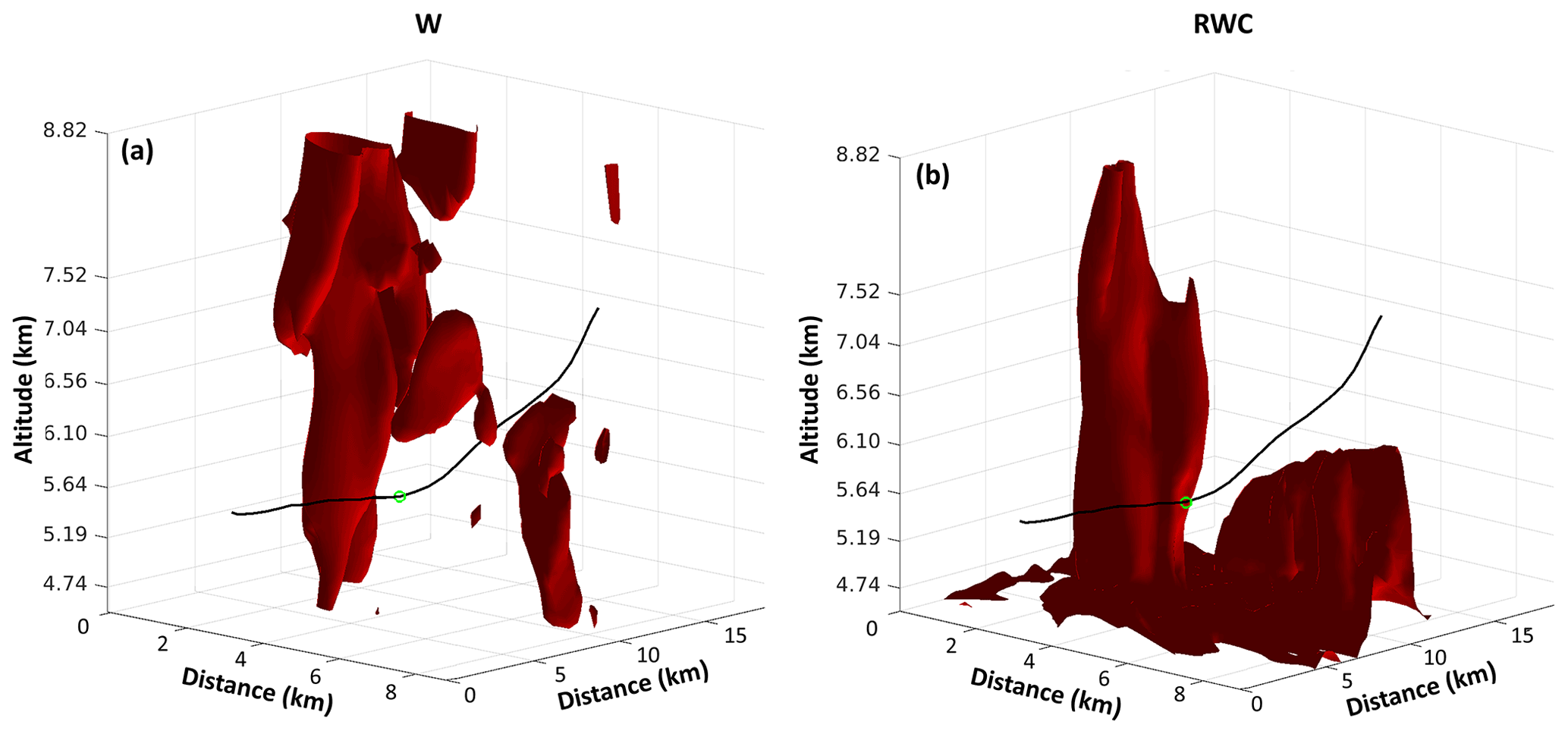
Figure 19 The trajectory of a specific air parcel (black line), and the location of the parcel at t = 0 min (green circle). The red surfaces in panel (a) show the area with w larger than 3 m s⁻¹ at the moment of t = 0 min, and red surfaces in panel (b) show the area with RWC larger than 0.05 g m⁻³ at the moment of t = 0 min.

7 Impact of ice aggregation

In addition to SIP, which clearly has significant effects on N_i, the formation of high IWC, radar reflectivity, and vertical wind velocity, the aggregation of ice particles also plays an important role in determining the microstructure. Aggregation results in a decrease in N_i and an increase in radar reflectivity and particle fall velocity. The rate of aggregation is characterized by the ice–ice collection efficiency (e_ii). In the framework of this study, the following parameterization of the ice–ice collection efficiency has been employed (Cotton et al., 1986):

$$\begin{array}{}\text{(4)}& e_{\mathrm{ii}}=\min ({\mathrm{10}}^{\mathrm{0.035}\left(T-\mathrm{237.16}\right)-\mathrm{0.7}},\mathrm{0.2}),\end{array}$$

where T is the temperature in kelvin.

There is a diversity of parameterizations of e_ii employed in models (Khain and Pinsky, 2018), which may vary by up to 3 orders of magnitude. In this study, the mid-range e_ii in Eq. (4) is used as the default parameterization. However, the uncertainty in e_ii raises a question about the impact of the ice aggregation parameterization on the N_i and high IWC formation.

To explore the effect of the ice aggregation rate on the high IWC formation, a sensitivity test (SIP-COL) was performed with another e_ii parameterization, i.e.,

$$\begin{array}{}\text{(5)}& e_{\mathrm{ii}}=\left\{\begin{array}{ll}\mathrm{0.1}& \mathrm{for}T<-\mathrm{20}{}^{\circ }\mathrm{C};\\ \mathrm{0.06}T+\mathrm{1.3}& \mathrm{for}-\mathrm{20}<T<-\mathrm{5}{}^{\circ }\mathrm{C};\\ \mathrm{1}& \mathrm{for}-\mathrm{5}<T<\mathrm{0}{}^{\circ }\mathrm{C}.\end{array}\right.\end{array}$$

As seen from Eq. (5), the new e_ii varied linearly from 0.1 to 1.0 within the −20^∘ < T < −5 ^∘C temperature range: for T < −20 ^∘C, e_ii= 0.1; for −5 ^∘C, <T < 0 ^∘C e_ii= 1.0. For all temperatures, e_ii in Eq. (5) is much higher than that in Eq. (4). We want to use this high e_ii parameterization to show the significant impact of e_ii on the simulation results.

Comparisons of the distributions of N_i for two SIP simulations with varying e_ii and the observations are shown in Fig. 20. For the altitudes between 6 and 7 km, using the new parameterization of aggregation (given by Eq. 5) (SIP-COL) results in a decrease in the modal value of F(N_i) by 2 orders of magnitude compared with using that described by Eq. (4) (SIP-4ICE). At higher altitudes between 10 and 11 km, the SIP-COL run produces ∼ 5 times higher F(N_i) at N_i values of 10⁵ m⁻³ and lower F(N_i) by 1–2 orders of magnitude for N_i > 4 × 10⁵ m⁻³ compared with those of SIP-4ICE.

Figure 20 Similar to Fig. 8 but for SIP-4ICE and SIP-COL.

Figure 21 Similar to Fig. 9 but for SIP-4ICE and SIP-COL.

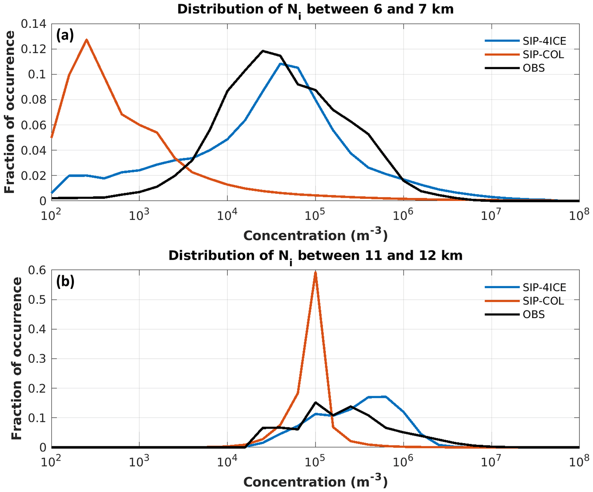
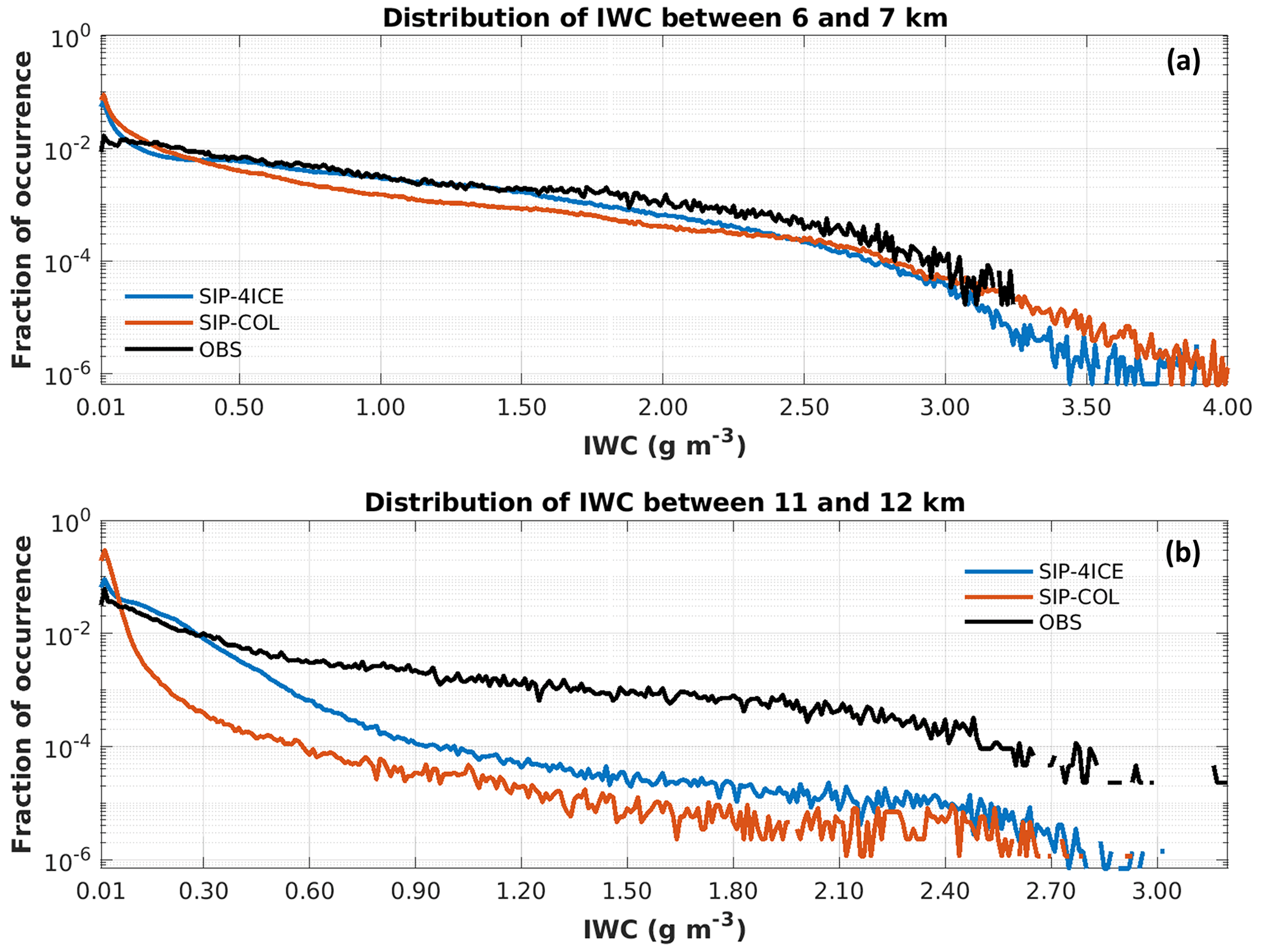
Figure 21 shows similar results to Fig. 20 but for the distribution of ice mass. Between 6 and 7 km, applying the linear approach for e_ii from Eq. (5) to the SIP-4ICE simulation (SIP-COL), the F(IWC) between 0.4 and 2.4 g m⁻³ is slightly reduced by up to 50 %. However, the F(IWC) for an extreme situation with an IWC value larger than 2.5 g m⁻³ is somehow slightly enhanced.

For altitudes between 11 and 12 km, the SIP-COL experiment produces a lower F(IWC), by up to ∼ 1 order of magnitude for most IWC values (> 0.16 g m⁻³), than the SIP-4ICE simulation. Although the estimation of F(IWC) by SIP-COL between 6 and 7 km is relatively close to that of SIP-4ICE, SIP-COL produces much lower F(IWC) at higher altitudes, between 10 and 11 km, than the SIP-4ICE simulation. This indicates that the N_i values at lower altitudes play an important role in determining the IWC at upper altitudes.

Figure 22 Similar to Fig. 6 but for simulation at a 1 km horizontal grid spacing.

8 Conclusion

The impacts of SIP on the microphysics and dynamics of deep convection have been examined using quasi-idealized near-cloud-resolving simulations of a tropical MCS based on storm observations during the HAIC-HIWC field campaign. GEM model simulations using the P3 microphysics scheme were conducted using a 250 m horizontal grid spacing and horizontally homogeneous atmospheric initial conditions, with updraft nudging to initiate convection. It was established through sensitivity tests that a minimum of three ice categories in P3 are necessary to examine SIP in detail; four categories were used for most of the simulations. P3 was modified to include rime splintering (HM) and fragmentation of freezing drops (FFD), which have been the most closely examined SIP mechanisms in laboratory studies. The parameterizations of the HM and FFD processes used were based on the information available from previously published results.

In the control configuration with no SIP processes at altitudes of 6 to 7 km, the simulated ice number concentrations were about 2 orders of magnitude lower than the values obtained from in situ measurements. The simulated frequency of encountering high-IWC conditions is about $\mathrm{1}/\mathrm{2}$ to $\mathrm{1}/\mathrm{500}$ of the observed frequency between IWC values of 1 and 2 g m⁻³. With the SIP mechanisms activated, the model results for these fields were dramatically improved compared with the observations. The Doppler velocities above the melting layer were also notably closer to the measured values, indicating improved ice fall speeds in the simulations with SIP active. SIP was responsible for an increase in the ice concentrations of up to 3 orders of magnitude at altitudes of 6 to 7 km. As a result, the total ice mass was distributed over a much larger number of particles; thus, the mean particle size was smaller with a lower fall speed. Consequently, ice was more easily transported to higher altitudes, ultimately resulting in sustained cloud regions with high IWC.

Analysis conducted in this study led to the following general conclusions for the high-resolution NWP simulations:

1. SIP processes play a critical role in the formation and maintenance of high IWC with low reflectivity at upper levels in MCSs.

2. SIP enhances secondary convection above the melting layer due to an increase in buoyancy caused by greater latent heat release during vapour deposition on numerous secondary ice particles. Enhanced secondary convection may, in turn, extend the longevity of MCSs and regions with high IWC.

3. Aggregation of ice particles results in a decrease in the ice number concentration and IWC at upper levels but is very sensitive to details of the parameterization of this process, in particular the collection efficiency, which remains uncertain.

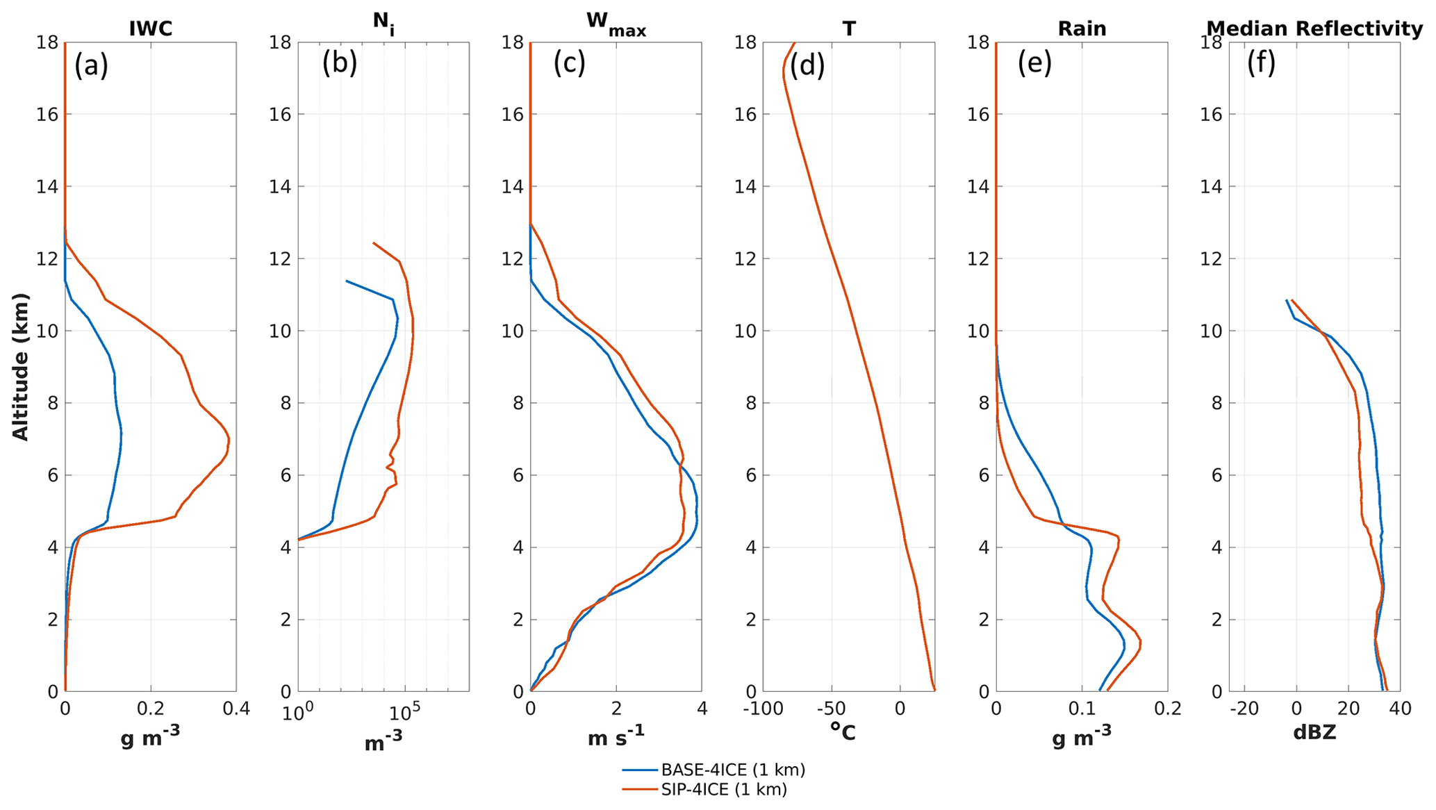
In order to minimize errors in the interpretation of the results due to unresolved convective updrafts, the simulations conducted in this study were all done with a horizontal grid spacing of 250 m. This is a much higher resolution than that of current operational NWP models; however, tests with a 1 km grid spacing (Fig. 22) indicated that the impacts of including SIP are very similar to those at a 250 m grid spacing, where 1 km is close to the grid spacing of several current operational and experimental NWP systems. Furthermore, the P3 microphysics scheme is already used operationally in the Canadian 2.5 km system (Milbrandt et al., 2015). Therefore, the conclusions regarding the importance of including SIP processes in models are not limited to numerical modelling in research mode but also have important implications for current and/or upcoming operational NWP, in particular for systems that provide numerical guidance for civil aviation operating at cruising altitudes between 10 and 14 km.

Finally, although the simulations conducted with the activated SIP process clearly resulted in improved results compared with the observations, this is not a basis for concluding that the HM and FFD parameterizations used are accurate representations of these physical processes. While the formulations were based on either laboratory experiments or combined modelling and in situ observational study, they are still largely ad hoc. This study further highlights the importance of these processes in deep convection and the need to include them in some fashion in numerical models. However, accurate parameterizations that capture the underlying physics of these mechanisms, not just their bulk effects, continue to be topics of research.