the Creative Commons Attribution 4.0 License.
the Creative Commons Attribution 4.0 License.
 | 19 Sep 2022
Modeling radiative and climatic effects of brown carbon aerosols with the ARPEGE-Climat global climate model
Thomas Drugé
Pierre Nabat
Marc Mallet
Martine Michou
Samuel Rémy
Oleg Dubovik
Organic aerosols are predominantly emitted from biomass burning and biofuel use. The fraction of these aerosols that strongly absorbs ultraviolet and short visible light is referred to as brown carbon (BrC). The life cycle and the optical properties of BrC are still highly uncertain, thus contributing to the uncertainty of the total aerosol radiative effect. This study presents the implementation of BrC aerosols in the Tropospheric Aerosols for ClimaTe In CNRM (TACTIC) aerosol scheme of the atmospheric component of the Centre National de Recherches Météorologiques (CNRM) climate model. This implementation has been achieved using a BrC parameterization based on the optical properties of Saleh et al. (2014). Several simulations have been carried out with the CNRM global climate model, over the period of 2000–2014, to analyze the BrC radiative and climatic effects. Model evaluation has been carried out by comparing numerical results of single-scattering albedo (SSA), aerosol optical depth (AOD), and absorption aerosol optical depth (AAOD) to data provided by Aerosol Robotic Network (AERONET) stations, at the local scale, and by different satellite products, at the global scale. The implementation of BrC and its bleaching parameterization has resulted in an improvement of the estimation of the total SSA and AAOD at 350 and 440 nm. This improvement is observed at both the local scale, for several locations of AERONET stations, and the regional scale, over regions of Africa (AFR) and South America (AME), where large quantities of biomass burning aerosols are emitted. The annual global BrC effective radiative forcing (all-sky conditions) has been calculated in terms of both aerosol–radiation interactions (ERFari, 0.029 ± 0.006 W m−2) and aerosol–cloud interactions (ERFaci, −0.024 ± 0.066 W m−2). This study shows, on an annual average, positive values of ERFari of 0.292 ± 0.034 and 0.085 ± 0.032 W m−2 over the AFR and AME regions, respectively, which is in accordance with the BrC radiative effect calculated in previous studies. This work also reveals that the inclusion of BrC in the TACTIC aerosol scheme causes a statistically significant low-level cloud fraction increase over the southeastern Atlantic Ocean during the burning season partially caused by a vertical velocity decrease at 700 hPa (semi-direct aerosol effect). Lastly, this study also highlights that the low-level cloud fraction changes, associated with more absorbing biomass burning aerosols, contribute to an increase in both solar heating rate and air temperature at 700 hPa over this region.
- Article
(45954 KB) - Full-text XML
- BibTeX
- EndNote


The representation of aerosols is still a fairly large source of uncertainty for climate models (Myhre et al., 2013; Szopa et al., 2021). In addition to affecting cloud properties and precipitation patterns (first and second indirect effects), some aerosols, such as black carbon (BC) particles, warm the atmosphere by directly absorbing solar radiation, while others, such as sea-salt or nitrate particles, tend to scatter it, which leads to cooling of the atmosphere (Haywood and Boucher, 2000; Bond et al., 2013; Zhang et al., 2020). In modeling studies, organic aerosols (OA, also referred as organic matter, OM), which include primary organic aerosols (POA) and secondary organic aerosols (SOA), are usually considered to be strongly scattering (Myhre et al., 2013). However, recent works have shown that a part of the OA, known as brown carbon (BrC), can absorb ultraviolet (UV) and short visible light, predominantly at near-UV wavelengths (Kirchstetter et al., 2004; Yang et al., 2009; Hecobian et al., 2010; Arola et al., 2011; Kirchstetter and Thatcher, 2012). Moreover, several studies have highlighted that the BrC absorption is comparable to that of BC at these wavelengths (Alexander et al., 2008; Bahadur et al., 2012; Chung et al., 2012; Kirchstetter and Thatcher, 2012; Pokhrel et al., 2017). Using aerosol optical properties derived from Aerosol Robotic Network (AERONET) measurements, Bahadur et al. (2012) estimated that the BrC absorption at 440 nm is about 40 % of the BC absorption, while at 675 nm the BrC absorption is less than 10 % of the BC absorption. Kirchstetter and Thatcher (2012), using residential wood smoke samples, found that the BrC absorption contributes 49 % of the carbonaceous aerosol (BC + OA) absorption at wavelengths below 400 nm. Lastly, and based on laboratory measurements using a multichannel photoacoustic absorption spectrometer, Pokhrel et al. (2017) showed that the BrC absorption at short visible wavelengths is of equal or greater importance than that of BC, with maximum contributions of up to 92 % and 58 % of the total aerosol absorption at 405 and 532 nm, respectively.
Primary BrC has primarily been associated with biomass burning (BB) and biofuel (BF) combustion (Andreae and Gelencsér, 2006; Desyaterik et al., 2013; Feng et al., 2013; Washenfelder et al., 2015). This type of combustion also emits BC as well as non-absorbent organic carbon (OC), which makes the determination of BrC optical properties particularly difficult (Wang et al., 2018). Secondary BrC can be produced from the photo-oxidation of volatile organic compounds (Jacobson, 1999; Nakayama et al., 2013; Sareen et al., 2013; Laskin et al., 2014) and also from aqueous-phase reactions in droplets (Updyke et al., 2012; Nguyen et al., 2012). Other secondary BrC sources exist, such as homogeneous and heterogeneous reactions of catechol or phenolic compounds (Pillar et al., 2014; Smith et al., 2016; Yu et al., 2016; Lavi et al., 2017; Pillar and Guzman, 2017). However, BrC from BF and, more importantly, BrC from BB, have a greater contribution to solar radiation absorption than other sources (Chakrabarty et al., 2010; Kirchstetter and Thatcher, 2012; Saleh et al., 2014). The BrC absorption is also affected by the combustion efficiency (Chen and Bond, 2010; Saleh et al., 2014; Pokhrel et al., 2016). It is therefore a function of the BC-to-OA ratio in the emissions, which is dependent on the emission source burning conditions. Akagi et al. (2011) have shown that a high BC-to-OA ratio, corresponding to a fast and hot fire such as a savannah fire, is correlated with a strong BrC absorption. Conversely, a low BrC absorption will be due to a small BC-to-OA ratio, corresponding to a slower and smoldering fire. Once BrC particles are emitted into the atmosphere, their chemical composition changes with aging through different processes (Lee et al., 2014; Zhong and Jang, 2014; Forrister et al., 2015; Zhao et al., 2015). BrC can be photolyzed and degraded to be less absorbing when directly exposed to solar radiation (i.e., bleaching). This phenomenon is source-dependent, higher molar weight, and less-volatile BrC more resistant to bleaching (Wong et al., 2017). This BrC bleaching, which can reduce its radiative effect up to 50 % (lower absorption), takes place between a few minutes and a few days after its emission (Zhong and Jang, 2011; Lee et al., 2014; Forrister et al., 2015; Zhao et al., 2015; Wang et al., 2016; Brown et al., 2018). In addition, recent laboratory studies have revealed the formation of secondary BrC by certain chromophores through photochemical reactions in the aqueous phase, thereby photo-enhancing the particle brownness (Lambe et al., 2013). Further studies are still needed to better understand the BrC photo-enhancement and bleaching in order to accurately quantify the timescale, species dependency, and impacts of these two compensating processes.
Several modeling studies have attempted to simulate BrC in global models and to estimate its radiative forcing. The effective radiative forcing (ERF) is a useful measure for defining the impact on the Earth’s energy imbalance of a radiative anthropogenic or natural perturbation (Myhre et al., 2013; Forster et al., 2016; Smith et al., 2020). This concept and its calculation, which will be used in this study, are described in detail in Sect. 3.3. Several alternative indicators of radiative forcing appear in the literature. The difference between ERF and radiative forcing (RF) is that ERF includes all rapid adjustments (including tropospheric and land surface ones), whereas RF only includes adjustments due to stratospheric temperature changes (Sherwood et al., 2015; Myhre et al., 2013; Smith et al., 2020). Unlike the ERF and RF, the instantaneous radiative forcing (IRF), also called the radiative effect (RE), corresponds to the initial perturbation to the Earth radiation budget and does not include adjustments (Smith et al., 2020). When the direct radiative effect of an aerosol is calculated between two different climate states, it is usually called the direct radiative forcing (DRF) of this aerosol. A few studies, based partly on global chemical transport models (CTMs) combined with radiative transfer models, have simulated BrC IRFs (Park et al., 2010; Wang et al., 2014; Saleh et al., 2015; Jo et al., 2016; Brown et al., 2018; Wang et al., 2018; Tuccella et al., 2020; Liu et al., 2020) or BrC DRFs (Feng et al., 2013; Lin et al., 2014; Wang et al., 2014) ranging from +0.04 to +0.57 W m−2 at the top of the atmosphere (TOA). This wide range is due to the lack of knowledge about BrC sources, aging processes, and optical properties but is also due to the diversity of BrC implementations in atmospheric models.
This diversity can be grouped into two main categories. The first approach consists in assuming that the BrC corresponds to a fraction of OA and in attributing to the BrC specific optical properties (Feng et al., 2013; Lin et al., 2014; Wang et al., 2014; Tuccella et al., 2020). This method is relatively simple to implement; however, the assumed BrC optical properties based on laboratory measurements are not well constrained (Wang et al., 2014). In order to overcome this limitation, some studies used both the lower and higher bounds from laboratory studies (Feng et al., 2013; Lin et al., 2014). Other uncertainties and limitations include the fraction of OA that can be considered BrC and the variation of this fraction according to the source. In their study, Feng et al. (2013) assumed that the BrC corresponds to 66 % of the POA from BF and BB emissions. Lin et al. (2014) made the assumption that all BF/BB POA and all biogenic/anthropogenic SOA are BrC. In the Wang et al. (2014) and Tuccella et al. (2020) studies, BrC corresponds, respectively, to 50 % and 25 % of the BF and BB POA and to aromatic SOA. In the case of strong (moderate) BrC absorption assumptions, Feng et al. (2013) showed a BrC DRF of +0.11 W m−2 (+0.04 W m−2) at the top of the atmosphere with the IMPACT (Integrated Massively Parallel Atmospheric Chemical Transport) CTM and attributed 19 % of the anthropogenic aerosol absorption to BrC. Also with the IMPACT model, Lin et al. (2014) estimated in their study a BrC IRF between +0.22 and +0.57 W m−2, which corresponds to between 27 % and 70 % of the BC absorption. Finally, with the GEOS-Chem global CTM, Wang et al. (2014) and Tuccella et al. (2020) estimated BrC IRFs of +0.11 and 0.27 W m−2, respectively.
The second approach to implementing BrC in climate models is to parameterize the imaginary refractive index of BrC according to an independent variable such as the modified combustion efficiency (MCE), which is a function of the CO-to-CO2 ratio in the emissions (Jo et al., 2016) or the BC-to-OA ratio in the emissions (Park et al., 2010; Saleh et al., 2015; Brown et al., 2018; Wang et al., 2018). This allows BrC properties to be dependent on burning conditions and to better represent the spatial and temporal variabilities of the BrC absorption. In their GEOS-Chem global CTM, Saleh et al. (2015) considered that the BrC corresponds to 100 % of the BB and BF emissions and modified the imaginary part of its refractive index based on the BC-to-OA ratio (Saleh et al., 2014). They estimated a global mean effect of OA absorption of +0.12 W m−2 when BrC is internally mixed and +0.22 W m−2 with an external mixture. The Brown et al. (2018) study was carried out with the CAM5 (Community Atmosphere Model version 5) model, which includes the Saleh et al. (2014) parameterization in addition to a BrC bleaching parameterization that ages BrC to 25 % of its original absorption over about 1 d. This study showed a global ERF due to aerosol–radiation interactions (ERFari) of +0.13 W m−2 without BrC bleaching effects and +0.06 W m−2 with the BrC bleaching parameterization. With the same parameterization, but considering all OA to be BrC and using a constant BC-to-OA ratio for each source (0.05 for BB and 0.12 for BF), Wang et al. (2018) estimated, with the GEOS-Chem global CTM, a global IRF of +0.048 W m−2 with BrC bleaching effects. Finally, the BrC effects on clouds and atmospheric dynamics have only rarely been addressed in past studies. However, Brown et al. (2018) showed a global annual effective radiative forcing due to aerosol–cloud interaction (ERFaci) of 0.01 W m−2.
In the present study, we implemented BrC, in addition to OA and BC, as a new prognostic aerosol in the Tropospheric Aerosols for ClimaTe In CNRM (TACTIC) aerosol scheme of the CNRM (Centre National de Recherches Météorologiques) global climate atmospheric model ARPEGE‐Climat (Roehrig et al., 2020) and studied its radiative (ERFari and ERFaci) and climatic effects over the period of 2000–2014. To compute BrC optical properties, we used the Saleh et al. (2014) imaginary refractive index with a constant BC-to-OA ratio as well as a bleaching parameterization. The climate model and its aerosol scheme description, the BrC implementation, and the experimental setup are described in Sects. 2 and 3. Section 4 presents the model results of this study. It firstly describes the evaluation of the new aerosol scheme at the local scale, using AERONET data, and at the global scale, using original satellite products. Secondly, it details the BrC radiative and climatic effects. This study draws to an end with a summary of the conclusions in Sect. 5.
2.1 The ARPEGE-Climat global climate model
The ARPEGE-Climat global spectral model, used in this study, is the atmospheric component of the CNRM climate models. It is used here in a similar version to the one described in detail in Roehrig et al. (2020). The ARPEGE-Climat model consists, as do other atmospheric models, of a dry dynamical core and a suite of physical parameterizations, which represent diabatic processes. The atmospheric physics and dynamics are computed using a spectral transform on the sphere operating at a T127 triangular grid truncation that is equivalent to a spatial resolution of about 150 km in both longitude and latitude, as illustrated in Fig. 1. ARPEGE-Climat is a “high‐top” model, with 91 vertical levels from the surface to 0.01 hPa in the mesosphere. ARPEGE-Climat uses a longwave (LW) radiation scheme based on the rapid radiation transfer model (RRTM, Mlawer et al., 1997) and a shortwave (SW) radiation scheme based on the Fouquart and Morcrette radiation scheme (FMR, Fouquart and Bonnel, 1980; Morcrette et al., 2008) with six spectral bands (whose limits are, respectively, 0.185, 0.25, 0.44, 0.69, 1.19, 2.38, and 4.00 µm).
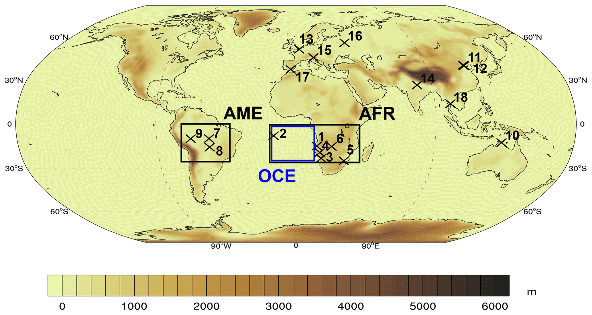
Figure 1Orography (m) used in ARPEGE-Climat simulations. Locations of the Aerosol Robotic Network (AERONET) stations used in this study are shown (black crosses; see Table 1 for details on these AERONET stations), as the different regions used in this study, AME (70–20∘ W/0–25∘ S) and AFR (15∘ W–40∘ E/0–25∘ S, black boxes) and OCE (15∘ W–10∘ E/0–25∘ S, blue box).
The ARPEGE-Climat global climate model includes the SURFace EXternalisée (SURFEX) modeling platform in its version 8 to simulate surface state variables and fluxes at the Earth's surface (Decharme et al., 2019). Over the land surface, the Interaction Soil‐Biosphere‐Atmosphere (ISBA, Noilhan and Mahfouf, 1996) land surface model and the Total Runoff Integrating Pathways (CTRIP, Decharme et al., 2019; Voldoire et al., 2019) river model are used to represent physical processes. Lastly, the ARPEGE-Climat model includes an interactive aerosol scheme described in the following paragraph.
2.2 The TACTIC aerosol scheme
TACTIC is the bulk-bin aerosol scheme used in the climate models of CNRM (Michou et al., 2015; Nabat et al., 2015), originally derived from the ECMWF IFS aerosol module (Morcrette et al., 2009; Rémy et al., 2019) and representing the main tropospheric aerosol types and their interactions with the climate. The version used in the present study is based on the one used in the CNRM-ESM2-1 simulations (Séférian et al., 2019) carried out for the sixth phase of the Coupled Model Intercomparison Project (CMIP6) and described in detail in Michou et al. (2020). Compared to the latter, TACTIC here includes the representation of nitrate and ammonium particles as described by Drugé et al. (2019), modifications on sea-salt emissions described in Nabat et al. (2020), as well as further developments described thereafter concerning the formation of sulfate particles, the aerosol wet deposition, and the aerosol–radiation coupling.
In summary, the TACTIC aerosol scheme simulates the physical evolution of seven aerosol types that are supposed to be externally mixed: desert dust, sea salt, black carbon, organic matter, sulfate, and recently added nitrate and ammonium particles. Terrestrial biogenic SOA are not formed explicitly but are taken into account through the climatology of Dentener et al. (2006), while oceanic biogenic SOA and aromatic SOA are not yet considered. To represent the particle size spectrum, the TACTIC aerosol scheme includes 16 prognostic variables or aerosol bins: three size bins are used for desert dust (DD; the respective limit diameters of the three bins are 0.01 to 1.0, 1.0 to 2.5, and 2.5 to 20 µm) and sea salt (SS; the respective limit diameters of the three bins are 0.01 to 1.0, 1.0 to 10.0, and 10.0 to 100.0 µm), two bins separating hydrophilic and hydrophobic particles for organic matter (OA) and black carbon (BC), one size bin for sulfate (SO4) particles, and another one for sulfate precursors, notably sulfur dioxide (SO2). Finally, nitrate particles (NO3) are divided into two bins (for gas-to-particle reactions and for heterogeneous chemistry), and the last two tracers are used for ammonium (NH4) and ammonia (NH3). Aerosols can be interactively emitted from the surface (DD or SS) as a function of surface wind and soil characteristics, or the scheme can consider external emission data sets, including those for anthropogenic and/or biomass burning particles (BC, OA, SO2, and NH3). As described in Michou et al. (2015), a multiplier coefficient of 1.5, based on analysis of fresh urban emissions (Turpin and Lim, 2001), is applied to organic carbon emissions in order to take into account the conversion of organic carbon into organic matter.
In TACTIC, the formation of sulfate was originally based on the conversion of sulfate precursors (summarized as SO2) into sulfate assuming an exponential decay with a time constant depending on the latitude (Rémy et al., 2019). In the present version, the sulfate formation now deals explicitly with the chemical oxidation of sulfate precursors into sulfate. Three oxidants are taken into account: OH in the gas phase and H2O2 and O3 in the aqueous phase. The chemical mechanism is derived from that of Berglen et al. (2004), with updated reaction rates (Seinfeld and Pandis, 2006; Burkholder et al., 2015) and updated Henry's law solubility coefficients (Sander, 2015). The concentrations of the oxidants consist of monthly climatologies built from diagnostics of the CAMSiRA global reanalysis of atmospheric composition (Flemming et al., 2017).
The modifications in the aerosol wet deposition scheme consist in considering together the sum of large-scale and convective precipitation to scavenge aerosols with this resulting precipitation flux and in refining the representation of the in-cloud scavenging according to the type of cloud. Indeed, the in-cloud scavenging, which represents most of the total scavenging, is not the same for liquid, mixed-phase, and solid clouds. TACTIC now uses specific coefficients for these three types of clouds, based on those proposed by Bourgeois and Bey (2011). The resuspension of aerosols when precipitation evaporates has also been improved, using a correction factor described in de Bruine et al. (2018). Finally, a mass fixer is now applied to ensure conservative tracer transport (Bermejo and Conde, 2002).
The atmospheric model represents the interactions between particles and radiation (aerosol direct effect) and between particles and cloud albedo (first aerosol indirect effect; see Michou et al., 2020, for details). On the other hand, the second indirect aerosol effect, which corresponds to interactions between aerosols and cloud precipitation, is not included for the time being. With regards to aerosol–radiation interactions, TACTIC is able to produce different aerosol optical properties (extinction, SSA, and asymmetry parameter; see Table A1) for the wavelengths of the radiation scheme, based on look-up tables pre-calculated using a Mie code and the aerosol sphericity hypothesis (Ackerman and Toon, 1981) (see Table A2 for references of the refractive indices). These properties depend on the relative humidity, except for DD and hydrophobic BC and OA. In this version of ARPEGE-Climat, the interaction between aerosols and radiation has been improved, and the radiative code is provided with all aerosol optical properties for each aerosol bin and each wavelength in both the shortwave and longwave spectra.
Finally, it is worth mentioning that the TACTIC aerosol scheme keeps a reasonable computation cost, notably thanks to several simplifications such as not calculating online the aerosol optical properties or not interacting with gaseous tropospheric chemistry.
2.3 Brown carbon implementation
A new prognostic aerosol species has been added to the TACTIC aerosol scheme: the BrC. The first step of this implementation, which allows for a good representation of the spatial and temporal variability of the BrC absorption, consisted in separating BrC from OA according to their sources. To do this, OA emissions were separated into three sources: BB, fossil fuel (FF), and BF as presented in Fig. 2. Included in the model BB emissions, provided over the 2000–2014 period, are those described in van Marle et al. (2017) with the GFED4s (Global Fire Emissions Database) as an anchor data set. Then, BF emissions mainly come from the residential, industry, and energy sectors, and FF emissions are those of the CEDS (Community Emissions Data System) inventory released for CMIP6 (Hoesly et al., 2018). In this parameterization, BrC corresponds to organic aerosols emitted by BB and BF, while OA correspond to organic aerosols emitted by FF. At this stage, we consider our OA aerosol to be a non-absorbing aerosol, as shown by most observations (Laskin et al., 2015), while BrC is considered to be an absorbing aerosol.
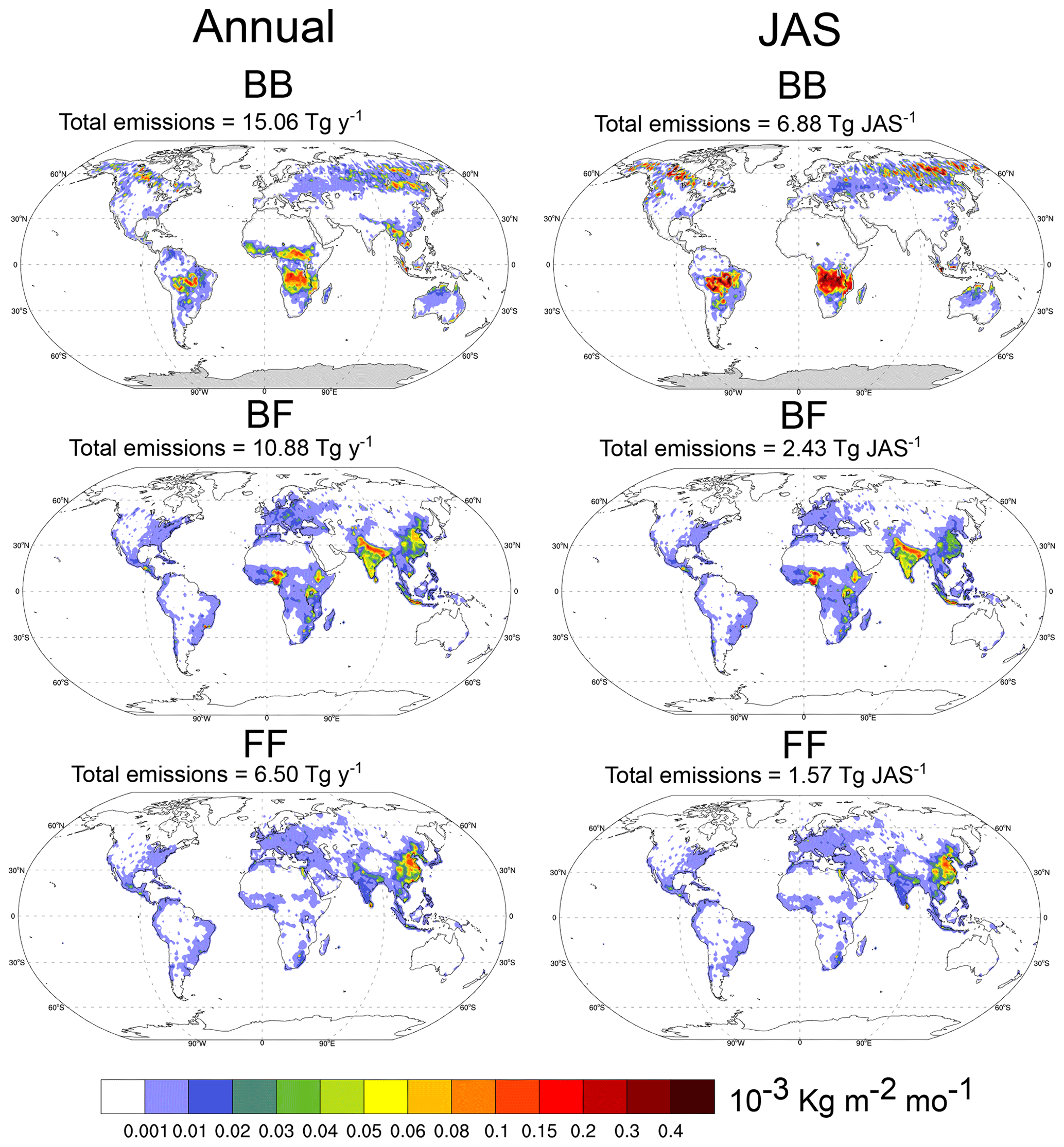
Figure 2Annual and JAS biomass burning (BB), biofuel (BF), and fossil fuel (FF) organic carbon emissions (10−3 kg m−2 mo−1, 2000–2014 average). BB and BF emissions correspond to BrC emissions in the BRC_NOBL and BRC model runs. Total BB emissions (Tg) in the period are given on top of each panel.
The second step of this implementation work was therefore to calculate the BrC optical properties at different wavelengths and different relative humidity using a Mie code (Toon and Ackerman, 1981). For this purpose, we used the BrC refractive index (RIBrC) shown in Eq. (1): the real part (1.53) is the one commonly used in previous studies (Chen and Bond, 2010; Arola et al., 2011; Lin et al., 2014; Tuccella et al., 2020) and remains close to that used in the model for OA (1.45), while the imaginary part comes from experimental results (Saleh et al., 2014):
The imaginary part depends on the BC-to-OA ratio from BB and BF emissions. Its wavelength (λ) dependence is further detailed in Eq. (2). As in other climate models, we chose to use a constant global BC-to-OA emission ratio. It is therefore important to note that this assumption does not reflect all burning conditions and specific fires (Andreae, 2019). Wang et al. (2018) fixed a global average BC-to-OA emission ratio for each source (0.12 for BF and 0.05 for BB) and indicate that the variability of the BC-to-OA ratio (0–0.23 for BF and 0.03–0.06 for BB in the GFED4s emission inventory) is underestimated because not all of the burning conditions are represented. This is reinforced by Ramo et al. (2021), who show that, since the 1990s in sub-Saharan Africa, burned area and fire carbon emissions are underestimated because they are strongly impacted by small fires, which are undetected by coarse-resolution satellite data. Brown et al. (2018) ran a sensitivity experiment with a BC-to-OA ratio set to 0.08, and based on their results we adopted this ratio. The BrC geometric median diameter is assumed to be 0.2 µm (Saleh et al., 2015) with a standard deviation of 1.6 (Wang et al., 2018; Tuccella et al., 2020). The density of BrC, usually ranging from 1 to 1.5 (Feng et al., 2013; Lin et al., 2014; Shamjad et al., 2016; Wang et al., 2018; Tuccella et al., 2020), is assumed to be 1 g cm−3 as in the study of Brown et al. (2018).
We implemented a BrC bleaching parameterization represented by the passage from a hydrophobic bin to a hydrophilic bin, each having specific optical properties, the hydrophilic bin absorption being lower than that of the hydrophobic bin. The passage is done with a characteristic time of 1 d. This characteristic time ranges from a few minutes to several days in the literature (Zhong and Jang, 2011; Lee et al., 2014; Forrister et al., 2015; Zhao et al., 2015; Wang et al., 2016; Vakkari et al., 2018; Zhang et al., 2020), but 1 d is commonly used (Wang et al., 2016; Brown et al., 2018; Wang et al., 2018). Then, knowing that the level of BrC absorption decrease over time reaches up to 75 % of the initial absorption in certain studies (Wang et al., 2018; Zhang et al., 2020), we tested several absorption decreases (25 %, 50 %, and 75 %). The best comparison to our reference data sets was obtained with the 50 % value. For clarity reasons, we decided to show here only results with the 50 % value. The aerosol scheme can also be run without BrC aging. In this case, BrC is only represented by one hydrophilic variable. The different BrC optical properties are summarized, at 350 and 550 nm, in Table A1 for a relative humidity of 0 % and 80 %. A BrC dry deposition velocity of 0.1 cm s−1, close to the first SS and DD bin deposition velocity (Michou et al., 2015), is set over all surfaces (ocean, sea ice, land, and land ice). Lastly, the efficiency with which BrC particles are washed out is 0.001 for rain and 0.01 for snow (below-cloud scavenging, Michou et al., 2015), while the fraction of BrC included in a cloud droplet is 0.25 (0.20 for the hydrophobic bin) for liquid clouds and 0.06 for mixed-phase and ice clouds (in-cloud scavenging, Bourgeois and Bey, 2011). For reasons of consistency, and awaiting further studies, these values are the same as those used for OA aerosols.
One limitation of this study is to neglect absorption by biogenic (Lin et al., 2014; Saleh et al., 2015) and aromatic SOA (Wang et al., 2014; Jo et al., 2016; Wang et al., 2018). Some studies show that the absorption of the primary BrC from BB and BF emissions usually dominates that of the absorbing SOA (Saleh et al., 2013; Martinsson et al., 2015; Wang et al., 2016). However, Kumar et al. (2018) indicate in their study that SOA, after aging, can contribute significantly to the overall absorption.
3.1 Reference data sets
In this study, different data sets have been used to evaluate the ability of the ARPEGE-Climat model to reproduce the total absorption aerosol optical depth (AAOD), single-scattering albedo (SSA), and aerosol optical depth (AOD). First, given their spatial and temporal scales, four satellite products have been used to provide estimates of the total AAOD and SSA (at 350 and/or 440 nm) and of the total AOD (at 550 nm).
-
PARASOL-GRASP (2006–2012, 1∘ resolution, Chen et al., 2020) for the AAOD and SSA at 440 nm and the AOD at 550 nm. This satellite product, initially developed by the science team at LOA (Laboratoire d'Optique Atmosphérique, Lille, France), is obtained by the Generalized Retrieval of Atmosphere and Surface Properties (GRASP) algorithm from POLDER-PARASOL observations. The GRASP algorithm, described in Dubovik and King (2000) and Dubovik et al. (2011, 2014), was developed to derive extensive aerosol properties from a variety of remote sensing instruments. In this study, version 2.1 L3 of the PARASOL-GRASP “models” configuration is used. The AAOD or AOD uncertainty does not exceed 0.01 (0.02 for SSA and AOD over the ocean) at all wavelengths (Chen et al., 2020). SSA values are aggregated only when AOD (443 nm) is greater than or equal to 0.3 over land and 0.02 over the ocean. This very low threshold (0.02) for filtering SSA over the ocean was chosen in order to retain a sufficient number of SSA and AOD retrievals (Chen et al., 2020).
-
OMI-OMAERUVd (2005–2019, 1∘ resolution, Torres et al., 2007, 2013) for the AAOD and SSA (350 and 440 nm) and the AOD (550 nm). The OMI (Ozone Monitoring Instrument) OMAERUVd data set comes from a spectrometer aboard NASA’s Earth Observing System’s Aura satellite and is archived at the NASA Goddard Earth Sciences Data and Information Services Center. The level-3 daily global gridded product OMAERUVd-v003, used in this study, is produced with all data pixels which fall in a grid box with the quality-filtered data product OMI Level-2 Aerosol OMAERUV based on the pixel level. The OMAERUV data product is an improved version of the TOMS version-8 algorithm that essentially uses ultraviolet radiance data (Jethva et al., 2014). The estimated uncertainty in retrieved SSA is ±0.03 for AOD (440 nm) larger than 0.4. This error is largely attributed to the uncertainty in the instrument calibration (Dubovik et al., 2000; Jethva et al., 2014). AOD over land is expected to have the same root mean square error (RMSE) as TOMS retrievals (0.1 or 30 %, whichever is larger). Over the ocean, the AOD RMSE is likely to be 2 times larger. The RMSE for AAOD is estimated to be 0.01 (OMI User’s Guide). An evaluation of the OMAERUVd aerosol SSA data through comparisons against daily SSA products from 541 globally distributed AERONET stations for a 15-year period (2005–2019) was carried out in the study of Drakousis et al. (2020). They show that about 50 % of OMI-OMAERUVd–AERONET matchups agree within the absolute difference of 0.03 at 440 nm. However, they also indicate that OMI-OMAERUVd tends to overestimate SSA over areas where biomass burning occurs.
-
MACv2 (2001–2016 with the reference year 2005, directory spectral/ssp_31bands, 1∘ resolution, Kinne, 2019) for the AAOD and SSA (350 and 440 nm) and the AOD (550 nm). The Max Planck Institute Aerosol Climatology (MACv2) is an update of the MAC-v1 climatology described in Kinne et al. (2013). This data set provides monthly aerosol optical properties derived from a combination of observations, like those from the AERONET and MAN (Marine Aerosol Network, Smirnov et al., 2009) ground networks, and model outputs derived from the AeroCom global modeling initiative (Kinne et al., 2006; Koffi et al., 2016). The interannual variability is taken into account through an AOD change for the anthropogenic aerosols, but only monthly variations are used for natural aerosols. The AAOD uncertainty is estimated at about 0.003.
-
FMI_SAT (1995–2017, 1∘ resolution, Sogacheva et al., 2020) for the AOD at 550 nm. FMI_SAT is the name given to the merged AOD product presented in Sogacheva et al. (2020). This product, which provides AOD monthly data, was built from 12 individual satellite products and evaluated with the AERONET ground network. It provides AOD data with an uncertainty reaching 0.006 on average and up to 0.05 in regions with high AOD (Sogacheva et al., 2020).
Table 1Characteristics of the AERONET stations used in this study: station name, location, altitude, the number of months available over at least 3 years during the observation period (2000–2020), and the total year/JAS available over the observation period (2000–2020).

Second, we considered AERONET (from 2000 to 2020 depending on the station, Holben et al., 1998) data. This network consists of globally distributed ground-based Sun photometers which provide local column-integrated aerosol properties at different solar wavelengths, including 440 nm. The column extinction Ångström exponent can be directly calculated from the wavelength-dependent AOD measurements (Eck et al., 1999). In this study, monthly average data (version 3, level 1.5 with an automated cloud screening, Smirnov et al., 2000) have been used. A complete description of the version-3 AERONET product is available in Sinyuk et al. (2020). Unlike level 2.0 (quality-assured data), level 1.5 reports 440 nm AAOD and SSA for all AODs, including AOD lower than 0.4 (Lacagnina et al., 2015). For comparison to our model results, AAOD and SSA data at 440 nm were directly used. It should be noted that 440 nm is the shortest available wavelength in AERONET data. We calculated AOD at 550 nm using the Ångström coefficients provided. AERONET uncertainties have been reported in several papers. Eck et al. (1999) and Kinne et al. (2013) indicate that the AOD and AAOD uncertainties are approximately 0.01. Concerning the SSA, Dubovik et al. (2000) report an uncertainty of 0.03. However, it should be noted that larger SSA uncertainties are expected at low AODs (Lacagnina et al., 2015). In order to have the most accurate comparison to the model, we decided to keep only AERONET monthly data with at least eight daily values to derive the mean of each month, and for a given month we keep only the stations with at least three monthly values over the 2000–2020 period. In the end, we selected 18 stations: 6 in Africa, 3 in South America, and 9 in Europe and Asia, as shown in Fig. 1 (see also Table 1).
It can be noted that a global representation of the spectral aerosol absorption in the UV-to-visible wavelength range (340–670 nm) based on a synergy of ground measurements (AERONET AOD) and satellite observations (near-UV OMI radiances and visible MODIS (Moderate-Resolution Imaging Spectroradiometer) radiances) is presented in Kayetha et al. (2022).
Table 2Summary of the main characteristics of the reference data sets used in this study.
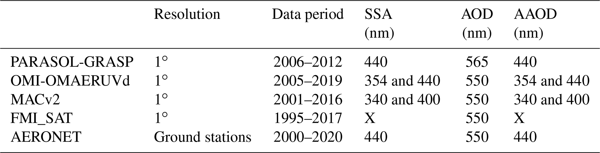
Lastly, it is important to mention that the satellite data sets, as well as the AERONET data, were obtained during daytime only, in contrast to the model data, which were obtained over the whole day (night plus day). The main characteristics of the reference data sets described here are summarized in Table 2.
3.2 Simulations
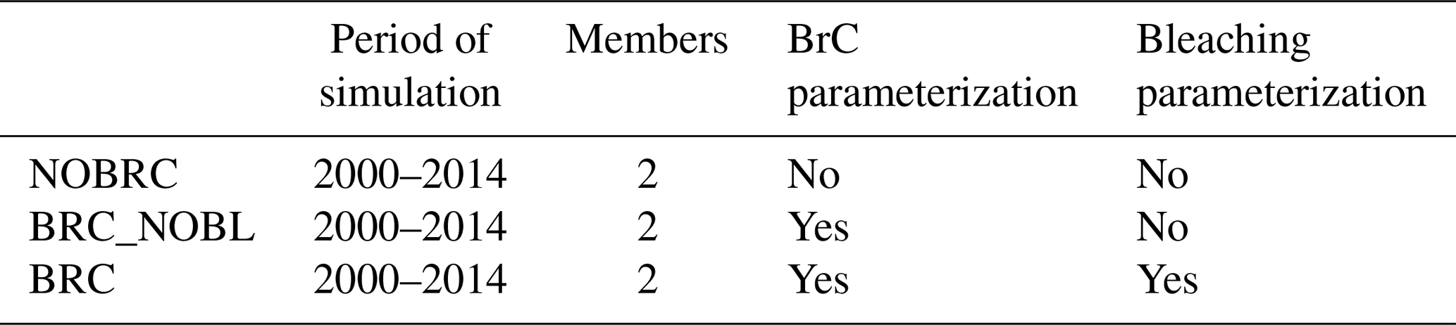
Two main configurations of the aerosol scheme have been used in this study, with or without BrC aerosols. All simulations consist of 30-year AMIP-type simulations with prescribed monthly sea surface temperature (SST) and sea ice fraction. The period covered is 2000–2014; it is simulated twice for each simulation (by changing the initial state of the atmosphere), so the total number of simulated years is 30. The simulation defined as the baseline for this work, using ARPEGE-Climat without the BrC parameterization, is called NOBRC. The second simulation, called BRC, differs from NOBRC as it considers a new BrC tracer as well as a bleaching parameterization. For a sensitivity study, an additional simulation, named BRC_NOBL, has been performed. This third simulation considers the new BrC tracer but does not take into account the bleaching parameterization. The main characteristics of these three simulations are summarized in Table 3.
Table 3Summary of the main characteristics of the three simulations used in this study.
For information, multiplier coefficients of 1.7 (simulations with BrC) or 1.8 (simulations without BrC), in addition to the first multiplier coefficient of 1.5 presented in Sect. 2.2, have been applied to particulate aerosol (OA and BC) biomass burning emissions, as done in other studies (e.g., Kaiser et al., 2012). These coefficients (1.7 and 1.8) are based on an AOD (550 nm) comparison between that simulated by the model (2000–2014) and that provided by the merged AOD product FMI_SAT (1995–2017, described below) over regions influenced by large biomass burning emissions (10–40∘ E/0–15∘ S over Africa and 40–70∘ W/0–20∘ S over South America). This comparison was performed over the months of July, August, and September (JAS), which is the period with the most intense biomass burning activity over the tropics. The objective of these coefficients was to ensure a similar regional JAS total AOD between simulations and FMI_SAT.
3.3 Effective radiative forcing calculation
A forcing concept, which allows all physical variables to respond to perturbations except those about the ocean and sea ice, was introduced by Myhre et al. (2013) and Shindell et al. (2013): the ERF. In order to estimate the BrC ERF, we used the method recommended in Ghan (2013). In this method, the total ERF can be differentiated between aerosol–radiation interactions (ERFari), aerosol–cloud interactions (ERFaci), and a residual term representing mainly surface-albedo changes (ERFres).
In Eq. (4), Δ refers to the difference between the simulation with (BRC) and the simulation without (NOBRC) BrC aerosols. The F variable represents the TOA net radiation flux (SW + LW), and Fclean refers to the TOA net radiation flux (SW + LW) neglecting both aerosol scattering and absorption. Then, in Eq. (5), Fclear,clean is the clear-sky fluxes when neglecting both aerosol scattering and absorption. Other methods of calculating ERFari and ERFaci exist, but the Ghan (2013) technique seems to be particularly accurate (Zelinka et al., 2014). It is important to note here that the BrC indirect effect is taken into account in the same way as the OA aerosol indirect effect.
4.1 Evaluation of the aerosol scheme
4.1.1 Local scale
Firstly, ground-based AERONET observations are used to locally evaluate the ARPEGE-Climat simulations. Figures 3, 4, and A1 present, respectively, the SSA (440 nm, 400 nm for MACv2), the AAOD (440 nm, 400 nm for MACv2), and the AOD (550 nm, 565 nm for PARASOL-GRASP) annual cycles at the selected AERONET sites (linear interpolation at the station point), simulated by the ARPEGE-Climat model (NOBRC, BRC_NOBL, and BRC simulations) and retrieved by AERONET as well as by our other reference products (PARASOL-GRASP, OMI-OMAERUVd, MACv2, and FMI_SAT). As a reminder, as described in Sect. 3.2, the AOD (550 nm) is tuned in each simulation to be as consistent as possible with the merged AOD product FMI_SAT. The 550 nm wavelength was chosen for the AOD evaluation as we could not identify reference satellite products at other wavelengths of the same quality as FMI_SAT. It is interesting to note here that the different satellite products (see Table 2 for reference data set details) are not always very consistent with the AERONET data, both in annual cycle and in annual average. Over regions with high biomass burning activity such as southern Africa and South America, Figs. 3 and 4 indicate a decrease (increase) in SSA (AAOD) for simulations including BrC at all AERONET stations, particularly during the JAS period. These figures also show that these changes are even more pronounced with BRC_NOBL. Conversely, Fig. A1 shows a very small BrC impact on total aerosol AOD; indeed, the three simulations show similar values at all AERONET stations. In more detail, Fig. 3 shows SSA BRC and BRC_NOBL SSA, in better agreement with the different observation data sets at all stations over Africa and South America than NOBRC SSA. The bleaching parameterization allows us, at some AERONET stations, to better represent the observations (e.g., HESS, Windpoort, or Skukuza). However, at other AERONET stations (e.g., Lubango, Ascension_Island, and Mongu Inn), the BRC_NOBL simulation seems to show results in better agreement with the observations. At Windpoort or Skukuza, Fig. 3 shows a SSA decrease of about 0.05 with the BRC simulation during the summer period, which is consistent with the SSA decreases shown by all observation data sets. At Mongu Inn, there is a stronger SSA decrease of 0.08 associated with an AAOD increase of 0.06 over the JAS period between the NOBRC and BRC_NOBL simulations. BRC_NOBL is therefore the closest to the AERONET observations. As for the SSA, the BrC implementation allows us to simulate AAOD close to all observations. Indeed, Fig. 4 shows that AAOD is systematically underestimated with the NOBRC simulation, both over African and South American stations. Nevertheless, when the bleaching parameterization is not taken into account (BRC_NOBL), AAOD is often slightly overestimated (up to 0.03 during JAS) compared to all observations. On the other hand, the BRC simulation shows lower AAOD values than the BRC_NOBL simulation, and this sometimes results in underestimated AAODs at some sites (e.g., Lubango or Mongu Inn). Over Europe and Asia (AERONET stations grouped under “Other”), Figs. 3 and 4 show that the BrC implementation has a very small impact on the total SSA and AAOD, as in these regions the BrC AOD represents less than 7 % of the total aerosol AOD. However, Figs.3 and 4 show with the BrC implementation a SSA decrease and an AAOD increase at some Asian stations such as Jabiru (northern Australia) (−0.05 for SSA and +0.01 for AAOD during summer and fall) or Beijing and XiangHe (China), with an AAOD increase (+0.01) during spring.
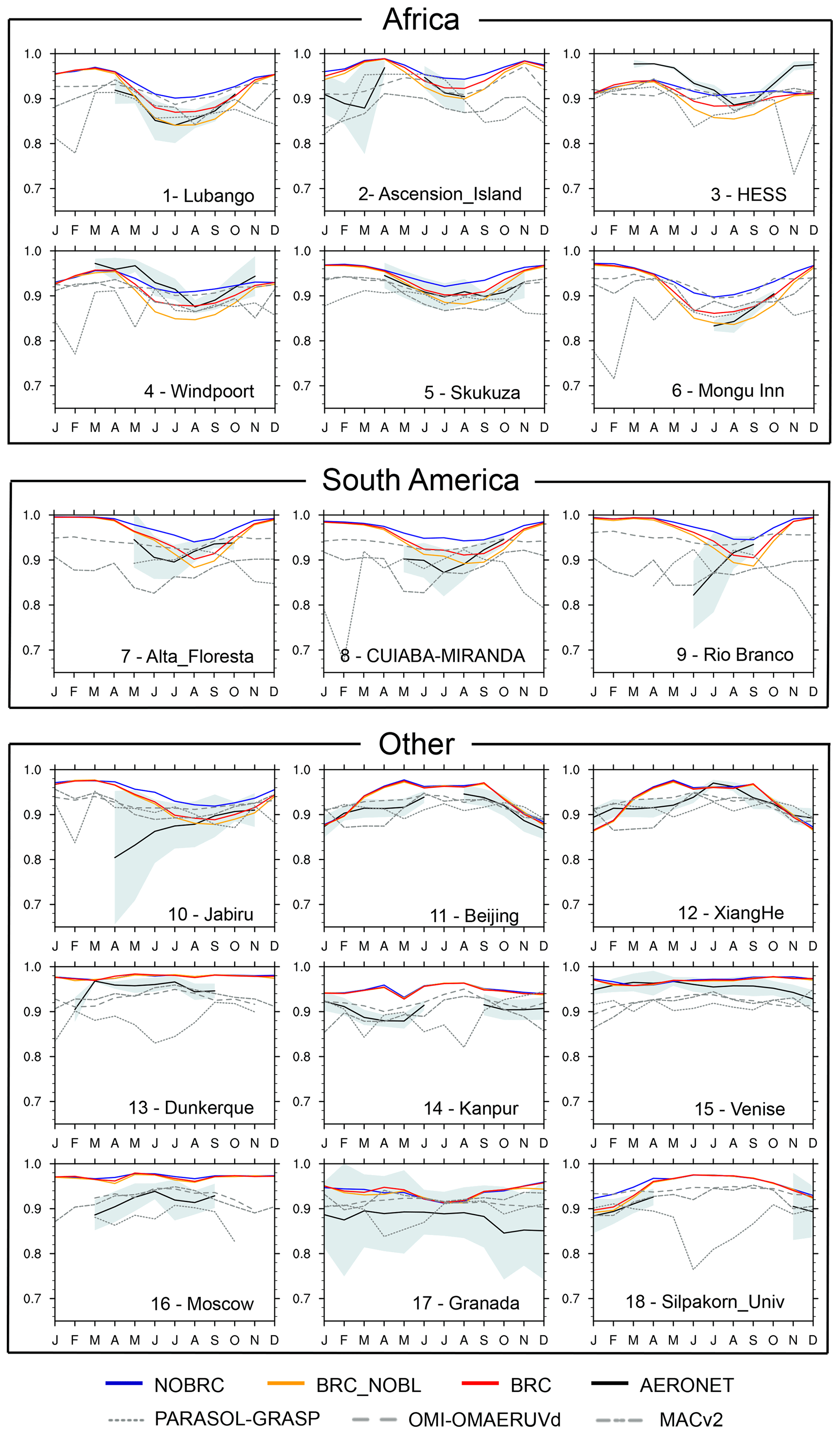
Figure 3Annual cycle of the SSA (440 nm) at AERONET stations, simulated by the ARPEGE-Climat model for the NOBRC (blue), BRC_NOBL (orange), and BRC (red) simulations (see Table 3 for details), with AERONET measurements (black, plus or minus standard deviation in light blue), and provided by the reference data sets (grey) with PARASOL-GRASP, OMI-OMAERUVd, and MACv2 (see Table 2 for details). Stations have been grouped into African ones, South American ones, and stations over the rest of the world (label “Other”). AERONET stations are detailed in Table 1.
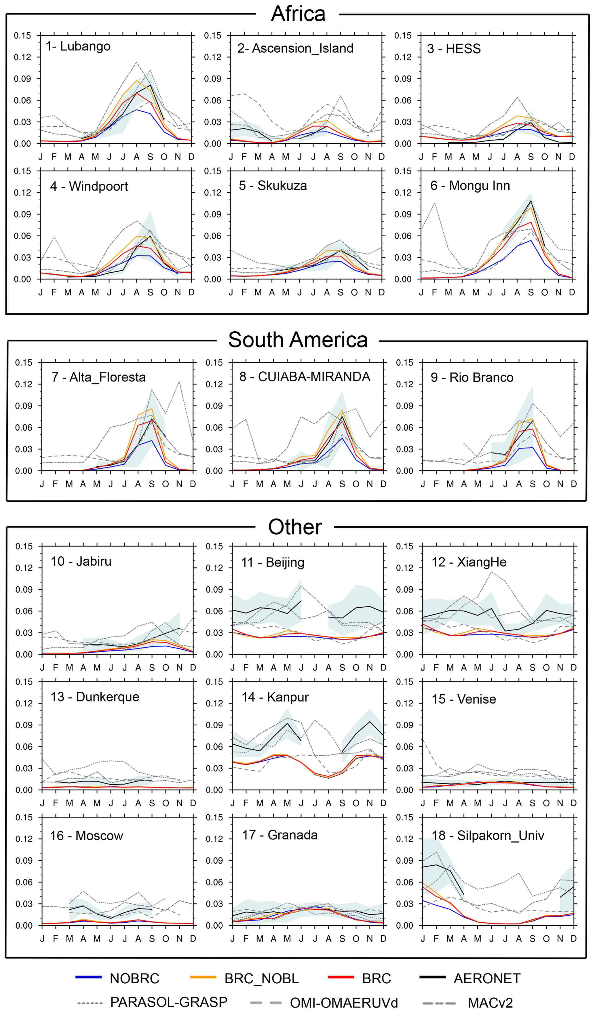
Table 4SSA (440 nm), AAOD (440 nm), and AOD (550 nm) JAS averages simulated with the NOBRC, BRC_NOBL, and BRC simulations and provided by reference data sets (PARASOL-GRASP, OMI-OMAERUVd, MACv2, and FMI_SAT; see Table 2 for details). Means ±2σ (significance level of 95 %) values interpolated at the station location (see Table 1) are given.
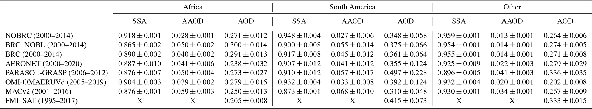
For the sake of clarity, SSA, AAOD, and AOD averages over the JAS period are summarized in Table 4. On average over all African AERONET stations, the BRC simulation presents a mean SSA equal to 0.890 ± 0.002, which is in better agreement with the range of the observations (0.876 ± 0.007–0.904 ± 0.003) than that of the NOBRC simulation (0.918 ± 0.001) and that of the BRC_NOBL simulation (0.865 ± 0.002). Over these stations, the total aerosol AAOD simulated by NOBRC is equal to 0.028 ± 0.001 against 0.040 ± 0.002 for the BRC and 0.050 ± 0.002 for the BRC_NOBL simulations. Compared to the different reference data sets showing an AAOD between 0.039 ± 0.002 and 0.059 ± 0.003, the NOBRC simulation therefore underestimates observations, in contrast to the BRC and BRC_NOBL simulations. Table 4 shows similar results for the South American AERONET stations with a simulated SSA (0.917 ± 0.008 and 0.900 ± 0.008) and AAOD (0.045 ± 0.012 and 0.055 ± 0.012) with the BRC and BRC_NOBL simulations, respectively, which fall within the range of the different reference data sets (0.873 ± 0.001–0.932 ± 0.004 for SSA and 0.033 ± 0.008–0.068 ± 0.010 for AAOD), contrary to the NOBRC simulation (0.948 ± 0.004 for SSA and 0.027 ± 0.006 for AAOD). Over the African AERONET stations, Table 4 indicates that AOD from BRC and BRC_NOBL is slightly higher (0.300 ± 0.014 and 0.291 ± 0.013, respectively) than our reference range (0.205 ± 0.008–0.279 ± 0.015). However, over South American AERONET stations, BRC and BRC_NOBL AOD are within this range. Finally, as previously discussed, Table 4 shows only little differences between the three simulations at the European/Asian AERONET stations, except for slightly lower SSA and slightly higher AAOD for the BRC and BRC_NOBL simulations, closer then to the reference data sets.

Figure 5Boxplots of various biases compared to the AERONET observations, over the year (a, c) and over JAS (b, d). SSA (440 nm, a, b) and AAOD (440 nm, c, d). Simulations: NOBRC, BRC_NOBL, and BRC (see Table 3 for details) and reference data sets (PARASOL-GRASP, OMI-OMAERUVd, MACv2; see Table 2 for details). Uncertainty of the AERONET observations appears shaded.
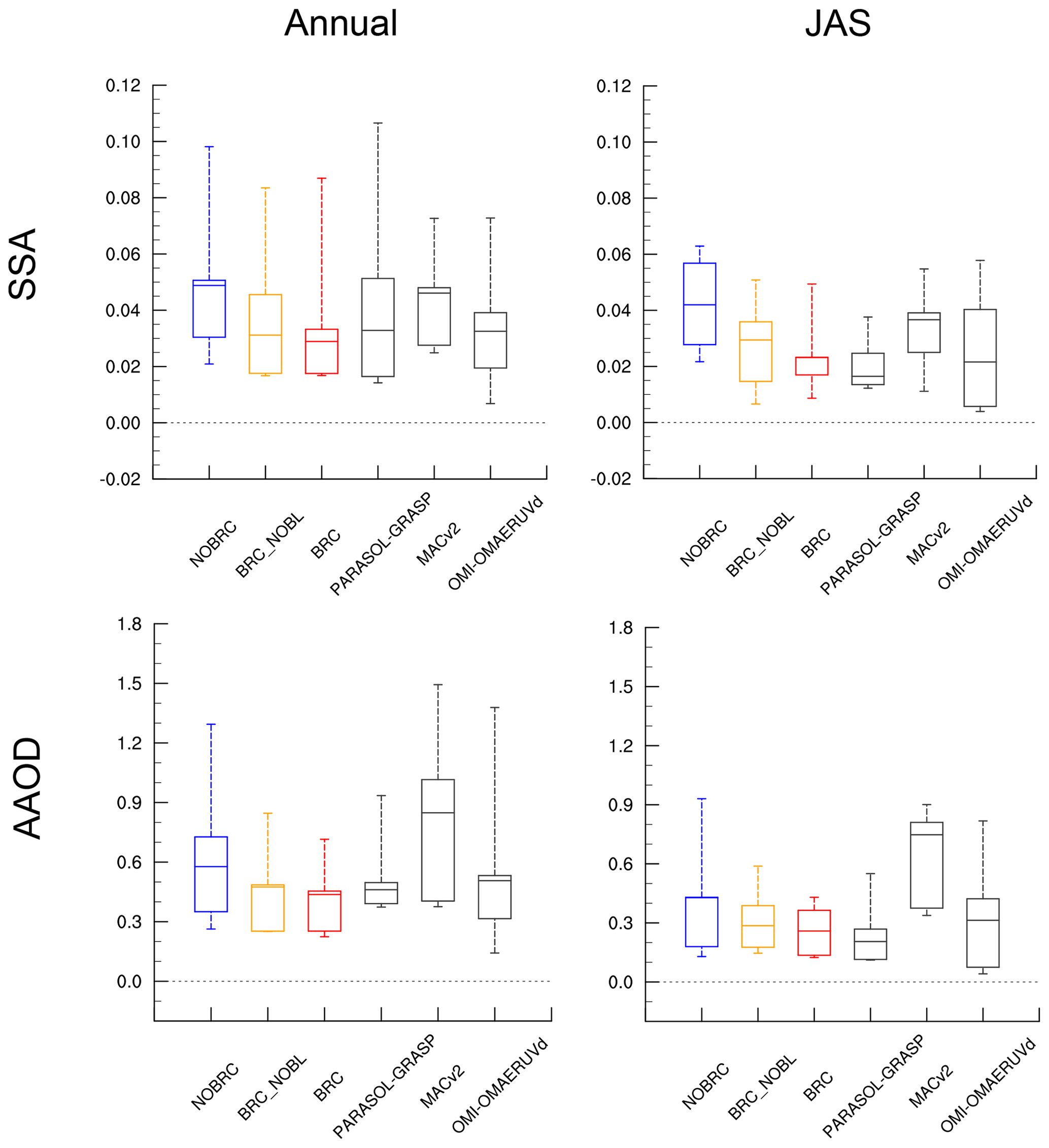
Biases and normalized root mean square error (NRMSE, defined as the ratio between the RMSE and the average of the AERONET data) boxplots between observed (average of the African and South American AERONET stations) and predicted SSA and AAOD are presented in Figs. 5 and 6 (see Fig. A2 for the AOD). These figures clearly show a decrease in bias and NRMSE of SSA and AAOD with the BrC implementation in both annual and JAS statistics. The most marked improvement occurs when the bleaching parameterization is taken into account (BRC simulation): the median SSA bias is reduced from 0.025 (annual) and 0.035 (JAS) in the NOBRC simulation to almost zero in the BrC simulation. If the bleaching is not taken into account (BRC_NOBL simulation), the median SSA bias is −0.015 annually and −0.020 over JAS. Figure 5 also shows similar results for the AAOD, with a strong reduction in the bias with the BRC simulation to reach very low values in both annual and JAS statistics. However, Fig. A2 shows a slight increase in the median AOD bias (+0.010 annually and +0.020 over JAS) and NRMSE (+0.100 annually and +0.050 over JAS) with the BrC implementation. The different diagnostics presented in this section therefore show a significant SSA and AAOD improvement thanks to the BrC parameterization, and this betterment is even clearer when the BrC bleaching parameterization is also taken into account. For clarity reasons, only the NOBRC and BRC simulations will therefore be presented in the remainder of this study.
4.1.2 Global scale
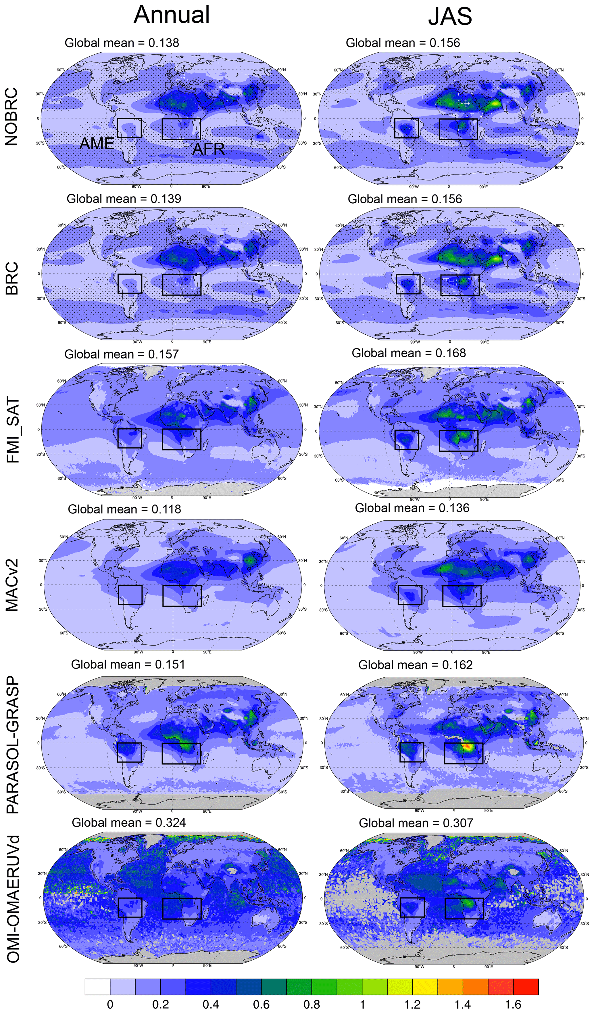
Simulated SSA, AAOD, or AOD from the two model simulations, without BrC and with BrC and its bleaching parameterization, are now compared in a climatological perspective to several monthly satellite products. We performed these comparisons globally and over regions influenced by large biomass burning emissions, namely the AFR region (AFRica, 15∘ W–40∘ E/0–25∘ S) and the AME region (South AMErica, 70–20∘ W/0–25∘ S) (see Fig. 1). Over these regions, Fig. 7 presents the absorption of the different aerosols at 350, 440, and 550 nm simulated with the BRC simulation. This figure shows an important BrC absorption comparable to that of BC at short wavelengths, especially during the JAS period. In detail, BrC absorption is about 45 % of BC absorption at 350 nm and about 35 % at 440 nm. These results are consistent with the study of Bahadur et al. (2012) that estimates a BrC absorption at 440 nm of about 40 % of that of BC. At 550 nm, Fig. 7 shows a lower BrC absorption which is less than 30 % of that of BC. For comparison to other studies, Samset et al. (2018) show with the LMDZ-INCA model a simulated BrC AAOD at 550 nm of about 20 % of that of BC. In this section we will therefore evaluate the aerosol scheme at 350 and 440 nm, which are the wavelengths where BrC contributes most to the total absorption. Figures 8 and 9 present, respectively, the comparison of the SSA at 350 and 440 nm simulated by the model (NOBRC and BRC) to that retrieved from the MACv2, PARASOL-GRASP, and OMI-OMAERUVd data sets over the year and over JAS. All temporal and spatial averages are summarized in Table 5. The SSA clearly decreases when considering the BrC aerosol, especially during the JAS season over AFR (average decreases of 0.036 at 350 nm and 0.024 at 440 nm) and AME (average decreases of 0.025 at 350 nm and 0.019 at 440 nm). SSA is also improved at high latitudes at both 350 and 440 nm (see the white hatching over North America and Russia). One has to note that the SSA of the various reference data sets differs significantly (see also Figs. A3 and A4). Both on annual average or for the JAS season, the OMI-OMAERUVd product shows higher SSA (at least +0.04) than those observed by PARASOL-GRASP and MACv2 over AFR and AME. Previous studies have already shown differences, sometimes systematic, between AERONET and satellite data sets and also among satellite products (Schutgens et al., 2020, 2021). The NOBRC SSA during JAS, with averaged values of 0.925 ± 0.001 and 0.930 ± 0.001 at, respectively, 350 and 440 nm over AFR, is overestimated compared to all reference data sets. Table 5 also shows similar results over the AME region. The BRC simulation, characterized by an SSA of 0.889 ± 0.002 (0.906 ± 0.002) at 350 nm (440 nm) over AFR during this season, is therefore more consistent with the reference data sets, with SSA close to those measured by OMI-OMAERUVd (0.870 ± 0.003 at 350 nm and 0.914 ± 0.002 at 440 nm) and slightly higher than SSA derived by PARASOL-GRASP (0.885 ± 0.009 at 440 nm) and by MACv2 (0.826 ± 0.001 at 350 nm and 0.873 ± 0.001 at 440 nm). Similar conclusions can be derived over the AME region (see Table 5).
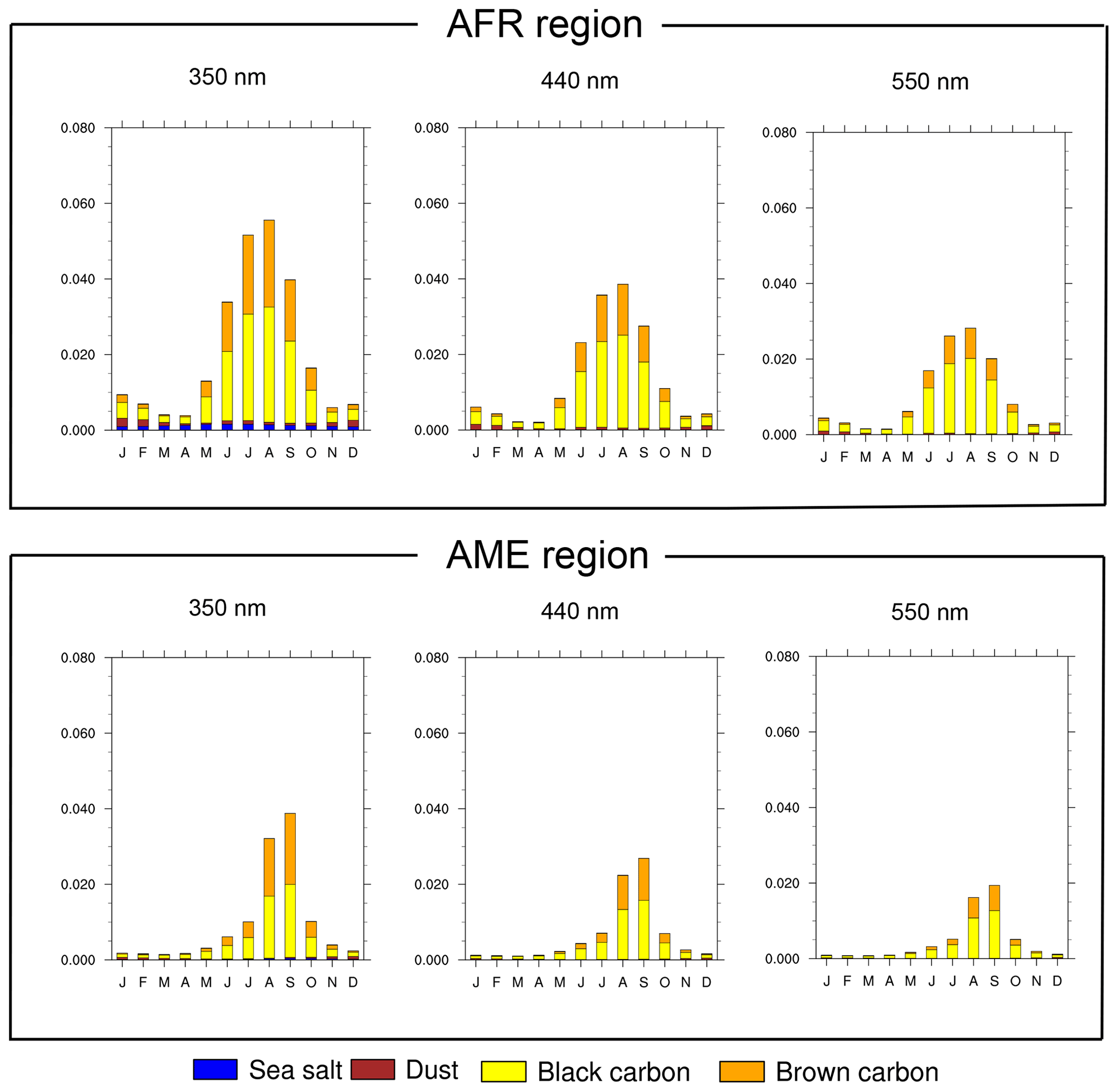
Figure 7AAOD (350, 440, and 550 nm) of the different absorbing aerosols over the AFR and AME regions (BRC simulation; see Table 3 for details).
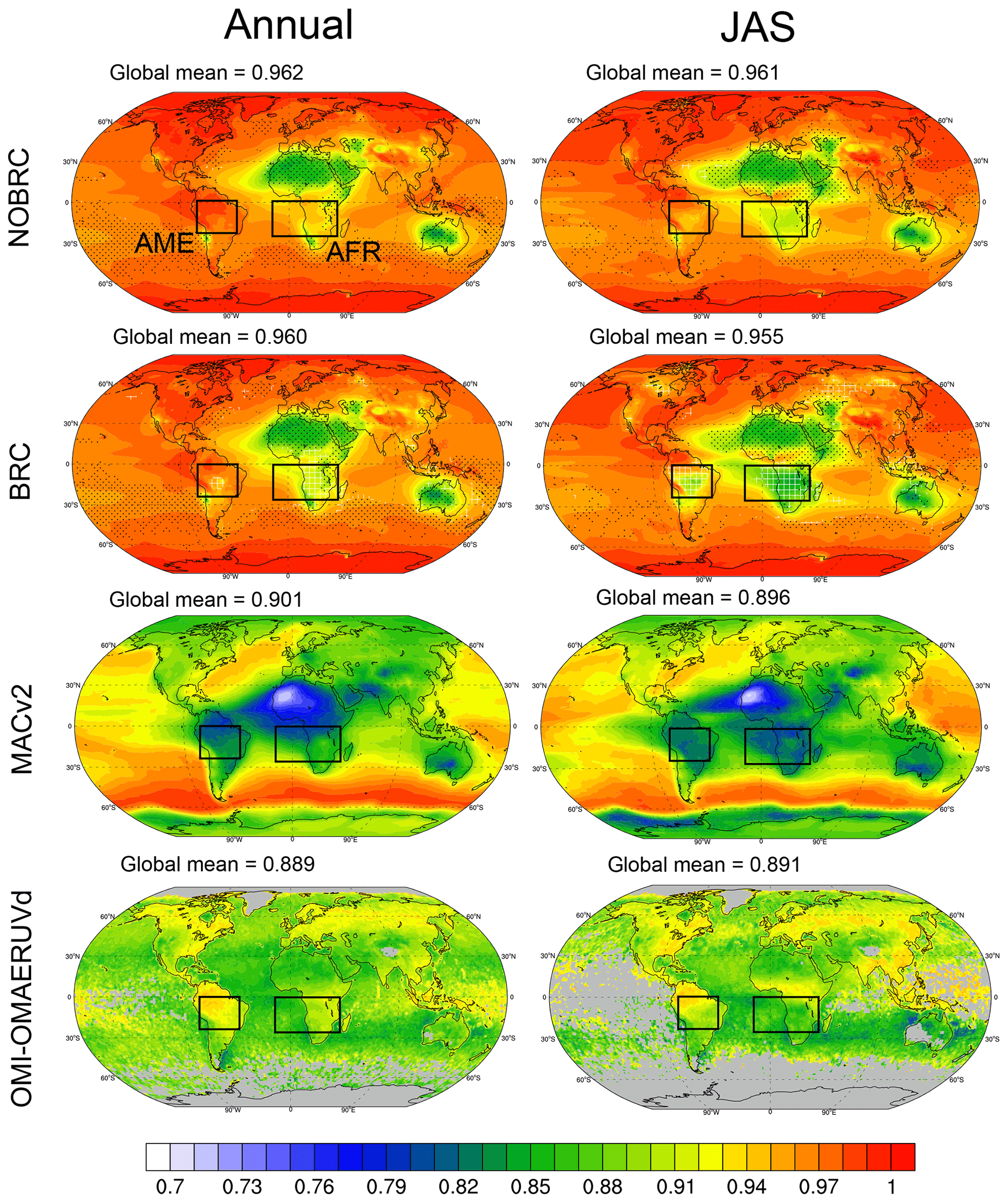
Figure 8SSA (350 nm) simulated by the ARPEGE-Climat model for the NOBRC and BRC simulations and retrieved from MACv2 and OMI-OMAERUVd (see Tables 2 and 3 for details) averaged over the year and over the months of July, August, and September (JAS). Black dots in the model plots show common locations between the NOBRC and BRC simulations where the SSA is inside the range covered by MACv2 and OMI-OMAERUVd (reference data set uncertainties included; AERONET uncertainties are used when data are not available). Changes in these locations between the NOBRC and BRC simulations are highlighted by white hatching. Shaded areas indicate a missing value.
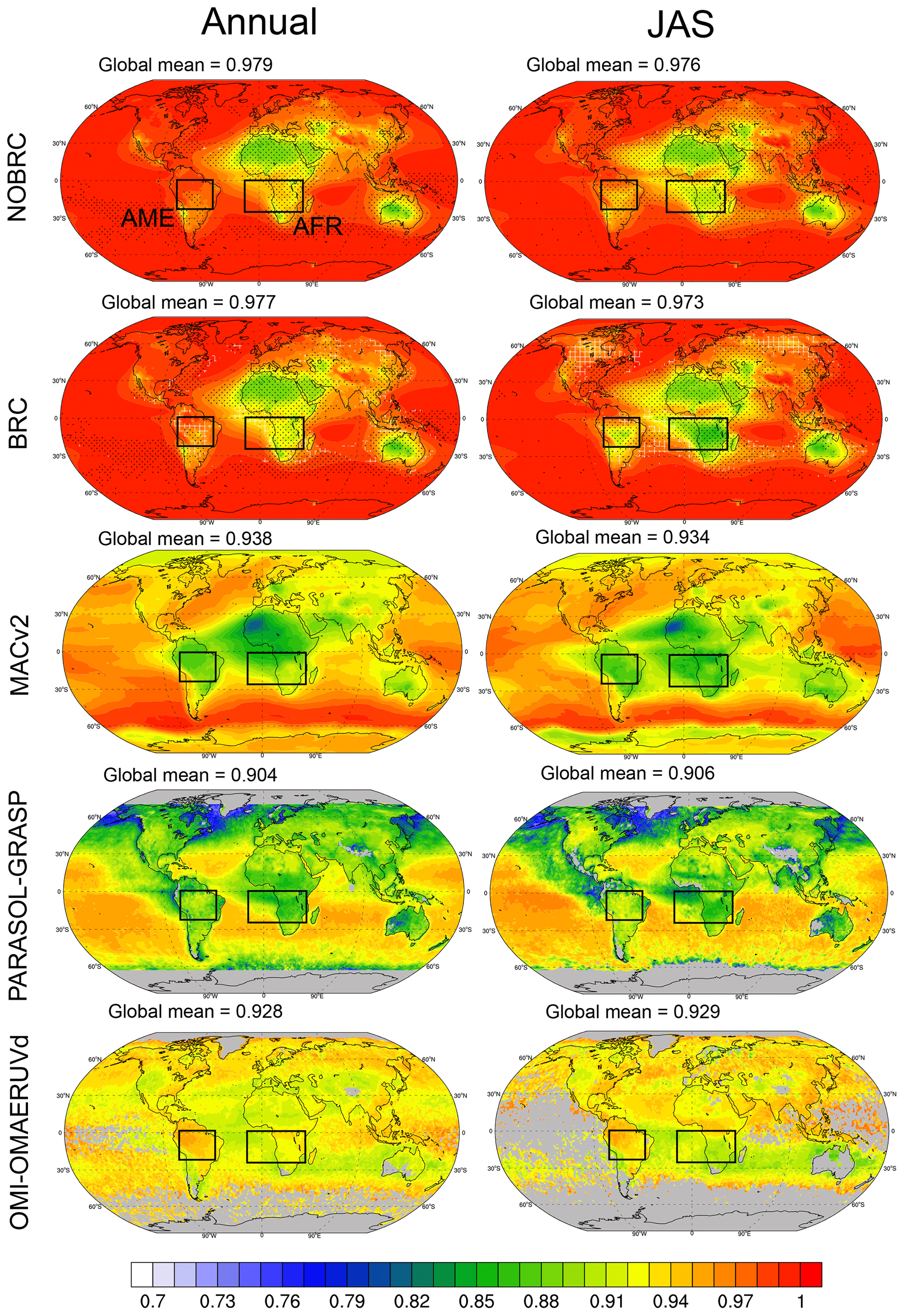
Table 5SSA, AAOD, and AOD annual or JAS averages ±2σ (significance level of 95 %) simulated with (BRC) and without (NOBRC) BrC and provided by reference data sets (PARASOL-GRASP, OMI-OMAERUVd, MACv2, and FMI_SAT; see Table 2 for details) over the AFR and AME regions (see Fig. 1 for details).
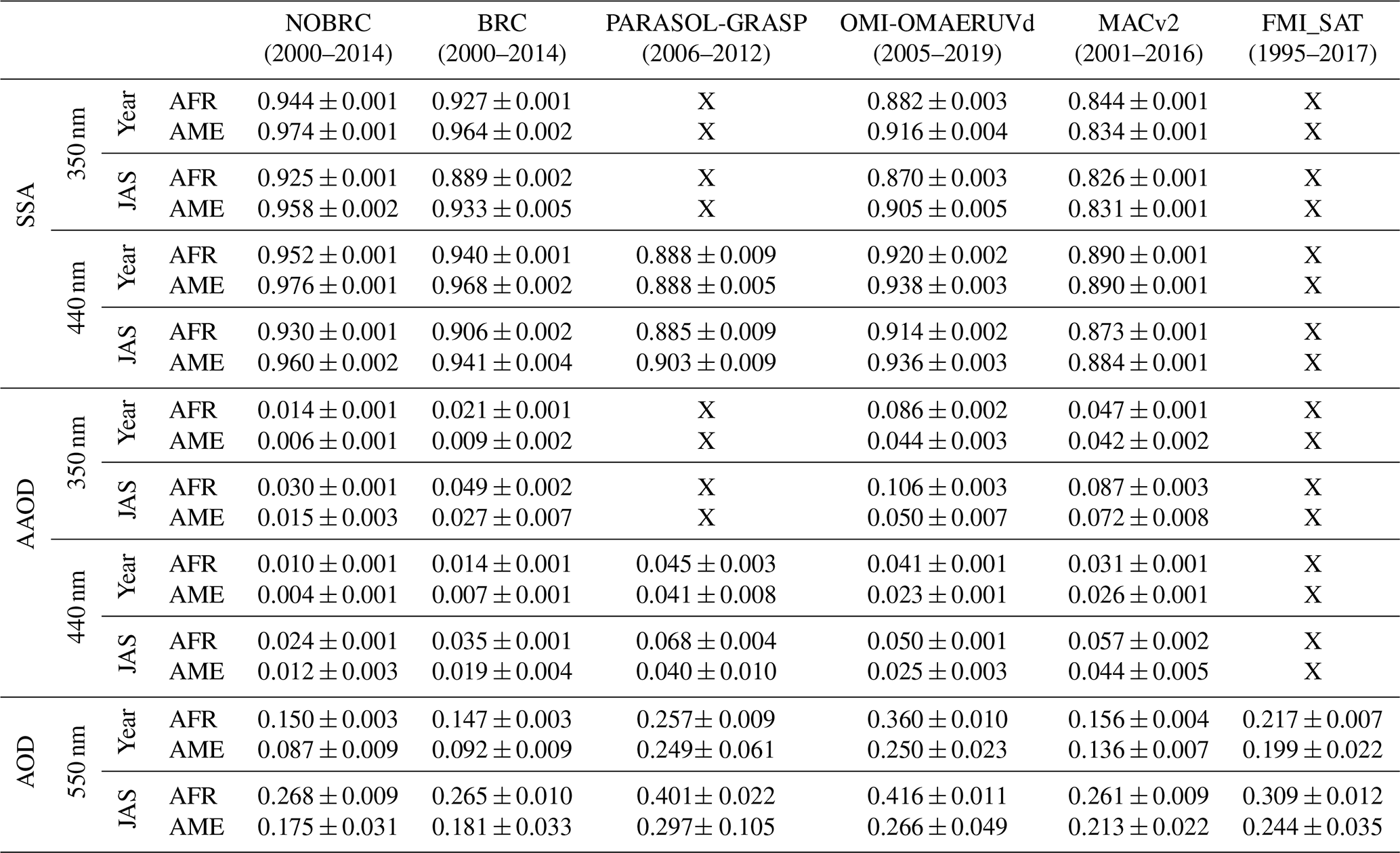
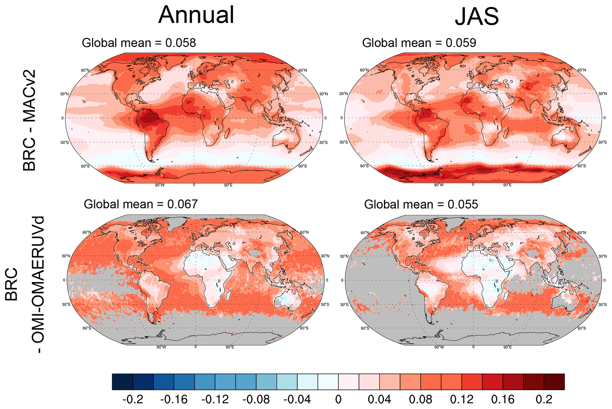
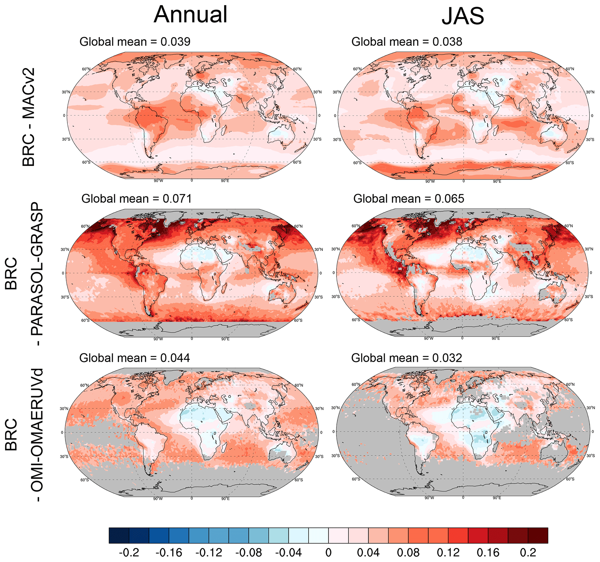
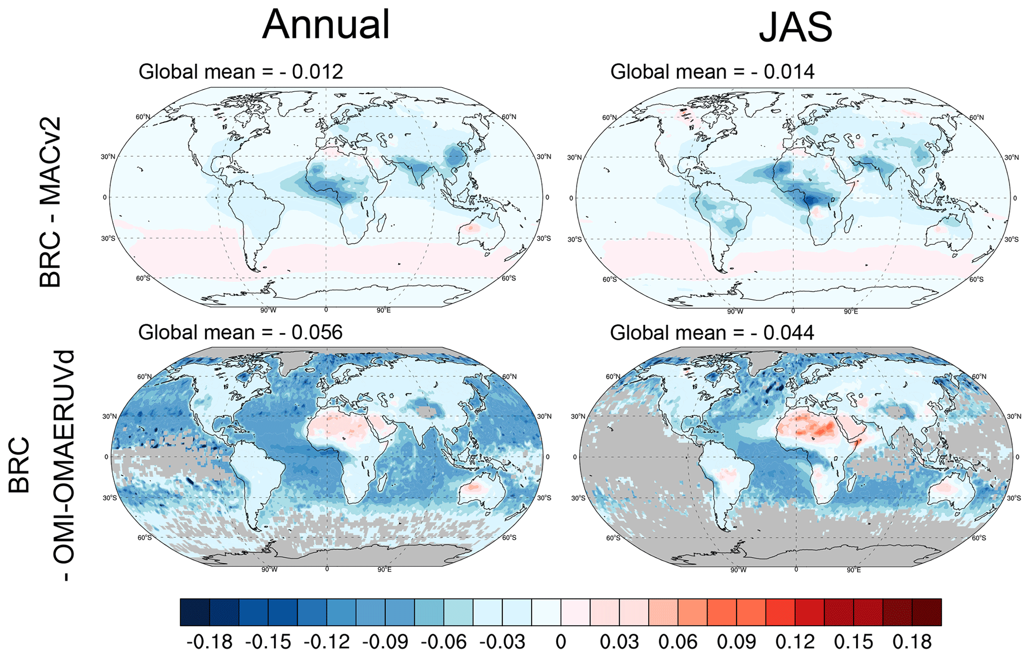
Our second comparison concerns the total AAOD (350 and 440 nm), and we compare the simulated AAOD to the PARASOL-GRASP, OMI-OMAERUVd, and MACv2 products (see Figs. 10 and 11). As for the SSA, we can highlight differences between these three observational data sets. Indeed, at 440 nm, the annual averaged PARASOL-GRASP AAOD is 0.045 ± 0.003 (0.041 ± 0.008) over the AFR (AME) region, while the corresponding values of OMI-OMAERUVd and MACv2 are 0.041 ± 0.001 and 0.031 ± 0.001 (0.023 ± 0.001 and 0.026 ± 0.001). Differences between these data sets can also be observed in other regions such as Australia or China. Compared to these data sets, the NOBRC simulation shows a too low annual AAOD over AFR (0.010 ± 0.001) and AME (0.004 ± 0.001) at 440 nm, while the BRC simulation indicates higher values of 0.014 ± 0.001 (0.007 ± 0.001) over AFR (AME), more consistent with the reference data sets (AAOD differences between BRC and the reference data sets are shown in Fig. A8). Table 5 indicates similar results for the JAS season and for the 350 nm wavelength.
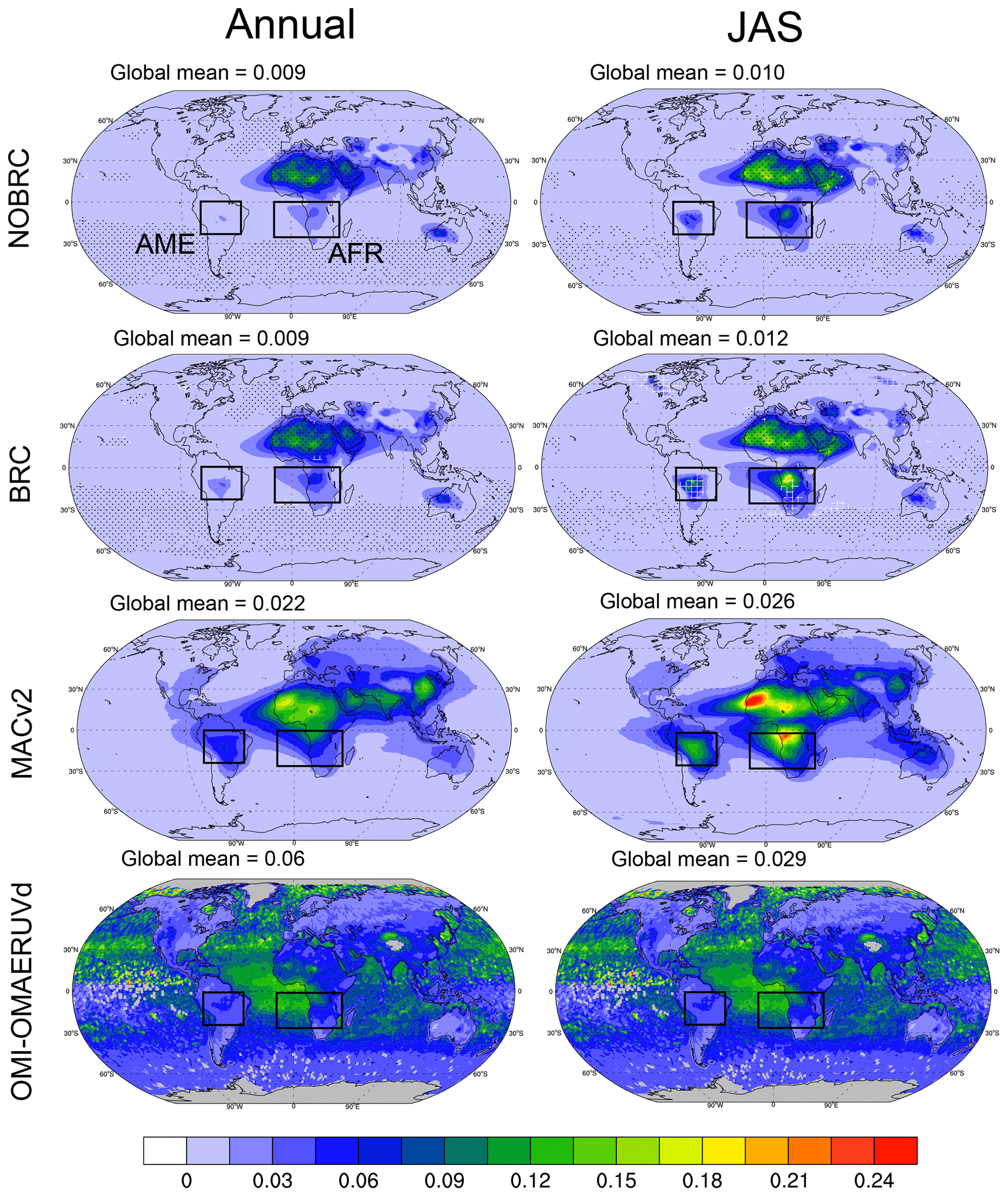
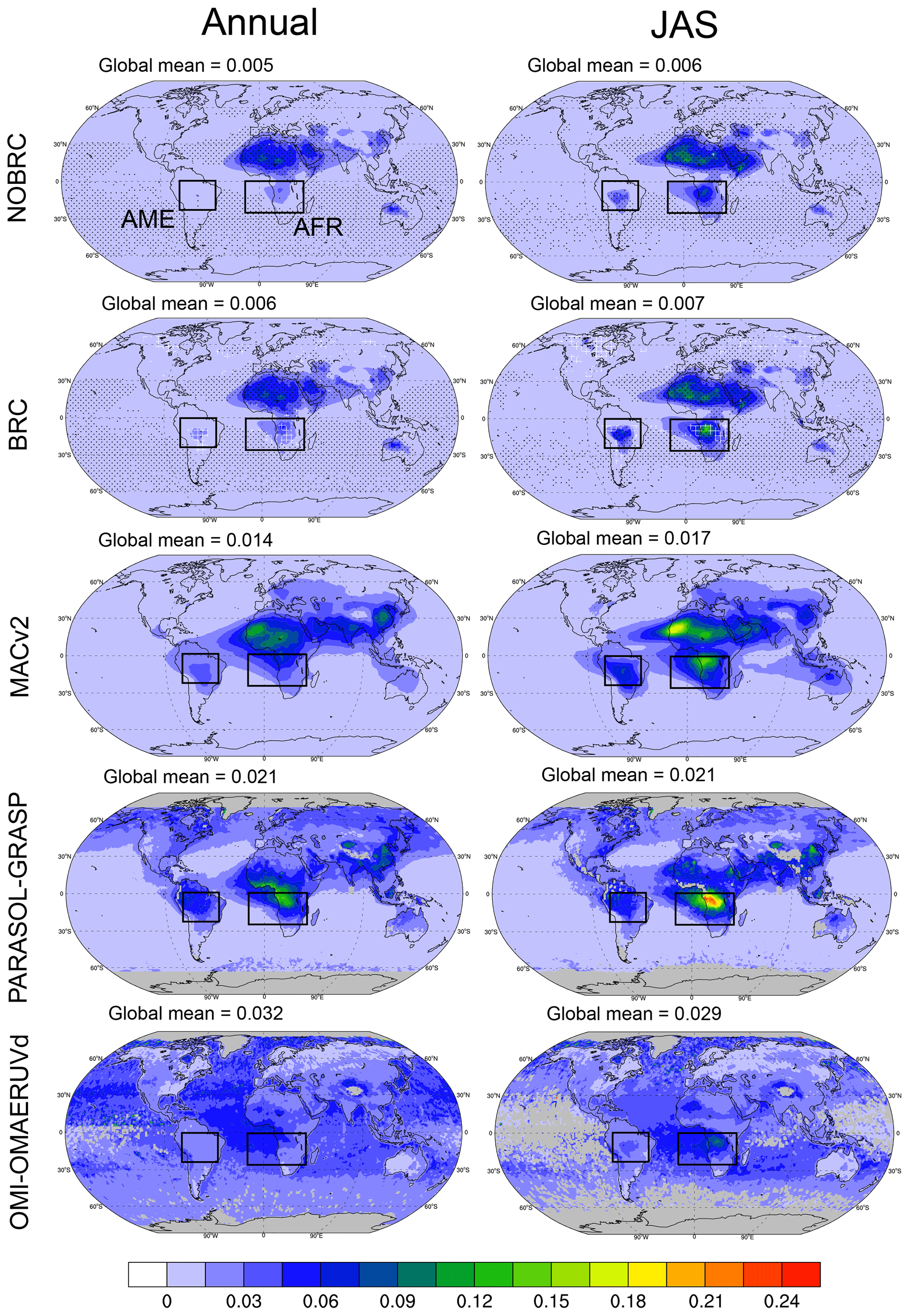
Lastly, Fig. A5 presents the simulated AOD (550 nm) (NOBRC and BRC simulations) and that from the FMI_SAT, MACv2, PARASOL-GRASP, and OMI-OMAERUVd data sets, averaged over the year and over the JAS season. Here too, the reference data sets differ significantly, as illustrated in Fig. A6, which shows the AOD differences with FMI_SAT. Figure A5 shows close annual AODs between NOBRC (0.150 ± 0.003 over AFR and 0.087 ± 0.009 over AME) and BRC (0.147 ± 0.003 over AFR and 0.092 ± 0.009 over AME). The two model runs generally underestimate AOD values compared to the satellite products. For example, NOBRC and BRC present, respectively, a mean annual AOD of 0.150 ± 0.003 and 0.147 ± 0.003 over AFR, while the reference data sets are comprised between 0.156 ± 0.004 and 0.360 ± 0.010.
In summary, the implementation of the BrC parameterization improves the simulated SSA as well as the simulated AAOD, at both 350 and 440 nm and both locally and at a regional scale, more so when the bleaching parameterization is taken into account. Improvements appear in regions and periods where large quantities of biomass burning aerosols are emitted.
4.2 BrC radiative and climatic effects
4.2.1 Brown carbon radiative effect
Figure 12 presents the mean annual and JAS effective radiative forcing from aerosol–radiation interactions (ERFari; see Eq. 4), in clear-sky and all-sky conditions, and from aerosol–cloud interactions (ERFaci, Eq. 5) based on the difference between the BRC and NOBRC simulations. Total ERF, in all-sky conditions, is also presented in this figure. The statistical test applied here is the Wilks test (Wilks, 2006, 2016). All radiative forcing estimates are summarized, for the different regions studied, in Table 6. In clear-sky conditions, the ERFari annual global mean is 0.028 ± 0.013 W m−2, while we compute a stronger value (0.064 ± 0.022 W m−2) during the JAS period. During this season, the highest ERFari is found over regions impacted by BrC, which results in statistically significant warming effects of 0.404 ± 0.100 and 0.358 ± 0.111 W m−2 on average over the AFR region, which has the highest BB emissions (see Fig. 2), and over the AME region, respectively. In clear-sky conditions, the highest values are found over the continents, where they can reach up to 1.5 W m−2. Clear-sky annual (0.029 ± 0.006 W m−2) and JAS (0.062 ± 0.011 W m−2) global averages are similar to all-sky ones. Over the AFR region, Fig. 12 shows statistically significant larger ERFari (0.292 ± 0.034 W m−2 in the annual mean and 0.785 ± 0.110 W m−2 over JAS), notably due to high values over the Atlantic Ocean, up to 1 (4) W m−2 in the annual (JAS) mean, which are due to the presence of stratocumulus and therefore of high albedo. Indeed, in addition to being absorbed in smoke plumes, incoming solar radiation is also reflected by stratocumulus clouds and absorbed again by absorbing biomass burning aerosol (Abel et al., 2005; Zhang et al., 2016). Our results are consistent with those of Brown et al. (2018), who analyze simulations that include or not a bleaching parameterization. Brown et al. (2018) also indicate a positive ERFari in the annual average, especially over the AFR region, with maxima of between 0.8 and 1.7 W m−2 depending on the implementation or not of the BrC bleaching effect. At the global scale, they show an annual mean ERFari between 0.06 (with the BrC bleaching effect) and 0.13 W m−2 (without the BrC bleaching effect). Using the same bleaching parameterization as Brown et al. (2018) in the GEOS-Chem CTM, Wang et al. (2018) calculated an annual global BrC IRF of 0.05 W m−2. Lastly, other studies report annual global BrC direct radiative effects between 0.10 and 0.12 W m−2 (Feng et al., 2013; Wang et al., 2014; Saleh et al., 2015; Jo et al., 2016; Zhang et al., 2020).

Figure 12BrC ERFari (W m−2, clear-sky and all-sky conditions) and ERFaci (W m−2, all-sky conditions) and the sum of both (ERFari + ERFaci, W m−2, all-sky conditions) averaged over the year and over JAS. Hatching indicates regions with a significant effective radiative forcing at the 0.05 level (Wilks test).
Table 6BrC ERFari (W m−2, clear-sky and all-sky conditions), ERFaci (W m−2, all-sky conditions), and ERF (W m−2, all-sky conditions) annual and JAS averages ±2σ (significance level of 95 %) for the BRC simulation at the global scale and over the AME and AFR regions (see Fig. 1 for details).
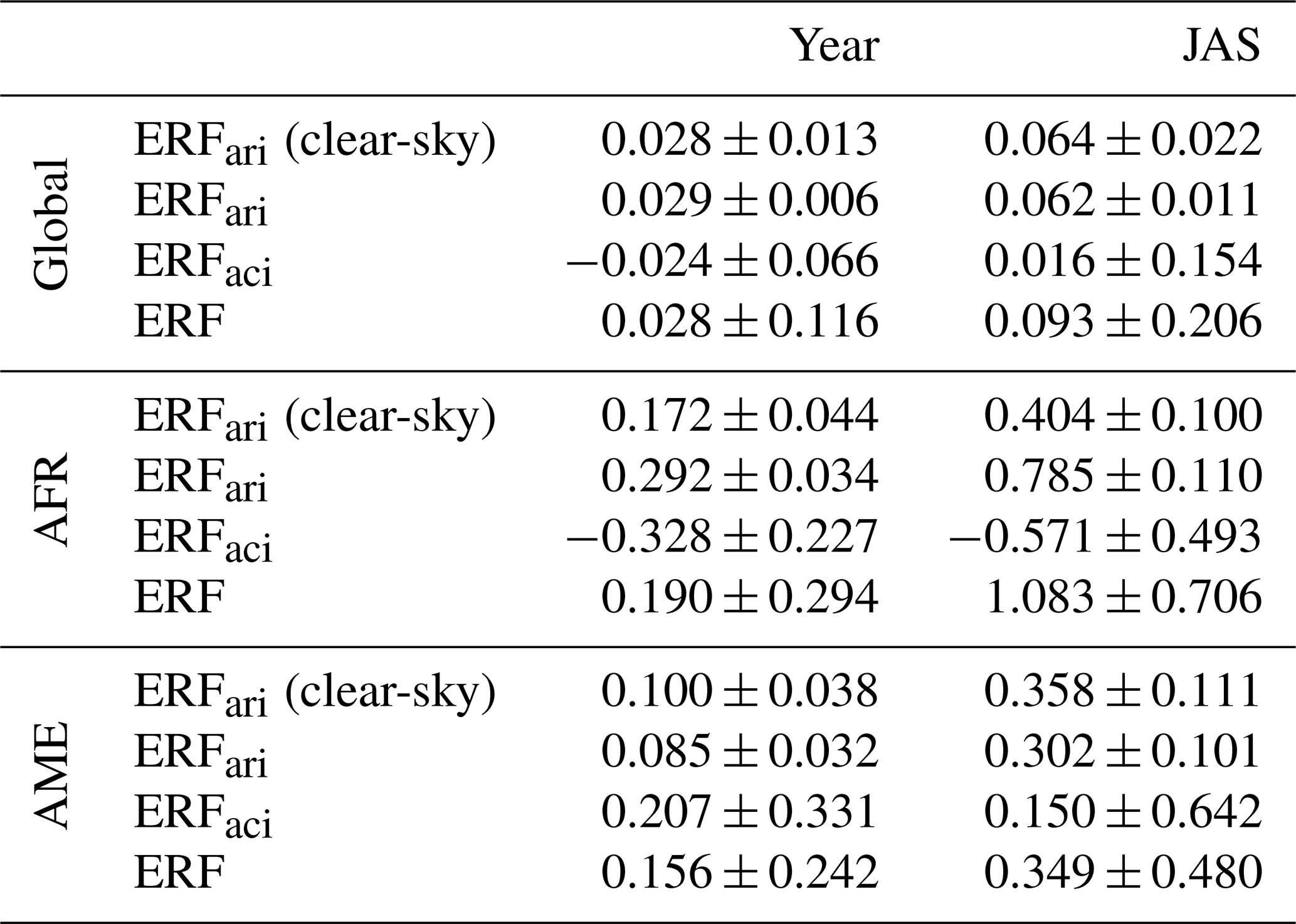
In contrast to ERFari patterns, which are statistically significant and well co-localized with the BB BrC sources, the effective radiative forcing from aerosol–cloud interactions (ERFaci), also shown in Fig. 12, appears less clearly. The mean annual (JAS) global ERFaci is −0.024 ± 0.066 W m−2 (0.016 ± 0.154 W m−2) and therefore too noisy to be meaningful. All ERFaci values, over the different regions studied, are also summarized in Table 6. It is important to remember here that the BrC indirect effect is taken into account in the same way as that of the OA aerosols (hydrophilic bin). In comparison to our results, Brown et al. (2018) found an annual global ERFaci of 0.01 ± 0.04 W m−2 (both with and without a BrC bleaching effect). Over the AFR region, our ERFaci is −0.328 ± 0.227 W m−2 on the annual average (−0.571 ± 0.493 W m−2 over the JAS period), with the most negative values on the ocean side, suggesting that the BrC absorption increases the low cloud formation and lifetime in the model there. These results are consistent with the Sakaeda et al. (2011) and Johnson et al. (2004) studies which show that, over the ocean, the presence of absorbing aerosols above clouds, which increases the potential temperature above the cloud top and therefore creates less favorable conditions for cloud top entrainment, allows for a more persistent low marine cloud cover. Over the AME region, we derive a positive ERFaci of 0.207 ± 0.331 W m−2 on the annual average (0.150 ± 0.642 W m−2 over the JAS period), therefore suggesting a decrease in cloud formation that is also consistent with the Sakaeda et al. (2011) study. Further insight into the BrC effects on clouds in ARPEGE-Climat is presented in Sect. 4.2.2. Finally, in terms of total ERF, we obtain positive annual values of 0.028 ± 0.116 W m−2 at the global scale, of 0.190 ± 0.294 W m−2 over the AFR region, and of 0.156 ± 0.242 W m−2 over the AME region.
4.2.2 Brown carbon effects on temperature and low clouds
Figure 13 and Table 7 present the BrC JAS and annual impacts on low-level (below 640 hPa) cloud fraction and temperature at 700 hPa, calculated as differences between the BRC and NOBRC simulations. For information, no significant BrC impact was found on other meteorological fields often studied such as large-scale/convective precipitation or high-level (above 440 hPa) cloud fraction. On the annual average, Fig. 13 shows no significant effect of BrC on the low-level cloud fraction (−0.008 ± 0.102 %). In their study, Brown et al. (2018) rather show small positive low-level cloud fraction changes (not statistically significant though) between 0.03 and 0.06 ± 0.03 % depending on their BrC parameterization. More regionally and on the seasonal average, Fig. 13 shows an increase in the low-level cloud fraction over the AFR region (0.645 ± 0.342 %) and even more over the OCE region (up to 2 % with an averaged value of 0.723 ± 0.799 %) during JAS. This OCE region (OCEan, 15∘ W–10∘ E/0–25∘ S) is particularly interesting here because it corresponds to the maxima in BrC radiative forcing. It is therefore the region where the rapid responses of the atmosphere will be due to the BrC aerosol plume. The low-level cloud fraction increase over the OCE region during JAS is well correlated with a vertical velocity decrease of about 10 % (−0.004 Pa s−1) at 700 hPa (see Fig. 14). This vertical velocity decrease is consistent with a low-level tropospheric stability increase, leading to a larger low cloud cover in the marine boundary layer. Our results are consistent with those of several studies showing large changes in vertical velocity caused by the absorption of smoke aerosols in the lower troposphere, which could influence the low marine cloud cover. Indeed, a low-level cloud cover increase (decrease) is related to negative (positive) vertical velocity changes (Sakaeda et al., 2011; Wilcox, 2012; Brown et al., 2018; Allen et al., 2019; Deaconu et al., 2019; Mallet et al., 2020). Our study also shows that the augmentation in low-level cloud fraction during JAS over the OCE region is co-located with a negative ERFaci of −0.739 ± 0.934 W m−2 (see Fig. 12). This ERFaci low-level cloud fraction relation is also present over other regions of the globe, such as South America, Europe, North America, India, or China. We computed global spatial correlations of −0.42 (annual average) and −0.47 (JAS average) between these two parameters. The ERFaci low-level cloud fraction relation was also shown in the Brown et al. (2018) study (no value given) over various regions of the world, such as South America, western Australia, the Middle East, or northeastern China.
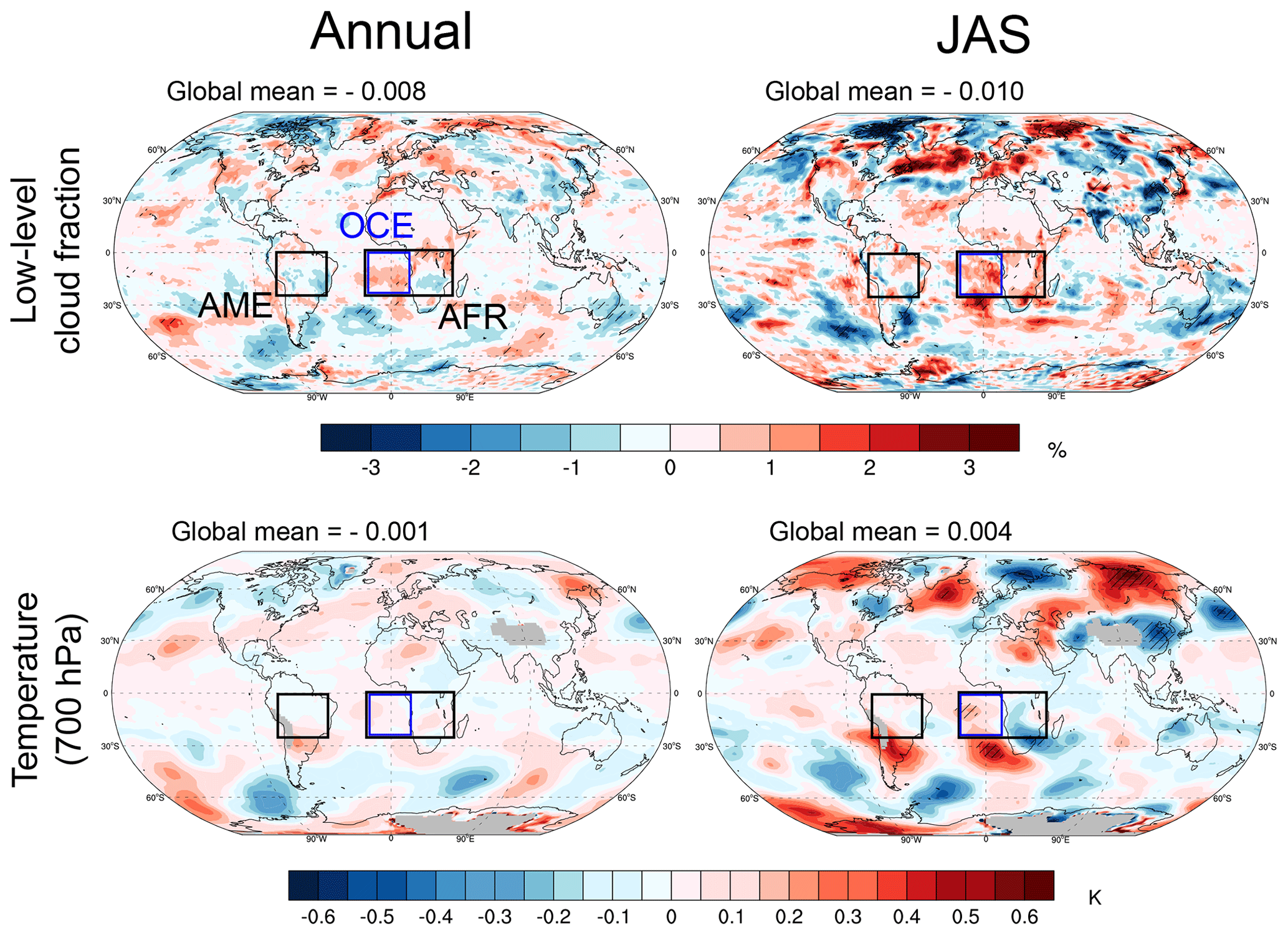
Figure 13Changes between the BRC and NOBRC simulations (BRC minus NOBRC) in low-level (below 640 hPa) cloud fraction (%, relative percentage difference of cloud fraction) and temperature (K, 700 hPa) averaged over the year and over JAS. Hatching indicates regions with a significant effect at the 0.05 level (Wilks test).
Table 7Annual and JAS averages ±2σ (significance level of 95 %) BrC effects (differences between BRC and NOBRC) on low-level cloud fraction (%, relative percentage difference of cloud fraction) and temperature (K, 700 hPa) at the global scale and over the AME, AFR, and OCE regions (see Fig. 1 for details).
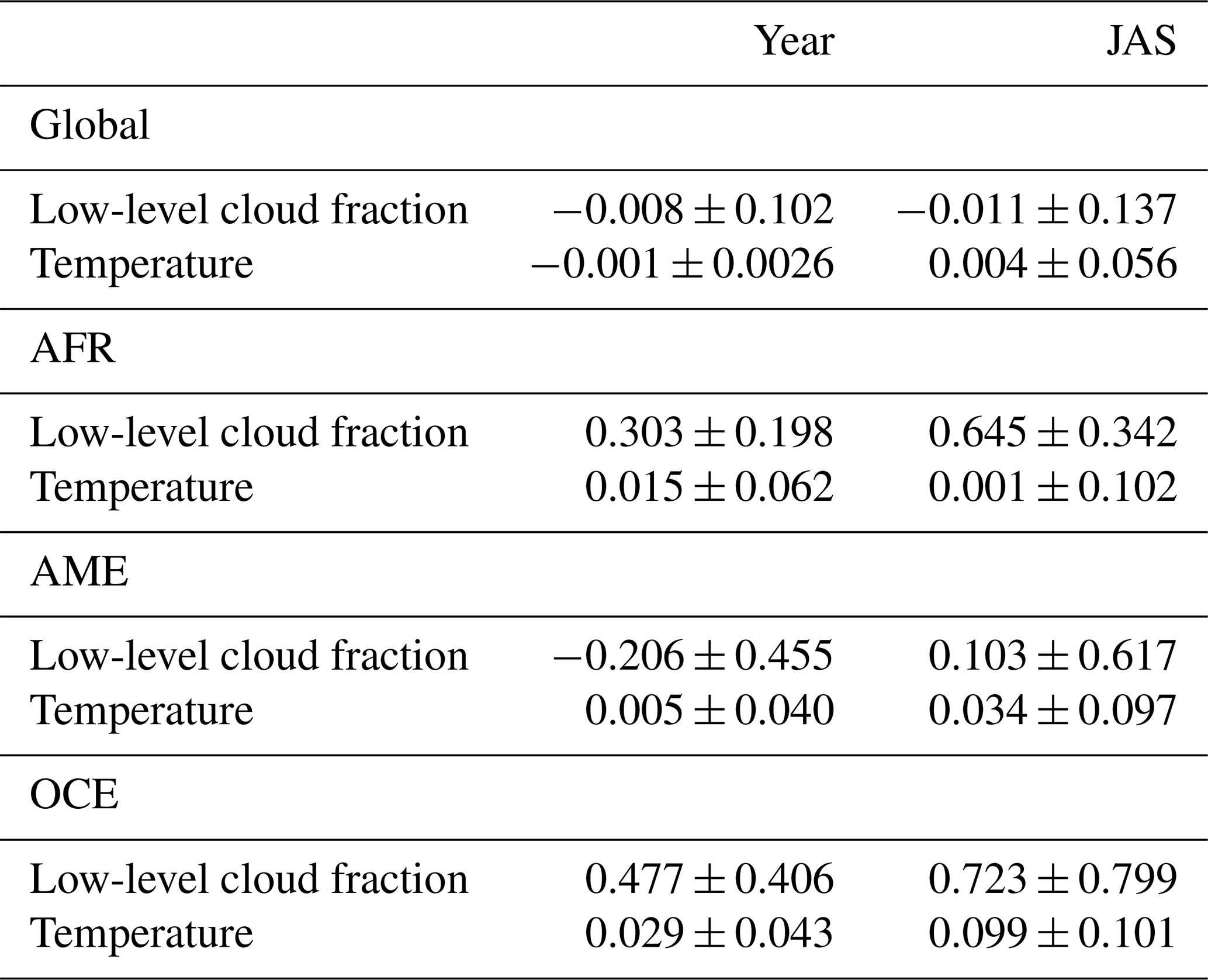
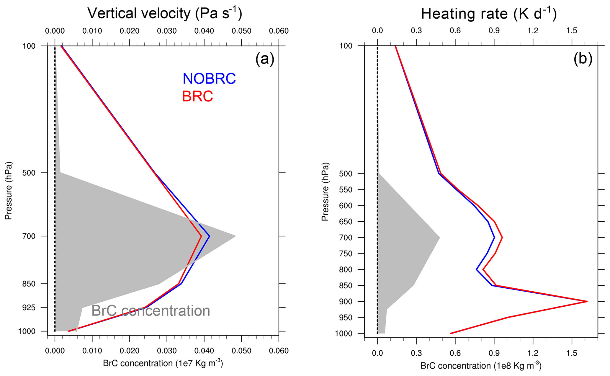
Figure 14JAS mean over the OCE region of vertical velocity (Pa s−1, a) and shortwave heating rate (K d−1, b). BrC concentrations have been added in both figures (note the different x axes).
Lastly, temperature changes at 700 hPa (altitude with the most smoke aerosol transport, Das et al., 2017) due to the BrC addition to the model are shown in Fig. 13. Small and no statistically significant effects can be seen on annual averages (−0.001 ± 0.026 ∘C global mean). Over JAS, Fig. 13 shows statistically significant larger changes, up to +0.6 ∘C in northern Russia and up to 0.5 ∘C in the south of the OCE region. Conversely, statistically significant temperature decreases, up to −0.5 ∘C, can be observed, as for example in eastern China. Over these regions, the temperature shifts would rather be related to climate feedbacks, teleconnections, or even changes in atmospheric dynamics but not directly to BrC aerosol plumes. Over the OCE region, directly impacted by a BrC aerosol plume, the temperature increase (0.099 ± 0.101 ∘C) is mostly caused by smoke aerosol solar absorption associated with a (solar) heating rate increase of about 0.1 K d−1 (11 %; see Fig. 14). Above 800 hPa, this heating rate increase is largely due to the absorption of BrC particles, while between 800 and 850 hPa, the heating rate increase is also due in part to the low-level cloud fraction increase described previously. It still remains important to remind the reader here that the ARPEGE-Climat global atmospheric model is run in an AMIP-type mode, and therefore coupled ocean–atmosphere simulations would be relevant to consolidate, or not, our results.
Organic aerosols have long been considered to be only scattering aerosols, but recent studies have shown that a part of these aerosols, called brown carbon particles, can absorb solar radiation. In parallel, several multi-model studies have led to the conclusion that models underestimate the AAOD: Shindell et al. (2013) showed an AAOD underestimation by the ACCMIP models compared to the AERONET stations, especially over South America and Southern Hemisphere Africa, while very recently, Mallet et al. (2021) demonstrated that the majority of CMIP6 global climate models underestimate the absorption of biomass burning aerosols over the southeastern Atlantic. With emerging evidence of the importance of BrC, especially for solar absorption at UV and short visible wavelengths, all this has led to the inclusion of BrC in chemical transport models and, more recently, in some global climate models.
In this work, we have implemented a BrC parameterization, derived from Saleh et al. (2014), in the TACTIC aerosol scheme of ARPEGE-Climat, the atmospheric component of the CNRM global climate model. We have conducted a BrC radiative and climatic effect study thanks to several simulations over the period of 2000–2014. The implementation of a BrC parameterization in climate models can be done in several ways. The method we adopted, which allows for a good representation of the spatial and temporal variability of the BrC absorption, consists in parameterizing the BrC imaginary refractive index according to the BC-to-OA ratio in emissions (Saleh et al., 2015; Brown et al., 2018; Wang et al., 2018). As recent studies have shown similar results using, or not, a constant BC-to-OA ratio (Brown et al., 2018; Wang et al., 2018), we have therefore chosen to use a constant (0.08) BC-to-OA ratio. The effect of bleaching has also been included.
The implementation of BrC particles in TACTIC has allowed for a significant improvement of several total aerosol optical properties, such as the total aerosol SSA and AAOD, at both the local and regional scales. This betterment occurred particularly at 350 and 440 nm in regions with high biomass burning emissions (AFR and AME) which are the main sources of BrC. However, at certain African and South American AERONET sites, climatological AAOD are still slightly underestimated by our model. One hypothesis to explain this bias may be related to the spatial and temporal representativeness of the AERONET data. It is also likely that part of the differences between the model and the reference data sets could come from the emission inventories used in this study. However, we have outlined a strong disparity between the different reference data sets used in this work and ground-based and satellite data (PARASOL-GRASP, OMI-OMAERUVd, MACv2, FMI_SAT) on all the studied parameters, and this highlights the need for further work to provide modelers with solid reference data sets.
We computed annual and JAS BrC ERFs (ERFari, ERFaci, and total ERF) at both the global and regional scales. In all-sky conditions, the annual global BrC ERFari is 0.029 ± 0.006 W m−2, while the BrC ERFaci is −0.024 ± 0.066 W m−2. At the regional scale, over regions impacted by BrC, our BrC ERFari warming effect goes up to 0.085 ± 0.032 W m−2 (AME region) and to 0.292 ± 0.034 W m−2 (statistically significant, AFR region). While ERFari patterns are statistically significant and well co-localized with BrC sources, ERFaci patterns are more patchy with a lot of regional differences, ranging from −2.5 to 2.5 W m−2. We derive from our study a small annual global BrC ERF of 0.028 ± 0.116 W m−2, with maximum values over the AFR region (0.190 ± 0.294 W m−2). Our ERF results compare relatively well to those of Brown et al. (2018) when these authors consider a BrC bleaching parameterization that reduces by half their BrC radiative forcing. While we have some confidence in comparing our study to that of Brown et al. (2018), which follows to some extent the protocol we use (the Ghan, 2013, formulation, AMIP-type simulations with and without BrC), it does not seem appropriate to compare our results to others in the literature (see our introduction) that use different methodologies or present different radiative forcing concepts (e.g., IRF). We believe that our results, which follow the CMIP6 AerChemMIP (Collins et al., 2017) and RFMIP (Pincus et al., 2016) recommendations, are solid.
Taking into account the BrC effect, and therefore the absorption increase in biomass burning plumes, contributes moderately to a low-level cloud fraction change. Indeed, a slight low-level cloud fraction increase (0.723 ± 0.799 %) was simulated over the OCE region during JAS. This low-level cloud fraction increase is due to a low-level tropospheric stability increase, caused at least in part by a 700 hPa vertical velocity decrease of about 10 %. Mallet et al. (2021) have shown that the frequent underestimation of biomass burning aerosol absorption by climate models over the southeastern Atlantic could lead to a misrepresentation of the low-level cloud response. Their study highlights the importance for climate models to properly represent the biomass burning aerosol absorption and consequently the need to consider BrC aerosols. Finally, in terms of climatic impacts, we simulated a moderate 700 hPa temperature increase (0.099 ± 0.101 ∘C) over the OCE region during JAS. This temperature augmentation is caused not only by a heating rate increase of about 11 %, but also by the low-level cloud fraction increase over this region.
The results presented in this study highlight the importance of taking the BrC aerosols into account in climate models. Nevertheless, several hypotheses would have to be tested to further evaluate our model sensitivity and possibly improve the model in terms of both radiative and climatic impacts. These hypotheses include the BrC lifetime or the use of different BC-to-OA ratios for BB and BF emissions that would allow for the differentiation of the BrC optical properties according to the source of emissions. We have to note however that further studies are needed, in addition to those already published (e.g., Zhong and Jang, 2011; Lee et al., 2014; Forrister et al., 2015; Zhao et al., 2015; Wang et al., 2016; Vakkari et al., 2018), to improve the knowledge about BrC, for instance, on the BrC aging processes (e.g., formation of secondary BrC, lifetime, evolution of the absorption). Finally, fully coupled atmosphere–ocean climate model simulations would be relevant to allow for the BrC absorption to affect air–sea interactions.
Table A1Aerosol optical properties, namely, extinction cross section (Ext in m2 g−1), single-scattering albedo (SSA), and asymmetry parameter (g) used in the present version of TACTIC at 350 and 550 nm. Values are given for relative humidities of 0 % and 80 %. Bin diameter limits (µm) are given in parentheses for SS and DD aerosols.

Table A2References of the refractive indices associated with the aerosol types in ARPEGE-Climat. The organic aerosol type is a combination of three OPAC types similar to a continental mixture, as described in Hess et al. (1998).
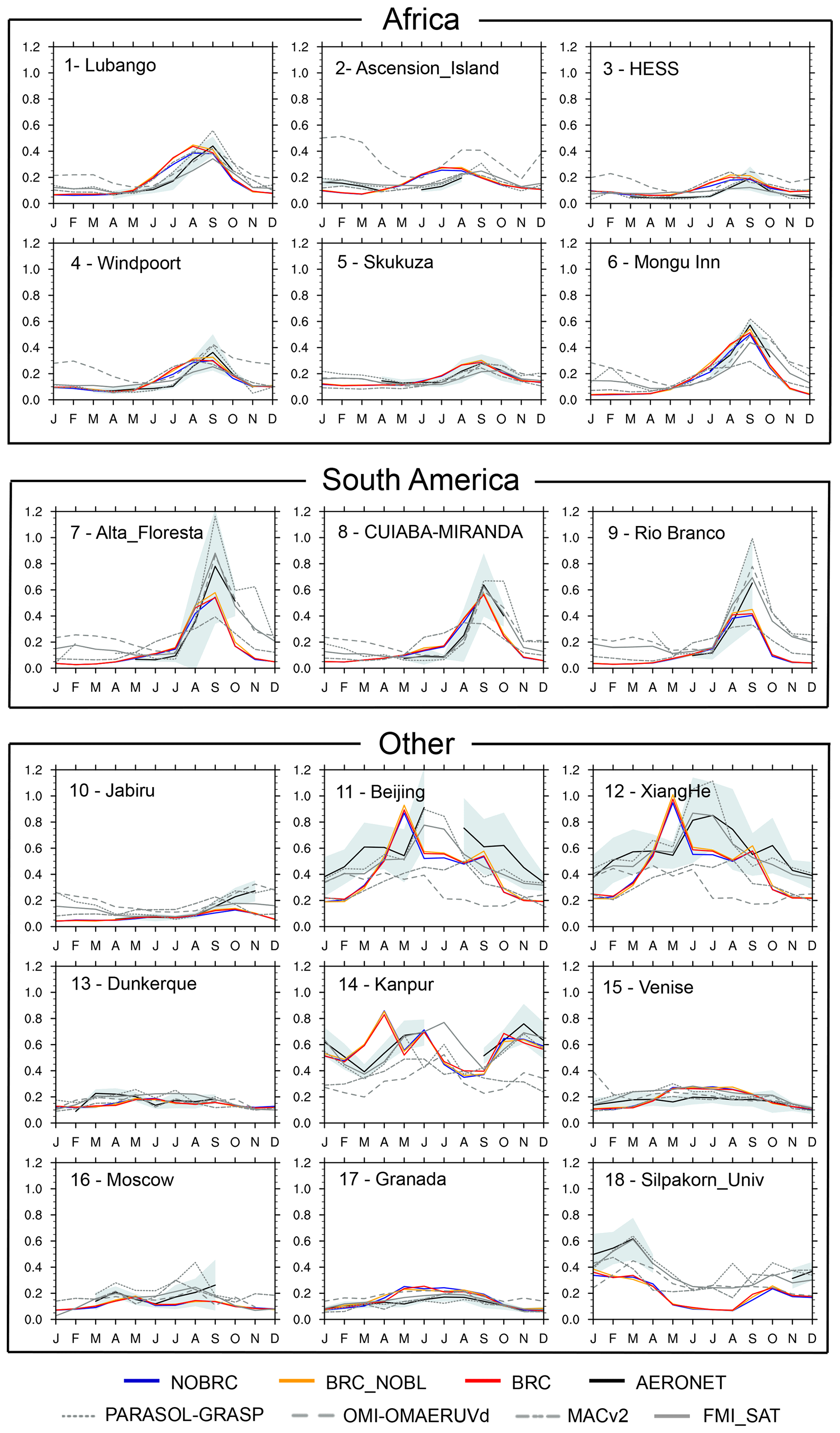
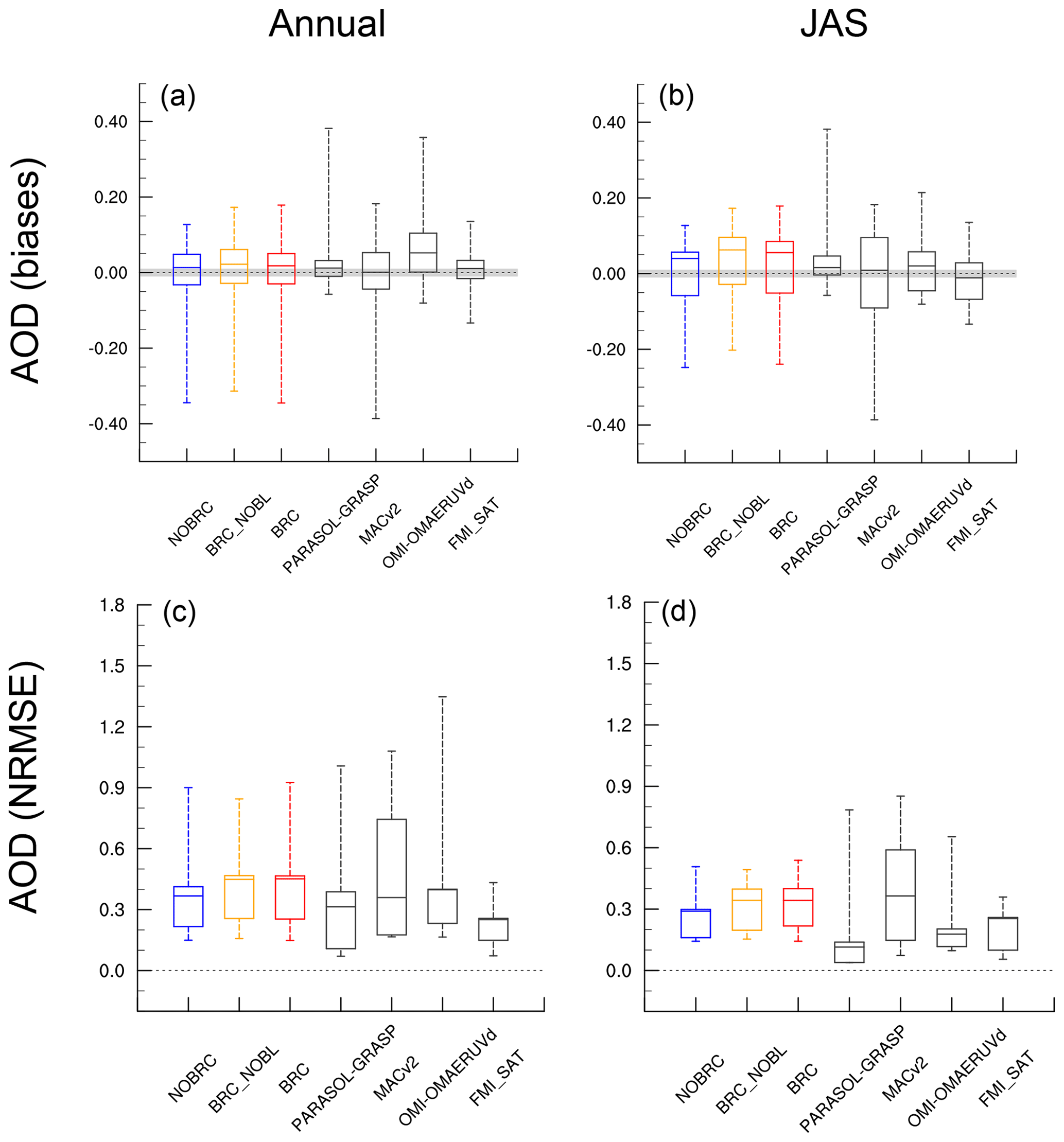
Figure A2Boxplots of AOD (550 nm) various biases (a, b) and normalized root mean square error (NRMSE, c, d) compared to the AERONET observations, over the year (a, c) and over JAS (b, d). Simulations: NOBRC, BRC_NOBL, and BRC (see Table 3 for details) and reference data sets (PARASOL-GRASP, OMI-OMAERUVd, MACv2, FMI_SAT; see Table 2 for details). Uncertainty of the AERONET observations appears shaded.


This study relies entirely on publicly available data. Codes of the various components of the ARPEGE-Climat model are available as follows: the SURFEX code is accessible using a CECILL-C license (http://www.cecill.info/licences/Licence_CeCILL-C_V1-en.txt, last access: 14 September 2022) at http://www.umr-cnrm.fr/surfex (last access: 14 September 2022, CNRM, 2022). OASIS3-MCT is available at https://oasis.cerfacs.fr/en/ (last access: 14 September 2022, CERFACS, 2022), XIOS at https://forge.ipsl.jussieu.fr/ioserver (last access: 14 September 2022, XIOS, 2022), and the rest of the ARPEGE-Climat code upon request to the authors. The outputs of the different simulations presented here are available upon request from the authors (thomas.druge@meteo.fr). PARASOL-GRASP data are publicly available on the official GRASP algorithm website at https://www.grasp-open.com/products (last access: 23 February 2022, GRASP, 2022). The OMI-OMAERUVd product can be obtained from the NASA Earth data portal at https://doi.org/10.5067/Aura/OMI/DATA3003 (Torres, 2008). The MACv2 product is available at ftp://ftp-projects.mpimet.mpg.de/aerocom/climatology/MACv2_2018/ (last access: 23 February 2022, Max Planck institute Aerosol climatology, 2022). FMI_SAT data are available at http://nsdc.fmi.fi/data/data_aod (last access: 23 February 2022, Finnish Meteorological Institute, 2022). Lastly, AERONET data are available at https://aeronet.gsfc.nasa.gov/ (last access: 23 February 2022, Aerosol Robotic Network, 2022).
TD wrote the paper with contributions from all co-authors. TD, PN, MMa, MMi, SR, and OD designed the experimental methodology and participated in the analyses. TD, PN, MMa, MMi, and SR contributed to the model development. OD specifically contributed to the satellite portion of this work.
The contact author has declared that none of the authors has any competing interests.
Publisher’s note: Copernicus Publications remains neutral with regard to jurisdictional claims in published maps and institutional affiliations.
This work has received funding from the EU-funded Copernicus Atmospheric Monitoring Services 43 “Development of global aerosol aspects” (CAMS_43) project as well as from the EU Horizon 2020 Research and Innovation program under grant agreement no. 101003536 (ESM2025 – Earth System Models for the Future). We are grateful to the principal investigators of the AERONET network and its staff for establishing and maintaining the different sites used in this investigation. All providers of satellite data are thanked for making available their aerosol data sets. We were also supported by the entire team in charge of the CNRM climate models. Supercomputing time was provided by the Météo-France/DSI supercomputing center.
This research has been supported by the EU-funded Copernicus Atmospheric Monitoring Services 43 “Development of global aerosol aspects” (CAMS_43) project as well as by the EU Horizon 2020 Research and Innovation program under grant agreement no. 101003536 (ESM2025 – Earth System Models for the Future).
This paper was edited by Kostas Tsigaridis and reviewed by two anonymous referees.
Abel, S. J., Highwood, E. J., Haywood, J. M., and Stringer, M. A.: The direct radiative effect of biomass burning aerosols over southern Africa, Atmos. Chem. Phys., 5, 1999–2018, https://doi.org/10.5194/acp-5-1999-2005, 2005. a
Ackerman, T. P. and Toon, O. B.: Absorption of visible radiation in atmosphere containing mixtures of absorbing and nonabsorbing particles, Appl. Optics, 20, 3661–3668, https://doi.org/10.1364/AO.20.003661, 1981. a
Aerosol Robotic Network: AERONET, Goddard Space flight center [data set], https://aeronet.gsfc.nasa.gov/, last access: 23 February 2022. a
Akagi, S. K., Yokelson, R. J., Wiedinmyer, C., Alvarado, M. J., Reid, J. S., Karl, T., Crounse, J. D., and Wennberg, P. O.: Emission factors for open and domestic biomass burning for use in atmospheric models, Atmos. Chem. Phys., 11, 4039–4072, https://doi.org/10.5194/acp-11-4039-2011, 2011. a
Alexander, D. T., Crozier, P. A., and Anderson, J. R.: Brown carbon spheres in East Asian outflow and their optical properties, Science, 321, 833–836, https://doi.org/10.1126/science.1155296, 2008. a
Allen, R. J., Amiri-Farahani, A., Lamarque, J.-F., Smith, C., Shindell, D., Hassan, T., and Chung, C. E.: Observationally constrained aerosol–cloud semi-direct effects, npj Climate and Atmospheric Science, 2, 1–12, https://doi.org/10.1038/s41612-019-0073-9, 2019. a
Andreae, M. O.: Emission of trace gases and aerosols from biomass burning – an updated assessment, Atmos. Chem. Phys., 19, 8523–8546, https://doi.org/10.5194/acp-19-8523-2019, 2019. a
Andreae, M. O. and Gelencsér, A.: Black carbon or brown carbon? The nature of light-absorbing carbonaceous aerosols, Atmos. Chem. Phys., 6, 3131–3148, https://doi.org/10.5194/acp-6-3131-2006, 2006. a
Arola, A., Schuster, G., Myhre, G., Kazadzis, S., Dey, S., and Tripathi, S. N.: Inferring absorbing organic carbon content from AERONET data, Atmos. Chem. Phys., 11, 215–225, https://doi.org/10.5194/acp-11-215-2011, 2011. a, b
Bahadur, R., Praveen, P. S., Xu, Y., and Ramanathan, V.: Solar absorption by elemental and brown carbon determined from spectral observations, P. Natl. Acad. Sci. USA, 109, 17366–17371, https://doi.org/10.1073/pnas.1205910109, 2012. a, b, c
Berglen, T. F., Berntsen, T. K., Isaksen, I. S. A., and Sundet, J. K.: A global model of the coupled sulfur/oxidant chemistry in the troposphere: The sulfur cycle, J. Geophys. Res.-Atmos., 109, D19310, https://doi.org/10.1029/2003JD003948, 2004. a
Bermejo, R. and Conde, J.: A Conservative Quasi-Monotone Semi-Lagrangian Scheme, Mon. Weather Rev., 130, 423–430, https://doi.org/10.1175/1520-0493(2002)130<0423:ACQMSL>2.0.CO;2, 2002. a
Bond, T. C., Doherty, S. J., Fahey, D. W., Forster, P. M., Berntsen, T., DeAngelo, B. J., Flanner, M. G., Ghan, S., Kärcher, B., Koch, D., Kinne, S., Kondo, Y., Quinn, P. K., Sarofim, M. C., Schultz, M. G., Schulz, M., Venkataraman, C., Zhang, H., Zhang, S., Bellouin, N., Guttikunda, S. K., Hopke, P. K., Jacobson, M. Z., Kaiser, J. W., Klimont, Z., Lohmann, U., Schwarz, J. P., Shindell, D., Storelvmo, T., Warren, S. G., and Zender, C. S.: Bounding the role of black carbon in the climate system: A scientific assessment, J. Geophys. Res.-Atmos., 118, 5380–5552, https://doi.org/10.1002/jgrd.50171, 2013. a
Bourgeois, Q. and Bey, I.: Pollution transport efficiency toward the Arctic: Sensitivity to aerosol scavenging and source regions, J. Geophys. Res., 116, D08213, https://doi.org/10.1029/2010JD015096, 2011. a, b
Brown, H., Liu, X., Feng, Y., Jiang, Y., Wu, M., Lu, Z., Wu, C., Murphy, S., and Pokhrel, R.: Radiative effect and climate impacts of brown carbon with the Community Atmosphere Model (CAM5), Atmos. Chem. Phys., 18, 17745–17768, https://doi.org/10.5194/acp-18-17745-2018, 2018. a, b, c, d, e, f, g, h, i, j, k, l, m, n, o, p, q, r, s
Burkholder, J., Sander, S., Abbatt, J., Barker, J., Huie, R., Kolb, C., Kurylo, M., Orkin, V., Wilmouth, D., and Wine, P.: Chemical Kinetics and Photochemical Data for Use in Atmospheric Studies, Evaluation Number 18, Tech. rep., JPL Publication 15-10, Jet Propulsion Laboratory, Pasadena, USA, https://doi.org/10.13140/RG.2.1.2504.2806, 2015. a
CERFACS: The OASIS Coupler, CERFACS [code], https://oasis.cerfacs.fr/en/, last access: 14 September 2022. a
Chakrabarty, R. K., Moosmüller, H., Chen, L.-W. A., Lewis, K., Arnott, W. P., Mazzoleni, C., Dubey, M. K., Wold, C. E., Hao, W. M., and Kreidenweis, S. M.: Brown carbon in tar balls from smoldering biomass combustion, Atmos. Chem. Phys., 10, 6363–6370, https://doi.org/10.5194/acp-10-6363-2010, 2010. a
Chen, C., Dubovik, O., Fuertes, D., Litvinov, P., Lapyonok, T., Lopatin, A., Ducos, F., Derimian, Y., Herman, M., Tanré, D., Remer, L. A., Lyapustin, A., Sayer, A. M., Levy, R. C., Hsu, N. C., Descloitres, J., Li, L., Torres, B., Karol, Y., Herrera, M., Herreras, M., Aspetsberger, M., Wanzenboeck, M., Bindreiter, L., Marth, D., Hangler, A., and Federspiel, C.: Validation of GRASP algorithm product from POLDER/PARASOL data and assessment of multi-angular polarimetry potential for aerosol monitoring, Earth Syst. Sci. Data, 12, 3573–3620, https://doi.org/10.5194/essd-12-3573-2020, 2020. a, b, c
Chen, Y. and Bond, T. C.: Light absorption by organic carbon from wood combustion, Atmos. Chem. Phys., 10, 1773–1787, https://doi.org/10.5194/acp-10-1773-2010, 2010. a, b
Chung, C. E., Kim, S.-W., Lee, M., Yoon, S.-C., and Lee, S.: Carbonaceous aerosol AAE inferred from in-situ aerosol measurements at the Gosan ABC super site, and the implications for brown carbon aerosol, Atmos. Chem. Phys., 12, 6173–6184, https://doi.org/10.5194/acp-12-6173-2012, 2012. a
CNRM: SURFEX, Centre National de Recherches Météorologiques [code], http://www.umr-cnrm.fr/surfex, last access: 14 September 2022. a
Collins, W. J., Lamarque, J.-F., Schulz, M., Boucher, O., Eyring, V., Hegglin, M. I., Maycock, A., Myhre, G., Prather, M., Shindell, D., and Smith, S. J.: AerChemMIP: quantifying the effects of chemistry and aerosols in CMIP6, Geosci. Model Dev., 10, 585–607, https://doi.org/10.5194/gmd-10-585-2017, 2017. a
Das, S., Harshvardhan, H., Bian, H., Chin, M., Curci, G., Protonotariou, A. P., Mielonen, T., Zhang, K., Wang, H., and Liu, X.: Biomass burning aerosol transport and vertical distribution over the South African-Atlantic region, J. Geophys. Res.-Atmos., 122, 6391–6415, https://doi.org/10.1002/2016JD026421, 2017. a
Deaconu, L. T., Ferlay, N., Waquet, F., Peers, F., Thieuleux, F., and Goloub, P.: Satellite inference of water vapour and above-cloud aerosol combined effect on radiative budget and cloud-top processes in the southeastern Atlantic Ocean, Atmos. Chem. Phys., 19, 11613–11634, https://doi.org/10.5194/acp-19-11613-2019, 2019. a
de Bruine, M., Krol, M., van Noije, T., Le Sager, P., and Röckmann, T.: The impact of precipitation evaporation on the atmospheric aerosol distribution in EC-Earth v3.2.0, Geosci. Model Dev., 11, 1443–1465, https://doi.org/10.5194/gmd-11-1443-2018, 2018. a
Decharme, B., Delire, C., Minvielle, M., Colin, J., Vergnes, J.-P., Alias, A., Saint-Martin, D., Séférian, R., Sénési, S., and Voldoire, A.: Recent Changes in the ISBA-CTRIP Land Surface System for Use in the CNRM-CM6 Climate Model and in Global Off-Line Hydrological Applications, J. Adv. Model. Earth Syst., 11, 1207–1252, https://doi.org/10.1029/2018MS001545, 2019. a, b
Dentener, F., Kinne, S., Bond, T., Boucher, O., Cofala, J., Generoso, S., Ginoux, P., Gong, S., Hoelzemann, J. J., Ito, A., Marelli, L., Penner, J. E., Putaud, J.-P., Textor, C., Schulz, M., van der Werf, G. R., and Wilson, J.: Emissions of primary aerosol and precursor gases in the years 2000 and 1750 prescribed data-sets for AeroCom, Atmos. Chem. Phys., 6, 4321–4344, https://doi.org/10.5194/acp-6-4321-2006, 2006. a
Desyaterik, Y., Sun, Y., Shen, X., Lee, T., Wang, X., Wang, T., and Collett, J. L.: Speciation of “brown” carbon in cloud water impacted by agricultural biomass burning in eastern China, J. Geophys. Res.-Atmos., 118, 7389–7399, https://doi.org/10.1002/jgrd.50561, 2013. a
Di Biagio, C., Formenti, P., Balkanski, Y., Caponi, L., Cazaunau, M., Pangui, E., Journet, E., Nowak, S., Andreae, M. O., Kandler, K., Saeed, T., Piketh, S., Seibert, D., Williams, E., and Doussin, J.-F.: Complex refractive indices and single-scattering albedo of global dust aerosols in the shortwave spectrum and relationship to size and iron content, Atmos. Chem. Phys., 19, 15503–15531, https://doi.org/10.5194/acp-19-15503-2019, 2019. a
Drakousis, P., Korras-Carraca, M.-B., Jethva, H., Torres, O., and Hatzianastassiou, N.: Global OMI Aerosol Single Scattering Albedo evaluation using ground-based AERONET, EGU General Assembly 2020, Online, 4–8 May 2020, EGU2020-18209, https://doi.org/10.5194/egusphere-egu2020-18209, 2020. a
Drugé, T., Nabat, P., Mallet, M., and Somot, S.: Model simulation of ammonium and nitrate aerosols distribution in the Euro-Mediterranean region and their radiative and climatic effects over 1979–2016, Atmos. Chem. Phys., 19, 3707–3731, https://doi.org/10.5194/acp-19-3707-2019, 2019. a
Dubovik, O. and King, M. D.: A flexible inversion algorithm for retrieval of aerosol optical properties from Sun and sky radiance measurements, J. Geophys. Res.-Atmos., 105, 20673–20696, https://doi.org/10.1029/2000JD900282, 2000. a
Dubovik, O., Smirnov, A., Holben, B., King, M., Kaufman, Y., Eck, T., and Slutsker, I.: Accuracy assessments of aerosol optical properties retrieved from Aerosol Robotic Network (AERONET) Sun and sky radiance measurements, J. Geophys. Res.-Atmos., 105, 9791–9806, https://doi.org/10.1029/2000JD900040, 2000. a, b
Dubovik, O., Herman, M., Holdak, A., Lapyonok, T., Tanré, D., Deuzé, J. L., Ducos, F., Sinyuk, A., and Lopatin, A.: Statistically optimized inversion algorithm for enhanced retrieval of aerosol properties from spectral multi-angle polarimetric satellite observations, Atmos. Meas. Tech., 4, 975–1018, https://doi.org/10.5194/amt-4-975-2011, 2011. a
Dubovik, O., Lapyonok, T., Litvinov, P., Herman, M., Fuertes, D., Ducos, F., Lopatin, A., Chaikovsky, A., Torres, B., Derimian, Y., Huang, X., Aspetsberger, M., and Federspiel, C.: GRASP: a versatile algorithm for characterizing the atmosphere, SPIE Newsroom, 25, 10.1117, https://doi.org/10.1117/2.1201408.005558, 2014. a
Eck, T. F., Holben, B., Reid, J., Dubovik, O., Smirnov, A., O'Neill, N., Slutsker, I., and Kinne, S.: Wavelength dependence of the optical depth of biomass burning, urban, and desert dust aerosols, J. Geophys. Res.-Atmos., 104, 31333–31349, https://doi.org/10.1029/1999JD900923, 1999. a, b
Feng, Y., Ramanathan, V., and Kotamarthi, V. R.: Brown carbon: a significant atmospheric absorber of solar radiation?, Atmos. Chem. Phys., 13, 8607–8621, https://doi.org/10.5194/acp-13-8607-2013, 2013. a, b, c, d, e, f, g, h
Finnish Meteorological Institute: Satellite Merged Aerosol Optical Depth, Finnish Meteorological Institute's National satellite data centre [data set], http://nsdc.fmi.fi/data/data_aod, last access: 23 February 2022. a
Flemming, J., Benedetti, A., Inness, A., Engelen, R. J., Jones, L., Huijnen, V., Remy, S., Parrington, M., Suttie, M., Bozzo, A., Peuch, V.-H., Akritidis, D., and Katragkou, E.: The CAMS interim Reanalysis of Carbon Monoxide, Ozone and Aerosol for 2003–2015, Atmos. Chem. Phys., 17, 1945–1983, https://doi.org/10.5194/acp-17-1945-2017, 2017. a
Forrister, H., Liu, J., Scheuer, E., Dibb, J., Ziemba, L., Thornhill, K. L., Anderson, B., Diskin, G., Perring, A. E., Schwarz, J. P., Campuzano-Jost, P., Day, D. A., Palm, B. B., Jimenez, J. L., Nenes, A., and Weber, R. J.: Evolution of brown carbon in wildfire plumes, Geophys. Res. Lett., 42, 4623–4630, https://doi.org/10.1002/2015GL063897, 2015. a, b, c, d
Forster, P. M., Richardson, T., Maycock, A. C., Smith, C. J., Samset, B. H., Myhre, G., Andrews, T., Pincus, R., and Schulz, M.: Recommendations for diagnosing effective radiative forcing from climate models for CMIP6, J. Geophys. Res.-Atmos., 121, 12–460, https://doi.org/10.1002/2016JD025320, 2016. a
Fouquart, Y. and Bonnel, B.: Computations of solar heating of the Earth's atmosphere: A new parameterization, Beitraege zur Physik der Atmosphaere, 53, 35–62, 1980. a
Ghan, S. J.: Technical Note: Estimating aerosol effects on cloud radiative forcing, Atmos. Chem. Phys., 13, 9971–9974, https://doi.org/10.5194/acp-13-9971-2013, 2013. a, b, c
GRASP: GRASP Products, GRASP-OPEN [data set], https://www.grasp-open.com/products, last access: 23 February 2022. a
Haywood, J. and Boucher, O.: Estimates of the direct and indirect radiative forcing due to tropospheric aerosols: A review, Rev. Geophys., 38, 513–543, https://doi.org/10.1029/1999RG000078, 2000. a
Hecobian, A., Zhang, X., Zheng, M., Frank, N., Edgerton, E. S., and Weber, R. J.: Water-Soluble Organic Aerosol material and the light-absorption characteristics of aqueous extracts measured over the Southeastern United States, Atmos. Chem. Phys., 10, 5965–5977, https://doi.org/10.5194/acp-10-5965-2010, 2010. a
Hess, M., Koepke, P., and Schult, I.: Optical properties of aerosols and clouds: The software package OPAC, B. Am. Meteorol. Soc., 79, 831–844, https://doi.org/10.1175/1520-0477(1998)079<0831:OPOAAC>2.0.CO;2, 1998. a, b, c
Hoesly, R. M., Smith, S. J., Feng, L., Klimont, Z., Janssens-Maenhout, G., Pitkanen, T., Seibert, J. J., Vu, L., Andres, R. J., Bolt, R. M., Bond, T. C., Dawidowski, L., Kholod, N., Kurokawa, J.-I., Li, M., Liu, L., Lu, Z., Moura, M. C. P., O'Rourke, P. R., and Zhang, Q.: Historical (1750–2014) anthropogenic emissions of reactive gases and aerosols from the Community Emissions Data System (CEDS), Geosci. Model Dev., 11, 369–408, https://doi.org/10.5194/gmd-11-369-2018, 2018. a
Holben, B. N., Eck, T. F., Slutsker, I., Tanre, D., Buis, J. P., Setzer, A., Vermote, E., Reagan, J. A., Kaufman, Y. J., Nakajima, T., Lavenu, F., Jankowiak, I., and Smirnov, A.: AERONET – A federated instrument network and data archive for aerosol characterization, Remote Sens. Environ., 66, 1–16, https://doi.org/10.1016/S0034-4257(98)00031-5, 1998. a
Jacobson, M. Z.: Isolating nitrated and aromatic aerosols and nitrated aromatic gases as sources of ultraviolet light absorption, J. Geophys. Res.-Atmos., 104, 3527–3542, https://doi.org/10.1029/1998JD100054, 1999. a
Jethva, H., Torres, O., and Ahn, C.: Global assessment of OMI aerosol single-scattering albedo using ground-based AERONET inversion, J. Geophys. Res.-Atmos., 119, 9020–9040, https://doi.org/10.1002/2014JD021672, 2014. a, b
Jo, D. S., Park, R. J., Lee, S., Kim, S.-W., and Zhang, X.: A global simulation of brown carbon: implications for photochemistry and direct radiative effect, Atmos. Chem. Phys., 16, 3413–3432, https://doi.org/10.5194/acp-16-3413-2016, 2016. a, b, c, d
Johnson, B., Shine, K., and Forster, P.: The semi-direct aerosol effect: Impact of absorbing aerosols on marine stratocumulus, Q. J. Roy. Meteor. Soc., 130, 1407–1422, https://doi.org/10.1256/qj.03.61, 2004. a
Kaiser, J. W., Heil, A., Andreae, M. O., Benedetti, A., Chubarova, N., Jones, L., Morcrette, J.-J., Razinger, M., Schultz, M. G., Suttie, M., and van der Werf, G. R.: Biomass burning emissions estimated with a global fire assimilation system based on observed fire radiative power, Biogeosciences, 9, 527–554, https://doi.org/10.5194/bg-9-527-2012, 2012. a
Kayetha, V., Torres, O., and Jethva, H.: Retrieval of UV–visible aerosol absorption using AERONET and OMI–MODIS synergy: spatial and temporal variability across major aerosol environments, Atmos. Meas. Tech., 15, 845–877, https://doi.org/10.5194/amt-15-845-2022, 2022. a
Kinne, S.: The MACv2 aerosol climatology, Tellus B, 71, 1–21, https://doi.org/10.1080/16000889.2019.1623639, 2019. a
Kinne, S., Schulz, M., Textor, C., Guibert, S., Balkanski, Y., Bauer, S. E., Berntsen, T., Berglen, T. F., Boucher, O., Chin, M., Collins, W., Dentener, F., Diehl, T., Easter, R., Feichter, J., Fillmore, D., Ghan, S., Ginoux, P., Gong, S., Grini, A., Hendricks, J., Herzog, M., Horowitz, L., Isaksen, I., Iversen, T., Kirkevåg, A., Kloster, S., Koch, D., Kristjansson, J. E., Krol, M., Lauer, A., Lamarque, J. F., Lesins, G., Liu, X., Lohmann, U., Montanaro, V., Myhre, G., Penner, J., Pitari, G., Reddy, S., Seland, O., Stier, P., Takemura, T., and Tie, X.: An AeroCom initial assessment – optical properties in aerosol component modules of global models, Atmos. Chem. Phys., 6, 1815–1834, https://doi.org/10.5194/acp-6-1815-2006, 2006. a
Kinne, S., O'Donnel, D., Stier, P., Kloster, S., Zhang, K., Schmidt, H., Rast, S., Giorgetta, M., Eck, T. F., and Stevens, B.: MAC-v1: A new global aerosol climatology for climate studies, J. Adv. Model. Earth Syst., 5, 704–740, https://doi.org/10.1002/jame.20035, 2013. a, b
Kirchstetter, T. W. and Thatcher, T. L.: Contribution of organic carbon to wood smoke particulate matter absorption of solar radiation, Atmos. Chem. Phys., 12, 6067–6072, https://doi.org/10.5194/acp-12-6067-2012, 2012. a, b, c, d
Kirchstetter, T. W., Novakov, T., and Hobbs, P. V.: Evidence that the spectral dependence of light absorption by aerosols is affected by organic carbon, J. Geophys. Res.-Atmos., 109, D21208, https://doi.org/10.1029/2004JD004999, 2004. a
Koffi, B., Schulz, M., Bréon, F.-M., Dentener, F., Steensen, B. M., Griesfeller, J., Winker, D., Balkanski, Y., Bauer, S. E., Bellouin, N., Berntsen, T., Bian, H., Chin, M., Diehl, T., Easter, R., Ghan, S., Hauglustaine, D. A., Iversen, T., Kirkevåg, A., Liu, X., Lohmann, U., Myhre, G., Rasch, P., Seland, Ø., Skeie, R. B., Steenrod, S. D., Stier, P., Tackett, J., Takemura, T., Tsigaridis, K., Vuolo, M. R., Yoon, J., and Zhang, K.: Evaluation of the aerosol vertical distribution in global aerosol models through comparison against CALIOP measurements: AeroCom phase II results, J. Geophys. Res.-Atmos., 121, 7254–7283, https://doi.org/10.1002/2015JD024639, 2016. a
Krekov, G. M.: Models of atmospheric aerosols, in: Aerosol Effects on Climate, edited by: Jennings, S. G., University of Arizona Press, 304 pp., ISBN 0816513627, 1993. a
Kumar, N. K., Corbin, J. C., Bruns, E. A., Massabó, D., Slowik, J. G., Drinovec, L., Močnik, G., Prati, P., Vlachou, A., Baltensperger, U., Gysel, M., El-Haddad, I., and Prévôt, A. S. H.: Production of particulate brown carbon during atmospheric aging of residential wood-burning emissions, Atmos. Chem. Phys., 18, 17843–17861, https://doi.org/10.5194/acp-18-17843-2018, 2018. a
Lacagnina, C., Hasekamp, O. P., Bian, H., Curci, G., Myhre, G., van Noije, T., Schulz, M., Skeie, R. B., Takemura, T., and Zhang, K.: Aerosol single-scattering albedo over the global oceans: Comparing PARASOL retrievals with AERONET, OMI, and AeroCom models estimates, J. Geophys. Res.-Atmos., 120, 9814–9836, https://doi.org/10.1002/2015JD023501, 2015. a, b
Lambe, A. T., Cappa, C. D., Massoli, P., Onasch, T. B., Forestieri, S. D., Martin, A. T., Cummings, M. J., Croasdale, D. R., Brune, W. H., Worsnop, D. R., and Davidovits, P.: Relationship between oxidation level and optical properties of secondary organic aerosol, Environ. Sci. Technol., 47, 6349–6357, https://doi.org/10.1021/es401043j, 2013. a
Laskin, A., Laskin, J., and Nizkorodov, S. A.: Chemistry of atmospheric brown carbon, Chem. Rev., 115, 4335–4382, https://doi.org/10.1021/cr5006167, 2015. a
Laskin, J., Laskin, A., Nizkorodov, S. A., Roach, P., Eckert, P., Gilles, M. K., Wang, B., Lee, H. J., and Hu, Q.: Molecular selectivity of brown carbon chromophores, Environ. Sci. Technol., 48, 12047–12055, https://doi.org/10.1021/es503432r, 2014. a
Lavi, A., Lin, P., Bhaduri, B., Carmieli, R., Laskin, A., and Rudich, Y.: Characterization of light-absorbing oligomers from reactions of phenolic compounds and Fe (III), ACS Earth and Space Chemistry, 1, 637–646, https://doi.org/10.1021/acsearthspacechem.7b00099, 2017. a
Lee, H. J., Aiona, P. K., Laskin, A., Laskin, J., and Nizkorodov, S. A.: Effect of solar radiation on the optical properties and molecular composition of laboratory proxies of atmospheric brown carbon, Environ. Sci. Technol., 48, 10217–10226, https://doi.org/10.1021/es502515r, 2014. a, b, c, d
Lin, G., Penner, J. E., Flanner, M. G., Sillman, S., Xu, L., and Zhou, C.: Radiative forcing of organic aerosol in the atmosphere and on snow: Effects of SOA and brown carbon, J. Geophys. Res.-Atmos., 119, 7453–7476, https://doi.org/10.1002/2013JD021186, 2014. a, b, c, d, e, f, g, h
Liu, D., He, C., Schwarz, J. P., and Wang, X.: Lifecycle of light-absorbing carbonaceous aerosols in the atmosphere, npj Climate and Atmospheric Science, 3, 1–18, https://doi.org/10.1038/s41612-020-00145-8, 2020. a
Mallet, M., Solmon, F., Nabat, P., Elguindi, N., Waquet, F., Bouniol, D., Sayer, A. M., Meyer, K., Roehrig, R., Michou, M., Zuidema, P., Flamant, C., Redemann, J., and Formenti, P.: Direct and semi-direct radiative forcing of biomass-burning aerosols over the southeast Atlantic (SEA) and its sensitivity to absorbing properties: a regional climate modeling study, Atmos. Chem. Phys., 20, 13191–13216, https://doi.org/10.5194/acp-20-13191-2020, 2020. a
Mallet, M., Nabat, P., Johnson, B., Michou, M., Haywood, J. M., Chen, C., and Dubovik, O.: Climate models generally underrepresent the warming by Central Africa biomass-burning aerosols over the Southeast Atlantic, Science Advances, 7, eabg9998, https://doi.org/10.1126/sciadv.abg9998, 2021. a, b
Martinsson, J., Eriksson, A. C., Nielsen, I. E., Malmborg, V. B., Ahlberg, E., Andersen, C., Lindgren, R., Nystrom, R., Nordin, E. Z., Brune, W. H., Svenningsson, B., Swietlicki, E., Boman, C., and Pagels, J. H.: Impacts of combustion conditions and photochemical processing on the light absorption of biomass combustion aerosol, Environ. Sci. Technol., 49, 14663–14671, https://doi.org/10.1021/acs.est.5b03205, 2015. a
Max Planck institute Aerosol climatology: The MACv2 aerosol climatology, Max Planck institute Aerosol climatology [data set], ftp://ftp-projects.mpimet.mpg.de/aerocom/climatology/MACv2_2018/, last access: 23 February 2022. a
Michou, M., Nabat, P., and Saint-Martin, D.: Development and basic evaluation of a prognostic aerosol scheme (v1) in the CNRM Climate Model CNRM-CM6, Geosci. Model Dev., 8, 501–531, https://doi.org/10.5194/gmd-8-501-2015, 2015. a, b, c, d
Michou, M., Nabat, P., Saint-Martin, D., Bock, J., Decharme, B., Mallet, M., Roehrig, R., Séférian, R., Sénési, S., and Voldoire, A.: Present-day and historical aerosol and ozone characteristics in CNRM CMIP6 simulations, J. Adv. Model. Earth Syst., 12, e2019MS001816, https://doi.org/10.1029/2019MS001816, 2020. a, b
Mishchenko, M., Penner, J., and Anderson, D.: Global aerosol climatology project, J. Atmos. Sci., 59, 249–249, https://doi.org/10.1175/1520-0469(2002)059<0249:GACP>2.0.CO;2, 2002. a, b
Mlawer, E. J., Taubman, S. J., Brown, P. D., Iacono, M. J., and Clough, S. A.: Radiative transfer for inhomogeneous atmospheres: RRTM, a validated correlated-k model for the longwave, J. Geophys. Res.-Atmos., 102, 16663–16682, https://doi.org/10.1029/97JD00237, 1997. a
Morcrette, J., Barker, H., Cole, J., Iacono, M., and Pincus, R.: Impact of a new radiation package, McRad, in the ECMWF Integrated Forecasting System, Mon. Weather Rev., 136, 4773–4798, https://doi.org/10.1175/2008MWR2363.1, 2008. a
Morcrette, J.-J., Boucher, O., Jones, L., Salmond, D., Bechtold, P., Beljaars, A., Benedetti, A., Bonet, A., Kaiser, J., Razinger, M., Schulz, M., Serrar, S., Simmons, A. J., Sofiev, M., Suttie, M., Tompkins, A. M., and Untch, A.: Aerosol analysis and forecast in the European Centre for medium-range weather forecasts integrated forecast system: Forward modeling, J. Geophys. Res.-Atmos., 114, D06206, https://doi.org/10.1029/2008JD011235, 2009. a
Myhre, G., Shindell, D., and Pongratz, J.: Anthropogenic and natural radiative forcing in: Climate change 2013: the physical science basis. Working Group I contribution to the fifth assessment report of the Intergovernmental Panel on Climate Change, Cambridge University Press, Cambridge, United Kingdom and New York, https://doi.org/10.1017/CBO9781107415324.018, 2013. a, b, c, d, e
Nabat, P., Somot, S., Mallet, M., Michou, M., Sevault, F., Driouech, F., Meloni, D., di Sarra, A., Di Biagio, C., Formenti, P., Sicard, M., Léon, J.-F., and Bouin, M.-N.: Dust aerosol radiative effects during summer 2012 simulated with a coupled regional aerosol–atmosphere–ocean model over the Mediterranean, Atmos. Chem. Phys., 15, 3303–3326, https://doi.org/10.5194/acp-15-3303-2015, 2015. a
Nabat, P., Somot, S., Cassou, C., Mallet, M., Michou, M., Bouniol, D., Decharme, B., Drugé, T., Roehrig, R., and Saint-Martin, D.: Modulation of radiative aerosols effects by atmospheric circulation over the Euro-Mediterranean region, Atmos. Chem. Phys., 20, 8315–8349, https://doi.org/10.5194/acp-20-8315-2020, 2020. a
Nakayama, T., Sato, K., Matsumi, Y., Imamura, T., Yamazaki, A., and Uchiyama, A.: Wavelength and NOx dependent complex refractive index of SOAs generated from the photooxidation of toluene, Atmos. Chem. Phys., 13, 531–545, https://doi.org/10.5194/acp-13-531-2013, 2013. a
Nguyen, T. B., Lee, P. B., Updyke, K. M., Bones, D. L., Laskin, J., Laskin, A., and Nizkorodov, S. A.: Formation of nitrogen-and sulfur-containing light-absorbing compounds accelerated by evaporation of water from secondary organic aerosols, J. Geophys. Res.-Atmos., 117, D01207, https://doi.org/10.1029/2011JD016944, 2012. a
Noilhan, J. and Mahfouf, J.-F.: The ISBA land surface parameterisation scheme, Global Planet. Change, 13, 145–159, https://doi.org/10.1016/0921-8181(95)00043-7, 1996. a
Park, R. J., Kim, M. J., Jeong, J. I., Youn, D., and Kim, S.: A contribution of brown carbon aerosol to the aerosol light absorption and its radiative forcing in East Asia, Atmos. Environ., 44, 1414–1421, https://doi.org/10.1016/j.atmosenv.2010.01.042, 2010. a, b
Pillar, E. A. and Guzman, M. I.: Oxidation of substituted catechols at the air–water interface: Production of carboxylic acids, quinones, and polyphenols, Environ. Sci. Technol., 51, 4951–4959, https://doi.org/10.1021/acs.est.7b00232, 2017. a
Pillar, E. A., Camm, R. C., and Guzman, M. I.: Catechol oxidation by ozone and hydroxyl radicals at the air–water interface, Environ. Sci. Technol., 48, 14352–14360, https://doi.org/10.1021/es504094x, 2014. a
Pincus, R., Forster, P. M., and Stevens, B.: The Radiative Forcing Model Intercomparison Project (RFMIP): experimental protocol for CMIP6, Geosci. Model Dev., 9, 3447–3460, https://doi.org/10.5194/gmd-9-3447-2016, 2016. a
Pokhrel, R. P., Wagner, N. L., Langridge, J. M., Lack, D. A., Jayarathne, T., Stone, E. A., Stockwell, C. E., Yokelson, R. J., and Murphy, S. M.: Parameterization of single-scattering albedo (SSA) and absorption Ångström exponent (AAE) with EC / OC for aerosol emissions from biomass burning, Atmos. Chem. Phys., 16, 9549–9561, https://doi.org/10.5194/acp-16-9549-2016, 2016. a
Pokhrel, R. P., Beamesderfer, E. R., Wagner, N. L., Langridge, J. M., Lack, D. A., Jayarathne, T., Stone, E. A., Stockwell, C. E., Yokelson, R. J., and Murphy, S. M.: Relative importance of black carbon, brown carbon, and absorption enhancement from clear coatings in biomass burning emissions, Atmos. Chem. Phys., 17, 5063–5078, https://doi.org/10.5194/acp-17-5063-2017, 2017. a, b
Ramo, R., Roteta, E., Bistinas, I., Van Wees, D., Bastarrika, A., Chuvieco, E., and Van der Werf, G. R.: African burned area and fire carbon emissions are strongly impacted by small fires undetected by coarse resolution satellite data, P. Natl. Acad. Sci. USA, 118, e2011160118, https://doi.org/10.1073/pnas.2011160118, 2021. a
Rémy, S., Kipling, Z., Flemming, J., Boucher, O., Nabat, P., Michou, M., Bozzo, A., Ades, M., Huijnen, V., Benedetti, A., Engelen, R., Peuch, V.-H., and Morcrette, J.-J.: Description and evaluation of the tropospheric aerosol scheme in the European Centre for Medium-Range Weather Forecasts (ECMWF) Integrated Forecasting System (IFS-AER, cycle 45R1), Geosci. Model Dev., 12, 4627–4659, https://doi.org/10.5194/gmd-12-4627-2019, 2019. a, b
Roehrig, R., Beau, I., Saint-Martin, D., Alias, A., Decharme, B., Guérémy, J.-F., Voldoire, A., Abdel-Lathif, A. Y., Bazile, E., Belamari, S., Blein, S., Bouniol, D., Bouteloup, Y., Cattiaux, J., Chauvin, F., Chevallier, M., Colin, J., Douville, H., Marquet, P., Michou, M., Nabat, P., Oudar, T., Peyrillé, P., Piriou, J.-M., Salas y Mélia, D., Séférian, R., and Sénési, S.: The CNRM global atmosphere model ARPEGE-Climat 6.3: description and evaluation, J. Adv. Model. Earth Syst., 12, e2020MS002075, https://doi.org/10.1029/2020MS002075, 2020. a, b
Sakaeda, N., Wood, R., and Rasch, P. J.: Direct and semidirect aerosol effects of southern African biomass burning aerosol, J. Geophys. Res.-Atmos., 116, D12205, https://doi.org/10.1029/2010JD015540, 2011. a, b, c
Saleh, R., Hennigan, C. J., McMeeking, G. R., Chuang, W. K., Robinson, E. S., Coe, H., Donahue, N. M., and Robinson, A. L.: Absorptivity of brown carbon in fresh and photo-chemically aged biomass-burning emissions, Atmos. Chem. Phys., 13, 7683–7693, https://doi.org/10.5194/acp-13-7683-2013, 2013. a
Saleh, R., Robinson, E. S., Tkacik, D. S., Ahern, A. T., Liu, S., Aiken, A. C., Sullivan, R. C., Presto, A. A., Dubey, M. K., Yokelson, R. J., Donahue, N. M., and Robinson A. L.: Brownness of organics in aerosols from biomass burning linked to their black carbon content, Nat. Geosci., 7, 647–650, https://doi.org/10.1038/ngeo2220, 2014. a, b, c, d, e, f, g, h
Saleh, R., Marks, M., Heo, J., Adams, P. J., Donahue, N. M., and Robinson, A. L.: Contribution of brown carbon and lensing to the direct radiative effect of carbonaceous aerosols from biomass and biofuel burning emissions, J. Geophys. Res.-Atmos., 120, 10–285, https://doi.org/10.1002/2015JD023697, 2015. a, b, c, d, e, f, g
Samset, B. H., Stjern, C. W., Andrews, E., Kahn, R. A., Myhre, G., Schulz, M., and Schuster, G. L.: Aerosol absorption: Progress towards global and regional constraints, Current Climate Change Reports, 4, 65–83, https://doi.org/10.1007/s40641-018-0091-4, 2018. a
Sander, R.: Compilation of Henry's law constants (version 4.0) for water as solvent, Atmos. Chem. Phys., 15, 4399–4981, https://doi.org/10.5194/acp-15-4399-2015, 2015. a
Sareen, N., Moussa, S. G., and McNeill, V. F.: Photochemical aging of light-absorbing secondary organic aerosol material, J. Phys. Chem. A, 117, 2987–2996, https://doi.org/10.1021/jp309413j, 2013. a
Schutgens, N., Sayer, A. M., Heckel, A., Hsu, C., Jethva, H., de Leeuw, G., Leonard, P. J. T., Levy, R. C., Lipponen, A., Lyapustin, A., North, P., Popp, T., Poulsen, C., Sawyer, V., Sogacheva, L., Thomas, G., Torres, O., Wang, Y., Kinne, S., Schulz, M., and Stier, P.: An AeroCom–AeroSat study: intercomparison of satellite AOD datasets for aerosol model evaluation, Atmos. Chem. Phys., 20, 12431–12457, https://doi.org/10.5194/acp-20-12431-2020, 2020. a
Schutgens, N., Dubovik, O., Hasekamp, O., Torres, O., Jethva, H., Leonard, P. J. T., Litvinov, P., Redemann, J., Shinozuka, Y., de Leeuw, G., Kinne, S., Popp, T., Schulz, M., and Stier, P.: AEROCOM and AEROSAT AAOD and SSA study – Part 1: Evaluation and intercomparison of satellite measurements, Atmos. Chem. Phys., 21, 6895–6917, https://doi.org/10.5194/acp-21-6895-2021, 2021. a
Séférian, R., Nabat, P., Michou, M., Saint-Martin, D., Voldoire, A., Colin, J., Decharme, B., Delire, C., Berthet, S., Chevallier, M., Sénési, S., Franchisteguy, L., Vial, J., Mallet, M., Joetzjer, E., Geoffroy, O., Guérémy, J.-F., Moine, M.-P., Msadek, R., Ribes, A., Rocher, M., Roehrig, R., Salas-y Mélia, D., Sanchez, E., Terray, L., Valcke, S., Waldman, R., Aumont, O., Bopp, L., Deshayes, J., Éthé, C., and Madec, G.: Evaluation of CNRM Earth-System model, CNRM-ESM 2-1: role of Earth system processes in present-day and future climate, J. Adv. Model. Earth Syst., 11, 4182–4227, https://doi.org/10.1029/2019MS001791, 2019. a
Seinfeld, J. H. and Pandis, S. N.: Atmospheric Chemistry and Physics: From Air Pollution to Climate Change, 2nd edn., Wiley, ISBN 9780471720188, 2006. a
Shamjad, P., Tripathi, S., Thamban, N. M., and Vreeland, H.: Refractive index and absorption attribution of highly absorbing brown carbon aerosols from an urban Indian City-Kanpur, Sci. Rep., 6, 1–7, https://doi.org/10.1038/srep37735, 2016. a
Sherwood, S. C., Bony, S., Boucher, O., Bretherton, C., Forster, P. M., Gregory, J. M., and Stevens, B.: Adjustments in the forcing-feedback framework for understanding climate change, B. Am. Meteorol. Soc., 96, 217–228, https://doi.org/10.1175/BAMS-D-13-00167.1, 2015. a
Shindell, D. T., Lamarque, J.-F., Schulz, M., Flanner, M., Jiao, C., Chin, M., Young, P. J., Lee, Y. H., Rotstayn, L., Mahowald, N., Milly, G., Faluvegi, G., Balkanski, Y., Collins, W. J., Conley, A. J., Dalsoren, S., Easter, R., Ghan, S., Horowitz, L., Liu, X., Myhre, G., Nagashima, T., Naik, V., Rumbold, S. T., Skeie, R., Sudo, K., Szopa, S., Takemura, T., Voulgarakis, A., Yoon, J.-H., and Lo, F.: Radiative forcing in the ACCMIP historical and future climate simulations, Atmos. Chem. Phys., 13, 2939–2974, https://doi.org/10.5194/acp-13-2939-2013, 2013. a, b
Sinyuk, A., Holben, B. N., Eck, T. F., Giles, D. M., Slutsker, I., Korkin, S., Schafer, J. S., Smirnov, A., Sorokin, M., and Lyapustin, A.: The AERONET Version 3 aerosol retrieval algorithm, associated uncertainties and comparisons to Version 2, Atmos. Meas. Tech., 13, 3375–3411, https://doi.org/10.5194/amt-13-3375-2020, 2020. a
Smirnov, A., Holben, B., Eck, T., Dubovik, O., and Slutsker, I.: Cloud-screening and quality control algorithms for the AERONET database, Remote Sens. Environ., 73, 337–349, https://doi.org/10.1016/S0034-4257(00)00109-7, 2000. a
Smirnov, A., Holben, B., Slutsker, I., Giles, D., McClain, C., Eck, T., Sakerin, S., Macke, A., Croot, P., Zibordi, G., Quinn, P. K., Sciare, J., Kinne, S., Harvey, M., Smyth, T. J., Piketh, S., Zielinski, T., Proshutinsky, A., Goes, J. I., Nelson, N. B., Larouche, P., Radionov, V. F., Goloub, P., Krishna Moorthy, K., Matarrese, R., Robertson, E. J., and Jourdin, F.: Maritime aerosol network as a component of aerosol robotic network, J. Geophys. Res.-Atmos., 114, D06204, https://doi.org/10.1029/2008JD011257, 2009. a
Smith, C. J., Kramer, R. J., Myhre, G., Alterskjær, K., Collins, W., Sima, A., Boucher, O., Dufresne, J.-L., Nabat, P., Michou, M., Yukimoto, S., Cole, J., Paynter, D., Shiogama, H., O'Connor, F. M., Robertson, E., Wiltshire, A., Andrews, T., Hannay, C., Miller, R., Nazarenko, L., Kirkevåg, A., Olivié, D., Fiedler, S., Lewinschal, A., Mackallah, C., Dix, M., Pincus, R., and Forster, P. M.: Effective radiative forcing and adjustments in CMIP6 models, Atmos. Chem. Phys., 20, 9591–9618, https://doi.org/10.5194/acp-20-9591-2020, 2020. a, b, c
Smith, J. D., Kinney, H., and Anastasio, C.: Phenolic carbonyls undergo rapid aqueous photodegradation to form low-volatility, light-absorbing products, Atmos. Environ., 126, 36–44, https://doi.org/10.1016/j.atmosenv.2015.11.035, 2016. a
Sogacheva, L., Popp, T., Sayer, A. M., Dubovik, O., Garay, M. J., Heckel, A., Hsu, N. C., Jethva, H., Kahn, R. A., Kolmonen, P., Kosmale, M., de Leeuw, G., Levy, R. C., Litvinov, P., Lyapustin, A., North, P., Torres, O., and Arola, A.: Merging regional and global aerosol optical depth records from major available satellite products, Atmos. Chem. Phys., 20, 2031–2056, https://doi.org/10.5194/acp-20-2031-2020, 2020. a, b, c
Spracklen, D. V., Pringle, K. J., Carslaw, K. S., Chipperfield, M. P., and Mann, G. W.: A global off-line model of size-resolved aerosol microphysics: I. Model development and prediction of aerosol properties, Atmos. Chem. Phys., 5, 2227–2252, https://doi.org/10.5194/acp-5-2227-2005, 2005. a
Szopa, S., Naik, V., Adhikary, B., Artaxo, P., Berntsen, T., Collins, W. D., Fuzzi, S., Gallardo, L., Kiendler-Scharr, A., Klimont, Z., Liao, H., Unger, N., and Zanis, P.: Short-Lived Climate Forcers, in: Climate Change 2021: The Physical Science Basis. Contribution of Working Group I to the Sixth Assessment Report of the Intergovernmental Panel on Climate Change, edited by: Masson-Delmotte, V., Zhai, P., Pirani, A., Connors, S. L., Péan, C., Berger, S., Caud, N., Chen, Y., Goldfarb, L., Gomis, M. I., Huang, M., Leitzell, K., Lonnoy, E., Matthews, J. B. R., Maycock, T. K., Waterfield, T., Yelekçi, O., Yu, R., and Zhou, B., Cambridge University Press, Cambridge, United Kingdom and New York, NY, USA, 817–922, https://doi.org/10.1017/9781009157896.008, 2021. a
Toon, O. B. and Ackerman, T.: Algorithms for the calculation of scattering by stratified spheres, Appl. Optics, 20, 3657–3660, https://doi.org/10.1364/AO.20.003657, 1981. a
Torres, O., Tanskanen, A., Veihelmann, B., Ahn, C., Braak, R., Bhartia, P. K., Veefkind, P., and Levelt, P.: Aerosols and surface UV products from Ozone Monitoring Instrument observations: An overview, J. Geophys. Res.-Atmos., 112, D24S47, https://doi.org/10.1029/2007JD008809, 2007. a
Torres, O., Ahn, C., and Chen, Z.: Improvements to the OMI near-UV aerosol algorithm using A-train CALIOP and AIRS observations, Atmos. Meas. Tech., 6, 3257–3270, https://doi.org/10.5194/amt-6-3257-2013, 2013. a
Torres, O. O.: OMI/Aura Near UV Aerosol Optical Depth and Single Scattering Albedo L3 1 day 1.0 degree x 1.0 degree V3, NASA Goddard Space Flight Center, Goddard Earth Sciences Data and Information Services Center (GES DISC) [data set], https://doi.org/10.5067/Aura/OMI/DATA3003, 2008. a
Tuccella, P., Curci, G., Pitari, G., Lee, S., and Jo, D. S.: Direct Radiative Effect of Absorbing Aerosols: Sensitivity to Mixing State, Brown Carbon, and Soil Dust Refractive Index and Shape, J. Geophys. Res.-Atmos., 125, e2019JD030967, https://doi.org/10.1029/2019JD030967, 2020. a, b, c, d, e, f, g
Turpin, B. J. and Lim, H.-J.: Species contributions to PM2.5 mass concentrations: Revisiting common assumptions for estimating organic mass, Aerosol Sci. Tech., 35, 602–610, https://doi.org/10.1080/02786820119445, 2001. a
Updyke, K. M., Nguyen, T. B., and Nizkorodov, S. A.: Formation of brown carbon via reactions of ammonia with secondary organic aerosols from biogenic and anthropogenic precursors, Atmos. Environ., 63, 22–31, https://doi.org/10.1016/j.atmosenv.2012.09.012, 2012. a
Vakkari, V., Beukes, J. P., Dal Maso, M., Aurela, M., Josipovic, M., and van Zyl, P. G.: Major secondary aerosol formation in southern African open biomass burning plumes, Nat. Geosci., 11, 580–583, https://doi.org/10.1038/s41561-018-0170-0, 2018. a, b
van Marle, M. J. E., Kloster, S., Magi, B. I., Marlon, J. R., Daniau, A.-L., Field, R. D., Arneth, A., Forrest, M., Hantson, S., Kehrwald, N. M., Knorr, W., Lasslop, G., Li, F., Mangeon, S., Yue, C., Kaiser, J. W., and van der Werf, G. R.: Historic global biomass burning emissions for CMIP6 (BB4CMIP) based on merging satellite observations with proxies and fire models (1750–2015), Geosci. Model Dev., 10, 3329–3357, https://doi.org/10.5194/gmd-10-3329-2017, 2017. a
Voldoire, A., Saint-Martin, D., Sénési, S., Decharme, B., Alias, A., Chevallier, M., Colin, J., Guérémy, J.-F., Michou, M.P., Moine, M.-P., Nabat, P., Roehrig, R., Salas y Mélia, D., Séférian, R., Valcke, S., Beau, I., Belamari, S., Berthet, S., Cassou, C., Cattiaux, J., Deshayes, J., Douville, H., Ethé, C., Franchistéguy, L., Geoffroy, O., Lévy, C., Madec, G., Meurdesoif, Y., Msadek, R., Ribes, A., Sanchez-Gomez, E., Terray, L., and Waldman, R.: Evaluation of CMIP6 deck experiments with CNRM-CM6-1, J. Adv. Model. Earth Syst., 11, 2177–2213, https://doi.org/10.1029/2019MS001683, 2019. a
Wang, X., Heald, C. L., Ridley, D. A., Schwarz, J. P., Spackman, J. R., Perring, A. E., Coe, H., Liu, D., and Clarke, A. D.: Exploiting simultaneous observational constraints on mass and absorption to estimate the global direct radiative forcing of black carbon and brown carbon, Atmos. Chem. Phys., 14, 10989–11010, https://doi.org/10.5194/acp-14-10989-2014, 2014. a, b, c, d, e, f, g, h
Wang, X., Heald, C. L., Sedlacek, A. J., de Sá, S. S., Martin, S. T., Alexander, M. L., Watson, T. B., Aiken, A. C., Springston, S. R., and Artaxo, P.: Deriving brown carbon from multiwavelength absorption measurements: method and application to AERONET and Aethalometer observations, Atmos. Chem. Phys., 16, 12733–12752, https://doi.org/10.5194/acp-16-12733-2016, 2016. a, b, c, d, e
Wang, X., Heald, C. L., Liu, J., Weber, R. J., Campuzano-Jost, P., Jimenez, J. L., Schwarz, J. P., and Perring, A. E.: Exploring the observational constraints on the simulation of brown carbon, Atmos. Chem. Phys., 18, 635–653, https://doi.org/10.5194/acp-18-635-2018, 2018. a, b, c, d, e, f, g, h, i, j, k, l, m
Washenfelder, R., Attwood, A., Brock, C., Guo, H., Xu, L., Weber, R., Ng, N., Allen, H., Ayres, B., Baumann, K., Cohen, R. C., Draper, D. C., Duffey, K. C., Edgerton, E., Fry, J. L., Hu, W. W., Jimenez, J. L., Palm, B. B., Romer, P., Stone, E. A., Wooldridge, P. J., and Brown, S. S.: Biomass burning dominates brown carbon absorption in the rural southeastern United States, Geophys. Res. Lett., 42, 653–664, https://doi.org/10.1002/2014GL062444, 2015. a
Wilcox, E. M.: Direct and semi-direct radiative forcing of smoke aerosols over clouds, Atmos. Chem. Phys., 12, 139–149, https://doi.org/10.5194/acp-12-139-2012, 2012. a
Wilks, D.: On “field significance” and the false discovery rate, J. Appl. Meteorol. Clim., 45, 1181–1189, https://doi.org/10.1175/JAM2404.1, 2006. a
Wilks, D.: “The stippling shows statistically significant grid points”: How research results are routinely overstated and overinterpreted, and what to do about it, B. Am. Meteorol. Soc., 97, 2263–2273, https://doi.org/10.1175/BAMS-D-15-00267.1, 2016. a
Wong, J. P., Nenes, A., and Weber, R. J.: Changes in light absorptivity of molecular weight separated brown carbon due to photolytic aging, Environ. Sci. Technol., 51, 8414–8421, https://doi.org/10.1021/acs.est.7b01739, 2017. a
XIOS: XIOS, Trac [code], https://forge.ipsl.jussieu.fr/ioserver, last access: 14 September 2022. a
Yang, M., Howell, S. G., Zhuang, J., and Huebert, B. J.: Attribution of aerosol light absorption to black carbon, brown carbon, and dust in China – interpretations of atmospheric measurements during EAST-AIRE, Atmos. Chem. Phys., 9, 2035–2050, https://doi.org/10.5194/acp-9-2035-2009, 2009. a
Yu, L., Smith, J., Laskin, A., George, K. M., Anastasio, C., Laskin, J., Dillner, A. M., and Zhang, Q.: Molecular transformations of phenolic SOA during photochemical aging in the aqueous phase: competition among oligomerization, functionalization, and fragmentation, Atmos. Chem. Phys., 16, 4511–4527, https://doi.org/10.5194/acp-16-4511-2016, 2016. a
Zelinka, M. D., Andrews, T., Forster, P. M., and Taylor, K. E.: Quantifying components of aerosol-cloud-radiation interactions in climate models, J. Geophys. Res.-Atmos., 119, 7599–7615, https://doi.org/10.1002/2014JD021710, 2014. a
Zhang, A., Wang, Y., Zhang, Y., Weber, R. J., Song, Y., Ke, Z., and Zou, Y.: Modeling the global radiative effect of brown carbon: a potentially larger heating source in the tropical free troposphere than black carbon, Atmos. Chem. Phys., 20, 1901–1920, https://doi.org/10.5194/acp-20-1901-2020, 2020. a, b, c, d
Zhang, Z., Meyer, K., Yu, H., Platnick, S., Colarco, P., Liu, Z., and Oreopoulos, L.: Shortwave direct radiative effects of above-cloud aerosols over global oceans derived from 8 years of CALIOP and MODIS observations, Atmos. Chem. Phys., 16, 2877–2900, https://doi.org/10.5194/acp-16-2877-2016, 2016. a
Zhao, R., Lee, A. K. Y., Huang, L., Li, X., Yang, F., and Abbatt, J. P. D.: Photochemical processing of aqueous atmospheric brown carbon, Atmos. Chem. Phys., 15, 6087–6100, https://doi.org/10.5194/acp-15-6087-2015, 2015. a, b, c, d
Zhong, M. and Jang, M.: Light absorption coefficient measurement of SOA using a UV–Visible spectrometer connected with an integrating sphere, Atmos. Environ., 45, 4263–4271, https://doi.org/10.1016/j.atmosenv.2011.04.082, 2011. a, b, c
Zhong, M. and Jang, M.: Dynamic light absorption of biomass-burning organic carbon photochemically aged under natural sunlight, Atmos. Chem. Phys., 14, 1517–1525, https://doi.org/10.5194/acp-14-1517-2014, 2014. a