the Creative Commons Attribution 4.0 License.
the Creative Commons Attribution 4.0 License.
 | 16 Sep 2022
Contributions of meteorology and anthropogenic emissions to the trends in winter PM2.5 in eastern China 2013–2018
Yanxing Wu
Yanzi Li
Junjie Dong
Zhijiong Huang
Junyu Zheng
Shaw Chen Liu
Multiple linear regression (MLR) models are used to assess the contributions of meteorology/climate and anthropogenic emission control to linear trends of PM2.5 concentration during the period 2013–2018 in three regions in eastern China, namely Beijing–Tianjin–Hebei (BTH), the Yangtze River Delta (YRD), and the Pearl River Delta (PRD). We find that quantitative contributions to the linear trend of PM2.5 derived based on MLR results alone are not credible because a good correlation in the MLR analysis does not imply any causal relationship. As an alternative, we propose that the correlation coefficient should be interpreted as the maximum possible contribution of the independent variable to the dependent variable and the residual should be interpreted as the minimum contribution of all other independent variables. Under the new interpretation, the previous MLR results become self-consistent. We also find that the results of a short-term (2013–2018) analysis are significantly different from those of a long-term (1985–2018) analysis for the period 2013–2018 in which they overlap, indicating that MLR results depend critically on the length of time analyzed. The long-term analysis renders a more precise assessment because of additional constraints provided by the long-term data. We therefore suggest that the best estimates of the contributions of emissions and non-emission processes (including meteorology/climate) to the linear trend in PM2.5 during 2013–2018 are those from the long-term analyses: i.e., emission <51 % and non-emission >49 % for BTH, emission <44 % and non-emission >56 % for YRD, and emission <88 % and non-emission >12 % for PRD.
- Article
(2605 KB) - Full-text XML
-
Supplement
(1364 KB) - BibTeX
- EndNote


PM2.5 (particulate matter with an aerodynamic diameter less than 2.5 µm) pollution has been a severe problem in China that has affected human health (Kan et al., 2007; Wang and Mauzerall, 2006; Xu et al., 2013; Cohen et al., 2017), visibility (Han et al., 2014; Zhang et al., 2012, 2014), and the acid deposition problem (Yim et al., 2019; Zhang et al., 2016) as well as climate systems (Albrecht, 1989; Carslaw et al., 2010; Kok et al., 2018). Recent observations from the China National Environmental Monitoring Center showed a 30 %–50 % decrease in annual mean PM2.5 concentration in China during 2013–2018 (Zhai et al., 2019). These remarkable decreases in the PM2.5 concentrations were mostly attributed in recent studies to emission control of PM2.5 and its precursors (e.g., Chen et al., 2019; Gong et al., 2021; Zhai et al., 2019). Using various statistical models, these studies concluded that the control of anthropogenic emissions accounted for 81 % to 103 % of the reductions in PM2.5 in eastern China, suggesting that emissions reductions were crucial to the improvement of air quality in 2013–2018 (Chen et al., 2019; Gong et al., 2021; Zhai et al., 2019). However, Dang and Liao (2019) conducted an investigation with a global 3-D chemical transport model and revealed that transport was the most important process for the occurrence frequency as well as the intensity of severe winter haze days in Beijing–Tianjin–Hebei (BTH) in 2013–2017. Although Dang and Liao (2019) dealt with the severe winter haze rather than the mean haze in BTH, their results suggested that meteorological conditions could exert a critical impact on the reduction in PM2.5 in eastern China.
In this study, we use multiple linear regression (MLR) models to investigate the relative contributions of emissions and climate/meteorology processes to linear trends in winter PM2.5 concentration in three major polluted regions in eastern China, namely BTH, the Yangtze River Delta (YRD), and the Pearl River Delta (PRD). The results can provide important insight for better designing successive clean-air plans to mitigate PM2.5 as well as other air pollutants in China. The rest of the paper is structured as follows: the data and methods employed are introduced in Sect. 2; Sect. 3 presents the major results and discussions; and Sect. 4 presents a summary and conclusions.
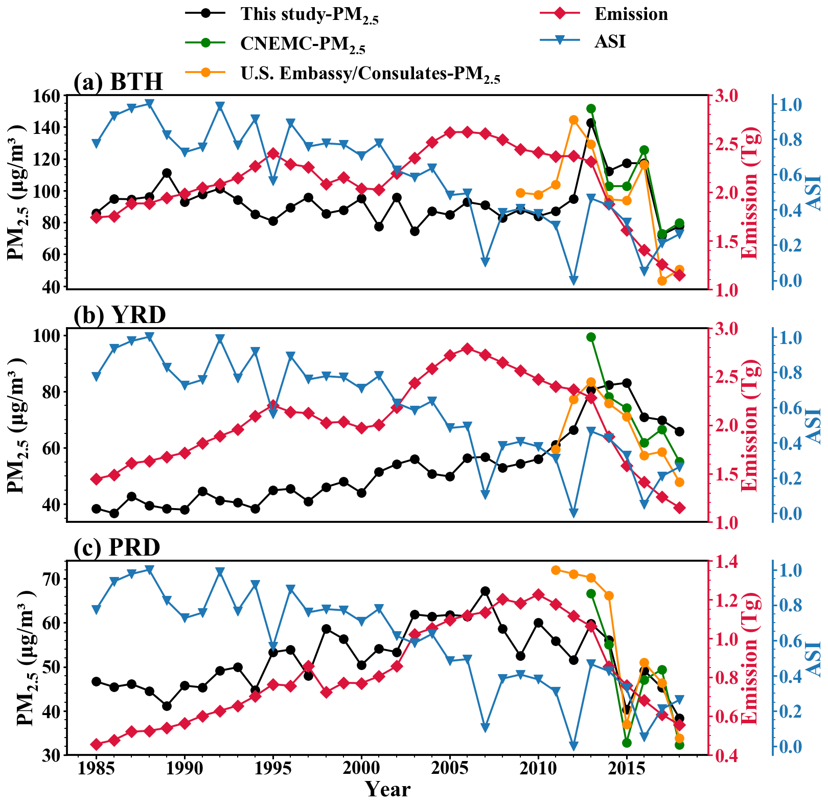
Figure 1Annual winter averages of retrieved PM2.5 concentrations (black, 1985–2018), emission (red, 1985–2018), and Arctic sea ice (ASI, blue, 1985–2018) in BTH, YRD, and PRD; PM2.5 concentrations observed by the US Embassy and consulates in Beijing (orange, 2009–2018) and Shanghai and Guangzhou (orange, 2011–2018); PM2.5 concentrations observed by CNEMC (green, 2013–2018).
2.1 Data
Winter visibility data in 1973–2019 are obtained from Global Surface Summary of the Day (GSOD) data provided by the National Climatic Data Center (NCDC) (https://www.ncei.noaa.gov/maps/daily/, last access: 10 March 2022). The relative humidity (RH) is derived from dew point temperature and air temperature of GSOD following the approach proposed by Lawrence (2005). Surface PM2.5 measurements in 2013–2019 are taken from the China National Environment Monitoring Center (CNEMC, http://www.cnemc.cn/, last access: 10 March 2022). The PM2.5 concentrations were measured by the micro-oscillating balance method and/or the β-absorption method (MEE, 2012; Zhang and Cao, 2015). The autumn (September–October–November) Arctic sea ice (ASI) index is defined as the normalized sea ice fraction north of 45∘ N as suggested by Wang et al. (2015), which is calculated from the Hadley Centre (HadISST1 – Hadley Centre Sea Ice and Sea Surface Temperature data set, https://www.metoffice.gov.uk/hadobs/hadisst, last access: 10 March 2022) with 1∘ × 1∘ resolution for 1870–2022 (Rayner et al., 2003).
PM emission inventories of PM10, PM2.5, SO2, NH3, NOx, black carbon, and organic carbon in this study are obtained from Peking University (PKU, 1960–2014, 0.1∘ × 0.1∘, monthly), which include the fuel consumption and emissions of greenhouse gases and air pollutants from all combustion sources (http://inventory.pku.edu.cn/, last access: 10 November 2021). The Multi-resolution Emission Inventory for China (MEIC, version 1.3, 2010–2017, 0.25∘ × 0.25∘, monthly, http://www.meicmodel.org, last access: 10 November 2021; Li et al., 2017; Zheng et al., 2018) provided by Tsinghua University and the PRD emission inventory (PRD-EI, 2006–2019, 3∘ × 3∘, monthly) from Huang et al. (2021) and Zhong et al. (2018) are also used. Due to the discontinuity of these three inventories, we calculate the scaling factor of each pollutant based on the overlapping period to obtain a winter inventory from 1985–2018 (Fig. 1) in PRD as follows:
where Ei is emission of species i; the subscripts PKU and PRD-EI denote the PKU inventory and the PRD inventory of Huang et al. (2021) and Zhong et al. (2018), respectively; and j denotes year.
The corresponding formulas for BTH and YRD are
where the subscript MEIC denotes the MEIC inventory.
Since the ratios of annual emission inventories in PRD to those of YRD and BTH are not expected to change significantly in 1 or 2 years (Fig. S1 in the Supplement), the 2016 winter emission ratio of BTH to PRD is multiplied by the 2017 and 2018 winter emission of PRD to obtain the winter emission of BTH in 2017 and 2018. The same is true for 2017 and 2018 winter emission of YRD. The annual emission inventories for BTH, YRD, and PRD from 1985 to 2018 are shown in Fig. 1. It should be noted that the winter of a specific year in this study includes December of this year and January and February of the following year.
2.2 Nonlinear exponential fitting
Since directly observed data of PM2.5 are not available before 2013, we employ nonlinear exponential fitting to retrieve PM2.5 concentrations in BTH, YRD, and PRD from visibility data that have a long-term and complete record. Because RH affects strongly the relationship between PM2.5 concentration and visibility (Fu et al., 2016; Liu et al., 2017; L. Zhang et al., 2015; Q. Zhang et al., 2015), we evaluate the relationship for different RH intervals in each region as shown in Figs. S2–S4. The r2 of average fitting is greater than 0.50, sometimes as high as 0.77, significant at a 99 % confidence level, indicating that the fitting performance is acceptable (Figs. S2–S4). As expected, the retrieved PM2.5 has a significant negative correlation with visibility (Fig. S5). More importantly, the retrieved PM2.5 concentrations are in good agreement with the observed PM2.5 in recent years from CNEMC (2013–2018) and those observed in the US Embassy in Beijing (2009–2018) and consulates in Shanghai and Guangzhou (2011–2018) (Fig. 1). Since the embassy–consulates PM2.5 data are totally independent of the retrieving of PM2.5 concentrations from visibility, the agreement between our retrieved PM2.5 concentrations and those observed in the US Embassy in Beijing and consulates in Shanghai and Guangzhou lends strong support to the validity of our retrieved PM2.5 concentrations.
A quick inspection of the PM2.5 and emission lines in Fig. 1 reveals that an expected good regression between PM2.5 and emission is only possible for PRD where the emission line matches well with the PM2.5 line in general as both have a broad maximum near 2005–2010 (Fig. 1c). In BTH a good regression is made difficult due to a critical mismatch characterized by two broad maxima (1985–2000, 2000–2013) in the emission line and a sharp drop after 2013, while the PM2.5 line has a shallow depression during the period 1993–2012 followed by a large bulge that peaked in 2013 (named hereafter as bulge-2013) and lasted until 2016 (Fig. 1a). This mismatch also existed in YRD as the emission line crossed over the PM2.5 line in opposite directions near 2012, although the bulge was not as large and a depression could barely be seen in 2003–2012 (Fig. 1b).
Mao et al. (2019) analyzed extensively the depression of 1999–2012 (the deeper part of the 1993–2012 depression) and bulge-2013. They found that the depression and bulge-2013 were primarily caused by a combination of climate oscillations which include negative phases of the Pacific Decadal Oscillation, Arctic Oscillation, El Niño–Southern Oscillation, and global temperature, in addition to positive phases of the East Asian winter monsoon and ASI. It is clear that the presence of bulge-2013 can have a big impact on any study on the contributions of meteorology/climate and anthropogenic emission control to the linear trends in PM2.5, especially for a short-term study such as the period 2013–2018 that overlooks the cause of the bulge. This point will be elaborated in Sect. 3.3 and 3.4. Finally, given the critical importance of bulge-2013, it is reassuring that the existence of bulge-2013 is independently confirmed by the PM2.5 concentrations retrieved from visibility as well as those observed in the US Embassy in Beijing and consulate in Shanghai.
3.1 Multiple linear regression studies
Zhai et al. (2019) constructed a stepwise MLR model to quantify the meteorological contribution to the PM2.5 trends. The MLR model made correlation analysis between the 10 d PM2.5 anomalies and wind speed, precipitation, RH, and temperature, as well as 850 hPa meridional wind velocity. The residual after removing meteorological influence from the MLR model was considered to be driven by changes in anthropogenic emissions. The authors quantified the contribution of meteorology to PM2.5 trends from 2013 to 2018 in BTH, YRD, and PRD at 14 %, −3 %, and 19 %, respectively. The residuals, 86 %, 103 %, and 81 %, of PM2.5 trends were attributed to anthropogenic emissions (Table 1).
Table 1Comparison of the contribution of emissions and meteorological conditions to the observed PM2.5 trends in 2013–2018 (2013–2017 for Chen et al., 2019).
KZ: Kolmogorov–Zurbenko filter; MLR: stepwise multiple linear regression; MLR-EMIS indicates the use of emissions and PM2.5 as inputs to the MLR model.
Chen et al. (2019) employed a Kolmogorov–Zurbenko (KZ) filter to produce an adjusted long-term time series of PM2.5 concentrations in Beijing from 2013 to 2017 by removing interannual and seasonal variations in meteorological conditions. They applied MLR models between PM2.5 and wind speed, RH, temperature, and solar radiation to remove the influence of meteorological conditions and estimated that the contribution of emissions to adjusted PM2.5 was 81 %, while the contribution of meteorology was 19 % (Table 1).
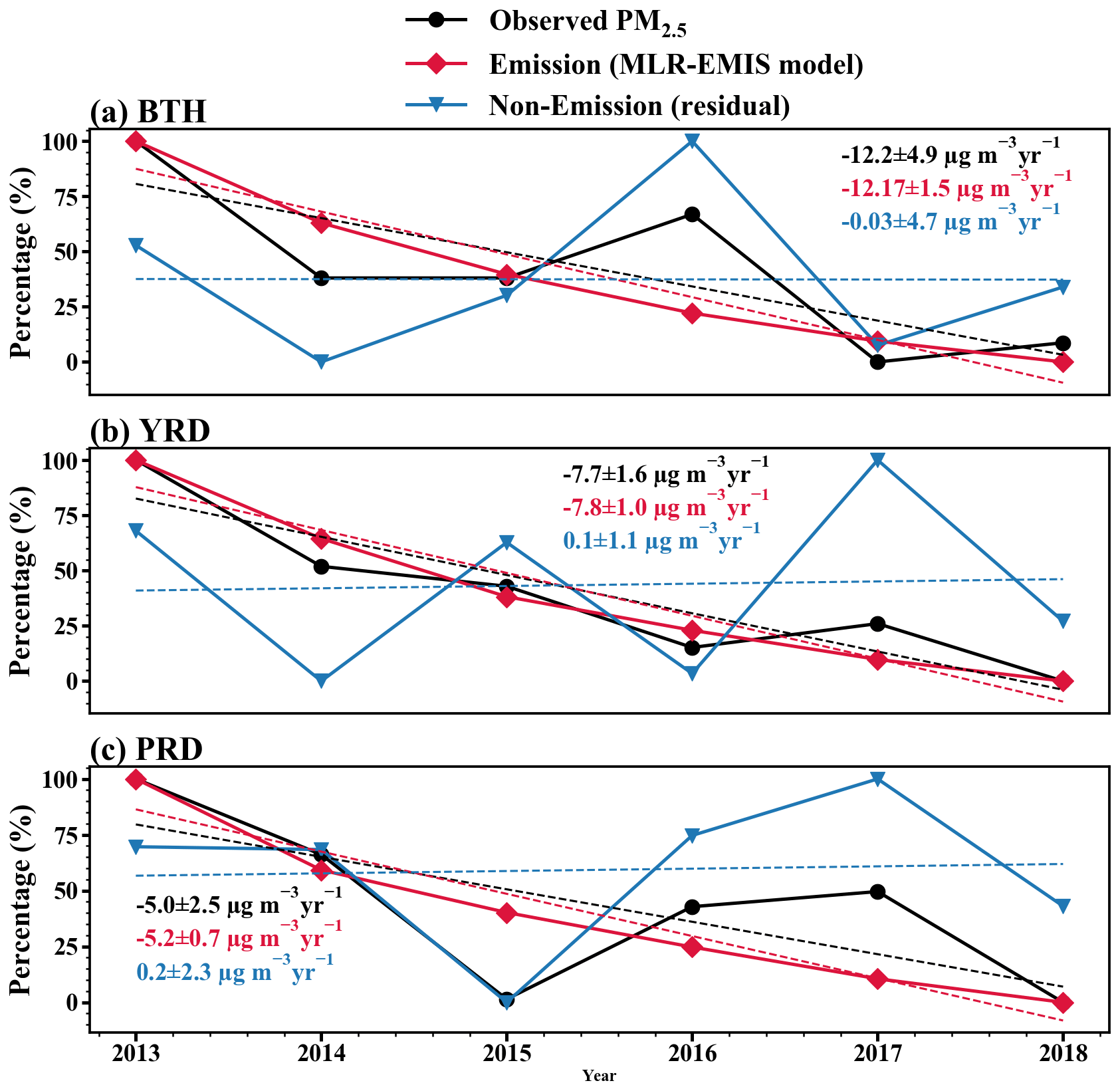
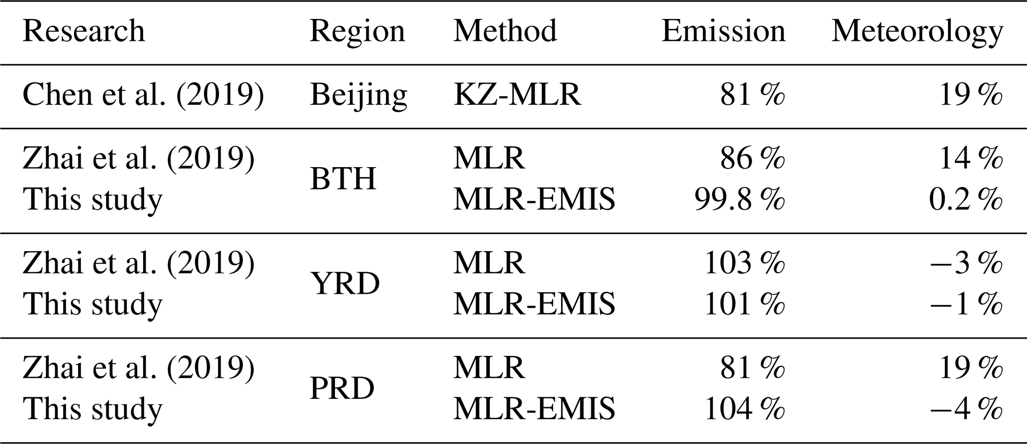
Figure 2Results of MLR-EMIS analysis for 2013–2018 in BTH (a), YRD (b), and PRD (c). Temporal variations in observed winter PM2.5 concentration are shown in black; contributions of anthropogenic emissions to the PM2.5 trend are shown in red; and the residual is shown in blue. Values inset in each panel are the ordinary linear regression trends, with 95 % confidence intervals obtained by Student's t test.
To compare with these two studies, we carry out an MLR analysis of the emission and observed concentrations of PM2.5, of which the results will be denoted hereafter as MLR-EMIS. As shown in Fig. 2, the observed PM2.5 decreased remarkably from 2013 to 2018 in the three regions, with a downward trend of −12.2 in BTH, −7.7 in YRD, and −5.0 in PRD. The MLR-EMIS model can mostly capture these decreasing features. The non-emission (residual) in BTH, YRD, and PRD has a trend of −0.03, 0.1, and 0.2 , respectively, or 0.2 %, −1.0 %, and −4.0 %, respectively, of the observed trends. Hence, the contribution of climate/meteorology to the observed linear trend in winter PM2.5 in BTH, YRD, and PRD from 2013 to 2018 is 0.2 %, −1.0 %, and −4.0 %, respectively, meaning that 99.8 %, 101.0 %, and 104.0 % of the linear trend in the observed winter PM2.5 is attributable to emission (Table 1). These results of MLR-EMIS regarding the predominant contribution of emission are in good agreement with Zhai et al. (2019) and Chen et al. (2019). This agreement is reinforced by a mechanistic model assessment conducted by Chen et al. (2019), who suggested that the contribution of emissions to the linear trend in PM2.5 in 2013–2017 was 79 %, while the contribution by meteorology was only 21 %. In addition, Gong et al. (2021) developed a framework based on an environmental meteorology index to quantitatively assess the contribution of meteorology variations to the trend of PM2.5 concentrations and separate the impacts of meteorology from the emission-control measures. They found that emission control contributed more than 90 % of the PM2.5 trend in BTH from 2013 to 2017, again in good agreement with those values in BTH and Beijing shown in Table 1 (upper two rows).
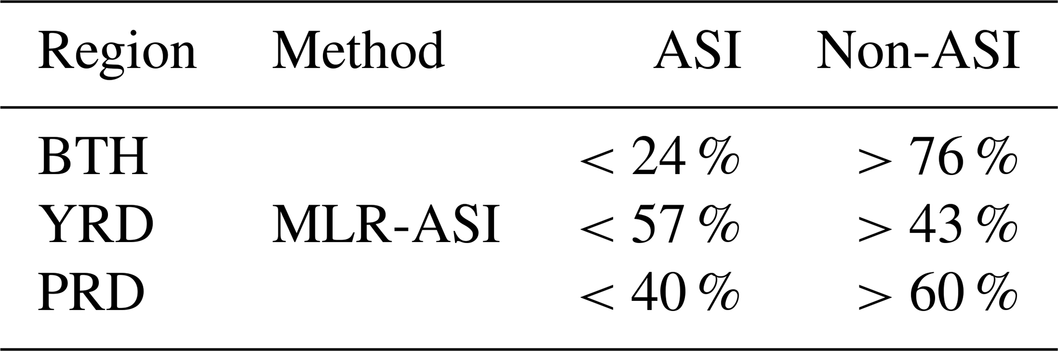
Wang et al. (2015) hypothesized that the decreasing ASI could be an important contributor to the recent increase in haze days in eastern China, and about 45 %–67 % of the interannual to interdecadal variability in winter haze days could be explained by the ASI variability. Following the MLR-EMIS model study above, we carry out a parallel MLR-ASI model study in which the emission is replaced by ASI (Fig. 3). The non-ASI trends (residuals) contribute −9.3, −3.3 and −3.0 , respectively, to the observed linear trends in winter PM2.5 in BTH, YRD and PRD, which imply that the emissions (non-ASI) are responsible for 76 %, 43 % and 60 % of the observed linear trend in winter PM2.5 in BTH, YRD and PRD, respectively, in 2013–2018 (Table 2). It follows that ASI can explain 24 %, 57 %, and 40 % of the decreasing trends in BTH, YRD, and PRD, respectively (Table 2), which are on the low side but nevertheless in qualitative agreement with Wang et al. (2015). Here we note that the contribution of ASI represents only a partial contribution of climate/meteorological conditions; adding other meteorological parameters would increase the contribution.
Table 2Contributions of Arctic sea ice (ASI) and residuals (non-ASI) to the observed PM2.5 trends in the winter seasons of 2013–2018.

Note: MLR-ASI indicates the use of ASI and PM2.5 as inputs to the MLR model.
The comparison of Tables 1 and 2 poses an interesting problem. For BTH, the MLR-ASI value of 76 % (Table 2) for the contribution of emissions is slightly lower than, but nevertheless agrees qualitatively with, the results of MLR-EMIS in the upper two rows of Table 1. However, for YRD and PRD, the contributions of 43 % and 60 % (Table 2), respectively, by non-ASI (including emissions) to the observed linear trends in winter PM2.5 are significantly less than those values of 101 %–104 % derived by the MLR-EMIS analysis (bottom two rows of Table 1). What causes the discrepancy? Which table has the correct results? The answer to the first question is that there were significant linear trends in PM2.5, anthropogenic emissions, and ASI in 2013–2018 (Figs. 1 and 3), but there was no significant linear trend in 2013–2018 in the meteorological parameters used in the studies by Zhai et al. (2019) and Chen et al. (2019). The MLR analysis gives high values to correlation coefficients of parameters with significant linear trends. In fact, any parameter with a significant linear trend in 2013–2018, e.g., sea surface temperature (SST) of the western Pacific, would get a high correlation coefficient in the MLR analysis.
3.2 Comparing the MLR results to mechanistic models
The answer to the question of whether Table 1 or 2 is correct is that neither of them is correct, for the following reasons: all evaluations in Tables 1 and 2 quantified the contributions of anthropogenic emission and meteorology to the linear trend of PM2.5 in 2013–2018 using certain statistical MLR models. No mechanistic process was considered in these models. This raises a fundamental concern about the attribution of causes based on statistical regression results alone. It is well known that a good correlation in the MLR analysis does not imply any causal relationship. The causal relationship can only be established if a mechanistic model that simulates the atmospheric environment with realistic emissions of air pollutants and ambient meteorological conditions as model inputs can credibly reproduce the observed concentrations and trends of PM2.5. Therefore, we conclude that the quantitative results in Tables 1 and 2 are not scientifically credible unless corroborated by a mechanistic model.
The KZ-MLR results of Chen et al. (2019) in Table 1 were corroborated by the Weather Research and Forecasting and the Community Multiscale Air Quality model (WRF-CMAQ), a mechanistic model (Chen et al., 2019). However, the mechanistic model study of Chen et al. (2019) consisted of short-term (2013–2017) simulations. As noted in Sect. 2.2, a short-term study of 2013–2017 overlooks the effect and the cause of bulge-2013, which might lead to significant uncertainties and/or biased results. In this context, we believe that a credible mechanistic (or MLR) model study should cover a long enough time before the period of interest (2013–2018) so that the model could be constrained by the major features of interannual variations such as bulge-2013 and the depression before it (Fig. 1a).
We summarize the discussions involving Tables 1 and 2 as follows. (1) Quantitative MLR results in Tables 1 and 2 without corroboration by a mechanistic model are not credible. (2) Results from mechanistic models are more credible than MLR in theory, but significant uncertainties and/or biased results exist in the short-term model simulations.
3.3 An alternative interpretation of MLR results
In view of the difficulty in interpreting the results from MLR analysis, we propose an alternative interpretation of the correlation coefficient by interpreting it as “the maximum possible contribution of an independent variable (e.g., emissions in Table 1) to the dependent variable (e.g., linear trends of PM2.5 in Table 1)”, while the residual should be interpreted as the minimum contribution of all other independent variables (e.g., non-emission variables such as meteorological parameters in Table 1). A theoretical foundation in support of this alternative interpretation can be understood as follows: the MLR analysis is, in effect, performing an optimum fit between the independent variable and the dependent variable. In other words, the optimum fit enables the independent variable (e.g., emission in our case) to attain the optimum/maximized contribution to the variability (including the linear trend) of the dependent variable (e.g., PM2.5). Furthermore, the maximum possible contribution in the alternative interpretation is reinforced because all factors other than emission (e.g., ASI) that may contribute to the variability (including the linear trend) are excluded in the optimum-fit process.
Table 3Contributions of emissions and non-emissions (including climate and meteorological conditions) to the observed PM2.5 trends in 2013–2018 (2013–2017 for Chen et al., 2019).
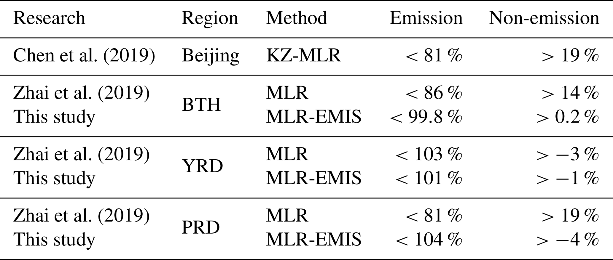
Table 4Contributions of ASI and residuals (non-ASI) to the observed PM2.5 trends in 2013–2018.
Tables 3 and 4 are the corresponding outcomes from the new interpretation for Tables 1 and 2, respectively. It is clear that under the new interpretation, Tables 3 and 4, unlike Tables 1 and 2, are now consistent with each other. In addition, the results of Chen et al. (2019) and Gong et al. (2021), under the new interpretation, are also consistent with the range of values in Tables 3 and 4. These consistent results provide a solid cornerstone to explore additional applications of the alternative interpretation as discussed in Sect. 3.4.
Table 5Contributions of emissions and ASI to the PM2.5 trends in BTH.

Note: the superscripts obs and ret indicate the use of observed and retrieved PM2.5 data, respectively. Superscript ret34 indicates the retrieved PM2.5 data for 2013–2018 obtained using the data of 1985–2018.
Another critical factor affecting the MLR results is the length of time period studied. Table 5 compares the results of two short-term studies (2013–2017, 2013–2018) in BTH to a long-term study (1985–2018) for MLR-EMIS and MLR-ASI. The emissions of MLR-EMIS can contribute to a maximum of 101 % of the observed trend of PM2.5 in BTH during 2013–2017, while the residual parameters contribute at least −1 %. For the MLR-ASI analysis, the maximum possible contribution of ASI to observed PM2.5 in 2013–2017 is 30 %, while the residuals (including emissions) contribute at least 70 %. Using the retrieved PM2.5 does not change the results significantly from the observed PM2.5. Adding 2018 into consideration makes little difference for MLR-EMIS. However, adding only the year 2018, the ASI's maximum possible contribution to observed PM2.5 declines by about 11 % compared to that of 2013–2017, while the minimum contribution of the residual increases from 57 % to 68 % (Table 5). The reason for the larger change in the MLR-ASI can be readily understood by comparing the solid red line (EMIS) in Fig. 2a to that (ASI) of Fig. 3a: the former maintained a smooth declining trend in 2016–2018, while the latter turned around and increased from 2016 to 2018. This turning around made the MLR-ASI regression significantly worse and was responsible for the residual increasing from 57 % to 68 %.
Table 6Contributions of emissions and ASI to the PM2.5 trends in YRD.
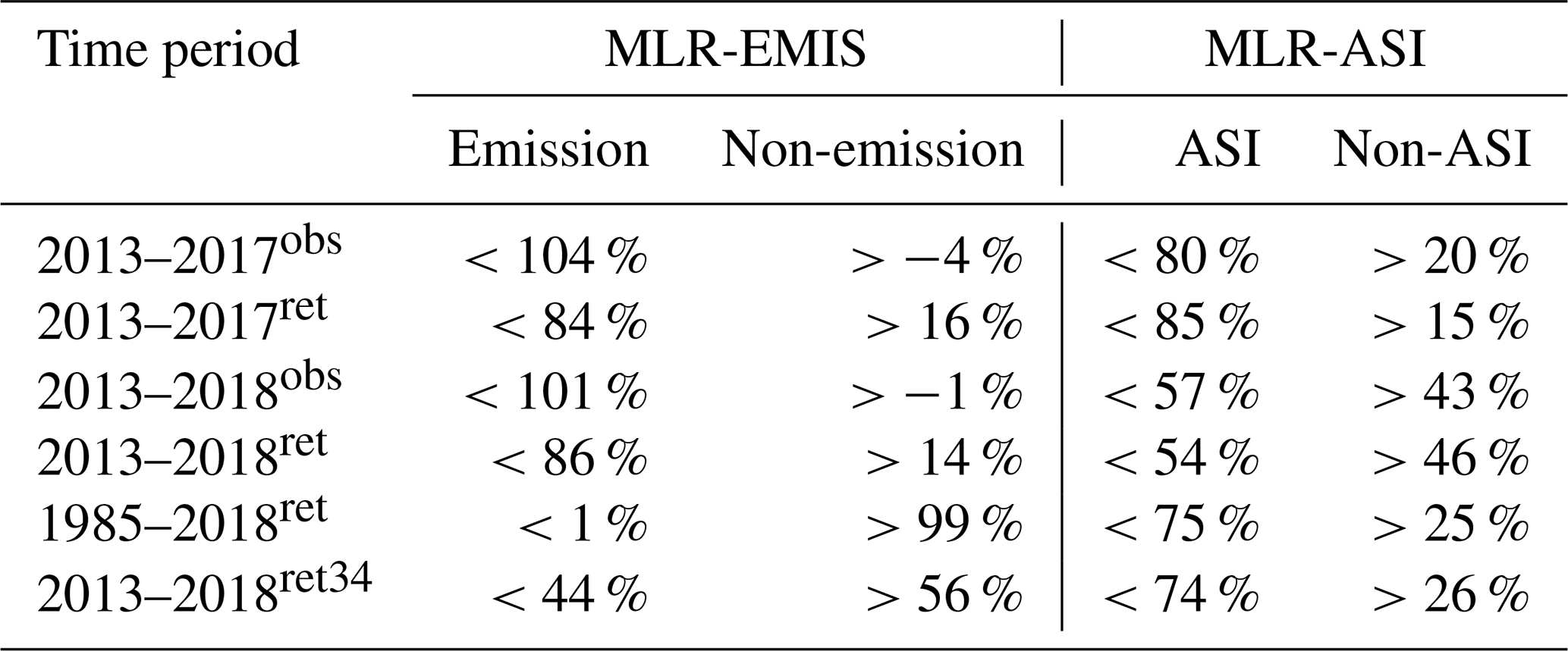
Table 7Contributions of emissions and ASI to the PM2.5 trends in PRD.
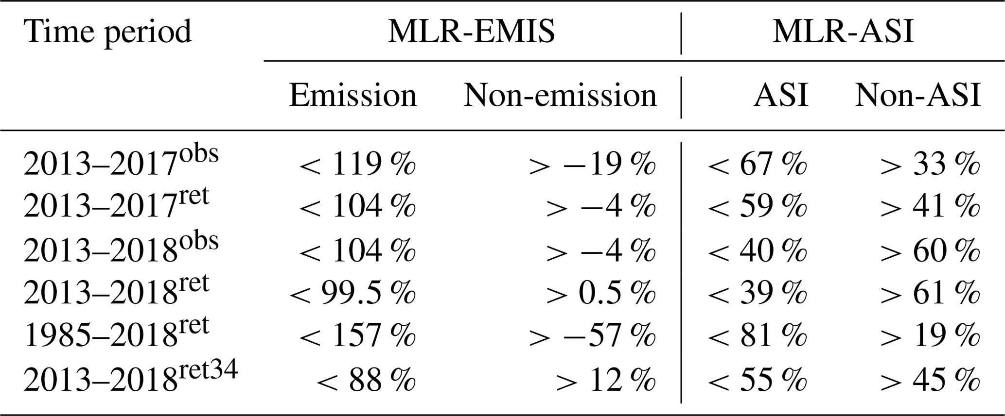
The 2013–2017 and 2013–2018 results of MLR-EMIS in YRD (Table 6) and PRD (Table 7) were also consistent with those in BTH (Table 5). The 2013–2017 and 2013–2018 results of MLR-ASI in PRD were consistent with those in BTH, while the values of corresponding results of YRD were relatively large compared with the other two regions. The reason for the difference was that the solid red line (ASI) and the solid black line (observed PM2.5) in YRD showed relatively consistent trends from 2013 to 2017, while both lines showed opposite trends in the 2014–2017 BTH and 2015–2018 PRD (Fig. 3). The consistent trend between the two lines made the MLR-ASI regression in YRD relatively good, resulting in the maximum contribution of ASI to PM2.5 in YRD from 2013 to 2017 being 80 %, while the residual contribution was greater than 20 %. After adding the opposite upward trend of the two curves from 2017 to 2018, the maximum ASI contribution to PM2.5 in YRD decreased substantially from 85 % to 54 %, while the residual increased to >46 % (Table 6).
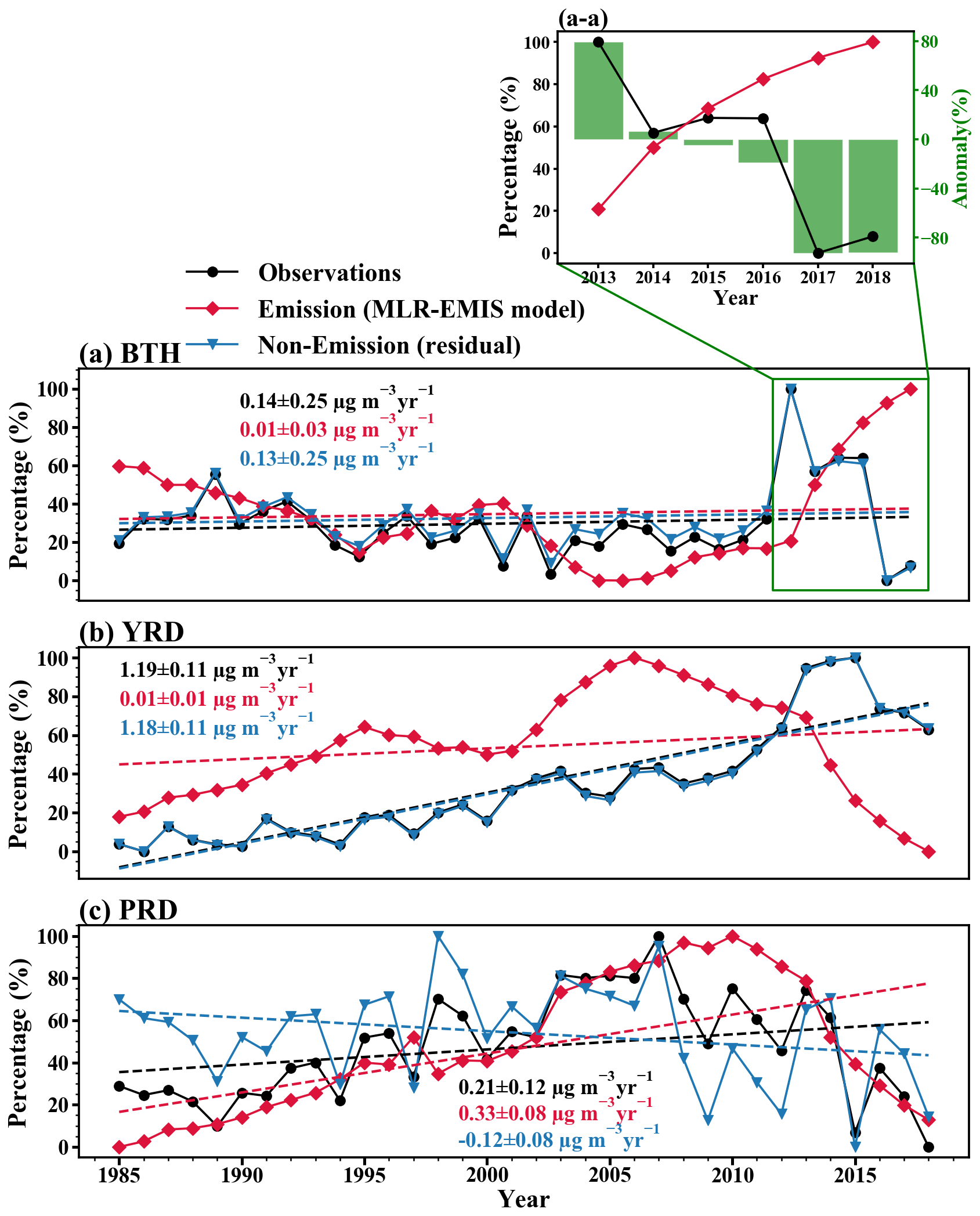
Figure 4The same as Fig. 2 but for time period of 1985–2018. Panel (a-a) shows enlarged schematic representations of the period 2013–2018 in panel (a).
Extending to 1985–2018, these long-term results differed drastically from the short-term results: the contribution of emissions in MLR-EMIS to the linear trends of PM2.5 in BTH for the 34-year study was merely <7 %, while the contribution of all residual parameters was >93 %. The small upper limit of 7 % can be easily explained by examining Fig. 4a, in which the regression between the red line (emission) and black line (PM2.5) is very poor, especially after 2010 when the observed PM2.5 started to climb from around 20 % to the bulge-2013 of 100 %. In fact, the red emission line in Fig. 1a had to be turned upside down in Fig. 4a to obtain the best fit to the black line of PM2.5 (note the fit between 1988 and 2012 was fairly good), which resulted in the red line to miss bulge-2013 completely. The small contribution of emissions compared to the residuals is in good agreement with the mechanistic model results of Dang and Liao (2019) who found that meteorology contributed significantly more than emissions to the linear trend as well as the interannual variability in severe winter haze days in BTH in 2013–2017. The MLR-ASI analysis for PM2.5 in BTH over the 34-year period from 1985 to 2018 had a slightly better regression result as shown in Fig. 5a. As a result, the maximum possible contribution of ASI to the linear trend of PM2.5 was 43 %, while the minimum contribution of the residuals was 57 % (Table 5). Bulge-2013 in the winter haze days in the North China Plain was also noticed by Yin and Wang (2017), whose generalized additive model using ASI and SST as predictors was found to capture the interannual and interdecadal variations in winter haze days in 1980–2015, including bulge-2013.

For YRD, the 1985–2018 emission contribution to the linear trend in the observed PM2.5 had an upper limit of only 1 %, implying the contribution of residuals (including meteorology) to be at least 99 % (Table 6). The small 1 % can be explained by the extremely poor match between the red line (emission) and the black line (PM2.5) in Fig. 4b. The regression result of the MLR-ASI analysis in YRD was relatively good. Although the red line (ASI) also failed to match bulge-2013, it matched well with the 2016–2018 profile as shown in Fig. 5b. As a result, the maximum possible contribution of ASI to the 34-year linear trend of PM2.5 reached 75 %, implying the minimum contribution of the residuals was 25 % (Table 6). PRD did not have bulge-2013 (Fig. 1c) and therefore had a good regression between emissions and PM2.5 from 1985 to 2018 (Fig. 4c), implying that emissions over the 34-year period could contribute as much as 157 % to the linear trend of PM2.5, while % was contributed by the residuals (Table 7). The regression result of the MLR-ASI analysis for PM2.5 in PRD from 1985 to 2018 was slightly better than those of the MLR-EMIS, and the red line (ASI) and the black line (PM2.5) showed opposite trends only in 2011–2015, as shown in Fig. 5c, resulting in the maximum contribution of ASI to the linear trend of PM2.5 being 81 %, while the minimum contribution of the residuals was 19 % (Table 7).
3.4 Best estimate of the contribution
Tables 5–7 and Figs. 4–5 provide strong evidence supporting the notion that the contributions of emissions and meteorology to the linear trend in PM2.5 depend on the length of time analyzed. A critical question remaining is which regression analysis gives the correct value of the contribution when a long-term analysis overlaps with a short-term analysis, e.g., the 1985–2018ret analysis (Fig. 4a) vs. the 2013–2018ret analysis (Fig. 2a) for BTH during the period 2013–2018 (fourth row vs. last row in Table 5). A logical answer to this question is that the long-term analysis gives the correct value because it has more data points to constrain the regression. This is discussed in the following using the BTH case as an example.
Figure 4a-a shows an enlarged plot of the 2013–2018 portion of Fig. 4a (named as 2013–2018ret34 analysis hereafter and in Tables 5–7). The solid green bars in Fig. 4a-a denote the anomalies/deviations of the red emission line from the black observation line, of which the mean absolute value of 49 % (third column and the last row of Table 5) can be recognized as the minimum contribution of the residual/non-emission (including meteorology/climate) to the linear trend in PM2.5 according to the alternative interpretation. Hence the maximum possible contribution by EMIS is 51 %, which is substantially less than the 94 % of the 2013–2018ret analysis (second column and fourth row of Table 5). The main reason for this difference can be traced to bulge-2013 in Fig. 4a, which, as discussed in Sect. 3.3, contributes pivotally to the red emission line in Fig. 1a being turned upside down in Fig. 4a to obtain the best fit with the black line of observed PM2.5. For the 2013–2018ret34 ASI analysis, the solid green bars of Fig. 5a-a denote the anomalies/deviations of ASI line from the PM2.5 line, of which the mean absolute value of 38 % (fifth column and last row of Table 5) can be recognized as the minimum contribution of the residual of ASI, which includes emissions. Hence, we derive the maximum possible contribution by ASI to be 62 % (fourth column and last row of Table 5). Key results of the two analyses above are summarized in the fourth and last rows of Table 5. Qualitatively the results of the 2013–2018ret analysis and the 2013–2018ret34 analysis are consistent (overlap) with each other; quantitatively a significant difference exists between the two analyses: the contribution of emission to the linear trend in PM2.5 in the latter has a tighter upper limit of only 51 % compared to 94 % of the former and a greater lower limit for the contribution of the residual which includes meteorology/climate in the latter (49 %) compared to the former (6 %). The fact that the long-term analysis renders a tighter upper/lower limit is evidently the result of additional constraints provided by the long-term data. Finally, since a tighter upper/lower limit gives a more precise estimate of the contribution, we propose that the best estimates of the contributions of emission, ASI, and other meteorology/climate parameters to the linear trend in PM2.5 in BTH during 2013–2018 are those listed in the last row of Table 5, specifically, emission <51 %, non-emission >49 %, ASI <62 %, and non-ASI >38 %. These are our best estimates and are remarkably different from those of MLR studies listed in Table 1.
The same analysis can be carried out for YRD and PRD, and the key results are summarized in the fourth and last rows of Tables 6 and 7, respectively. For YRD, the best estimates of the contributions of emission, ASI, and other meteorology/climate parameters to the linear trend in PM2.5 during 2013–2018 are those listed in the last row of Table 6, specifically, emission <44 %, non-emission >56 %, ASI <74 %, and non-ASI >26 %. For PRD, the best estimates of the contributions of emission, ASI, and other meteorology/climate parameters to the linear trend in PM2.5 during 2013–2018 are those listed in the last row of Table 7, specifically, emission <88 %, non-emission >12 %, ASI <55 %, and non-ASI >45 %. These best estimates are also significantly different from those of MLR studies listed in Table 1.
Recently, Chen et al. (2019) and Zhai et al. (2019) used MLR models to analyze the significant downward trend of PM2.5 concentrations in China's major air pollution regions in 2013–2018 (2013–2017 for Chen et al., 2019) and quantified that the control of anthropogenic emissions accounted for 81 % to 103 % of the PM2.5 reduction (Table 1). While there is little doubt that anthropogenic emissions make a significant contribution to the reduction trend of PM2.5, we are skeptical of these high contributions by emissions obtained based solely on MLR models because a good correlation in MLR analysis does not imply any causal relationship. In this regard, Chen et al. (2019) corroborated their MLR result of 81 % (Table 1) using the mechanistic model WRF-CMAQ. However, the mechanistic model study of Chen et al. (2019) consisted of short-term (2013–2017) simulations. As noted in Sect. 2.2, a short-term study of 2013–2017 overlooked the effect and the cause of bulge-2013, which could lead to significant uncertainties and/or biased results. In this context, we believe that a credible mechanistic (or MLR) model study should cover a long enough time before the period of interest (2013–2017) so that the model could be constrained by the major features of interannual variations such as bulge-2013 and the depression before it (Fig. 1a).
To compare with previous MLR studies, the MLR model is used in this study to assess the contributions of climate/meteorology and anthropogenic emissions to the linear trends of PM2.5 concentration in three regions in eastern China, namely BTH, YRD, and PRD. We first carry out an MLR analysis (MLR-EMIS) on the emissions and observed trend of PM2.5 in BTH during 2013–2018 and show that the results of Zhai et al. (2019) and Chen et al. (2019) can be satisfactorily reproduced (Table 1). Then the same MLR analysis is performed on ASI and the observed trend of PM2.5 (MLR-ASI), and we obtain a 76 % contribution by emissions in BTH, which is slightly lower than, but nonetheless in qualitative agreement with, those values obtained by Zhai et al. (2019) and Chen et al. (2019) (Tables 1 and 2). However, for YRD and PRD, the contributions of emissions to the observed trends of PM2.5 are only 43 % and 60 % (Table 2), respectively, significantly less than those values of 101 %–104 % derived by the MLR-EMIS analysis (Table 1). We believe that the discrepancy is rooted in the false assumption/interpretation of the correlation coefficient as the value of contribution in the MLR studies as discussed earlier. We therefore propose an alternative interpretation: the correlation coefficient should be interpreted as the maximum possible contribution of the independent variable to the dependent variable, and the residual should be interpreted as the minimum contribution of all other independent variables. Under the new interpretation, all previous results as shown in Tables 3–4 become consistent with one another.
Another important outcome from this study is that the results of a short-term (2013–2018) analysis are significantly different from those of a long-term (1985–2018) analysis for the period 2013–2018 in which they overlap, suggesting that MLR results depend critically on the length of time analyzed. The long-term analysis renders a more precise estimate because of additional constraints provided by the long-term data. We therefore suggest that the best estimates of the contributions of emissions and non-emission (including climate/meteorology) to the linear trend in PM2.5 during 2013–2018 are those from the long-term analyses: i.e., emission <51 % and non-emission >49 % for BTH, emission <44 % and non-emission >56 % for YRD, and emission <88 % and non-emission >12 % for PRD.
Visibility data were obtained from Global Surface Summary of the Day (GSOD) data provided by the National Climatic Data Center (NCDC) (https://www.ncei.noaa.gov/maps/daily/, last access: 10 March 2022). Surface PM2.5 measurements from 2013–2019 are taken from China National Environment Monitoring Center (CNEMC, http://www.cnemc.cn/, last access: 10 March 2022). The data of this paper are available upon request to Shaw Chen Liu (shawliu@jnu.edu.cn).
The supplement related to this article is available online at: https://doi.org/10.5194/acp-22-11945-2022-supplement.
RL and SCL proposed the essential research idea. YW performed the analysis. YW, RL, and SCL drafted the manuscript. JD, YL, ZH, and JZ helped with analysis and offered valuable comments. All authors have read and agreed to the published version of the paper.
The contact author has declared that none of the authors has any competing interests.
Publisher's note: Copernicus Publications remains neutral with regard to jurisdictional claims in published maps and institutional affiliations.
The authors thank the National Climatic Data Center (NCDC) and the China National Environmental Monitoring Center for providing data sets that made this work possible. We also acknowledge the support of the Institute for Environmental and Climate Research and Guangdong–Hong Kong–Macau Joint Laboratory of Collaborative Innovation for Environmental Quality, Jinan University.
This research has been supported by the National Natural Science Foundation of China (grant nos. 92044302 and 41805115), the Guangzhou Municipal Science and Technology Project (grant no. 202002020065), the Special Fund Project for Science and Technology Innovation Strategy of Guangdong Province (grant no. 2019B121205004), and the Guangdong Innovative and Entrepreneurial Research Team Program (grant no. 2016ZT06N263).
This paper was edited by Veli-Matti Kerminen and reviewed by three anonymous referees.
Albrecht B. A.: Aerosols, cloud microphysics, and fractional cloudiness, Science, 245, 1227–1230, https://doi.org/10.1126/science.245.4923.1227, 1989.
Carslaw, K. S., Boucher, O., Spracklen, D. V., Mann, G. W., Rae, J. G. L., Woodward, S., and Kulmala, M.: A review of natural aerosol interactions and feedbacks within the Earth system, Atmos. Chem. Phys., 10, 1701–1737, https://doi.org/10.5194/acp-10-1701-2010, 2010.
Chen, Z., Chen, D., Kwan, M.-P., Chen, B., Gao, B., Zhuang, Y., Li, R., and Xu, B.: The control of anthropogenic emissions contributed to 80 % of the decrease in PM2.5 concentrations in Beijing from 2013 to 2017, Atmos. Chem. Phys., 19, 13519–13533, https://doi.org/10.5194/acp-19-13519-2019, 2019.
Cohen, A. J., Brauer, M., Burnett, R., Anderson, H. R., Frostad, J., Estep, K., Balakrishnan, K., Brunekreef, B., Dandona, L., and Dandona, R.: Estimates and 25-year trends of the global burden of disease attributable to ambient air pollution: an analysis of data from the Global Burden of Diseases Study 2015, The Lancet, 389, 1907–1918, https://doi.org/10.1016/S0140-6736(17)30505-6, 2017.
Dang, R. and Liao, H.: Severe winter haze days in the Beijing–Tianjin–Hebei region from 1985 to 2017 and the roles of anthropogenic emissions and meteorology, Atmos. Chem. Phys., 19, 10801–10816, https://doi.org/10.5194/acp-19-10801-2019, 2019.
Fu, X., Wang, X., Hu, Q., Li, G., Ding, X., Zhang, Y., He, Q., Liu, T., Zhang, Z., Yu, Q., Shen, R., and Bi, X.: Changes in visibility with PM2.5 composition and relative humidity at a background site in the Pearl River Delta region, J. Environ. Sci., 40, 10–19, https://doi.org/10.1016/j.jes.2015.12.001, 2016.
Gong, S., Liu, H., Zhang, B., He, J., Zhang, H., Wang, Y., Wang, S., Zhang, L., and Wang, J.: Assessment of meteorology vs. control measures in the China fine particular matter trend from 2013 to 2019 by an environmental meteorology index, Atmos. Chem. Phys., 21, 2999–3013, https://doi.org/10.5194/acp-21-2999-2021, 2021.
Han, X., Zhang, M., Gao, J., Wang, S., and Chai, F.: Modeling analysis of the seasonal characteristics of haze formation in Beijing, Atmos. Chem. Phys., 14, 10231–10248, https://doi.org/10.5194/acp-14-10231-2014, 2014.
Huang, Z., Zhong, Z., Sha, Q., Xu, Y., Zhang, Z., Wu, L., Wang, Y., Zhang, L., Cui, X., Tang, M. S., Shi, B., Zheng, C., Li, Z., Hu, M., Bi, L., Zheng, J., and Yan, M.: An updated model-ready emission inventory for Guangdong Province by incorporating big data and mapping onto multiple chemical mechanisms, Sci. Total Environ., 769, 144535, https://doi.org/10.1016/j.scitotenv.2020.144535, 2021.
Kan, H., London, S. J., Chen, G., Zhang, Y., Song, G., Zhao, N., Jiang, L., and Chen, B.: Differentiating the effects of fine and coarse particles on daily mortality in Shanghai, China, Environ. Int., 33, 376–384, https://doi.org/10.1016/j.envint.2006.12.001, 2007.
Kok, J. F., Ward, D. S., Mahowald, N. M., and Evan, A. T.: Global and regional importance of the direct dust-climate feedback, Nat. Commun., 9, 1–11, https://doi.org/10.1038/s41467-017-02620-y, 2018.
Lawrence, M. G.: The relationship between relative humidity and the dewpoint temperature in moist air: A simple conversion and applications, B. Am. Meteorol. Soc., 86, 225–233, https://doi.org/10.1175/BAMS-86-2-225, 2005.
Li, M., Liu, H., Geng, G., Hong, C., Liu, F., Song, Y., Tong, D., Zheng, B., Cui, H., Man, H., Zhang, Q., and He, K.: Anthropogenic emission inventories in China: A review, Natl. Sci. Rev., 4, 834–866, https://doi.org/10.1093/nsr/nwx150, 2017.
Liu, M., Bi, J., and Ma, Z.: Visibility-based PM2.5 concentrations in China: 1957–1964 and 1973–2014, Environ. Sci. Technol., 51, 13161–13169, https://doi.org/10.1021/acs.est.7b03468, 2017.
Mao, L., Liu, R., Liao, W., Wang, X., Shao, M., Liu, S. C., and Zhang, Y.: An observation-based perspective of winter haze days in four major polluted regions of China, Natl. Sci. Rev., 6, 515–523, https://doi.org/10.1093/nsr/nwy118, 2019.
MEE (Ministry of Ecology and Environment of the People's Republic of China): Ambient Air Quality Standards, GB 3095–2012, 2012.
Rayner, N. A., Parker, D. E., Horton, E. B., Folland, C. K., Alexander, L. V., Rowell, D. P., Kent, E. C., and Kaplan, A.: Global analyses of sea surface temperature, sea ice, and night marine air temperature since the late nineteenth century, J. Geophys. Res.-Atmos., 108, D14, https://10.1029/2002jd002670, 2003.
Wang, H. J., Chen, H. P., and Liu, J.: Arctic Sea ice decline intensified haze pollution in Eastern China, Atmos. Ocean. Sci. Lett., 8, 1–9, https://doi.org/10.3878/AOSL20140081, 2015.
Wang, X. and Mauzerall, D. L.: Evaluating impacts of air pollution in China on public health: Implications for future air pollution and energy policies, Atmos. Environ., 40, 1706–1721, https://doi.org/10.1016/j.atmosenv.2005.10.066, 2006.
Xu, P., Chen, Y., and Ye, X.: Haze, air pollution, and health in China, The Lancet, 382, 2067, https://doi.org/10.1016/S0140-6736(13)62693-8, 2013.
Yim, S. H. L., Gu, Y., Shapiro, M. A., and Stephens, B.: Air quality and acid deposition impacts of local emissions and transboundary air pollution in Japan and South Korea, Atmos. Chem. Phys., 19, 13309–13323, https://doi.org/10.5194/acp-19-13309-2019, 2019.
Yin, Z. and Wang, H.: Statistical prediction of winter haze days in the North China plain using the generalized additive model, J. Appl. Meteorol. Climatol., 56, 2411–2419, https://doi.org/10.1175/JAMC-D-17-0013.1, 2017.
Zhai, S., Jacob, D. J., Wang, X., Shen, L., Li, K., Zhang, Y., Gui, K., Zhao, T., and Liao, H.: Fine particulate matter (PM2.5) trends in China, 2013–2018: separating contributions from anthropogenic emissions and meteorology, Atmos. Chem. Phys., 19, 11031–11041, https://doi.org/10.5194/acp-19-11031-2019, 2019.
Zhang, L., Sun, J. Y., Shen, X. J., Zhang, Y. M., Che, H., Ma, Q. L., Zhang, Y. W., Zhang, X. Y., and Ogren, J. A.: Observations of relative humidity effects on aerosol light scattering in the Yangtze River Delta of China, Atmos. Chem. Phys., 15, 8439–8454, https://doi.org/10.5194/acp-15-8439-2015, 2015.
Zhang, Q., Quan, J., Tie, X., Li, X., Liu, Q., Gao, Y., and Zhao, D.: Effects of meteorology and secondary particle formation on visibility during heavy haze events in Beijing, China, Sci. Total Environ., 502, 578–584, https://doi.org/10.1016/j.scitotenv.2014.09.079, 2015.
Zhang, R. H., Li, Q., and Zhang, R. N.: Meteorological conditions for the persistent severe fog and haze event over eastern China in January 2013, Sci. China Earth Sci., 57, 26–35, https://doi.org/10.1007/s11430-013-4774-3, 2014.
Zhang, X. Y., Wang, Y. Q., Niu, T., Zhang, X. C., Gong, S. L., Zhang, Y. M., and Sun, J. Y.: Atmospheric aerosol compositions in China: spatial/temporal variability, chemical signature, regional haze distribution and comparisons with global aerosols, Atmos. Chem. Phys., 12, 779–799, https://doi.org/10.5194/acp-12-779-2012, 2012.
Zhang, Y., Huang, W., Cai, T., Fang, D., Wang, Y., Song, J., Hu, M., and Zhang, Y.: Concentrations and chemical compositions of fine particles (PM2.5) during haze and non-haze days in Beijing, Atmos. Res., 174–175, 62–69, https://doi.org/10.1016/j.atmosres.2016.02.003, 2016.
Zhang, Y. L. and Cao, F.: Fine particulate matter (PM2.5) in China at a city level, Sci. Rep.-UK, 5, 14884, https://doi.org/10.1038/srep14884, 2015.
Zheng, B., Tong, D., Li, M., Liu, F., Hong, C., Geng, G., Li, H., Li, X., Peng, L., Qi, J., Yan, L., Zhang, Y., Zhao, H., Zheng, Y., He, K., and Zhang, Q.: Trends in China's anthropogenic emissions since 2010 as the consequence of clean air actions, Atmos. Chem. Phys., 18, 14095–14111, https://doi.org/10.5194/acp-18-14095-2018, 2018.
Zhong, Z., Zheng, J., Zhu, M., Huang, Z., Zhang, Z., Jia, G., Wang, X., Bian, Y., Wang, Y., and Li, N.: Recent developments of anthropogenic air pollutant emission inventories in Guangdong province, China, Sci. Total Environ., 627, 1080–1092, https://doi.org/10.1016/j.scitotenv.2018.01.268, 2018.