The effect of clouds and precipitation on the aerosol concentrations and composition in a boreal forest environment

Atmospheric aerosol particle concentrations are strongly affected by various wet processes, including below and in-cloud wet scavenging and in-cloud aqueous-phase oxidation. We studied how wet scavenging and cloud processes affect particle concentrations and composition during transport to a rural boreal forest site in northern Europe. For this investigation, we employed air mass history analysis and observational data. Long-term particle number size distribution (∼15 years) and composition measurements (∼8 years) were combined with air mass trajectories with relevant variables from reanalysis data. Some such variables were rainfall rate, relative humidity, and mixing layer height. Additional observational datasets, such as temperature and trace gases, helped further evaluate wet processes along trajectories with mixed effects models.

All chemical species investigated (sulfate, black carbon, and organics) exponentially decreased in particle mass concentration as a function of accumulated precipitation along the air mass route. In sulfate (SO₄) aerosols, clear seasonal differences in wet removal emerged, whereas organics (Org) and equivalent black carbon (eBC) exhibited only minor differences. The removal efficiency varied slightly among the different reanalysis datasets (ERA-Interim and Global Data Assimilation System; GDAS) used for the trajectory calculations due to the difference in the average occurrence of precipitation events along the air mass trajectories between the reanalysis datasets.

Aqueous-phase processes were investigated by using a proxy for air masses travelling inside clouds. We compared air masses with no experience of approximated in-cloud conditions or precipitation during the past 24 h to air masses recently inside non-precipitating clouds before they entered SMEAR II (Station for Measuring Ecosystem–Atmosphere Relations). Significant increases in SO₄ mass concentration were observed for the latter air masses (recently experienced non-precipitating clouds).

Our mixed effects model considered other contributing factors affecting particle mass concentrations in SMEAR II: examples were trace gases, local meteorology, and diurnal variation. This model also indicated in-cloud SO₄ production. Despite the reanalysis dataset used in the trajectory calculations, aqueous-phase SO₄ formation was observed. Particle number size distribution measurements revealed that most of the in-cloud SO₄ formed can be attributed to particle sizes larger than 200 nm (electrical mobility diameter). Aqueous-phase secondary organic aerosol (aqSOA) formation was non-significant.

1 Introduction

Atmospheric aerosol particle concentrations are governed by their sources and sinks. Scavenging of aerosol particles by cloud droplets, ice crystals, and precipitation, i.e. wet scavenging, is one of the most essential aerosol particle removal processes in the atmosphere. Therefore, a detailed understanding of wet scavenging is necessary, for example, for atmospheric models to better simulate particle number size distribution, aerosol burden, and long-range transport, especially to remote (e.g. arctic) areas. Aerosol wet scavenging can be distinguished into in-cloud scavenging, in which the particles activate to cloud droplets or ice crystals (nucleation scavenging) which can further collide with interstitial aerosol (impaction scavenging) and are then removed by precipitation, and below-cloud scavenging, in which aerosol particles are collected through collisions with falling raindrops and removed from the air (e.g. Ohata et al., 2016). Below-cloud scavenging is an efficient removal process for ultrafine and coarse particles, whereas in-cloud scavenging is the most important sink for accumulation mode particles (e.g. Andronache, 2003; Textor et al., 2006; Croft et al., 2009; Ohata et al., 2016).

The below-cloud scavenging rate is affected by the rainfall intensity, as well as the collection efficiency which is controlled by both the particle and droplet size (e.g. Leong et al., 1983; Andronache, 2003; Chate et al., 2003), as well as the type of precipitation (Andronache et al., 2006; Paramonov et al., 2011). The below-cloud collection efficiency is the fraction of collected particles of diameter d_p contained within a collision volume of a drop having diameter D_p. The collision between aerosol particles and rain droplet is defined by Brownian diffusion, interception, and impaction processes (e.g. Bae et al., 2012). The efficiency of below-cloud wet scavenging is often described by the scavenging coefficient. It is defined as the fraction of aerosol particles captured by raindrops per unit of time and is typically calculated from ambient observations before and after a precipitation event. A number of studies have determined aerosol scavenging coefficients for various particle sizes under various rainfall rates (e.g. Nicholson et al., 1991; Andronache, 2003; Laakso et al., 2003; Blanco-Alegre et al., 2018).

The in-cloud scavenging efficiency is controlled by nucleation (i.e. aerosol activation) and impaction scavenging. It is dominated by activation of aerosol particles into cloud droplets (e.g. Ohata et al., 2016), from which a fraction precipitate. Hence, it depends strongly on the updraft velocities at cloud base which along with the properties of the aerosol size distribution and the growing cloud droplet population govern the supersaturation conditions realised close to cloud base (Dusek et al., 2006; Partridge et al., 2012). If supersaturation conditions are well constrained from in situ observations, the process of particles activating into cloud droplets can be relatively well described by current droplet activation parameterisations (e.g. Abdul-Razzak and Ghan, 2000; Nenes and Seinfeld, 2003; Fountoukis and Nenes, 2005) especially for a basic inorganic chemical species, e.g. sea salt. However, still large uncertainties exist regarding the role of chemical composition in droplet formation (e.g. Lowe et al., 2019), and further constraining is needed, as particle chemical composition is also one of the key factors in droplet formation (Duplissy et al., 2011; Wu et al., 2013; Pajunoja et al., 2015; Väisänen et al., 2016). After the activation, impaction scavenging between the interstitial particles and cloud droplets is also occurring within clouds, but it influences sub-micrometre particle concentrations relatively little (Croft et al., 2010).

Scavenging of aerosol particles is not only affecting their number, but also their mass and other microphysical properties can change. Sulfate production caused by aqueous-phase oxidation of gaseous sulfur dioxide which condenses onto particles (e.g. Barth et al., 2000; Ervens, 2015) is considered to be one of the most important mass addition pathways inside clouds (e.g. Harris et al., 2014; Ervens, 2015, and references therein). It has been estimated that in-cloud oxidation of sulfur might contribute significantly (∼60 %–90 %) to the global sulfate budget (Ervens, 2015). The production of secondary organic aerosol through aqueous-phase processes (aqSOA) has been also reported (e.g. Ervens et al., 2011, 2018; El-Sayed et al., 2015; Mandariya et al., 2019; Lamkaddam et al., 2021). It has been suggested that aqSOA formation is comparable in magnitude with SOA formation through gas-phase oxidation processes (Ervens et al., 2011). The observations of in-cloud (or fog) formation of new aerosol mass exist (e.g. Sorooshian et al., 2006, 2007; Wonaschuetz et al., 2012; Xie et al., 2015; Gilardoni et al., 2016; Xue et al., 2016), but they are scarce especially in areas with relatively low pollution levels.

Few experimental studies have combined the information of chemical composition or hygroscopicity (i.e. ability of a particle to take up water) with both in-cloud and below-cloud wet scavenging to investigate if differences in composition cause variation in the wet scavenging efficiency of the particles. Chate et al. (2003) obtained the washout coefficients for heavy rain for 0.02–10 µm particles having different chemical composition with a theoretical approach following the presentation given by Slinn (1983). In addition, Chate and Devara (2005) observed order-of-magnitude differences for the collision efficiencies between the particles and raindrops of various sizes for selected chemical compositions during thunderstorm and non-thunderstorm precipitation events. Wang et al. (2021) continued with the topic in a modelling study by investigating the effect of rainfall intensity and type for different aerosol species. They observed no differences in the wet scavenging efficiency between different rainfall intensities for different aerosol species but noted that higher rainfall intensities were needed for larger particles to acquire the same removal efficiency over the tropics. Xu et al. (2020) included air mass origins into their study of hygroscopicity and chemical composition of aerosols in Mace Head, on the coast of Ireland, and found out that wintertime aerosols were usually externally mixed for both continental and marine air masses.

The estimation of the scavenging coefficients is often Eulerian (see, for example, Zhang and Chen, 2007, for definitions of Eulerian and Lagrangian approaches), as, for example, in Wang et al. (2021), Chate and Devara (2005), and Chate et al. (2003), and based on the local precipitation measurements or modelled quantities. A Eulerian approach does not consider that the air masses arriving at the measurement site have most likely experienced rain during their transport history, thus altering the particle population while en-route. In addition, particle composition and number and mass concentration may be highly dependent on the air mass source area. Alternatively, a Lagrangian approach has a key advantage compared to Eulerian methodologies in that individual particle trajectories are employed to allow for a consideration of the effects of air mass history on the aerosol. Relatively few Lagrangian aerosol–precipitation history studies have been performed. Tunved et al. (2013) reported that air masses arriving from central Europe and Russia at the arctic measurement site (Zeppelin station, Ny-Ålesund, Norway) had a relatively high particle mass concentration in all seasons when compared to air masses from other regions. They also investigated how precipitation during transport to Zeppelin influenced the local particle population and exhibited an exponential decrease in sub-micron particle mass as a function of accumulated precipitation along the air mass trajectories. They suggested that in-cloud scavenging, which is more efficient for larger particles, was the dominant removal process, and thus the largest particles, which have the largest mass, are first removed, followed by smaller particles. Kesti et al. (2020) investigated the effect of precipitation on the particle number size distribution along air mass trajectories as they travel over the Indian Ocean to the Maldives. They observed that a greater reduction in the accumulation mode particle concentration usually coincided with precipitation along the trajectory. A recent study investigated how precipitation along air masses affects aerosol mass and volume observed in Bermuda (Dadashazar et al., 2021). They concluded that remote marine boundary layer aerosol characteristics are relatively sensitive to the precipitation along the air mass trajectories. All these studies observed clear changes in the aerosol population (either mass or number concentration) due to the precipitation along the air mass route. Both Tunved et al. (2013) and Kesti et al. (2020) concluded that the particles in the accumulation mode size range show the strongest sensitivity to the precipitation along the air mass trajectories. Dadashazar et al. (2021) observed the strongest sensitivity of the PM_2.5 mass to accumulated precipitation of up to 5 mm, while accumulated precipitation exceeding this limit had only minor effects on the PM_2.5 mass. Similar behaviour was described by Tunved et al. (2013) – the particle number size distribution was clearly affected by up to 10 mm of accumulated precipitation, and a horizontal asymptote was achieved beyond that.

To explore the influence of below-cloud scavenging during transport on observed aerosol size distribution and chemical composition in biogenically dominated environments, we utilise here nearly a 15-year-long aerosol dataset from the boreal forest station, SMEAR II (Station for Measuring Ecosystem–Atmosphere Relations), including continuous particle number size distribution observations, and almost 8 years of particle composition measurements. These in situ observations are combined with air mass trajectories calculated from the HYSPLIT trajectory model (Stein et al., 2015) driven by various reanalysis datasets to investigate how the local aerosol population is affected by various wet processes the aerosols experience during their route to SMEAR II. Our main objectives can be summarised into the following three research questions:

1. How efficiently are different chemical species removed from the atmosphere by precipitation?

2. How does the aqueous-phase processing taking place in clouds alter the particle mass concentration and composition?

3. If in-cloud formation of new particle mass is observed, what is the size range this mass is distributed in?

2 Data and methods

2.1 Observations at SMEAR II, Hyytiälä, Finland

Our observational data include long-term measurements of aerosols, gases, and meteorological variables collected in the SMEAR II (Station for Measuring Ecosystem–Atmosphere Relations; Hari and Kulmala, 2005) station in Hyytiälä, southern Finland. The majority of the data measured in SMEAR II is publicly available at an online database (Junninen et al., 2009, https://smear.avaa.csc.fi/, last access: 20 February 2022). The station is classified as a rural measurement station surrounded by mostly homogeneous Scots pine (Pinus sylvestris) forest as there are no significant pollution sources nearby. The closest larger city is Tampere which has 238 140 inhabitants (Official Statistics of Finland, 2019), located ca. 50 km southwest from SMEAR II.

The particle number size distributions were measured with a differential mobility particle sizer (e.g. Aalto et al., 2001), and our study covers the years from January 2005 to August 2019. The observations cover the size distribution between 3 and 1000 nm (electrical mobility equivalent particle diameter). Mass concentrations for the various size classes were calculated by assuming the particles were spherical and had a constant density of ρ=1.6 g cm⁻³ (see, for example, Häkkinen et al., 2012). Sensitivity analysis was conducted with unit density, 1 g cm⁻³, following the approach used in Tunved et al. (2013), but the same conclusions could be drawn.

The chemical composition of the particulate matter at SMEAR II was acquired with an aethalometer (e.g. Drinovec et al., 2015) and aerosol chemical speciation monitor (ACSM; Ng et al., 2011). The equivalent black carbon (eBC; Petzold et al., 2013) mass concentration data were calculated for the time between July 2006 to August 2019 from aethalometer (AE31 for 2006–2017 and AE33 for 2018–2019) measurements, which provide absorption coefficients for various wavelengths. The eBC utilised here was derived from the absorption coefficient measured at λ=880 nm (as, for example, in Singh et al., 2014; Helin et al., 2018).

AE31 data that are not automatically corrected for filter loading effects like AE33 data were corrected with the algorithm suggested by Virkkula et al. (2007). The cut-off diameter for the eBC measurements was 10 µm. However, as most of the absorbing particulate matter at SMEAR II falls in the sub-micron range, the eBC measured for PM₁₀ is only 10 % higher compared to PM₁ measurements (Luoma et al., 2019). Measurements from the ACSM instrument provided the bulk chemical composition of sub-micron particulate matter, being most efficient at measuring between ∼75 and 650 nm (vacuum aerodynamic diameter), allowing particles up to 1 µm through with less efficient transmission (Liu et al., 2007). Previous studies, e.g. Chen et al. (2018), have highlighted that hygroscopic growth leads to a shift in the size of dry particles cut off by impactors during sampling. However, this issue is not relevant for these measurements as the cut size of the virtual impactor used at the inlet for ambient air was clearly larger (2.5 µm) than the upper limit of the ACSM measurement range, and after the virtual impactor, the aerosol was dried before entering the ACSM (Heikkinen et al., 2020). The data from the ACSM in this study extend from March 2012 to August 2019, including the mass concentrations (µg m⁻³) of total organic (Org), ammonium (NH₄), sulfate (SO₄), nitrate (NO₃), and chloride (Chl). More details from the ACSM measurements and data treatment can be found in Heikkinen et al. (2020).

Other investigated gas-phase variables included concentrations of gaseous nitrogen oxide (NO_x, in units of ppb), sulfur dioxide (SO₂, ppb), ozone (O₃, ppb), and carbon monoxide (CO, ppb). Variables describing the local meteorological conditions measured were air temperature (T, ^∘C), atmospheric pressure at ground level (p, hPa), relative humidity (RH, %), precipitation (liquid water equivalent, rain_local, mm h⁻¹), solar radiation (SolR, W m⁻²), wind speed (WS, m s⁻¹), and wind direction (WD, ^∘). Data coverage, summary statistics, and list of the measurement instruments are shown in Tables S1–S3 in the Supplement. All investigated variables are measured near ground level, below the tree canopy.

The original time resolution for each observational variable varies depending on the measurement instrument. Thus, each investigated variable was averaged into 1 h means. All available observational data overlapping with the trajectories released every hour were investigated (January 2005–August 2019). Data points coinciding with reported wind direction between 120 and 140^∘ were removed from the dataset to exclude the influence from two nearby sawmills reported as major sources of volatile organic compounds (VOCs) and Org (e.g. Liao et al., 2011; Heikkinen et al., 2020). In addition, data rows for which the air mass back trajectory crossed the Kola Peninsula (for the sake of data analysis, we used a rectangular box with coordinates of 31–42^∘ of longitude and 66–70^∘ of latitude to estimate the geographical area of Kola Peninsula) were excluded from the analysis due to high pollution caused by industry in that area (e.g. Kulmala et al., 2000; Riuttanen et al., 2013; Heikkinen et al., 2020), as this strong SO₄ source could cause significant biases to our analysis. Further data analysis was conducted in R statistical software and Python, and colour maps for the figures considering colour vision deficiencies were inspired by Crameri et al. (2020).

2.2 Trajectory calculations and air mass source analysis

The 4 d (96 h) back trajectories were obtained using version 5.1.0 of the HYSPLIT (Hybrid Single-Particle Lagrangian Integrated Trajectory; Stein et al., 2015) model for the period from January 2005 to August 2019. The 4 d long trajectories were selected, as that is typically a long enough period so that even the slow moving air masses have enough time to travel from Atlantic and marine areas over to the boreal environment. The arrival height of the trajectories was set to 100 m above ground level at the measurement station in SMEAR II. ERA-Interim reanalysis meteorology at 1^∘ resolution was used as the input for calculating the trajectories which were released every hour leading to 24 trajectories per day (128 520 in total). In addition, the reanalysis dataset of GDAS (Global Data Assimilation System; 1^∘ resolution, https://www.ready.noaa.gov/archives.php, last access: 20 January 2022) was used to further validate our conclusions obtained with the trajectories based on ERA-Interim reanalysis data.

The observational data have been temporally collocated with the air mass trajectory release times. Any measured variable extending past August 2019 has not been used in this study even if available, as ERA-Interim reanalysis meteorological input has been superseded by ERA5. Variables provided by HYSPLIT along each trajectory are also used in this study (in addition to the air mass route coordinates), namely the height of the air mass, rainfall rate at the surface (used as a proxy for the experienced precipitation by the air mass), relative humidity in the air mass, and mixing layer height (MLH) for the current horizontal location of the air mass. The MLH provided from HYSPLIT at SMEAR II was used to estimate the actual MLH due to absence of local long-term measurements of MLH at the site. Precipitation events along the trajectory are relatively evenly distributed along the 96 h (Fig. S1 in the Supplement), having slightly lower occurrence 12–18 h before the air masses reach SMEAR II. Locally measured (surface) precipitation values agree relatively well with the estimate from HYSPLIT (Fig. S2).

The relative humidity at the altitude of the air masses was used as a proxy for in-cloud cases. We selected a limit of RH>94 % (as in Tunved et al., 2004) for which we assume the air mass is inside a cloud or fog (we do not separate these cases). We would like to note that even if the approximation for the in-cloud cases is not very accurate based on the RH values only, the humidity in these cases is high enough for the particles to have taken up significant amounts of water. Strong hygroscopic growth can be observed before activation, and, for example, for inorganic salts the deliquescence RH is well below 94 % (e.g. Cruz and Pandis, 2000; Zieger et al., 2017; Lei et al., 2018). Thus, it is safe to assume the aqueous-phase processes, whether in cloud or inside fogs, are taking place when RH of 94 % is exceeded. The selected limit for the in-cloud cases is relatively close to the values used for critical RH for cloud formation in reanalysis data and large-scale models. For example, in ERA-Interim values between 80 % and 100 % with increasing values towards the surface are used (Tiedtke, 1993; Dee et al., 2011). In the MPI-ESM model (ECHAM6.3), the limit has been given values between 90 % and 96.8 % close to the surface (Mauritsen et al., 2019). Sensitivity analysis was conducted with RH limits of 85 %, 90 %, and 98 %, but the same conclusions could be drawn.

The air parcel trajectories we have obtained from HYSPLIT simulate the large-scale air mass transport. As trajectories are derived from the reanalysis data with 1^∘ resolution ($\sim \mathrm{100}\mathrm{km}\times \mathrm{100}\mathrm{km}$), they do not resolve any sub-grid-scale processes. Therefore, they will not capture transport through individual clouds, which could be in the order of hundreds of metres. The air mass transport routes, and the clouds/precipitation in our study, can thus be tied to the average meteorological properties of the reanalysis grid box that the trajectories cross. In addition, since the precipitation data are not vertically resolved, it is possible that the air parcel is above the precipitating cloud and thus not affected by the precipitation. Another possible scenario would be a case in which our air mass is below the precipitating cloud, but precipitation evaporated before influencing our air parcel. This is an unfortunate limitation in this type of analysis and may contribute to the variability in the results. Nevertheless, successful analyses have been conducted recently (Kesti et al., 2020; Dadashazar et al., 2021).

For the statistical model analysis used to support our findings, the air mass trajectories were clustered into source areas by k-means clustering, in which the trajectories are partitioned into k clusters, and for each cluster a centroid is defined (e.g. Kaufman and Rousseeuw, 1990). Each trajectory is then allocated to the nearest cluster, providing us with geographical source areas for the air masses to be used as random effects in the mixed effects model (Sect. 2.3). Clustering was performed using the R statistical software with the help of the cluster package (Maechler et al., 2022; R Core Team, 2019) using the Hartigan–Wong algorithm (Hartigan and Wong, 1979). Other clustering techniques were tested (e.g. partitioning around medoids with different distance metrics), but k-means provided distinct enough clusters for our purposes. The appropriate number of clusters was determined by evaluating the interpretability of the clusters and inspecting the total within sum of squares (WSS) for different number of clusters in which the “knee” of the WSS curve (indicating smallest dissimilarities within clusters) could indicate the number of clusters (three to six in our case). The final clusters, i.e. source areas, are show in Figs. S3 and S4. The statistical model showed no strong sensitivity towards the number of clusters, i.e. the same conclusions could be drawn with four, five, and six clusters.

2.3 Statistical mixed effects model

Multivariate mixed effects models were used to investigate the significance of various processes affecting the particle concentrations at the SMEAR II site. Mixed effects models were used as they estimate the variance–covariance structure of the data in addition to the mean of the response variable and are better justified for grouped datasets with possible hierarchical structures (as, for example, in this study, by air mass sources, months, hour of the day, etc.) than fixed effects models (Mehtätalo and Lappi, 2020). In addition, statistical mixed effects models are an effective tool when interactions between variables are investigated (see, for example, Mikkonen et al., 2011). For example, a study from Yli-Juuti et al. (2021) used a linear mixed effects model to distinguish the direct/real effect of temperature from other variables affecting the concentration of organic aerosols when investigating the organic-aerosol-driven climate feedback in the same boreal area. Linear mixed effects model can be presented in general form as

$$\begin{array}{}\text{(1)}& \mathit{y}=\mathbf{X}\mathit{\beta }+\mathbf{Z}\mathit{b}+\mathit{ϵ},\end{array}$$

where y is the vector of the response variable, β and b are the vectors of fixed and random effects, respectively, and X and Z are the related coefficient matrices (McCulloch et al., 2008). Vector ϵ includes the random errors. Depending on the structure of the random effects (crossed or nested effects), the relationship between X and Z varies (McCulloch et al., 2008).

In our study, we also needed to consider the observed exponential dependency between the response variables and the accumulated precipitation (see Sect. 3.1), and thus we used a nonlinear mixed effects model. The nonlinear mixed effects models (separate model for each chemical species) were applied with R statistical software (R Core Team, 2019) with the nlmer function provided by the package lme4 (Bates et al., 2015). The formulation of the final fitted equation and the variables used in the regression are presented in Appendix A. Regression coefficients and more details on the variable selection are presented in Sect. S3 in the Supplement.

3 Results and discussion

3.1 Effect of wet scavenging on the aerosol concentrations

The evolution of the total aerosol mass (assuming unit density, 1 µg m⁻³) and number concentration derived from the differential mobility particle sizer (DMPS) size distribution as a function of accumulated precipitation along the air mass trajectories are shown in Fig. 1. The hourly rainfall values at the surface (mm h⁻¹) provided by the HYSPLIT trajectory data were integrated over the 96 h period for each trajectory to acquire the total accumulated precipitation during each trajectory at SMEAR II. The accumulated precipitation was then grouped into 0.5 mm bins, and for each bin median particle mass was calculated. Bins which had fewer than 10 data points were discarded due to low statistics (and thus not shown in Fig. 1). The sample size for each bin corresponding to Fig. 1 is demonstrated in Fig. S5. The particle mass derived from both DMPS and ACSM measurements (Fig. S6, corresponding sample size in Fig. S7) shows an exponential decrease (as a function of accumulated precipitation) similar to the results reported by Tunved et al. (2013) for arctic aerosols. Particle mass decrease reaches asymptote after ∼10 mm of accumulated precipitation. This could be due to local sources producing significant amounts of particles even though arrived air masses have experienced large amounts of precipitation during travel. Similar behaviour has been observed for Arctic locations and in the tropics (Tunved et al., 2013; Dadashazar et al., 2021). The total particle number (Fig. 1b) also shows a decrease in the concentration but not as clear an exponential decrease as shown for the particle mass concentration. The behaviours of the particle mass and number as a function of accumulated precipitation do not depend on the choice of reanalysis data used to drive the HYSPLIT trajectory model (Fig. S22).

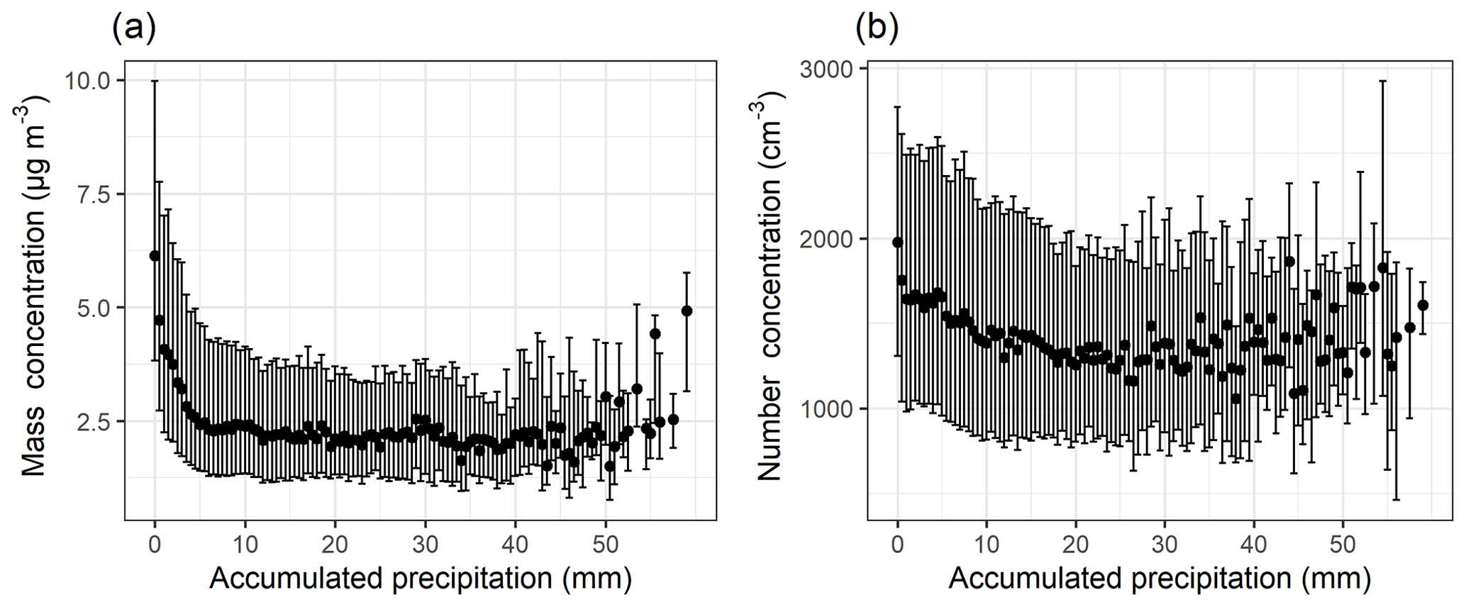
Figure 1 Total particle (d_p=3–1000 nm) mass (a) and number (b) concentration as a function of 0–50 mm accumulated precipitation along the 96 h HYSPLIT air mass trajectories. The black dots show the median values, and bars highlight the 25th–75th percentiles for each 0.5 mm bin of accumulated precipitation. The figure includes DMPS data between January 2005 and August 2019.

It should be noted here that this type of approach to air mass history analysis in which the vertical trajectory position with respect to precipitating cloud is not considered does not allow us to explicitly separate the in-cloud (particles activate to cloud droplets and collide with interstitial aerosol and then precipitate) and below-cloud (falling droplets collide with particles) precipitation scavenging (see Sect. 2.2). Instead, it gives us an estimate of the overall effect of precipitation on aerosol concentrations by using the surface precipitation provided by the air mass trajectories as a proxy for the precipitation experienced by each single particle trajectory. In addition, as we investigate aerosol scavenging in a Lagrangian framework (visualised in Fig. 2) in which the temporal and spatial scales of the reanalysis data used in the trajectory calculations are much larger than dynamic cloud processes, we cannot directly probe sub-grid-scale processes, e.g. in-cloud aerosol scavenging. Lagrangian analysis demonstrates in-cloud scavenging occurring via the removal of activated aerosol particles from the atmosphere due to precipitation scavenging. However, this is the case only if the trajectory of the air parcel coincides with the conditions we define as “precipitating cloud”. When we investigate how the size distribution changes with accumulated precipitation as demonstrated in Fig. 3, some qualitative conclusions can, however, be drawn. The strong exponential decay of particle number size distribution is visible in sizes larger than 100 nm, while the changes in the size range around 10–50 nm are small or negligible. This indicates that the large particles (d_p>100 nm) are removed most efficiently with the first 10 mm of accumulated precipitation, while smaller particles remain unaffected by any amount of accumulated precipitation. Hence, the in-cloud scavenging in our investigation is greatly dependent on the activation of aerosol particles to cloud droplets, which in turn is strongly dependent on the particle size. The number concentration of particles with diameter larger than 100 nm has been widely used as a proxy for aerosol able to activate to cloud droplets. This is also the size range where we see the largest decrease in number concentrations (Fig. 3, especially Fig. 3b) as a function of accumulated precipitation. We can qualitatively explain the observed behaviour in Fig. 3 according to a simplistic view of the complex and highly dynamical process of activation. Assuming relatively constant meteorological conditions over our trajectory transport region, we can describe the precipitation cycle by the following: after the larger particles are removed through activation into cloud droplets, of which a subset will precipitate, the size of the smallest activated particles decreases in the consecutive cloud cycle because of less competition for the available supersaturation.

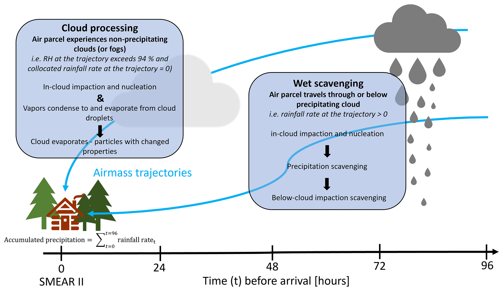
Figure 2 Schematic visualising the wet processes along air mass trajectories in the Lagrangian framework. Travelling particles experience different conditions en-route, thus alternating the observed particle concentrations (through scavenging) and composition (through cloud processing) at the SMEAR II.

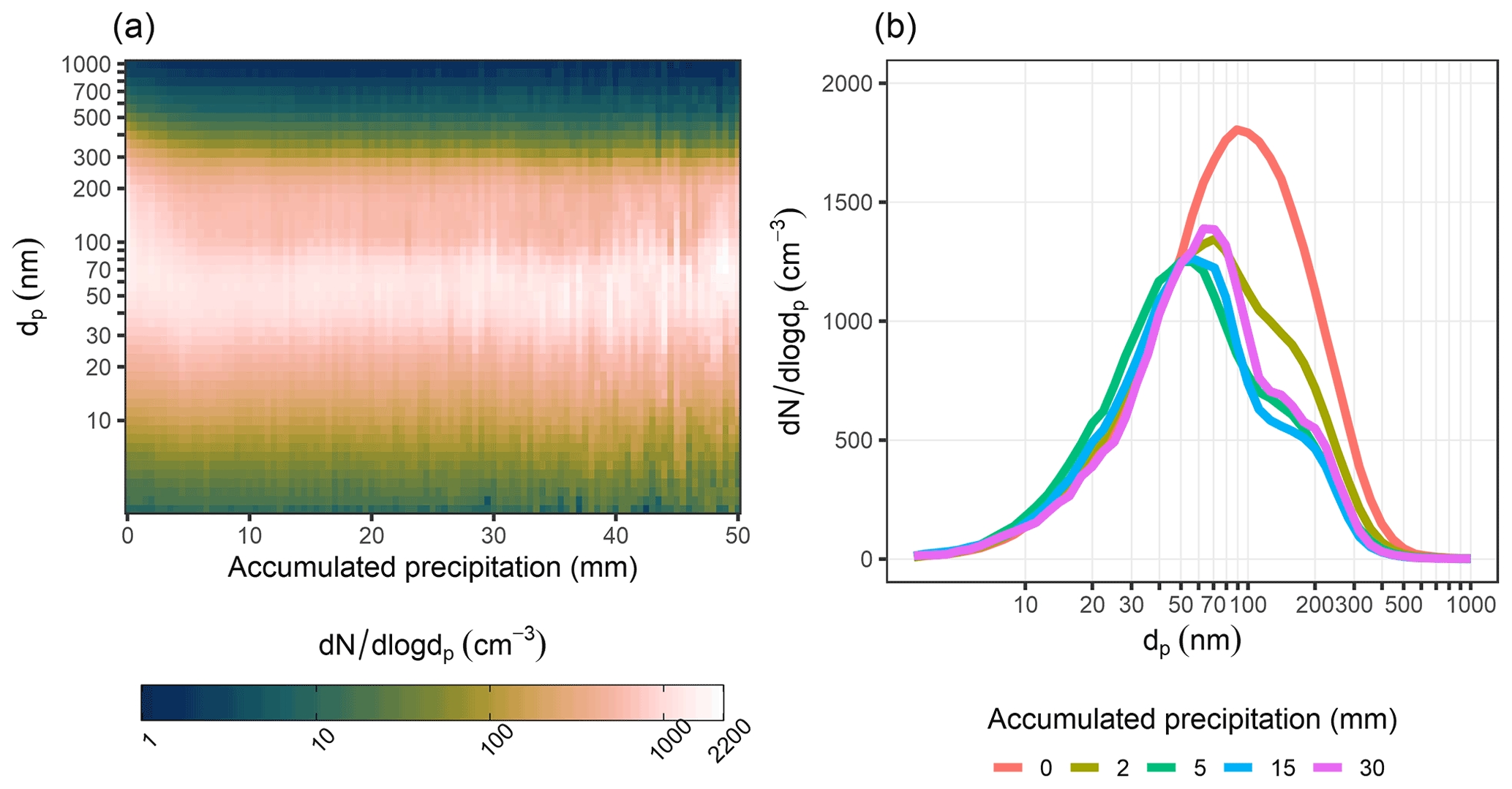
Figure 3 The aerosol size distribution (d_p= 3–1000 nm) as a function of the 0–50 mm of accumulated precipitation along 96 h air mass trajectories is shown in panel (a). Data are shown as medians for binned accumulated precipitation (bin size 0.5 mm). Median size distributions are presented for selected values of accumulated precipitation in panel (b). The figure includes DMPS data between January 2005 and August 2019.

The lowest scavenging efficiency values for below-cloud scavenging are typically in the size range of some hundreds of nanometres in diameter depending on the precipitation type (e.g. Wang et al., 2010). However, at a size range below 100 nm, the scavenging efficiency increases strongly with decreasing particle size so that at 10 nm size range, it is significantly higher. Hence, if the below-cloud scavenging would play a major role at the sub-micron size range considered here, we should see a decrease in the number concentration with accumulated precipitation in the smallest particle sizes where the below-cloud scavenging efficiencies are the highest. As shown in Fig. 3, the aerosol concentrations in the size range of 10–50 nm show no clear sensitivity (decrease) to accumulated precipitation, and the largest decreases in concentrations are shown in the size range of d_p∼100 nm and above, suggesting that in-cloud scavenging is the dominating removal mechanism in the sub-micron particle size range in the studied environment. Inspection of selected size ranges (Fig. S8) confirms that only larger sizes start exhibiting the decrease as a function of the accumulated precipitation. This has further support from earlier studies suggesting below-cloud scavenging to be a less important scavenging mechanism than in-cloud scavenging for accumulation-mode-sized particles (e.g. Tunved et al., 2013; Wang et al., 2021). Similar changes in the size distribution can be observed when the analysis was repeated using GDAS reanalysis meteorology instead of ERA-Interim (Fig. S23).

Assuming now in-cloud scavenging to be dominating and referring back to Fig. 1, the difference in the decreasing trends between particle mass and number concentration arises likely from the fact that the aerosol mass is dominated by large (d_p>100 nm) particles, which are more efficiently removed by in-cloud wet scavenging when compared to particles with smaller sizes. The aerosol number concentration, however, is dominated by particles with d_p<100 nm which are not activated to cloud droplets as efficiently as particles with larger sizes and thus not removed when the cloud precipitates. Hence the in-cloud scavenging affects the removal much less when the total particle number is inspected than in the case of large particles dominating the mass loading.

3.2 Effect of wet scavenging on the aerosol composition

The effect of accumulated precipitation on the different chemical components (organics, sulfate, black carbon, nitrate, ammonium, and chloride, hereafter Org, SO₄, eBC, NO₃, NH₄, and Chl, respectively) can be investigated using the long-term observational data (see Sect. 2.1 for details). In this study, our focus is on SO₄, Org, and eBC, and the other chemical species obtained with ACSM are included in the Supplement, as their mass concentrations are generally relatively low at SMEAR II (Heikkinen et al., 2020). To investigate possible seasonal differences in the wet scavenging of the particles, we divided the data based on monthly median temperatures (T_m). Months which have T_m<10 ^∘C (calculated from data between 2005 and 2019) include January, February, March, April, October, November, and December and are hereafter referred to as “cold” months. Months that have T_m>10 ^∘C include May, June, July, August, and September and are referred to as “warm” months. This division into two seasons is used to ensure enough data points for each bin, as the chemical composition measurements are more limited than the particle number size distributions. Each of the studied chemical components shows an exponential decrease as a function of accumulated precipitation (Fig. 4a–c), and similar decreases are also seen if the reanalysis data are changed (Fig. S24a–c).

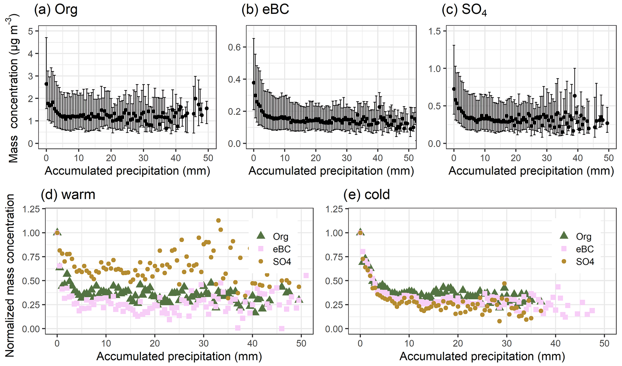
Figure 4 Particle mass concentration of (a) Org, (b) eBC, and (c) SO₄ as a function of accumulated precipitation along the 96 h HYSPLIT air mass trajectories from all seasons. The black dots in the top row show the median values, and bars highlight the 25th–75th percentiles for each 0.5 mm bin of accumulated precipitation. Panels (d) and (e) show normalised particle masses (calculated from the medians) with temperature separation. Medians and normalised medians are shown for each bin having 10 or more data points. The figure includes data between 2006–2019 for eBC and 2012–2019 for Org and SO₄.

To investigate the possible differences in the removal efficiency for different species, we normalised the median mass concentration values with the median mass concentration value when the accumulated precipitation is zero (Fig. 4d and e). The median mass concentrations (and 25th–75th percentiles) for non-precipitating trajectories for Org, eBC, and SO₄ were 3.77 (2.18–5.49), 0.28 (0.17–0.45), and 0.52 (0.34–0.88) µg m⁻³ for warm months and 2.03 (1.22–3.37), 0.48 (0.26–0.85), and 1.01 (0.51–1.53) µg m⁻³ for cold months, respectively. Org mass concentration, for example, is much higher during warm months due to strong local biogenic activity, whereas SO₄ mass concentration in warm months is ∼50 % of that in cold months, suggesting the two seasons introduced here capture the typical seasonal characteristics in this region reasonably well.

SO₄ seems to be removed less efficiently than Org and eBC during warmer months during the arrival of the air masses at SMEAR II, as can be seen from Fig. 4d. During the first 10 mm of accumulated precipitation, the normalised particle mass has decreases from 1 to 0.62 for SO₄, whereas Org and eBC have reached 0.37 and 0.32, respectively. This is surprising as sulfate is more hygroscopic than Org and eBC. There are two possible explanations for the observed differences. First, this could indicate that more of the SO₄, compared to Org and eBC, is distributed to smaller particles during warmer months. This reduces both cloud condensation nuclei (CCN) activation potential and removal of activated particles by rainfall. Second, the stronger contribution of local sources of SO₄ during warm months could distort our analysis and result in lower derived removal efficiency.

Conversely, during the colder months (Fig. 4e), SO₄ is removed slightly more efficiently than Org and BC (decreases from 1 to 0.39, 0.34, and 0.28 for Org, eBC, and SO₄, respectively, with the first 10 mm of accumulated precipitation). The differences of the removal efficiency between the investigated components are smaller during colder months when compared to warmer months, suggesting the species are internally mixed during colder months (as SO₄ and eBC, for example, have very different hygroscopicity but still are removed almost as efficiently). The trajectories derived with the GDAS meteorology precipitate, on average, less (Fig. S21) than those derived with the ERA-Interim meteorology (Fig. S1). This explains the less efficient derived removal of the standardised particle masses in Fig. S24d and e. It is also possible that the seasonal differences in cloud types and cloud cover fractions within one grid box in the reanalysis dataset could have an effect on the observed differences between the wet scavenging efficiencies.

Comparing Fig. 4d and e, we see that the data points are much more scattered during the warmer months for all three species. This could indicate a larger contribution from local production, and thus we can observe relatively large mass concentrations in SMEAR II even with high accumulated precipitation values along the air mass route. Based on the mixed effects model, the relative contribution of wet scavenging is 5–10 times smaller during the warmer months (Tables S7–S9), which show less defined removal by accumulated precipitation compared to warmer months. Regression coefficients indicate more efficient removal during colder months for all species (Tables S10–S12). Figure S9 shows the particle number size distribution for d_p=50–700 nm (electrical mobility diameter), roughly representative for the sizes measured by ACSM (ca. 75–1000 nm in vacuum aerodynamic diameter) as a function of the accumulated precipitation (like Fig. 3a) for the two temperature regimes. We clearly observe a relatively high number of particles, especially smaller ones, during warmer months despite the high values of accumulated precipitation along the trajectory. The decreases seen in the number size distribution for the different particle sizes during the first 10 mm of precipitation are steeper during the colder months. Similar behaviour (steeper decrease during colder months) is observed for SO₄ mass concentration in Fig. 4e. Based on the statistical modelling, the contribution of local meteorology to the organic mass concentration, for example, is an order of magnitude larger during warmer months (group 3 in Table S7). For SO₄ and eBC, a large difference between the seasons is seen in terms of long-range transport (group 5 in Tables S8 and S9). Long-range transport has a relatively small contribution (Sect. S3.2) in the mixed effects models during the warm months compared to colder months (i.e. the variable group is less crucial for the model with data from warmer months), and as the wet scavenging discussed here takes place along the air mass route, defined removal is not observed (as seen in Fig. 4d). Conversely, during cold months the relative contribution of long-range transport (and wet scavenging, group 4a) for SO₂ is much larger, and thus we see more defined removal (i.e. less scattering of the data points) during the colder months in Fig. 4e for eBC and SO₄.

3.3 Effect of in-cloud processing on aerosol concentrations and composition

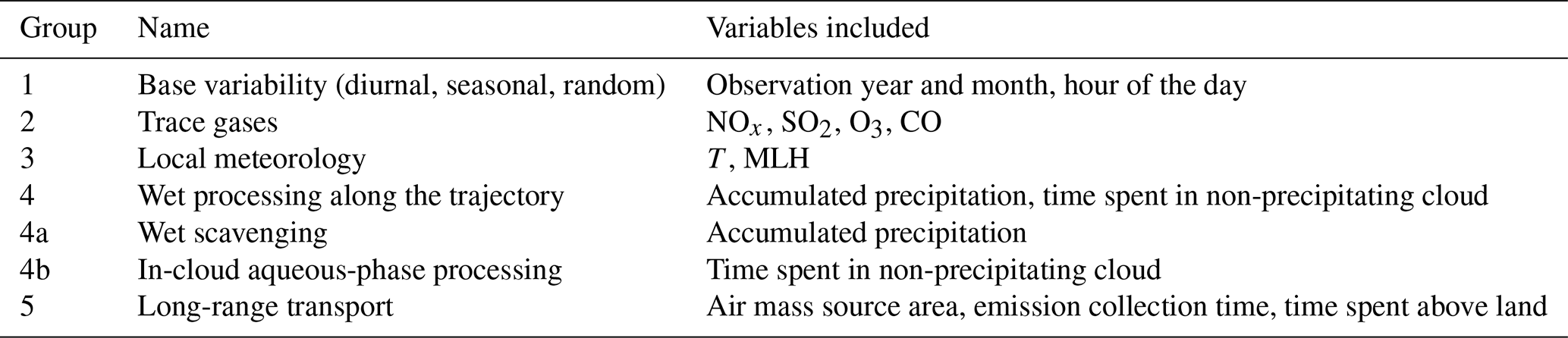
To investigate the possible effects of in-cloud processing on aerosol composition, we took advantage of the relative humidity (RH) provided by the HYSPLIT model along the air mass trajectories as described in Sect. 2.2. The observations were divided into three groups based on the conditions (precipitation and clouds) the arriving air masses have experienced during the last 24 h to investigate if precipitation and in-cloud aqueous-phase processing affect the particles differently. Group 1 represents the cases in which the arriving air masses have not experienced precipitation or clouds (i.e. RH<94 %) within the last 24 h before arriving at SMEAR II. Group 2 represents cases in which air masses have experienced precipitation within the last 24 h. Group 3 represents cases in which the air mass has experienced RH>94 % (i.e. in-cloud conditions) but no precipitation within the last 24 h. These definitions are summarised in Table 1. We restrict trajectories to the 24 h prior to arrival to ensure enough observations corresponding to the trajectories in each group, especially in group 3 which has the strictest criteria. With longer trajectories, more of the trajectories would contain precipitating clouds, which would lead to a reduction of observations in group 3. Sensitivity analysis was conducted by limiting air mass experience to 36 and 48 h, but the same conclusions were achieved.

Table 1 Definitions for the wet processing groups. Availability shows the percentage of trajectories relative to total number of trajectories belonging to the wet processing groups. Definitions are according to description of explained quantities in Sect. 2.2.

Figure 5 shows the median mass (a) and number (b) concentration of the accumulation mode (d_p=100–1000 nm) particles based on their experiences of precipitation and high-humidity conditions (RH>94 %) during the last day before arrival at SMEAR II, as described in Table 1. The Mann–Whitney U test (Mann and Whitney, 1947) was applied to assess the statistical significance of the differences between the groups. Figure 5b shows that the accumulation mode number concentration is lower if the air mass has experienced precipitation (group 2) or high-humidity conditions (i.e. clouds) without precipitation (group 3), compared to the case when the air mass has not experienced precipitation or in-cloud conditions (group 1). When the mass concentration (Fig. 5a) is investigated, we see higher mass concentration for group 3 compared to group 1, suggesting that in non-precipitating, high-RH conditions the aerosol mass increases due to aqueous-phase processes. The observed differences between the wet processing groups for both mass and number concentration were statistically significant (Table S4). Identical observations can be made if the GDAS reanalysis meteorology is used in the calculation of the trajectories (Fig. S25).

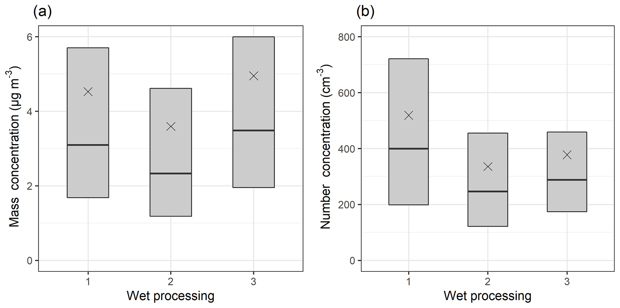
Figure 5 Median (black horizontal lines), mean (black crosses), and 25th–75th percentiles (boxes) for accumulation mode (d_p=100–1000 nm) particle mass (a) and number (b) concentration for wet processing groups described in Table 1. The figure includes DMPS data between January 2005 and August 2019.

To investigate further the observed increase in accumulation mode mass concentration (Fig. 5a) when the air mass had experienced high-humidity conditions, we investigated the bulk aerosol composition. We focus on group 1 (no wet processing at all) and group 3 (high-humidity conditions but no precipitation), as we are now interested in the increase in mass concentration between those groups, as shown in Fig. 5a. Here, we concentrate on the mass concentrations of organics (Org) and sulfate (SO₄), as well as black carbon (eBC) measurement data. Figure 6 shows the median particle mass concentrations (see Fig. S10 for mass fractions) for each of these chemical species for clean and more polluted air masses with the temperature division for the wet processing groups 1 and 3. The division of the trajectories into “clean” and “polluted” sectors was made by assigning any trajectories that visited latitudes below 60^∘ north into the polluted sector and the rest to the clean. Thus, our final subgroups are WC (warm, clean), WP (warm, polluted), CC (cold, clean), and CP (cold, polluted). This approach was applied to make sure the observed changes in the concentration of species are indeed related to the aqueous-phase processing and to exclude the influence of artefacts arising from the possible association of different source areas to different meteorological conditions (i.e. group 1 vs. group 3). This type of source area artefact could take place, for example, if cloud occurrence would be more frequent for air masses arriving from certain directions, which could (randomly) coincide with higher SO₄ observations. Further justification for our choice of these sectors can be found in the chapter below. Statistically significant (Table S5) increases (except subgroup WC, which shows a small decrease) in SO₄ concentration (Fig. 6) are observed between wet processing groups 1 and 3, suggesting SO₄ formation in the aqueous phase, while no significant changes are observed for Org. Black carbon shows both increases and decreases in mass, depending on the subgroup. The patterns in the mass concentrations for each species between the groups 1 and 3 showed similar behaviour when we increase the time (0–24 h into, for example, 0–36 or 0–48 h) used to determine the classes.

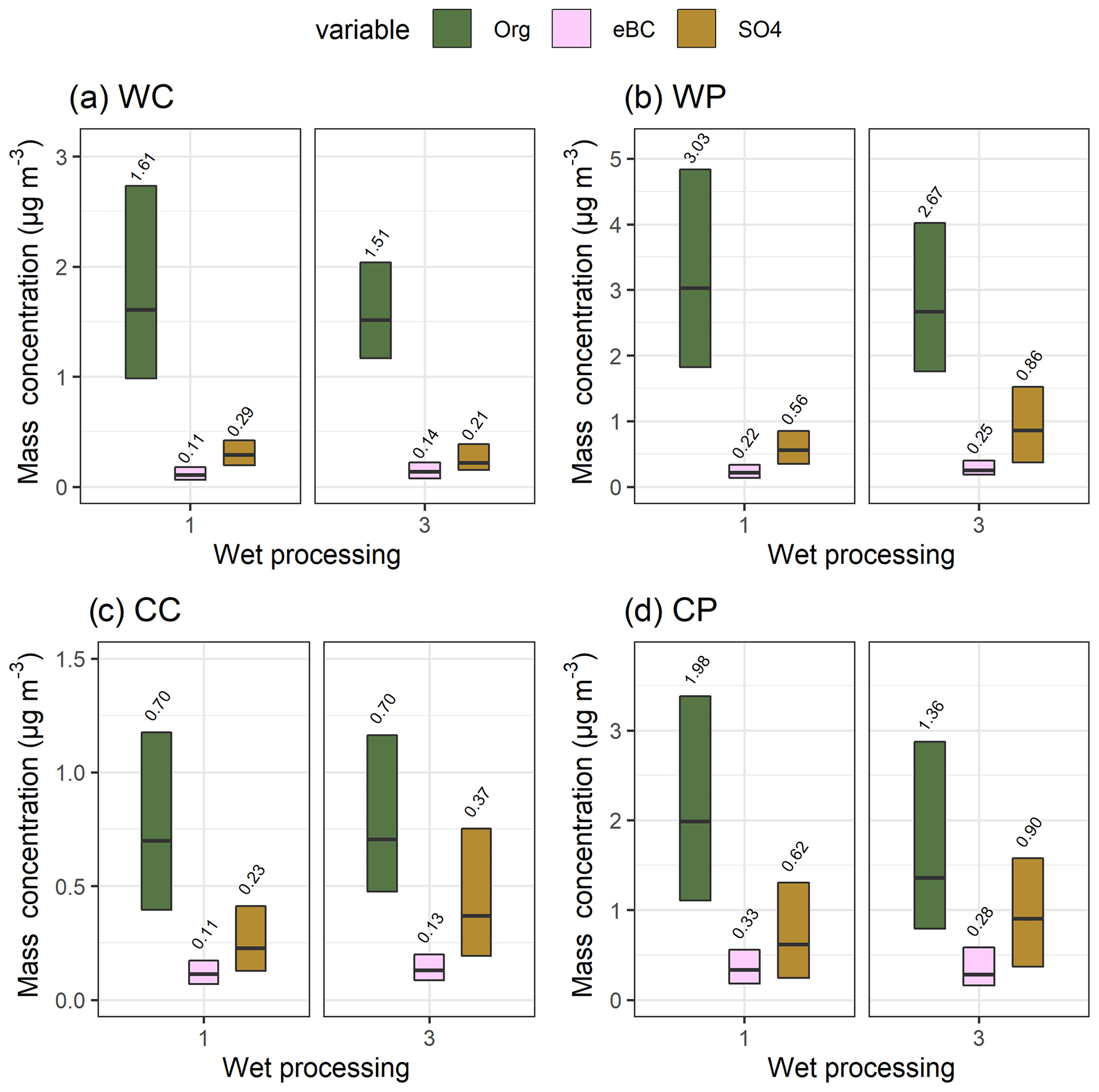
Figure 6 Median (black horizontal lines and numerical values) particle mass concentration with 25th–75th percentiles (boxes) for Org, eBC, and SO₄ for wet processing groups 1 and 3 as described in Table 1. Subplots show the air mass sectors (clean and polluted) with the seasonal (warm and cold) division: (a) warm and clean, (b) warm and polluted, (c) cold and clean, and (d) cold and polluted. The figure is based on simultaneous observations of these three species between March 2012 and August 2019. Note the different y-axis limits in each subplot.

Two sectors were used to distinguish the more polluted and mostly clean air masses, as more detailed division on air mass source areas is not possible because of the limited amount of data available especially for the group 3 cases. Even though the division is relatively rough, it does separate the air masses quite well, especially as we have already excluded the highly polluted air masses arriving from the Kola Peninsula and emissions arriving from the nearby sawmills. For example, in a former study from Kulmala et al. (2000), trajectories arriving from the Arctic ocean coincide with a low number of accumulation mode particles and low SO₂ concentration, and, therefore, air masses arriving from that sector are classified as “clean”. Sogacheva et al. (2005) also presented similar sources for accumulation mode particles. The same classification is used in this study. Sectors from Kulmala et al. (2000) including the southeast of Russia and central Europe showed the highest accumulation mode number and SO₂ concentrations and are classified as “polluted” also in our study. We selected two sectors to maintain statistics that are high enough for the composition measurements to achieve reliable results. In addition, the temperature-based division, discussed in Sect. 3.1, gives additional insight when separating the air masses. Riuttanen et al. (2013), conducted trajectory analysis to investigate trace gases observed in SMEAR II, and our temperature-based division coincides well with the seasonality of SO₂ concentration. They concluded, for example, that combustion-related SO₂ is mainly transported to SMEAR II from eastern Europe during winter months. In addition, for high particle concentrations arriving at SMEAR II, they observed the air mass origins to be dependent on particle size.

To further confirm that the seasonal patterns of trace gases like SO₂ and aerosols shown in Riuttanen et al. (2013) also hold for our study period, source contribution analysis was conducted. No major changes in the source areas are observed (Figs. S17 and S18 as examples for accumulation mode particle number concentration and SO₂ mixing ratio, respectively) when compared to the study from Riuttanen et al. (2013). We can observe a clear difference in the total mass concentration between clean and more polluted air masses in Fig. 6, indicating our sector division into mainly clean and more polluted is suitable. The average particle number size distribution with these sector- and temperature-based divisions is shown in Fig. S11, but the reader should be aware that the composition measurements do not represent particles with d_p<70 nm. There is no clear difference in the geographical distribution of air mass trajectories between the wet processing groups 1 and 3 shown in Fig. 7; thus we can conclude that the observed differences in SO₄ are not associated with different source areas of air masses between the groups 1 and 3. Group 3 includes fewer trajectories due to our strict definitions of the air mass history groups, but the trajectories are arriving from similar areas in both group 1 and group 3. Further, to show that the increase in sulfate concentrations is driven by sulfate formed mostly in the clouds and not just directly above the sea surface derived, for example, from dimethyl sulfide emissions (e.g. Barnes et al., 2006), we investigated the vertical transport of the air masses. This analysis showed no evidence (see Sect. S4) that this type of transport is significantly influencing the results presented here.

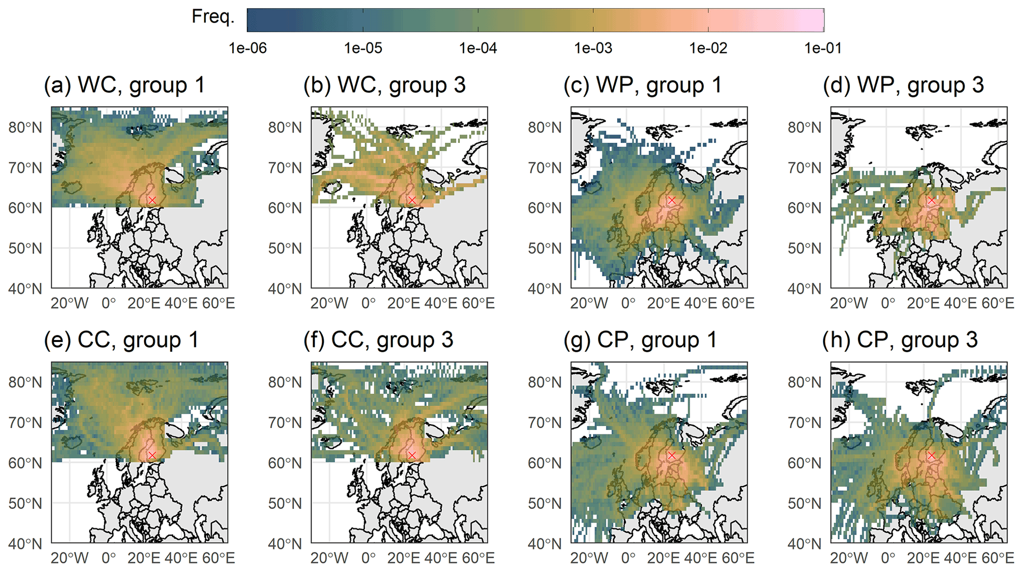
Figure 7 The 96 h air mass history for the wet processing groups (1 and 3) with the sector (clean and polluted) and temperature (warm and cold) division. Subplots show (a, b) warm and clean, (c, d) warm and polluted, (e, f) cold and clean, and (g, h) cold and polluted. Colour scale shows the frequency (crossings in each $\mathrm{1}{}^{\circ }\times \mathrm{1}{}^{\circ }$ grid point divided by total number of crossings in each group) of trajectories crossing a grid point. The groups 1 and 3 correspond to the air mass history groups presented in Table 1. The red cross shows the location of SMEAR II.

Thus, based on the air mass history analysis presented above and conclusions drawn regarding SO₄ transport from oceans, we can state that the observed increase in SO₄ is likely due to aqueous-phase chemistry, in which SO₂ is oxidised in the aqueous phase to form SO₄ (e.g. Barth et al., 2000; Ervens, 2015; McVay and Ervens, 2017). A relative increase of 45 %–63 % is observed between groups 1 and 3 in Fig. 6b–d (air mass histories WP, CC, CP), and the largest increase is observed for more polluted air masses during colder months (CP). The increase in SO₄ concentration is not seen for clean air masses during the warmer months (Fig. 6a, WP), as, for example, SO₂ concentration, an important precursor for in-cloud SO₄ formation, is lower in cases for air masses coming from northern areas and for the warm season (Kulmala et al., 2000; Riuttanen et al., 2013). For the colder months and more polluted air masses (Fig. 6b–d), the increase in SO₄ is more pronounced due to more precursor SO₂ available for in-cloud SO₄ production (e.g. Paulot et al., 2017). The increasing trends in SO₄ mass concentration and mass fraction are similar to what is shown in Fig. 6, when all chemical species measured by the ACSM are considered (mass concentrations in Fig. S12, mass fractions in Fig. S13). In addition, small increases in the mass concentration of NH₄ can be observed for group 3. This is likely because of the enhanced uptake of ammonia from the gas phase with increasing sulfate fraction (Harris et al., 2014). Changes in the SO₄ concentration due to aqueous-phase processing are similar also when the GDAS reanalysis meteorology is used. In-cloud formation of SO₄ is also supported by the statistical model in which we consider the other factors also affecting the local particle concentrations (Table S11).

The median mass concentration of Org shows a decrease when comparing group 1 to group 3 in Fig. 6a, b, and d but no change in the cold and clean subgroup (Fig. 6c, CC). However, the observed decreases were not statistically significant (Table S5) at the α=0.01 limit. With trajectories using GDAS reanalysis meteorology, decreases in the median mass are also observed for the same subgroups. Previous studies have shown an increase in organic mass through aqueous-phase production of SOA (Blando and Turpin, 2000; Ervens and Volkamer, 2010; Ervens et al., 2018). For example, Ervens et al. (2018) investigated the formation of aqSOA with parcel models from gas-phase precursors of toluene, xylene, and ethylene. In SMEAR II, the gas-phase precursors from biogenic sources are dominated by monoterpenes especially during warm months (e.g. Hakola et al., 2012; Patokoski et al., 2015; Barreira et al., 2017; Heikkinen et al., 2021).

During the colder months (Fig. 6c and d), the air masses are likely to have more anthropogenic influences and thus a different VOC profile (e.g. Patokoski et al., 2015), but the formation of aqSOA is still negligible when the total Org mass is investigated in this area of northern Europe. It has also been suggested that water soluble SOA (originating from other sources than aqueous-phase processing) in the cloud droplets can become oxidised to form more volatile compounds leading to evaporation. This could lead to a decrease in total SOA mass, even though additional aqueous-phase SOA mass is formed (Ervens et al., 2018). In addition, the increase in SO₄ can increase the acidity of the droplets which might increase the evaporation of organic acids leading to a decrease in the organic mass (Ervens et al., 2018). Our data suggest that the local photochemically driven SOA production at SMEAR II (and surrounding areas) dominates over the aqueous-phase SOA formation especially during the warm months. This is supported by the solar radiation values measured at SMEAR II (not shown), as they are much lower for group 3 than for group 1 for all cases. Hence, decreased SOA formation due to the decreased photochemical activity could compensate for the in-cloud aqueous-phase SOA formation resulting in comparable total organic mass when groups 1 and 3 are compared. Our results indicate that in the boreal-forest-dominated northern Europe the photochemical SOA formation in the gas phase dominates over SOA formation in the aqueous phase, when the total organic mass is considered. This applies for both warmer and colder seasons, as well as in the case of clean and polluted air masses. The Org mass concentration also shows no increase due to clouds when the other factors affecting the local concentrations are considered with the mixed effects model (Table S10).

Figure 8 The mass fractions of Org, SO₄, and eBC for clean and more polluted air masses as a function of time spent in RH>94 % (a, c) and in precipitation (b, d). The figure shows median values for each 1 h bin, if 10 or more data points were available in the bin. The figure is based on observations between March 2012 and August 2019.

When investigating the composition of the particles as a function of time in RH>94 % (Fig. 8) when no distinction relative to precipitation is applied (i.e. time in-cloud can also include precipitating clouds), we observe an increase in sulfate mass fraction with time spent under the high-humidity conditions. This is most clear for the more polluted air masses which also have more SO₂ available for the in-cloud production of SO₄ (Fig. 8a). This trend is not seen when looking at the time the air mass was influenced by precipitation (Fig. 8b), indicating precipitation acts mainly as a sink for the particles, whereas high-humidity conditions, i.e. in-cloud aqueous-phase processing, also alter the particle chemical composition. Inspection of the absolute mass of the species (Fig. S14) also shows an increase in SO₄ mass with longer exposure times in RH>94 %, whereas decreases in mass of all species is seen with increasing time of experienced precipitation. The increasing trend in SO₄ fraction when the air masses arrive from cleaner areas is more subtle (Fig. 8c). The same trends are observed when all species from the composition measurements are investigated (Fig. S15). These results suggest that not only the experience of in-cloud aqueous-phase processing (Fig. 6) affects the particle composition but also the time spent in cloud has an effect. Unfortunately, with this type of analysis of the time dimension, we were not able to apply the temperature-based division in addition to the sector division, as it would limit the number of observations for the long exposure times too much to obtain statistically reliable results. Results obtained with the GDAS reanalysis meteorology (Fig. S28) agree well with those from Fig. 8. The very long exposure times (>60 h) of precipitation are missing from the GDAS-derived trajectories due to lower occurrence of precipitation events compared to the ERA-Interim-derived trajectories (see Figs. S1 and S21).

To investigate which particle sizes are most affected by the increasing mass of SO₄, the DMPS size distribution was divided into seven classes with particle dry diameter ranges (in nm) of [3,30], (30,50], (50,100], (100,200], (200,350], (350,600], and (600,1000]. Using the air mass history groups presented in Table 1, the mass concentrations for these size classes are shown in Fig. 9 corresponding to the sector and temperature divisions first shown in Fig. 6. The mass concentration is larger if the air mass has experienced high-humidity conditions (group 3) for particles with diameters between 200 and 1000 nm when compared to group 1 for which there have not been any wet processes in the last 24 h. The same observation can be made with the trajectories using GDAS meteorology (Fig. S29). The increase is clearest in the size ranges (200,350] and (350,600], and the size range (600,1000] shows a very minor increase in mass for some subgroups. The changes in mass are also statistically significant except for sector CP for size ranges (200,350] and (600,1000] (Table S6). The same changes are also seen when the particle mass data are strictly limited to simultaneous observations with the composition (Org, SO₄, BC) measurements (Fig. S16). These results suggest that the SO₄ formed via in-cloud aqueous-phase processes is mainly distributed to particles having a dry diameter between 200 and 1000 nm.

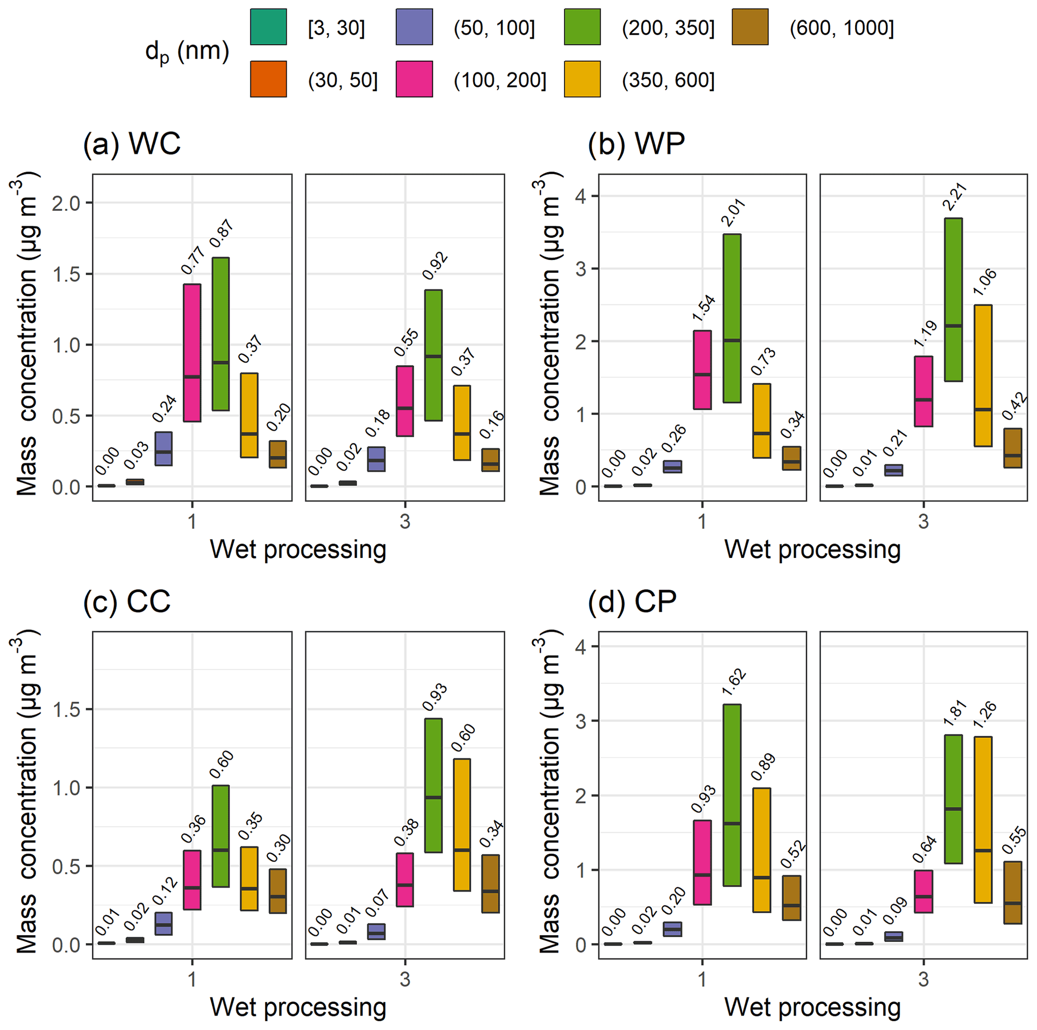
Figure 9 Median (black horizontal lines and numerical values) particle mass concentration with 25th–75th percentiles (boxes) for size bins derived from the DMPS measurements for wet processing groups 1 and 3 as described in Table 1. Subplots show the air mass sectors (clean and polluted) with the seasonal (warm and cold) division: (a) warm and clean, (b) warm and polluted, (c) cold and clean, and (b) cold and polluted. The figure includes all available data between January 2005 and August 2019. Note the different y-axis scale in each subplot.

4 Conclusions

In this study, we investigated wet processes in clouds including aerosol wet scavenging and aqueous-phase oxidation along air mass trajectories. We examined how they affect the observed sub-micron aerosol population in SMEAR II station, which represents the boreal environment.

Our first objective was to investigate how efficiently different chemical species are removed from the atmosphere by precipitation. We observed, based on a time series over a decade long, an exponential decrease in particle mass as a function of accumulated precipitation along the trajectory, similar to that reported in earlier studies. We concluded that in-cloud wet scavenging dominated over below-cloud precipitation scavenging, especially for particles of accumulation-mode size ($\mathrm{100}\mathrm{nm}<d_{\mathrm{p}}<\mathrm{1}$ µm). Particle mass scavenging was more effective during colder months especially for sulfate aerosol, whereas the behaviour of other aerosol chemical species investigated was more alike. Statistical mixed effects models also exhibited removal by accumulated precipitation for all species, suggesting more efficient removal in colder months. In addition, scavenging efficiencies were relatively similar between species in colder months, suggesting that particles were internally mixed, and different species were distributed to similar-sized particles. During warmer months, strong local particle production at SMEAR II likely effectively masks wet scavenging along the trajectory. Thus, despite high values of accumulated precipitation, relatively high particle mass concentrations exist. This finding was supported by statistical modelling, wherein, for example, the relative contribution of local meteorology to organic aerosol production was much larger during warmer months. Seasonal differences in cloud types and cloud cover fractions within one grid box in the reanalysis dataset may also influence the differences observed between seasons in wet scavenging efficiencies.

Our second objective was to investigate how aqueous-phase processing occurring in clouds alters particle mass concentration and composition. Our study revealed a significant in-cloud formation of sulfate mass, but aqueous-phase SOA formation could not be identified by the analysis. In-cloud processing was separated by using relative humidity as a proxy for air mass with cloud experience. The precipitation data along the air masses were used to separate non-precipitating clouds. An increase in accumulation mode particle mass was observed for air masses that had recently been in-cloud when compared to clear sky air masses which had no experience of clouds or rain during the last 24 h. In the chemical composition of accumulation mode particles, the increase observed in particle mass can be mostly attributed to in-cloud SO₄ production. Our analysis showed that, due to in-cloud sulfate formation, sulfate mass concentrations increased 45 %–63 %, depending on season and air mass origin. Furthermore, the increase in sulfate mass fraction was higher when the air mass had spent more time in high-humidity conditions. We considered, in the statistical mixed effects model, additional factors affecting local SO₄ concentrations. This model also supported in-cloud SO₄ formation, whereas no formation of Org or eBC mass was observed.

Air mass history analysis was applied to separate air masses originating from different sources (more polluted and mostly clean) in addition to temperature-based seasonal division. Thus, we investigated how different conditions along the air mass trajectories affected the increase observed in SO₄ mass concentration due to in-cloud processes. When air masses originated from areas with more pollution sources producing gaseous SO₂, we observed a greater increase in SO₄ mass. This increase was due to more SO₂ being available in the gas phase to be oxidised in-cloud to form SO₄. Increases in the total organic mass due to aqueous-phase processing was not observed. We were also interested whether the effects of aqueous-phase processes were different for particles of different size. Therefore, we investigated changes in particle number size distribution to determine into which particle sizes the mass increase observed in SO₄ was mostly distributed. Increases in particle mass occurred for sizes larger than 200 nm, whereas smaller sizes displayed a decrease in some cases.

Finally, as an additional robustness test for our results, we also compared the trajectories based on different reanalysis meteorologies, ERA-Interim and GDAS. Both approaches yielded nearly identical results, supporting the same conclusions. Trajectories obtained with GDAS reanalysis meteorology had, in general, fewer precipitation events. Thus, compared to that in ERA-Interim-based trajectory results, the scavenging efficiency of the species investigated was lower. With both approached, aqueous-phase SO₄ formation significantly contributed to the total SO₄ mass, whereas aqSOA formation was undetected. Precipitation values derived from the trajectory model at SMEAR II agreed well with locally measured precipitation. The results from this study offer interesting insights into using air mass history analysis to study aerosol–cloud interactions. These findings facilitate the comparison of observed aerosol wet scavenging and in-cloud processing with outcomes of larger-scale models. Global models can simulate aerosol composition and size distribution, especially away from source regions. This study highlights that this ability can be enhanced by improving the description of size-dependent wet removal of different aerosol compounds. Our analysis also provides a good platform for evaluating the ability of models to simulate in-cloud chemical formation of aerosol. Regarding the effect of clouds and precipitation on aerosol dynamics and detailed changes in size distributions, further, in-depth investigations are imperative.

Appendix A

The formulation of the final fitted equation can be expressed as

$$\begin{array}{}\text{(A1)}& \begin{array}{rl}& \left[{\text{VAR}}_i\right]\\ & ={\mathit{\beta }}_{\mathrm{0}}+\left\{{\mathit{b}}_{\text{h}}+{\mathit{b}}_{\text{m}}+{\mathit{b}}_{\text{y}}\right\}\\ & +\left\{{\mathit{\beta }}_{\mathrm{1}}\left[\mathrm{NO}{x}_i\right]+{\mathit{\beta }}_{\mathrm{2}}\left[{\mathrm{SO}}_{\mathrm{2},i}\right]+{\mathit{\beta }}_{\mathrm{3}}\left[{\mathrm{O}}_{\mathrm{3},i}\right]+{\mathit{\beta }}_{\mathrm{4}}\left[{\mathrm{CO}}_i\right]\right\}\\ & +\left\{{\mathit{\beta }}_{\mathrm{5}}{T}_i+{\mathit{\beta }}_{\mathrm{6}}\left[{\text{MLH}}_i\right]\right\}\\ & +\left\{\exp \left({\mathit{\beta }}_{\mathrm{7}}{\text{accum.precip}}_i\right)+{\mathit{\beta }}_{\mathrm{8}}{\text{time.in.cloud}}_i\right\}\\ & +\left\{{\mathit{\beta }}_{\mathrm{9}}{\text{emission.col.time}}_i+{\mathit{\beta }}_{\mathrm{10}}{\text{time.in.land}}_i+{\mathit{b}}_{\text{a}}\right\},\end{array}\end{array}$$

where [VAR] is now the mass concentration of either Org, SO₄, or eBC, β₀ is a model intercept, b_h, b_m, b_y, and b_a are the vectors of random intercepts for hour of the day, month, year, and air mass source area, respectively, and β₁–β₁₀ are the fixed regression coefficients. Subscript i denotes the time point, i.e. one observation. Thus the predictor variables (see Sect. 2.1 for the abbreviations) include concentrations of SO₂, CO, NO_x, and O₃ (trace gases), air T and MLH (at SMEAR II derived from the back-trajectory data) describing the local meteorology, and the following trajectory-derived variables: accumulated precipitation along the trajectory (mm), time spent in high-humidity conditions without simultaneous rain (“in non-precipitating cloud”, h), emission collection time (time in mixed layer until rain event, h), and total time the air mass has spent over land (h). In addition, the air mass source areas (obtained by clustering as explained in Sect. 2.2 and visualised in Figs. S3 and S4) and observation year, month, and hour of the day were included, as shown in Eq. (A1). A summary of the used predictor variables in the regression is shown in Table A1, and each predictor variable group is separated with curly brackets in Eq. (A1). The process leading to the selection of the response variables is explained in detail the Sect. S3.1.

Table A1 Predictor variables used in regression.