the Creative Commons Attribution 4.0 License.
the Creative Commons Attribution 4.0 License.
 | 09 Sep 2022
Attribution of surface ozone to NOx and volatile organic compound sources during two different high ozone events
Aurelia Lupaşcu
Noelia Otero
Andrea Minkos
Tim Butler
Increased tropospheric ozone (O3) and high temperatures affect human health during heat waves. Here, we perform a source attribution that considers separately the formation of German surface ozone from emitted NOx and volatile organic compound (VOC) precursors during two peak ozone events that took place in 2015 and 2018 which were associated with elevated temperatures. Results showed that peak ozone concentrations can be primarily attributed to nearby emissions of anthropogenic NOx (from Germany and immediately neighboring countries) and biogenic VOC. Outside of these high ozone episodes, baseline ozone concentrations are attributed primarily to long-range transport, with ozone due to remote anthropogenic NOx emissions and methane oxidation adding to the tropospheric ozone background. We show that a significant contribution to modeled O3 coming from German NOx or VOC emissions occurs mostly in southern Germany, emphasizing that the production of ozone depends on the local interplay between NOx and VOC precursors. Shipping activities in the Baltic and North seas have a large impact on ozone predicted in coastal areas, yet a small amount of ozone from these sources can also be seen far inland, showing the importance of transported ozone on pollution levels. We have also shown that changes in circulation patterns during the peak O3 episodes observed in Germany during the 2015 and 2018 heat waves can affect the contribution of different NOx emission sources to total O3; thus, the possible influence of multiple upwind source regions should be accounted for when mitigation strategies are designed. Our study also highlights the good correlation between ozone coming from German biogenic VOC emissions and total ozone, although the diurnal variation in the ozone coming from biogenic sources is not dominated by the diurnal variation in biogenic emissions, and the peaks of ozone from biogenic sources are disconnected from local emission peaks. This suggests that the formation of O3 from local German biogenic VOC emissions is not the sole factor that influences the ozone formation, and other meteorological and chemical processes affect the diel variation of ozone with a biogenic origin. Overall, this study helps to demonstrate the importance of a source attribution method to understand the sources of O3 in Germany and can be a useful tool that will help to design effective mitigation strategies.
- Article
(10687 KB) - Full-text XML
-
Supplement
(3007 KB) - BibTeX
- EndNote


Increased concentrations of ground-level ozone can harm humans and vegetation, especially during hot summer days (Sillmann et al., 2021). As shown by Analitis et al. (2014), the heat wave effect combined with the high ozone episodes is associated with an increase in mortality. Recent Intergovernmental Panel on Climate Change (IPCC) assessment reports (IPCC, 2012; Smith, et al., 2014) associate an increase in the occurrence of extreme heat wave episodes with an increase in socioeconomic costs and with an increase in ozone concentrations that cause morbidity from other diseases.
Several well-documented heat waves associated with high ozone concentrations were registered over central and western Europe, such as in August 2003 (i.e., Vautard et al., 2005; Vieno et al., 2010) and July 2006 (i.e., Struzewska and Kaminski, 2008). Vautard et al. (2005) studied the 2003 heat wave using the CHIMERE model, which reproduced the high observed ozone concentration at European monitoring stations very well. Struzewska and Kaminski (2008) have identified three independent factors that influence the level of photochemical pollution, such as the circulation patterns, the geographical location, and the intensity of anthropogenic nitrogen oxide (NOx) emissions. Many studies showed that the main meteorological factor which drives high ozone pollution episodes is the temperature (i.e., Lin et al., 2001; Jacob and Winner, 2009; Porter et al., 2015; Pusede et al., 2015, and references therein; Otero et al., 2016, and references therein). Schnell and Prather (2017) showed that extreme events of ozone and temperature over North America often overlap, although consistent offsets in space and in time are occurring, most likely due to advection of emitted precursors.
During the last few decades, global and regional chemical models were used to simulate the enhanced ozone concentrations associated with heat waves (i.e., Guerova and Jones, 2007; Ordóñez et al., 2010) and future high ozone episodes (Shen et al., 2016). Meehl et al. (2018) used a model simulation for a present-day climate and showed that, during heat wave days, the surface ozone enhancement exceeds 10 ppb (parts per billion) over Europe compared to non-heat-wave days. Chemical transport models (CTMs) are an important tool for the simulation of transport and transformation of gases and for studying the relationship between meteorology and high air pollution episodes. More recent developments of CTMs enabled their capacity to tag the emissions by source (e.g., Grewe et al., 2017; Butler et al., 2018, 2020a; Lupaşcu and Butler, 2019; Mertens et al., 2020); hence, they can help to identify the main precursor sources contributing to ozone peaks.
Several studies have quantified the contribution of long-range transport vs. the impact of local emissions on summer peak ozone in Europe. Jonson et al. (2018) showed that, for most of the models used in their intercomparison study, except for the model CHASER_re1 in summer, the contribution to European seasonal mean ozone levels is larger for regions outside Europe than the contribution from European sources. Pay et al. (2019) showed that imported ozone is the largest contributor to the ground-level high ozone concentrations registered in Spain in July 2012. Lupaşcu and Butler (2019) indicated that the local sources (precursors emitted within receptor regions) explain up to 35 % of modeled daily maximum 8 h average ozone (MDA8 O3) in several receptor regions, while the remote sources accounted for 11 % to 45 % of the total surface ozone. Their work also showed the importance of locally emitted NOx precursors for the ozone metrics that are especially influenced by high values of ozone, such as MDA8 O3, AOT40, W126, and the 95th percentile.
Methane (CH4) oxidation explains a large part of the ozone formation in the troposphere. Wang and Jacob (1998) showed that the historic increase in global methane emissions and its subsequent oxidation led, among other causes, to the increase in tropospheric ozone concentrations, but this increase depends on the local availability of OH radicals. Turnock et al. (2018, 2019) showed that the reduction in CH4 is a key factor for controlling the increase of future surface ozone. West and Fiore (2005) analyzed the advantages of low ozone due to methane emission reductions on agriculture, forest management, and human health, and they found that the monetized global benefits would justify cutting the methane emissions by ∼17 %. In addition, Fiore et al. (2008) showed that the CH4 oxidation has contributed ∼20 % to the annual mean MDA8 O3 at nearly all U.S. MDA8 O3 surface locations since the pre-industrial era, while Butler et al. (2020a) indicated that CH4 oxidation explains 35 % of their simulated global average tropospheric ozone burden.
Biogenic volatile organic compound (BVOC) emissions contribute strongly to the formation of ozone (e.g., Fiore et al., 2011; Curci et al., 2009; Qu et al., 2013; Tagaris et al., 2014; Zhang et al., 2017). Among them, isoprene is the main component. Biogenic isoprene emissions depend on multiple environmental drivers such as temperature, solar radiation, plant water stress, ozone, CO2 concentrations, and land cover. Although Simpson et al. (1995) showed that, during summertime, the BVOC emissions exceed anthropogenic emissions in many countries, Simpson (1995) performed several simulations (one in which the isoprene emissions were turned off) and concluded that the isoprene emissions do not strongly influence the long-term average simulated O3 concentrations. Using long-term measurements acquired at Ispra, Italy, Duane et al. (2002), however, showed that the contribution of locally emitted isoprene to the local ozone formation reached up to 50 %–75 % during the summer of 2000. More recent studies that are mainly using two sets of simulations, one with and one without considering biogenic emissions, assessed the importance of BVOC on O3 formation. Tagaris et al. (2014) showed that the European BVOC emissions increased the predicted MDA8 O3 by 5.7 % for July 2006. Jiang et al. (2019) have used two biogenic models, one predicting 3 times more isoprene emissions than the other, and still the BVOC emissions contribute less than 10 % of the mean O3 concentration in the summer of 2011. Churkina et al. (2017) indicate that biogenic emissions explain, on average, ∼12 % of modeled mean ozone in Berlin for two summers (June–August); yet, on hot summer days, these sources are responsible for up to 60 % of the modeled MDA8 O3 concentrations. Zhao et al. (2016) showed that the use of a newer version of the Model of Emissions of Gases and Aerosols from Nature (MEGAN) better reproduces the observed isoprene than the publicly available version of the MEGAN model integrated into WRF-Chem (Weather Research and Forecasting model coupled to chemistry), which ultimately will impact the surface O3 concentration. Moreover, Zhang et al. (2021) noted that the use of multiple versions of MEGAN has significantly influenced the ozone concentration due to the changes in simulated biogenic emissions.
One important sink for tropospheric ozone is given by ozone dry deposition, which is dominated by stomatal uptake by vegetation (Turnipseed et al., 2009; Lin et al., 2019, and references therein). Moreover, Lin et al. (2020) showed that a reduced ozone uptake by vegetation worsens the severe ozone pollution during heat wave events. When the water vapor pressure deficit is high, the plants close their stomata to prevent water loss. However, most models use the Wesely deposition scheme (Wesely, 1989), which does not account for the humidity deficit and depends solely on temperature and radiation and, consequently, overpredicts the deposition of ozone under hot and dry conditions. Rydsaa et al. (2016) compared measurements of the stomatal conductance and stomatal ozone flux acquired during three summer field campaigns at three different sites in Italy with the modeled results predicted by using the Wesely scheme embedded within WRF-Chem. It has been shown that the model underestimated nighttime stomatal ozone uptake and consequently overpredicted ozone concentration in the stable nighttime planetary boundary layer. The model also overestimated the daytime stomatal conductance, leading to underestimated midday ozone concentration, highlighting the existence of some systematic biases in the model parameterization.
In this study, we focus on the origin of elevated ozone levels observed over Germany during the periods of 6–13 August 2015 and 1–8 August 2018. The 2015 and 2018 summers have been the subject of several studies due to the severity in terms of temperature and precipitation. The summer of 2015 showed high drought conditions and was characterized by high temperatures in many parts of central and eastern Europe (Hoy et al., 2016; Ionita et al., 2017). Several heat wave episodes occurred from the end of June until September, which were linked to persistent blocking conditions and a northward deflection of Atlantic storm tracks (Ionita et al., 2017). Orth et al. (2016) showed that the 2015 summer was a concurrent dry and hot extreme in most of central Europe. Similarly, other studies have analyzed the summer of 2018 in central Europe, which was characterized by extremely dry and hot conditions (Buras et al., 2020). Recently, Zscheischler and Fisher (2020) analyzed in more detail the compounding impacts of hot and dry events in Germany during 2018 (March–November). They showed that 2018 was record-breaking in both high temperatures and low precipitation.
The main goal of this study is to determine the contribution of different precursor emission sources to the modeled ozone concentration in Germany during these two periods. For this purpose, we perform a source attribution of tropospheric O3 to both NOx and volatile organic compound (VOC) precursors, using the TOAST system (Tropospheric Ozone Attribution of Sources with Tagging), as described by Butler et al. (2018), and implemented in WRF-Chem, as described by Lupaşcu and Butler (2019). Compared to previous studies in which the impact of a certain emission source on total ozone concentration was simulated by switching the emissions on/off or using a source attribution of both NOx and VOC based on the chemical regime, our tagging methodology allows us to investigate the separate contribution of the anthropogenic NOx emitted in different European countries and regions of the world and the contribution of anthropogenic and biogenic VOCs emitted in several regions to ozone levels seen in Germany during the aforementioned periods.
We first assess the model's ability to reproduce the hourly observed meteorological parameters and trace gas concentrations at all measurement stations in Germany. Then, using source attribution, we provide information about the contribution of different precursors to the total ozone concentration.
2.1 Regional model description and setup
In this study, the WRF-Chem model version 3.9.1 (Grell et al., 2005; Fast et al., 2006) was used to simulate the high ozone concentrations observed in Germany during the 2015 and 2018 heat waves. The analyzed periods are 6–13 August 2015 and 1–8 August 2018. For this purpose, we have set up two nested domains, using a 25 and 5 km grid spacing for a coarser domain that covers Europe and an inner domain that encompasses Germany. The vertical coordinates use 38σ stretched levels extended up to 20 km above ground level (a.g.l.), with a ∼50 m grid spacing adjacent to the surface and 11 levels located within 3 km of the ground.
The physics options used for this study include the Morrison double-moment microphysics scheme (Morrison et al., 2009), the Kain–Fritsch cumulus parameterization (Kain, 2004), the fast version of the Rapid Radiative Transfer Model (Iacono et al., 2008) for longwave and shortwave radiation. The surface and boundary layer schemes are the Noah-MP (Chen and Dudhia, 2001) and the Yonsei University planetary boundary layer (YSU PBL) scheme (Hong et al., 2006). Following the approach of Kuik et al. (2016), the CORINE dataset (EEA, 2014) was used, instead of the default United States Geological Survey (USGS) land cover data set, as land use in Germany. In particular, the characterization of urban areas is better captured by the CORINE dataset (see Kuik et al., 2016; Churkina et al., 2017).
Initial and boundary conditions for the meteorological parameters are taken from the ECMWF (European Centre for Medium-Range Weather Forecasts) reanalysis (ERA-Interim dataset). To limit the divergence of large-scale flow compared to the observed synoptic conditions, we have nudged the temperature and wind above the boundary layer for the outer domain. Biogenic trace gas emissions are calculated online using the MEGAN model (Guenther et al., 2006). Anthropogenic emissions (based on the year 2015) of CO, NOx, SO2, non-methane volatile organic compounds (NMVOCs), PM10, PM2.5, and NH3 are obtained from the TNO-MACC III emissions inventory (Kuenen et al., 2014) and used for both simulated years. Based on the work by Mailler et al. (2013) that investigated the impact of anthropogenic emission injection height in accurately simulating background SO2, NO2, and O3 concentrations, we applied the European vertical emissions profiles from the plume rise model of Bieser et al. (2011).
In this work, the extended tagged MOZART chemical mechanism described in Lupaşcu and Butler (2019) is used to track the ozone produced from NOx sources. We have also implemented, within WRF-Chem, a system that tracks ozone produced from VOC precursors, similar to Butler et al. (2018, 2020a). As in Lupaşcu and Butler (2019), the tagged O3 species are advected independently, and to correct the numerical errors associated with the advection scheme, we use a mass fixer in which the sum of all combined tagged tracers is set equal to the corresponding untagged concentration.
As in Butler et al. (2018, 2020a), two simulations are performed, i.e., one with NOx tagging and another with VOC tagging, using otherwise identical emissions. As the VOC tagged configuration is substantially more computationally expensive than the NOx tagged configuration, we employ a reduced set of tags in the VOC tagged simulation. The full set of tags (as used in the NOx tagged simulation) is shown in Table 1. This set of tags enables the simulated ozone in WRF-Chem to be attributed to emitted NOx from within and outside of Europe. In total, 13 regions are defined for tagging emissions within the WRF-Chem domain, and another four regions are defined outside of the WRF-Chem domain, with tagged emissions and ozone from these regions transported into WRF-Chem via the lateral boundaries (see below). In addition to these geographical tags, which are applied to anthropogenic emissions, we define four global tags (not associated with emissions from any specific geographical region) to track the ozone produced from biogenic and biomass burning emissions, lightning NOx, and stratospheric input.
Table 1List of tagged European source regions for the NOx tagging mechanism.

For the VOC tagged simulations, we no longer need the lightning tag, but instead, we define an additional tag to account for methane as an ozone precursor. Instead of tagging anthropogenic VOC emissions with the full set of regions shown in Table 1, we use a reduced set of regions; the anthropogenic VOC emissions are tagged for two regions, namely Europe (ANTE) and the rest of the world (ANTW). Instead of a single global tag for BVOC emissions (as used in the NOx tagged simulation), we define four regional tags, i.e., Berlin (BIOB), the rest of Germany (BIOG), the rest of Europe (BIOE), and the rest of the world (BIOW). The number of explicitly tagged anthropogenic source regions is reduced in the VOC tagged simulation due to the higher computational requirements of the VOC tagging compared with NOx tagging (Butler et al., 2018, 2020a). Moreover, as noted by Butler et al. (2018, 2020a), the contribution of anthropogenic VOC emissions to the total ozone during summer is reduced compared to the contribution of anthropogenic NOx emissions.
2.2 Chemical initial and boundary condition
As in Lupaşcu and Butler (2019), the boundary conditions for several HTAP2 source regions (Asia, North America, oceanic sources, and rest of the world), and natural types (biogenic, biomass burning, lightning emissions, and stratospheric ozone) are obtained from the extended CAM-Chem (Community Atmosphere Model coupled to chemistry) version 1.2 simulations. For this purpose, we performed two model simulations using the extended NOx and VOC tagging mechanisms described in Butler et al. (2020a) for 2015 and 2018. The HTAP_v2.2 emission inventory (Janssens-Maenhout et al., 2015) was used to provide anthropogenic emissions. Biomass burning emissions for 2015 and 2018 are taken from the FINN inventory (Wiedinmyer et al., 2011). Biogenic emissions of NOx and VOC are prescribed (Tilmes et al., 2015).
Observations of ozone, NO2, and NOx are provided by the German Environment Agency, UBA (Umweltbundesamt), which collects hourly surface pollutant observations from several hundred stations located across Germany that are run by the federal states. Also, the modeled 2 m temperature, mean sea level pressure, and 10 m wind speed and direction were compared with observations obtained from the German Weather Service (DWD; Kaspar et al., 2013). For this purpose, we used the observed meteorological data retrieved from the DWD ftp site (ftp://ftp-cdc.dwd.de/pub/CDC/observations_germany/climate/hourly/, last access: 13 November 2021). Additionally, we have used 2 m temperature from the ECMWF reanalysis version 5, ERA5 (Herbach and Dee, 2016), which provides hourly data on a regular latitude–longitude spatial resolution as a proxy for observed daily maximum 2 m temperature (T2MAX) at the air quality station locations.
4.1 Evaluation of the regional model
Due to the strong links between the meteorological parameters and ozone concentrations in the atmosphere (see Coates et al., 2016; Otero et al., 2016), we have assessed the ability of the WRF-Chem model to simulate the temperature, pressure, relative humidity, wind speed and direction, and temporal variability over Germany. To do so, we evaluated the modeled meteorological fields against observations using statistical scores including mean bias, normalized mean bias (NMB), index of agreement (IOA), and the correlation factor between hourly simulated and measured values (r; see Appendix A).
Tables 2 and 3 show that the WRF-Chem model reproduces the 2 m temperature, surface pressure, and mean sea level pressure over Germany quite well for both periods. On average, WRF-Chem overestimates observed surface pressure by less than 4.3 hPa and the mean sea level pressure by less than 0.8 hPa and reproduces the temporal evolution (r >0.92) very well. The modeled 2 m temperatures are, on average, close to those observed both in terms of predicted values (NMB of −0.3 %) and temporal evolutions (r>0.84). At most of the observational sites, the model underestimated the 2 m temperature (Fig. 1). Therefore, the T2MAX is underestimated, on average, by 1.1 ∘C in 2015 and 1.4 ∘C in 2018, which is still lower than Wyszogrodzki et al. (2013), Chen et al. (2014), and Karlický et al. (2020). The simulated relative humidity is fairly close to the observed one (NMB of 14.5 % and 20.1 %; r >0.75). The relatively low NMB of wind direction suggests that the atmospheric flow is quite well reproduced. We note that the NMB of wind speed simulated by WRF-Chem is quite high (35.2 % in 2015 and 31.6 % in 2018). Previous work with the WRF-Chem model has also noted a high bias for simulated wind speed, especially when low wind speeds are observed (Fast et al., 2014; Gómez-Navarro, 2015; Solazzo et al., 2017; Kehler-Poljak et al., 2017; Gao et al., 2018). Tao et al. (2020) showed wind speeds with NMB of 54 % at 5 km resolution, as in our setup. Gao et al. (2018) mentioned the errors in terrain data and reanalysis and the relatively low horizontal and vertical resolution of the model as being among the factors contributing to overestimated wind speeds under calm wind conditions. Hence, we expect that horizontal mixing of ozone and emitted pollutants will be artificially enhanced in our simulations.
Table 2Observed mean and simulation summary statistics for meteorological parameters. The bias, normalized mean bias (NMB), correlation coefficient (r), and index of agreement (IOA) are calculated between simulated and observed meteorological parameters at the DWD stations during the 6–13 August 2015 period.
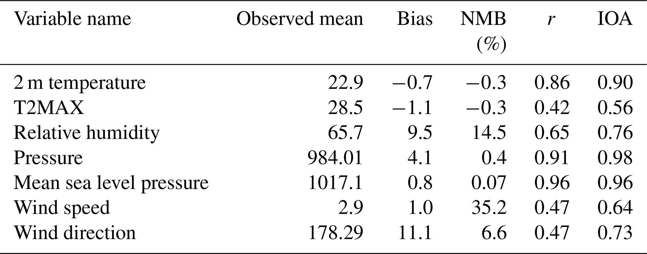
Table 3Observed mean and simulation summary statistics for meteorological parameters. The bias, normalized mean bias (NMB), correlation coefficient (r), and index of agreement (IOA) are calculated between simulated and observed meteorological parameters at the DWD stations during the 1–8 August 2018 period.
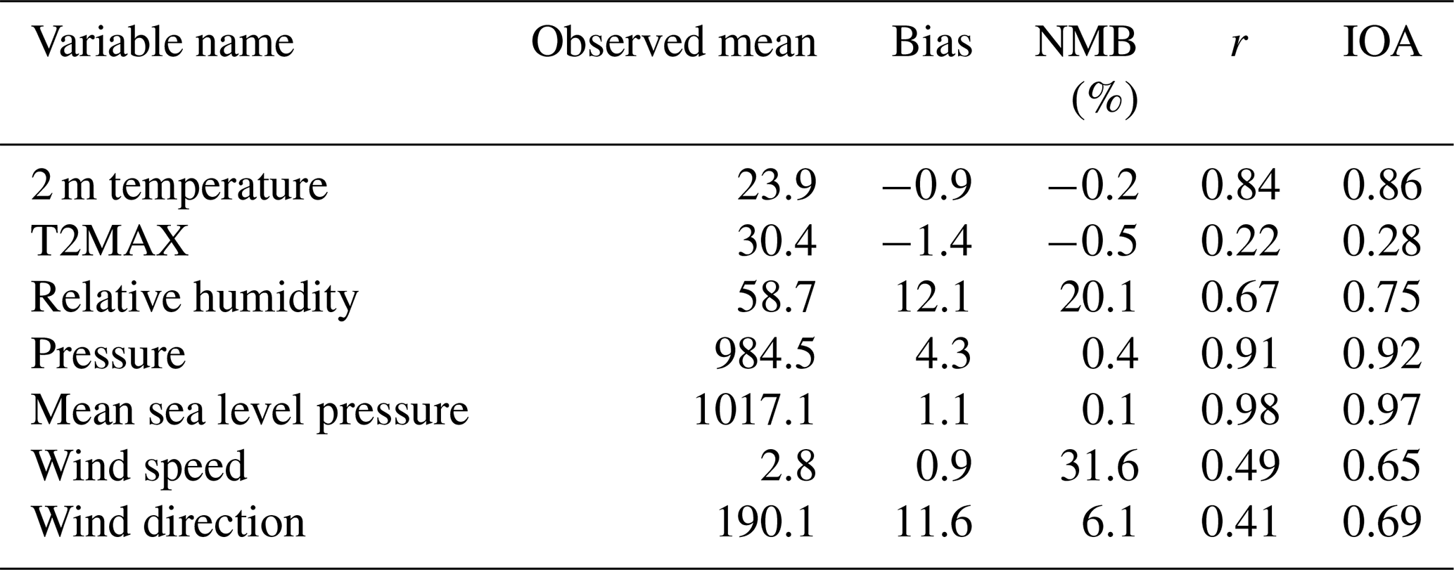
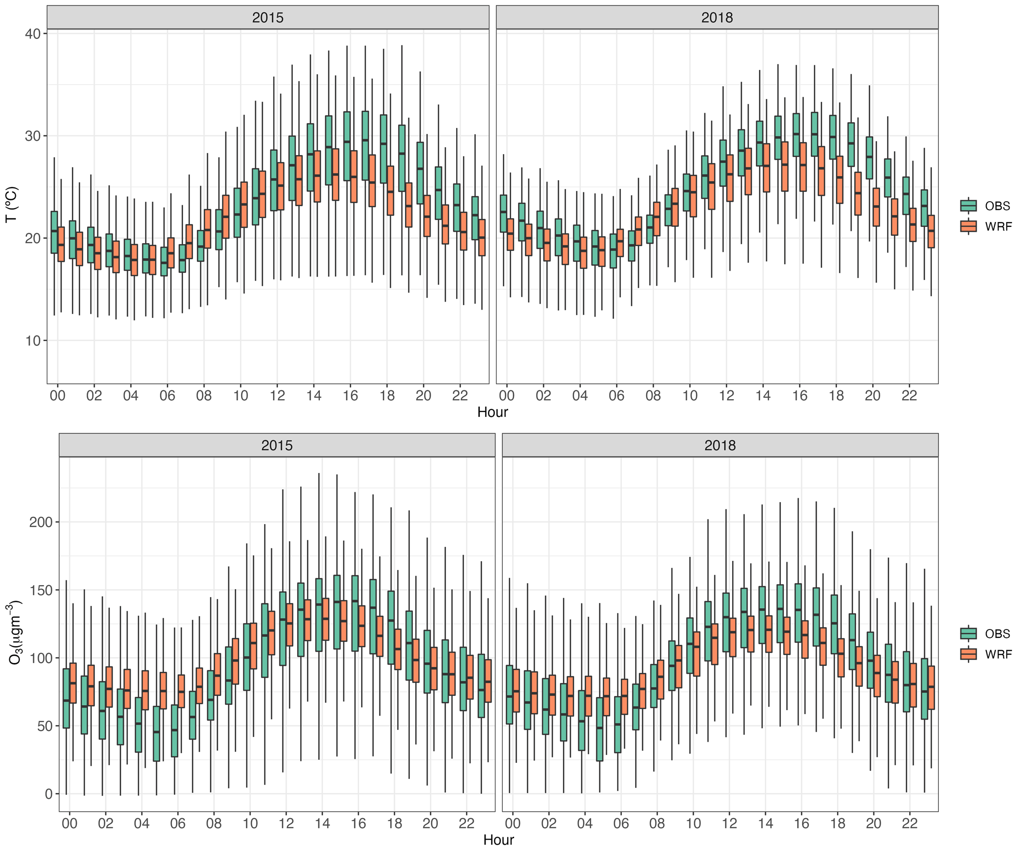
Figure 1Observed and simulated diel percentile for temperature and O3 over the analyzed periods at the German background stations. Note that the OBS temperature is given by ERA5 temperature extracted at the German background station locations. Vertical lines denote 5th and 95th percentiles, boxes denote 25th and 75th percentiles, and the black line in the boxes denotes the 50th percentiles.
Tables 4 and 5 present the evaluation for the modeled trace gases at the background sites located in the inner domain for the 2015 and 2018 simulations. These background sites include urban background, suburban background, and rural background. The model underestimates the observed concentrations and reproduces the hour-to-hour variability in NO2 and NOx reasonably well during both analyzed periods. Generally, the NO2 and NOx concentrations are slightly overestimated at the rural background stations and underestimated at suburban and urban background stations. This behavior has been also noted by Kushta et al. (2019) and Ghermandi et al. (2020). The underestimation of NOx at urban stations is mostly an effect of the spatially resolved traffic emission totals, while the overestimation at rural stations indicates that the NOx could be transported from the cities to the nearby rural areas. These discrepancies between modeled and observed NOx species could be related to the (1) errors associated with the predicted wind speed and direction, which can lead to the displacement of the modeled parcel of air relative to the observed values, (2) errors in the emissions inventory, and (3) relatively low model resolution that could lead to underestimated emission gradients and to the increased diffusion of emissions into grid cells, and therefore, the modeled grid cell concentration may not correctly represent the observed concentrations. Kuik et al. (2018) showed that, during the interval 06:00–17:00 UTC, the traffic NOx emissions could be underestimated by a factor of 3 in the urban area of Berlin, so we might assume this could be also the case for other German cities. Several other studies, such as Tuccella et al. (2012), Pirovano et al. (2012), and Georgiou et al. (2018), have also noted the overall tendency of chemical transport models to underestimate the NOx concentrations at the European level.
Table 4Observed mean and simulation summary statistics for NO2, NOx, O3, and MDA8 O3 concentrations. The bias, normalized mean bias (NMB), correlation coefficient (r), and index of agreement (IOA) are calculated between simulated and observed concentrations at the German background (all), urban and suburban backgrounds (ub), and rural (rb) stations during the 6–13 August 2015 period.
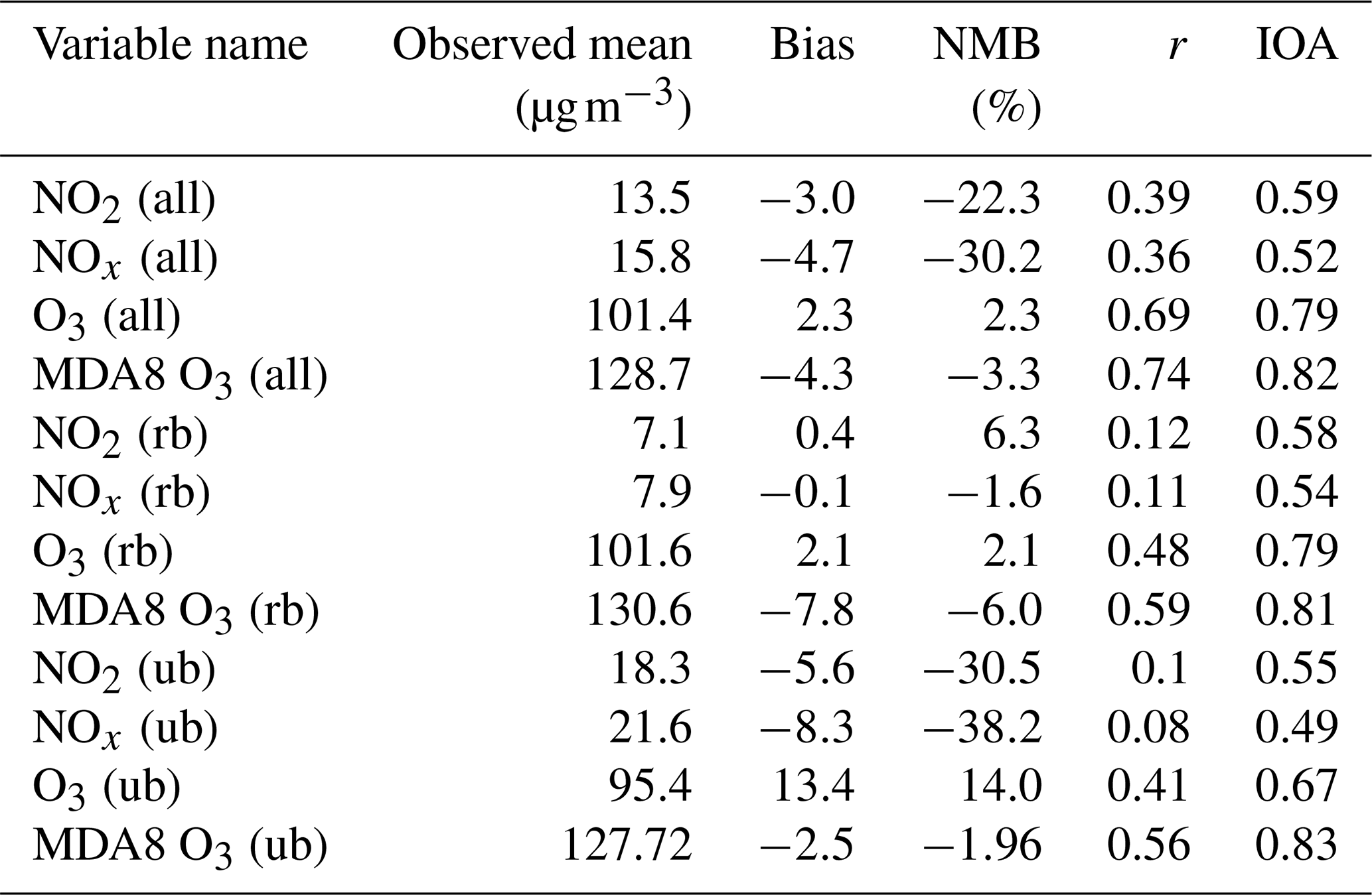
Table 5Observed mean and simulation summary statistics for NO2, NOx, O3, and MDA8 O3 concentrations. The bias, normalized mean bias (NMB), correlation coefficient (r), and index of agreement (IOA) are calculated between simulated and observed concentrations at the German background (all), urban and suburban backgrounds (ub), and rural (rb) stations during the 1–8 August 2018 period.
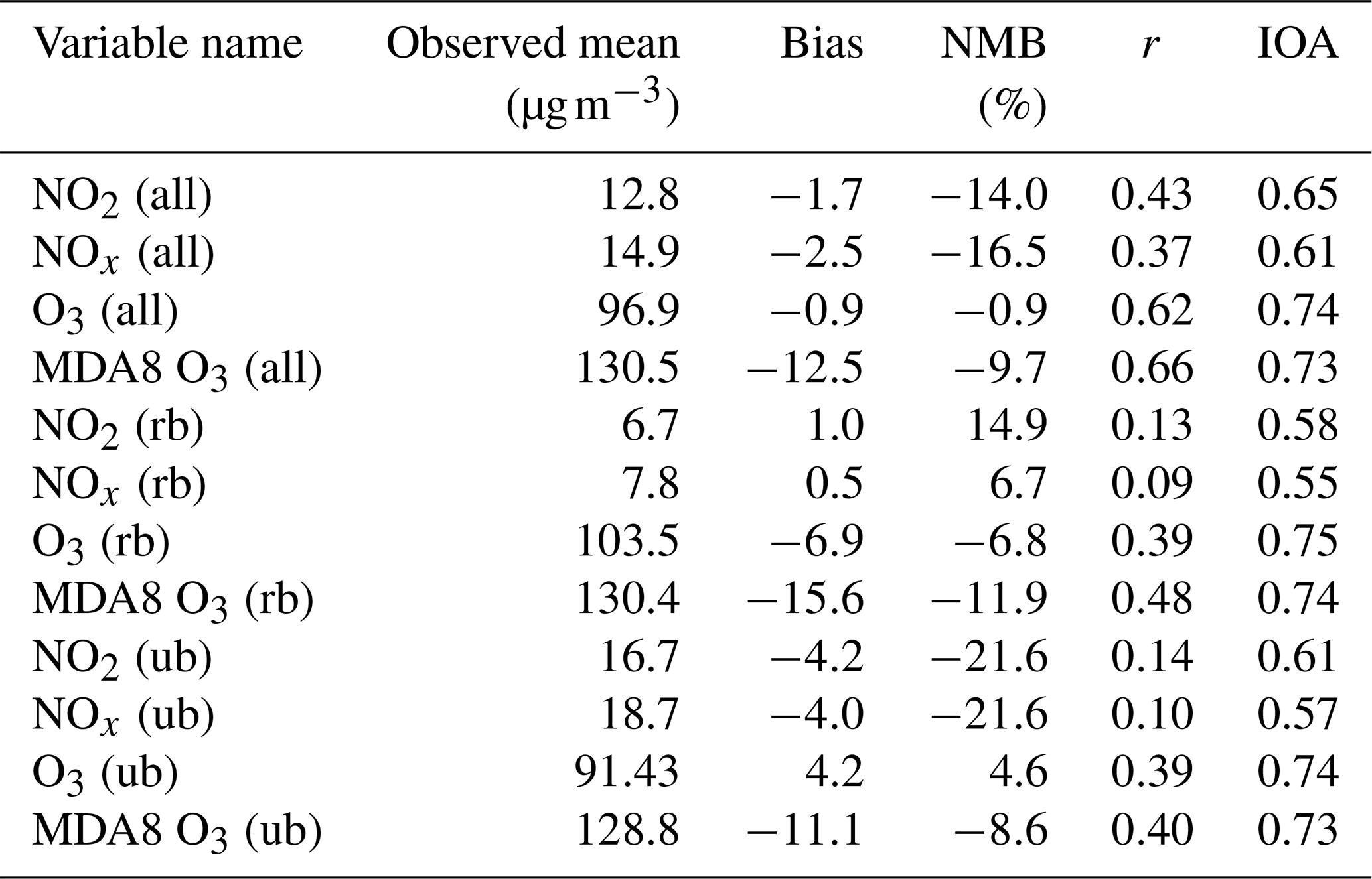
The modeled O3 concentration is quite well reproduced (NMB of 2.3 % and −0.9 % in 2015 and 2018). The lower O3 bias at rural stations compared to those seen at suburban and urban background stations could be a result of an increase in the NO titration effect due to NOx overestimation at rural stations. The comparison of hourly modeled and observed O3 at each measurement station (see also Fig. 1) reveals a persistent modeled overestimate of the nighttime concentration and an underestimation of midday concentrations. The errors in accurately predicting the meteorological inputs such as the nighttime boundary layer height could also be associated with the nighttime overprediction of surface ozone. Among the conditions that could lead to the underprediction of the ozone peak value during the daytime, we could also point to the underestimation of T2MAX, uncertainties of emissions, both from anthropogenic (NOx) and biogenic sources, and an overprediction in wind speeds that will transport the locally emitted precursors further downwind, which ultimately leads to a reduced local O3 formation rate. During AQMEII-2 (Air Quality Model Evaluation International Initiative), the working groups using WRF-Chem reported an overall underestimation of the summer O3 (Im et al., 2015). Tuccella et al. (2012) showed that, in August 2007, WRF-Chem tends to overestimate the low O3 concentrations and also underestimated those situated at the high end of the O3 concentration distribution (see their Fig. 3).
The model is biased low when predicting surface MDA8 O3 (NMB of −3.3 % and −9.7 % in August 2015 and August 2018, respectively). The temporal and spatial variability are well reproduced during these two events (r>0.74 and IOA >0.73). Since the MDA8 O3 concentrations are influenced by ozone maxima values, the consistent underestimation of peak ozone values is also noted by several models (Tuccella et al., 2012; Im et al., 2015; Oikonomakis et al., 2018; Visser et al., 2019; Mertens et al., 2020). Visser et al. (2019) showed that, in July 2015, the European mean bias for MDA8 O3 was −14.2 µg m−3, while Oikonomakis et al. (2018) noted that the model consistently underestimates the afternoon (12:00–18:00 UTC) observed O3 values above 50 ppb for the summer of 2010. Moreover, Tuccella et al. (2012) noted a mean bias (MB) for MDA8 O3 of −5 µg m−3 in 2007. Kryza et al. (2020) showed an NMB for MDA8 O3 of % during the summers of 2017 and 2018.
In summary, the model simulated the diel and multiday variation in meteorological parameters and trace gases concentrations fairly well and slightly underestimates the peaks of temperature and ozone. Nevertheless, we acknowledge that a more comprehensive evaluation would also require the comparison between modeled and observed isoprene and its oxidation products. These chemical variables play a crucial role in increasing O3 under summer conditions, but unfortunately, they are not routinely measured. Expansion of routine air quality measurements to include BVOCs or their oxidation products such as formaldehyde could significantly help with model evaluation.
4.2 Characteristics of modeled and observed surface concentration
In this section, we investigate the variability in O3 concentration levels under two different O3 peak events in Germany, focusing on the 6–13 August 2015 and 1–8 August 2018 periods and providing a possible explanation of why, although the model captures the mean O3 concentrations well, it fails in reproducing the observed O3 peaks. Table 6 shows the percentage of stations where the daily MDA8 O3 target value of 120 µg m−3 was exceeded.
Table 6Percentage of stations in each day that exceed the daily MDA8 O3 target value during the periods of 6–13 August 2015 and 1–8 August 2018.
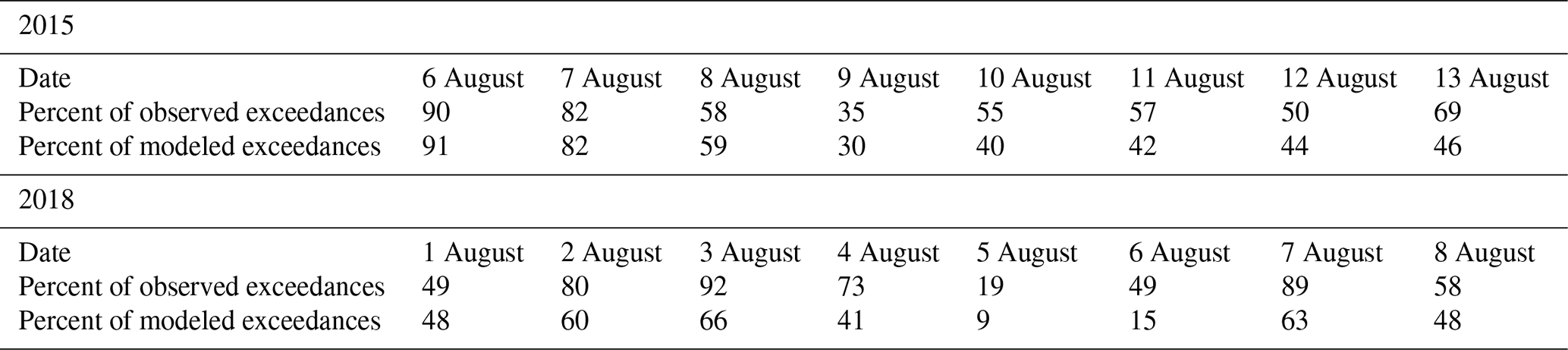
Figures 2 and 3 depict the surface maps of daily observed and modeled MDA8 O3 concentrations during the high ozone episodes. While the model captures the spatial and temporal observed pattern of MDAO3, it usually underestimates the peak of MDA8 O3 concentrations, as also shown in Table 6. This behavior is accentuated when the model fails to simulate the observed precipitation (not shown).

Figure 2Daily surface MDA8 O3 (µg m−3) for the 6–13 August 2015 period. Colored dots represent the observed MDA8 O3 concentrations at the German background stations.
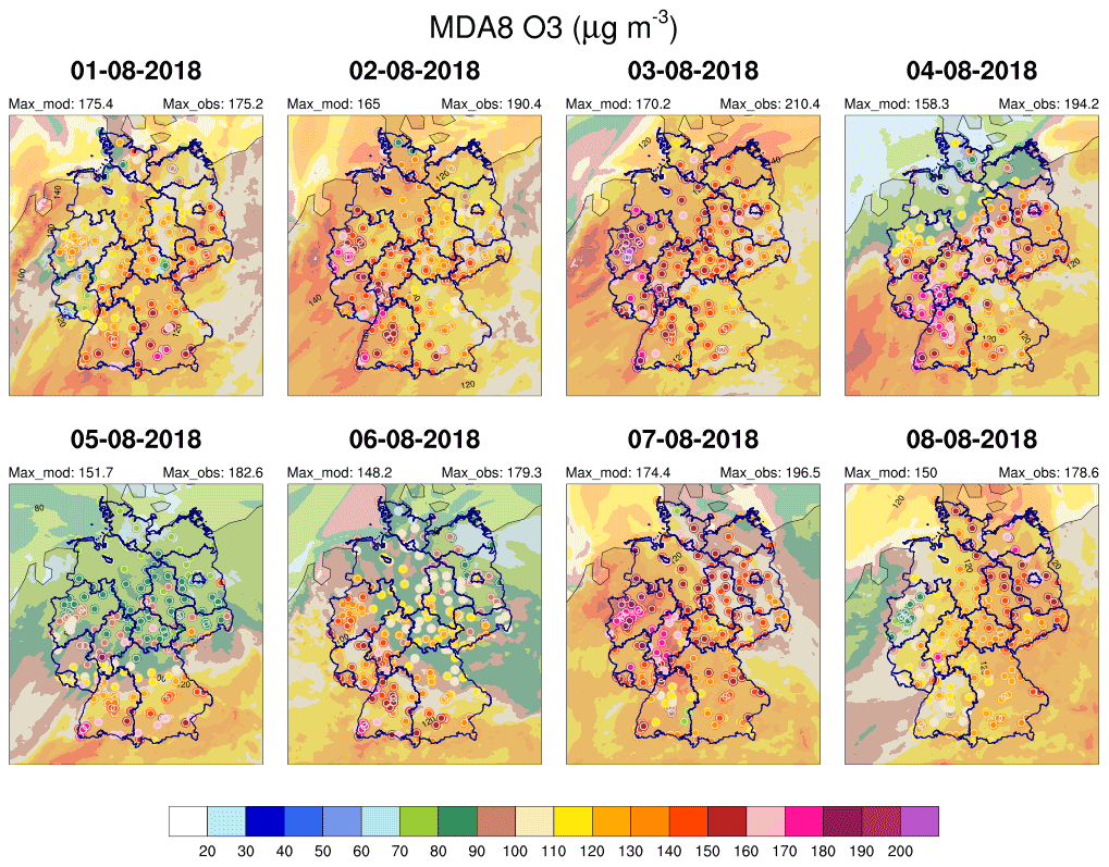
Figure 3Daily surface MDA8 O3 (µg m−3) for the 1–8 August 2018 period. Colored dots represent the observed MDA8 O3 concentrations at the German background stations.
The synoptic situation during the analyzed periods is depicted in Figs. S1 and S2 in the Supplement. Both years present similarities in their synoptic circulation patterns, although there are some small variations. In 2015, at the beginning of the period, the weather in Germany was influenced by a relatively high-pressure field situated in a saddle formed by a ridge of the Azores anticyclone and an anticyclone centered over northeastern Scandinavia. The Azores ridge, which gradually extended towards the east, was transformed into a blocking ridge over central Europe. This blocking pattern has two stagnant low-pressure systems on the edge, i.e., one in the northern Atlantic and the other over northeastern Africa. At the same time, the vertical structure was influenced by a ridge that favors the intrusion of warm tropical air coming from Africa far to the north of Europe. These ridges formed a dome of high pressure that led to stagnant weather conditions characterized by low wind speed, strong insolation and subsidence, and high temperatures. Hence, the atmospheric subsidence associated with the anticyclonic field, leading to particularly stable atmospheric conditions, contributes to explaining the elevated ozone seen over southwestern Germany in the first part of the period. As also shown in Otero et al. (2022), over Germany during the period 1999–2015, atmospheric blocking leads to temperature anomalies >5 ∘C that induce MDA8 O3 anomalies >20 µg m−3. An occluded front on 9 August 2015 led to reduced ozone values in western Germany, and it was followed by a warm front that affected northern Germany, which explains the low ozone values observed/modeled in this region. In 2018, the observed ridge of the Azores High gradually increased in magnitude, and it became centered over the middle of the Atlantic. This high-pressure field has slowly retreated towards the west; thus, the surface pressure influencing Germany became shallow and favored the appearance of a cold frontal system and moderate winds and cloudy/rainy weather that prevailed on 5–6 August 2018.
Using the scatterplots depicted in Fig. 4, we compare our modeled MDA8 O3 and the daily T2MAX pair against the observed MDA8 O3 and ERA5 T2MAX pair. We choose ERA5 T2MAX as a proxy for observed T2MAX since these measurements are not available at air quality station locations. We note that the modeled T2MAX and MDA8 O3 have relatively low correlations (r of ∼0.45); for both periods, the slopes of the linear fit to the modeled MDA8 O3 and T2MAX are comparable (3.24 and 4.04 ). When the same analysis is applied to the observed MDA8 O3 concentrations and ERA5 temperatures pair, we note a relatively high correlation of these variables (r=0.76 and 0.62) and a high ozone–temperature slope (5.6 and 5.2 ) compared to the modeled ozone–temperature slope. As previously noted, the model's failure to reproduce the meteorological variables is not conducive to O3 formation, and this could explain the model's inability to capture the observed MDA8 O3 sensitivity to T2MAX. Clearly, the underestimation of T2MAX cannot be the only factor contributing to the differences in the modeled and observed MDA8 O3-T2MAX slopes and intercept values, as +30 µg m−3 biases occur at T2MAX lower than 20 ∘C. A scatterplot of modeled vs. observed MDA8 O3 and T2MAX (see Fig. S3) shows that, generally, the T2MAX is underestimated. While the observed values of MDA8 O3 reach more than 120 µg m−3, the corresponding model values tend to be underestimated; for observed values below 75 µg m−3, the modeled values are generally overestimated. Pusede et al. (2015) have also shown that other meteorological factors, including the advection and vertical mixing, have an indirect impact on chemistry and, hence, on ozone production.
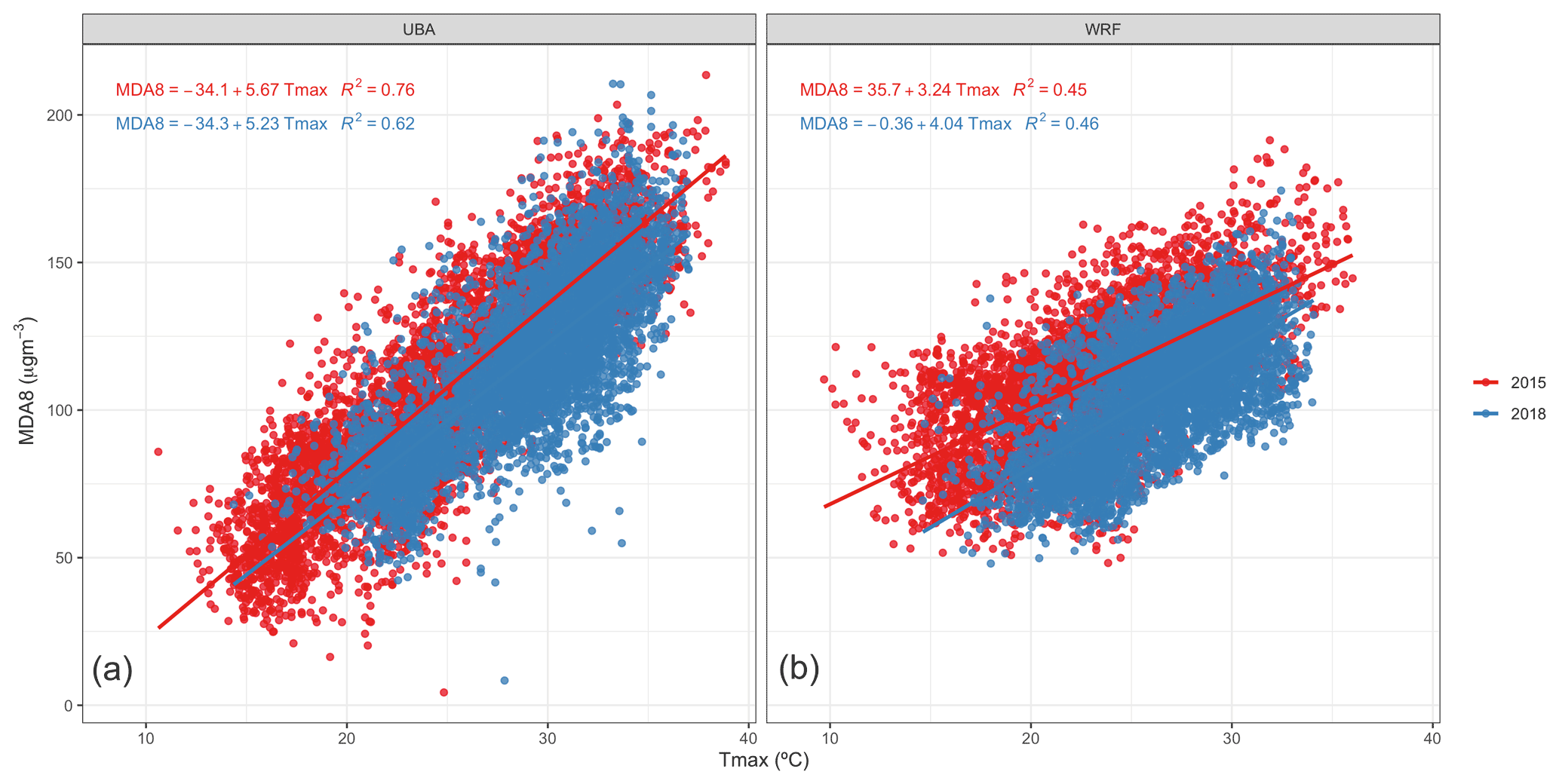
Figure 4Scatterplots showing the MDA8 O3 concentration versus the T2MAX for 2015 (red dots) and 2018 (blue dots) for all analyzed stations. Panel (a) depicts the observed MDA8 O3 vs. ERA5 T2MAX, while panel (b) exhibits the modeled MDA8 O3 and T2MAX. The solid lines are the lines of best fit.
Otero et al. (2016) showed that, in summer, apart from the temperature that is the main driver that dominates high ozone levels, relative humidity has a negative effect on ozone levels. Hence, the high modeled relative humidity (see Tables 2 and 3) together with overestimated shallow precipitation (see Figs. S4 and S5) suggest a reduction in ozone production due to enhanced cloudiness. As noted in Sect. 4.1, the overestimation of simulated wind speed could enhance the horizontal mixing of ozone and emitted pollutants in our simulations. It is well known that the ground-level ozone depends, amongst other factors, on the level of ozone precursors, such as BVOCs, especially isoprene, and anthropogenic NOx. Unfortunately, the isoprene concentrations, one of the main VOC precursors of ozone that reacts to the high NOx pathway to produce ozone, are not monitored at the German network sites, so we cannot assess the model's ability to reproduce this pollutant. Fast et al. (2014), using the measurements collected in May–June 2010 during the Carbonaceous Aerosols and Radiative Effects Study (CARES) and the California Research at the Nexus of Air Quality and Climate Change (CalNex), showed that, even if the model reproduces the temporal isoprene variation, daytime mixing ratios of isoprene are still usually a factor of 2 too low. Moreover, the underestimation of the modeled surface temperature could lead to an underestimation of isoprene emissions. Guenther et al. (2012) showed that changes in meteorology could lead to a change of ∼15 % in isoprene and terpene emission fluxes. Thus, the lack of isoprene and the underestimation of predicted NOx (see Tables 4 and 5) could also explain the underestimation of MDA8 O3.
The accurate prediction of surface ozone concentration remains a challenge because the concentration depends not only on emissions but also on a detailed representation of physical and chemical processes. Rydsaa et al. (2016) showed that WRF-Chem underestimates the modeled nighttime stomatal ozone uptake that leads to too high modeled estimates of ozone concentration in the stable nighttime planetary boundary layer. Also, they showed that, during daytime, the modeled stomatal conductance is higher than the observations and thus the midday modeled ozone concentration is too low. This is also consistent with our simulations (see Fig. 1). As in Rydsaa et al. (2016), Fig. 1 shows a low midday modeled ozone concentration, when compared with observation, and high modeled nighttime ozone. The stomatal resistance in the Wesely scheme is calculated using the first layer (surface) temperature and solar radiation. Thus, the lasting high 2 m temperature in 2018 (maximum of 34.3 ∘C and median of 21.8 ∘C) compared to those modeled in 2015 (maximum of 36.1 ∘C and median of 19.6 ∘C) leads to high stomatal resistance and, consequently, a reduced ozone uptake from vegetation that ultimately leads to an increased modeled surface concentration. Turnipseed et al. (2009) also showed that a major sink for ozone in the canopy is the direct uptake by vegetation through the stomata. Jiang et al. (2018) showed that a reduction of stomatal conductance leads to an increase in leaf temperature and, consequently, more isoprene emissions from plants. Using a global model, Gong et al. (2020) found that the O3-induced inhibition of stomatal conductance can increase surface O3 by 1.0–1.3 ppbv (parts per billion by volume) in western Europe. Visser et al. (2019) also showed that daytime stomatal conductance is overestimated. As noted in Sect. 4.1, several studies showed a systematic underestimation of WRF-Chem peak O3 values (Visser et al., 2019; Oikonomakis et al., 2018; Tuccella et al., 2012; Kryza et al., 2020). Stanier et al. (2021) noted that high MDA8 O3 values were biased low, as in our Fig. 4, while Lu et al. (2021) noted that the MDA8 O3 was, in general, underestimated in July 2018.
Moreover, as a potential effect of climate change, the high extreme temperatures in the future will hinder the O3 control; thus, knowing which sources of emissions are contributing to the severe O3 pollution episodes will help to design an effective emissions control.
4.3 Influence of different emission sources on hourly ozone at individual stations
In the following, we examine the impacts on O3 concentrations in Germany of NOx and VOC precursors for 14 individual background stations which are representative of the geographical distribution over the German states (see Table 7). Figures 5 and S6 summarize the mean absolute and relative contribution of NOx and VOC precursors to hourly surface O3 for the analyzed periods. We note that when we attribute O3 to NOx, the southern stations (Baden-Württemberg, Hesse, Rhineland-Palatinate, and Saarland) show a large contribution from the German source region (up to 35.2 µg m−3 (34.4 %) in 2015 and 33.4 µg m−3 (34.7 %) in 2018), while for the remaining station, the German NOx emissions were not seen as a dominant source, with central Europe being one of the most important contributors to the total ozone (up to 30.4 µg m−3 (29.1 %) in 2015 and 19.7 µg m−3 (22 %) in 2018). When we attribute O3 to VOC, we note that CH4 is the most significant contributor to the total O3 (up to 31.21 µg m−3 (36.3 %) in 2015 and 31.5 µg m−3 (37.2 %) in 2018), followed by German and European BVOC emissions. Furthermore, we will analyze the hourly variation in O3 concentration to examine the impact of the variation in anthropogenic and biogenic emissions, meteorology, and long-range transport. Figures 6 and 7 show the contribution of NOx precursors to hourly surface ozone in 2015 and 2018, while Figs. 8 and 9 show the contribution of VOC precursors during these periods.
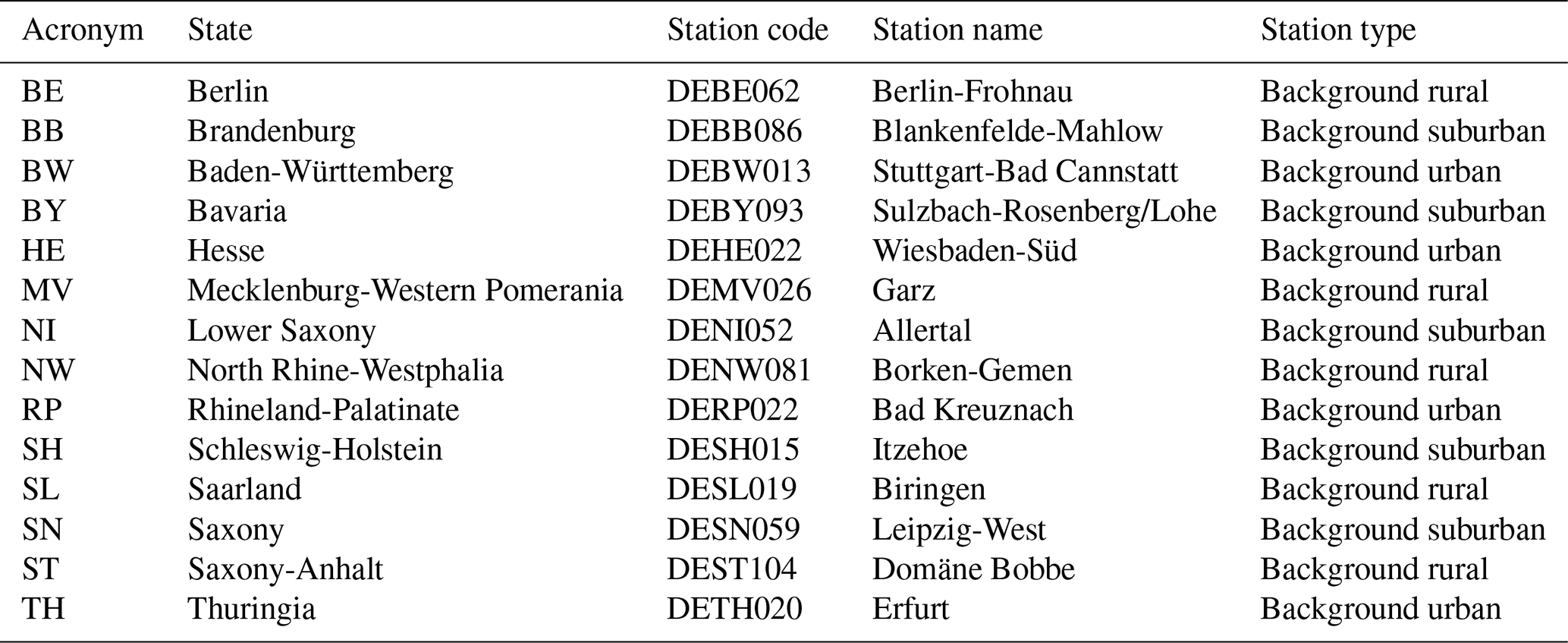
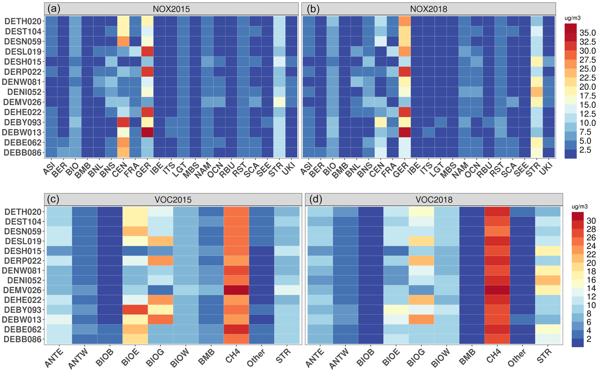
Figure 5Contribution to mean surface O3 at 14 receptor stations from local and other European sources, HTAP2 sources, and other global sources. The upper panels denote the mean contribution of NOx precursor to total O3 during 6–13 August 2015 (a) and 1–8 August 2018 (b). The bottom panels denote the mean contribution of VOC precursors to total O3 during 6–13 August 2015 (c) and 1–8 August 2018 (d).
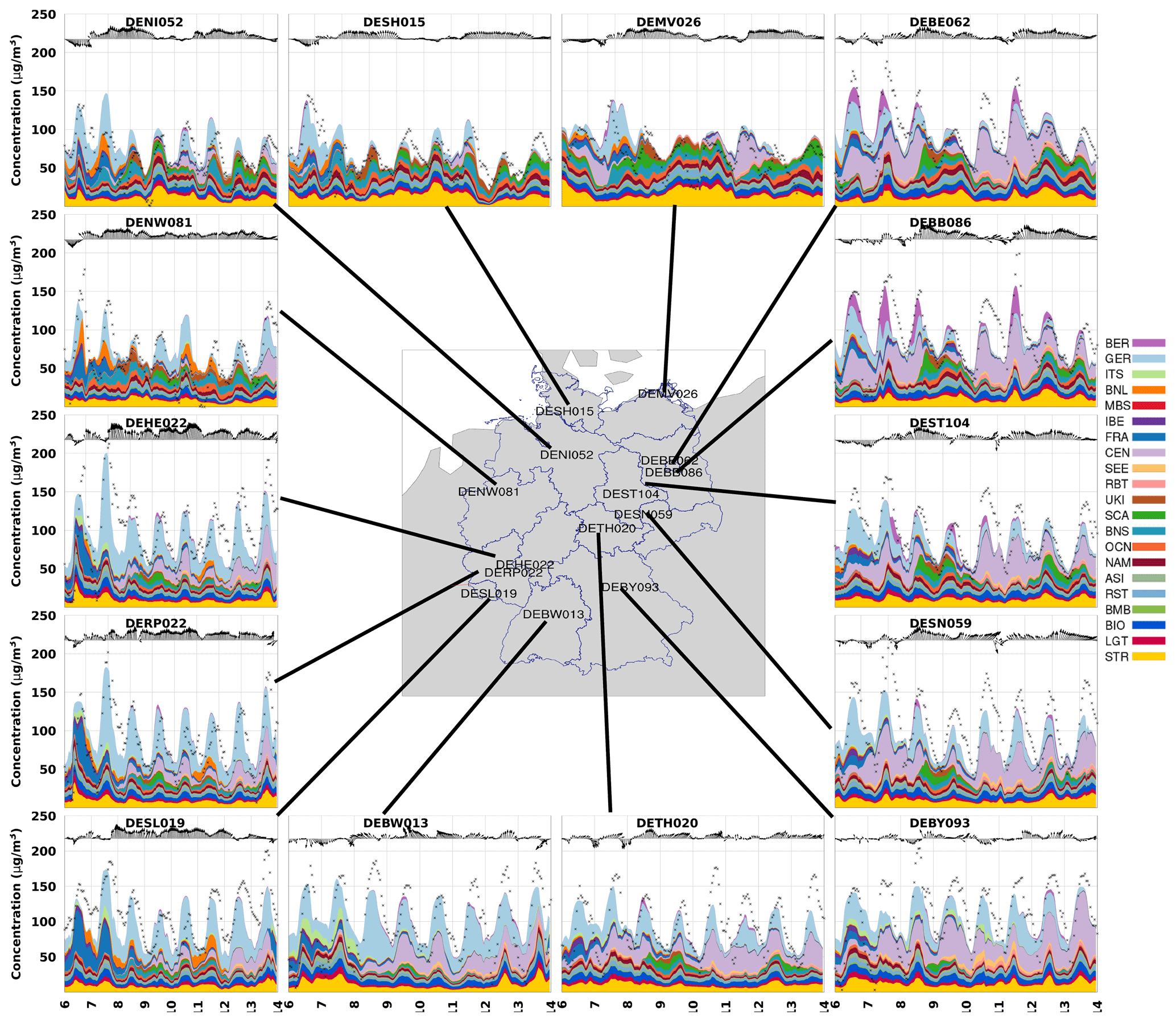
Figure 6Contribution of regional NOx sources to hourly O3 concentrations of local and other European sources, HTAP2 source regions, and other global source types at each station during the 6–13 August 2015 period. In addition, the vectors along the top of each panel represent the calculated wind speed and direction at 10 m a.g.l. The black dots represent the observed O3 concentrations.

Figure 7Contribution of regional NOx sources to hourly O3 concentrations of local and other European sources, HTAP2 source regions, and other global source types at each station during the 1–8 August 2018 period. In addition, the vectors along the top of each panel represent the calculated wind speed and direction at 10 m a.g.l. The black dots represent the observed O3 concentrations.
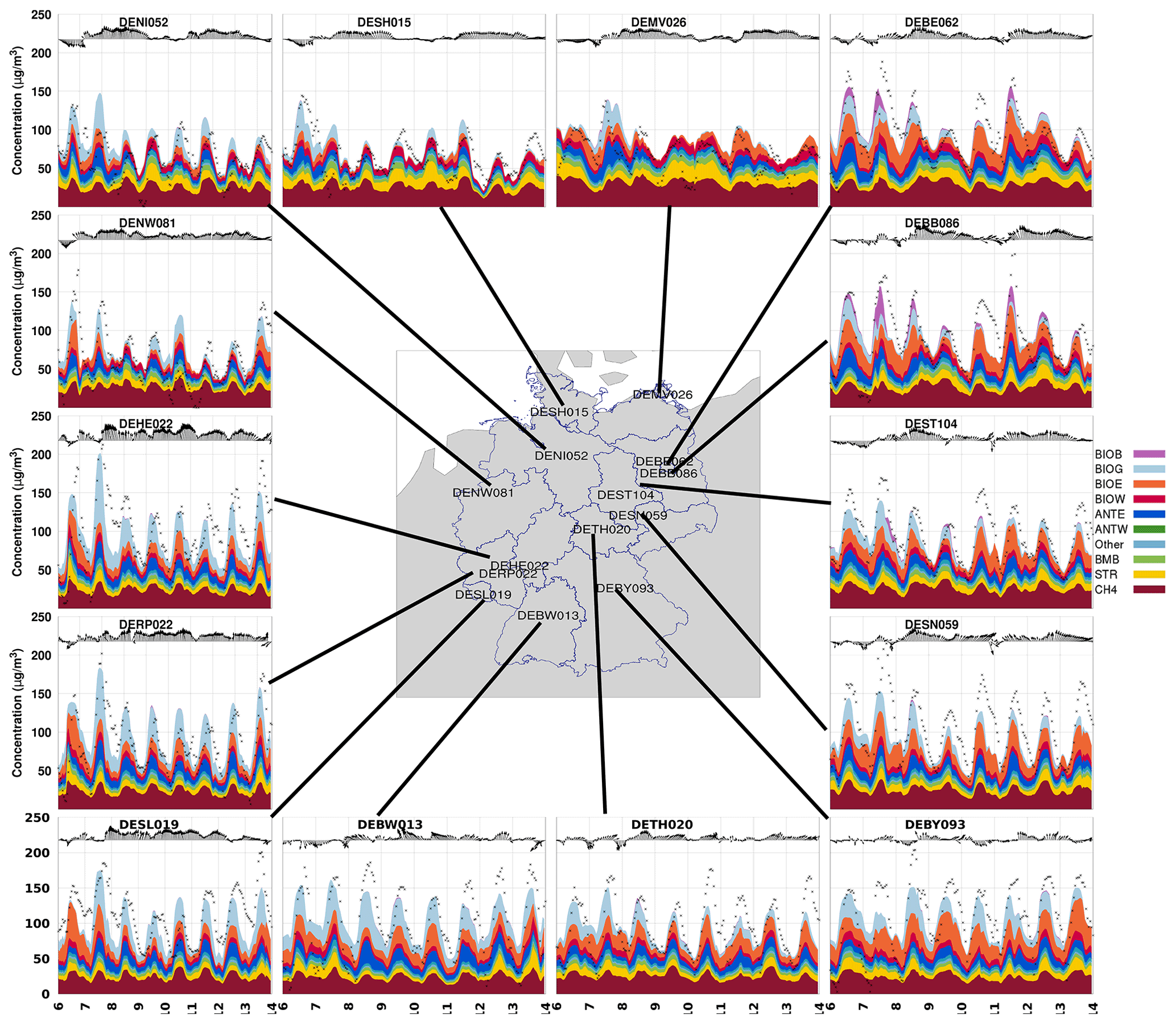
Figure 8Contribution of regional VOC sources to hourly O3 concentrations of local and other European sources, HTAP2 source regions, and other global source types at each station during the 6–13 August 2015 period. In addition, the vectors along the top of each panel represent the calculated wind speed and direction at 10 m a.g.l. The black dots represent the observed O3 concentrations.
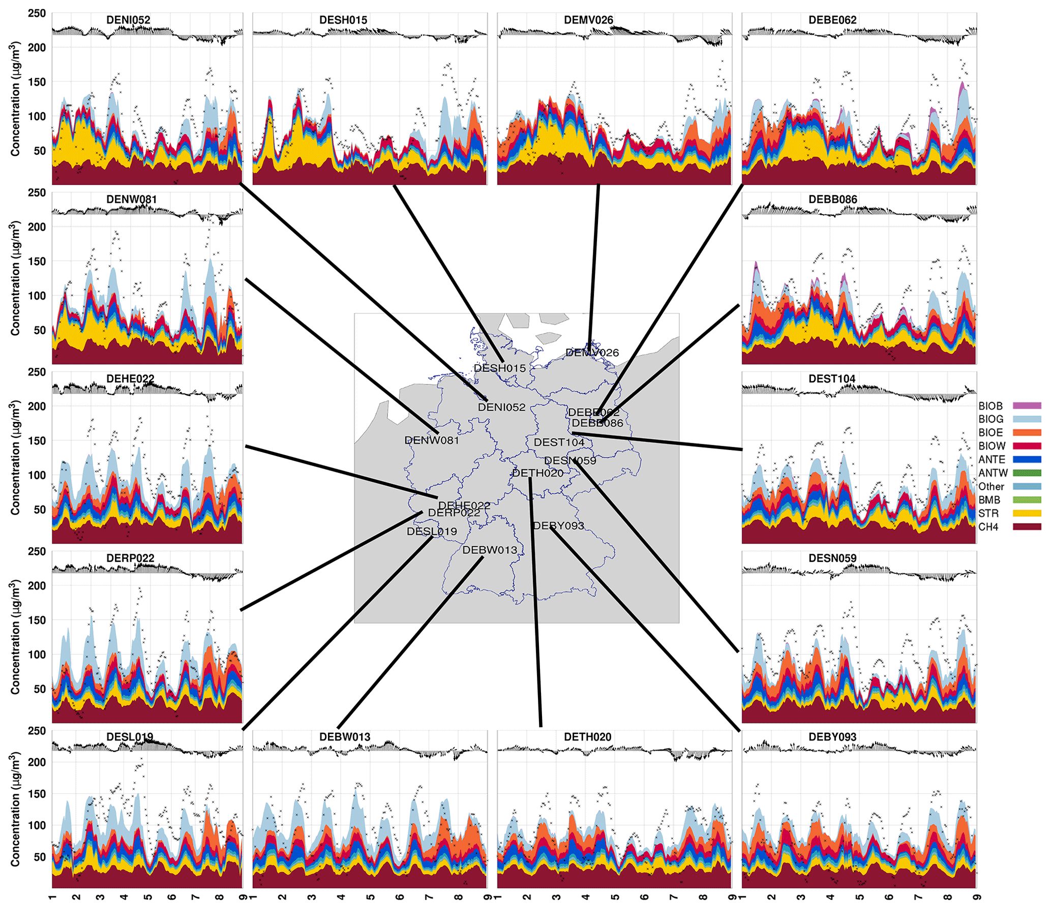
Figure 9Contribution of regional VOC sources to hourly O3 concentrations of local and other European sources, HTAP2 source regions, and other global source types at each station during the 1–8 August 2018 period. In addition, the vectors along the top of each panel represent the calculated wind speed and direction at 10 m a.g.l. The black dots represent the observed O3 concentrations.
The stratospheric contribution is similar in both simulations. Considering that the stratospheric ozone is advected within the domain through the lateral boundaries, the small differences in the stratospheric contribution noticed between the NOx and VOC-tagged simulations are related to the difference coming from CAM-Chem, as explained by Butler et al. (2018). The attribution of O3 to different sources helps to identify the ozone from the stratosphere–troposphere exchange. For both analyzed events, the variability revealed periods in which the stratospheric ozone contribution can reach 70 µg m−3 (53 %). As an example, the intrusion of stratospheric ozone seen at the beginning of August 2018 in northern Germany can be associated with the Icelandic Low that reached its minimum pressure and geopotential height on 30 July 2018, which led to a strong downward wind component and, therefore, an increase in stratospheric ozone transported to the surface (see Fig. S2). As shown in Lupaşcu and Butler (2019), the surface stratospheric O3 is attributed to the transport of stratospheric O3 concentrations that originates from the lateral boundary concentrations (taken from the CAM-Chem extended model). Clockwise winds at the edge of the Azores High brought air pollutants such as stratospheric ozone and its precursors from Iceland and the northern Atlantic to northern Germany. The blocking situation impedes the westerly winds; therefore, the transport of stratospheric ozone decreased. Kalabokas et al. (2013) showed that summer ozone maxima in Cyprus are observed when air masses that contain very high ozone concentrations subside from the upper troposphere, and consequently, they transport stratospheric O3. Similarly, our study shows that the stratospheric ozone may also have a large influence when the MDA8 O3 peak values are observed for the northern regions of Germany. Yet, the prevailing southerly winds modeled in southern Germany block the transport of stratospheric ozone in these regions. Future work should examine the stratospheric O3 intrusion and their impact on tropospheric O3 ozone production.
4.3.1 Attribution of ozone to NOx emissions
Figures 6 and 7 show the German and remote contribution of NOx emissions to hourly O3 at individual stations in different German states and the observed O3 concentrations and modeled wind speed and direction. The time series of observed O3 concentrations were captured well by the model, although it fails to reproduce the high end of the observed O3 values, as noted above. It can also be seen that the contribution of different NOx source regions and source types to the ozone time series at each station varies greatly over time and space. The average contributions of the global HTAP2 regions associated with long-range transport were ∼20 % to the total O3 and remained relatively stable in both years. Emissions from lightning and biogenic NOx have the least contributions to total O3 during these episodes.
For both episodes, the contribution of German NOx emissions to the ozone concentration is small most of the time in the northern states (from 6.7 µg m−3 (6 %) in 2015 and 7.6 µg m−3 (8.3 %) in 2018 in Mecklenburg-Western Pomerania to 9.0 (16 %) in 2015 and 12.5 µg m−3 (13.1 %) in 2018 in Brandenburg), whereas the peak ozone events in the southwestern and western German stations are mainly driven by German NOx sources (up to 35.31 µg m−3 (33.6 %) in 2015 and 33.5 µg m−3 (33.4 %) in Baden-Württemberg) usually exceeding the total contribution of the surrounding source regions. The peak ozone events in the southern states are also generally higher than the peak ozone events in the northern states. At the analyzed stations, a significant positive correlation between ozone from local NOx sources and total ozone is found in both years (r of 0.57 in Bavaria to 0.89 in Thuringia in 2015 and 0.33 in Mecklenburg-Western Pomerania to 0.84 in Saxony-Anhalt in 2018). This emphasized the importance of NOx German sources as a key factor that drives high levels of O3. These results further revealed that the high contribution of NOx German sources to hourly O3 is strongly connected with low wind speed values, endorsing the impact of high-pressure systems on serious local O3 pollution. Furthermore, we note that high wind speeds bring O3 pollution from regions upwind of the location of our stations.
The main NOx contributors to the stations differ when we compare the O3 pollution episodes in 2015 with those in 2018. As can be seen in Figs. 6 and 7, in 2015, the stations in Lower Saxony, North Rhine-Westphalia, Rhineland-Palatinate, Hesse, and Saarland are influenced by transport from sources in Benelux (up to 30 µg m−3; 31.7 %), France (up to 63 µg m−3; 48.6 %), and Italy–Switzerland (up to 22 µg m−3; 14.8 %) at the beginning of the analyzed period, while in 2018 the same source regions have a significant contribution to the same stations at the end of the analyzed period of up to 41 µg m−3 (28.9 %), 57 µg m−3 (42.9 %), and 29 µg m−3 (33.7 %), respectively. The prevailing winds that favor the influence of these source regions are from the southwest. If the dominant wind direction is from the south, then the German sources can explain more than 50 % of the total O3. Among stations in northern Germany (Schleswig-Holstein, Mecklenburg-Western Pomerania, Berlin, and Brandenburg) we note a sporadic contribution from the Scandinavian Peninsula (SCA) and the Baltic and North seas (BNS) in both years.
The outflow of ozone from other European regions plays a significant role in ozone pollution episodes, as the wind direction shifts from one day to another. Central Europe (CEN) is responsible for a remarkably constant share of ∼25 % (ranging from 19 to 30 µg m−3) of the total ozone in 2015 at stations in Berlin, Brandenburg, Saxony-Anhalt, Thuringia, Saxony, and Bavaria, while in 2018 it exhibits an erratic contribution to the total O3 concentration (see Figs. 6 and 7). Among stations within Baden-Württemberg, Bavaria, and Saxony, we distinguish a noticeable influence from the rest of the world (up to 32 µg m−3; 23 %) and RBT (Russia, Belarus, Ukraine, Republic of Türkiye, Azerbaijan, Armenia, and Georgia; up to 15 µg m−3; 13.8 %) in 2018 and of SEE (Bulgaria, Romania, Moldova, Albania, Slovenia, Croatia, Serbia, Montenegro, Macedonia, Greece, and Cyprus; up to 10 µg m−3; 11 %) in 2015. The large contribution of German and European sources during these events indicates that a reduction in high O3 pollution could not be achieved without a regional collaboration of controlling emissions sources within Europe. However, we note that the transport of ozone and its precursors could be exacerbated since our model does not capture the stagnant conditions and overestimates the wind speeds observed in calm wind conditions by more than 60 % in both years.
Even though we identified the main source regions that could explain the origin of O3 in different regions of Germany when the NOx tagged mechanism is employed, we note that there is a large variability within the same region. For example, in 2018, in Brandenburg, the contribution of the stratospheric ozone is higher in the northern area of this region in comparison with the southern area (see Fig. S7). In Baden-Württemberg (Fig. S7), the stations located in the east of the region are largely influenced by CEN (central Europe), while those located in the west exhibit the largest contribution from German sources and FRA (France).
Moreover, the simulations accounting for two pollution episodes occurring in 2 different years show that changes in circulation patterns between those 2 years can affect the contribution of different NOx emission sources to total O3. Mitigation measures targeting anthropogenic NOx emissions for the reduction in ambient ozone should focus on widespread regional reductions rather than targeted local reductions.
Shipping activities in the Baltic and North seas have also contributed to the hourly O3 (see Figs. 6, 7). This is consistent with previous work (i.e., Lupaşcu and Butler, 2019; Pay et al., 2019; Aksoyoglu et al., 2016; Jonson et al., 2020) that highlighted the impact of shipping on ozone production near coastal regions. Apart from reinforcing the role of shipping on ozone predicted in coastal areas, our ozone attribution also shows that the inland regions, such as Bavaria and Baden-Württemberg are also impacted by ozone produced from the emissions of ships (up to 3.7 µg m−3 (3.8 %) and 4.7 µg m−3 (5.2 %), respectively, in 2015 and 7.2 µg m−3 (6.6 %) and 9 µg m−3 (9.8 %) in 2018). This underlines the effect of transport of O3 produced from possibly remote NOx emissions on total O3 for mitigation purposes.
4.3.2 Attribution of ozone to VOC emissions
At the same stations, we investigate the impacts of VOC precursors on O3 concentrations in Germany (see Figs. 8 and 9). As in Butler et al. (2020a), methane oxidation is one of the main contributors to the total ozone, and it has an almost constant contribution throughout the analyzed periods, ranging from 23.3±5.8 µg m−3 (22.7±2.3 %) to 31.2±5.5 µg m−3 (36.4±5.9 %) in 2015 and from 25.6±6.4 µg m−3 (33.7±7.3 %) to 31.4±8.4 µg m−3 (38.3±9 %) in 2018. Most of the ozone from CH4 and CH4 itself is coming from the lateral boundaries. Even though we consider the domain-wide methane emissions in our system, we expect, as in Butler et al. (2020b), that the highest share of ozone coming from methane to be attributed to intercontinental transport. European anthropogenic VOC sources contribute only modestly to the O3 concentration, with an average contribution of 9.3±5 µg m−3 (10±3.6 %) in 2015 and 7.9±4.7 µg m−3 (8.6±3.9 %) in 2018. Apart from the stratospheric intrusion event in 2018, most of the spatial and temporal variability in peak ozone is driven by the production of ozone from BVOC emissions. The ozone attributed to BVOC emissions also exhibits a geographical pattern, as for the NOx tagged simulations. The highest share of ozone from biogenic sources is modeled in the south and southwest of Germany, where peak ozone is also generally higher, as noted for NOx source attribution. This region is mostly covered by broadleaf deciduous trees (EEA, 2006), a vegetation class that has especially high isoprene emissions (Guenther et al., 2006; Pfister et al., 2008). The high temperatures and the large coverage of biogenic-emitting species in the aforementioned areas can explain the high levels of ozone in these regions. The contribution of BVOCs to total O3 is higher during the day, reflecting the onset of BVOC emissions that, combined with the high temperatures, promotes the photochemical production of O3 from NOx and VOC precursors. A comparison of high ozone events in Figs. 6 and 7 with the corresponding events in Figs. 8 and 9 (see also Figs. S8 and S9) shows that BVOCs contribute to O3 when they react with anthropogenic NOx from nearby sources.
As for NOx tagging, the ozone coming from German biogenic emissions correlates relatively well with the total ozone in both years (r of 0.68 in Mecklenburg-Western Pomerania to 0.88 in Lower Saxony in 2015 and 0.43 in Mecklenburg-Western Pomerania to 0.80 in Hesse in 2018). Similar to NOx source attribution, we note that the outflow of ozone coming from biogenic sources from the rest of Europe has a considerable impact on ozone concentration seen at these stations. Moreover, at the analyzed stations, the ozone coming from biogenic sources outside Germany also displays a good correlation with the total ozone (r of 0.48 in Mecklenburg-Western Pomerania to 0.75 in North Rhine-Westphalia in 2015 and 0.15 in Saarland to 0.62 in 2018 in Thuringia). The low correlation between ozone coming from the German NOx or VOC precursors and total ozone noticed mostly in Mecklenburg-Western Pomerania is related to a low predicted photochemistry, as also indicated by T2MAX values (not shown).
The average contribution of ozone coming from German biogenic emissions ranges from 4.65 % (4.1 µg m−3) for Mecklenburg-Western Pomerania to 25.3 % (26.1 µg m−3) for Baden-Württemberg in 2015 and from 5.6 % (4.84 µg m−3) for Mecklenburg-Western Pomerania to 24 % (23.2 µg m−3) for Baden-Württemberg in 2018, which is within the range of averaged contribution shown by Mertens et al. (2020). Mertens et al. (2020) used a source attribution method that attributes O3 to all precursors without distinguishing between NOx and VOC. They showed that, during extreme ozone events, the contribution of the land transport sector is gaining importance, and, moreover, the contribution of the biogenic emissions to ozone levels is increasing during these events. Their work indicates that 18.8±0.3 % of their modeled O3 for the June–August 2008–2010 period could be explained by the large contribution of biogenic emissions (consisting of both BVOCs and soil NOx). In contrast, our approach can separate the influence of these two distinct sources. At the analyzed stations, we find that, on average, the soil NOx emissions explain just 7 % of the modeled O3, while 37 % of the modeled O3 is attributed to all European BVOC emissions, with 14 % of the ozone due to BVOC emissions just from Germany. These findings suggest that the biogenic emissions that contribute to the high ozone levels seen in Mertens et al. (2020) are mainly attributed to the BVOCs and not to the soil NOx. Our focus on peak ozone episodes favors the enhancement of biogenic emissions and, consequently, of the predicted O3 attributed to those sources. Furthermore, Pay et al. (2019) used an O3 source apportionment method that used all precursors in a single run and utilized the ratio to determine if O3 is sensitive to VOCs or NOx. They showed that their source sector, which includes biogenic emissions, could explain up to 8 % of daily mean modeled O3 during days when the O3 target values of 120 µg m−3 are exceeded in Spain. The relatively low contribution of biogenic sources to daily mean O3 suggests that their region of interest was mostly in a NOx-limited regime throughout the simulation. Moreover, their study highlighted the need to attribute the BVOCs to an individual source since these emissions represent 70 % of VOC emissions in Spain. Our source attribution method allows us to investigate the contributions of these specific emission sources to ozone, and in addition, we can separate contributions from biogenic emissions of NOx or VOC precursors on ozone levels. Our method also allows a direct quantification of O3 coming from BVOCs in comparison with other studies in which the emissions of BVOCs were simply turned on and off (i.e., Lee et al., 2014; Churkina et al., 2017; Sun et al., 2021).
Figure 10 shows the relative contribution of BVOC and its precursors from Germany and the rest of Europe to ozone peak events in the hot spot area of Baden-Württemberg, where the average predicted ozone concentration is 115 and 102 µg m−3 in 2015 and 2018, respectively. These results are averaged over each grid cell defined as Baden-Württemberg. The average contribution of ozone from German biogenic emissions is higher than 20 µg m−3 (∼23 %) in both years (see Fig. 10). We note that the temporal variation in total O3 and O3 coming from German BVOC emissions is in good agreement (r of 0.72 and 0.65). The German isoprene concentrations predicted in Baden-Württemberg build up in the early morning and evening and are low during the daytime due to the reaction with OH that ultimately leads to ozone formation in the area. Moreover, the ratio is higher during daytime (not shown), and it favors the production of O3 by NOx, leading to an enhanced O3 formation from German and other European biogenic sources. On the other hand, Fig. 10 also shows that the diurnal variation in the ozone coming from German biogenic sources is not dominated by the diurnal variation in biogenic isoprene emissions, and the peaks of ozone from biogenic sources are disconnected from local emission peaks. These findings suggest that the formation of O3 from isoprene oxidation takes place either in the vicinity of the source or occurs in the regions downwind of Baden-Württemberg. Hence, the Baden-Württemberg BVOC emissions are not the sole factor influencing ozone formation, and other meteorological and chemical processes affect the diel variation in ozone with a biogenic origin. Furthermore, Fig. 10 depicts a relatively stable contribution of ozone coming from biogenic sources originating outside of Germany (on average 18.6 µg m−3 (16.4±3.7 %) and 13.8 µg m−3 (13.3±8.7 %) in 2015 and 2018, respectively) to the baseline ozone, which is a consequence of the long ozone lifetime and the horizontal transport of ozone to Baden-Württemberg. Given the uncertainties in biogenic emissions estimates (Zhao et al., 2016; Zhang et al., 2021), a future study should include the use of MEGAN v2.1, as described by Zhao et al. (2016).
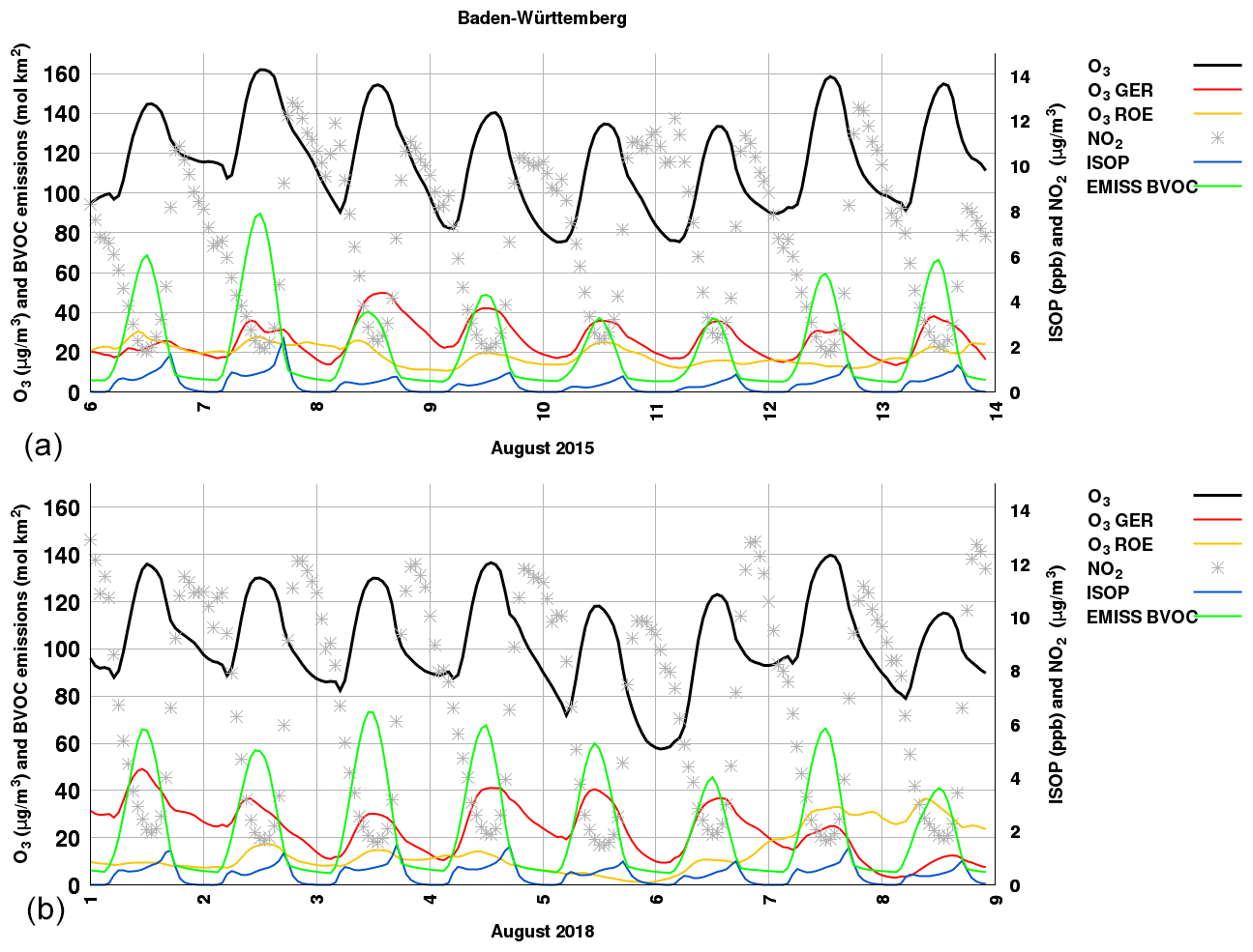
Figure 10Diurnal variation in total ozone and its German and European components together with the total BVOC emissions and isoprene concentration for 6–13 August 2015 (a) and 1–8 August 2018 (b).
The WRF-Chem model was used to perform a source attribution of German surface ozone from emitted NOx and VOC during two peak ozone events that took place in 2015 and 2018. The results from our simulations demonstrate that the peak ozone concentrations, which are reached during episodes of high temperatures, can be primarily attributed to nearby emissions of anthropogenic NOx (from Germany and its adjacent neighbors) and biogenic VOCs. Outside of these high ozone episodes, baseline ozone concentrations are attributed primarily to long-range transport, with ozone due to remote anthropogenic NOx emissions, and methane oxidation adding to the tropospheric ozone background. Anthropogenic NMVOC emissions do not contribute significantly to peak ozone events but rather make a modest contribution to the baseline ozone.
The attribution of modeled O3 to NOx emissions at 14 stations in Germany showed that, depending on the geographical location of stations, the nearby sources could have a significant contribution to ozone formation (mostly in southern Germany), whereas in northern Germany the high ozone concentrations are associated with the enhancement of transported ozone or are brought from aloft. Westerly stations are more prone to also being influenced by ozone transported from France and Benelux, while easterly stations show a constant share of O3 transported from central Europe, which is more pronounced in 2015, highlighting the importance of prevailing winds on ozone pollution levels at a given location. When attributing modeled O3 to VOC emissions, we find that the German biogenic emissions account for the largest fraction of ozone during these episodes, and they exhibit the same geographical pattern as for NOx source attribution, stressing that the production of ozone depends on the local interplay between NOx and VOC precursors. Our study also highlights the good correlation between ozone coming from German biogenic emissions and total ozone, although the diurnal variation in the ozone coming from biogenic sources is not dominated by the diurnal variation in biogenic emissions, and the peaks of ozone from biogenic sources are disconnected from local emission peaks. This suggests that the formation of O3 from local German BVOC emissions is not the sole factor that influences the ozone formation, and other meteorological and chemical processes affect the diel variation in ozone with a biogenic origin. Moreover, the relatively stable contribution of ozone coming from biogenic sources originating outside Germany to the baseline ozone underscores the combination of the long lifetime and horizontal transport of ozone.
Shipping activities in the Baltic and North seas have a great impact on ozone predicted in coastal areas, yet a small amount of ozone from these sources can also be seen far inland, stressing the importance of transported ozone on pollution levels. These findings complement those of previous studies, such as Erikson et al. (2021), and references therein, that showed that regional actions are needed to reduce the peak ozone concentration during high ozone episodes. We have also shown that changes in circulation patterns between different peak O3 episodes observed in 2015 and 2018 can affect the contribution of different NOx emission sources to the total O3; as such, the same source regions significantly impact the O3 concentration at a given location at the beginning of the analyzed period in 2015 and the end of the analyzed period in 2018. Thus, the possible influence of multiple upwind source regions should be accounted for when mitigation strategies are designed.
Overall, this study provides useful findings on how emissions from local and remote sources influence the predicted O3 and MDA8 O3 during two high ozone episodes. BVOC emissions and the NOx emitted in nearby regions enhance the O3 production during episodes of higher temperatures. Given the high importance of BVOC in determining the peak ozone concentrations, the lack of VOC measurements for the evaluation of the modeled VOCs is another source of uncertainty in modeled ozone production. Previous studies highlighted that the model strongly underestimates the isoprene concentrations, leading to an underestimation of the total ozone concentration, which might be the case for our study. It is noteworthy that, apart from modeled BVOCs, other factors such as anthropogenic emissions can influence the oxidation mechanism of the BVOC used in our simulation. Thus, the use of a highly resolved emissions inventory and additional VOC measurements, including BVOC, are necessary to improve our understanding of how well the modeled ozone precursors are simulated and, consequently, the total O3 concentrations.
The main statistical metrics employed in this study are the Pearson correlation coefficient (r), mean bias (MB), normalized mean bias (NMB), and index of agreement (IOA). These statistical indicators are defined as follows, with n as the number of model–observation pairs, M as the modeled values (with the averaged modeled value), and O as the observations (with the averaged observed value), as follows:
The WRF-Chem model is publicly available at http://www2.mmm.ucar.edu/wrf/users/download/get_source.html (last access: 15 December 2020; NCAR, 2020). To access this model, the user has to register before downloading the code. The modification introduced and described in Sect. 2 and the model data can be provided upon request to the corresponding author.
The supplement related to this article is available online at: https://doi.org/10.5194/acp-22-11675-2022-supplement.
AL and TB designed the research. AL performed the model runs. The analysis of model runs was performed by AL, with input from each of the co-authors. AL drafted the paper, with contributions from all the co-authors.
At least one of the (co-)authors is a member of the editorial board of Atmospheric Chemistry and Physics. The peer-review process was guided by an independent editor, and the authors also have no other competing interests to declare.
Publisher’s note: Copernicus Publications remains neutral with regard to jurisdictional claims in published maps and institutional affiliations.
We acknowledge the use of the WRF-Chem preprocessor tools (bio_emiss and fire_emiss, mozbc) provided by the Atmospheric Chemistry Observations and Modeling Lab (ACOM) of NCAR.
This work has been hosted by IASS Potsdam, with financial support provided by the Federal Ministry of Education and Research of Germany (BMBF) and the Ministry for Science, Research and Culture of the state of Brandenburg (MWFK; grant no. 01US1701).
This paper was edited by John Orlando and reviewed by two anonymous referees.
Aksoyoglu, S., Baltensperger, U., and Prévôt, A. S. H.: Contribution of ship emissions to the concentration and deposition of air pollutants in Europe, Atmos. Chem. Phys., 16, 1895–1906, https://doi.org/10.5194/acp-16-1895-2016, 2016.
Analitis, A., Michelozzi, P., D'Ippoliti, D., De'Donato, F., Menne, B., Matthies, F., Atkinson, R. W., Iñiguez, C., Basagaña, X., Schneider, A., Lefranc, A., Paldy, A., Bisanti, L., and Katsouyanni, K.: Effects of heat waves on mortality: effect modification and confounding by air pollutants, Epidemiology, 25, 15–22, https://doi.org/10.1097/EDE.0b013e31828ac01b, 2014.
Bieser, J., Aulinger, A., Matthias, V., Quante, M., and Denier van der Gon, H. A. C.: Vertical emission profiles for Europe based on plume rise calculations, Environ. Pollut., 159, 2935–2946, https://doi.org/10.1016/j.envpol.2011.04.030, 2011.
Buras, A., Rammig, A., and Zang, C. S.: Quantifying impacts of the 2018 drought on European ecosystems in comparison to 2003, Biogeosciences, 17, 1655–1672, https://doi.org/10.5194/bg-17-1655-2020, 2020.
Butler, T., Lupascu, A., Coates, J., and Zhu, S.: TOAST 1.0: Tropospheric Ozone Attribution of Sources with Tagging for CESM 1.2.2, Geosci. Model Dev., 11, 2825–2840, https://doi.org/10.5194/gmd-11-2825-2018, 2018.
Butler, T., Lupascu, A., and Nalam, A.: Attribution of ground-level ozone to anthropogenic and natural sources of nitrogen oxides and reactive carbon in a global chemical transport model, Atmos. Chem. Phys., 20, 10707–10731, https://doi.org/10.5194/acp-20-10707-2020, 2020a.
Butler, T. M., Leitao, J., and Lupascu, A.: Consideration of methane emissions in the modelling of ozone concentrations in chemical transport models, Final report, Texte|67/2020, Umweltbundesamt, Dessau-Roßlau, 40 pp., 2020b.
Chen, F. and Dudhia, J.: Coupling an advanced land surface-hydrology model with the Penn State-NCAR MM5 modeling system. Part I: Model implementation and sensitivity, Mon. Weather Rev., 129, 569–585, 2001.
Chen, F., Liu, C., Dudhia, J., and Chen, M.: A sensitivity study of high-resolution regional climate simulations to three land surface models over the western United States, J. Geophys. Res.-Atmos., 119, 7271–7291, https://doi.org/10.1002/2014JD021827, 2014.
Churkina, G., Kuik, F., Bonn, B., Lauer, A., Grote, R., Tomiak, K., and Butler, T. M.: Effect of VOC Emissions from Vegetation on Air Quality in Berlin during a Heatwave, Environ. Sci. Technol., 51, 6120–6130, https://doi.org/10.1021/acs.est.6b06514, 2017.
Coates, J., Mar, K. A., Ojha, N., and Butler, T. M.: The influence of temperature on ozone production under varying NOx conditions – a modelling study, Atmos. Chem. Phys., 16, 11601–11615, https://doi.org/10.5194/acp-16-11601-2016, 2016.
Curci, G., Beekmann, M., Vautard, R., Smiatek, G., Steinbrecher, R., Theloke, J., and Friedrich, R.: Modelling study of the impact of isoprene and terpene biogenic emissions on European ozone levels, Atmos. Environ., 43, 1444–1455, https://doi.org/10.1016/j.atmosenv.2008.02.070, 2009.
Duane, M., Poma, B., Rembges, D., Astorga, C., and Larsen, B. R.: Isoprene and its degradation products as strong ozone precursors in Insubria, Northern Italy, Atmos. Environ., 36, 3867–3879, https://doi.org/10.1016/S1352-2310(02)00359-X, 2002.
EEA: European forest types. Categories and types for sustainable forest management and reporting, European Environment Agency, EEA Technical report No. 9/2006. ISSN 1725-2237, https://www.eea.europa.eu/publications/technical_report_2006_9 (last access: 23 November 2020), 2006.
EEA: CORINE land cover data 2006, updated, European 20 Environment Agency, Copenhagen, Denmark, http://www.eea.europa.eu/data-and-maps/data/corine-land-cover-2006-raster-3 (last access: 20 December 2020), 2014.
Erickson, L. E., Newmark, G. L., Higgins, M. J., and Wang, Z.: Nitrogen oxides and ozone in urban air: A review of 50 plus years of progress, Environ. Prog. Sustain., 39, e13484, https://doi.org/10.1002/ep.13484, 2020.
Fast, J. D., Gustafson Jr., W. I., Easter Jr., R. C., Zaveri, R. A., Barnard, J. C., Chapman, E. G., Grell, G., and Peckham, S. E.: Evolution of Ozone, Particulates, and Aerosol Direct Radiative Forcing in the Vicinity of Houston Using a Fully Coupled Meteorology-Chemistry-Aerosol Model, J. Geophys. Res., 111, D21305, https://doi.org/10.1029/2005JD006721, 2006.
Fast, J. D., Allan, J., Bahreini, R., Craven, J., Emmons, L., Ferrare, R., Hayes, P. L., Hodzic, A., Holloway, J., Hostetler, C., Jimenez, J. L., Jonsson, H., Liu, S., Liu, Y., Metcalf, A., Middlebrook, A., Nowak, J., Pekour, M., Perring, A., Russell, L., Sedlacek, A., Seinfeld, J., Setyan, A., Shilling, J., Shrivastava, M., Springston, S., Song, C., Subramanian, R., Taylor, J. W., Vinoj, V., Yang, Q., Zaveri, R. A., and Zhang, Q.: Modeling regional aerosol and aerosol precursor variability over California and its sensitivity to emissions and long-range transport during the 2010 CalNex and CARES campaigns, Atmos. Chem. Phys., 14, 10013–10060, https://doi.org/10.5194/acp-14-10013-2014, 2014.
Fiore, A. M., West, J. J., Horowitz, L. W., Naik, V., and Schwarzkopf, M. D.: Characterizing the tropospheric ozone response to methane emission controls and the benefits to climate and air quality, J. Geophys. Res., 113, D08307, https://doi.org/10.1029/2007JD009162, 2008.
Fiore, A. M., Levy II, H., and Jaffe, D. A.: North American isoprene influence on intercontinental ozone pollution, Atmos. Chem. Phys., 11, 1697–1710, https://doi.org/10.5194/acp-11-1697-2011, 2011.
Gao, M., Han, Z., Liu, Z., Li, M., Xin, J., Tao, Z., Li, J., Kang, J.-E., Huang, K., Dong, X., Zhuang, B., Li, S., Ge, B., Wu, Q., Cheng, Y., Wang, Y., Lee, H.-J., Kim, C.-H., Fu, J. S., Wang, T., Chin, M., Woo, J.-H., Zhang, Q., Wang, Z., and Carmichael, G. R.: Air quality and climate change, Topic 3 of the Model Inter-Comparison Study for Asia Phase III (MICS-Asia III) – Part 1: Overview and model evaluation, Atmos. Chem. Phys., 18, 4859–4884, https://doi.org/10.5194/acp-18-4859-2018, 2018.
Georgiou, G. K., Christoudias, T., Proestos, Y., Kushta, J., Hadjinicolaou, P., and Lelieveld, J.: Air quality modelling in the summer over the eastern Mediterranean using WRF-Chem: chemistry and aerosol mechanism intercomparison, Atmos. Chem. Phys., 18, 1555–1571, https://doi.org/10.5194/acp-18-1555-2018, 2018.
Ghermandi, G., Fabbi, S., Veratti, G., Bigi, A., and Teggi, S.: Estimate of Secondary NO2 Levels at Two Urban Traffic Sites Using Observations and Modelling, Sustainability, 12, 7897, https://doi.org/10.3390/su12197897, 2020.
Gómez-Navarro, J. J., Raible, C. C., and Dierer, S.: Sensitivity of the WRF model to PBL parametrisations and nesting techniques: evaluation of wind storms over complex terrain, Geosci. Model Dev., 8, 3349–3363, https://doi.org/10.5194/gmd-8-3349-2015, 2015.
Gong, C., Lei, Y., Ma, Y., Yue, X., and Liao, H.: Ozone–vegetation feedback through dry deposition and isoprene emissions in a global chemistry–carbon–climate model, Atmos. Chem. Phys., 20, 3841–3857, https://doi.org/10.5194/acp-20-3841-2020, 2020.
Grell, G. A., Peckham, S. E., Schmitz, R., McKeen, S. A., Frost, G., Skamarock, W. C., and Eder, B.: Fully coupled online chemistry within the WRF model, Atmos. Environ., 39, 6957–6975, 2005.
Grewe, V., Tsati, E., Mertens, M., Frömming, C., and Jöckel, P.: Contribution of emissions to concentrations: the TAGGING 1.0 submodel based on the Modular Earth Submodel System (MESSy 2.52), Geosci. Model Dev., 10, 2615–2633, https://doi.org/10.5194/gmd-10-2615-2017, 2017.
Guenther, A., Karl, T., Harley, P., Wiedinmyer, C., Palmer, P. I., and Geron, C.: Estimates of global terrestrial isoprene emissions using MEGAN (Model of Emissions of Gases and Aerosols from Nature), Atmos. Chem. Phys., 6, 3181–3210, https://doi.org/10.5194/acp-6-3181-2006, 2006.
Guenther, A. B., Jiang, X., Heald, C. L., Sakulyanontvittaya, T., Duhl, T., Emmons, L. K., and Wang, X.: The Model of Emissions of Gases and Aerosols from Nature version 2.1 (MEGAN2.1): an extended and updated framework for modeling biogenic emissions, Geosci. Model Dev., 5, 1471–1492, https://doi.org/10.5194/gmd-5-1471-2012, 2012.
Guerova, G. and Jones, N.: A global model study of ozone enhancement during the August 2003 heat wave in Europe, Environ. Chem., 4, 285–292, https://doi.org/10.1071/EN07027, 2007.
Hersbach, H. and Dee, D.: ERA5 reanalysis is in production, ECMWF Newsletter No. 147, p. 7, 2016.
Hong, S., Noh, Y., and Dudhia, J.: A new vertical diffusion package with an explicit treatment of entrainment processes, Mon. Weather Rev., 134, 2318–2341, https://doi.org/10.1175/MWR3199.1, 2006.
Hoy, A., Hänsel, S., Skalak, S., Ustrnul, Z., and Bochníček, O.: The extreme European summer of 2015 in a long-term perspective, Int. J. Climatol., 37, 943–962, https://doi.org/10.1002/joc.4751, 2016.
Hu, X.-M., Klein, P. M., and Xue, M.: Evaluation of the updated YSU planetary boundary layer scheme within WRF for wind resource and air quality assessments, J. Geophys. Res.-Atmos., 118, 10490–10505, https://doi.org/10.1002/jgrd.50823, 2013.
Iacono, M. J., Delamere, J. S., Mlawer, E. J., Shephard, M. W., Clough, S. A., and Collins, W. D.: Radiative forcing by long-lived greenhouse gases: Calculations with the AER radiative transfer models, J. Geophys. Res., 113, D13103, https://doi.org/10.1029/2008JD009944, 2008.
Im, U., Bianconi, R., Solazzo, E., Kioutsioukis, I., Badia, A.,Balzarini, A., Baró, R., Bellasio, R., Giordano, L., Jiménez-Guerrero, P., Hirtl, M., Hodzic, A., Honzak, L., Jorba, O., Knote,C., Kuenen, J. J. P., Makar, P. A., Mandes-Groot, A., Neal,L., Pérez, J. L., Pirovano, G., Pouliot, G., San Jose, R., Savage, N., Schroder, W., Sokhi, R. S., Syrakov, D., Torian, A.,Tucella, P., Werhahn, J., Wolke, R., Yahya, K., Zabkar, R.,Zhang, Y., Zhang, J., Hogrefe, C., and Galmarini, S.: Evaluation of operational on-lin-coupled regional air quality models over Europe and North America in the contex of AQMEII phase1. Part II: Particulate matter, Atmos. Environ., 115, 421–441, https://doi.org/10.1016/j.atmosenv.2014.08.072, 2015.
Ionita, M., Tallaksen, L. M., Kingston, D. G., Stagge, J. H., Laaha, G., Van Lanen, H. A. J., Scholz, P., Chelcea, S. M., and Haslinger, K.: The European 2015 drought from a climatological perspective, Hydrol. Earth Syst. Sci., 21, 1397–1419, https://doi.org/10.5194/hess-21-1397-2017, 2017.
IPCC: Managing the Risks of Extreme Events and Disasters to Advance Climate Change Adaptation. A Special Report of Working Groups I and II of the Intergovernmental Panel on Climate Change, edited by: Field, C. B., Barros, V., Stocker, T. F., Qin, D., Dokken, D. J., Ebi, K. L., Mastrandrea, M. D., Mach, K. J., Plattner, G.-K., Allen, S. K., Tignor, M., and Midgley, P. M.: Cambridge University Press, Cambridge, United Kingdom and New York, NY, USA, 582 pp., 2012.
Jacob, D. J. and Winner, D. A.: Effect of climate change on air quality, Atmos. Environ., 43, 51–63, 2009.
Janssens-Maenhout, G., Crippa, M., Guizzardi, D., Dentener, F., Muntean, M., Pouliot, G., Keating, T., Zhang, Q., Kurokawa, J., Wankmüller, R., Denier van der Gon, H., Kuenen, J. J. P., Klimont, Z., Frost, G., Darras, S., Koffi, B., and Li, M.: HTAP_v2.2: a mosaic of regional and global emission grid maps for 2008 and 2010 to study hemispheric transport of air pollution, Atmos. Chem. Phys., 15, 11411–11432, https://doi.org/10.5194/acp-15-11411-2015, 2015.
Jiang, J., Aksoyoglu, S., Ciarelli, G., Oikonomakis, E., El-Haddad, I., Canonaco, F., O'Dowd, C., Ovadnevaite, J., Minguillón, M. C., Baltensperger, U., and Prévôt, A. S. H.: Effects of two different biogenic emission models on modelled ozone and aerosol concentrations in Europe, Atmos. Chem. Phys., 19, 3747–3768, https://doi.org/10.5194/acp-19-3747-2019, 2019.
Jiang, X., Guenther, A., Potosnak, M., Geron, C., Seco, R., Karl, T., Kim, S., Gu, L., and Pallardy, S.: Isoprene emission response to drought and the impact on global atmospheric chemistry, Atmos. Environ., 183, 69–83, https://doi.org/10.1016/j.atmosenv.2018.01.026, 2018.
Jonson, J. E., Schulz, M., Emmons, L., Flemming, J., Henze, D., Sudo, K., Tronstad Lund, M., Lin, M., Benedictow, A., Koffi, B., Dentener, F., Keating, T., Kivi, R., and Davila, Y.: The effects of intercontinental emission sources on European air pollution levels, Atmos. Chem. Phys., 18, 13655–13672, https://doi.org/10.5194/acp-18-13655-2018, 2018.
Jonson, J. E., Gauss, M., Schulz, M., Jalkanen, J.-P., and Fagerli, H.: Effects of global ship emissions on European air pollution levels, Atmos. Chem. Phys., 20, 11399–11422, https://doi.org/10.5194/acp-20-11399-2020, 2020.
Kain, J. S.: The Kain-Fritsch convective parameterization: An update, J. Appl. Meteorol., 43, 170–181, 2004.
Kalabokas, P. D., Cammas, J.-P., Thouret, V., Volz-Thomas, A., Boulanger, D., and Repapis, C. C.: Examination of the atmospheric conditions associated with high and low summer ozone levels in the lower troposphere over the eastern Mediterranean, Atmos. Chem. Phys., 13, 10339–10352, https://doi.org/10.5194/acp-13-10339-2013, 2013.
Karlický, J., Huszár, P., Nováková, T., Belda, M., Švábik, F., Ďoubalová, J., and Halenka, T.: The “urban meteorology island”: a multi-model ensemble analysis, Atmos. Chem. Phys., 20, 15061–15077, https://doi.org/10.5194/acp-20-15061-2020, 2020.
Kaspar, F., Müller-Westermeier, G., Penda, E., Mächel, H., Zimmermann, K., Kaiser-Weiss, A., and Deutschländer, T.: Monitoring of climate change in Germany – data, products and services of Germany's National Climate Data Centre, Adv. Sci. Res., 10, 99–106, https://doi.org/10.5194/asr-10-99-2013, 2013.
Kehler-Poljak, G., Telišman Prtenjak, M., Kvakić, M., Šariri, K., and Večenaj, Z.: Interaction of Sea Breeze and Deep Convection over the Northeastern Adriatic Coast: An Analysis of Sensitivity Experiments Using a High-Resolution Mesoscale Model, Pure Appl. Geophys., 174, 4197–4224, https://doi.org/10.1007/s00024-017-1607-x, 2017.
Kryza, M., Werner, M., Dudek, J., and Dore, A. J.: The Effect of Emission Inventory on Modelling of Seasonal Exposure Metrics of Particulate Matter and Ozone with the WRF-Chem Model for Poland, Sustainability, 12, 5414, https://doi.org/10.3390/su12135414, 2020.
Kuenen, J. J. P., Visschedijk, A. J. H., Jozwicka, M., and Denier van der Gon, H. A. C.: TNO-MACC_II emission inventory; a multi-year (2003–2009) consistent high-resolution European emission inventory for air quality modelling, Atmos. Chem. Phys., 14, 10963–10976, https://doi.org/10.5194/acp-14-10963-2014, 2014.
Kuik, F., Lauer, A., Churkina, G., Denier van der Gon, H. A. C., Fenner, D., Mar, K. A., and Butler, T. M.: Air quality modelling in the Berlin–Brandenburg region using WRF-Chem v3.7.1: sensitivity to resolution of model grid and input data, Geosci. Model Dev., 9, 4339–4363, https://doi.org/10.5194/gmd-9-4339-2016, 2016.
Kuik, F., Kerschbaumer, A., Lauer, A., Lupascu, A., von Schneidemesser, E., and Butler, T. M.: Top–down quantification of NOx emissions from traffic in an urban area using a high-resolution regional atmospheric chemistry model, Atmos. Chem. Phys., 18, 8203–8225, https://doi.org/10.5194/acp-18-8203-2018, 2018.
Kushta, J., Georgiou, G. K., Proestos, Y., Christoudias, T., Thunis, P., Savvides, C., Papadopoulos, C., and Lelieveld, J.: Evaluation of EU air quality standards through modeling and the FAIRMODE benchmarking methodology, Air Qual. Atmos. Hlth, 12, 73–86, https://doi.org/10.1007/s11869-018-0631-z, 2019.
Lee, K.-Y., Kwak, K.-H., Ryu, Y.-H., Lee, S.-H., and Baik, J.-J.: Impacts of biogenic isoprene emission on ozone air quality in the Seoul metropolitan area, Atmos. Environ., 96, 209–219, https://doi.org/10.1016/j.atmosenv.2014.07.036, 2014.
Lin, C.-Y. C., Jacob, D. J., and Fiore, A. M.: Trends in exceedances of the ozone air quality standard in the continental United States, 1980–1998, Atmos. Environ., 35, 3217–3228, 2001.
Lin, M., Malyshev, S., Shevliakova, E., Paulot, F., Horowitz, L. W., Fares, S., Mikkelsen, T. N., and Zhang, L.: Sensitivity of ozone dry deposition to ecosystem-atmosphere interactions: A critical appraisal of observations and simulations, Global Biogeochem. Cy., 33, 1264–1288, https://doi.org/10.1029/2018GB006157, 2019.
Lin, M., Horowitz, L., Paulot, F., Malyshev, S., Shevliakova, E., Finco, A., Gerosa, G., Kubistin, D., and Pilegaard, K.: Vegetation feedbacks during drought exacerbate ozone air pollution extremes in Europe, Nat. Clim. Change, 10, 791, https://doi.org/10.1038/s41558-020-0839-4, 2020.
Lu, X., Ye, X., Zhou, M., Zhao, Y., Weng, H., Kong, H., Li, K., Gao, M., Zheng, B., Lin, J., Zhou, F., Zhang, Q., Wu, D., Zhang, L., and Zhang, Y.: The underappreciated role of agricultural soil nitrogen oxide emissions in ozone pollution regulation in North China, Nat. Commun., 12, 5021, https://doi.org/10.1038/s41467-021-25147-9, 2021.
Lupaşcu, A. and Butler, T.: Source attribution of European surface O3 using a tagged O3 mechanism, Atmos. Chem. Phys., 19, 14535–14558, https://doi.org/10.5194/acp-19-14535-2019, 2019.
Mailler, S., Khvorostyanov, D., and Menut, L.: Impact of the vertical emission profiles on background gas-phase pollution simulated from the EMEP emissions over Europe, Atmos. Chem. Phys., 13, 5987–5998, https://doi.org/10.5194/acp-13-5987-2013, 2013.
Meehl, G. A., Tebaldi, C., Tilmes, S., Lamarque, J. F., Bates, S., Pendergrass, A., and Lombardozzi, D.: Future heat waves and surface ozone, Environ. Res. Lett., 13, 064004, https://doi.org/10.1088/1748-9326/aabcdc, 2018.
Mertens, M., Kerkweg, A., Grewe, V., Jöckel, P., and Sausen, R.: Attributing ozone and its precursors to land transport emissions in Europe and Germany, Atmos. Chem. Phys., 20, 7843–7873, https://doi.org/10.5194/acp-20-7843-2020, 2020.
Morrison, H., Thompson, G., and Tatarskii, V.: Impact of cloud microphysics on the development of trailing stratiform precipitation in a simulated squall line: comparison of one- and two-moment schemes, Mon. Weather Rev., 137, 991–1007, https://doi.org/10.1175/2008MWR2556.1, 2009.
NCAR: WRF-Chem model, NCAR, http://www2.mmm.ucar.edu/wrf/users/download/get_source.html, last access: 15 December 2020.
Oikonomakis, E., Aksoyoglu, S., Ciarelli, G., Baltensperger, U., and Prévôt, A. S. H.: Low modeled ozone production suggests underestimation of precursor emissions (especially NOx) in Europe, Atmos. Chem. Phys., 18, 2175–2198, https://doi.org/10.5194/acp-18-2175-2018, 2018.
Ordóñez, C., Elguindi, N., Stein, O., Huijnen, V., Flemming, J., Inness, A., Flentje, H., Katragkou, E., Moinat, P., Peuch, V.-H., Segers, A., Thouret, V., Athier, G., van Weele, M., Zerefos, C. S., Cammas, J.-P., and Schultz, M. G.: Global model simulations of air pollution during the 2003 European heat wave, Atmos. Chem. Phys., 10, 789–815, https://doi.org/10.5194/acp-10-789-2010, 2010.
Orth, R., Zscheischler, J., and Seneviratne, S. I.: Record dry summer in 2015 challenges precipitation projections in Central Europe, Scientific Reports, 6, 28334, https://doi.org/10.1038/srep28334, 2016.
Otero, N., Sillmann, J., Schnell, J. L., Rust, H. W., and Butler, T.: Synoptic and meteorological drivers of extreme ozone concentrations over Europe, Environ. Res. Lett., 11, 024005, https://doi.org/10.1088/1748-9326/11/2/024005, 2016.
Otero, N., Jurado, O. E., Butler, T., and Rust, H. W.: The impact of atmospheric blocking on the compounding effect of ozone pollution and temperature: a copula-based approach, Atmos. Chem. Phys., 22, 1905–1919, https://doi.org/10.5194/acp-22-1905-2022, 2022.
Otu-Larbi, F., Bolas, C. G., Ferracci, V., Staniaszek, Z., Jones, R. L., Malhi, Y., Harris, N. R. P., Wild, O., and Ashworth, K.: Modelling the effect of the 2018 summer heatwave and drought on isoprene emissions in a UK woodland, Glob. Change Biol., 26, 2320–2335, https://doi.org/10.1111/gcb.14963, 2020.
Pay, M. T., Gangoiti, G., Guevara, M., Napelenok, S., Querol, X., Jorba, O., and Pérez García-Pando, C.: Ozone source apportionment during peak summer events over southwestern Europe, Atmos. Chem. Phys., 19, 5467–5494, https://doi.org/10.5194/acp-19-5467-2019, 2019.
Pfister, G. G., Emmons, L. K., Hess, P. G., Lamarque, J.-F., Orlando, J. J., Walters, S., Guenther, A., Palmer, P. I., and Lawrence, P. J.: Contribution of isoprene to chemical budgets: A model tracer study with the NCAR CTM MOZART-4, J. Geophys. Res., 113, D05308, https://doi.org/10.1029/2007JD008948, 2008.
Pirovano, G., Balzarini, A., Bessagnet, B., Emery, C., Kallos, G., Meleux, F., Mitsakou, C., Nopmongcol, U., Riva, G., and Yarwood, G.: Investigating impacts of chemistry and transport model formulation on model performance at European scale, Atmos. Environ., 53, 93–109, https://doi.org/10.1016/j.atmosenv.2011.12.052, 2012.
Porter, W. C., Heald, C. L., Cooley, D., and Russell, B.: Investigating the observed sensitivities of air-quality extremes to meteorological drivers via quantile regression, Atmos. Chem. Phys., 15, 10349–10366, https://doi.org/10.5194/acp-15-10349-2015, 2015.
Pusede, S. E., Steiner, A. L., and Cohen, R. C.: Temperature and recent trends in the chemistry of continental surface ozone, Chem. Rev., 115, 3898–3918, https://doi.org/10.1021/cr5006815, 2015.
Qu, Y., An, J., and Li, J.: Synergistic impacts of anthropogenic and biogenic emissions on summer surface O3 in East Asia, J. Environ. Sci., 25, 520–530, https://doi.org/10.1016/s1001-0742(12)60069-2, 2013.
Rydsaa, J. H., Stordal, F., Gerosa, G., Finco, A., and Hodnebrog, Ø.: Evaluating stomatal ozone fluxes in WRF-Chem: Comparing ozone uptake in Mediterranean ecosystems, Atmos. Environ., 143, 237–248, https://doi.org/10.1016/j.atmosenv.2016.08.057, 2016.
Schnell, J. L. and Prather, M. J.: Co-occurrence of extremes in surface ozone, particulate matter, and temperature over eastern North America, P. Natl. Acad. Sci. USA, 114, 2854–2859, https://doi.org/10.1073/pnas.1614453114, 2017.
Shen, L., Mickley, L. J., and Gilleland, E.: Impact of increasing heat waves on U.S. ozone episodes in the 2050s: Results from a multimodel analysis using extreme value theory, Geophys. Res. Lett., 43, 4017–4025, https://doi.org/10.1002/2016GL068432, 2016.
Sillmann, J., Aunan, K., Emberson, L., Büker, P., Van Oort, B., O'Neill, C., Otero, N., Pandey, D., and Brisebois, A.: Combined impacts of climate and air pollution on human health and agricultural productivity, Environ. Res. Lett., 16, 093004, https://doi.org/10.1088/1748-9326/ac1df8, 2021.
Simpson, D.: Biogenic emissions in Europe: 2. Implications for ozone control strategies, J. Geophys. Res., 100, 22891–22906, 1995.
Simpson, D., Guenther, A., Hewitt, C. N., and Steinbrecher, R.: Biogenic emissions in Europe: 1. Estimates and uncertainties, J. Geophys. Res., 100, 22875–22890, 1995.
Smith, K. R., Woodward, A., Campbell-Lendrum, D., Chadee, D. D., Honda, Y., Liu, Q., Olwoch, J. M., Revich, B., and Sauerborn, R.: Human health: impacts, adaptation, and co-benefits, in: Climate Change 2014: Impacts, Adaptation, and Vulnerability. Part A: Global and Sectoral Aspects, Contribution of Working Group II to the Fifth Assessment Report of the Intergovernmental Panel on Climate Change, edited by: Field, C. B., Barros, V. R., Dokken, D. J., Mach, K. J., Mastrandrea, M. D., Bilir, T. E., Chatterjee, M., Ebi, K. L., Estrada, Y. O., Genova, R. C., Girma, B., Kissel, E. S., Levy, A. N., MacCracken, S., Mastrandrea, P. R., and White, L. L., Cambridge University Press, Cambridge, United Kingdom and New York, NY, USA, 709–754, 2014.
Solazzo, E., Bianconi, R., Hogrefe, C., Curci, G., Tuccella, P., Alyuz, U., Balzarini, A., Baró, R., Bellasio, R., Bieser, J., Brandt, J., Christensen, J. H., Colette, A., Francis, X., Fraser, A., Vivanco, M. G., Jiménez-Guerrero, P., Im, U., Manders, A., Nopmongcol, U., Kitwiroon, N., Pirovano, G., Pozzoli, L., Prank, M., Sokhi, R. S., Unal, A., Yarwood, G., and Galmarini, S.: Evaluation and error apportionment of an ensemble of atmospheric chemistry transport modeling systems: multivariable temporal and spatial breakdown, Atmos. Chem. Phys., 17, 3001–3054, https://doi.org/10.5194/acp-17-3001-2017, 2017.
Stanier, C. O., Pierce, R. B., Abdi-Oskouei, M., Adelman, Z. E., Al-Saadi, J., Alwe, H. D., Bertram, T. H., Carmichael, G. R., Christiansen, M. B., Cleary, P. A., Czarnetzki, A. C., Dickens, A.F., Fuoco, M. A., Hughes, D. D., Hupy, J. P., Janz, S. J., Judd, L. M., Kenski, D., Kowalewski, M. G., Long, R. W., Millet, D. B., Novak, G., Roozitalab, B., Shaw, S. L., Stone, E. A., Szykman, J., Valin, L., Vermeuel, M., Wagner, T. J., and Whitehill, A. R.: Overview of The lake Michigan ozone study 2017, B. Am. Meteorol. Soc., 102, E2207–E2225, https://doi.org/10.1175/BAMS-D-20-0061.1, 2021.
Struzewska, J. and Kaminski, J. W.: Formation and transport of photooxidants over Europe during the July 2006 heat wave – observations and GEM-AQ model simulations, Atmos. Chem. Phys., 8, 721–736, https://doi.org/10.5194/acp-8-721-2008, 2008.
Sun, J., Shen, Z., Wang, R., Li, G., Zhang, Y., Zhang, B., He, K., Tang, Z., Xu, H., Qu, L., Sai Hang Ho, S., Liu, S., and Cao, J.: A comprehensive study on ozone pollution in a megacity in North China Plain during summertime: Observations, source attributions and ozone sensitivity, Environ. Int., 146, 106279, https://doi.org/10.1016/j.envint.2020.106279, 2021.
Tagaris, E., Sotiropoulou, R., Gounaris, N., Andronopoulos, S., and Vlachogiannis, D.: Impact of biogenic emissions on ozone and fine particles over Europe: Comparing effects of temperature increase and a potential anthropogenic NOx emissions abatement strategy, Atmos. Environ., 98, 214–223, https://doi.org/10.1016/j.atmosenv.2014.08.056, 2014.
Tao, Z., Chin, M., Gao, M., Kucsera, T., Kim, D., Bian, H., Kurokawa, J., Wang, Y., Liu, Z., Carmichael, G. R., Wang, Z., and Akimoto, H.: Evaluation of NU-WRF model performance on air quality simulation under various model resolutions – an investigation within the framework of MICS-Asia Phase III, Atmos. Chem. Phys., 20, 2319–2339, https://doi.org/10.5194/acp-20-2319-2020, 2020.
Tilmes, S., Lamarque, J.-F., Emmons, L. K., Kinnison, D. E., Ma, P.-L., Liu, X., Ghan, S., Bardeen, C., Arnold, S., Deeter, M., Vitt, F., Ryerson, T., Elkins, J. W., Moore, F., Spackman, J. R., and Val Martin, M.: Description and evaluation of tropospheric chemistry and aerosols in the Community Earth System Model (CESM1.2), Geosci. Model Dev., 8, 1395–1426, https://doi.org/10.5194/gmd-8-1395-2015, 2015.
Tuccella, P., Curci, G., Visconti, G., Bessagnet, B., and Menut, L.: Modeling of gas and aerosol with WRF/Chem over Europe: Evaluation and sensitivity study, J. Geophys. Res., 117, D03303, https://doi.org/10.1029/2011JD016302, 2012.
Turnipseed, A. A., Burns, S. P., Moore, D. J. P., Hu, J., Guenther, A. B., and Monson, R. K.: Controls over ozone deposition to a high elevation subalpine forest, Agr. Forest Meteorol., 149, 1447–1459, https://doi.org/10.1016/j.agrformet.2009.04.001, 2009.
Turnock, S. T., Wild, O., Dentener, F. J., Davila, Y., Emmons, L. K., Flemming, J., Folberth, G. A., Henze, D. K., Jonson, J. E., Keating, T. J., Kengo, S., Lin, M., Lund, M., Tilmes, S., and O'Connor, F. M.: The impact of future emission policies on tropospheric ozone using a parameterised approach, Atmos. Chem. Phys., 18, 8953–8978, https://doi.org/10.5194/acp-18-8953-2018, 2018.
Turnock, S. T., Wild, O., Sellar, A., and O'Connor, F. M.: 300 years of tropospheric ozone changes using CMIP6 scenarios with a parameterised approach, Atmos. Environ., 213, 686–698, https://doi.org/10.1016/j.atmosenv.2019.07.001, 2019.
Vautard, R., Honoré, C., Beekmann, M., and Rouil, L.: Simulation of ozone during the August 2003 heat wave and emission control scenarios, Atmos. Environ., 39, 2957–2967, 2005.
Vieno, M., Dore, A. J., Stevenson, D. S., Doherty, R., Heal, M. R., Reis, S., Hallsworth, S., Tarrason, L., Wind, P., Fowler, D., Simpson, D., and Sutton, M. A.: Modelling surface ozone during the 2003 heat-wave in the UK, Atmos. Chem. Phys., 10, 7963–7978, https://doi.org/10.5194/acp-10-7963-2010, 2010.
Visser, A. J., Boersma, K. F., Ganzeveld, L. N., and Krol, M. C.: European NOx emissions in WRF-Chem derived from OMI: impacts on summertime surface ozone, Atmos. Chem. Phys., 19, 11821–11841, https://doi.org/10.5194/acp-19-11821-2019, 2019.
Wang, Y. and Jacob, D. J.: Anthropogenic forcing on tropospheric ozone and OH since preindustrial times, J. Geophys. Res., 103, 31123–31135, https://doi.org/10.1029/1998JD100004, 1998.
Wesely, M. L.: Parameterization of surface resistances to gaseous dry deposition in regional-scale numerical models, Atmos. Environ., 23, 1293–1304, 1989.
West, J. J. and Fiore, A. M.: Management of tropospheric ozone by reducing methane emissions, Environ. Sci. Technol., 39, 4685–4691, https://doi.org/10.1021/es048629f, 2005.
Wiedinmyer, C., Akagi, S. K., Yokelson, R. J., Emmons, L. K., Al-Saadi, J. A., Orlando, J. J., and Soja, A. J.: The Fire INventory from NCAR (FINN): a high resolution global model to estimate the emissions from open burning, Geosci. Model Dev., 4, 625–641, https://doi.org/10.5194/gmd-4-625-2011, 2011.
Wyszogrodzki, A., Liu, Y., Jacobs, N., Childs, P., Zhang, Y., Roux, G., and Warner, T. T.: Analysis of the surface temperature and wind forecast errors of the NCAR-AirDat operational CONUS 4-km WRF forecasting system, Meteorol. Atmos. Phys., 122, 125–143, https://doi.org/10.1007/s00703-013-0281-5, 2013.
Zhang, M., Zhao, C., Yang, Y., Du, Q., Shen, Y., Lin, S., Gu, D., Su, W., and Liu, C.: Modeling sensitivities of BVOCs to different versions of MEGAN emission schemes in WRF-Chem (v3.6) and its impacts over eastern China, Geosci. Model Dev., 14, 6155–6175, https://doi.org/10.5194/gmd-14-6155-2021, 2021.
Zhang, R., Cohan, A., Biazar, A. P., and Cohan, D. S.: Source apportionment of biogenic contributions to ozone formation over the United States, Atmos. Environ., 164, 8–19, https://doi.org/10.1016/j.atmosenv.2017.05.044, 2017.
Zhao, C., Huang, M., Fast, J. D., Berg, L. K., Qian, Y., Guenther, A., Gu, D., Shrivastava, M., Liu, Y., Walters, S., Pfister, G., Jin, J., Shilling, J. E., and Warneke, C.: Sensitivity of biogenic volatile organic compounds to land surface parameterizations and vegetation distributions in California, Geosci. Model Dev., 9, 1959–1976, https://doi.org/10.5194/gmd-9-1959-2016, 2016.
Zscheischler, J. and Fischer, E. M.: The record-breaking compound hot and dry 2018 growing season in Germany, Weather and Climate Extremes, 29, 100270, https://doi.org/10.1016/j.wace.2020.100270, 2020.