Subgrid-scale horizontal and vertical variation of cloud water in stratocumulus clouds: a case study based on LES and comparisons with in situ observations

Stratocumulus clouds in the marine boundary layer cover a large fraction of ocean surface and play an important role in the radiative energy balance of the Earth system. Simulating these clouds in Earth system models (ESMs) has proven to be extremely challenging, in part because cloud microphysical processes such as the autoconversion of cloud water into precipitation occur at scales much smaller than typical ESM grid sizes. An accurate autoconversion parameterization needs to account for not only the local microphysical process (e.g., the dependence on cloud water content q_c and cloud droplet number concentration N_c) but also the subgrid-scale variability of the cloud properties that determine the process rate. Accounting for subgrid-scale variability is often achieved by the introduction of a so-called enhancement factor E. Previous studies of E for autoconversion have focused more on its dependence on cloud regime and ESM grid size, but they have largely overlooked the vertical dependence of E within the cloud. In this study, we use a large-eddy simulation (LES) model, initialized and constrained with in situ and surface-based measurements from a recent airborne field campaign, to characterize the vertical dependence of the horizontal variation of q_c in stratocumulus clouds and the implications for E. Similar to our recent observational study (Zhang et al., 2021), we found that the inverse relative variance of q_c, an index of horizontal homogeneity, generally increases from cloud base upward through the lower two-thirds of the cloud and then decreases in the uppermost one-third of the cloud. As a result, E decreases from cloud base upward and then increases towards the cloud top. We apply a decomposition analysis to the LES cloud water field to understand the relative roles of the mean and variances of q_c in determining the vertical dependence of E. Our analysis reveals that the vertical dependence of the horizontal q_c variability and enhancement factor E is a combined result of condensational growth throughout the lower portion of the cloud and entrainment mixing at cloud top. The findings of this study indicate that a vertically dependent E should be used in ESM autoconversion parameterizations.

1 Introduction

Marine boundary layer (MBL) clouds play an important role in Earth's climate system. Stratocumulus clouds are one of the predominant types of MBL cloud systems, covering more area in annual mean (∼ 20 % of the Earth's surface) than other MBL clouds (Warren et al., 1986; Wood, 2012). Between their high albedo and large temporal and areal coverage, MBL stratocumulus significantly influence Earth's radiative budget (Klein and Hartmann, 1993; Martin et al., 1995; Ghate et al., 2014). As such, a realistic representation of MBL stratocumulus clouds in Earth system models (ESMs) and a faithful representation of their interactions with the climate system are extremely important for predicting and understanding future climate (Cess et al., 1990; Bony et al., 2015). However, representing these clouds in ESMs is extremely challenging because many of the physical processes in MBL clouds occur at scales much smaller than the grid size of current ESMs. The scale of most ESMs is tens to hundreds of kilometers, whereas cloud microphysical processes occur at scales of tens of meters or smaller (Randall et al., 2003). Hence, most subgrid-scale cloud-physics processes must be parameterized using ESM-resolvable variables.

Most precipitation falling from frontal or deep convective clouds involves ice-phase processes, whereas precipitation from MBL stratocumulus generally forms at temperatures above 0 ^∘C (or at least above the temperature where appreciable ice nucleation takes places) through the collision and coalescence of cloud droplets known as the warm-rain processes (Pruppacher and Klett, 1997). Precipitation exerts both obvious and subtle effects on stratocumulus cloud properties, specifically the vertical distribution of water, MBL stability, and the magnitude of turbulent fluxes and entrainment (Stevens et al., 1998). Through these pathways, precipitation can then lead to cloud lifetime effects via both changes to cloud cover and the radiative properties of the clouds themselves (Albrecht, 1989).

Because of the profound influence of precipitation processes on the radiative properties of stratocumulus, they must be accurately parameterized within ESMs (Pawlowska and Brenguier, 2003; Wood, 2005; Mülmenstädt et al., 2020). Many current ESMs use two-moment bulk microphysics schemes to simulate cloud microphysics (e.g., Lohmann et al., 2007; Morrison and Gettelman, 2008; Salzmann et al., 2010). In this type of scheme, the full drop size distribution is separated into cloud and rain particle size distributions based on a separation size r₀. Both distributions are characterized by mass (liquid water mixing ratio) and number concentration. Accordingly, the collision–coalescence processes are represented by autoconversion and accretion. Autoconversion is the process of cloud drops colliding with one another to form rain drops (r>r₀), and accretion is the collection of cloud droplets (r<r₀) by rain drops. Although many different types of autoconversion parameterization schemes have been developed, autoconversion is typically parameterized within many ESMs as a power function of liquid cloud water q_c and cloud droplet number concentration N_c. One commonly used scheme developed by Khairoutdinov and Kogan (2000) parameterizes the autoconversion rate as

$$\begin{array}{}\text{(1)}& ({\displaystyle \frac{\partial q_{\mathrm{r}}}{\partial t}}{)}_{\mathrm{auto}}=C{q}_{\mathrm{c}}^{{\mathit{\beta }}_q}{N}_{\mathrm{c}}^{{\mathit{\beta }}_N},\end{array}$$

where q_r is the rainwater content, and the parameters C=1350, β_q=2.47, and ${\mathit{\beta }}_N=-\mathrm{1.79}$ are derived from least-squares nonlinear regression of drop size spectra from bin microphysics large-eddy simulation (LES) output. In Eq. (1), q_c is the cloud water mixing ratio (in kg kg⁻¹), and N_c is the cloud droplet concentration (in cm⁻³). A parameterization with this functional form leads to a highly nonlinear dependence of the autoconversion rate on the q_c.

Although a microphysical parameterization scheme such as Khairoutdinov and Kogan (2000) is necessary for the simulation of warm-rain processes in ESMs, it represents a local process rate and by itself is not sufficient for determining autoconversion across an ESM grid volume. As previously mentioned, cloud processes generally occur at scales much smaller (e.g., tens of meters and smaller) than the typical grid size of ESMs (e.g., O(100 km)), and these subgrid variations of cloud properties must also be accounted for in ESM parameterizations. The effect of subgrid-scale variability on determining mean microphysical process rates over a model grid volume has been discussed in a number of previous studies (Pincus and Klein, 2000; Larson et al., 2001; Zhang et al., 2019). Essentially, for a microphysical process rate f(x) such as autoconversion, which is a function of a cloud property x, its grid-mean value 〈f(x)〉 should be computed as $\langle f\left(x\right)\rangle =\int f\left(x\right)P\left(x\right)\mathrm{d}x$, where P(x) is the probability density function (PDF) of x over the grid volume. However, because most ESMs lack information on subgrid cloud variation, P(x) is unknown and the grid-mean 〈f(x)〉 can only be estimated from the grid-mean value of the cloud property, i.e., f(〈x〉). For a linear process, f(〈x〉) = 〈f(x)〉. But, according to Jensen's inequality, calculating nonlinear processes such as autoconversion and accretion using the grid-mean average of x (e.g., q_c) is not equal to the process rate calculated everywhere over the grid volume and then averaged; that is, 〈f(x)〉≠f(〈x〉).

To account for this bias arising from neglecting subgrid-scale variability in our estimation of 〈f(x)〉, a so-called “enhancement factor” E is introduced such that $\langle f\left(x\right)\rangle =E\cdot f(\langle x\rangle )$. For processes such as autoconversion, this is conditioned solely in-cloud, so the final grid-mean autoconversion will be dependent on not only E but on the cloud fraction as well. As discussed in several previous studies, the value of the enhancement factor depends primarily on two points. First, it depends on the nonlinearity of the function f(x). In general, given the same subgrid variation of x, a more nonlinear function f(x) will yield a larger enhancement factor E (Pincus and Klein, 2000; Larson and Griffin, 2013). This effect explains why the enhancement factor for the highly nonlinear autoconversion rate is usually larger than that for accretion (Zhang et al., 2019). Although accretion is critically important in the growth of precipitation drops, its nonlinearity is rather weak ($\sim (q_{\mathrm{c}}\cdot q_{\mathrm{r}}{)}^{\mathrm{1.15}}$ in Khairoutdinov and Kogan, 2000), so any associated accretion enhancement factor will be small. Second, given a cloud process f(x), enhancement factor E increases with the subgrid variance of x. This is the reason why the enhancement factor for the autoconversion is typically larger for open-ocean cumulus regions where clouds are more inhomogeneous compared with stratocumulus regions where clouds are more homogeneous (Lebsock et al., 2013; Zhang et al., 2019). It also explains why the enhancement factor usually increases with ESM grid size, as a larger grid size typically exhibits greater variability (Lebo et al., 2015; Wu et al., 2018; Witte et al., 2019). Despite this qualitative understanding, for simplicity, E is often assumed as a constant, due to the inability to simulate subgrid-scale cloud variability. Based on a previous study by Morrison and Gettelman (2008), a widely used value for the enhancement factor for autoconversion in the Community Atmosphere Model (CAM) and many ESMs is 3.2.

A number of previous studies have investigated the enhancement factors for autoconversion and other cloud processes using different approaches. Some studies aimed to understand the dependence of enhancement factors on cloud regimes using satellite observations (e.g., Lebsock et al., 2013; Zhang et al., 2019), whereas others investigated the dependence of cloud property variance and enhancement factors on ESM grid size, hoping to develop so-called scale-aware parameterization schemes (e.g., Boutle et al., 2014; Hill et al., 2015; Xie and Zhang, 2015; Ahlgrimm and Forbes, 2016). Although these studies shed important light on the problem, with few exceptions, they share two common limitations. First, they consider only the impacts of subgrid q_c variations on the E for autoconversion but ignore the impacts of subgrid variation of N_c and its covariation with q_c. In a recent study based on satellite observations, Zhang et al. (2019) illustrated that, in addition to q_c variability, the subgrid variance of N_c also increases the value of E. More importantly, they elucidate that q_c and N_c are often positively correlated in stratocumulus clouds, and the neglect of the covariation between q_c and N_c in the formation of E for autoconversion can lead to significant bias. This finding is confirmed by a recent study by Zhang et al. (2021) (referred to as Z21 hereafter) based on in situ measurements from the Aerosol and Cloud Experiments in the Eastern North Atlantic (ACE-ENA) campaign. They showed that the correlation coefficient between q_c and N_c can be as high as 0.95 at cloud top, which substantially reduces the value of E and, therefore, counteracts the effects of q_c and N_c variations. To distinguish the difference from impacts of N_c variability, following Z21, we shall use “E_q” in this study to refer to the impact of subgrid cloud q_c on autoconversion.

The other common limitation of previous studies is the neglect of the vertical dependence of cloud horizontal variability. Kogan and Mechem (2014, 2016) showed the importance of the vertical structure of horizontal variability and enhancement factors in shallow cumulus and congestus clouds. Stratocumulus clouds exhibit a distinct vertical structure resulting from a combination of processes such as adiabatic condensational growth, collision–coalescence, and entrainment mixing. As a result, the horizontal variations of cloud properties and, therefore, E depend on the vertical location inside the clouds. It is important to understand this dependence to better parameterize and simulate warm-rain processes in ESMs. Aiming to fill this gap in our knowledge, Z21 used in situ measurements of MBL clouds from the ACE-ENA campaign to quantify the vertical dependence of the horizontal variations of q_c and N_c, as well as their correlation. Z21 first identified the horizontal legs in each research flight and then derived the corresponding horizontal variability and covariability of q_c and N_c. Z21 found that the mean value of q_c (i.e., 〈q_c〉) tends to increase from cloud base upward in a manner consistent with an adiabatic (or near-adiabatic) liquid water lapse rate associated with condensational growth (Zuidema et al., 2005) and then peaks near cloud top before sharply decreasing near the inversion (see Fig. 4 in Z21). The horizontal homogeneity of the clouds, which is defined as the ratio of 〈q_c〉² to the variance of q_c (see Eq. 2), follows a similar pattern that increases first from cloud base upward and peaks below cloud top. As a result of this vertical structure, the enhancement factor E for the autoconversion parameterization due to q_c variation tends to decrease from cloud base toward cloud top, with a minimum value below cloud top, and then increases slightly toward cloud top. This observation-based study shed important light on the vertical dependence of the subgrid variation of q_c and the corresponding impacts on E and autoconversion process rates. An important implication is that the value of E has a strongly vertical dependence, so the use of a constant value can lead to substantial error in the simulation of autoconversion. However, Z21 also faces two important limitations. First, as an observation-based study, Z21 provided only a phenomenological description of the vertical dependence of the horizontal q_c variation and did not explain the underlying physics, especially the connections of q_c vertical structure to the known cloud processes such as condensation growth and entrainment. Second, the horizontal legs in each research flight (RF) only sampled three to four levels in the stratocumulus cloud, providing a crude picture of cloud vertical structure.

This study is inspired and motivated by Z21. We use a state-of-the-art LES to simulate a stratocumulus cloud case (18 July 2017) observed during the ACE-ENA campaign. The rich information from the LES, in particular the high-resolution cloud profile, allows us to overcome the limitations in Z21 and shed fresh light on the three-dimensional (3D) structure of q_c and the associated implications for the enhancement factor E for autoconversion. The main objectives of this paper are (1) to use LES to achieve a process-level understanding of the vertical dependence of the horizontal variation of cloud water in stratocumulus clouds, in particular the connections with key microphysical processes such as condensational growth and entrainment, and (2) to better understand how these subgrid-scale variations of cloud water affect the enhancement factor associated with warm-rain processes in ESMs. Z21 identified the importance of variability in both q_c and N_c, as well as covariability between them, but here we first address only variability in q_c, with N_c being a fixed parameter. Subsequent work will broaden the scope to consider both q_c and N_c interactively. The paper is organized as follows: in Sect. 2, we summarize the ACE-ENA campaign and field observations relevant for this study; Sect. 3 describes the LES model and setup of the simulation suite; Sect. 4 discusses the simulation results; and our conclusions are summarized in Sect. 5.

2 The 18 July 2017 case study from the ACE-ENA campaign

The ACE-ENA campaign coordinated by the Department of Energy (DOE) Atmospheric Radiation Measurement (ARM) program aimed to obtain comprehensive in situ characterizations of MBL structure and associated vertical distributions and horizontal variability of low-cloud and aerosol properties in the vicinity of the East North Atlantic (ENA) ARM site on Graciosa Island in the Azores archipelago (Wang et al., 2021). The campaign included two intensive operational periods (IOPs): one in the summer of 2017 from 21 June to 20 July and the other in the following winter from 15 January to 18 February 2018. The ARM Aerial Facility (AAF) Gulfstream 1 (G-1) aircraft was deployed for 39 research flights (RFs) during the two IOPs around the ARM ENA site that sampled a large variety of cloud and aerosol properties along with the meteorological conditions.

Of particular interest in this study is the 17 July 2017 RF, the same “golden case” studied in Z21. On this day, the North Atlantic was characterized by a low-pressure system to the north and the Bermuda high to the south. The ARM ENA site was at the southern tip of the cold-air sector of the low-pressure system behind the cold front (Kazemirad and Miller, 2020). As a result, the region was mostly covered by low-level stratocumulus clouds. Figure 1a shows the vertical track of the G-1 aircraft overlaid on the reflectivity curtain of ground-based Ka-band ARM zenith cloud radar (KAZR; ARM, 2019). On this flight, the G-1 aircraft performed a number legs at constant altitude (referred to as “hlegs”) in a “V” shape at different vertical levels inside the stratocumulus clouds. Z21 identified 14 hlegs during this RF and selected 7 (hleg 5–8 and 10–12 in Fig. 1a) to study the horizontal variations of q_c and N_c. Each of these selected legs constitutes a horizontal sampling of the stratocumulus clouds at the scale of about 30 km, which can be considered as a “virtual” ESM grid. The 10 Hz in situ measurements provide the small-scale variations of q_c and N_c within the ∼ 30 km ESM grid, which are used in Z21 to derive, for example, the variances of q_c and the corresponding E for autoconversion. Note that these hlegs are located at different vertical levels. For example, hleg 5 and 8 are at cloud base and top, respectively. Therefore, together they provide an excellent set of samples of the MBL cloud properties at different vertical levels that are used in Z21 to study the vertical dependence of horizontal q_c and N_c variations.

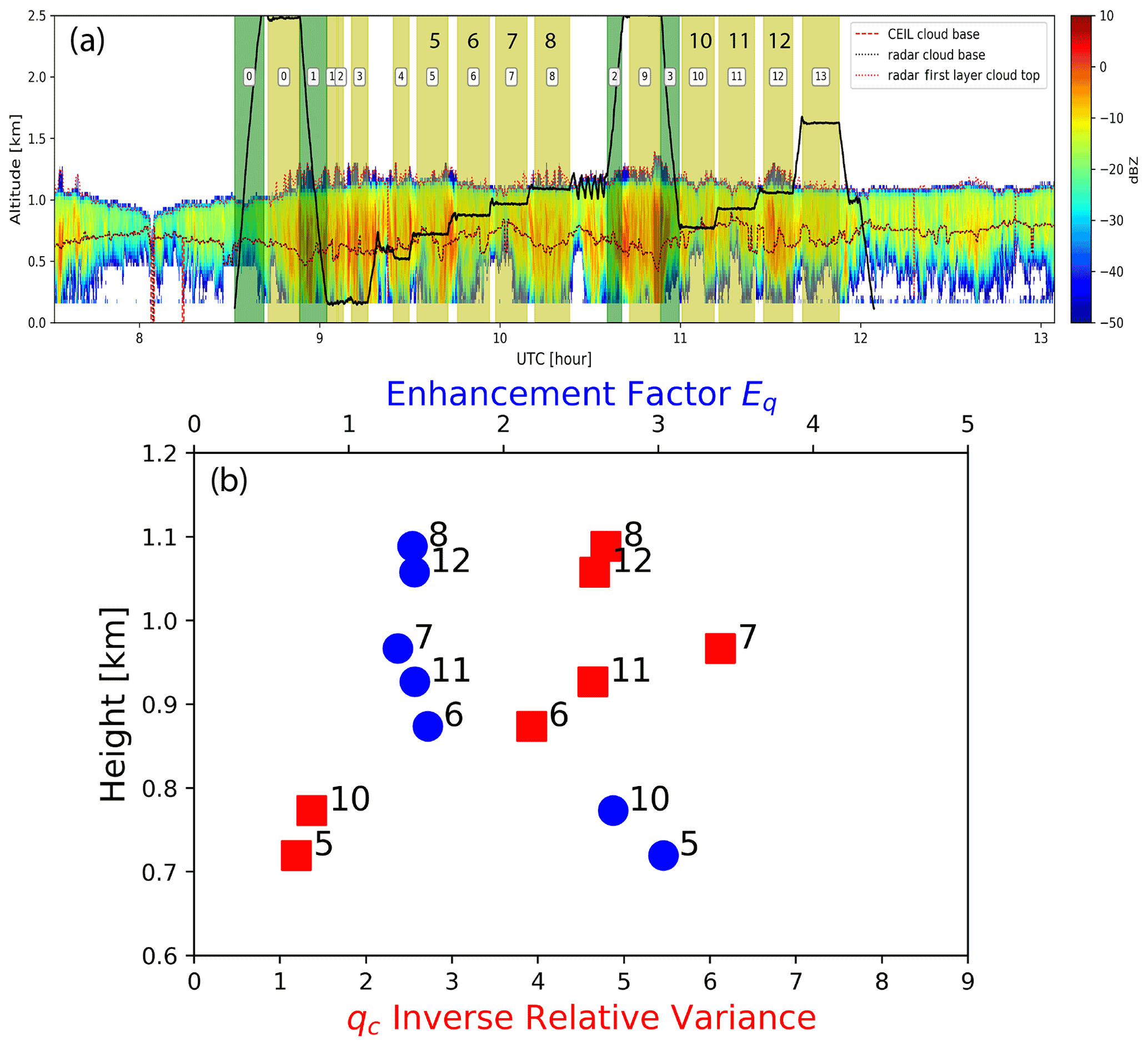
Figure 1 (a) The vertical flight track of the G-1 (thick black line) overlaid on the radar reflectivity contour by the ground-based KAZR during the 18 July 2017 RF around the DOE ENA site on Graciosa Island. The dotted lines in the figure indicate the cloud base and top retrievals from ground-based radar and ceilometer instruments. The yellow-shaded regions are the “hlegs” identified by the Z21 study, among which seven are selected; see the text for their definitions. The figure is adapted from Fig. 1 of Zhang et al. (2021). Panel (b) shows the IRV ${\mathit{\nu }}_{q_{\mathrm{c}}}$ (red squares) and enhancement factor E (blue circles) as a function of height that are derived from the selected hlegs 5, 6, 7, 8, 10, 11, and 12 in panel (a). Note that the lower x axis range differs from that in Fig. 4c of Zhang et al. (2021), as their IRV is calculated as the mean divided by standard deviation (see their caption), whereas we show the mean squared divided by the variance.

Figure 1b shows the vertical dependence of the inverse relative variance (IRV) of q_c calculated from the seven selected hlegs. Details of how q_c and N_c are calculated from the particle probe data can be found in Zhang et al. (2019). The IRV ${\mathit{\nu }}_{q_{\mathrm{c}}}$ is defined as follows:

$$\begin{array}{}\text{(2)}& {\mathit{\nu }}_{q_{\mathrm{c}}}={\displaystyle \frac{\langle q_{\mathrm{c}}{\rangle }^{\mathrm{2}}}{\mathrm{Var}\left(q_{\mathrm{c}}\right)}},\end{array}$$

where 〈q_c〉 and Var(q_c) are the mean and variance of q_c, respectively. As such, the IRV can be considered as an index of cloud water horizontal homogeneity, where a more homogeneous cloud water field will have a larger value of IRV. As shown in Fig. 1b, the value of ${\mathit{\nu }}_{q_{\mathrm{c}}}$ is only about 1.0–1.25 at cloud base (i.e., hlegs 5 and 10). It first increases upward for the hlegs in the center of the cloud (i.e., hlegs 6, 7, and 11) and peaks at about 1 km for hleg 7. Interestingly, the value of ${\mathit{\nu }}_{q_{\mathrm{c}}}$ for the two cloud-top hlegs (8 and 12) becomes smaller than that of hleg 7. E is defined as $E=<f\left(q_{\mathrm{c}}\right)>/f(<q_{\mathrm{c}}>)$, where f is the autoconversion function. As the value of E for autoconversion due to q_c variation is inversely proportional to ${\mathit{\nu }}_{q_{\mathrm{c}}}$, E first decreases from cloud base upward before reaching a minimum around 1 km (i.e., hleg 7) and then increasing slightly toward cloud top. This result indicates that the enhancement factor is vertically dependent and should not simply be treated as a constant. Our simulations aim to provide insights into the mechanisms governing the vertical dependence of E_q.

3 LES model description and configuration

The LES model used in this study is the System for Atmospheric Modeling (SAM v6.10.6;  Khairoutdinov and Randall, 2003). SAM is based on a nonhydrostatic and anelastic equation set. The momentum variables use second-order centered spatial differences and third-order Adams–Bashforth time differencing. Scalar advection uses a fifth-order advection scheme (ULTIMATE–MACHO; Yamaguchi et al., 2011), which minimizes artificial numerical diffusion across the inversion. Subgrid-scale fluxes are formulated using the 1.5-order approach of Deardorff (1980). Horizontal boundary conditions are doubly periodic. The upper boundary is a rigid lid with Rayleigh damping applied to the upper one-third of the domain to minimize reflection of internal gravity waves off the top boundary.

The control simulation employs a domain size of 30.24 × 30.24 × 20 km³ (864 × 864 × 192 grid points), a horizontal scale roughly similar to the seven selected hlegs in Z21. All additional sensitivity simulations employ a smaller domain size of 8.96 × 8.96 × 20 km³ (256 × 256 × 192 grid points). The horizontal grid spacing is 35 m, while the vertical grid spacing is 5 m near the surface and inversion layer, increasing to near 1500 m at the top of the domain. The deep domain is required to accurately calculate the downwelling radiation streams at cloud level. Shortwave and longwave fluxes are calculated using the radiation parameterization adapted from the National Center for Atmospheric Research (NCAR) Community Climate Model (CCM3; Kiehl et al., 1998).

Microphysical processes are represented using a simplified version of the Khairoutdinov and Kogan (2000) parameterization. Similar to the classic Kessler parameterization (Kessler, 1969), the Khairoutdinov and Kogan (2000) parameterization is based on partial moments of the drop size distribution. As originally formulated, it is a fully interactive, two-moment parameterization that includes conservation equations for mass and number concentration of both cloud (i.e., q_c and N_c) and rain (i.e., q_r and N_r, where the subscript “r” indicates rain) species. In this study, the parameterization is simplified somewhat by holding the droplet concentration fixed at a user-specified value. In this approach, specifying the N_c is a proxy for the cloud concentration nuclei (CCN) concentration. Our control simulation uses a value of N_c=75 cm⁻³, which is based on airborne in situ measurements of the 18 July 2017 case (Zhang et al., 2021). In addition to the control simulation, several model sensitivity runs are performed to characterize the impacts of varying N_c between 50 and 100 cm⁻³ (see Sect. 4.4). For reasons of computational expense, these sensitivity simulations are run over smaller domains of 256 × 256 × 192. Fixing the N_c value allows us to isolate how the variability in liquid water influences microphysical process rates. Future studies will include interactive N_c values to explore the mutual influence of the variability of liquid water and droplet concentration on process rates.

Model initial conditions are based on the 11:38 UTC sounding from Graciosa Island, roughly coinciding with the G-1 flight and our main analysis interval from 09:00 to 12:00 UTC. The soundings before and after the 11:38 UTC soundings indicate a deepening of the boundary layer followed by a reduction of depth (Fig. 2). The initial LES mean profiles are constructed from simple piecewise approximations to the sounding profiles. Mixed-layer θ_l and q_t are 292.2 K and 11.2 g kg⁻¹, respectively, with jumps across the inversion of ∼ 7 K and ∼ –3 g kg⁻¹. The height of the inversion in the LES initial conditions is 1132.5 m (895 hPa).

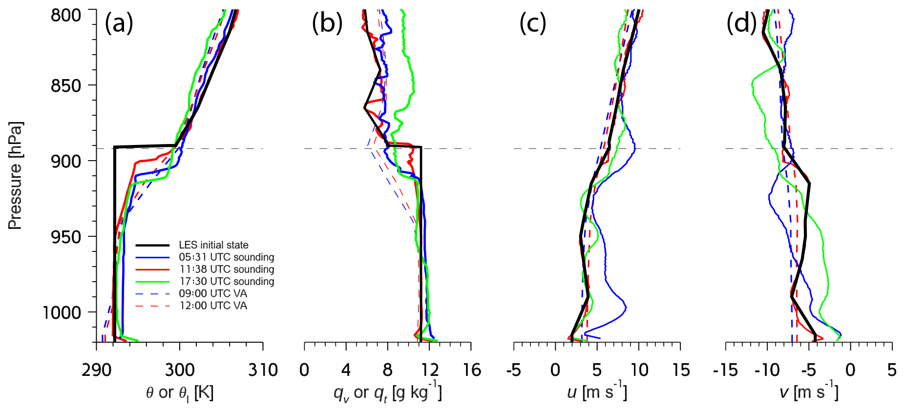
Figure 2 Vertical profiles of the 18 July 2017 boundary layer from radiosondes taken at Graciosa Island (05:81, 11:38, and 17:30 UTC) and the ARM VARANAL product (09:00 and 12:00 UTC), which itself assimilates the soundings. The figure panels show the following: (a) potential temperature or liquid water potential temperature (LES profile), (b) water vapor mixing ratio or total water mixing ratio (LES profile), (c) u, and (d) v. The solid black line represents the simplified LES initial condition profile constructed from the 11:38 UTC sounding.

Model simulations run from 06:00 to 15:00 UTC for 18 July 2017. Large-scale vertical velocity and advective tendencies of temperature and moisture are provided from the 3-hourly DOE ARM variational analysis product (VARANAL; Zhang and Lin, 1997; Xie et al., 2014) and are shown in Fig. 3. The simulation period is characterized by cold advection throughout the depth of the troposphere. Drying at low levels is overlaid by a layer that is drying from 03:00 to 09:00 UTC and then moistening from then onward. The vertical motion field is dominated by subsidence. Although we could calculate fluxes interactively based on the observed sea surface temperature of 294.9 K, we choose to impose surface fluxes taken from the VARANAL product. The fluxes are time-varying but have mean values of 11.8 W m⁻² (sensible) and 105.8 W m⁻² (latent) over the simulation period. The surface stress is a constant imposed value of 0.0625 m² s⁻². SAM configuration files are located at https://github.com/dmechem/ENA_variability_LES_bulk_paper (last access: 28 October 2021).

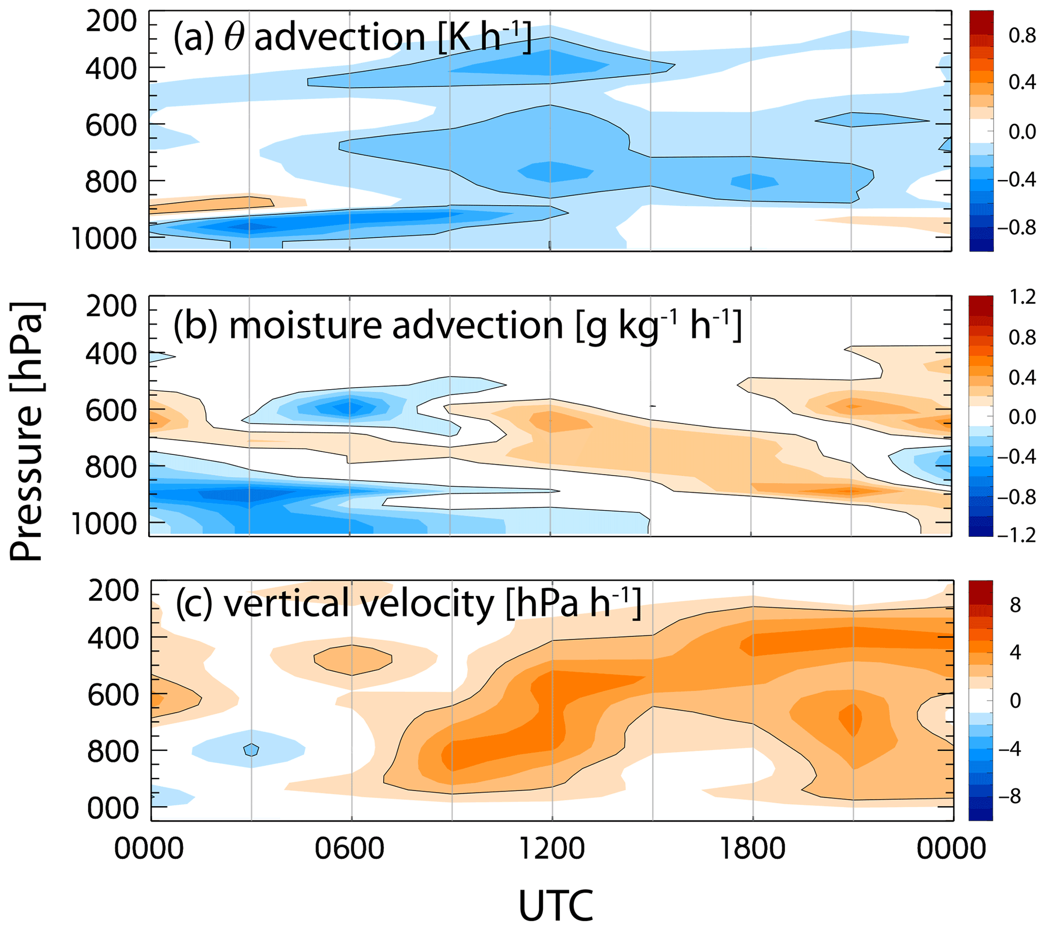
Figure 3 Time–height sections of potential temperature and moisture advection, and large-scale vertical velocity taken from the ARM VARANAL product. The simulation period is from 06:00 to 15:00 UTC.

4 Results

4.1 LES base state and mean turbulent fluxes

The mean control-simulation profiles in Fig. 4, taken over the averaging period from 09:00 to 12:00 UTC, show that stratocumulus clouds dominate the domain. We define cloud as points having a liquid cloud water mixing ratio (q_c) of 0.01 g kg⁻¹ or greater. The main stratocumulus cloud layer extends from an average cloud-base height of 821 m to an average cloud-top height of 1109 m (Fig. 4a). The cloud boundaries agree well with the in situ and ground measurements in Z21 (see their Figs. 1 and 4). The PDF of cloud-base heights in Fig. 4e shows the prevalent stratocumulus cloud base and a secondary peak corresponding to shallow cumulus, most of which rise into the stratocumulus deck. Mean cloud base and cloud top are denoted by the lower and upper gray lines, respectively. The cloud fraction is 0.5 at these levels (Fig. 4d), with a fully cloudy domain occurring between 900 and 1050 m. The liquid water and cloud fraction profiles (Fig. 4a and d, respectively) indicate the presence of cumulus occurring below the main stratocumulus deck. These cumulus extend down to 450 m and are characterized by a lower area fraction (∼ 0.1); therefore, they only contribute a small amount to the mean q_c profile. The stratocumulus deck is characterized by a nearly linear increase in q_c from the mean cloud base upward, peaking at ∼ 0.5 g kg⁻¹ close to the mean cloud top. Liquid water variance increases only slowly with height from the mean cloud base up to a height of approximately 1.04 km, above which it rapidly increases, reflective of the effects of entrainment. Variables q_t and θ_l are weakly stratified in the subcloud layer but are relatively constant (10.5 g kg⁻¹ and 292 K, respectively) from 700 m upward to within a few tens of meters of the top of the cloud (Fig. 4b and c, respectively). Variance of q_t and θ_l is small over the bulk of the boundary layer, only increasing from entrainment near the upper part of the cloud similar to the q_c variance.

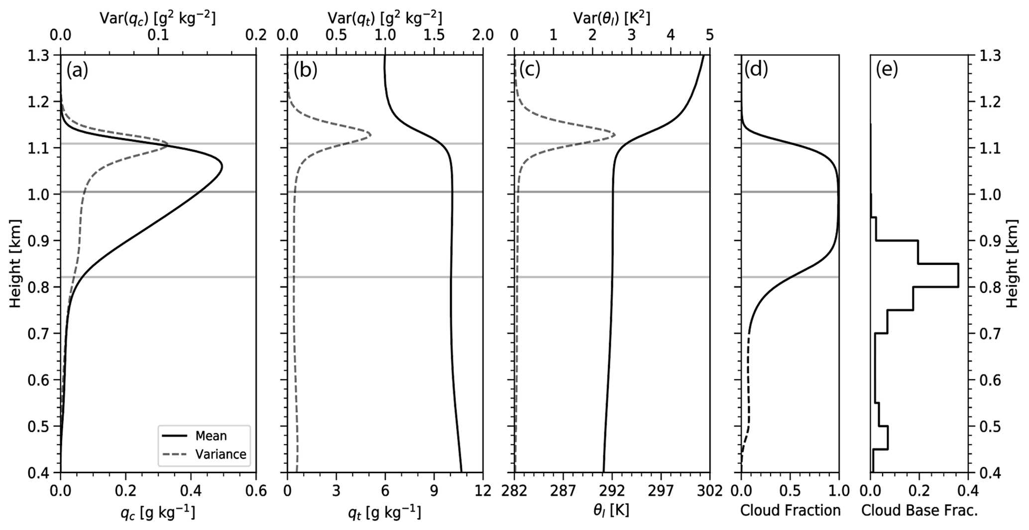
Figure 4 Vertical profile of the horizontal average (mean) and variance, over the analysis period of 09:00–12:00 UTC, of (a) the cloud liquid water mixing ratio q_c, (b) the total water q_t, (c) the liquid water potential temperature θ_l, and (d) the cloud area fraction. The solid lines indicate mean quantities, and the dashed lines indicate variance. From bottom to top, the gray lines indicate the mean cloud base, the bottom boundary of the entrainment zone, and the mean cloud top, respectively. (e) Histogram of cloud-base height, with each value representing the area fraction of cloud bases lying within that 50 m height interval.

Buoyancy flux slowly increases in the stratocumulus layer, peaking near 20 W m⁻² in the upper half of the cloud, as shown in Fig. 5a. Entrainment at cloud top is manifested by negative values of buoyancy flux ($w^{\prime }{\mathit{\theta }}_{\mathrm{v}}^{\prime }<\mathrm{0}$, i.e., entrainment acting to transport warm air downward). Below the main stratocumulus layer, the buoyancy flux shows signs of decoupling in the subcloud layer. This arises due to the evaporative cooling from rain that creates a stable layer below the stratocumulus, requiring the turbulence to do work against the stable stratification in an attempt to homogenize the layer. This stratification also helps to explain some of the rising cumulus below the main stratocumulus deck, as the decoupling leads to a buildup of conditional instability in the mixed layer to support cumulus growth.

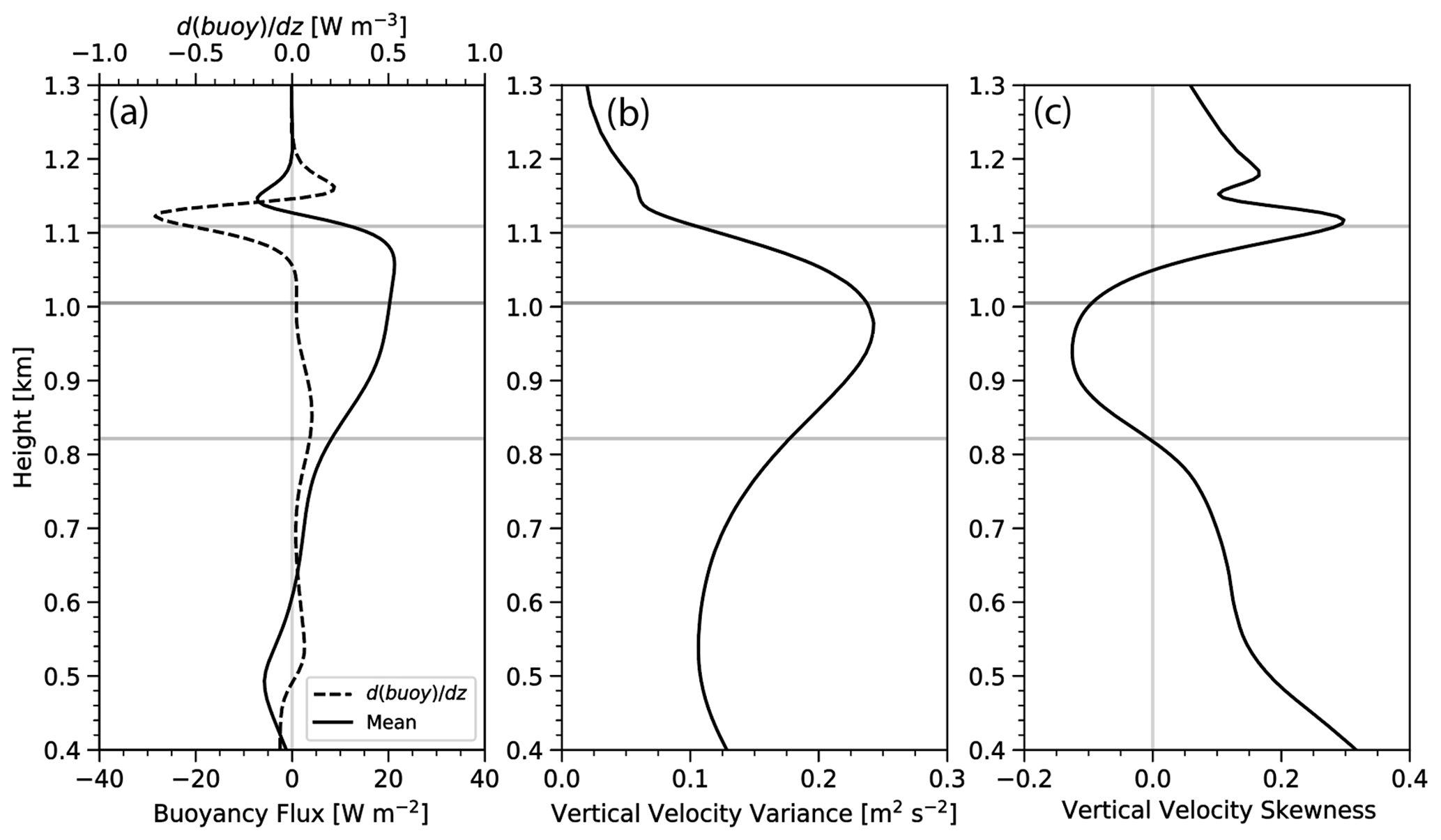
Figure 5 Vertical profiles of the horizontally averaged (a) buoyancy flux, (b) vertical velocity variance, and (c) vertical velocity skewness. The dashed line in panel (a) represents the first derivative of the buoyancy flux. The gray lines are as in Fig. 4.

We use the buoyancy flux to diagnose the depth of the entrainment zone. Although we recognize that the effects of cloud-top entrainment are undeniably, over time, communicated throughout the boundary layer, we define the entrainment zone to be the depth to which the entraining free troposphere initially penetrates. We define this as the depth at which the profile of the buoyancy flux switches direction (i.e., where the derivative of the buoyancy flux is zero). Figure 5a shows that the gray line at 1.005 km denoting the bottom of the entrainment zone (also overlaid on all the panels of Figs. 4 and 5) coincides with the maximum of the buoyancy flux and the zero of the derivative of the buoyancy flux. At this level, the variances of q_c, q_t, and θ_l begin to increase substantially.

Vertical velocity variance (Fig. 5b) begins to increase in the cumulus layer and peaks within the upper stratocumulus layer, consistent with increasing buoyancy production. Positive vertical velocity skewness (Fig. 5c) occurs in the cumulus region in a manner consistent with other studies showing cumulus (narrow, strong updrafts, and broad, weaker downdrafts) rising into stratocumulus (Stevens et al., 2001). Skewness over the bulk of the stratocumulus cloud is predominantly negative (narrow, strong downdrafts and broad, weak updrafts), which is consistent with observations of radiatively driven stratocumulus (e.g., Stevens et al., 2003). The increase of skewness near cloud top is associated with entrainment and is ubiquitous in stratocumulus simulations.

Figure 6 shows a snapshot plan view of the liquid water path (LWP) over the domain taken at 10:30 UTC. The LWP is highly variable, with maxima over 300 g m⁻² and minima below 25 g m⁻². Two arbitrarily selected vertical cross sections of cloud and rainwater mixing ratio show that LWP variability often corresponds to variability in cloud depth. Cloud-base height is much more variable than cloud-top height, which is typical of stratocumulus whose tops are constrained by a strong inversion. The vertical slices also show indications of cumulus rising into stratocumulus (Fig. 6c, between 21.5 and 22.0 km). Regions of rainwater mixing ratio in Fig. 6b and c are, broadly speaking, confined to regions of cloud with higher LWP and cloud water mixing ratio.

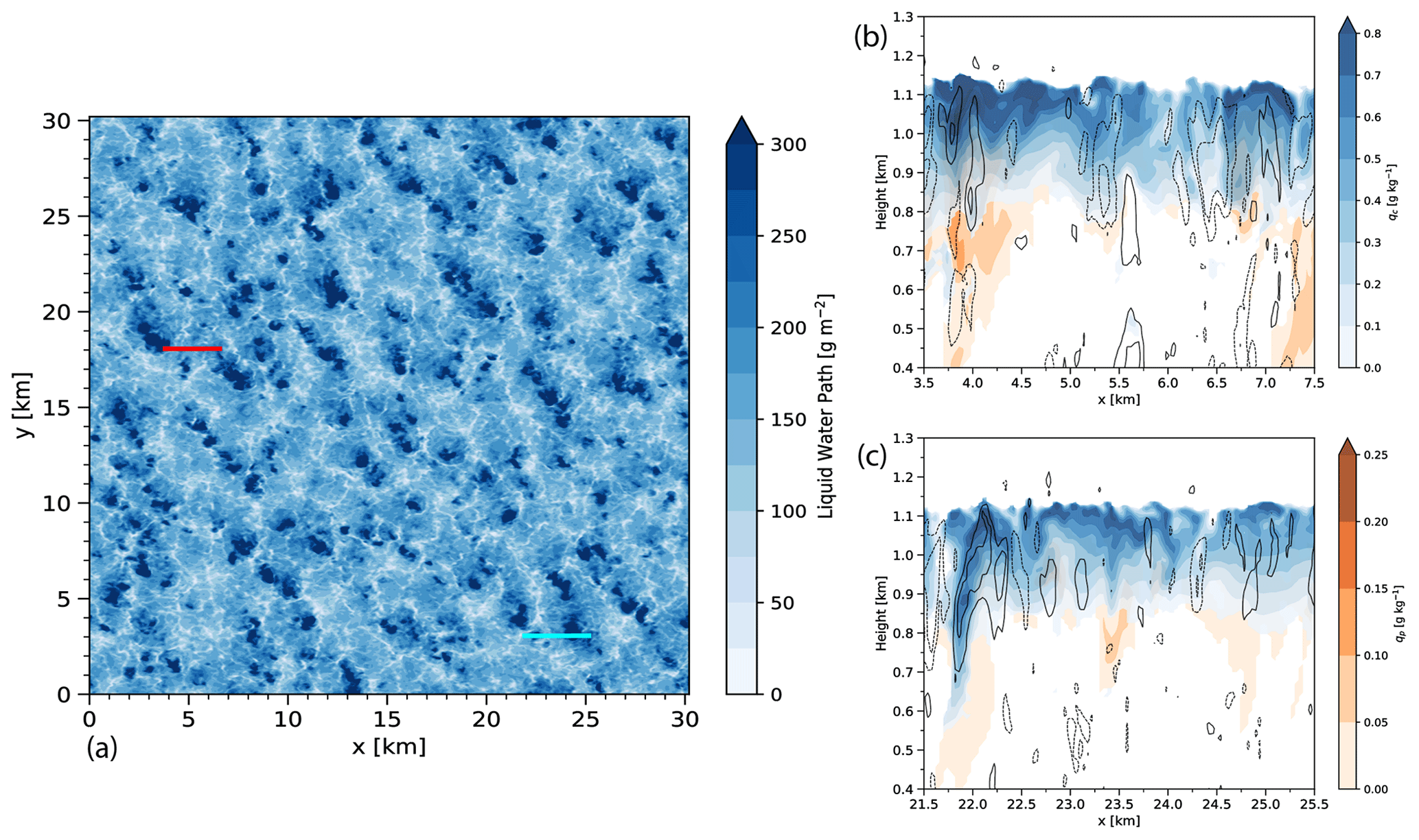
Figure 6 (a) Plan view of the cloud liquid water path. Panels (b) and (c) correspond to vertical cross sections of the cloud water mixing ratio (q_c, blue), the rainwater mixing ratio (q_r, orange), and contours of vertical velocity w. w is contoured every 0.5 m s⁻¹, with the solid lines representing positive values and the dashed lines representing negative values. The red and blue lines in panel (a) correspond to the locations of the vertical cross sections in panels (b) and (c), respectively.

4.2 Vertical profiles of cloud horizontal variability

We quantify the horizontal variability of the q_c using its IRV ${\mathit{\nu }}_{q_{\mathrm{c}}}$ defined in Eq. (2). As mentioned earlier, the larger the value of ${\mathit{\nu }}_{q_{\mathrm{c}}}$, the smaller the horizontal variation of q_c in relation to the mean. The vertical profile of ${\mathit{\nu }}_{q_{\mathrm{c}}}$ in Fig. 7a increases upward from the base of the stratocumulus layer (the dashed lines at z=821 m), peaking just above the lower extent of the entrainment zone near 1020 m and then sharply decreasing up to cloud top. The shape of this profile agrees well with the aircraft observations from Zhang et al. (2021) overplotted on Fig. 7a, which also exhibit an increase in ${\mathit{\nu }}_{q_{\mathrm{c}}}$ throughout the cloud layer and then decrease closer to cloud top (see also Fig. 1b).

The portion of the profiles between the mean cumulus and stratocumulus cloud bases (i.e., between 475 and 821 m) exhibits a decrease in ${\mathit{\nu }}_{q_{\mathrm{c}}}$ corresponding to an increase in relative variability. The mean q_c throughout the layer is increasing (a consequence of the increase of q_c with height from condensation) just as in stratocumulus. The increase in standard deviation with height is likely a consequence of the cloud-top distribution of the cumulus, specifically, that not all the cumulus rise completely into the stratocumulus deck. Keeping in mind that these calculations are conditioned on cloudy points at each level, this variability in cloud-top height over the cumulus layer means fewer cloud samples with height, leading to larger values of standard deviation.

Breaking down ${\mathit{\nu }}_{q_{\mathrm{c}}}$ into its constituent mean and standard deviation values (Fig. 7a) demonstrates that the increase in ${\mathit{\nu }}_{q_{\mathrm{c}}}$ throughout the lower two-thirds of the stratocumulus cloud layer is largely not due to changes in horizontal variability but rather mainly because of the adiabatic increase of mean q_c (i.e., the numerator term in Eq. 2). The standard deviation of q_c varies little over this portion of the cloud layer. In the entrainment zone, the variability of q_c begins to increase with height, while the mean q_c increases more slowly with height. The behavior of the q_c mean and variability are both likely effects of cloud-top entrainment, which, combined together, yields the sharp decrease in ${\mathit{\nu }}_{q_{\mathrm{c}}}$.

To achieve a quantitative understanding of the relative roles of the mean and standard deviation in determining how ${\mathit{\nu }}_{q_{\mathrm{c}}}$ changes with height, we use the chain rule to take the derivative of ${\mathit{\nu }}_{q_{\mathrm{c}}}$ with respect to height z:

$$\begin{array}{}\text{(3)}& \begin{array}{rl}{\displaystyle \frac{\mathrm{d}{\mathit{\nu }}_{q_{\mathrm{c}}}}{\mathrm{d}z}}& ={\displaystyle \frac{\mathrm{d}}{\mathrm{d}z}}\left({\displaystyle \frac{\langle q_{\mathrm{c}}{\rangle }^{\mathrm{2}}}{\mathrm{Var}\left(q_{\mathrm{c}}\right)}}\right)\\ & =\underset{\text{Term 1}}{\underbrace{{\displaystyle \frac{\mathrm{2}\langle q_{\mathrm{c}}\rangle }{\mathrm{Var}\left(q_{\mathrm{c}}\right)}}{\displaystyle \frac{\mathrm{d}\langle q_{\mathrm{c}}\rangle }{\mathrm{d}z}}}}\underset{\text{Term 2}}{\underbrace{-{\displaystyle \frac{\langle q_{\mathrm{c}}{\rangle }^{\mathrm{2}}}{{\mathrm{Var}}^{\mathrm{2}}\left(q_{\mathrm{c}}\right)}}{\displaystyle \frac{\mathrm{dVar}\left(q_{\mathrm{c}}\right)}{\mathrm{d}z}}}},\end{array}\end{array}$$

where the first term on the right-hand side (Term 1) reflects the impact of the vertical variation of mean q_c, and the second term (Term 2) reflects the impact of the vertical variation of variance of q_c. In the cumulus layer, changes with height of both mean and variance of q_c contribute to the variation with height of ${\mathit{\nu }}_{q_{\mathrm{c}}}$, as shown in Fig. 7b. Term 1 is greater near mean cumulus cloud base, contributing to a positive $\mathrm{d}{\mathit{\nu }}_{q_{\mathrm{c}}}/\mathrm{d}z$. Above this maximum, a negative maximum in Term 2 is associated with $\mathrm{d}{\mathit{\nu }}_{q_{\mathrm{c}}}/\mathrm{d}z$ becoming negative. In the lower part of the stratocumulus layer, an increasingly positive Term 1 dominates the change in variability of ${\mathit{\nu }}_{q_{\mathrm{c}}}$, while Term 2 (and, thus, the impact of the variance of q_c) is small and then becomes more negative approaching the base of the entrainment zone. At this point, Term 1 remains positive but begins to decrease as adiabatic mean q_c growth slows, but Term 2 becomes increasingly negative due to increased q_c variance variability from the effects of cloud-top entrainment. Beginning about 20 m above the base of the entrainment zone, $\mathrm{d}{\mathit{\nu }}_{q_{\mathrm{c}}}/\mathrm{d}z$ becomes negative up to cloud top as Term 2 remains the dominant term from entrainment and Term  1 (which is decreasing with height) becomes less important.

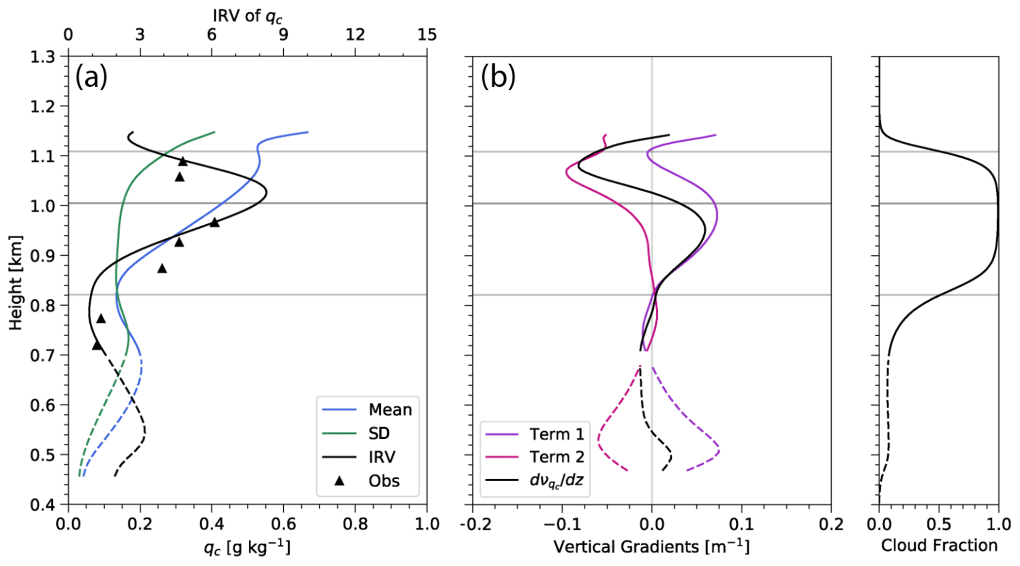
Figure 7 Vertical profiles of the horizontally averaged (a) mean, standard deviation, and inverse variance of q_c and (b) the derivatives of the inverse variance of q_c. The dashed lines represent the cumulus cloud layer. Triangle markers represent the inverse variance of observed q_c. Term 1 and Term 2 are calculated as defined in Eq. (3). The gray lines are as in Fig. 3.

The above analysis clearly demonstrated the advantages and usefulness of LES in comparison with in situ observations. First of all, the thermodynamic structure of MBL and stratocumulus cloud from the LES shed important light on the underlying physical processes (i.e., condensation and entrainment) that influence the cloud vertical structure and horizontal variation. Second, the LES better resolves the vertical structure of the cloud field, which allows us to perform the decomposition analysis as in Fig. 7 to obtain a more confident and comprehensive understanding of the vertical dependence of q_c horizontal variability.

4.3 Vertical profiles of enhancement factor

In the single-moment microphysical parameterization used in these simulations, the enhancement factor E_q can be formulated as in Zhang et al. (2019) to be

$$\begin{array}{}\text{(4)}& E_q={\displaystyle \frac{{\int }_{\mathrm{0}}^{\mathrm{\infty }}{q}_{\mathrm{c}}^{{\mathit{\beta }}_q}P\left(q_{\mathrm{c}}\right)\mathrm{d}{q}_{\mathrm{c}}}{\langle q_{\mathrm{c}}{\rangle }^{{\mathit{\beta }}_q}}},\end{array}$$

where P(q_c) represents the probability density function of q_c. Because we hold N_c constant in this study, we consider only the variability in cloud water in formulating E_q. In the cumulus region, E_q varies between 1 and 2 and slowly increases with height approaching the mean stratocumulus base, peaking at 3.80 near 800 m (Fig. 8a). Above cloud base, E_q sharply decreases to approximately 1 in the upper one-third of the stratocumulus layer. In the entrainment zone, E_q begins to slightly increase and approaches 2 above mean cloud top. Model calculations of E_q are similar to those calculated from aircraft observations from the Z1 case (Zhang et al., 2021), both over the stratocumulus layer itself and just below the mean stratocumulus cloud base. Aircraft observations overlaid on Fig. 8a correlate well with calculated E_q, agreeing with the idea of a decreasing E_q profile throughout the cloud layer. The previous analysis of ${\mathit{\nu }}_{q_{\mathrm{c}}}$ suggests that the large vertical variations of E_q in the stratocumulus layer are predominantly due to adiabatic increase of mean q_c, whereas the impact of q_c variances are more minimal until closer to cloud top.

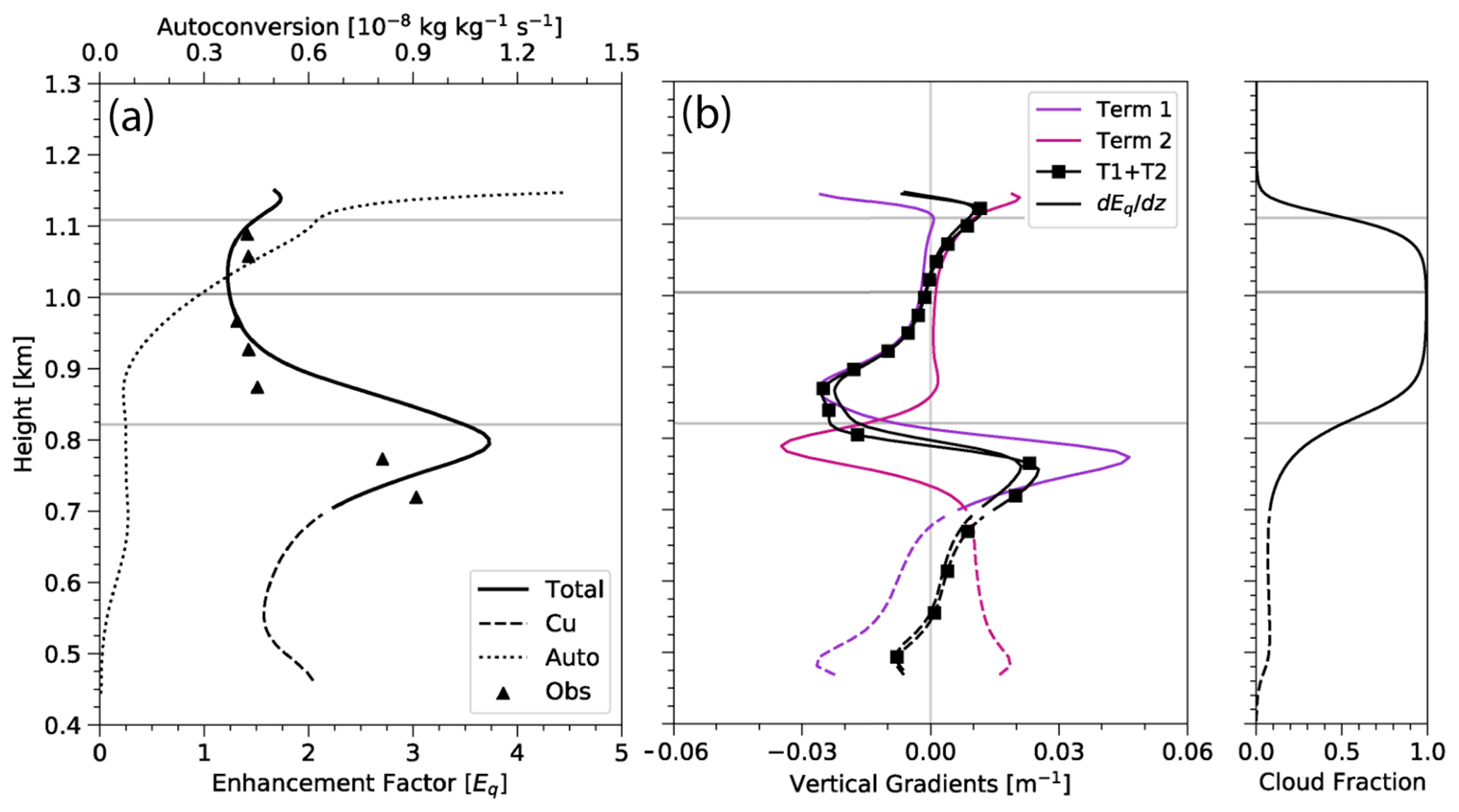
Figure 8 Vertical profiles of the horizontally averaged (a) enhancement factor E_q and autoconversion and (b) the derivatives of the enhancement factor E_q. As in Fig. 7, the dashed lines represent the cumulus cloud layer. Term 1 and Term 2 are calculated as defined in Eq. (3). The gray lines are as in Fig. 4.

Figure 8a includes a vertical profile of mean autoconversion to provide context to the relevance of E_q in the precipitation process. E_q is large (>3) near cloud base where the liquid water content (and, hence, autoconversion) is very small. The values of E_q are much more modest (i.e., 1–2) over the portion of the cloud where autoconversion is larger and the precipitation process is more active. This is a subtle point but may be important when it is desirable to distill the E_q profile down to a single representative value, as an average value of E_q should be weighted in such a way to provide a representative enhancement factor in situations relevant for precipitation formation. In this case, weighting E_q at each level by autoconversion may yield the most representative single value of E_q.

A lognormal distribution has been shown to represent observations of q_c well (e.g., Lebsock et al., 2013; Zhang et al., 2019), so we represent E_q in terms of the parameters of a lognormal distribution as in Zhang et al. (2021):

$$\begin{array}{}\text{(5)}& E_q\left({\mathit{\nu }}_{q_{\mathrm{c}}},{\mathit{\beta }}_{q_{\mathrm{c}}}\right)=(\mathrm{1}+{\displaystyle \frac{\mathrm{1}}{{\mathit{\nu }}_{q_{\mathrm{c}}}}}{)}^{\frac{{\mathit{\beta }}_{q_{\mathrm{c}}}^{\mathrm{2}}-{\mathit{\beta }}_{q_{\mathrm{c}}}}{\mathrm{2}}},\end{array}$$

where E_q represents the enhancement factor related solely to variability in q_c. Equation (5) nicely demonstrates the dependence of E_q on the inverse relative variance. In particular, Eq. (5) shows that a PDF of q_c undergoing adiabatic ascent and shifting toward larger values of q_c but maintaining its variance will exhibit larger mean values of q_c, thus causing an increase of ${\mathit{\nu }}_{q_{\mathrm{c}}}$ and a reduction of $E_{q_{\mathrm{c}}}$. Stated differently, E_q depends on the relative variance not the variance itself.

Using this definition of E_q based on the lognormal assumption of the q_c distribution, we can differentiate it with respect to height to explore the association between vertical gradients in E_q and vertical profiles of mean and standard deviation of q_c:

$$\begin{array}{}\text{(6)}& \begin{array}{rl}{\displaystyle \frac{\mathrm{d}{E}_q}{\mathrm{d}z}}& ={\displaystyle \frac{\mathrm{d}}{\mathrm{d}z}}(\mathrm{1}+{\displaystyle \frac{\mathrm{1}}{{\mathit{\nu }}_{q_{\mathrm{c}}}}}{)}^{\mathit{\gamma }}\\ & =\mathit{\gamma }{\left(\mathrm{1}+{\displaystyle \frac{\mathrm{1}}{\mathit{\nu }}}\right)}^{\mathit{\gamma }-\mathrm{1}}\left({\displaystyle \frac{-\mathrm{1}}{{\mathit{\nu }}_{q_{\mathrm{c}}}^{\mathrm{2}}}}\right){\displaystyle \frac{\mathrm{d}{\mathit{\nu }}_{q_{\mathrm{c}}}}{\mathrm{d}z}},\end{array}\end{array}$$

where $\mathit{\gamma }=({\mathit{\beta }}_{q_{\mathrm{c}}}^{\mathrm{2}}-{\mathit{\beta }}_{q_{\mathrm{c}}})/\mathrm{2}$. Using the expression for $\mathrm{d}{\mathit{\nu }}_{qc}/\mathrm{d}z$ from Eq. (3), we obtain

$$\begin{array}{}\text{(7)}& \begin{array}{rl}{\displaystyle \frac{\mathrm{d}{E}_q}{\mathrm{d}z}}& =-{\displaystyle \frac{\mathit{\gamma }}{{\mathit{\nu }}_{q_{\mathrm{c}}}^{\mathrm{2}}}}{\left(\mathrm{1}+{\displaystyle \frac{\mathrm{1}}{\mathit{\nu }}}\right)}^{\mathit{\gamma }-\mathrm{1}}\\ & ({\displaystyle \frac{\mathrm{2}\langle q_{\mathrm{c}}\rangle }{\mathrm{Var}\left(q_{\mathrm{c}}\right)}}{\displaystyle \frac{\partial \langle q_{\mathrm{c}}\rangle }{\partial z}}-{\displaystyle \frac{\langle q_{\mathrm{c}}{\rangle }^{\mathrm{2}}}{{\mathrm{Var}}^{\mathrm{2}}\left(q_{\mathrm{c}}\right)}}{\displaystyle \frac{\partial \mathrm{Var}\left(q_{\mathrm{c}}\right)}{\partial z}})\\ & =\underset{\text{Term 1}}{\underbrace{-C{\displaystyle \frac{\mathrm{2}\langle q_{\mathrm{c}}\rangle }{\mathrm{Var}\left(q_{\mathrm{c}}\right)}}{\displaystyle \frac{\partial \langle q_{\mathrm{c}}\rangle }{\partial z}}}}+\underset{\text{Term 2}}{\underbrace{C{\displaystyle \frac{\langle q_{\mathrm{c}}{\rangle }^{\mathrm{2}}}{{\mathrm{Var}}^{\mathrm{2}}\left(q_{\mathrm{c}}\right)}}{\displaystyle \frac{\partial \mathrm{Var}\left(q_{\mathrm{c}}\right)}{\partial z}}}}\end{array}\end{array}$$

for the decomposition of the vertical gradient of E_q. In Eq. (7), C is defined as follows, without the negative sign:

$$C={\displaystyle \frac{\mathit{\gamma }}{{\mathit{\nu }}_{q_{\mathrm{c}}}^{\mathrm{2}}}}{\left(\mathrm{1}+{\displaystyle \frac{\mathrm{1}}{\mathit{\nu }}}\right)}^{\mathit{\gamma }-\mathrm{1}}.$$

This allows us to utilize a similar analysis to that used to examine the gradient of ${\mathit{\nu }}_{q_{\mathrm{c}}}$ to break down components into impacts from mean q_c and variance of q_c, as shown in Fig. 8. The constant is defined such that an increase in variance with height corresponds to an increase in E_q with height, and an increase in mean q_c with height corresponds to a decrease in E_q with height.

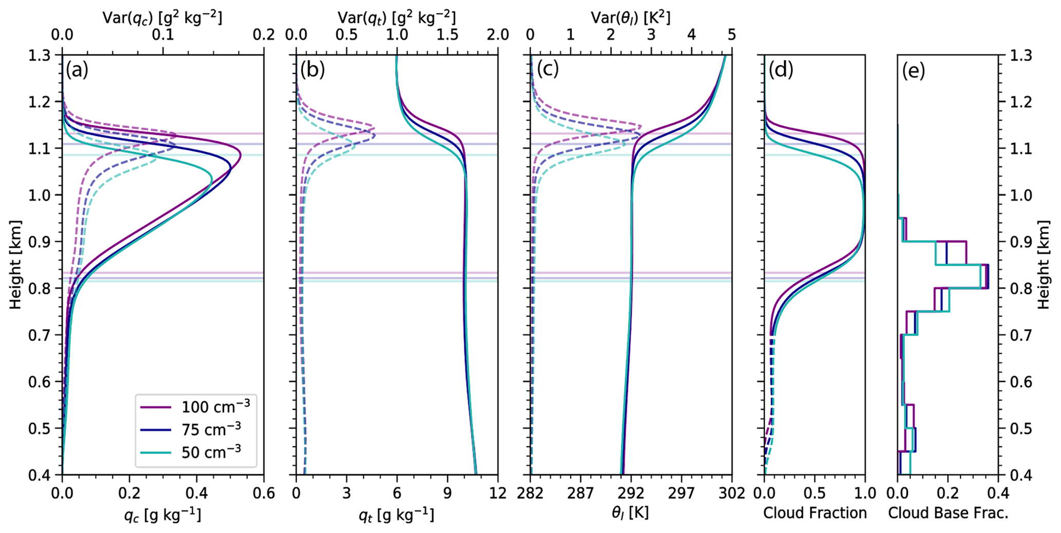
Figure 9 Vertical profile of the horizontal average (mean) and variance, averaged over the analysis period of 09:00–12:00 UTC, of (a) the cloud liquid water mixing ratio q_c, (b) the total water q_t, (c) the liquid water potential temperature θ_l, and (d) the cloud area fraction. The solid lines indicate mean quantities, and the dashed lines indicate variance. (e) Histogram of cloud-base height, with each value representing the area fraction of cloud bases lying within that 50 m height interval. Purple, dark blue, and teal lines represent simulations with N_c values with 100, 75, and 50 cm⁻³, respectively. The colored lines correspond to cloud base and height as in Fig. 4.

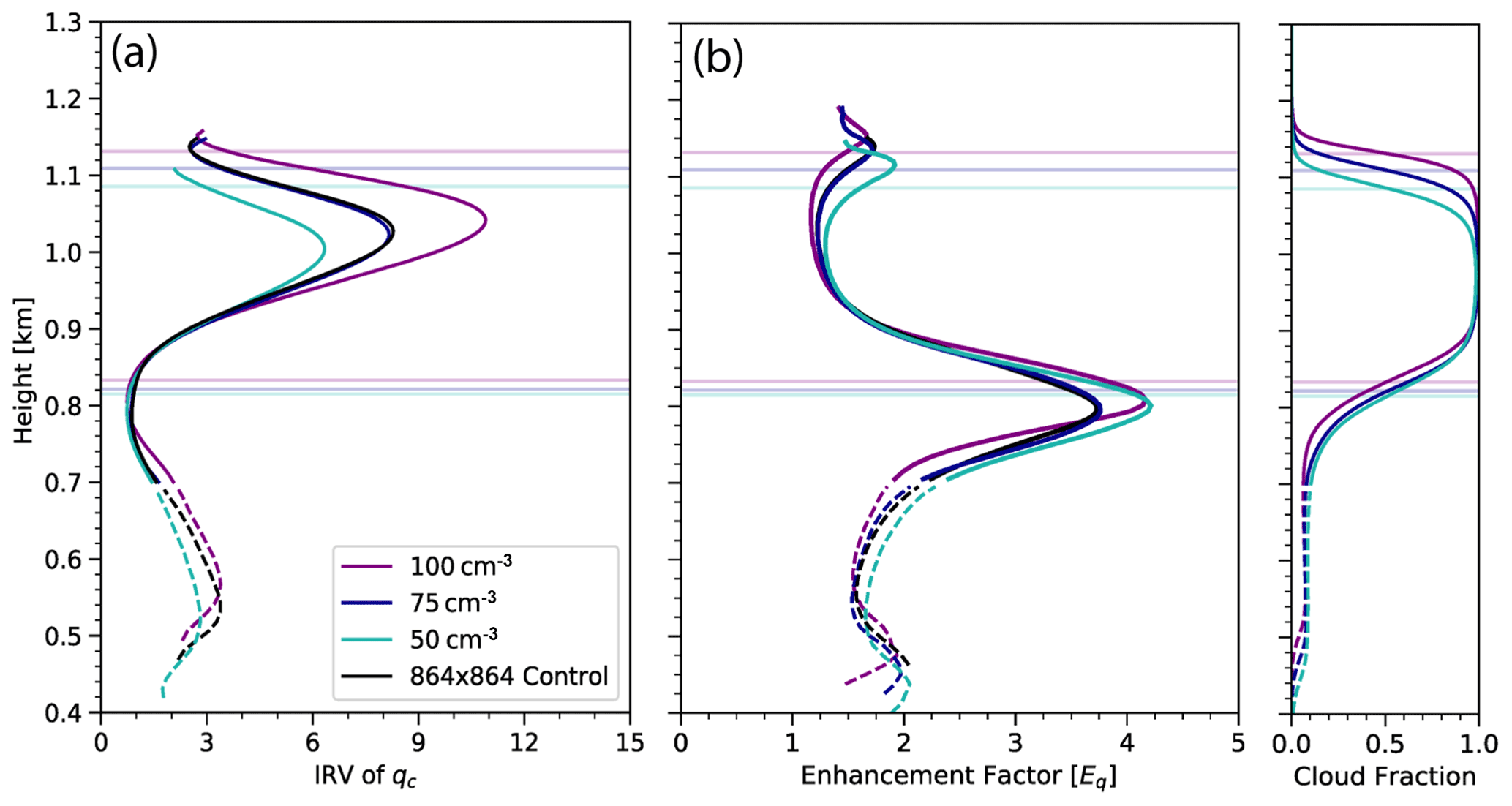
Figure 10 Vertical profiles of the horizontally averaged (a) inverse variance ${\mathit{\nu }}_{q_{\mathrm{c}}}$ and (b) enhancement factor E_q. Solid lines represent total values, whereas dashed lines represent values correlating to only cumulus clouds. Purple, dark blue, and teal lines represent simulations with N_c values of 100, 75, and 50 cm⁻³, respectively, all run over the smaller 256×256 (8.96×8.96 km²) grid. The black lines correspond to the control run using the larger domain and an N_c value of 75 cm⁻³. The colored lines correspond to cloud base and height, as in Fig. 4.

This estimate of $\mathrm{d}{E}_q/\mathrm{d}z$, calculated assuming a lognormal distribution of q_c, matches fairly well to the actual derivative of E_q calculated from the unapproximated PDF (Fig. 8b). Above the cumulus cloud base (∼ 475 m), $\mathrm{d}{E}_q/\mathrm{d}z$ slowly increases as Term 2 remains almost constant but Term 1 approaches zero. Approaching the stratocumulus cloud base at 750 m, $\mathrm{d}{E}_q/\mathrm{d}z$ spikes to near 0.03 m⁻¹ as Term 1 increases but Term 2 decreases to zero. $\mathrm{d}{E}_q/\mathrm{d}z$ then sharply decreases and becomes negative until above the main stratocumulus cloud base, close to 850 m. This is driven by a sharp decrease in Term 1 while Term 2 is also negative but increasing to near zero. Throughout most of the stratocumulus cloud layer, the vertical gradient of E_q is negative due to a negative Term 1 and an almost constantly zero Term 2 but slowly increases to zero. At the base of the entrainment zone, $\mathrm{d}{E}_q/\mathrm{d}z$ becomes zero and then slightly positive as Term 2 becomes more dominant, owing to increased variability of q_c due to entrainment.

Figure 11 Vertical profiles of the horizontally averaged mean, standard deviation, and inverse variance of q_c (same as Fig. 7a) but for four other LES cases from previous studies: (a) DYCOMS-II RF02, (b) ATEX, (c) CAP-MBL, and (d) VOCALS.

4.4 Dependence on droplet concentration

Our simulations use single-moment microphysics where the N_c is specified but is constant throughout the simulation. Smaller droplet concentrations tend to promote precipitation, which should lead to an increase in variability of cloud and precipitation variables. To explore the sensitivity of N_c on the inverse relative variance and enhancement factor, we performed simulations over a range of N_c values. As previously described, these runs employ values of 50 and 100 cm⁻³ to compare to our control simulation of 75 cm⁻³. As previously stated, for reasons of computational expense, we conducted these sensitivity runs (50, 75, and 100 cm⁻³) over smaller domains of 256×256 points (8.96 × 8.96 km²) but plot them alongside the larger-domain control simulation. Mean base state profiles in Fig. 9 show predictable trends across all three sensitivity simulations. Each domain has a cloud fraction of about 0.1 in the cumulus region and a fully cloudy domain in the stratocumulus layer (Fig. 9d). However, cloud bases and cloud heights vary, with mean cloud bases increasing by ∼ 10 m but mean cloud tops increasing by closer to 25 m with each increase in N_c. The decrease in cloud-top height with decreasing N_c likely corresponds to a decrease in entrainment associated with weaker turbulence accompanying the stabilizing effects of increased precipitation (e.g., Stevens et al., 1998). Mean q_c profiles increase similarly, with the deeper clouds associated with larger N_c having greater q_c (Fig. 9a). Profiles of q_t and θ_l are virtually identical from the surface to mean stratocumulus cloud top, where the profiles follow the same trend but again are shifted upward in height by about 30 m with each increase in N_c (Fig. 9b, c). Above the cloud layer (∼ 1200 m), these profiles become identical once again. Variances of q_c and q_t are much closer in value to one another, but each has the same 30 m height increase associated with increasing N_c.

Although main stratocumulus cloud bases differ slightly, the probability density function (PDF) of cloud-base height indicates that a stratocumulus cloud-base height of ∼ 825 m is most common for each N_c sensitivity simulation. The maximum of the PDF is nearly identical for N_c values of 100 and 75 cm⁻³ at 0.36 (Fig. 9e). The 50 cm⁻³ simulation peaks near 825m as well, but it is more of a plateau between 800 and 825 m with a lower probability of 0.26. The PDF also shows a second, smaller peak in cloud-base height in the cumulus region. The cumulus region maximum PDF values are about 0.08, but the corresponding cloud-base values differ slightly across the simulations. The peak frequency occurs near 525 m for a N_c value of 100 cm⁻³, but it is closer to 475 m for the other N_c values.

Further analyzing the impact of the N_c on subgrid-scale variability, we calculate the inverse variance ${\mathit{\nu }}_{q_{\mathrm{c}}}$ and enhancement factor E_q for each N_c simulation. ${\mathit{\nu }}_{q_{\mathrm{c}}}$ is consistent across the different N_c runs with similar features occurring in both the cumulus and stratocumulus cloud layers (Fig. 10a). ${\mathit{\nu }}_{q_{\mathrm{c}}}$ corresponding to N_c of 100 cm⁻³ is the largest among the three simulations. In the stratocumulus layer, the smallest value of N_c (50 cm⁻³) corresponds to the smallest value of ${\mathit{\nu }}_{q_{\mathrm{c}}}$, likely a result of the stabilizing effects of precipitation and the associated reduction in vertical moisture flux from low levels. E_q values for the 3 N_c are even more similar to one another than for ${\mathit{\nu }}_{q_{\mathrm{c}}}$, with some differences near the stratocumulus cloud base (Fig. 10b).

Although not directly accounting for the variability of N_c, this sensitivity study demonstrates that even with varying fixed N_c values, results show consistent trends among key variables. The cloud structure and base states are almost identical, differing slightly in magnitude and shifted in height. An analysis of ${\mathit{\nu }}_{q_{\mathrm{c}}}$ demonstrates similar increasing trends throughout the stratocumulus layer like in the large-domain control simulation. More importantly, E_q shows a clear, almost identical decrease in the stratocumulus layer between cloud base and roughly the beginning of the entrainment zone. Although the differences in ${\mathit{\nu }}_{q_{\mathrm{c}}}$ over the upper part of the cloud are substantial across the simulations, the large values of ${\mathit{\nu }}_{q_{\mathrm{c}}}$ translate only to small differences in small values of E_q. Because of this, the choice of a constant N_c value does not greatly impact the value of E_q.

5 Discussion and conclusions

One of the major uncertainties in warm-rain simulations within ESMs is accounting for microphysical processes occurring at the subgrid scale. Jensen's inequality indicates that neglect of subgrid-scale variability may give rise to biases in nonlinear process rates such as autoconversion, and some current ESMs employ a multiplicative enhancement factor to process rates to crudely account for subgrid-scale variability. In this study, we use LES to explore the behavior of the quantities determining the autoconversion enhancement factor. Our chief findings are as follows:

• Both inverse relative variance ${\mathit{\nu }}_{q_{\mathrm{c}}}$ and enhancement factor E_q vary considerably in the vertical. ${\mathit{\nu }}_{q_{\mathrm{c}}}$ ranges from 0 to nearly 9, while E_q varies from close to 1 to 3.70.

• The profile of inverse relative variance ${\mathit{\nu }}_{q_{\mathrm{c}}}$ throughout most of the stratocumulus and underlying cumulus layers is explained largely by changes to the mean q_c profile, predominantly dictated by adiabatic processes and not by variability in q_c.

• The profile of enhancement factor E_q is largely consistent with that of ${\mathit{\nu }}_{q_{\mathrm{c}}}$ and peaks near cloud base, with a minimum over the upper half of the cloud. E_q is governed by the inverse relative variance and not simply the absolute width of the distribution, so a q_c distribution undergoing only adiabatic ascent will yield a reduction of E_q.

• Over the upper one-third of the stratocumulus layer where entrainment is highly influential, the increased variance of q_c has a substantial effect on ${\mathit{\nu }}_{q_{\mathrm{c}}}$ and E_q.

• Because E_q is so strongly governed by adiabatic (condensational) increase of q_c with height, which is a structural feature of MBL stratocumulus, the shape of our profiles of ${\mathit{\nu }}_{q_{\mathrm{c}}}$ and E_q likely generalize to other cases of high-cloud-fraction stratocumulus.

• Representing the q_c distribution using a lognormal function is a reasonable approximation.

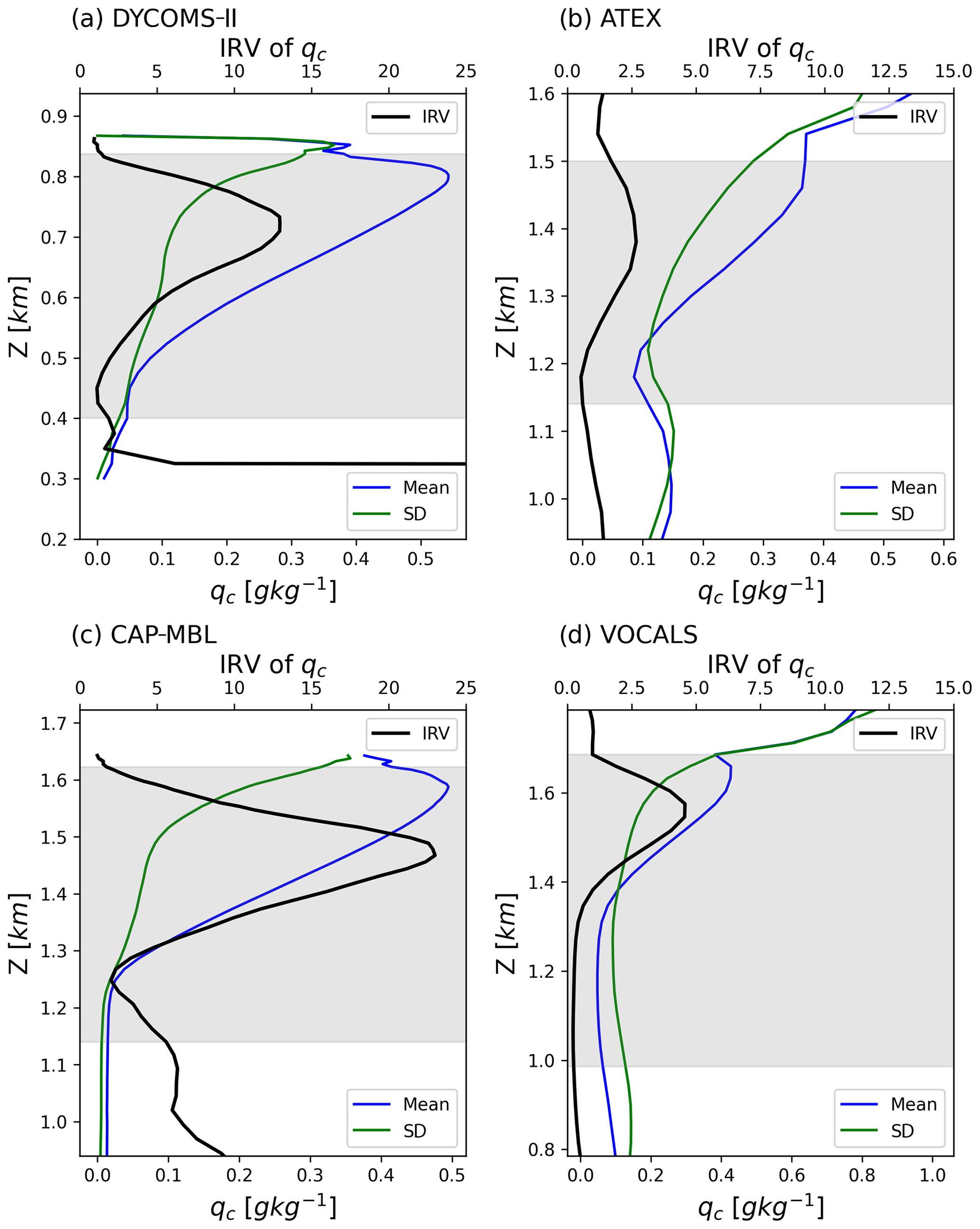
Although this study focuses on a single LES case that corresponds to the 18 July 2017 research flight in the ACE-ENA campaign (Zhang et al., 2021), the main findings listed above, in particular the shape of the vertical structure of LWC and its variance in Fig. 7a, should generalize to other cases of unbroken marine stratocumulus clouds. We illustrate the generality of the figure shapes in Fig. 11, which shows the vertical profiles of the q_c mean, standard deviation, and ${\mathit{\nu }}_{q_{\mathrm{c}}}$ calculated from four other LES cases of stratocumulus in the literature. These cases all employ explicit (bin) microphysics. The DYCOMS-II profiles (Fig. 11a) are based on a case of strongly drizzling stratocumulus over the northeastern Pacific sampled during the second research flight of the Second Dynamics and Chemistry of Marine Stratocumulus project (DYCOMS-II RF02; Ackerman et al., 2009). The profiles in Fig. 11b are calculated from LES output based on a case of stratocumulus with underlying cumulus from the Atlantic Trade Wind Experiment (ATEX; Stevens et al., 2001). Figure  11c is a case of November drizzling stratocumulus derived during the 22-month mobile deployment of the Department of Energy Atmospheric Radiation Measurement Program Mobile Facility (CAP-MBL; Remillard et al., 2017). Lastly, the profiles in Fig. 11d are calculated from LES output of a case of deep, strongly precipitating, decoupled stratocumulus over the southeastern Pacific (VOCALS campaign; Mechem et al., 2012). The shapes of the profiles of q_c mean, standard deviation, and ${\mathit{\nu }}_{q_{\mathrm{c}}}$ from these four different cases are similar to our profiles in Fig. 7a. This similarity strongly suggests that the shape of these profiles are decidedly controlled by the underlying cloud thermodynamics, dynamics, and microphysics, specifically the combined effect of adiabatic growth and cloud-top entertainment that are ubiquitous in marine stratocumulus clouds.

The strong vertical variation in E_q suggests that a constant, global value of E_q is an oversimplification, at least for a typical case of marine stratocumulus like we are exploring here. While some recently updated ESMs have the vertical resolution to resolve stratocumulus features and include a vertical dependence of E_q, many are too coarse and simply cannot. As such, in cases where an ESM must have a constant value of E_q, an E_q of 3.2 applied everywhere in the cloud is likely too large and should be reduced. In the middle and upper part of the cloud where autoconversion is most likely occurring, E_q has a smaller value between 1 and 1.5. Only near cloud base does E_q attain large values over 3.0, yet these regions have relatively little liquid water and, therefore, likely exhibit very little autoconversion.

This analysis considers only variability in cloud water q_c. A two-moment or size-resolving (bin) microphysical parameterization would take variability in N_c into account, which is a dependence that is also nonlinear (e.g., $N_{\mathrm{c}}^{-\mathrm{1.79}}$ in Khairoutdinov and Kogan, 2000). This additional nonlinear term provides an additional pathway for subgrid-scale variability bias, although recent work has demonstrated that the covariance between q_c and N_c largely counteracts the individual effects of q_c and N_c variability (Zhang et al., 2019, 2021). Extending this work using bin microphysics is the object of a future study, which will allow us to consider not only the nonlinearity associated with N_c but also the effect on the enhancement factor of homogeneous vs. inhomogeneous mixing regimes (at least down to the limited spatial and temporal scales associated with the model grid and time step) in the entrainment zone.