Regional PM_2.5 pollution confined by atmospheric internal boundaries in the North China Plain: boundary layer structures and numerical simulation

This study reveals mesoscale planetary boundary layer (PBL) structures under various pollution categories during autumn and winter in the North China Plain (NCP). The role of the atmospheric internal boundaries (AIBs, referring to the discontinuity of meteorological conditions in the lateral direction) in regulating PBL structures and shaping the PM_2.5 pollution patterns is emphasized. The Weather Research and Forecast (WRF) model is used to display the three-dimensional meteorological fields, and its performance is evaluated by surface observations and intensive soundings. The evaluation demonstrates that the model reasonably captures the mesoscale processes and the corresponding PBL structures. Based on the reliable simulations, three typical pollution cases are analyzed. Case 1 and case 2 represent the two main modes of the wind shear category pollution, which is featured with airflow convergence line/zone as AIB, and thus is dominated by dynamical effect. Case 1 presents the west–southwest wind shear mode associated with a trough convergence belt. The convergent airflow layer is comparable to the vertical scale of the PBL, allowing PM_2.5 transport to form a high pollution area. Case 2 exhibits another mode with south–north wind shear. A “lying Y-shaped” convergence zone is formed with a thickness of about 3000 m, extending beyond the PBL. It defines a clear edge between the southern polluted air mass and the clean air in the north. Case 3 represents the topographic obstruction category, which is characterized by a cold-air damming AIB in front of the mountains. The PBL at the foothills is thermally stable and dynamically stagnant due to the capping inversion and the convergent winds. It is in sharp contrast to the well-mixed/ventilated PBL in the southern plains, especially in the afternoon. At night, this meteorological discontinuity becomes less pronounced. The diurnal variation of the PBL thermal and dynamical structure causes the pollutants to concentrate at the foot of the mountains during the daytime and locally accumulate throughout the entire plain in the evening. These results provide a more complete mesoscale view of the PBL structure and highlight its spatial heterogeneity, which promotes the understanding of air pollution at the regional scale.

1 Introduction

The planetary boundary layer (PBL) is the lowest section of the atmosphere that responds directly to the heat and friction from the Earth's surface (Stull, 1988; Garratt, 1992). Most air pollutants are intensively emitted or chemically produced within this layer, and their horizontal transport and vertical mixing are affected by the dynamical flow and thermal stability of the PBL (Tennekes, 1974). Therefore, the PBL structure plays a crucial role in the evolution, magnitude and distribution of air pollution.

The PBL structure has been recognized to be strongly dependent on three categories of factors: (i) the single-column vertical property (such as turbulence intensity) forced by the local surface's energy balance; (ii) the lateral-section horizontal variation of wind, temperature and humidity regulated by the mesoscale meteorological process and (iii) the three-dimensional spatial evolution controlled by the large-scale synoptic system (Boutle et al., 2010). The local vertical PBL structure and its impact on air pollution have been widely discussed from different aspects including turbulent mixing (Emeis and Schafer, 2006; Ren et al., 2019), dynamical effect (Dupont et al., 2016), entrainment (Li et al., 2018; Jin et al., 2020), and radiative feedback with aerosol (Petäjä et al., 2016). In these studies, the PBL height at a certain site has been the most commonly used indicator to analyze the correlation with pollutant concentration, whether from the time scale of the diurnal cycle, daily variation, or longer period (Bianco et al., 2011; Liu et al., 2019; Miao and Liu, 2019). Moreover, some studies investigate the PBL spatial structure under the large-scale force of weather systems (Prezerakos, 1998; Boutle et al., 2010; Mayfield and Fochesatto, 2013). Sinclair et al. (2010) report that the three-dimensional PBL structure developed beneath an idealized mid-latitude weather system, which is characterized by a deep convective PBL in the eastern flanks of the anticyclone and a shallow shear-driven PBL in the cyclone's warm sector. The effect of the monsoon trough on the PBL has also been indicated, showing relatively low PBL capped by a stable layer in the western end of the trough line, with a well-defined deep moist layer with active thermal instability in the eastern end (Rajkumar et al., 1994; Narasimha, 1997; Potty et al., 2001). In recent years, synoptic classification has been used to explore the role of different weather circulations on PBL structure and to further analyze air pollution (Peng et al., 2016; Xiao et al., 2020). The movement of the synoptic systems makes the shallow and deep boundary layers develop alternately in a certain area, regulating the periodic evolution of large-scale air pollution.

At the intermediate scale, mesoscale systems interact with PBL in more direct and complex ways, since they occur in the lower troposphere with vertical extension comparable with the PBL depth and horizontal scale close to the regional range. Discontinuity of meteorological properties inside and outside these systems is presented as atmospheric internal boundaries (AIBs) in the lateral direction, usually manifested as temperature contrast and/or wind shift. Previous studies have emphasized their influence on the initiation of convective storms (Sanders and Doswell, 1995; Hane et al., 2002; Bluestein, 2008). On the other side, as internal lateral boundaries within the low-level atmosphere, the AIBs can lead to the abrupt change in the PBL spatial structure, which is of particular importance to the evolution of regional pollution. The effects of mesoscale sea–land and mountain–valley circulations on the PBL have been clarified, i.e., the thermal internal boundary layer in the coastal area and the depressed PBL close to a mountain base (Garratt, 1990; Lu and Turco, 1995; Talbot et al., 2007; De Wekker, 2008; Miao et al., 2015). Some studies discuss the PBL structure under the rule of other types of mesoscale/sub-synoptic scale systems, such as the persistent cold-air pools in the Salt Lake valley (Lareau et al., 2013), foehn winds in the Eastern Alps (Seibert, 1990; Baumann et al., 2001), and leeward troughs and cold-air damming around the Appalachian mountains (Seaman and Michelson, 2000; Bell and Bosart, 1988), as well as the frequent cold and warm fronts in Europe (Berger and Friehe, 1995; Sinclair, 2013). However, more understanding of their impact on the evolution of air pollution is needed.

The North China Plain (NCP) is one of the most polluted areas in the world. The dense population and developed industries produce intensive emissions in this region, with most sources located in the plain area and less in the northern and western mountains (their spatial distribution is presented in Fig. S1 in the Supplement). High-intensity primary emissions are the fundamental cause of air pollution, which directly releases pollutants into the atmosphere and provides precursors for secondary aerosol formation (Lyu et al., 2016; Zhao et al., 2019). In order to improve the air quality, a series of stringent emission reduction policies have been implemented from 2013, making the annual mean PM_2.5 concentrations decrease by 32 % in 2017 (Zhang et al., 2019). However, the severe polluted days still occur frequently, especially in winter (Zhang et al., 2018). During these pollution episodes, adverse meteorological conditions are the dominant factors causing high pollution levels and various spatial patterns, as there are no significant changes in emissions in a short period (e.g., weeks). Extensive studies have been conducted to investigate the meteorological causes of regional pollution in the NCP, such as the local meteorological factors and large-scale synoptic process (Ye et al., 2016; Ren et al., 2019; Li et al., 2020). Nevertheless, the knowledge about the PBL spatial structures under the impact of the mesoscale AIBs is still insufficient, and the role that the special PBL structures plays in the air pollution evolution at a regional scale is even unclear (Bluestein, 2008; McNider and Pour-Biazar, 2020).

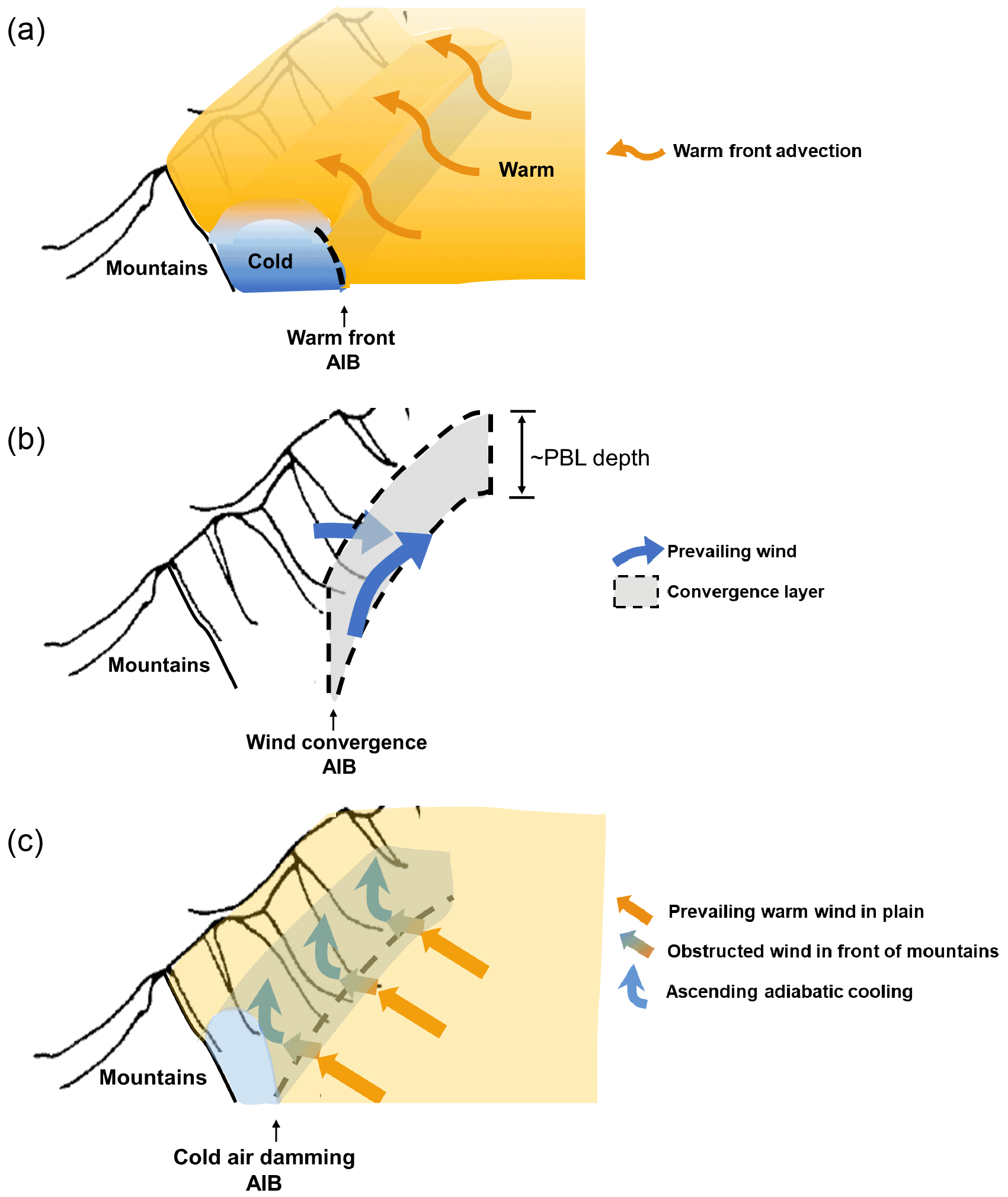
Figure 1 Schematic diagram showing the conceptual model of PBL spatial structures under three pollution categories. (a) Frontal category: the blue-shaded and orange-filled areas represent the isolated and stable cold air mass ahead of the warm front and the warmer well-mixing atmosphere behind the front. The orange arrows indicate warm front advection. (b) Wind shear category: two blue arrows represent the airflows ahead of and behind the trough. The gray-filled area indicates the dynamical convergence layer with a depth comparable to the boundary layer height. (c) Topographic obstruction category: the light-blue-filled area indicates the cold-air damming at the foot of the windward mountains. Terrain obstruction disrupts the geostrophic balance so that the southerly warm advection weakens (long orange arrows) and turns to the easterly cold advection (short gradient-color arrows), and meanwhile, the air mass accumulates to produce a lift cooling (upward blue arrows). Dashed black lines in (a–c) indicate the warm front AIB, wind convergence AIB, and cold-air damming AIB, respectively. The PBL spatial structure under the first category has been revealed by Jin et al. (2021). For the latter two categories, their PBL three-dimensional structures are discussed in Sect. 3.3 of this paper.

Based on the surface observations, a thorough survey of the PM_2.5 pollution categories under the control of the AIBs is carried out by Jin et al. (2022). It is found that the pollution formation–maintenance processes in the NCP can be classified into three categories, i.e., the frontal category, wind shear category and topographic obstruction category during the autumn and winter of the investigated 7 years (2014–2020). Figure 1 shows the schematic diagram of three pollution categories corresponding to various AIBs. The frontal category represents about 41 % of all 98 pollution episodes, and its PBL spatial structure has been revealed in a previous case study (Jin et al., 2021). It is characterized by an isolated cold air mass, which is laterally confined by mountains and warm front AIBs, and vertically covered by a warm dome (Fig. 1a). The strong elevated inversion depresses the PBL height abruptly to 200–300 m within the cold area in contrast to 600–800 m outside the zone, constituting adverse dispersion conditions and resulting in the most serious PM_2.5 pollution. The wind shear category is associated with airflow convergence AIB (Fig. 1b), which is dominated by dynamical effect and causes lighter PM_2.5pollution. West–southwest wind shear and south–north wind shear are the two main modes. The third category occurs when the airflow cannot cross the topographic obstruction and forms the cold-air damming AIB. A cold and heavy pollution belt develops at the foot of the windward mountains (Fig. 1c), under the synergistic effect of dynamical obstruction and thermal stratification. Although previous studies have classified the air pollution and revealed the spatial characteristics of the first category, the three-dimensional PBL structures interacting with AIBs under the other two categories are not yet clarified, which is responsible for 43 % of pollution episodes in the NCP. In order to bridge this knowledge gap, the present study deeply analyzes representative cases of the wind shear category and topographic obstruction category (detailed analyses in Sect. 3.3), and aims to provide a complete conceptual model of the PBL spatial structure in the NCP under various pollution categories and corresponding AIBs (Fig. 1).

The mesoscale meteorological models, such as the Weather Research and Forecast (WRF) model with the high spatial and temporal resolution, are plausible tools to capture the mesoscale systems and display detailed spatial structures in the lower atmosphere, including the AIBs and the PBL (Jimenez et al., 2016; Pielke and Uliasz, 1998; Seaman, 2000; Hanna and Yang, 2001; McNider and Pour-Biazar, 2020). The present study tries to reveal the thermal and dynamical structures of the PBL and their evolution associated with different AIBs in the condition of pollution episodes, by using the WRF model. For this purpose, the model performance is first evaluated with detailed sounding data from intensive experiments, ensuring the model's ability to reproduce the meteorological fields and their three-dimensional structures in the concerned region. The paper is organized as follows: the following section describes the PBL sounding observations as well as the WRF model settings. Section 3 provides an overview of representative pollution cases and the evaluation of the model performance. Furthermore, the PBL spatial structures under various pollution categories are analyzed. Finally, the conclusions are presented and the uncertainty of mesoscale numerical simulation is discussed in Sect. 4.

Figure 2 Geographical map of the (a) observation area and (b) WRF model domain. Intensive GPS soundings at Dezhou and Cangzhou (star), routine radiosonde sounding at Beijing (triangle) and air quality stations (plus) are indicated in (a). The rectangle in (a) is the same as the model inner domain d02 in (b).

2 Data and methods

2.1 Observations and data analysis

Intensive Global Positioning System (GPS) sounding data – two periods of field experiments were carried out to evaluate the meteorological model and explore wintertime PBL structure in the NCP: at Cangzhou (38^∘13^′ N, 117^∘48^′ E, Fig. 2a) from 8 to 28 January 2016 and at Dezhou (37^∘16^′ N, 116^∘43^′ E, Fig. 2a) from 25 December 2017, to 24 January 2018. The GPS radiosonde (Beijing Changzhi Sci & Tech Co. Ltd., China) was used to obtain profiles of wind speed, wind direction, temperature, and relative humidity with a vertical resolution of approximately 1 s (3–5 m). Eight soundings were taken on each day, at 02:00, 05:00, 08:00, 11:00, 14:00, 17:00, 20:00 and 23:00 LT (i.e., Local Time = Universal Time Coordinated + 8). The reliability of the GPS sounding data has been systematically evaluated by Li et al. (2020) and Jin et al. (2020, 2021).

Routine radiosonde sounding data – routine sounding data from the meteorological station of Beijing (39^∘56^′ N, 116^∘17^′ E, Fig. 2a) were collected during 7–12 October 2014, in the absence of intensive PBL observations. The data were obtained from Wyoming University, USA (http://weather.uwyo.edu/upperair/sounding.html, last access: 10 October 2021), and the original observation data with higher vertical resolution were provided by the China Meteorological Administration. The routine soundings were taken 2 times a day, at 08:00 and 20:00 LT.

The PBL height and vertical profiles – during the two periods of intensive field experiments, 160 and 240 datasets were collected at these two sites, including vertical profiles of temperature, relative humidity, wind speed and wind direction. We conducted quality control on the original sounding data, eliminated outliers and then calculated the profiles of potential temperature. All the profiles were smoothed by a three-point moving average method and were interpolated to obtain a vertical resolution of 10 m. The PBL height was derived via the potential temperature profile method and the detailed calculation followed the mathematical method established by Liu and Liang (2010). Sounding data were used to evaluate the model performance and to analyze the three-dimensional thermal and dynamical spatial structure of the PBL.

In addition to the PBL sounding data, routine meteorological observation and air quality monitoring data were used to obtain the surface meteorological field and pollutant concentration field. The spatial distributions of sea-level pressure, 10 m wind vector, potential temperature and the corresponding PM_2.5 concentration were obtained by data interpolation or diagnostic model; details of the methods were referred to Jin et al. (2021).

2.2 WRF model simulations

The WRF model was used to investigate the vertical and horizontal structures of the PBL. Two nested domains (Fig. 2b) were employed with horizontal grid resolutions of 15 and 5 km. Each domain had 37 vertical layers extending from the surface to 100 hPa, with 25 layers within 2 km (with the respective heights of about 9, 25, 50, 85, 120, 160, 200, 240, 290, 350, 420, 500, 580, 660, 740, 820, 900, 980, 1080, 1200, 1350, 1550, 1700, 1850, and 2000 m) to resolve the PBL structure. The meteorological initial and boundary conditions were set using the United States National Center for Environmental Prediction Final Analysis (NCEP-FNL) dataset. The physics parameterization schemes applied in this study were the same as Jin et al. (2021).

2.3 Representative cases

As mentioned above, PM_2.5 pollution episodes in the NCP are identified in the frontal category, wind shear category and topographic obstruction category, according to their association with the mesoscale AIBs (Jin et al., 2022). The present study tries to reveal the PBL structures modified by the AIBs under various pollution categories. Among them, the first category has been investigated previously (Jin et al., 2021). We focus on the representative cases under the other two categories in this paper. For the wind shear category, there are two main shear modes: west–southwest wind shear and south–north wind shear. Therefore, a total of three typical cases are selected to respectively represent these two pollution categories, i.e., case 1 for west–southwest wind shear mode – during 17–21 January 2018; case 2 for south–north wind shear mode – during 7–11 January 2016; and case 3 for topographic obstruction category – during 7–12 October 2014. The temporal and spatial evolution of their PM_2.5 concentrations and the corresponding surface meteorological conditions would be analyzed based on routine observations, and their PBL spatial structures would be revealed by the WRF model simulations.

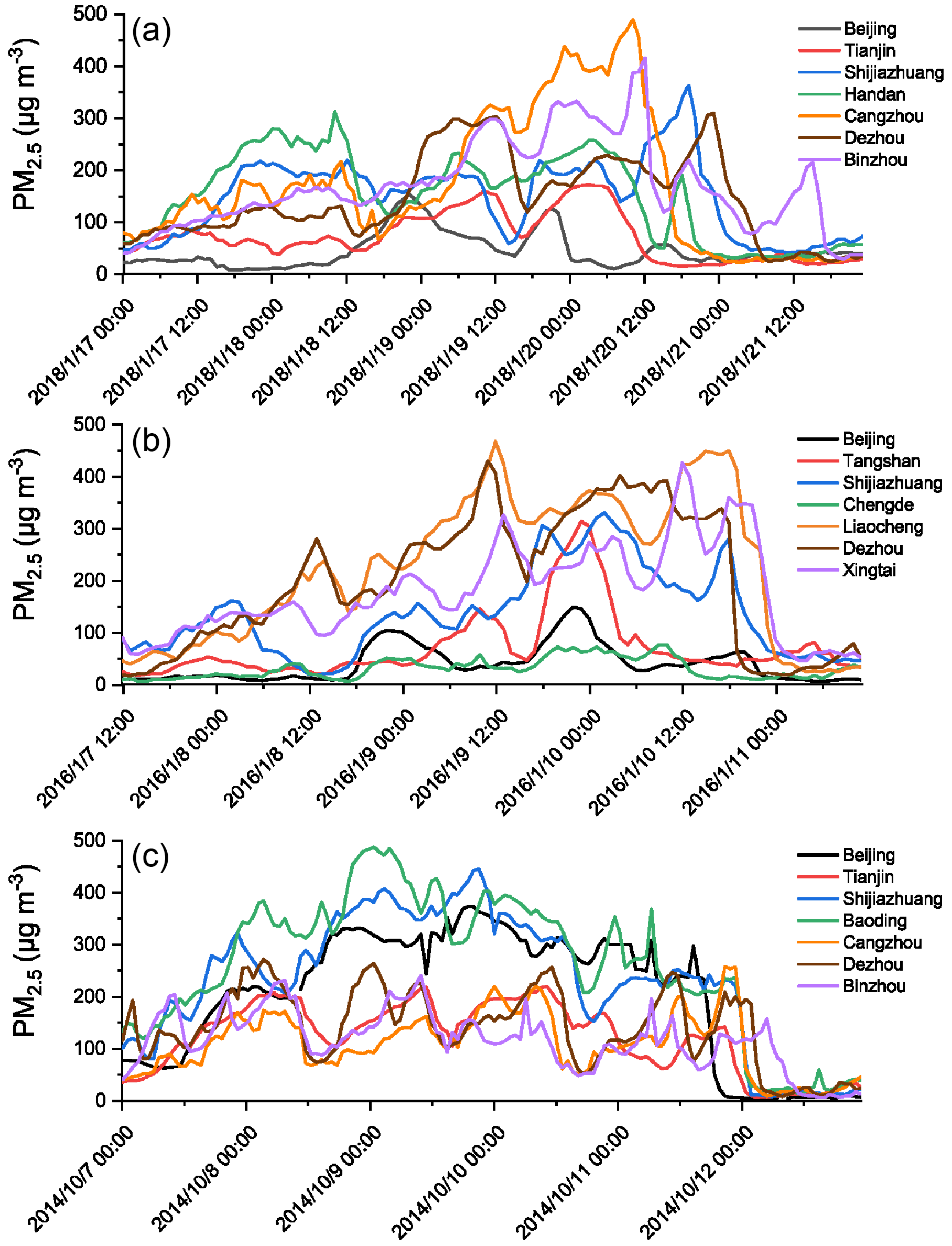
Figure 3 Temporal evolution of PM_2.5 concentrations during cases 1–3, respectively represent (a) west–southwest wind shear mode (17–21 January 2018), (b) south–north wind shear mode (7–11 January 2016), and (c) topographic obstruction category (7–12 October 2014). The locations of these PM_2.5 stations are marked in Fig. 2a.

3 Results

3.1 Basic features of the cases

Firstly, the surface observations for these three cases are presented. According to the temporal evolution of PM_2.5 concentrations at different stations in the NCP (Fig. 3), all three pollution episodes went through the stages of formation, maintenance and diffusion. As shown in Fig. 3a, case 1 was characterized by two main concentration peaks (300 µg m⁻³ at Handan vs 500 µg m⁻³ at Cangzhou) in the formation–maintenance stage (17–20 January 2018), with the latter being higher than the former. From noon on 20 January 2018, pollution in Tianjin–Cangzhou–Shijiazhuang diffused successively and all sites reached a clean level on the afternoon of 21 January 2018. For case 2, the pollution formed in the first 2 d, maintained over the next day and was cleaned on the night of 10 January 2016 (Fig. 3b). The southern sites such as Liaocheng and Dezhou were the most polluted (reaching 450 µg m⁻³), while the northern sites such as Beijing and Chengde were the least polluted (less than 150 µg m⁻³). Pollution in case 3 experienced the formation process on 7–8 October 2014, maintained for the successive 3 d, and ended on 12 October 2014 (Fig. 3c). During this period, the piedmont sites (Baoding, Beijing and Shijiazhuang) always held a high concentration regardless of day and night (about 400 µg m⁻³), while the southeast sites (Binzhou, Dezhou and Cangzhou) had lighter pollution and obvious diurnal cycle (lower than 250 µg m⁻³).

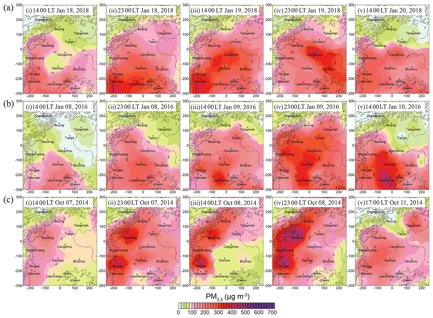
Figure 4 Spatial distributions of observed surface PM_2.5 concentrations (shaded colors) at the pollution stages of (i) formation, (ii–iv) maintenance, and (v) diffusion during representative cases 1–3 under (a) west–southwest wind shear mode, (b) south–north wind shear mode, and (c) topographic obstruction category. Values shown on x and y axes denote the distances (km) to the domain center. The PM_2.5 concentration fields are derived from spatial interpolation of pollution-observed data at monitoring stations.

The spatial patterns of PM_2.5 pollution, from the formation (Fig. 4i), maintenance (Fig. 4ii–iv), to the diffusion stage (Fig. 4v), are illustrated for each case. In the formation stage, the polluted air mass of case 1 and case 3 built up along the mountains from the southwest of the NCP, with the latter being more concentrated and the former being widespread in the south (Fig. 4a–i, c–i), while the pollution in case 2 first developed from the south (Fig. 4b–i). During the pollution maintenance process, case 1 was featured with extensive PM_2.5 flooding the NCP, resulting in the eastern region gradually being covered by heavy pollution (Fig. 4a, ii–iv); in case 2, a polluted air mass has been advancing northward with a clear edge, but it did not reach the northern mountainous area (Fig. 4b, ii–iv); the spatial distribution of PM_2.5 of case 3 was characterized by the day–night contrast, manifested as pollution filling the entire plain area at nighttime, while concentrating in front of the mountains with a distinct edge on the southeast side during the daytime (Fig. 4c, ii–iv). Finally, these pollution cases were diffused in different ways. In case 1, the clean air first occupied the northern parts of the NCP with a large concentration gradient on the front edges (Fig. 4a, v). As for case 2, PM_2.5 was restored to a clean level from the northeast (Fig. 4b, v). Pollution in the northwest was removed earliest in case 3, with Beijing acting as a loophole/passageway in the cleaning process (Fig. 4c, v). These cases presented various pollution distributions, however, all of them were characterized by clear edges or distinct heavy pollution cores.

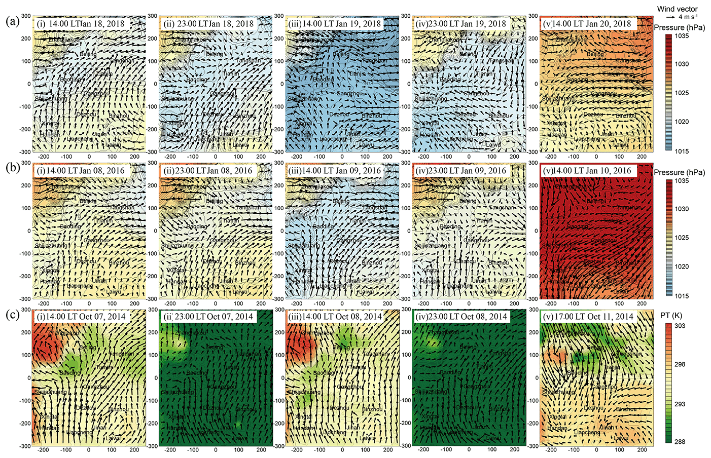
Figure 5 Observed sea-level pressure/potential temperature and wind vectors at the pollution stages of (i) formation, (ii–iv) maintenance, and (v) diffusion during representative cases 1–3 under (a) west–southwest wind shear mode, (b) south–north wind shear mode, and (c) topographic obstruction category. The shaded colors represent the sea-level pressure in (a–b) and the potential temperature in (c). The arrows indicate wind vectors. Values shown on x and y axes denote the distances (km) to the domain center.

The correspondent surface meteorological fields of the three cases are shown in Fig. 5. Case 1 and case 2 are the two main modes of wind shear category, for which dynamical AIB plays a dominant role, and thus the observed sea-level pressure and wind fields are discussed (Fig. 5a–b). Case 3 belongs to the topographic obstruction category. It is affected by the AIB created by the cold-air damming, and its potential temperature and wind fields are displayed to focus on the combined action of the thermal and dynamical properties (Fig. 5c). As shown in Fig. 5a, i–iii, the pollution formation and maintenance processes of case 1 were dominated by a leeward trough, which induced the westerly airflow shear to the southwest wind and produced a convergence belt at the trough axis. As the trough broadened and moved eastward, the wind convergence zone also moved (Fig. 5a, i–iii). On the evening of 19 January 2018, the leeward trough temporarily evolved into an inverted trough under the force of the approaching high pressure, creating a cyclonic convergence (Fig. 5a, iv). This explains why the heavy pollution expands eastward in this episode (refer to Fig. 4a, i–iv). Until 20 January 2018, a high-pressure system invaded the NCP from the northeast, bringing strong northeasterly winds (Fig. 5a, v), which in turn made the pollution disperse to the south (refer to Fig. 4a, v). During case 2, a saddle-shaped pressure field persisted in the pollution formation–maintenance stage and induced the prevailing northerly winds in the northern NCP against the dominant southerly flows in the southern area (Fig. 5b, i–iv). As a result, the polluted air mass was prevented from advancing northward to the mountains, causing a strong contrast in pollution concentration between the northern and southern parts of the domain (refer to Fig. 4b, i–iv). Its pollution diffusion process was also associated with a northeast high-pressure system, by strong northeasterly airflows cleaning up the PM_2.5 (Fig. 5b, v). As for case 3 under the topographic obstruction category, there was a narrow area with low potential temperature and weak southerly winds at the foot of the mountains on the windward side during the day, but this feature became fuzzy at night (Fig. 5c, i–iv). This diurnal variation repeatedly occurred during the formation and maintenance stages, corresponding excellently to the day–night difference in pollution distribution (refer to Fig. 4c, i–iv). In the end, the strong flows and cold air bursting like a jet stream through a pathway across Zhangjiakou–Beijing–Tianjin (Fig. 5c, v) led to pollutants being swept out from the northwest (refer to Fig. 4c, v).

3.2 Evaluation of simulated meteorological field

To reveal the PBL three-dimensional structure of these representative cases, numerical simulations are conducted using the WRF model. It is necessary to evaluate the model reliability before analyzing the simulated results. The model-observation comparisons in the previous studies usually focus on the time series of surface meteorological elements, such as 10 m wind speed and direction, 2 m temperature and humidity (Rogers et al., 2013; Bei et al., 2018; Qu et al., 2021). The model performance of their spatial fields is often ignored, and the simulated PBL vertical structure is rarely evaluated. However, the regional distribution and vertical structure of wind, temperature, and humidity are crucial for air pollution. And of course, the PBL height is a key parameter in characterizing air pollution ventilation conditions. In this study, the evaluation is carried out from three perspectives: (i) the temporal evolution, (ii) the spatial pattern of near-surface potential temperature and wind speed, and (iii) the vertical-temporal structure of these two variables at the sounding sites, in addition to the temporal variation of PBL height.

Table 1 Statistics of model performance for the hourly evolution of near-surface potential temperature and 10 m wind speed for the selected 13 cities during the representative cases.

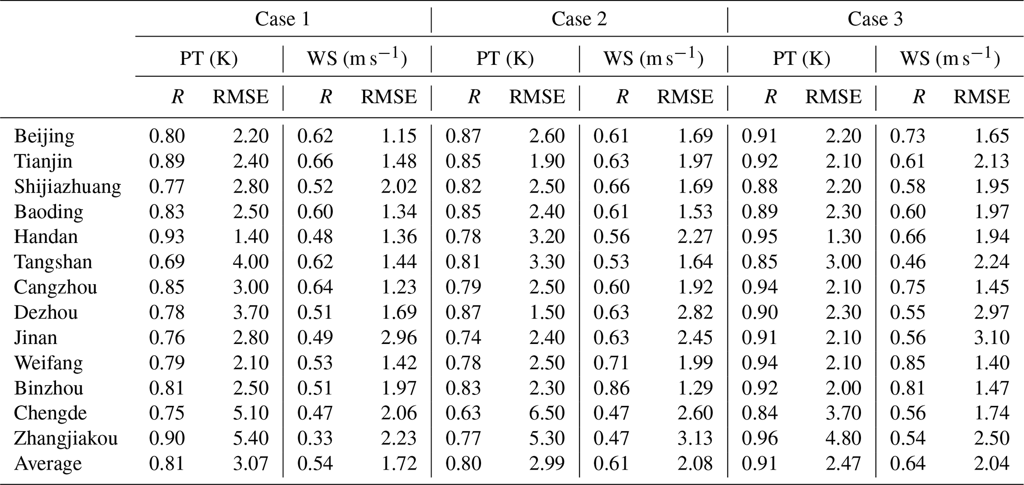
Case 1: west–southwest wind shear mode (17–21 January 2018); case 2: south–north wind shear mode (7–11 January 2016); case 3: topographic obstruction category (7–12 October 2014).

For the temporal evolution of the near-surface potential temperature and wind speed, the hourly observations and simulations of 13 key cities (Beijing, Tianjin, Shijiazhuang, Baoding, Handan, Tangshan, Cangzhou, Dezhou, Jinan, Weifang, Binzhou, Chengde and Zhangjiakou), evenly distributed in the NCP, are compared during these three pollution cases. The model outputs are extracted from the grid points nearest to the observed sites. As shown in Table 1, the correlation coefficients of the simulated and observed hourly evolution of potential temperature and wind speed are 0.80–0.91 and 0.54–0.64 (<0.01), respectively. In order to exclude the influence of the diurnal cycle on the correlation, the daily averages are also calculated and the obtained correlation coefficients are as high as 0.65–1 and 0.62–1 (<0.01) for potential temperature and wind speed, respectively (Table S1 in the Supplement). The statistical results demonstrate that the major variations in the time series of the surface observations are reproduced well by the model, which has also been recognized in previous studies (Rogers et al., 2013; Bei et al., 2018; Qu et al., 2021).

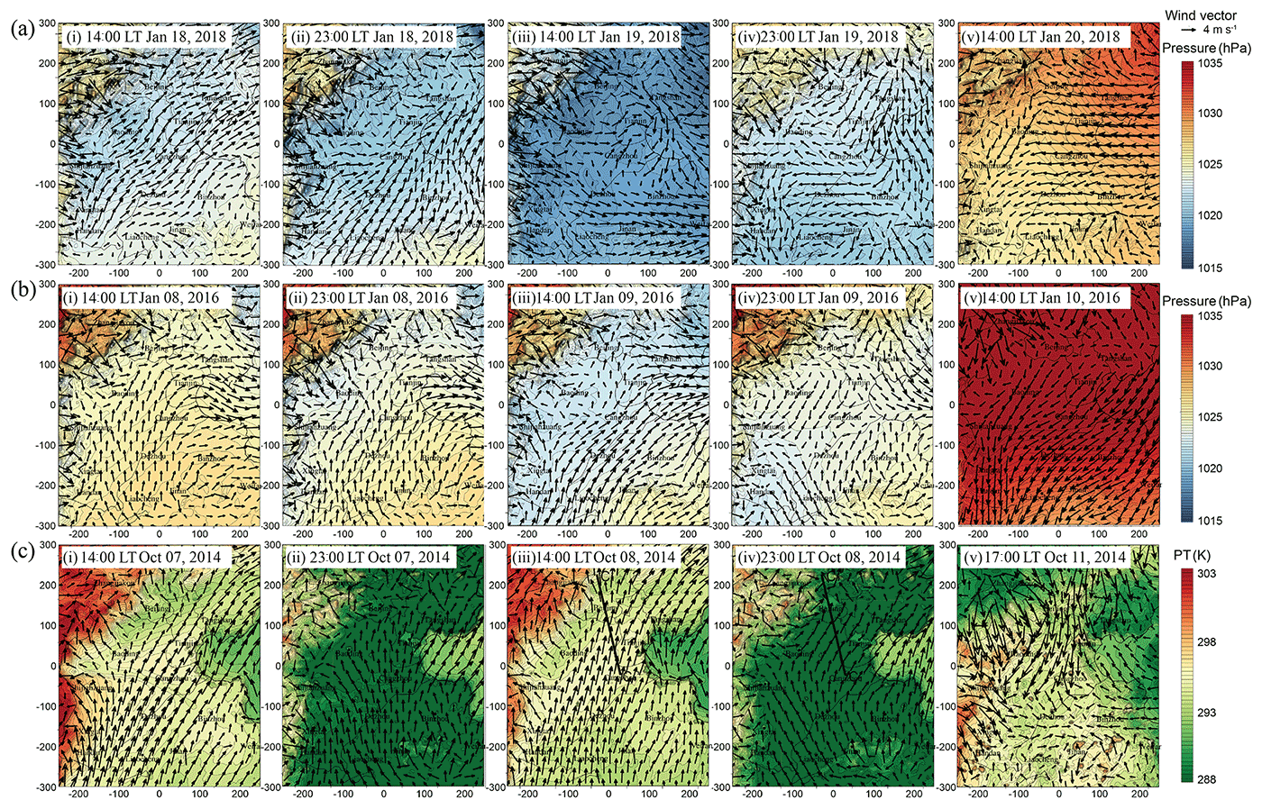
Figure 6 Simulated sea-level pressure/potential temperature and wind vectors at the pollution stages of (i) formation, (ii–iv) maintenance, and (v) diffusion during representative cases 1–3 under (a) west–southwest wind shear mode, (b) south–north wind shear mode, and (c) topographic obstruction category. The shaded colors represent the sea-level pressure in (a–b) and the surface potential temperature in (c). The arrows indicate wind vectors. Values shown on x and y axes denote the distances (km) to the domain center. Lines C₁C${}_{\mathrm{1}}^{\prime }$ in (c) refer to the cross sections of the potential temperature in Fig. 12.

Compared with Fig. 5, the simulated surface meteorological fields during the three cases are displayed in Fig. 6. In case 1 and case 2, the leeward trough and saddle-shaped pressure field, as well as the corresponding west–southwest wind shear and south–north wind shear are reproduced in the simulated fields (Fig. 6a–b, i–iv vs Fig. 5a–b, i–iv). Additionally, their movement and evolution during the pollution formation–maintenance processes are captured by the WRF model, although there are small deviations in the specific positions. At the diffusion stage, the simulated northeastern high-pressure and the prevailing easterly/northeasterly winds are comparable with the observed fields (Fig. 6a–b, v vs Fig. 5a–b, v). As for case 3, the modeling result of surface meteorological fields successfully reflect the narrow cold zone and stagnant wind belt at the foot of the mountains, as well as their diurnal variation and sustainability in the pollution formation–maintenance stage (Fig. 6c, i–iv vs Fig. 5c, i–iv). In the simulation field, the cold zone is shorter at its south end on the afternoon of 8 October 2014. There is also an overestimation of the potential temperature in the northwestern mountains and the Bohai Sea at night. At the end of this episode, a strong northerly cold airflow similar to the observation appears in the simulation field (Fig. 6c, v vs Fig. 5c, v). Generally, the main features of the surface distributions of meteorological observations during these three cases are reflected well in the simulated fields.

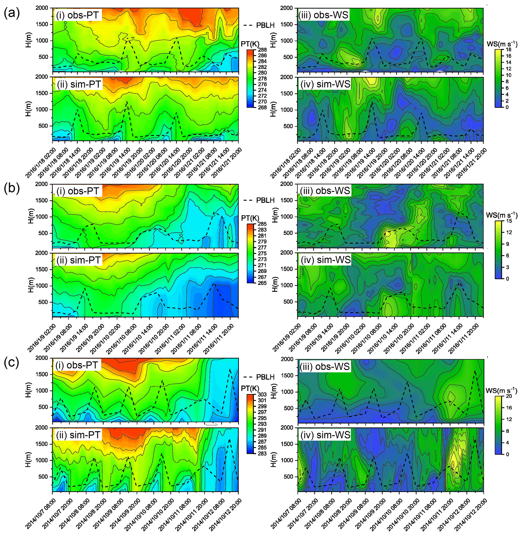
Figure 7 Observed and simulated time–height cross sections of potential temperature (left) and wind speed (right) during representative cases 1–3 under (a) west–southwest wind shear mode (18–21 January 2018), (b) south–north wind shear mode (9–11 January 2016), and (c) topographic obstruction category (7–12 October 2014). The dashed lines indicate the PBL heights. The observation data in (a–b) and in (c) are obtained from intensive sounding experiments and routine soundings, respectively.

Moreover, the simulated and observed time–height cross sections of potential temperature and wind speed, as well as the PBL height, are compared to reveal the model's ability to capture the atmospheric vertical structure of each case (Fig. 7). The observation data of case 1 and case 2 are obtained from intensive sounding experiments at the Dezhou and Cangzhou sites, respectively, while the observation information during case 3 is provided by routine soundings at the Beijing site. As for case 1, the model successfully reproduces the thermal structure evolution in the pollution formation–maintenance period, while the final uplift of the inversion layer and the growth of PBL are not well captured with an underestimation of about 200–300 m (Fig. 7a, i–ii). In comparison, the dynamical structures, the dominant roles in this category, are simulated much better. The vertical location and temporal transition of the strong and weak wind layers are comparable with observations (Fig. 7a, iii–iv). The correlation coefficient (R) between simulated and observed PBL height is about 0.68 (p<0.01). The model performance during case 2 is satisfactory both for cross sections of the potential temperature and wind speed. The formation and decay of upper temperature inversion and the development of the cold convective PBL are consistent between observation and simulation, though there are some underestimations in the modeled results (Fig. 7b, i–ii). The weak wind layer presented in the maintenance stage and vertical wind shear that occurred in the diffusion stage are also captured by the model with smaller gradients (Fig. 7b, iii–iv). Meanwhile, observed and simulated PBL heights show a consistent evolution with a correlation coefficient as high as 0.78 (p<0.01). Both of their PBL heights are lower during the pollution formation–maintenance stage and increase by more than 1000 m in the diffusion stage. In case 3, the WRF model reproduces the observed diurnal cycle of the potential temperature in the low level and the continuous warming at the upper layer during the formation–maintenance processes, as well as the replacement of a well-mixed cold air mass in the last phase (Fig. 7c, i–ii). The evolution of the simulated wind speed is roughly similar to the observation, including the maintenance of the calm wind layer in the first 4 d and the appearance of the final strong wind layer (Fig. 7c, iii–iv). Correspondingly, the PBL height is characterized by typical diurnal variations during the polluted period and begins to abruptly develop in the evening of 12 October 2014, associated with the cold air mass and strong wind, both in observation and simulation (R=0.81, p<0.01). Nevertheless, there are some inconsistencies in the details of observation and simulation evolution, which may result from the coarse resolution of routine soundings in time and vertical direction, in addition to the uncertainties of model simulation.

Overall, the model shows the ability to capture the observed mesoscale systems and atmospheric thermal and dynamical structures reasonably, both at the surface and in the vertical direction. With confidence in the model results, we now proceed to a detailed investigation of the PBL spatial structure affected by mesoscale AIBs under various pollution categories.

3.3 PBL spatial structure

We analyze the simulated vertical cross sections of the mesoscale systems and AIBs to reveal the three-dimensional structure of the PBL. Two key parameters, potential temperature and wind divergence, are used to respectively indicate the atmospheric thermal stability and dynamical convergence, in addition to another important parameter: the PBL depth. They directly affect the vertical mixing and horizontal transport of PM_2.5, and are critical for pollution formation and distribution.

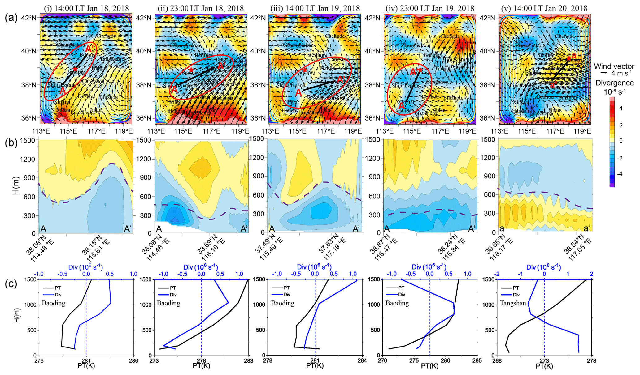
Figure 8 (a) Surface spatial distributions, (b) vertical cross sections and (c) vertical profiles of the simulated wind divergence at the pollution stages of (i) formation, (ii–iv) maintenance, and (v) diffusion during representative case 1 under west–southwest wind shear mode. The red ellipses, black lines, and red stars in (a) indicate the convergence belt, the section lines in (b), and the profile sites in (c), respectively. The dashed purple lines in (b) indicate the PBL heights. The potential temperature profiles are presented in (c) to indicate the boundary layer top at the representative sites.

3.3.1 Wind shear category

This pollution category, mainly involving two modes of west–southwest wind shear and south–north wind shear, is driven by dynamical flows. Therefore, for the corresponding case 1 and case 2, the wind divergence sections are analyzed in detail in the following (Figs. 8–9). The potential temperature sections are presented in the supplementary material (Figs. S2–S3), illustrating that there is no significant thermal discontinuity.

Figure 8 displays the PBL dynamical structure of case 1. During the pollution formation–maintenance stage, with the establishment of a low-pressure trough (refer to Fig. 6a), westerly winds shifted to southwesterly winds at the trough axis and thus formed a convergence belt at the surface with a divergence of −2 to $-\mathrm{4}\times {\mathrm{10}}^{-\mathrm{6}}$ s⁻¹ (Fig. 8a, i). As a consequence, a mass of pollutants were transported here and further accumulated to form a pollution zone (refer to Fig. 4a, i). This trough-convergence belt continued to move to the east, and evolved into a cyclonic-convergence center at the end of the maintenance phase (Fig. 8a, i–iv). During this process, its affected area was expanded so that the large range of the NCP was filled with pollutants (refer to Fig. 4a, ii–iv). The vertical section across the surface convergence belt shows that the depth of the convergence layer did not exceed 1000 m, with a compensating divergence layer immediately above it, being consistent with the evolution of the PBL (Fig. 8b, i–iv). Furthermore, the vertical profiles of the wind divergence and potential temperature at the Baoding site, located in the convergence belt, are extracted to illustrate the PBL dynamical structure more clearly. It shows that the mutation of divergence value and the jump of potential temperature roughly appeared at the same height (Fig. 8c, i–iv), which demonstrated that the vertical scale of the wind convergence belt was equivalent to the depth of the PBL. This phenomenon reveals that the west–southwest wind shear convergence caused by the trough mainly occurred within the PBL, reflecting its mesoscale property. In the process of pollution diffusion, with the advent of a northeast high-pressure system, divergent wind fields occurred correspondingly (Fig. 8a, v), which cleaned this part of the pollutants quickly (refer to Fig. 4a, v). The vertical cross section of this divergent layer and vertical profiles at the Tangshan site show that the northeast wind divergence layer was relatively thin with a thickness of no more than 600 m (Fig. 8b–c, v), implying that the removal of pollutants only occurred within the PBL.

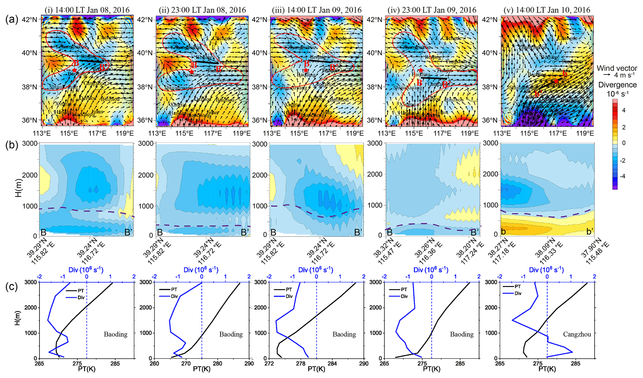
Figure 9 Same as Fig. 8, but for representative case 2 under south–north wind shear mode. The red lying-Y shapes, black lines, and red stars in (a) indicate the convergence belt, the section lines in (b), and the profile sites in (c), respectively. The dashed purple lines in (b) indicate the PBL heights. The potential temperature profiles are presented in (c) to indicate the boundary layer top at the representative sites.

As for the south–north wind shear mode, the surface divergence fields displayed a “lying Y-shaped” convergence zone with the opening to the west during the pollution formation–maintenance stage of case 2 (Fig. 9a, i–iv), which was caused by the meeting of the southerly and the northerly winds and then turning to the easterly winds. This convergence mode led to the distribution of pollutants in a concentration pattern that was much higher in the south and lower in the north, with a clear edge between these two air masses (refer to Fig. 4b, i–iv). Although the southerly winds in the southern NCP kept the pollutants transported northward, they never reached the northernmost part due to the opposite airflow there. The vertical cross sections of this special convergence zone exhibited a depth extending upwards for more than 3000 m, with a peak between 1000 and 2000 m above the PBL top (Fig. 9b, i–iv). Referring to the vertical profiles of wind divergence and potential temperature at the Baoding site, it can be seen that the depth of the convergence layer far exceeded the height of the PBL, whether it was during the day- or nighttime (Fig. 9c, i–iv). These phenomena demonstrate that the south–north wind shear created by the saddle-shaped pressure field is of much larger vertical and horizontal scales. The dynamical feature was no longer limited to the PBL, but extended to the sub-synoptic scales. In the pollution diffusion stage of this case, the PBL structure was the same as in case 1 (Fig. 9a–c, v), and has been described in the above paragraph.

To provide explicit support to the above explanation between the dynamical convergence feature and the pollution development, we adopt a chemical transport model (WRF-Chem) to simulate the PM_2.5 pollution process and directly quantify the advection term in the PM_2.5 concentration prognostic equation:

$$\begin{array}{}\text{(1)}& {\displaystyle \frac{\partial c}{\partial t}}=-\mathrm{\nabla }\cdot {\left(\mathit{U}c\right)}_{\text{adv}}+\mathrm{\nabla }\cdot {\left(K_{\text{e}}\mathrm{\nabla }c\right)}_{\text{diff}}+E_{\text{emiss}}+S_{\text{sink}}+R_{\text{chem}},\end{array}$$

where c is PM_2.5 concentration, U is the wind vector, and K_e is the turbulent diffusion coefficient. The first term on the right side of the equation represents the advection process both horizontally and vertically. The second term is turbulent diffusion, and the last three terms represent emissions, deposition and chemical reactions, respectively. The present study pays attention to the horizontal advection, which is considered to have an effect of utmost importance for the pollution development for the wind shear category. Details of the model configuration and validation are described in the Supplement (Sect. S1, Fig. S4, and Table S2).The simulations of case 1 and case 2 reproduce the PM_2.5 pollution concentration patterns and their evolution well. Their pollution formation and maintenance stages are discussed here. For case 1, the simulated near-surface PM_2.5 fields at 14:00 LT of both 18 and 19 January 2018, as well as their differences are displayed in Fig. 10a–c, indicating that the air pollution aggravates and spreads eastward. The temporal integration of the PM_2.5 horizontal advection term over this period (Fig. 10d) agrees well with the concentration increment pattern in Fig. 10c, demonstrating the crucial role of the dynamical convergence in the development of PM_2.5 pollution. The contribution of the horizontal advection term on the total increment of PM_2.5 concentration during this period over most of this region is very high, e.g., at Handan, Shijiazhuang, Baoding and Tianjin, the contribution ranges between 40 %–85 %. For case 2, heavy pollution is transferred to the north and east from 8 to 9 January 2016 (Fig. 10e–g). Similar to case 1, the advection term integrated over the pollution formation–maintenance period (Fig. 10h) presents good agreement with the PM_2.5 increment pattern (Fig. 10g). Quantitatively, this term contributes to total concentration accumulation as high as 27 %–80 % in the pollution process, especially in Beijing, Tianjin and Baoding. This result is also consistent with those in previous works (Jiang et al., 2015; Chang et al., 2019; Jin et al., 2020). The above analysis indicates that the airflow convergence AIB does not sharply confine the pollution air mass, but provides a circumstance or structure for pollutants transporting/accumulating along or nearby this zone. Due to of the dynamical property, the concentration fields of the wind shear category pollution are more variable in space and time.

Figure 10 Simulated (a–b, e–f) near-surface PM_2.5 concentrations at two instants during the pollution formation–maintenance stage and (c, g) their difference, as well as (d, h) the temporal integration of the PM_2.5 horizontal advection term over this stage for case 1 (upper) and case 2 (lower).

3.3.2 Topographic obstruction category

As an outcome of a mixture of the thermal and dynamical effects, the topographic obstruction category pollution is analyzed from the perspectives of both the wind divergence and potential temperature to reveal the dynamical and thermal structure of the PBL.

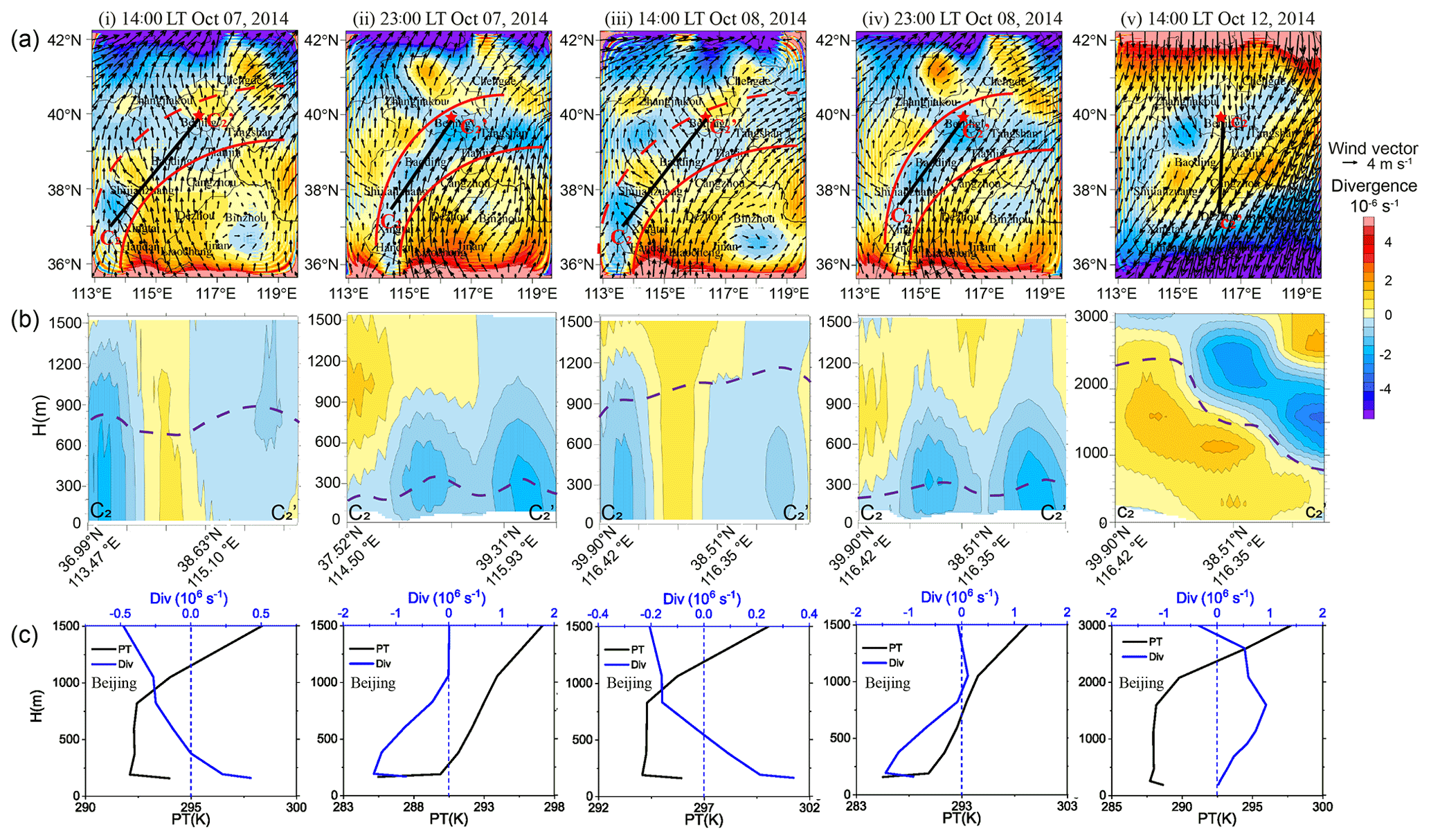
Figure 11 Same as Fig. 8, but for representative case 3 under the topographic obstruction category. The red curves, black lines, and red stars in (a) indicate the convergence belt, the section lines in (b), and the profile sites in (c), respectively. The dashed purple lines in (b) indicate the PBL heights. The potential temperature profiles are presented in (c) to indicate the boundary layer top at the representative sites.

Figure 11 shows the dynamical characteristics of the PBL during case 3. In the pollution formation–maintenance stage, there was an arc-shaped convergence belt at the foot of the mountains on the windward due to the momentum loss in the northward flow under the action of topographic obstruction (Fig. 11a, i–iv). The shape of this convergent belt was more regular at night (Fig. 11a, ii, iv) but had some breakages at the northern edge during the day when there was a local southeasterly wind around Beijing and Shijiazhuang (Fig. 11a, i, iii). The vertical sections also displayed the general features and diurnal difference, showing an integral convergence layer at night with a depth of the mountain height (Fig. 11b, ii, iv), and an isolated divergent layer emerged during the daytime (Fig. 11b, i, iii). The vertical profiles of the wind divergence and potential temperature at Beijing were further shown in Fig. 11c, i–iv. In the evening, the atmosphere below 1200 m was convergent with the peak appearing near the surface of about $-\mathrm{1.5}\times {\mathrm{10}}^{-\mathrm{6}}$ s⁻¹. In the afternoon, there was a weak divergence layer with a strength of about $\mathrm{0.5}\times {\mathrm{10}}^{-\mathrm{6}}$ s⁻¹ and a thickness of about 200–300 m within the PBL. We infer that the day–night variation may be the consequence of the mountain–valley circulation, since the northwestward daytime valley wind developed along the mountain gorges near Beijing and Shijiazhuang leading to flow divergence, and downslope winds formed at night, strengthening the surface convergence. During the pollution diffusion stage, the northern part of the domain was in a strong divergence condition (Fig. 11a, v). The corresponding cross section shows that the north wind divergence layer was very deep (nearly 3000 m), even extending beyond the boundary layer. It gradually thins from north to south with the decrease of the PBL height (Fig. 11b, v). Moreover, the vertical profiles of the divergence and potential temperature at the Beijing site show that the PBL was well developed up to 2000 m, accompanied by strong horizontal divergence throughout the layer (Fig. 11c, v); both of them indicate extremely favorable ventilation conditions.

The thermal properties and their evolution, especially diurnal variation, play an important role in this pollution pattern, which has been presented in the above surface analysis. Hence, we further explore the three-dimensional thermal structure of the PBL, taking the vertical cross sections of potential temperature across the characteristic cold area in the pollution maintenance stage (8 October 2014, the location of the cross section is shown in Fig. 6c) as an illustration. In the early hours of the morning, although there were surface inversions across the whole region, the cold air masses in front of the mountains were much thicker (Fig. 12a, i). After sunrise, the convective boundary layer developed both in the front of the mountains and in the plain due to the surface heating, but the temperature in the southern plain was higher and the PBL was slightly deeper (Fig. 12a, ii). In the afternoon, a deep, well-mixed warm PBL (with a height of more than 1000 m) formed in the southern plain, while a cold air mass capped by strong inversion (at the height of about 600–1000 m) still remained in the northern area (Fig. 12a, iii). At night, large amounts of cold air accumulated at the foot of the mountains again (Fig. 12a, iv). The vertical profiles of the simulated potential temperature of the three sites from south to north (Jinan, Cangzhou and Beijing), also support this thermal evolution process. At 02:00 LT, there were surface inversions at all three cities, and Beijing had the strongest inversion intensity of about 2 K per 100 m (Fig. 12b, i). By 10:00 LT, the PBL height in Jinan had increased to 1100 m, while the convective boundary layers in Beijing and Cangzhou were shallow (about 400 m, Fig. 12b, ii). In the afternoon, the PBL was fully developed with the height from the south to the north ranging from 1150 to 650 m, and there was still a thick inversion layer above Beijing (Fig. 12b, iii). At 23:00 LT, the surface inversion at the three sites had formed again (Fig. 12b, iv). The persistent cold air mass in front of the mountains is similar to the cold-air damming on the eastern side of the Appalachian mountains (Bell and Bosart, 1988). The prevailing southerly warm airflows were blocked by the mountains and the geostrophic balance was disrupted, so that the heat cannot reach the foothills and the air was further cooled due to the turning easterly wind. Meanwhile, the air mass accumulated and ascended with adiabatic cooling in front of the mountains. It should be noted that the southeast edge of this cold area was more pronounced during the daytime (Figs. 5c, 12), in comparison to that at night. This is reasonable, given that the nocturnal boundary layer was stable over the entire domain and more susceptible to the local property, such as surface heterogeneity, meandering motions and gravity waves (Mahrt, 1998). Although the AIB was relatively unclear at the surface during nighttime, the nocturnal cold layer at the foothills was deeper than the southern plain area, probably due to the cold drainage flows along the sidewall of the mountains to form a cold air pool. This diurnal cycle of the PBL thermal structure can well explain the day–night difference in pollution distribution pattern (refer to Fig. 4e).

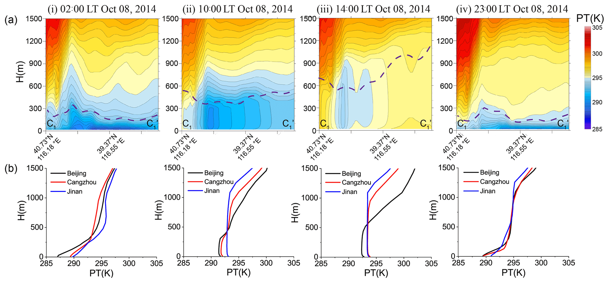
Figure 12 (a) Vertical cross sections and (b) vertical profiles of the simulated potential temperature at (i) 02:00 LT, (ii) 10:00 LT, (iii) 14:00 LT and (iv) 23:00 LT on 8 October 2014 in case 3 under the topographic obstruction category. The cross sections along the line C₁C${}_{\mathrm{1}}^{\prime }$ are shown in Fig. 6c, iii, iv. The dashed purple lines in (a) indicate the PBL heights.

4 Summary and discussion

This study investigated the three-dimensional PBL structures modified by mesoscale AIBs under various pollution categories by using the mesoscale meteorological WRF model. Based on the classification of pollution episodes in the NCP (Jin et al., 2022), representative pollution cases of the wind shear category and topographic obstruction category were analyzed. The WRF model was comprehensively evaluated for its reliability, by comparison with observed PBL vertical structure, as well as the temporal series and spatial distribution of the surface meteorological fields. The evolution of the PBL spatial structures and their interaction with the mesoscale AIBs during the pollution episodes were fully revealed, from both thermal and dynamical perspectives.

The results of this paper, together with a previous systematic classification study (Jin et al., 2022) and a detailed case study for frontal category (Jin et al., 2021), depict a clearer and more complete view of the PBL spatial structures during pollution episodes in the regional scale of NCP (as schematically shown in Fig. 1). All the pollution conditions during the autumn and winter seasons were classified into three categories. The most prominent was the frontal category. With an isolated cold air mass laterally bounded by the warm frontal AIB on one side and mountains on another side, the PBL was vertically suppressed by a dome-like warm cap. Typically, the intensity of the frontal inversion can be as large as 3–6 K per 100 m. As a consequence, the PBL in this cold area was very shallow (as low as 200–300 m) and kept the stratification stable, in sharp contrast to the deep and well-mixing boundary layer outside this zone (Fig. 1a). This explained why PM_2.5 accumulated rapidly in this enclosed and stable space and formed a laterally, clearly defined polluted air mass. Diurnally, the nocturnal PBL in this category was less typical than its daytime counterpart. The thermal structure of the PBL played a leading role in this category, resulting in the most severe pollution level.

The wind shear category, with two main modes, i.e., west–southwest wind shear and south–north wind shear, was featured with airflow convergence AIB and dominated by dynamical processes. The first mode was characterized by a low-pressure trough. A convergence layer lay in the wind shear zone with the thickness of the PBL depth (Fig. 1b), and a typical near-surface divergence of −2 to $-\mathrm{4}\times {\mathrm{10}}^{-\mathrm{6}}$ s⁻¹. It is accompanied by a compensating divergence layer above the PBL, reflecting the mesoscale property of the trough AIB. The latter mode displayed a lying Y-shaped convergence layer from the surface extending upwards to about 3000 m, with a convergence peak above the PBL top (not shown in Fig. 1). This implied the sub-synoptic scale features. In both modes of this category, the boundary layer was dominated by dynamical convergence effects, which resulted in the transport and accumulation of pollutants and thus drove the variation of the PM_2.5 distribution. This corresponds to relatively light pollution in the NCP.

The topographic obstruction pollution category was characterized by a cold air damming AIB at the foot of the windward side of the mountains. It usually occurred when the southerly winds were too weak to cross the terrain barrier and the northward flows were blocked. In response, the geostrophic balance was adjusted, which made the southerly warm advection weaken and further turned to easterly cold advection. All these factors allowed air masses to accumulate and ascend with adiabatic cooling at the foothills. The PBL air was cold and capped by a strong inversion in the damming area, in contrast with well-mixed warm PBL in the southern plain. Meanwhile, the air flows were convergent in front of the mountains. These general characteristics are shown in Fig. 1c. In more detail, the thermal discontinuity became indistinct at night due to the surface inversion over the entire domain, while the nocturnal wind convergence belt was more pronounced. The diurnal variation of the PBL dynamical and thermal structures made the pollutants concentrate at the foot of the mountains during the daytime while local pollution formed throughout the entire plain at night.

The present study focuses on the characteristics of mesoscale PBL structures under pollution conditions, and emphasizes their role in shaping regional pollution patterns. The analysis of pollution evolution is based on the PM_2.5 concentration fields interpolated or diagnosed from monitoring data, relying on densely distributed stations. However, the PBL spatial structure is presented by numerical simulation, due to the scarcity and limitation of sounding data. Evaluation from the spatiotemporal variation of the surface meteorological field and PBL vertical structure indicates that the model performance is good. The WRF model can capture mesoscale systems and AIBs, as well as their overall evolution process and diurnal variation. It should be noted that it is still difficult to reproduce the precise timing of the buildup and breakup as well as the exact location and range of these systems. This deficiency should be seriously concerned when simulated meteorological fields are used to drive air quality models, since a small position bias and time deviation of the AIBs can significantly alter pollution levels at a certain site (Seaman, 2000; McNider and Pour-Biazar, 2020). Accurate capture of mesoscale AIBs is a necessary prerequisite for reliable simulation of pollution evolution. Furthermore, successful reproduction and forecast of air quality by the chemical transport models also involve other factors, such as the accuracy of source inventories and the complexity of chemical mechanisms (Travis et al., 2016; Bouarar et al., 2019; Wang et al., 2021), which are beyond the scope of this study. Keeping all these in mind, we conducted supplementary chemical transport simulations and explicitly demonstrated the role of the airflow convergence AIB in the formation of wind shear category pollution.

Finally, the pollution categories presented in this study can still be rough or oversimplified, and the real processes may be more complex and atypical as analyzed. However, this paper, to the authors' knowledge, is the first trial to reveal the various PBL structures over the vast scale of the NCP, and to clarify their role in regional PM_2.5 pollution. Modulation of the PBL by mesoscale meteorological processes, particularly the AIBs, is clearly demonstrated. Extending the view of the PBL from local vertical properties to mesoscale three-dimensional structures may be a step toward a better understanding of the meteorological effects on regional-scale PM_2.5 pollution.