the Creative Commons Attribution 4.0 License.
the Creative Commons Attribution 4.0 License.
 | 31 Aug 2022
Dynamical perturbation of the stratosphere by a pyrocumulonimbus injection of carbonaceous aerosols
Giorgio Doglioni
Valentina Aquila
Sampa Das
Peter R. Colarco
Dino Zardi
The Pacific Northwest Pyrocumulonimbus Event (PNE) took place in British Columbia during the evening and nighttime hours between 12 and 13 August 2017. Several pyroconvective clouds erupted on this occasion, and released in the upper troposphere and lower stratosphere unprecedented amounts of carbonaceous aerosols (300 ktn). Only a few years later, an even larger pyrocumulonimbus (pyroCb) injection took place over Australia. This event, named “the Australian New Year (ANY) event”, injected up to 1100 ktn of aerosol between 29 December 2019 and 4 January 2020. Such large injections of carbonaceous aerosol modify the stratospheric radiative budgets, locally perturbing stratospheric temperatures and winds. In this study, we use the Goddard Earth Observing System Chemistry Climate Model (GEOS CCM) to study the perturbations on the stratospheric meteorology induced by an aerosol injection of the magnitude of the PNE. Our simulations include the radiative interactions of aerosols, so that their impact on temperatures and winds are explicitly simulated. We show how the presence of the carbonaceous aerosols from the pyroCb causes the formation and maintenance of a synoptic-scale stratospheric anticyclone. We follow this disturbance considering the potential vorticity anomaly and the brown carbon aerosol loading and we describe its dynamical and thermodynamical structure and its evolution in time. The analysis presented here shows that the simulated anticyclone undergoes daily expansion–compression cycles governed by the radiative heating, which are directly related to the vertical motion of the plume, and that the aerosol radiative heating is essential in maintaining the anticyclone itself.
- Article
(13207 KB) - Full-text XML
- BibTeX
- EndNote


Wildfires release large quantities of water vapor and aerosols in the atmosphere as well as carbon oxides and other gases (Wiedinmyer et al., 2011). Under favorable atmospheric conditions, the rising of plumes from the wildfire can reach the stratosphere, as shown by Peterson et al. (2018) and Fromm et al. (2000, 2010). This lofting to the stratosphere is driven by different mechanisms. First, as soon as the plume reaches its lifting condensation level, the release of latent heat from the condensation of water vapor results in its further buoyant rise. This process is referred to as pyroconvection and produces pyrocumulus (pyroCu) clouds. Then, if the state of the troposphere is conducive to the formation of dry thunderstorms (Peterson et al., 2017), pyroCu clouds can further develop vertically, reaching the tropopause and evolving into pyrocumulonimbus (pyroCb) clouds, i.e., wildfire-driven thunderstorms loaded with smoke from the wildfire (Fromm et al., 2010).
A distinctive feature of pyroCb clouds is the transport of wildfire by-products to the upper troposphere and lower stratosphere (UTLS): these thunderstorms act as chimneys, promoting the accumulation of aerosols and other gases in the UTLS. Once in the stratosphere, the main depletion mechanisms for aerosols (i.e., wet and dry deposition) are greatly reduced compared to the troposphere, and, as a consequence, aerosols have a significantly longer lifetime than in the troposphere (Yu et al., 2019). In the UTLS, the optically thick carbonaceous aerosols from wildfires absorb radiation, causing the temperature of the smoke plume to rise. This warming results in a gradual diabatic lofting of the plume itself (Torres et al., 2020; Das et al., 2021). This process is more pronounced in the days following the aerosol injection into the UTLS, when the concentration of aerosol is higher (de Laat et al., 2012; Ditas et al., 2018).
The second largest pyroCb aerosol injection ever recorded is the 2017 Pacific Northwest Event (PNE). The PNE was characterized by an outbreak of seven pyroCb clouds in British Columbia, Canada, and the state of Washington, USA during the evening of 12 August 2017 and the first hours of the following day (Peterson et al., 2018; Fromm et al., 2021). Overall, the pyroCb outbreak injected into the stratosphere an unprecedented smoke plume, whose mass was estimated to be between 0.1 and 0.35 Tg (Peterson et al., 2018; Torres et al., 2020). This record was surpassed by the injection from the December 2019/January 2020 Australian New Year event (ANY), which resulted in the stratospheric injection of up to 1.1 Tg of aerosol (Peterson et al., 2021).
Several studies (Das et al., 2021; Bourassa et al., 2019; Kloss et al., 2019; Torres et al., 2020; Yu et al., 2019; Christian et al., 2019; Baars et al., 2019) have characterized the aerosol plume from the PNE event and its interaction with large-scale stratospheric features, such as the Asiatic Summer Monsoon Anticyclone. In the days following the PNE, the smoke gradually rose into the stratosphere due to diabatic heating, with peak ascent rates of 2–3 km d−1 (Das et al., 2021; Torres et al., 2020). The plume eventually reached 22 km in height around 20 d after the injection, as detected in OMPS LP (Ozone Mapping and Profiling Suite, Limb Profiler) and SAGE III (Stratospheric Aerosol and Gas Experiment) observations (Torres et al., 2020; Bourassa et al., 2019). The plume was also detected by ground-based lidars, as presented in Khaykin et al. (2018). The smoke remained in the atmosphere for several months, with an estimated half-life of 5 months (Christian et al., 2019; Yu et al., 2019); during this period it perturbed the radiative balance of the atmosphere, causing global mean radiative forcing anomalies at the surface of the order of W m−2 during September 2017 (Das et al., 2021). Lestrelin et al. (2021) analyzed the dynamical features of the PNE plume by inspecting ERA5 reanalysis fields and CALIOP (Cloud-Aerosol Lidar with Orthogonal Polarization) measurements, finding that it evolved into stratospheric anticyclones that persisted for almost 2 months.
These smoke-induced stratospheric anticyclones were first reported following the ANY event (Allen et al., 2020; Kablick et al., 2020; Khaykin et al., 2020; Lestrelin et al., 2021) and have been termed “SWIRLs” (Smoke With Induced Rotation and Lofting) by Allen et al. (2020). These studies underline the stability of the SWIRLs and their resilience against the large-scale shear characterizing the background wind field. The main signatures of SWIRLs are a deep potential vorticity anomaly with respect to the zonal mean (negative in the Northern Hemisphere, positive in the Southern Hemisphere) and an associated anticyclonic motion, enhanced optical thicknesses, and a vertical temperature anomaly dipole. Also, the SWIRL encases air from the UTLS with low ozone content and this is reflected in a characteristic negative ozone concentration anomaly as the SWIRL moves upward. As pointed out by Khaykin et al. (2020), the SWIRL effectively traps the carbonaceous aerosol, with the result of efficiently transporting it to higher altitudes. The cited studies underline how the presence of carbonaceous aerosol is the necessary condition in the formation and maintenance of SWIRLs and how the coupling between aerosol, radiation, and dynamics is necessary to reproduce a SWIRL in model simulations (Khaykin et al., 2020; Allen et al., 2020).
In this work we use a chemistry climate model to simulate the impact on the stratosphere of a pyroCb plume from an event of the magnitude of the 2017 PNE, as well as the effect of the aerosol radiative interaction in the development of the plume itself. As in Das et al. (2021), we use the Goddard Earth Observing System Chemistry Climate Model (GEOS CCM), focusing in this study on the GEOS Atmospheric General Circulation Model configuration with prognostic aerosols from the GOCART (Goddard Chemistry, Aerosol, Radiation, and Transport) module to simulate the long-term transport of the plume and its impact on the radiative budget of the atmosphere. While Das et al. (2021) used GEOS CCM in a relaxed replay mode, i.e., driven by observations in the troposphere, we present here free-running simulations (i.e., weather forecasts). In previous work by Khaykin et al. (2020), Allen et al. (2020), and Lestrelin et al. (2021), the structure of the SWIRL was reproduced and maintained thanks to the assimilation of the observations and not by the local radiative heating caused by the carbonaceous aerosols. Here, we show how the GEOS CCM is capable of forming and maintaining a SWIRL following a stratospheric aerosol injection, such as the one from the PNE event, thanks to its representation of the radiative impact of the aerosol on the dynamics.
The choice of the free-running configuration is driven by the need to unambiguously resolve the dynamical and thermodynamical impact of the radiative heating by the aerosol. Indeed, the absence in the simulations of replay (or nudging) to a reanalysis ensures that any perturbation connected to the presence of the aerosol comes from the aerosol itself and not from underlying reanalysis fields or measurements. However, simulations in the free-running configuration will not necessarily reproduce the real-world smoke transport, because the simulated meteorological fields will differ from the observed fields. This impedes a thorough comparison between observed SWIRLs and the simulated one, but we show in Sect. 3 how a free-running simulation still reproduce SWIRLs with realistic characteristics.
The article is structured as follows. In Sect. 2 we briefly describe the GEOS model as well as the setup used for the simulation. In Sect. 3 we present the results from the simulations, analyzing the dynamical signatures and thermodynamical characteristics of the reproduced SWIRL and comparing them with previous works; more specifically, we analyze the anomalies of potential vorticity, wind, temperature, and geopotential that describe the SWIRL as well as their evolution during the SWIRL life; moreover, we show how the diabatic heating provided by the presence of the aerosol is correlated with the dynamics of the SWIRL itself, and how the SWIRL undergoes a daily expansion–compression cycle following this diabatic heating. Also, the geometrical characteristics of the SWIRL are pointed out, and we compare the resulting dimensions with the SWIRLs observed in previous works. In Sects. 4 and 5 we present some considerations about the reproduced SWIRLs and draw conclusions about the novelty and limitations of this work in comparison with other studies.
2.1 Model description and simulation setup
The Goddard Earth Observing System (GEOS) can simulate atmospheric circulation and chemistry, oceanic circulation and biogeochemistry, land surface processes, and data assimilation at horizontal resolutions as small as 12 km (Molod et al., 2015; Rienecker et al., 2008). In this study we use GEOS as an atmospheric general circulation model, resolving the atmospheric circulation and composition, but using prescribed sea surface temperatures and sea ice fractions. GEOS can be used either in replay or in free running configurations. In the replay mode, simulations are constrained by the MERRA-2 reanalysis fields, while in the free-running mode the evolution of the atmosphere is not constrained to the observations. The results shown in this study were produced in free-running simulations with the Icarus 3.3 version of GEOS. The meteorological fields for the model initialization on the 13 August (00:00 Z) were obtained from version 2 of the Modern-Era Retrospective Analysis for Research and Applications (Gelaro et al., 2017).
Simulations were run on a cubed-sphere horizontal grid with horizontal resolution of ∼50 km with 72 hybrid vertical sigma levels extending from the surface to 0.01 hPa (Rienecker et al., 2008). Aerosol concentrations and aerosol processes are simulated with the GOCART module, a bulk aerosol module simulating the evolution of black carbon (BC), brown carbon (BrC), organic carbon (OC), nitrates (NO3), sulfates (SO4), dust, and sea salt (Chin et al., 2002, 2009; Colarco et al., 2010, 2017). In our simulations, aerosols are radiatively coupled to the dynamics and have a direct impact on the meteorological forecast. The optical properties of all the species, except dust and BrC, are determined by the OPAC dataset (Hess et al., 1998), while dust optics are treated as described in Colarco et al. (2014). As in Das et al. (2021), wildfire emissions are assigned to BC and BrC, which is more absorbing than OC in the near UV. The simulations also include the stratospheric chemistry module StratChem (Considine et al., 2000; Douglass and Kawa, 1999), which allows for the inclusion of background stratospheric sulfate from the oxidation of carbonyl sulfide. Stratospheric chemical reaction rates are impacted by the pyroCb smoke through temperature changes, but not via changes in heterogeneous chemistry.
The PNE plume is represented as a 0.3 Tg injection of carbonaceous aerosol, which is consistent with the observational findings from Peterson et al. (2018) and Torres et al. (2020). Of this, 97.5 % is BrC and the remaining 2.5 % is BC. The ratio was set by Das et al. (2021) to reproduce the observed diabatic lofting of the plume, which is sensitive to the overall loading of the strongly absorbing BC. The 0.3 Tg is injected in three different locations in British Columbia, corresponding to the three most pronounced pyroCb clouds of the PNE. The aerosol have been initialized as smeared in regions centered on these locations, spanning horizontally 2∘ longitude by 2.5∘ latitude and vertically from 10 to 12 km. The aerosol injections occur during the first hours of 13 August, with the first two puffs occurring from 00:00 to 03:00 UTC (0.19 Tg, locations 1A and 1B, Fig. 1) and the third from 04:00 UTC to 06:00 UTC (0.11 Tg, location 2, Fig. 1). These time intervals have been obtained using cloud-top brightness temperature measurements by Das et al. (2021). The modal radius of the BrC aerosol in the model was set to 0.035 µm to achieve an Angstrom exponent of 1.3, following SAGE III measurements of the event (Das et al., 2021). In this work we present a simulation with the PNE injection, starting on 13 August 2017 and ending on 30 September 2017, which shows the formation of a SWIRL.
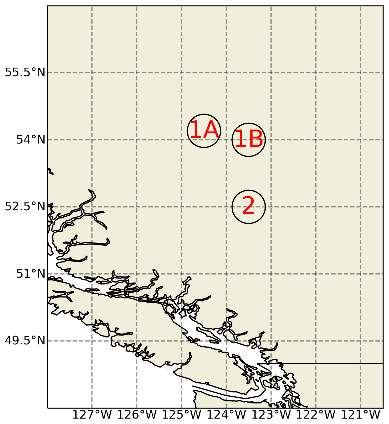
Figure 1Locations of the carbonaceous injections included in the GEOS simulations on 13 August 2017.
2.2 Definition of SWIRL boundaries and data analysis
We define the boundaries of the SWIRL based on the local anomaly of Ertel's potential vorticity (PV) (Ertel, 1942) with respect to the zonal mean at the same altitude and the BrC concentration. We identify the SWIRL as the region where the percent PV anomaly with respect to the PV zonal mean at the same altitude is smaller than −10 % and the mass mixing ratio of BrC is higher than 1.25 µg kg−1. These criteria constrain PV anomalies to those associated with the presence of high carbonaceous aerosol concentrations. In order to obtain smooth SWIRL contours, both the carbonaceous aerosol concentration fields and the PV anomaly fields have been filtered horizontally using a Gaussian filter with a standard deviation of 1∘ in the latitudinal direction and 1.5∘ in the longitudinal direction. We concentrate on model levels higher or equal to 100 hPa, so as to ensure that the detected SWIRL is above the tropopause. The analysis proposed here to track the SWIRL follows the approach of Lestrelin et al. (2021), which uses the Lait PV anomaly (Lait, 1994), along with the ozone concentration anomaly, to locate the SWIRL from ERA5 reanalysis fields. A similar approach was also used by Khaykin et al. (2020) to track the SWIRL from the ANY event.
To investigate the characteristics of the SWIRL, we analyzed the following diagnostic quantities: Ertel's PV, temperature (T), potential temperature (θ), density (ρ), zonal wind speed (U), meridional wind speed (V), vertical wind speed (W), and carbonaceous aerosol (BC and BrC) concentrations. All these quantities are saved on model levels every 6 h, and are presented as absolute fields or as anomalies with respect to their zonal means at the same model level and latitude, unless specified otherwise. The geopotential of the model levels that is present in our discussion is approximated by the mid-layer geometrical height multiplied by the gravitational acceleration g. In our analysis we also used the temperature tendencies due to the diabatic processes resolved by the model (radiation, moist physics, friction, turbulence, and gravity wave drag) and to the dynamics. Additionally, the model calculates the contribution of the aerosol to the temperature tendency due to radiation through two calls to the radiation model, with and without the inclusion of aerosols. In order to better capture the relationship between the SWIRL and its closest surroundings, we restricted our analysis to a region centered on the SWIRL spanning 43.75∘ longitude by 35∘ latitude, and we calculate the diagnostic variables as horizontal averages over the portions of this region inside and outside the SWIRL. The SWIRL geometry was described considering its volume, which is calculated by summing the volumes of the grid cells inside the SWIRL contours over the height of the SWIRL, and its average area, which is calculated by vertically averaging the areas of the SWIRL computed for every layer by summing the areas of the cells' lower boundaries inside the SWIRL selection. The thickness was obtained by considering the height difference between the highest and lowest levels at which the SWIRL was detected.
To visualize and describe the evolution of the bulk SWIRL properties, we considered averages and extremes over the SWIRL volume of our meteorological fields and temperature tendencies.
3.1 SWIRL tracking
In the days following the PNE aerosol injection in the UTLS, the smoke plume drifted eastward and the diabatic self-lofting promoted its vertical movement. A brief description of the smoke transport is available in Appendix A, where we also include a comparison of the plume transport in the free-running and relaxed replay configurations of the GEOS model. This comparison shows how the relaxed replay mode is a good proxy for the observed smoke transport, but has the drawback of damping the effects on the dynamics of the radiative heating of the aerosol. On the other hand, the free-running simulation does not faithfully reproduce the observed smoke transport because the ambient meteorology in the free-running simulation differs from the observed transport. In this work we use the free-running configuration to resolve directly (i.e., with no contribution from reanalysis fields or measurements) the dynamical and thermodynamical impact of the aerosol radiative heating, which is crucial in the formation of the SWIRL.
In our free-running simulations the plume reached 100 hPa on 16 August, consistent with OMPS LP observations (Das et al., 2021), marking the start of the SWIRL detection using the algorithm described in Sect. 2.2. By the end of 18 August the detection algorithm revealed that the bulk of the SWIRL was above the 100 hPa limit, spanning between the levels 100 and 61 hPa. For our analysis, we mark 18 August as the first day of the stratospheric SWIRL. Before this date some signs of SWIRL formation were visible at levels lower than 100 hPa and above the simulated tropopause height (about 150–200 hPa in the days following the injection in the regions corresponding to the plume). We have chosen not to include this initial part in the analysis, since we are interested in the life of the SWIRL when it is well into the stratosphere.
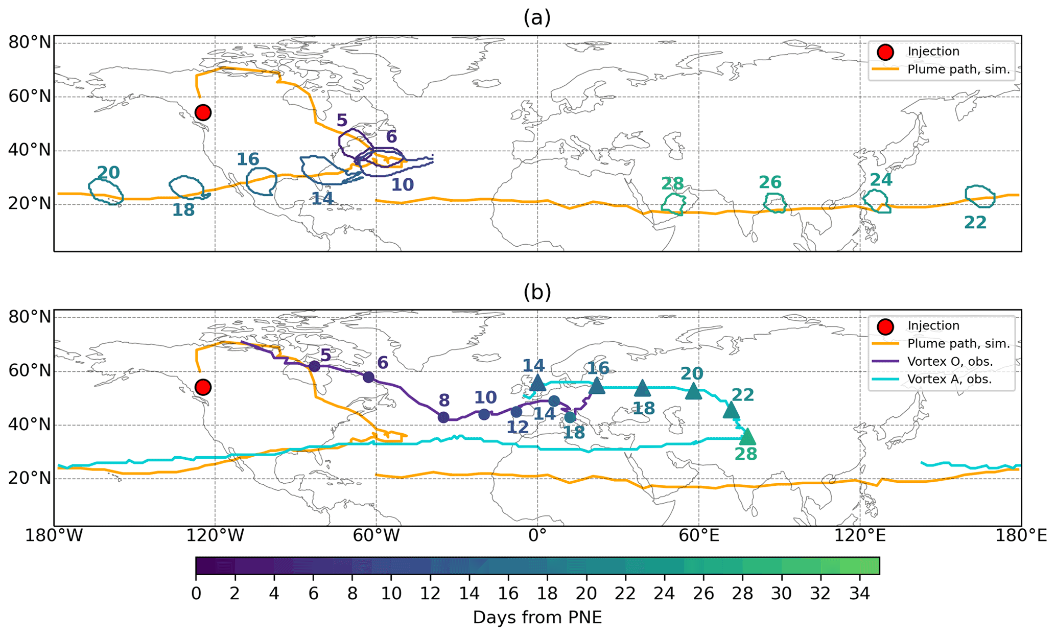
Figure 2Maps showing the path followed by the simulated and observed PNE aerosol plume. The period considered spans from 13 August to 15 October (loss of vortex A in the observations). The orange lines show the evolution in time of the locations of the maximum BrC concentrations in the simulation, considering the regions centered on the SWIRL positions (Sect. 2.2); the red circle over Canada represents the injection location. Panel (a) shows the time evolution of the simulated SWIRL starting on 18 August. The closed contours show the regions where the SWIRL is detected in at least two vertical layers for several selected days. The contours are color-coded and labeled according to the number of days passed since the PNE event. Panel (b) shows paths and timing of the observed vortex O (full circles, dark blue line) and vortex A (full triangles, light blue line) for several selected days corresponding to the ones presented in (a). The full circles and triangles are color-coded and labeled according to the number of days passed since the PNE. The data on the observed stratospheric vortices were kindly provided by Bernard Legras and were obtained tracking the vortices' ozone anomalies in ERA5 fields, as described in Lestrelin et al. (2021).
The SWIRL is first detected by the algorithm over the Atlantic on 18 August (Fig. 2a) and it traveled southeastward until it reached the northern Atlantic. Here it stalled for 7 d (days 6–12 after the PNE, 19–25 August) before starting its westward movement, which eventually brought it to the Arabic peninsula (day 28 after the PNE, 10 September). The next day (11 September, day 29), the SWIRL started losing compactness and that marked the end of its stratospheric lifetime. After this date, the detection algorithm was still able to detect its fragmented remains until at least 16 September, when they reached the Caribbean Sea. The contours of the fragmented SWIRL have not been included in Fig. 2a.
The simulated development of the SWIRL differs from the observed one in several aspects. First, the transport is different, as shown in Fig. 2. The simulated stalling of the vortex on days 6–12 is absent in the observations (Lestrelin et al., 2021), where the vortex moves more quickly eastward. Second, Lestrelin et al. (2021) document the formation of offspring from the initial vortex (vortex O) following its stretching by the ambient meteorology: around 22 August a first splitting of the plume occurs, resulting in the formation of vortex A (light blue line, Fig. 2b) from vortex O (dark blue line, Fig. 2b). Moreover, on 1 September, vortex O split into two vortices (B1 and B2), whose trajectories are not reported here. This splitting is not reproduced by the simulations. Lastly, the simulated SWIRL lasted 25 d overall, which is shorter than in observations Lestrelin et al. (2021), where vortex A remained visible until 15 October. The differences between the simulated and observed development of the SWIRL are due to the underlying meteorology. The generation of offspring vortices and the development of stalling periods are caused by the interaction of the vortex with surrounding meteorological features, such as jets and troughs. Since the underlying meteorology is different in the simulation and observations, its influence on the smoke plume and on the anticyclonic vortices will be different, and we do not expect the evolution of the plume to be the same. Additionally, differences in the amount and properties of the carbonaceous aerosols in the simulated vortex with respect to the observed ones result in differences in its radiative interaction and, therefore, in its evolution.
3.2 Analysis of the SWIRL on 23 August
In this section we describe the structure of the simulated SWIRL on 23 August. On this day the vortex is well into the stratosphere (detected in the model levels between 72 and 43 hPa), with tangential wind speed anomalies of about 10 m s−1, and well organized, with a clear anticyclonic circulation closed around its center.
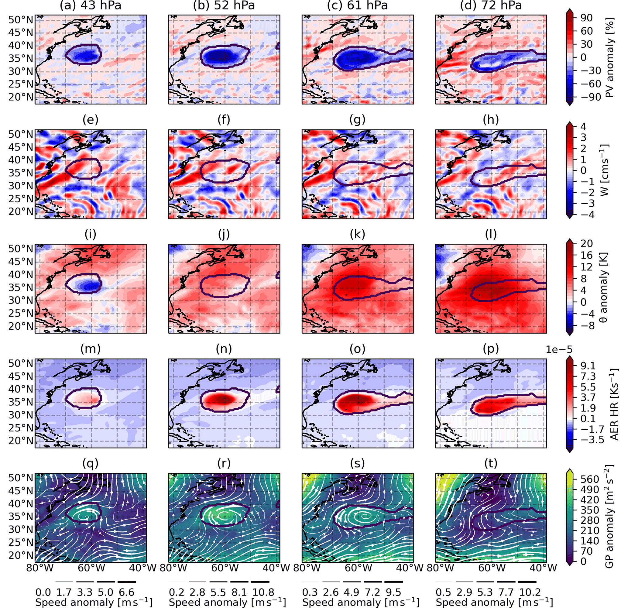
Figure 3Horizontal sections at different heights of the SWIRL on 23 August, 18:00 Z, when the maximum heating occurs. The first to the fourth columns show 43, 52, 61, and 72 hPa altitudes, respectively. The first row (a–d) shows the potential vorticity anomaly [%], the second (e–h), the vertical velocity, the third (i–l), the potential temperature anomaly, the fourth (m–p), the temperature tendency due to radiative heating or cooling of the aerosol, and the fifth row (q–t), the geopotential anomaly (color shades) and the wind field anomaly (white arrows). All anomalies are calculated with respect to the zonal mean. The geopotential anomaly was made positive in the considered region by summing the absolute value of the minimum of the geopotential anomaly to the entire field. This was done for representation purposes. The black contours represent the boundary of the detected SWIRL.
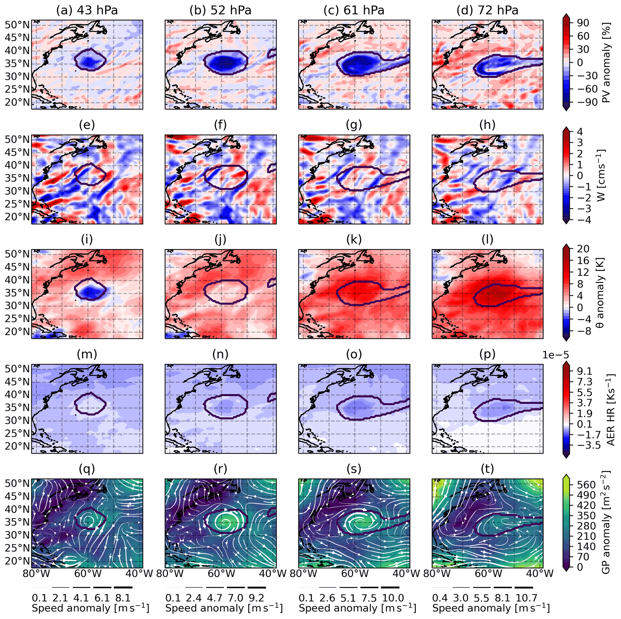
Figure 4Same as Fig. 3, but for 23 August 00:00 Z, when the aerosol is cooling due to the lack of incoming solar radiation.
Inside the borders of the SWIRL lies the deep negative PV anomaly, which indicates the presence of an anticyclone (Figs. 3a–d and 4a–d). Indeed, the horizontal wind anomaly structure of the SWIRL shows an anticyclonic circulation centered over the PV anomaly minimum, with tangential wind magnitudes of about 10 m s−1 (Figs. 3q–t and 4q–t). The magnitude of the tangential wind speed in the SWIRL simulated here is comparable to those presented in the literature for the SWIRL developed after the ANY event (Kablick et al., 2020; Allen et al., 2020). The analysis of the geopotential shows a positive anomaly corresponding to the SWIRL (Figs. 3q–t and 4q–t): this indicates that the effect of the aerosol is to trigger an outward pressure gradient force that, together with Coriolis acceleration, produces the anticyclonic motion of the SWIRL.
The pyroCb aerosol causes a strong internal heating of the SWIRL during daytime (Fig. 3m–p). During nighttime the aerosol does not absorb SW radiation but emits LW radiation, inducing a net cooling of the plume (Fig. 4m–p). Vertical velocities within the SWIRL are comparable to those outside the SWIRL (Fig. 4e–h). From this analysis there is no evidence of an organized structure in the vertical wind field corresponding to the SWIRL and there is no sign of its upward movement. This, however, is expected considering that the vertical displacement of the SWIRL, which can be quantified in hundreds of meters per day, should be driven by a vertical velocity of the order of fractions of cm s−1, which cannot be visible in the noisy vertical velocity background. The lofting of the SWIRL will be made evident later, considering the average of the vertical velocity in the SWIRL (Fig. 7).
While the higher levels of the SWIRL are approximately elliptic, the lowermost levels present a peculiar shape, consisting of an ellipsoid to which a protrusion is attached in the downwind direction. This protrusion can be seen as the tail of the SWIRL, which gradually loses material in time, leaving a trail of air with negative PV anomaly and high aerosol concentration that is classified as SWIRL by our detection method. Such tails have been also observed by Lestrelin et al. (2021).
Another characteristic feature of SWIRLs is the vertical potential temperature anomaly dipole. This is visible considering the maps of potential temperature anomaly (Figs. 3i–l and 4i–l), which indicate a negative anomaly above the center of the SWIRL and a positive anomaly below. As stated by Allen et al. (2020), this signature in the potential temperature is consistent with the vertical expansion of the plume due to the diabatic heating of the aerosol.
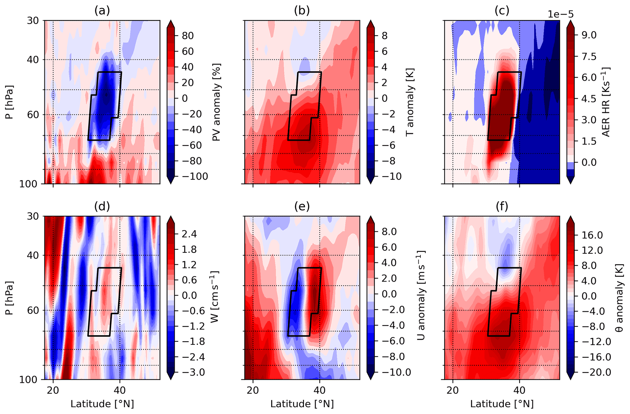
Figure 5Vertical cross section at fixed longitude (−59∘ W) of the SWIRL on 23 August, 18:00 Z. Panel (a) shows the percent relative potential vorticity anomaly, (b) the temperature anomaly, (c) the temperature tendency due to the aerosol heating, (d) the vertical velocity, (e) the zonal wind anomaly, and (f) the potential temperature anomaly. All anomalies are calculated with respect to the zonal mean between −180 and +180∘ longitude.
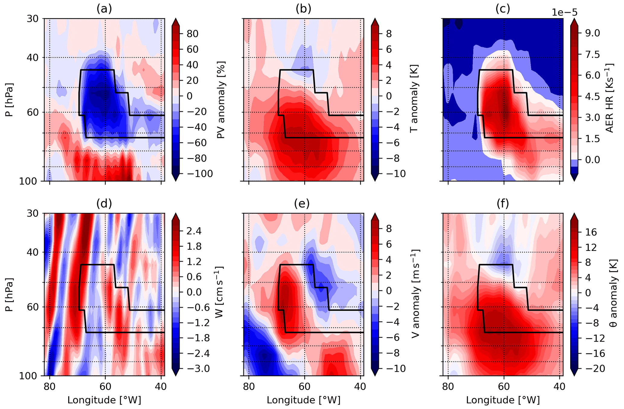
Figure 6Same as Fig. 5 but for a fixed latitude (36∘ N). Panel (e) contains the meridional velocity anomaly.
In the vertical sections of the SWIRL (Figs. 5–6e) a strong anticyclonic motion is visible as well as the vertical structure of the diabatic heating provided by the aerosol (Figs. 5–6c), which is particularly intense in the middle of the SWIRL. The analysis of the meridional wind anomaly curtain (Fig. 6e) reveals also the tilting of the SWIRL, whose axis lies at an angle with respect to the vertical. As described by Allen et al. (2020), the tilting of the vortex is given by the wind shear in the vertical direction. The characteristic vertical temperature and potential temperature anomaly dipoles that characterize SWIRLs are also visible in Figs. 5b–f and 6b–f, with negative anomalies in the upper part of the SWIRL and positive anomalies below. The magnitude of the temperature dipole (10 K) is comparable to that reported for the ANY case (Allen et al., 2020), which reached 15 K. The temperature and potential temperature anomalies extend well below and above the PV anomaly, as also reported in Allen et al. (2020); Lestrelin et al. (2021) and Kablick et al. (2020). As in the horizontal sections, the vertical velocity field does not exhibit any detectable difference between the interior of the SWIRL and its surroundings.
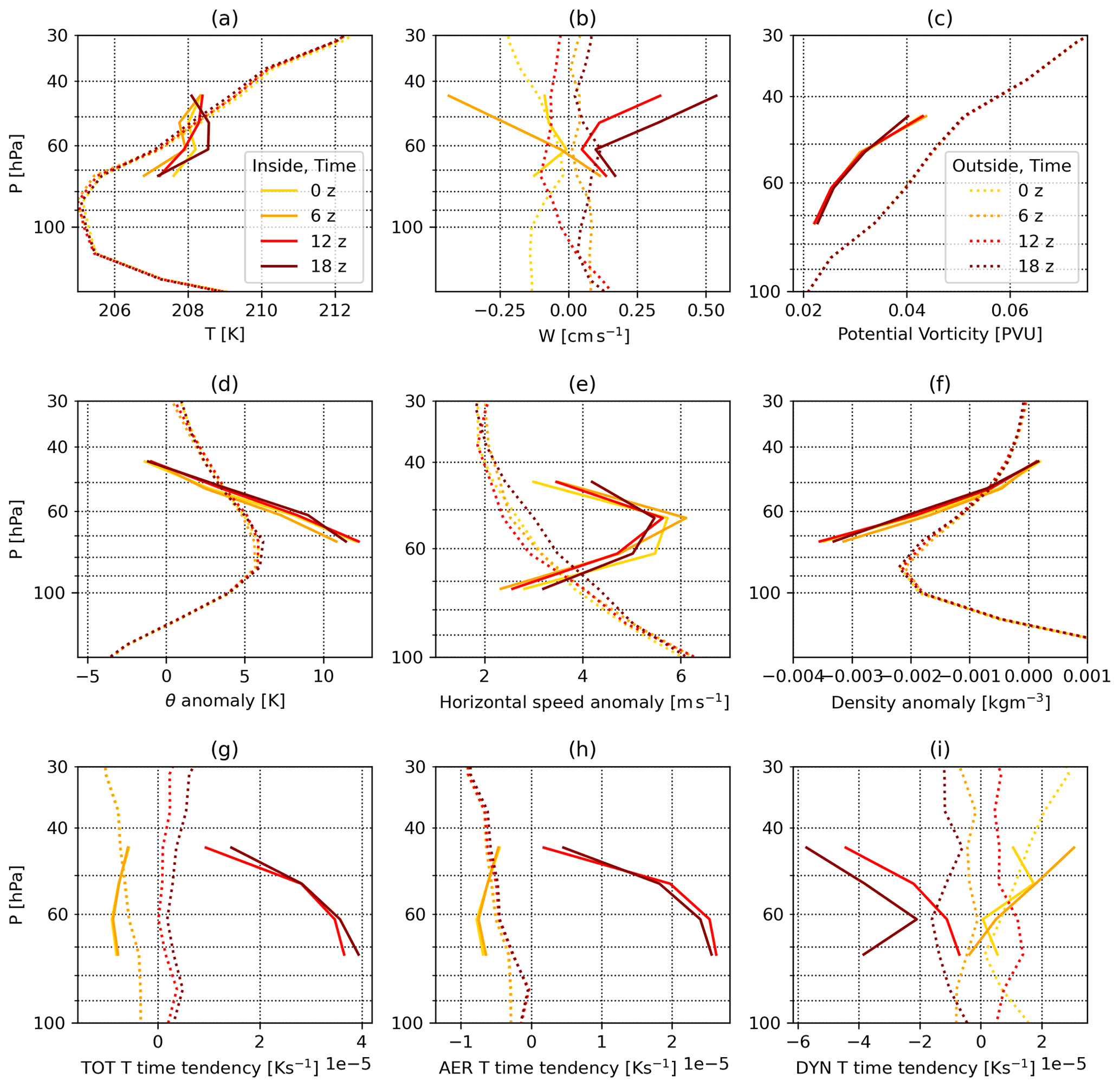
Figure 7Vertical profiles at four different times (00:00–06:00–12:00–18:00 Z) for 23 August. Solid lines represent vertical profiles of the horizontal averages inside the SWIRL selection, while dotted lines represent vertical profiles of the horizontal averages outside the SWIRL selection in a rectangular region 43.75∘ longitude by 35∘ latitude centered on the SWIRL. The panels show (a) absolute temperature, (b) vertical velocity, (c) Ertel's potential vorticity, (d) potential temperature anomaly with respect to the zonal mean, (e) horizontal speed anomaly with respect to the zonal mean, (f) density anomaly, (g) temperature tendency due to diabatic processes, (h) temperature tendency due to the aerosol, and (i) temperature tendency due to the dynamics.
The temperature anomaly dipole shown in Figs. 5b and 6b is reflected in a reduced lapse rate inside the SWIRL compared to the surroundings (Fig. 7a), with the internal temperature profile intersecting the external one roughly in the middle of the SWIRL. The same can be observed in the potential temperature anomaly (Fig. 7d). Figure 7h shows the diurnal heating and nocturnal cooling of the SWIRL due to aerosols and Fig. 7b its resulting vertical motion. The difference in the average vertical velocity between the interior and exterior of the SWIRL is crucial, since it explains how the SWIRL actually moves upward despite being immersed in a noisy vertical velocity field.
The profile of the horizontal wind speed anomaly (Fig. 7e) shows stronger wind speeds in the middle part of the SWIRL; this was visible also in Fig. 3. The reason for this is that the concentrated heating that takes place inside the SWIRL produces a strong rotation which does not interact with the background flow. Indeed, the similarly strong heating taking place at the bottom of the SWIRL (Fig. 7h) does not result in a similarly strong rotation due to the SWIRL interaction with the background flow. This fact is also supported by the shape of the SWIRL, which presents tails in its lower levels caused by the dispersive action of the background flow.
The radiative heating or cooling due to the aerosol is the main factor among the physical diabatic processes (Fig. 7g–i). During the day, the SWIRL is subject to strong diabatic heating, which promotes the vertical motion from buoyancy. The vertical motion is accompanied by the expansion of the SWIRL, which partially compensates for this heating: this is evident in the temperature tendency due to the dynamics (Fig. 7b and i, red and dark red curves). During the night, the opposite situation occurs. The diabatic cooling drives a downward vertical motion of the SWIRL and its subsequent heating due to expansion (Fig. 7b and i, yellow and orange curves). The nocturnal cooling is less intense in absolute value than the diurnal heating. This points toward a net ascent of the SWIRL, given the enhanced intensity of the diurnal lofting with respect to the nocturnal descent (Fig. 7h).
3.3 Evolution in time of the SWIRL properties
The volume of the SWIRL increases until day 10–11 (22–23 August) and then decreases steadily in time (Fig. 8a). The daily modulation of the volume, corresponding to the expansion–compression cycle caused by the diurnal radiative cycle, is visible especially in the first 11–12 d. Accordingly, the calculated radius (Fig. 8b) shows the same time evolution, peaking around day 11 at 700 km. The peak radius of the simulated SWIRL is comparable to the maximum radius of the SWIRL observed following ANY (peaking at 750 km, Allen et al., 2020); instead, the simulated SWIRL is consistently larger in comparison with the main SWIRL observed following PNE, whose horizontal dimensions (diameter) where estimated at 700 km from composite analysis (Lestrelin et al., 2021). After day 28 (11 September) the SWIRL volume increases significantly, following its dispersion and fragmentation. The detection algorithm still categorizes the remains of the plume as SWIRL even thought they lack the characteristic compactness of SWIRLs. This process is also visible in the calculated average radius, with a steep increase after day 28. Moreover, the SWIRL thickness (Fig. 8c) indicates that the SWIRL reaches a maximum thickness of 5 km between day 11 (24 August) and 16 (29 August); before and after this period, the thickness value fluctuates between 3 and 4 km; the magnitude of the SWIRL thickness is comparable to the one observed in the ANY SWIRL, that peaked at 6 km in the moment of its maximum expansion (Allen et al., 2020), and it is also close to the thickness of 3 km of the PNE SWIRL obtained from the composite analysis of Lestrelin et al. (2021). The step-like fluctuations of the SWIRL thickness is due to the vertical resolution of the model at the considered levels, which is around 1 km. The ascent of the simulated SWIRL can be divided in two phases: the steep initial ascent, during which the volume of the SWIRL increases, and a second slower ascent phase, characterized by a decrease in volume of the SWIRL. The potential temperature θ increases approximately linearly (Fig. 8d) during both ascent phases, with a slope of about 10 K d−1 during the first phase and of 6 K d−1 during the second. The ascent speeds are consistent with the observed ones during the ANY SWIRL: in Allen et al. (2020) the ascent speed during the first 27 d of the SWIRL life is estimated at 7.8 and at 5.5 K d−1 afterwards. The potential temperature of the simulated vortex is about 50 K higher than in Lestrelin et al. (2021) (Fig. 8d), possibly because of the faster and more consistent simulated ascent of the plume in the first days following the PNE (see also Appendix A). Despite this offset, between days 5 and 29 from the PNE the ascent rates of the simulated SWIRL are compatible to the rate of vortex O observed by Lestrelin et al. (2021). In the first 11 d of its life, vortex O has an ascent rate of about 9 K d−1, while after its first splitting (formation of vortex A) it rises in the stratosphere at about 4.7 K d−1. These estimates have been obtained with linear fits of the potential temperature curve of vortex O. Before its dissipation 30 d after the PNE, the simulated SWIRL reaches an average potential temperature of 590 K, comparable to the final potential temperature reached by vortex A (570 K) before its loss 60 d after the PNE (Lestrelin et al., 2021). Lastly, the average absolute temperature T within the SWIRL (Fig. 8f) shows little variation in time, with values between 206 and 209 K.
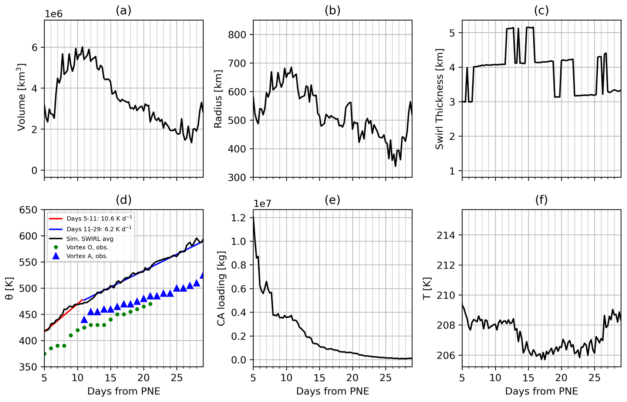
Figure 8Evolution in time of the SWIRL (a) volume, (b) mean radius, (c) thickness, (d) average potential temperature, (e) carbonaceous aerosol loading, and (f) absolute temperature. In (d) the red line shows the result of the linear fit between day 5 and 11 of the potential temperature, while the blue line is between day 11 and day 30. The steepness of the red line is 10.6 K d−1, while for the blue line it is 6.2 K d−1. The green dots and the blue triangles represent the potential temperature of vortices O and A, respectively, obtained using ERA5 meteorological fields in Lestrelin et al. (2021). The data were kindly provided by Bernard Legras.
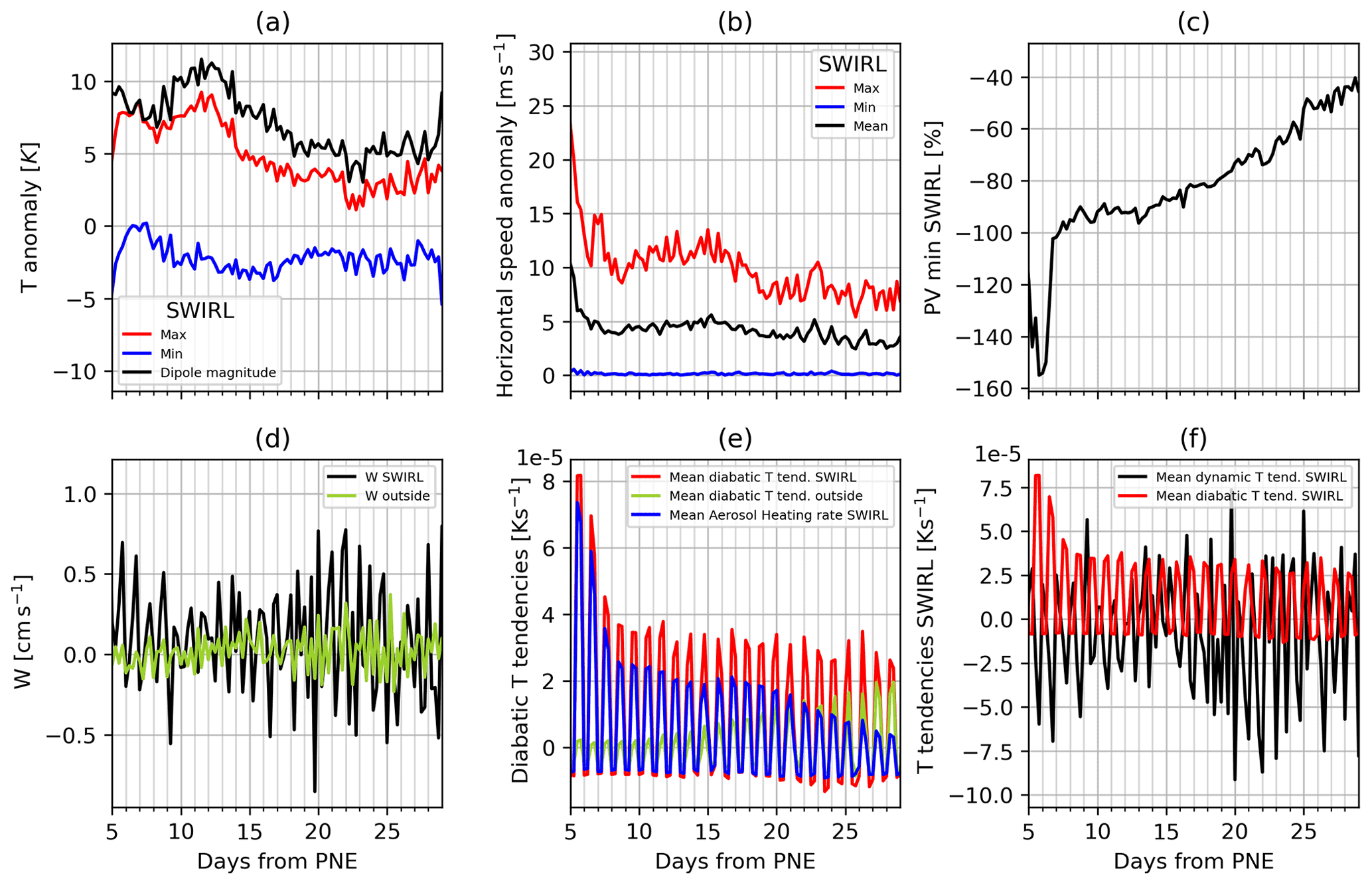
Figure 9Evolution in time of (a) maximum (red line) and minimum (blue line) temperature anomalies inside the SWIRL with respect to the zonal mean; the black line represents the magnitude of the temperature anomaly dipole computed as the distance between the red and blue lines. (b) Maximum (red line), minimum (blue line), and average (black line) speed anomalies with respect to the zonal mean inside the SWIRL (red line). (c) The minimum percent relative Ertel's PV anomaly with respect to the zonal mean inside the SWIRL. (d) The average vertical velocity in the SWIRL (black line) and outside the SWIRL (green line). (e) Average temperature tendency in the SWIRL due to diabatic processes (red line), average temperature tendency due to aerosol inside the SWIRL (blue line), and average temperature tendency outside the SWIRL due to diabatic processes (green line). (f) Averages inside the SWIRL of dynamical (black line) and total diabatic (red line) temperature tendencies. The green lines have been computed as follows: a region centered in the SWIRL of 43.75∘ longitude by 35∘ latitude was selected and the averages were carried out over the portion of this region at the same height of the SWIRL but outside the SWIRL.
The magnitude of the temperature anomaly dipole in the SWIRL is approximately stable until day 10–11 (22–23 August), and then gradually decreases as the SWIRL ages (Fig. 9a). The simulated temperature dipole (peaking at 7 K) is significantly more pronounced than the one calculated for the main PNE SWIRL via composite analysis by Lestrelin et al. (2021) (peaking at 2 K). The maximum horizontal wind speed anomaly in the SWIRL (Fig. 9b) first decreases for 3 d, in the same period in which the radius of the SWIRL increases significantly; then it stabilizes around 12–13 m s−1 before decreasing again after day 15 (28 August) and reaching figures between 6 and 8 m s−1. The same behavior is observed in the average horizontal velocity anomaly that decreases in the first days from 10 to 5 m s−1, then remains constant at 5 m s−1 until day 15, and subsequently decreases gradually reaching 3 m s−1 at the end of the SWIRL lifetime.
The minimum of the PV anomaly (Fig. 9c) abruptly increases at day 6–7 from about −140 % to about −90 % and remains roughly stable until day 11, when it starts increasing at a slower rate. The average vertical velocity of the SWIRL (Fig. 9d) is positive (indicating upwelling) at the end of the daily heating period and negative during the night, with maximum values peaking at 0.7 cm s−1. The average vertical velocity of the SWIRL reaches more pronounced peaks than those of the surroundings, indicated by a green line in Fig. 9d.
The diabatic temperature tendency (Fig. 9e) is initially dominated by the radiative heating of the aerosol. The mean aerosol heating rate within the SWIRL is significantly larger than the average background diabatic temperature tendency until day 22–23 (4–5 September). After this day, the diabatic temperature tendency inside the SWIRL becomes progressively closer to the diabatic temperature tendency outside. The quick loss of coherence of the SWIRL that takes place after day 28 is driven by the loss of this differential heating between its inner region and the surroundings. The dynamical temperature tendency is anticorrelated with the diabatic temperature tendency (Fig. 9f), which is dominated by the aerosol heating, and is directly linked to the vertical velocity of the SWIRL: when the SWIRL is heated by radiation, it rises and expands, meaning that its average vertical velocity is positive and the dynamical temperature tendency is negative. During the night this tendency is reversed along with an average negative vertical velocity. This means that while the SWIRL is cooling, it moves downward while being subject to compression.
Overall, GEOS simulates a SWIRL with intensity and characteristics similar to what was observed after the ANY and PNE events (Lestrelin et al., 2021; Allen et al., 2020). The GEOS-simulated SWIRL has a shorter lifetime than in observations and produces a different trajectory. A key point in maintaining the SWIRL appears to be the difference between the diabatic heating within the SWIRL and the surroundings. This depends on the SWIRL's aerosol loading and its radiative properties, as well as the local meteorology and the location of the vortex. Therefore, a role in determining the development of the SWIRL must be played by the specific meteorological conditions after the event, which are not expected to be reproduced in a free-running simulation. A whole ensemble of free-running simulations should be used to analyze the importance of specific background meteorological conditions on the formation and dissipation of the SWIRL, as well as the interaction of aerosol heating and background conditions in the initial and final stage of the SWIRL lifetime.
Despite being able to reproduce many characteristics observed in SWIRLs, the configuration of the GEOS model might impact the results. First, the vertical resolution at the stratospheric altitudes analyzed here is about 1 km. A finer resolution could impact the vertical ascent, as clear in the step-wise behavior of the SWIRL thickness visible in Fig. 8. Additionally, the GOCART aerosol module includes a parameterization of the transformation of carbonaceous particles from hydrophobic to hydrophilic and the subsequent hygroscopic growth of hygrophilic particles, but does not include changes in optical properties due to coagulation of aerosols, condensation of gaseous material, or the transfer from external to internal mixture. Lastly, GOCART assumes that BC and BrC aerosols are spherical. Changes in depolarization ratio (both in space and time) as shown in Christian et al. (2019), or fractal structures such as in Yu et al. (2019), are not simulated. Since (Yu et al., 2019) showed that fractal structures are more absorbing at visible wavelengths, the radiative impact that we simulate might be underestimated. This might explain the shorter SWIRL lifetime in our simulations than in observations.
In this work, we present how the GEOS CCM is able to reproduce a SWIRL, i.e., a stratospheric aerosol-induced anticyclone. Previous studies used reanalyses and observations to characterize the SWIRLs generated by the PNE (Lestrelin et al., 2021) and ANY (Allen et al., 2020; Kablick et al., 2020; Khaykin et al., 2020) events. The simulations presented here reproduce several of their findings, and in particular the structures of the anomalies characterizing the SWIRLs. The use of a free-running model with aerosol–radiation coupling allows us for the first time to resolve the role that the aerosol radiative interaction plays in the development of the SWIRL, as well as to characterize the diurnal cycle of the SWIRL and associated transport effects. The presence of the heating of the aerosol is crucial, and Khaykin et al. (2020) showed that, without this contribution, SWIRLs dissipate in around 6–7 d.
In this work, the simulated SWIRL is first recognized by using a simple detection algorithm, based on Ertel's PV anomaly and on the BrC concentration. The analysis of the SWIRL is carried out by considering its structure on 23 August and then by evaluating how its bulk properties evolved during its lifetime. This analysis shows that the simulated anticyclonic disturbance reproduces the magnitudes of the anomalies of the observed ones; for instance, the magnitude of the flow of the anticyclone is about 10 m s−1, which is close to the magnitude of the flow in the SWIRL observed following ANY (Allen et al., 2020). The same is true for the magnitude of the temperature anomaly dipole, which is observed together with a steeper lapse rate inside the SWIRL than in the surroundings. We also show that the anticyclonic circulation is maintained by a pressure gradient force, triggered by a positive anomaly of the geopotential of the isobaric levels. This enhanced pressure in the center of the SWIRL is given by the diabatic heating of the aerosol, which also leads to the expansion–compression cycle that the SWIRL undergoes and its consequent net diabatic lofting.
The diurnal cycle of the SWIRL is modulated by the daily radiation cycle. During daytime, the aerosol heats up the atmosphere through the absorption of solar radiation. This triggers a radial expansion of the plume and a consequent vertical motion due to buoyancy. The expansion of the plume is also accompanied by its dynamical cooling, which effectively counteracts the diabatic heating provided by the aerosol; as a result, the overall process is almost isothermal.
During the night, when the plume cools down radiatively, the process is inverted, and the SWIRL moves downward. The upward daytime motion is more pronounced than the nighttime one, leading to a net ascension of the plume. The analysis of the evolution of the radius and volume of the SWIRL during its lifetime reveals this daily expansion–compression cycle of the SWIRL.
In conclusion, this work shows that free-running simulations with a chemistry climate model such as GEOS are suitable for studying the formation and development of stratospheric vortices following large injections of carbonaceous aerosols in the UTLS by pyroCb clouds. Indeed, despite the limitations of the configuration and of the models itself, we were able to exploit them to reproduce such an event and to study several dynamical and thermodynamical features of SWIRLs. Several future developments of this work are possible: for example, model simulations with higher vertical resolution could help in determining more accurately the vertical structure of the vortex. Also, an ensemble of simulations such as the ones proposed here could help in better understanding the mechanisms behind the generation, maintenance, and collapse of the vortex.
Here, we compare the transport of the aerosol in the free-running and replay configurations of the GEOS model. The replay simulations presented here are described in depth in Das et al. (2021), and were performed using a relaxed replay configuration.
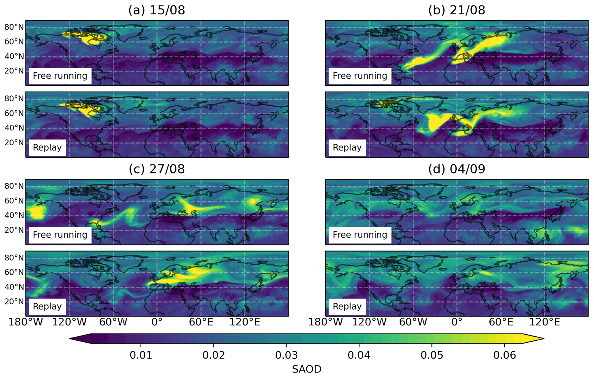
Figure A1Comparison of the zonal mean stratospheric aerosol optical thickness (SAOD) at 550 nm from the free-running and replay simulations for 4 different days in the month following the PNE.

Figure A2Time evolution of the horizontal average over the Northern Hemisphere of the 550 nm extinction coefficient of carbonaceous aerosols.
Following the injection from the PNE, the aerosol released in UTLS started its journey in the stratosphere. The diabatic self-lofting promoted the gradual ascension of the plume while it was advected and dispersed by the large-scale circulation.
The horizontal transport of aerosol is visualized considering maps of SAOD (Stratospheric Aerosol Optical Depth) at 550 nm (Fig. A1). The SAOD is calculated summing the simulated extinction coefficients fields due to the presence of BC and BrC, and vertically integrating them from the tropopause up to the model's top of the atmosphere. The computation of the SAOD has been carried out both for the free-running and replay simulations. As shown in Das et al. (2021), the latter capture well the aerosol transport as observed by OMPS LP; thus, the replay simulation is used here as a reference of the actual aerosol transport.
In the first 2–3 d following the injection, the aerosol is advected and gradually dispersed by the wind field in the UTLS, which moves the plume toward the Atlantic both in the free-running and replay simulations (Fig. A1a); at this stage the difference is limited between the different simulations.
As time passes, the free-running simulation begins to significantly differ from the one in replay configuration (Fig. A1d). Of particular interest during this phase is the splitting of a portion of the plume that can be observed in the free-running simulation around day 11 (24 August 2017) above the northern Atlantic Ocean (Fig. A1, compare panel b with c). After this event, a section of the plume reaches lower latitudes and starts moving toward the Gulf of Mexico.
This southern part of the aerosol plume exhibits interesting properties such as the confinement of the plume itself and its resilience against the disruption operated by the background flow. This portion of the plume generated the SWIRL, which is presented in this article. The splitting of the plume does not occur in the replay configuration, in which the bulk of the aerosol reaches Europe.
In order to compare the vertical displacement in time of the plume, we consider the time evolution of the horizontal average over the Northern Hemisphere of the extinction coefficient due to carbonaceous aerosols at 550 nm (Fig. A2), which reveals a fast ascent of the aerosol plume in the first days following the injection. Comparing the free-running with the replay configurations it is evident that in the former the vertical transport is more pronounced: in the free-running simulation the aerosol that reaches 100 hPa in 5 d is consistently more than in the replay simulation. Only from days 9–10 do we find comparable extinction coefficients above 100 hPa in the replay simulation. This difference in the ascent rate in the replay and free-running configurations could be given by the different background meteorology. Also, in the free-running configuration the model's physics is free from the observational constraints, so that the aerosol diabatic heating can have a direct impact on it; instead in the replay configuration the action of the aerosol in the dynamics might be dampened by the replay procedure itself. However, caution is needed when exploring this argument, since we have a single free-running simulation; the study of an ensemble of free-running simulations might be the correct instrument with which to better quantify and explain the differences in the diabatic self-lofting between the replay and free-running simulations.
The GEOS model is available from an externally accessible subversion software repository, whose details are provided at https://gmao.gsfc.nasa.gov/GEOS_systems/geos5_access.php (NASA, 2022).
The dataset used to obtain the results presented in this article is available for download in the online repository “GEOS CCM free-running simulation data of the Pacific-Northwest pyrocumulonimbus Event-like aerosol injection, SWIRL selection”, https://doi.org/10.5281/zenodo.6366106 (Doglioni, 2022).
PRC and SD designed the modeling approach and performed the simulations. GD performed the data analysis and analyzed the results under the supervision of VA and DZ. GD wrote the manuscript with VA and DZ. All the authors reviewed the manuscript before the submission.
The contact author has declared that none of the authors has any competing interests.
Publisher's note: Copernicus Publications remains neutral with regard to jurisdictional claims in published maps and institutional affiliations.
We would like to acknowledge the NASA Earth Science Division and GEOS model developmental efforts at GMAO for their support and the NASA MAP funding under the GEOS-CCM project (CCM Workpackage; program manager David Considine). Sampa Das's research at NASA GSFC for this effort was supported by an appointment to the NASA Postdoctoral Program (NPP), administered by the Universities Space Research Association under contract with NASA. The computing resources supporting the simulations shown in this work were provided by the NASA High-End Computing (HEC) Program through the NASA Center for Climate Simulation (NCCS) at the Goddard Space Flight Center.
We would also like to acknowledge the Department of Civil, Mechanical and Environmental Engineering of the University of Trento for the financial support given to Giorgio Doglioni during the development of this paper as a graduate student grant.
We also acknowledge the Center Agriculture, Food Environment of the University of Trento and the startup Hypermeteo for funding the PhD scholarship of Giorgio Doglioni, during which this work was finalized.
We also thank Bernard Legras for kindly providing the data on the vortices observed following the PNE, described in Lestrelin et al. (2021).
This paper was edited by Peter Haynes and reviewed by two anonymous referees.
Allen, D. R., Fromm, M. D., Kablick III, G. P., and Nedoluha, G. E.: Smoke with Induced Rotation and Lofting (SWIRL) in the Stratosphere, J. Atmos. Sci., 77, 4297–4316, https://doi.org/10.1175/JAS-D-20-0131.1, 2020. a, b, c, d, e, f, g, h, i, j, k, l, m, n, o
Baars, H., Ansmann, A., Ohneiser, K., Haarig, M., Engelmann, R., Althausen, D., Hanssen, I., Gausa, M., Pietruczuk, A., Szkop, A., Stachlewska, I. S., Wang, D., Reichardt, J., Skupin, A., Mattis, I., Trickl, T., Vogelmann, H., Navas-Guzmán, F., Haefele, A., Acheson, K., Ruth, A. A., Tatarov, B., Müller, D., Hu, Q., Podvin, T., Goloub, P., Veselovskii, I., Pietras, C., Haeffelin, M., Fréville, P., Sicard, M., Comerón, A., Fernández García, A. J., Molero Menéndez, F., Córdoba-Jabonero, C., Guerrero-Rascado, J. L., Alados-Arboledas, L., Bortoli, D., Costa, M. J., Dionisi, D., Liberti, G. L., Wang, X., Sannino, A., Papagiannopoulos, N., Boselli, A., Mona, L., D'Amico, G., Romano, S., Perrone, M. R., Belegante, L., Nicolae, D., Grigorov, I., Gialitaki, A., Amiridis, V., Soupiona, O., Papayannis, A., Mamouri, R.-E., Nisantzi, A., Heese, B., Hofer, J., Schechner, Y. Y., Wandinger, U., and Pappalardo, G.: The unprecedented 2017–2018 stratospheric smoke event: decay phase and aerosol properties observed with the EARLINET, Atmos. Chem. Phys., 19, 15183–15198, https://doi.org/10.5194/acp-19-15183-2019, 2019. a
Bourassa, A. E., Rieger, L. A., Zawada, D. J., Khaykin, S., Thomason, L. W., and Degenstein, D. A.: Satellite Limb Observations of Unprecedented Forest Fire Aerosol in the Stratosphere, J. Geophys. Res.-Atmos., 124, 9510–9519, https://doi.org/10.1029/2019JD030607, 2019. a, b
Chin, M., Ginoux, P., Kinne, S., Torres, O., Holben, B. N., Duncan, B. N., Martin, R. V., Logan, J. A., Higurashi, A., and Nakajima, T.: Tropospheric Aerosol Optical Thickness from the GOCART Model and Comparisons with Satellite and Sun Photometer Measurements, J. Atmos. Sci., 59, 461–483, https://doi.org/10.1175/1520-0469(2002)059<0461:TAOTFT>2.0.CO;2, 2002. a
Chin, M., Diehl, T., Dubovik, O., Eck, T. F., Holben, B. N., Sinyuk, A., and Streets, D. G.: Light absorption by pollution, dust, and biomass burning aerosols: a global model study and evaluation with AERONET measurements, Ann. Geophys., 27, 3439–3464, https://doi.org/10.5194/angeo-27-3439-2009, 2009. a
Christian, K., Wang, J., Ge, C., Peterson, D., Hyer, E., Yorks, J., and McGill, M.: Radiative Forcing and Stratospheric Warming of Pyrocumulonimbus Smoke Aerosols: First Modeling Results With Multisensor (EPIC, CALIPSO, and CATS) Views from Space, Geophys. Res. Lett., 46, 10061–10071, https://doi.org/10.1029/2019GL082360, 2019. a, b, c
Colarco, P., da Silva, A., Chin, M., and Diehl, T.: Online simulations of global aerosol distributions in the NASA GEOS-4 model and comparisons to satellite and ground-based aerosol optical depth, J. Geophys. Res.-Atmos., 115, D14207, https://doi.org/10.1029/2009JD012820, 2010. a
Colarco, P. R., Nowottnick, E. P., Randles, C. A., Yi, B., Yang, P., Kim, K.-M., Smith, J. A., and Bardeen, C. G.: Impact of radiatively interactive dust aerosols in the NASA GEOS-5 climate model: Sensitivity to dust particle shape and refractive index, J. Geophys. Res.-Atmos., 119, 753–786, https://doi.org/10.1002/2013JD020046, 2014. a
Colarco, P. R., Gassó, S., Ahn, C., Buchard, V., da Silva, A. M., and Torres, O.: Simulation of the Ozone Monitoring Instrument aerosol index using the NASA Goddard Earth Observing System aerosol reanalysis products, Atmos. Meas. Tech., 10, 4121–4134, https://doi.org/10.5194/amt-10-4121-2017, 2017. a
Considine, D. B., Douglass, A. R., Connell, P. S., Kinnison, D. E., and Rotman, D. A.: A polar stratospheric cloud parameterization for the global modeling initiative three-dimensional model and its response to stratospheric aircraft, J. Geophys. Res.-Atmos., 105, 3955–3973, https://doi.org/10.1029/1999JD900932, 2000. a
Das, S., Colarco, P. R., Oman, L. D., Taha, G., and Torres, O.: The long-term transport and radiative impacts of the 2017 British Columbia pyrocumulonimbus smoke aerosols in the stratosphere, Atmos. Chem. Phys., 21, 12069–12090, https://doi.org/10.5194/acp-21-12069-2021, 2021. a, b, c, d, e, f, g, h, i, j, k, l, m
de Laat, A. T. J., Stein Zweers, D. C., Boers, R., and Tuinder, O. N. E.: A solar escalator: Observational evidence of the self-lifting of smoke and aerosols by absorption of solar radiation in the February 2009 Australian Black Saturday plume, J. Geophys. Res.-Atmos., 117, D04204, https://doi.org/10.1029/2011JD017016, 2012. a
Ditas, J., Ma, N., Zhang, Y., Assmann, D., Neumaier, M., Riede, H., Karu, E., Williams, J., Scharffe, D., Wang, Q., Saturno, J., Schwarz, J. P., Katich, J. M., McMeeking, G. R., Zahn, A., Hermann, M., Brenninkmeijer, C. A. M., Andreae, M. O., Pöschl, U., Su, H., and Cheng, Y.: Strong impact of wildfires on the abundance and aging of black carbon in the lowermost stratosphere, P. Natl. Acad. Sci. USA, 115, E11595–E11603, https://doi.org/10.1073/pnas.1806868115, 2018. a
Doglioni, G.: GEOS CCM free-running simulation data of the Pacific-Northwest pyrocumulonimbus Event-like aerosol injection, SWIRL selection, Zenodo [data set], https://doi.org/10.5281/zenodo.6366106, 2022. a
Douglass, A. R. and Kawa, S. R.: Contrast between 1992 and 1997 high-latitude spring Halogen Occultation Experiment observations of lower stratospheric HCl, J. Geophys. Res.-Atmos., 104, 18739–18754, https://doi.org/10.1029/1999JD900281, 1999. a
Ertel, H.: Ein neuer hydrodynamischer Erhaltungssatz, Naturwissenschaften, 30, 543–544, https://doi.org/10.1007/BF01475602, 1942. a
Fromm, M., Alfred, J., Hoppel, K., Hornstein, J., Bevilacqua, R., Shettle, E., Servranckx, R., Li, Z., and Stocks, B.: Observations of boreal forest fire smoke in the stratosphere by POAM III, SAGE II, and lidar in 1998, Geophys. Res. Lett., 27, 1407–1410, https://doi.org/10.1029/1999GL011200, 2000. a
Fromm, M., Lindsey, D., Servranckx, R., Yue, G., Trickl, T., Sica, R., Doucet, P., and Godin-Beekmann, S.: The Untold Story of Pyrocumulonimbus, B. Am. Meteorol. Soc., 91, 1193–1210, https://doi.org/10.1175/2010BAMS3004.1, 2010. a, b
Fromm, M. D., Kablick, G. P., Peterson, D. A., Kahn, R. A., Flower, V. J. B., and Seftor, C. J.: Quantifying the Source Term and Uniqueness of the August 12, 2017 Pacific Northwest PyroCb Event, J. Geophys. Res.-Atmos., 126, e2021JD034928, https://doi.org/10.1029/2021JD034928, 2021. a
Gelaro, R., McCarty, W., Suárez, M. J., Todling, R., Molod, A., Takacs, L., Randles, C. A., Darmenov, A., Bosilovich, M. G., Reichle, R., Wargan, K., Coy, L., Cullather, R., Draper, C., Akella, S., Buchard, V., Conaty, A., da Silva, A. M., Gu, W., Kim, G.-K., Koster, R., Lucchesi, R., Merkova, D., Nielsen, J. E., Partyka, G., Pawson, S., Putman, W., Rienecker, M., Schubert, S. D., Sienkiewicz, M., and Zhao, B.: The Modern-Era Retrospective Analysis for Research and Applications, Version 2 (MERRA-2), J. Climate, 30, 5419–5454, https://doi.org/10.1175/JCLI-D-16-0758.1, 2017. a
Hess, M., Koepke, P., and Schult, I.: Optical Properties of Aerosols and Clouds: The Software Package OPAC, B. Am. Meteorol. Soc., 79, 831–844, https://doi.org/10.1175/1520-0477(1998)079<0831:OPOAAC>2.0.CO;2, 1998. a
Kablick III, G. P., Allen, D. R., Fromm, M. D., and Nedoluha, G. E.: Australian PyroCb Smoke Generates Synoptic-Scale Stratospheric Anticyclones, Geophys. Res. Lett., 47, e2020GL088101, https://doi.org/10.1029/2020GL088101, 2020. a, b, c, d
Khaykin, S. M., Godin-Beekmann, S., Hauchecorne, A., Pelon, J., Ravetta, F., and Keckhut, P.: Stratospheric Smoke With Unprecedentedly High Backscatter Observed by Lidars Above Southern France, Geophys. Res. Lett., 45, 1639–1646, https://doi.org/10.1002/2017GL076763, 2018. a
Khaykin, S., Legras, B., Bucci, S., Sellitto, P., Isaksen, L., Tencé, F., Bekki, S., Bourassa, A., Rieger, L., Zawada, D., Jumelet, J., and Godin-Beekmann, S.: The 2019/20 Australian wildfires generated a persistent smoke-charged vortex rising up to 35 km altitude, Communications Earth & Environment, 1, 22, https://doi.org/10.1038/s43247-020-00022-5, 2020. a, b, c, d, e, f, g
Kloss, C., Berthet, G., Sellitto, P., Ploeger, F., Bucci, S., Khaykin, S., Jégou, F., Taha, G., Thomason, L. W., Barret, B., Le Flochmoen, E., von Hobe, M., Bossolasco, A., Bègue, N., and Legras, B.: Transport of the 2017 Canadian wildfire plume to the tropics via the Asian monsoon circulation, Atmos. Chem. Phys., 19, 13547–13567, https://doi.org/10.5194/acp-19-13547-2019, 2019. a
Lait, L. R.: An Alternative Form for Potential Vorticity, J. Atmos. Sci., 51, 1754–1759, https://doi.org/10.1175/1520-0469(1994)051<1754:AAFFPV>2.0.CO;2, 1994. a
Lestrelin, H., Legras, B., Podglajen, A., and Salihoglu, M.: Smoke-charged vortices in the stratosphere generated by wildfires and their behaviour in both hemispheres: comparing Australia 2020 to Canada 2017, Atmos. Chem. Phys., 21, 7113–7134, https://doi.org/10.5194/acp-21-7113-2021, 2021. a, b, c, d, e, f, g, h, i, j, k, l, m, n, o, p, q, r, s, t
Molod, A., Takacs, L., Suarez, M., and Bacmeister, J.: Development of the GEOS-5 atmospheric general circulation model: evolution from MERRA to MERRA2, Geosci. Model Dev., 8, 1339–1356, https://doi.org/10.5194/gmd-8-1339-2015, 2015. a
NASA: GMAO, GEOS model, NASA [model], https://gmao.gsfc.nasa.gov/GEOS_systems/geos5_access.php, last access: 22 August 2022. a
Peterson, D. A., Hyer, E. J., Campbell, J. R., Solbrig, J. E., and Fromm, M. D.: A Conceptual Model for Development of Intense Pyrocumulonimbus in Western North America, Mon. Weather Rev., 145, 2235–2255, https://doi.org/10.1175/MWR-D-16-0232.1, 2017. a
Peterson, D., Campbell, J., and Hyer, E. E. A.: Wildfire-driven thunderstorms cause a volcano-like stratospheric injection of smoke, npj Climate and Atmospheric Science, 1, 30, 587–590, https://doi.org/10.1038/s41612-018-0039-3, 2018. a, b, c, d
Peterson, D. A., Fromm, M. D., McRae, R. H. D., Campbell, J. R., Hyer, E. J., Taha, G., Camacho, C. P., Kablick, G. P., Schmidt, C. C., and DeLand, M. T.: Australia's Black Summer pyrocumulonimbus super outbreak reveals potential for increasingly extreme stratospheric smoke events, npj Climate and Atmospheric Science, 4, 38, https://doi.org/10.1038/s41612-021-00192-9, 2021. a
Rienecker, M., Suarez, M., Todling, R., Bacmeister, J., Takacs, L., Liu, H., Gu, W., Sienkiewicz, M., Koster, R., Gelaro, R., Stajner, I., and Nielsen, J.: The GEOS-5 Data Assimilation System – Documentation of Versions 5.0.1, 5.1.0, and 5.2.0, Tech. rep., Global Modelling and Assimilation Office (GMAO), NASA, https://gmao.gsfc.nasa.gov/pubs/docs/tm27.pdf (last access: 22 August 2022), 2008. a, b
Torres, O., Bhartia, P. K., Taha, G., Jethva, H., Das, S., Colarco, P., Krotkov, N., Omar, A., and Ahn, C.: Stratospheric Injection of Massive Smoke Plume From Canadian Boreal Fires in 2017 as Seen by DSCOVR-EPIC, CALIOP, and OMPS-LP Observations, J. Geophys. Res.-Atmos., 125, e2020JD032579, https://doi.org/10.1029/2020JD032579, 2020. a, b, c, d, e, f
Wiedinmyer, C., Akagi, S. K., Yokelson, R. J., Emmons, L. K., Al-Saadi, J. A., Orlando, J. J., and Soja, A. J.: The Fire INventory from NCAR (FINN): a high resolution global model to estimate the emissions from open burning, Geosci. Model Dev., 4, 625–641, https://doi.org/10.5194/gmd-4-625-2011, 2011. a
Yu, P., Toon, O. B., Bardeen, C. G., Zhu, Y., Rosenlof, K. H., Portmann, R. W., Thornberry, T. D., Gao, R.-S., Davis, S. M., Wolf, E. T., de Gouw, J., Peterson, D. A., Fromm, M. D., and Robock, A.: Black carbon lofts wildfire smoke high into the stratosphere to form a persistent plume, Science, 365, 587–590, https://doi.org/10.1126/science.aax1748, 2019. a, b, c, d, e