the Creative Commons Attribution 4.0 License.
the Creative Commons Attribution 4.0 License.
 | 24 Jan 2022
Four years of global carbon cycle observed from the Orbiting Carbon Observatory 2 (OCO-2) version 9 and in situ data and comparison to OCO-2 version 7
Sean Crowell
Andrew Schuh
David F. Baker
Chris O'Dell
Andrew R. Jacobson
Frédéric Chevallier
Junjie Liu
Annmarie Eldering
David Crisp
Feng Deng
Brad Weir
Sourish Basu
Matthew S. Johnson
Sajeev Philip
Ian Baker
The Orbiting Carbon Observatory 2 (OCO-2) satellite has been providing information to estimate carbon dioxide (CO2) fluxes at global and regional scales since 2014 through the combination of CO2 retrievals with top–down atmospheric inversion methods. Column average CO2 dry-air mole fraction retrievals have been constantly improved. A bias correction has been applied in the OCO-2 version 9 retrievals compared to the previous OCO-2 version 7r improving data accuracy and coverage. We study an ensemble of 10 atmospheric inversions all characterized by different transport models, data assimilation algorithms, and prior fluxes using first OCO-2 v7 in 2015–2016 and then OCO-2 version 9 land observations for the longer period 2015–2018. Inversions assimilating in situ (IS) measurements have also been used to provide a baseline against which the satellite-driven results are compared. The time series at different scales (going from global to regional scales) of the models emissions are analyzed and compared to each experiment using either OCO-2 or IS data. We then evaluate the inversion ensemble based on the dataset from the Total Carbon Column Observing Network (TCCON), aircraft, and in situ observations, all independent from assimilated data. While we find a similar constraint of global total carbon emissions between the ensemble spread using IS and both OCO-2 retrievals, differences between the two retrieval versions appear over regional scales and particularly in tropical Africa. A difference in the carbon budget between v7 and v9 is found over this region, which seems to show the impact of corrections applied in retrievals. However, the lack of data in the tropics limits our conclusions, and the estimation of carbon emissions over tropical Africa require further analysis.
- Article
(7104 KB) - Full-text XML
- BibTeX
- EndNote


Understanding the global carbon cycle and how quickly the planet warms in response to human activities is becoming a global priority. CO2 is a key driver of global warming, and its dynamics can be explored with a variety of CO2 measurements. Ground-based (in situ) data, while highly precise and accurate, are distributed very sparsely over the globe (Ciais et al., 2013). Space-based CO2 retrievals, on the other hand, allow comprehensive spatial coverage across the globe, particularly over regions with few surface observations, such as the tropics. Furthermore, the number of satellites observing atmospheric CO2 has rapidly grown over the past decade, e.g., the Greenhouse Gases Observing Satellite (GOSAT/GOSAT2 Kuze et al., 2009; Nakajima et al., 2012) and the Orbiting Carbon Observatory (OCO-2/OCO-3 Crisp et al., 2017; Eldering et al., 2017).
The rise in CO2 concentration at a global scale has motivated the drive towards a better understanding of the global surface fluxes of carbon (World Meteorological Organisation, 2020). In order to understand the different processes involved in the carbon cycle, such as uptake or release of CO2 by the oceans and the land biosphere, and hence be able to predict future climate change, we need accurate emissions estimates and an improved understanding of natural CO2 emissions and uptakes. Top–down atmospheric inversion approaches that couple atmospheric observations of CO2 with chemistry (atmospheric) transport models (CTMs) have been widely used to estimate CO2 fluxes (Ciais et al., 2010; Peylin et al., 2013; Basu et al., 2013; Wang et al., 2018; Crowell et al., 2019). This is in contrast to “bottom–up” methods, which often use a mechanistic understanding of the carbon cycle, e.g., soil dynamics, photosynthesis, decomposition processes, and steady-state ocean–atmospheric chemical exchange, to predict land and ocean–atmospheric exchange and hence atmospheric CO2 concentrations. While the mechanistic underpinnings of these models are attractive, there is no guarantee that the resulting atmospheric exchange of CO2 will bear any similarity to reality. By contrast, the “top–down” approach often uses a “bottom–up” model output as a starting guess and then optimizes atmospheric exchange to agree with atmospheric observations.
Formal uncertainties of top–down approaches can be attributed to the errors in the observations assimilated, i.e., “observation” errors, and to errors in the starting guess from mechanistic models. However, past studies have also shown that top–down estimates can be sensitive to errors in the modeled atmospheric transport as well as in choices related to the optimization technique (Chevallier et al., 2010; Houweling et al., 2015; Basu et al., 2018; Schuh et al., 2019), uncertainties which are difficult if not impossible to characterize formally in any one atmospheric inversion scheme. This shortcoming was the motivation for the OCO-2 Model Inter-comparison Project (MIP), whose goal was to (1) study the impact of assimilating OCO-2 retrieval data into several atmospheric inversion models and (2) provide an overall ensemble spread of the model emissions characterizing most sources of known uncertainty. In addition to its primary goal of assimilating OCO-2 retrievals, MIP modelers also assimilate in situ data, a practice which has a long and documented history (Enting and Newsam, 1990; Enting, 2002; Gurney et al., 2002; Rayner et al., 2014). In the first iteration of the MIP project (the “v7 MIP”), OCO-2 version 7r land observations were used and analyzed for the 2015–2016 period (Crowell et al., 2019). In that study, the authors found good agreement between in situ and satellite inversions at the global scale. However, differences appeared at smaller regional scales, particularly over the tropics in areas such as northern Africa, where stronger sources were observed with the OCO-2 inversions than with the in situ inversions. The authors concluded that the differences over the tropics, besides being due to better observability in a region with few in situ observations, could be due to the global perturbation from the 2015–2016 El Niño.
Previous inversion studies have shown the importance of using accurate and precise satellite retrievals for the CO2 flux inversion, particularly at regional scales (Chevallier et al., 2005; Basu et al., 2013; Maksyutov et al., 2013; Chevallier et al., 2014; Deng et al., 2014; Feng et al., 2016; Crisp et al., 2017). What may appear to be very small biases in the remote-sensing retrieval of column-averaged CO2 (XCO2) can have large effects on resulting CO2 fluxes from inversions. In support of bias reduction, OCO-2 retrievals have been validated against Total Carbon Column Observing Network (TCCON) data, and a precision of 1–2 ppm has been estimated, with geographic CO2 biases of unknown magnitude possibly present at regional scales.
In this study, we want to quantify satellite-informed fluxes from the latest OCO-2 retrievals (v9) at the global and regional scales and contrast differences with the previous flux estimates based on OCO-2 v7r data (Crowell et al., 2019). In some sense, the point of our paper is to update the Crowell et al. (2019) paper with the latest flux inversion results based on the longest and most recent set of in situ and satellite XCO2. In particular, this study aims at evaluating whether (i) there is some change in the MIP CO2 fluxes using OCO-2 v9 as compared to OCO-2 v7 data and, (ii) if there are some differences, what would the implications of using v9 be in the carbon cycle community regarding previous studies that have used v7?
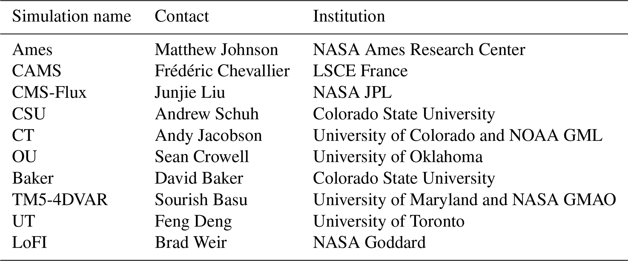
(Chen et al., 2012)Takahashi et al. (2009)(Weir et al., 2021)Table 1Configuration of each simulation used in the MIP comparison.

* This simulation has been used in the v9 MIP. LoFI uses a different method than the other inversions but fits some independent data as the other simulations do. In addition, it has the highest resolution. LoFI has then been used in this MIP project to look at a range of different methods, but, in this study, we will focus our analysis on the range of emissions from the other simulations.
The paper is structured as follows. The MIP design as well as data used in the inversions (i.e., the in situ data and OCO-2 v9 retrievals, as well as how v9 differs from v7) will be detailed in Sect. 2. In this same section the independent data used for evaluation will also be presented. Section 3 presents the optimized fluxes estimated from the in situ, v7 and v9 inversions at global, latitudinal, and regional scales. Evaluation using independent data will appear at the end of this Sect. 3. Finally, Sect. 4 will discuss the results and findings.
2.1 MIP design
The MIP project, organized by the OCO-2 Science Team, is a collaboration of CO2 modelers formed to study the impact of assimilating OCO-2 retrieval data into atmospheric inversion models. The project's goal is to create an ensemble of CO2 surface flux estimates to understand how flux estimates using OCO-2 retrievals and in situ measurements depend on (i) transport, (ii) data assimilation methodology, (iii) prior flux and associated errors, and (iv) possible systematic errors in the OCO-2 retrievals, in particular across viewing modes, i.e., ocean glint (OG), land nadir (LN), and land glint (LG). The OCO-2 MIP philosophically mimics past projects such as RECCAP (REgional Carbon Cycle Assessment and Processes) and TRANSCOM (The Atmospheric Tracer Transport Model Intercomparison Project) designed to analyze the uncertainty in inverse calculations of the global carbon budget resulting from errors in simulated atmospheric transport. MIP models are more strictly controlled or have more common elements than previous CO2 inverse model intercomparisons such as Peylin et al. (2013). Table 1 gives summary information of the different modeling systems and their transport models and configurations, while Table 2 gives the information of modelers' names and their respective institutions.
The LoFI (Low-order Flu Inversion) submission (Weir et al., 2021), new in the v9 MIP, is intended as an additional metric of flux inversion skill. LoFI uses in situ observations to match only the global atmospheric growth rate with an empirically derived land sink (Chevallier et al., 2009). The inferred fluxes are thus independent of the spatial and sub-annual variability in atmospheric observations and rely minimally, if at all, on model atmospheric transport representation. Despite the weak data constraint, LoFI is included below with the IS inversions because it depends on the annual, global growth rate determined from observations. Given the problems flux inversions have facing remote-sensing retrieval biases (O'Dell et al., 2018) and atmospheric transport errors (Schuh et al., 2019), LoFI serves as a first-order check on inversion skill. Times and places where a flux inversion outperforms or equals LoFI's skill suggest a nominally operating system, while significantly degraded skill suggests a problem, e.g., in the prior, atmospheric transport, and/or ingested data.
The modelers used NASA's operational bias-corrected OCO-2 L2 Lite XCO2 product v9 (Kiel et al., 2019, https://daac.gsfc.nasa.gov, last access: August 2019) in the v9 version of the MIP. The OCO-2 v9 dataset has an improved bias correction approach that results in reduced biases, particularly over areas of rough topography. While variations amongst inversion systems are considered beneficial for the purpose of characterizing flux uncertainty, some configurations needed to be standardized in order to avoid meaninglessly large differences in the ensemble spread. All inversion modelers were instructed to assimilate OCO-2 data from 6 September 2014 through 31 May 2019 and to submit estimated fluxes from 1 January 2015 through 31 December 2018 (to allow the flux estimate some time to spin up and down on either end). Fossil fuel emissions, which are typically not optimized in global top down studies (Peylin et al., 2013), were standardized for the project. Similar to the experiments described in Crowell et al. (2019), all modelers assumed the same monthly fossil fuel emissions from the Open-source Data Inventory for Anthropogenic CO2 (ODIAC2019; Oda and Maksyutov, 2011; Oda et al., 2018), modified with the TIMES diurnal and day-of-week scaling (Nassar et al., 2013).
Though fossil fuel emissions are fixed, all other prior flux estimates were chosen independently by each modeling group. For instance, regarding fire emissions, most models used the Global Fire Emission Database – either version 3 (GFED3) or version 4 (GFED4). GFED3 and GFED4 mainly differ on burned area, where small fires are included in version 4 (Randerson et al., 2012; Giglio et al., 2013). The added information of small-fire burned area increases the burned area particularly over agricultural and peat land regions (van der Werf et al., 2017).
2.2 OCO-2 retrievals
The NASA satellite OCO-2 was launched in July 2014 (Crisp et al., 2017; Eldering et al., 2017) and flies in a near-polar, sun-synchronous orbit (so ground tracks are spaced more closely at high latitudes than midlatitudes) at a 705 km altitude with a local crossing time at the Equator between 13:21 and 13:30 local time. OCO-2 flies in the Earth Observing System's (EOS) Afternoon Constellation (A-Train) and has a 16 d ground track repeat cycle that gives global XCO2 coverage twice per month with approximately 150 km longitudinal offsets between nearby revisiting orbits. OCO-2 has a spectrometer measuring sunlight reflected by the Earth and its atmosphere in three spectral bands: the oxygen A-band in the near-infrared (NIR) at 0.76 µm wavelength and two CO2 spectral bands in the shortwave infrared (SWIR) at 1.6 and 2.1 µm. OCO-2 provides spatially dense data with a narrow swath (no wider than 10 km) and with spatial footprints of a few square kilometers (less than 1.25 km by 2.2 km projected onto the surface). O'Dell et al. (2018) reported that the fine resolution of OCO-2 increased the number of cloud-free scenes. As is known, clouds are difficult to model, so having more cloud-free scenes yields more successful retrievals with lower errors.
The OCO-2 sensor provides observations in three modes. Nadir retrievals are those in which the satellite is looking at the Earth directly below, i.e., at the sub-satellite point. These retrievals are only usable when the instrument is directly over land. Glint retrievals are from measurements occurring when the instrument is pointed (usually off-nadir) toward the solar glint spot. Glint is the primary mode for over-ocean retrievals, as the ocean surface is very dark in the SWIR spectral range, only reflecting sufficient solar radiation near the glint point. Target mode retrievals are obtained when the sensor points at a fixed location along the orbit to keep a particular point on the Earth's surface in view and is employed mainly to collect validation data over locations such as TCCON sites. In this study, besides using land nadir and land glint separately from the v7 MIP, both land nadir and land glint mode retrievals combined together have also been used, providing data over the oceans. The advantage of combining both modes is to yield a stronger constraint at regional scales on CO2 fluxes (Miller and Michalak, 2020). In addition, biases existing between these two modes of retrievals have been reduced (O'Dell et al., 2018). In this study, we focused on the nadir and glint modes, so the target mode is not discussed further. In addition, we only focus on the land nadir (LN) and land glint (LG) modes and do not use the ocean observation mode. Even if, since version 7, ocean biases in OCO-2 retrievals have been largely reduced (O'Dell et al., 2018), inversions assimilating OCO-2 ocean retrievals produced unrealistic results with annual global ocean sinks higher of 2.6±0.5 Gt C yr−1 compared to the state-of-the-art estimated in Le Quéré et al. (2018), which was 2.5±0.5 Gt C yr−1 in 2017. Consequently, as for MIP v7 (Crowell et al., 2019), the OCO-2 ocean retrievals will not be further discussed in this study.
The algorithm developed to retrieve the column average dry-air mole fraction of CO2 in the atmosphere (XCO2) from the measured radiance spectrum comes from NASA's Atmospheric CO2 Observations from Space (ACOS) project (O'Dell et al., 2012; Connor et al., 2008). The ACOS algorithm was first applied to GOSAT NIR and SWIR spectral measurements, which have similar spectral characteristics to the OCO-2 measurements, before being used for OCO-2 and OCO-3 (which were launched at later dates). In addition to the spectral data, ACOS uses meteorology and model data to constrain retrievals of XCO2 along with a variety of other parameters such as aerosol optical depth, surface albedo, surface pressure, and total-column water vapor. In this paper, the modelers have used the ACOS bias-corrected retrievals (OCO-2 Level 2 Lite XCO2 product) version 9 (Kiel et al., 2019; O'Dell et al., 2018, https://daac.gsfc.nasa.gov, last access: August 2019). Since October 2019, OCO-2 processing has used the ACOS version 9 (or “ACOS B9”) algorithm, an update to the previous v7 and v8 versions (O'Dell et al., 2018). Several changes have been applied in the v9 compared to the v7. In particular, the v8 data included corrections related to the spectroscopy, aerosol treatment, prior meteorology, and the surface model. More details can be found at O'Dell et al. (2018). v9 included an addition correction for the surface pressure estimation (Kiel et al., 2019) which significantly reduced biases, particularly over areas of rough topography. This bias correction in v9 allows a more uniform distribution of XCO2 over regions of interest, decreasing the standard deviation over the TCCON Lauder (New Zealand) site, for instance, to 0.74 ppm compared to v8, which was 1.35 ppm.
MIP modelers used all valid cloud-free OCO-2 retrievals (those regarded as “good” by the quality_flag xco2_quality_flag=0) from the OCO-2 Lite files and then selected the bias-corrected data (Wunch et al., 2011). Since the spatial resolution of OCO-2 data is much higher than the model grid box scale used in the inversions, the OCO-2 data are averaged to a coarser scale (in this study, across a 10 s span, equivalent to about 67.5 km, along track) before being assimilated. The retrieved column CO2, averaging kernels, prior CO2 profiles, and a subset of the auxiliary parameters from the Lite files have all been averaged across these 10 s spans in the same way, weighted by the inverse of the square of the retrieval uncertainty (variable xco2_uncertainty) for each scene in the average. This is similar to the averaging done for the OCO-2 v7 MIP (Crowell et al., 2019), except that the 10 s averages are calculated directly, without the intermediate step of computing 1 s averages, as was done before. In computing the uncertainty to be placed upon the new 10 s average XCO2 value, an attempt was made to account for correlations between the model–data mismatch (MDM) errors for each individual scene: each scene within the 10 s span was assumed to have errors that were correlated with every other scene in the span with the same positive correlation coefficient (+0.3 and +0.6 for scenes over land and ocean, respectively). Details of the form and derivation of these average uncertainties may be found in the “constant correlation” section of Baker et al. (2021). The approach to handling the correlations, while crude, represents an increase in complexity compared to what was assumed in the v7 MIP (no reduction in uncertainty due to the averaging process, as described in Crowell et al., 2019). Since it is known that the uncertainty computed by the retrieval (in variable xco2_uncertainty) underestimates the true level of error in the retrieved XCO2, an additional term is added onto this “theoretical” uncertainty, in quadrature, to obtain a more realistic uncertainty per scene: σSD, the standard deviation of all the XCO2 values used in the 10 s average. In this ad hoc approach, scenes that have a very small spread in XCO2 values across the 10 s span are assigned the theoretical uncertainty from the retrieval, while those for which the actual variability of the XCO2 values is larger than the theoretical values are assigned a value closer to this computed error level. Both of these uncertainties are then passed through Eq. (39) from Baker et al. (2021) to account for error correlations. Finally, an additional error term, σtransport, is added in quadrature to account for transport model errors. With all three of these terms considered, the square of the uncertainty in the 10 s XCO2 average is given as
where
and where and σj are the individual XCO2 values going into the average and their retrieval uncertainties, and N is the number of good 10 s XCO2 values in the 10 s average. The transport model error term is computed from the difference between the CO2 concentrations computed by the TM5 and GEOS-Chem models when both are driven by the same realistic surface CO2 fluxes, after the annual mean difference field is subtracted; the values that result are considerably smaller than those model errors added for the OCO-2 v7 MIP (Crowell et al., 2019). In contrast to this level of detail, the errors between different 10 s averages are assumed to be independent when assimilated into the inversions (Worden et al., 2017; Crowell et al., 2019). Several studies have used this assumption, deeming it appropriate for the resolution of their inversions or simulations (Basu et al., 2018; Chevallier et al., 2019).
2.3 In situ CO2 measurements
The set of in situ CO2 measurements used for assimilation and for evaluation is drawn from five collections in ObsPack (Masarie et al., 2014, and https://www.esrl.noaa.gov/gmd/ccgg/obspack/, last access: August 2019) format. These component ObsPacks are
-
obspack_co2_1_GLOBALVIEWplus_v5.0_2019-08-12 (Cooperative Global Atmospheric Data Integration Project, 2019). This is the main source of in situ CO2 measurements for MIP experiments, contributing 93 % of all in situ measurements. It extends through the end of 2018.
-
obspack_co2_1_NRT_v5.0_2019-08-13 (NOAA Carbon Cycle Group ObsPack Team, 2019). This near real-time ObsPack distribution is intended to provide data records after the end of the GLOBALVIEW+ v5.0 product, for laboratories and datasets that can provide measurement data outside of an annual update cycle. These data are provisional and generally have not undergone final quality control.
-
obspack_co2_1_AirCore_v2.0_2018-11-13. The balloon-borne AirCore instrument samples almost the entire atmospheric column. This early release collected all available profiles between 2014 and 2018.
-
obspack_co2_1_INPE_RESTRICTED_v2.0_2018-11-13 (NOAA Carbon Cycle Group ObsPack Team, 2018). This provides aircraft profiles at five sites in Brazil.
-
obspack_co2_1_NIES_Shipboard_v2.1_2019-06-12. This provides continuous CO2 analyzer measurements from nine volunteer ships of opportunity operated by the Japanese National Institute for Environmental Studies (Tohjima et al., 2005; Nara et al., 2017).
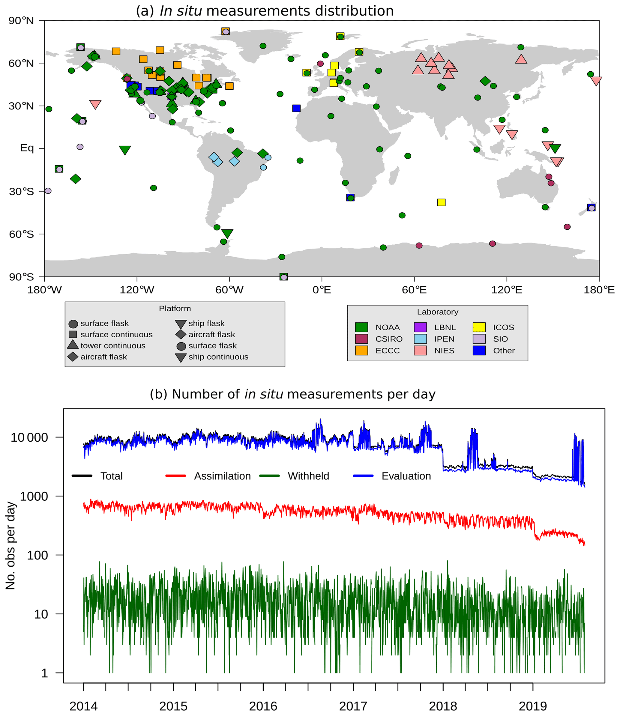
Figure 1(a) Distribution of assimilated in situ measurements around the world. The instrument platform is indicated by marker shape, whereas the color represents the laboratory collecting the data. NOAA is the United States National Oceanic and Atmospheric Administration, CSIRO is the Australian Commonwealth Scientific and Industrial Research Organisation, ECCC is Environment and Climate Change Canada, LBNL is the Lawrence Berkeley National Laboratory, IPEN is the Brazilian Instituto de Pesquisas Energeticas e Nucleares, NIES is the Japanese National Institute for Environmental Studies, ICOS is the European Union Integrated Carbon Observation System, and SIO is the Scripps Institute of Oceanography. Mobile shipboard programs are shown with a single marker at the mean location of the measurements. Figure from Jacobson et al. (2020a). (b) Number of in situ measurements available per day, broken down by usage category. The total number of measurements (black) is the sum of assimilated (red), withheld (green), and evaluation (blue) data. The reduction in evaluation data at the end of 2018 corresponds to the end of available measurements from the Comprehensive Observation Network for Trace gases by Airliner (CONTRAIL) projects. The reduction in assimilated measurements at the end of 2019 corresponds to the transition from GLOBALVIEW+ to near real-time (NRT) data. Intermittent spikes in evaluation data are linked to campaigns like ATom and ACT-America.
This collection runs from 1 January 2000 to 31 July 2019 with an average of about 520 assimilable observations and 17 withheld observations per day (see Fig. 1b). Measurements are contributed by 56 laboratories around the world. Measurements are collected at surface flask sites, at observatories and towers with continuous analyzers, onboard research and commercial ships, from light aircraft at regular profiling sites, from balloon-borne AirCore samples, and on commercial aircraft (see Fig. 1a)
Only a small subset of ObsPack measurements are designated as suitable for assimilation, and the remainder are designated for evaluation. The assimilable measurements meet two criteria: they can be successfully simulated in coarse-resolution global models, and they can be assigned an MDM error value. Many factors can render observations difficult to simulate in the global models used for this exercise. Sites located in areas with complex topography or close to strong local sources like cities or strongly influenced by small-scale circulation features such as land–sea breezes are all considered difficult to simulate. The CarbonTracker “adaptive model–data mismatch” scheme from CT2017 (Peters et al., 2007, with updates documented at http://carbontracker.noaa.gov, last access: August 2019) was used to assign MDMs for this experiment. The MDM represents the expected statistical model residual from a measured value, and the current scheme estimates MDM values that vary by geographic location, month of year, local solar time of day, and distance from the Earth surface. These values are developed using model performance from previous simulations, by computing a climatology of expected model errors for a given dataset. These model errors are driven both by faults in simulated atmospheric transport and by incorrect upstream fluxes, but it is only the first of these that we attempt to represent with MDM. At many sites, model performance is dominated by a conspicuous cycle of seasonal error, attributed mostly to high ambient variability of CO2 in the local growing season. Exploratory analysis has demonstrated that model-to-model differences in performance are significantly smaller than the other sources of variability in MDM like this annual cycle of model error.
The adaptive MDM scheme requires sufficient repeated measurements to develop a climatology of model performance, and as a result does not provide estimates of MDM error for measurements from temporary field deployments and aircraft campaigns (e.g., ACT-America – DiGangi et al., 2018 – and ATom – Wofsy and ATom Science Team, 2018). Many of these measurements without an MDM value are otherwise assimilable, since they sample background conditions that models should be able to simulate successfully. These data are particularly useful for model evaluation because they are generally independent of assimilated measurements.
2.4 Withheld data
In order to evaluate inversion model performance, a small subset of the assimilable in situ measurements were withheld for cross-validation. Each withheld measurement has an MDM value, which allows model residuals to be normalized by expected performance. The collection of withheld measurements was then used to evaluate the MIP ensemble.
Approximately 5 % of the assimilable data was chosen for withholding. These were chosen carefully to maximize independence from the data designated for assimilation in the IS experiment. The criteria for withholding vary by measurement type. Flasks, which are generally taken on a weekly basis and with sampling criteria that emphasize background conditions, are already assumed to be independent from one another. All the measurements in a given aircraft profile are assumed to be related, so entire profiles were excluded. Quasi-continuous measurements, like those at towers and observatories, are assumed to be correlated in time, so all measurements during 5 % of entire days were excluded.
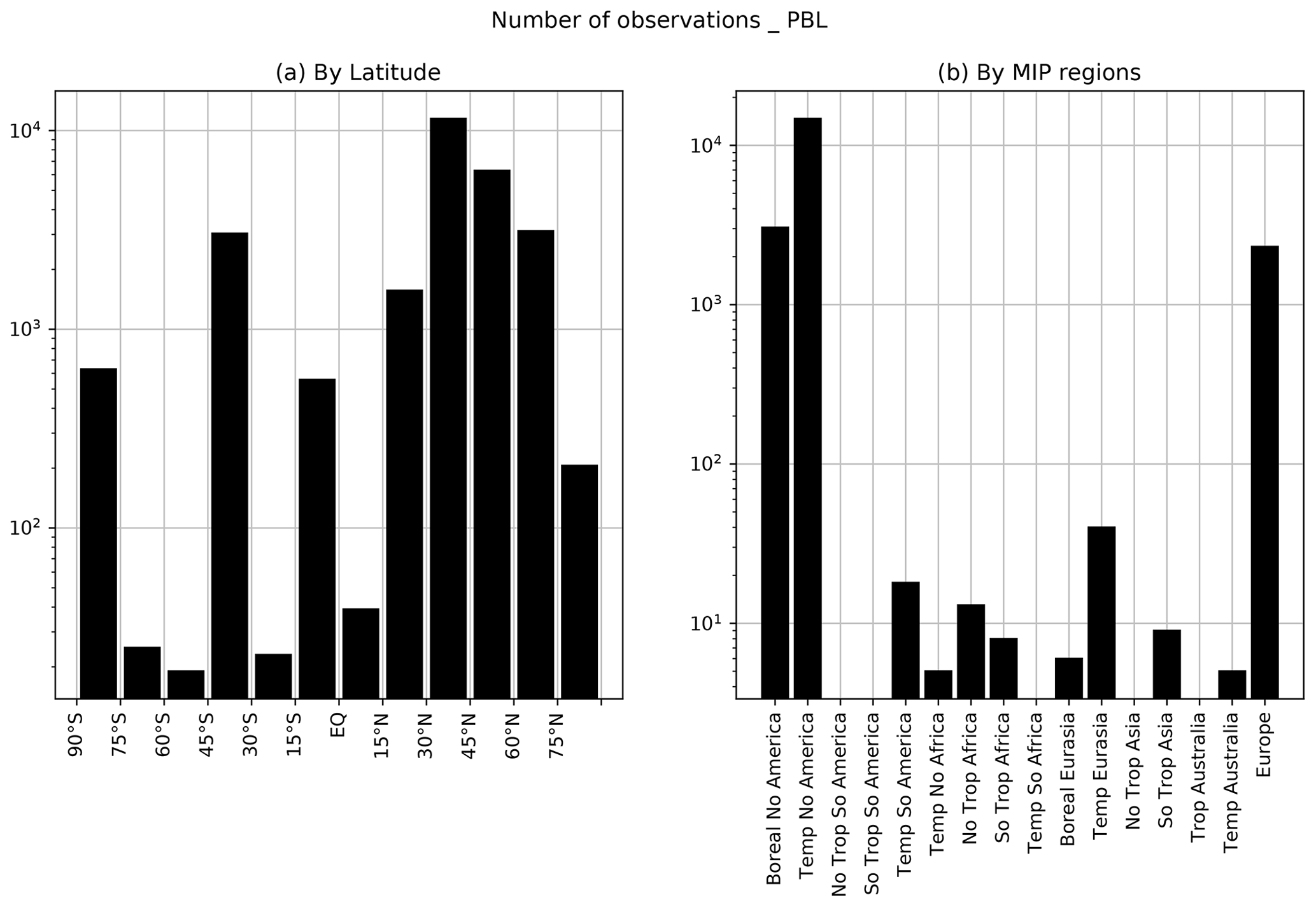
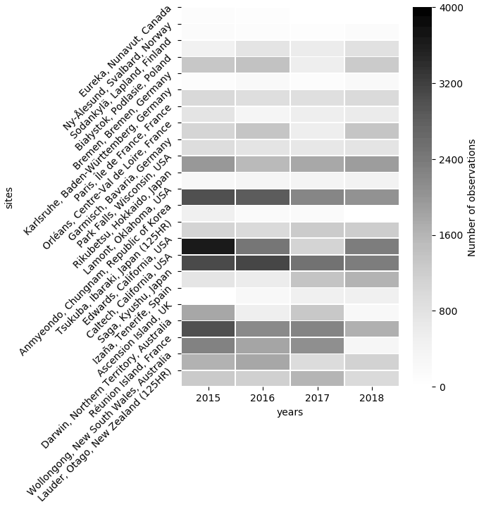
Figure 2Number of withheld observations by latitude (a) and by MIP region (b) in the planetary boundary layer (PBL).
Figure 2 shows the number of withheld data available for evaluation by latitude (Fig. 2a) and by MIP region (Fig. 2b). There are only about 1000 data points in the Southern Hemisphere and approximately 600 in the tropics, in contrast to 5300 in the Northern Hemisphere. For example, Fig. 2b shows the dearth of withheld observations for tropical regions such as north and south Africa. There are no withheld data at all for some MIP regions, such as northern tropical Asia and tropical South America.
2.5 ATom measurements
Atmospheric concentrations of CO2 collected during the airborne campaigns of NASA's Atmospheric Tomography (ATom) mission (Stephens, 2017; Wofsy and ATom Science Team, 2018) are particularly useful for evaluation. These measurements come from four campaigns conducted over the Pacific and Atlantic oceans between 2016 and 2018. The ATom samples have been binned into five altitude levels (approximately of 0–1, 1–3, 3–7, 7–10, and 10–14 km) and nine latitude bins (every 15∘ latitude) for evaluation (Sect. 3.4). The density of ATom measurements by latitude and altitude bin are shown in Fig. 16, which will be discussed in Sect. 3.4.
2.6 TCCON
The Total Carbon Column Observing Network (TCCON) is composed of around 30 sites around the globe estimating column-averaged dry-air mole fraction of several atmospheric gases using ground-based remote sensing by Fourier transform spectrometers (Wunch et al., 2011). TCCON measures spectra of direct sunlight in the near-infrared region. TCCON CO2 retrievals are estimated to have precisions better than 0.25 % (1σ) (Wunch et al., 2011). These retrievals have been used as the primary validation resource for several satellite missions, including OCO-2, SCIAMACHY, and GOSAT (Wunch et al., 2011, 2017). OCO-2 observations were extensively evaluated against TCCON data in Wunch et al. (2017).
Posterior and prior concentrations are sampled for each 30 min average TCCON retrieval before calculating the statistics following the approach described in Crowell et al. (2019). For LNLGv9 inversions, the available 10 s prior and posterior XCO2 simulated retrievals were averaged and compared to TCCON observations with a 5∘ latitude and longitude geometric coincidence criterion and within 1 h of the overpass. All TCCON sites used in the evaluation section are listed in Table 3, and Fig. 3 represents the location of the TCCON sites. Figure 4 illustrates the different time ranges and observation numbers across TCCON sites during the 2015–2018 period.
Strong et al. (2019)Notholt et al. (2014)Kivi et al. (2014)Deutscher et al. (2019)Notholt et al. (2014a)Hase et al. (2015)Té et al. (2014)Warneke et al. (2019)Sussmann and Rettinger (2018)Wennberg et al. (2017)Morino et al. (2018b)Wennberg et al. (2016)Goo et al. (2014)Morino et al. (2018a)Iraci et al. (2016)Wennberg et al. (2014)Kawakami et al. (2014)Blumenstock et al. (2017)Feist et al. (2014)Griffith et al. (2014a)De Mazière et al. (2017)Griffith et al. (2014b)Sherlock et al. (2014)Table 3Geolocation and reference of each TCCON station used for the evaluation section.

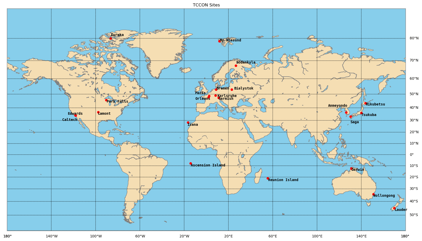
Figure 3Locations of the TCCON sites used in this study over the globe.
We discuss results from two v9 MIP experiments: IS, in which only the in situ CO2 measurements are assimilated, and LNLGv9, for which OCO-2 v9 land nadir and land glint retrievals were assimilated together. The v9 MIP simulations are conducted over the 4 years from 2015–2018. For comparison, we also include results from the v7 MIP LNv7 and LGv7 experiments (Crowell et al., 2019), although those results are limited to 2015 and 2016 only. In both the v7 and v9 MIPs, ocean glint retrievals were also assimilated in separate experiments. Those experiments will not be discussed here, as the ocean glint retrievals have uncharacterized biases in both v7 and v9 versions. For the purpose of analysis, the standardized fossil fuel emissions have also been removed from all prior and posterior fluxes. Figure A1 in the Appendix represents the location of the OCO-2 10 s retrievals LNLGv9 for the period of study 2015–2018. We can see that the posterior flux estimates are constrained with OCO-2 LNLG observations particularly present in the Northern Hemisphere and with a lower number of observations over the tropics.
This section is organized as follows: we first analyze fluxes at the global scale before moving to three broad zonal bands. We then finish with a regional flux analysis. In order to evaluate the spatiotemporal variability of regional fluxes, the different modeling groups' flux estimates have been aggregated from their individual model grid boxes up to OCO-2 MIP regions (see Fig. 5) similar to those used in the MIP v7 analysis from Crowell et al. (2019).
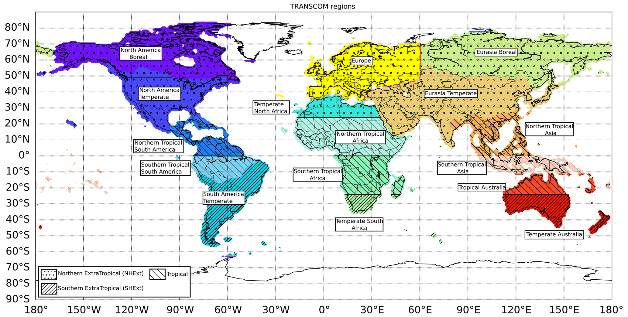
Figure 5OCO-2 MIP regions to which gridded fluxes are aggregated for comparison and evaluation.
3.1 Global flux estimates
Figure 6 represents the median annual emissions (in Pg C yr−1, for Fig. 6a, c, and e) and the monthly median emissions (in Pg C month−1 for Fig. 6b, d, and f) at the global scale for each experiment. As expected, at the global scale the posterior fluxes of all OCO-2 observation types, as well as the prior and IS emissions, have a similar seasonal cycle (Fig. 6b). Fluxes for all of the models are well constrained at this scale as they are the difference of the relatively well-known fossil fuel fluxes and the well-measured global atmospheric increase. However, the peak sinks during the Northern Hemisphere growing season (from May through September) are slightly larger with OCO-2 v7 than with OCO-2 v9. The large sink observed at a global scale during this season is due to the strong biospheric uptake of CO2 in the temperate and boreal forest of the Northern Hemisphere (Friedlingstein et al., 2020). Additionally, while the growing season observed with v7 is shifted earlier in the year relative to IS and the unoptimized prior fluxes, this is not the case with v9 (although the priors in the v7 and v9 MIPs are not the same for some models, this could also be due to the longer number of years in the v9 experiments and the models participating in the two MIP versions). While the median values for the prior emissions of the land plus ocean fluxes in v7 were around −2.5 Pg C yr−1 in 2015–2016 (Fig. 3a in Crowell et al., 2019), they are around −3.75 Pg C yr−1 for the same period (2015–2016) in v9 (Fig. 6a) and have a smaller ensemble spread among the models.
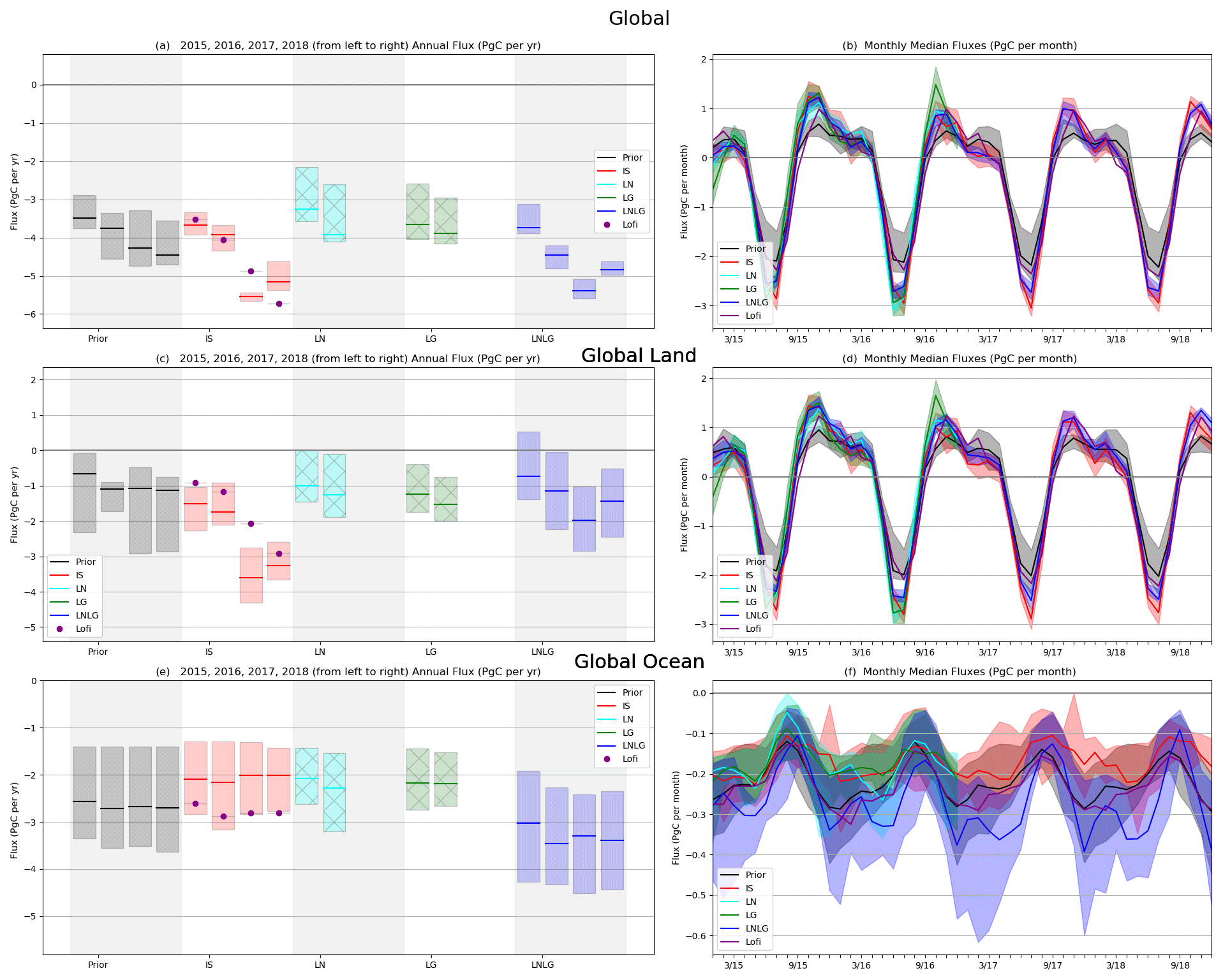
Figure 6Monthly median fluxes in Pg C month−1 (b, d, f) and annual flux in Pg C yr−1 (a, c, e) from 2015 through 2018 for the different experiments: prior (black) and posterior ensemble fluxes constrained by in situ data (red), OCO-2 v7 LN (cyan with hatched cross), OCO-2 v7 LG (green with hatched), and OCO-2 v9 LNLG (blue) retrievals. LoFI fluxes (purple circles) are plotted alongside IS fluxes. For both the monthly time series and the annual fluxes plots, the shaded bar represents the range of emissions among the models and the solid lines represent the median of the model ensemble for both annual and monthly plots. Top plots are for global (land + ocean), middle plots for global land and bottom plots for global ocean.
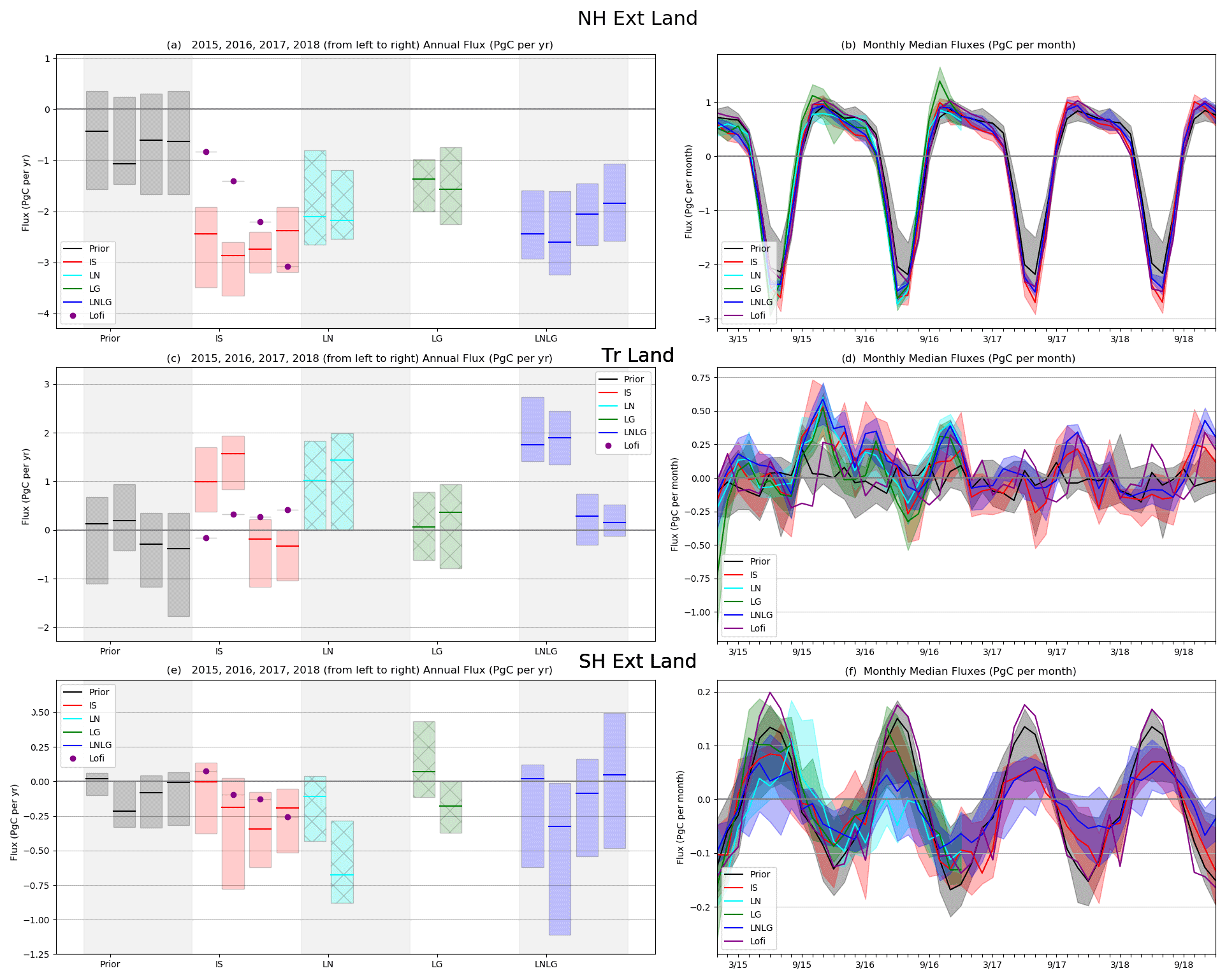
Figure 7Same as Fig. 6 but for the zonal band: northern extra-tropics (NHExt, a, b) with latitudes from 23–90∘ N, tropics (c, d) with latitude from 23∘ S–23∘ N, and southern extra-tropics (SHExt; e, f) with latitude from 90–23∘ S.
For the annual total fluxes, at the global scale, we can observe a good agreement between IS and all OCO-2 fluxes in 2015 with emissions of approximately −3.75 Pg C yr−1. However, in 2016, LNLGv9 gives a stronger sink of Pg C yr−1 compared to IS and v7 with a sink median around −4 Pg C yr−1. This stronger sink observed with v9 in 2016 comes from southern extra-tropics (Fig. 7e). For 2017 and 2018, both IS and v9 are very close to each other with total annual sinks between and Pg C yr−1. The ensemble spread among the models for the annual fluxes is smaller with v9 than with v7, which could either be due to the longer span of data inverted in v9 where the ability to compute the trend (or the total land + ocean flux) improves, reducing noise in the estimates, or it could suggest better agreement between the models for the v9 version. With a 4-year record of flux estimates from both IS and LNLGv9, we are able to group 2015 and 2016 together. These are years which have been associated with a large CO2 growth rate due to a strong El Niño event (Malhi et al., 2018) compared to 2017 and 2018. For the rest of this study, we will call the 2015–2016 period the “El Niño period” and the 2017–2018 period the “recovery period”. Several previous papers have already studied these periods, focusing on the impact of El Niño over the tropics (Liu et al., 2017; Palmer et al., 2019; Wigneron et al., 2020). The contrast between these two different periods can also be observed over the global land in particular, where the difference between the El Niño period and recovery is particularly large in the IS inversions. Global land (Fig. 6c and d) and global ocean (Fig. 6e and f) show a compensating effect, where v9 finds higher sources during the El Niño period over the land that are balanced with stronger sinks over the ocean. Generally v9 yields a weaker global land sink and stronger ocean sink. During the recovery period, IS gives a stronger median sink (3.5 Pg C yr−1) than v9 (1.75 Pg C yr−1). Friedlingstein et al. (2020) estimated a global land uptake of around 2 Pg C yr−1 in 2018 over the global land for the net fire and biospheric fluxes, which is closer to what we see constrained by the v9 data.
3.2 Latitudinal bands
As mentioned in Crowell et al. (2019), the observations should constrain the fluxes over latitudinal bands more effectively than longitudinally or by geopolitical region, due mainly to the effects of prevailing zonal winds across much of the globe. OCO-2 observations are collected across the sunlit portion of the Earth crossing all zonal bands about 15 times per day. Hence we split our analysis between the tropics and extra-tropics, examining only land emissions since we expect the data constraint to be strongest there for the mostly land-based observations that we discuss. Over the northern extra-tropics (Fig. 7b), we observe flux dynamics similar to those on the global scale, with large seasonal variation and deeper sinks during summer for OCO-2 and IS inversions compared to the prior. All experiments put the land sink more in the northern extra-tropics than in the tropics and southern extra-tropics (Tans et al., 1990).
For the annual fluxes (Fig. 7a), we can see that IS and LNLGv9 northern extra-tropics fluxes are close to each other in 2015–2016, with an increase in net carbon uptake relative to the prior of around 2.5±0.25 to 3±0.25 Pg C yr−1 in 2015 and 2016, respectively. In 2017 and 2018, we can observe a decrease in net carbon uptake larger with v9 (fluxes of around 2 Pg C yr−1 in 2017 and 1.75±0.25 Pg C yr−1 in 2018) than IS (2.75 Pg C yr−1 in 2017 and 2.5±0.25 Pg C yr−1 in 2018).
We also see some differences between v7 and v9. LNv7 fluxes are closer to what is observed in both LNLGv9 and IS during the El Niño period, with a median sink around −2.25 Pg C yr−1, but LGv7 gives a weaker sink (−1.5 Pg C yr−1) due to larger sources in fall 2015 and 2016. As we can observe for all other latitudes bands and we will observe for smaller regions, LNLGv9 tends to be closer to LNv7 than to LGv7. This points to previously known issues with the v7 LG data that were resolved with a unified bias correction in OCO-2 v9. Interestingly, the seasonality for the v9 results more closely aligns with the IS results, and the large efflux at the end of the growing season in v7 LNLG has disappeared in v9.
The southern extra-tropics (SHExt, Fig. 7e and f) are known to have fewer IS observations as well as little land mass (Crowell et al., 2019) and hence fewer land retrievals to constrain the fluxes, which are significantly weaker over this latitude band. This could explain why, for this latitude, the prior, IS, v7, and v9 results have different seasonality. LNv7 and LNLGv9 have different seasonality and v7 has a delay in the efflux peak for 2015 and no efflux peak at all for 2016. The seasonal amplitude observed with LNLGv9 is smaller for the whole period compared to IS and LGv7 and has a delay in 2017 and 2018 compared to IS. The lack of IS data over this latitudinal band could explain the differences in seasonality and sink values between IS and LNLG. The differences in monthly emissions are also observed in the annual fluxes. They show, for the whole period, stronger sinks with v9 than with IS and v7. However, in contrast to the northern extra-tropics (NHExt), the ensemble spread is larger with v9 than with v7. The bias reduction of v9 gives a smaller spread and hence a better agreement among the models, particularly over the Northern Hemisphere.
Over the tropics (Fig. 7c and d), the seasonal peak efflux is typically in the fall, with an anomalously strong source in fall 2015 during the El Niño intense period. On average, the seasonality seems to be similar for the IS and OCO-2 inversions but different from that of the prior. However, for the whole period, the v9 OCO-2 annual mean source is about 0.5±0.1 Pg C yr−1 stronger than for IS. OCO-2 observations have a more frequent coverage over the tropics than the in situ network. However, OCO-2 retrievals can be biased due to cloud coverage during the wet season and aerosol from biomass burning during the dry season (Merrelli et al., 2015; Massie et al., 2017). LNLGv9 gives stronger annual sources, particularly for the El Niño period, and with a smaller ensemble spread than does v7. The OCO-2 LGv7 ensemble spread does not deviate from the prior spread, showing the large impact of v9 corrections on the retrievals. We can also observe that the IS ensemble spread does not deviate from the prior spread. Neither IS nor LNLGv9, for each model, follows their priors in the tropics during the period of study (not shown here). The in situ Obspack dataset used for this study has been updated and includes more data per site, contrary to the in situ dataset used in Crowell et al. (2019) for the v7 MIP. We then have stronger sources observed with ISv9 than with ISv7 in 2015 and 2016. In addition, we can observe with both IS and LNLGv9 two clearly distinguished periods in terms of annual mean flux: the El Niño period for 2015 and 2016, with sources between 1.5 and 2 Pg C yr−1, and the recovery period, with median values between −0.5 and 0.5 Pg C yr−1. For both monthly and annual fluxes, large sources of carbon are observed over the tropics for the whole period of study. Wigneron et al. (2020) found that the pan-tropical above-ground carbon stocks in the tropical humid forests did not recover after the 2015–2016 El Niño, due presumably to a combination of deforestation and climate conditions.
3.3 Fluxes by region
3.3.1 Northern extra-tropical region
We see similarities in the seasonality and annual flux across zonal bands in the OCO-2 (mainly v9) and IS results for the northern extra-tropics but also differences between v7 and v9: now we look at smaller spatial scales to see where these agreements or disagreement are observed. Figure 8 shows monthly and annual fluxes for North America (Fig. 8a and b), Europe (Fig. 8c and d), and northern Asia (Fig. 8e and f).

Figure 8Same as Fig. 6 but for the northern extra-tropics regions: North America (a, b), Europe (c, d), and northern Asia (e, f).
Over North America (Fig. 8a and b), monthly and annual fluxes show different patterns for all data types. Prior annual median fluxes are around −0.25 Pg C yr−1 for 2015–2018. Median values for LNLGv9 show 0.5 Pg C yr−1 stronger sinks during the El Niño period, with LNv7 showing even deeper sinks. IS and LGv7 have deeper sinks than the prior but weaker than LNv7 and v9.
Over Europe, we can see that IS agrees better with LNLGv9, with similar annual median fluxes. For this region, v7 and v9 are particularly different, as v9 gives larger sinks during summertime. Interestingly, LNLGv9 seems then to be in a better agreement with what was observed in Houweling et al. (2015) than v7. Houweling et al. (2015) assimilated GOSAT data over the 2009 and 2010 period and observed a larger carbon uptake for Europe with GOSAT than with in situ data, as was also observed by Chevallier et al. (2014) and Reuter et al. (2014). Inferred fluxes using v9 seem then to be more consistent with other studies, but more analysis is needed to understand why this difference between v7 and v9 appears over Europe (which could be due to a dipole between Europe and northern Africa as observed and mentioned by the previous studies of Houweling et al., 2015; Chevallier et al., 2014; Feng et al., 2016; Reuter et al., 2014, and Reuter et al., 2017) but not for North America and northern Asia. Previous studies already observed and mentioned a larger European land sink in balance with a large tropical land source. Specifically, Houweling et al. (2015) found a difference in flux between these two regions of around 0.8 Pg C yr−1. They found that this balance was caused by a lack of GOSAT observations during the winter over Europe. Additionally, Chevallier et al. (2014) also observed this balance between Europe and northern tropical Africa in their GOSAT inversions, and they considered the large source over North Africa as unrealistic. According to Feng et al. (2016)), the large sink over Europe, inferred from GOSAT data, was caused by large biases outside of the region; for mass balance, the inversions was removing more CO2 over Europe, in agreement with Reuter et al. (2014, 2017).
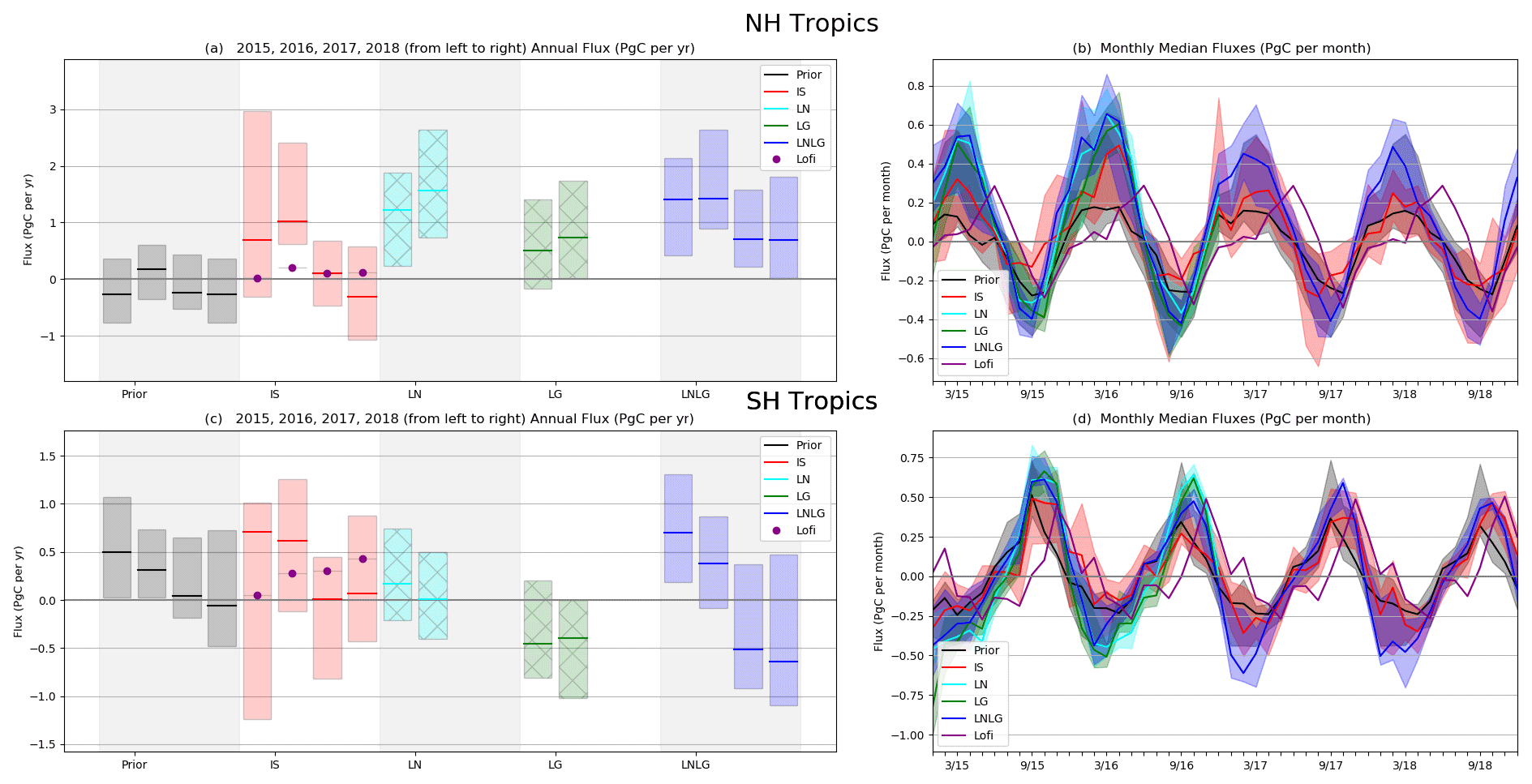
Figure 9Same as Fig. 6 but for the tropical band: northern tropics (a, b) with latitudes from 0–23∘ N and southern tropics (c, d) with latitude from 23–0∘ S.
For northern Asia (including temperate Eurasia and boreal Eurasia), while IS gives large sinks (with an ensemble spread between −2.5 and −0.5 Pg C yr−1 for the whole period), v9 and v7 both show weaker sinks (with an ensemble spread between −1.25 and −0.25 Pg C yr−1 for 2015 and 2016) and a decrease with v9 for 2017 ( Pg C yr−1) and 2018 ( Pg C yr−1). The 2017 and 2018 LNLGv9 emissions are closer to the priors. For the El Niño season (2015 and 2016), LNv7 has the same annual emissions as LNLGv9 but with a smaller ensemble spread; however, LGv7 shows weaker sinks with particularly strong emissions during the fall, which could be due to either fewer observations or a possible bias at higher latitudes during the Northern Hemisphere winter. The disagreement between the OCO-2 and in situ inversions might be driven by the differences in the amount of data assimilated since both inversions have the same transport model and inverse setup. We know that there are fewer in situ than OCO-2 observations above northern Asia, and particularly above the boreal forest of Eurasia, which is an important area for sources and sinks of atmospheric CO2 (Houghton et al., 2007; Siewert et al., 2015). The combination of sparse data, in an area not well observed, with transport uncertainty could be the cause. We see that the ensemble spread of the models is larger for IS than for v7 or v9 and that the annual fluxes differ by almost 1.5 Pg C yr−1 between the IS and OCO-2 inversions during the El Niño period. This is not the case for Europe and North America, where the surface measurements are most densely concentrated (Fig. 1a). Finally, due to the additional 2 years of fluxes using IS and v9, we see a trend towards a weaker sink from 2015 to 2018 for northern Asia that is not observed for Europe or North America. Further investigation is needed to explain the decrease in the carbon sink in this region with both IS and v9.
3.3.2 Tropical region
We now look at the tropics split across the Northern and Southern hemispheres. The southern and northern tropics are represented in Fig. 9, with annual fluxes on the left side (Fig. 9a and c) and monthly fluxes (Fig. 9b and d) on the right side of the plots. As observed earlier for the tropical band, and in contrast to what was found in Crowell et al. (2019) using the in situ data, the IS inversions give similar seasonal amplitude and annual mean emissions as OCO-2 for both the northern and southern tropics in 2015 and 2016, the El Niño period. However, for 2017 and 2018, IS seems to follow the pattern of the prior at the annual timescale. This difference, particularly for the northern tropics, in 2017–2018 seems to suggest a different signal observed with IS compared to v9. We can also observe that the ensemble spread is almost the same between both version v7 and v9 for both tropical bands. In both tropical hemispheres, LNv7 gives relatively more net CO2 emitted to the atmosphere than LGv7. LNLGv9 agrees with LNv7 over 2015–2016 for the northern tropics, but gives more of a source (0.5 Pg C yr−1) than LNv7 (0.1 Pg C yr−1) and LGv7 (−0.4 Pg C yr−1) over the southern tropics. This 0.5 Pg C yr−1 source of carbon observed with v9 is also observed with IS, suggesting that more carbon could have been released during the El Niño period than previously inferred with v7. During the recovery period in the northern tropics, v9 only has net sources of carbon, while for IS some models have sinks of up to −1 Pg C yr−1. In contrast, over the southern tropics, the median CO2 flux values given by IS are positive, while they are strongly negative for v9.
In order to see the resolution provided by the data at finer scales in the tropics, we examine fluxes for six tropical regions (three over the northern tropical hemisphere (Fig. 10) and three over the southern tropical hemisphere; Fig. 11).

Figure 10Same as Fig. 6 but for the northern tropical regions: northern tropical South (so) America (a, b), northern tropical Africa (c, d), and northern tropical Asia (e, f).
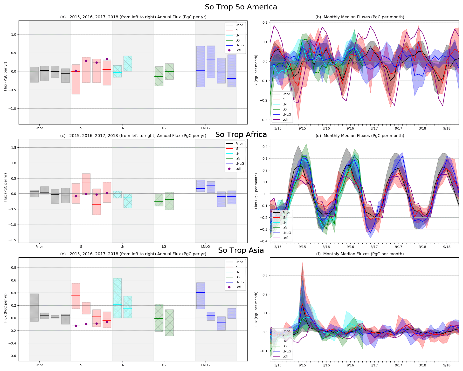
Figure 11Same as Fig. 6 but for the southern (So) tropical regions: southern tropical South America (a, b), southern tropical Africa (c, d), and southern tropical Asia (e, f).
Figure 10 shows the monthly and annual fluxes over northern tropical South America, northern tropical Africa, and northern tropical Asia. When we look at the annual fluxes of the northern tropical regions (Fig. 10a, c, and e), we do not observe significant differences between v7 and v9 inversions with respect to the ensemble spread and the median values, except for northern tropical South America, where v9 has a slightly higher net CO2 outgassing (0.5 Pg C yr−1) than v7 (around 0.4 Pg C yr−1 for LNv7 and 0.2 Pg C yr−1 for LGv7). The IS and OCO-2 annual fluxes have a similar temporal pattern over north tropical South America, with average fluxes close to 0.5 Pg C yr−1 and a smaller ensemble spread for OCO-2 than for IS. But the most obvious differences appear between the IS and OCO-2 inversions over northern tropical Africa and northern tropical Asia. The OCO-2 inversions give a larger source of carbon over northern tropical Africa compared to the IS inversions, similar to conclusions from the v7 MIP (Crowell et al., 2019). These large inferred emissions are consistent with Palmer et al. (2019) and Wigneron et al. (2020), who found that the Africa continent accounted for 56 % of carbon emissions during the 2015 El Niño event. However, for northern tropical Asia, both v7 and v9 give sinks of carbon (around −0.25 Pg C yr−1 for LNv7 and v9 and −0.4 Pg C yr−1 for LGv7), while IS gives a source of around 0.25 Pg C yr−1 during the El Niño season. Northern tropical Asia is the only region where we found a change in fluxes between the in situ inversions used in the v7 MIP and in the v9 MIP. Indeed, the v7 IS inversions (Crowell et al., 2019) had a median value for 2015 and 2016 of −0.10 Pg C yr−1 over northern tropical Asia. Sparse in situ coverage over the tropical regions compared to the Northern Hemisphere (Fig. 1a) could explain this difference with the OCO-2 inversions, but further analysis over this region needs to be done. The monthly seasonality is more similar between all experiments for northern tropical Africa than it is for the two other northern regions.
Looking at the monthly emissions of the southern tropical regions (Fig. 11), we can see the strong impact of El Niño between August and November 2015 over southern tropical Asia. The emissions reach a maximum of 0.35±0.01 Pg C yr−1, larger by around 0.30 Pg C yr−1 compared to the rest of the period. The large emissions from southern tropical Asia (Fig. 10f) primarily come from Indonesian fires. Field et al. (2016) estimated fire emissions in 2015 over Indonesia to be 380 Tg C. This El Niño impact started in the end of 2014, peaked in fall 2015, and ended in May 2016 (Liu et al., 2017). The impact of the El Niño is particularly noticeable with the long period available from v9 compared to the 2 years from v7. In addition, this peak is reflected in the annual mean fluxes, where v9 gives a strong separation between 2015 and the rest of the period (2016 and the recovery period), which is also observed with the IS. Annual median fluxes between v7 and v9 are almost similar, with sources in 2015–2016 of around 0.2 Pg C yr−1 (−0.05 Pg C yr−1) with LNv7 (LGv7) and of 0.4 Pg C yr−1 with v9. Similarly, even if there is a change in data coverage between the two versions, we do not observe much difference between v7 and v9 for southern tropical South America (Fig. 11a and b), except that the ensemble spread is larger with v9 than with v7. The bias correction in v9 allowed us to have more data than v7 over the Amazon in order to pass the quality flag criteria (Miller et al., 2018; O'Dell et al., 2018). In addition, we can observe a different amplitude in the seasonality between IS and OCO-2 for this region. This difference over tropical South America might be due to the cloud effect (Crowell et al., 2019) of the wet season over the Amazon affecting OCO-2 data. But this could also be because most of the in situ data are located mainly inside the Amazon and not in the Cerrado savanna of Brazil, resulting in IS inversions being dominated by tropical forest seasonality. Alternatively, the OCO-2 inversions could be dominated by savanna seasonality. Finally, over southern tropical Africa (Fig. 11c), we obtain a large difference between the annual means of v7 and v9 that we did not observe for the other regions. While LN and LGv7 give a sink of carbon during the El Niño period of around −0.25 Pg C yr−1, LNLGv9 gives a source of around 0.25 Pg C yr−1, which seems not to be compensated by a flux signal in northern tropical Africa. These sources of carbon come from weaker sinks during the growing season (from November through March). This source of carbon during the El Niño period is also observable with the IS inversions (and was also observed with the ISv7; Crowell et al., 2019).
3.4 Evaluation against independent data
To assess the accuracy of the posterior flux results presented previously, we evaluate them here by sampling the resultant posterior concentrations and comparing them to withheld data, ATom aircraft measurements and TCCON data. All modelers have sampled their posterior concentrations at the times and locations of the evaluation data.
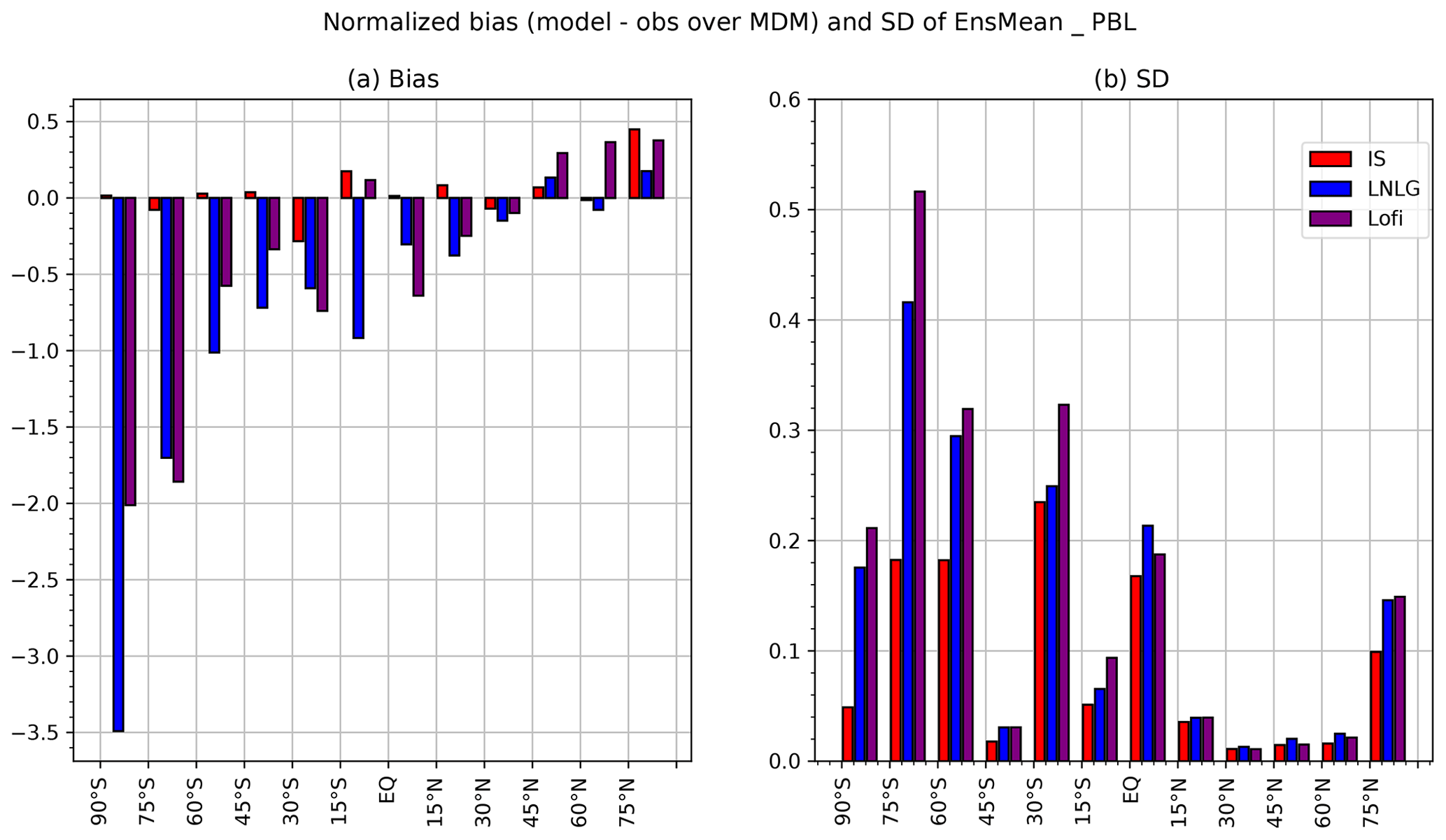
Figure 12Normalized bias (model minus observation divided by model data mismatch; MDM, see Sect. 2) in (a) and standard deviation in (b) for the ensemble mean of IS (in red), LNLGv9 (in blue), and LoFI (in purple). The evaluation is done by latitude and in the PBL. The data have been averaged over the 4 years of study (2015–2018).
3.4.1 Withheld in situ evaluation data
Here, we evaluate against the withheld in situ data introduced in Sect. 2.4.
Figure 12 shows the evaluation with the withheld data by latitude band for IS and LNLGv9. Over the Southern Hemisphere, a large underestimation of the ensemble mean of LNLGv9 appears compared to the observations. While biases are larger over the Southern Hemisphere they are smaller over the tropics. The large biases observed in LNLGv9 and not with the IS could be due to a latitudinal bias in the OCO-2 data. Going from the Southern to the Northern Hemisphere, we can see a change in the v9 biases, which go from underestimation to overestimation by the models. This behavior also appears in the IS but with lower biases (less than 0.5 for all latitudes). The variability between the models and observations is higher in the Southern Hemisphere than in the tropics and the northern latitudes (Fig. 12b). In addition, this same variability seems to be disproportional to the number of withheld data (see Fig. 2). Indeed, the standard deviation for both IS and LNLG is low when the number of withheld data is important (more than 10 000 data). Overall, the IS experiments are more consistent with the in situ measurements than the LNLG experiments are.

Figure 13Same as Fig. 12, but instead of an evaluation by latitude, the evaluation is by MIP region. No: northern; So: southern.
Figure 13 shows the normalized bias and standard deviation of the ensemble mean by MIP regions for LNLGv9 and IS. Evaluation by MIP regions reveals a different behavior than observed by latitudes. For instance, over temperate South America and northern tropical Africa, v9 has a larger underestimation than IS. Over Europe, we see here that v9 has smaller biases (less overestimation) than IS. Finally, if we look at southern tropical Africa, v9 is less biased than IS. Regarding the standard deviation, it seems that the three experiments have similarities but with closer agreement between IS and v9 for some regions.

Figure 14Normalized bias (a, b), normalized standard deviation (c, d), and root-mean-square error (RMSE in ppm; e, f) by latitudes for each model and for the IS experiment (a, c, e) and the LNLGv9 experiment (b, d, f).

Since the MDM values range over 2 orders of magnitude, the use of the normalized residuals gives the most meaningful interpretation of the residuals. When we look at the normalized bias and standard deviation for each model between IS and LNLGv9 experiments by latitudes (Fig. 14a, b, c, and d) and by MIP regions (Fig. 15a, b, c, and d), we can see this large difference with underestimation for all models assimilating v9 in the southern and tropical latitudes. This underestimation with all models is, however, generally not obtained with IS. When comparing the root-mean-square error (RMSE) between the models and the withheld data (Fig. 14e and f), we can observe a higher value for all models between 30 and 75∘ N with RMSE between 6 (4) and 10 ppm (7 ppm) for LNLG inversions (for IS inversions, respectively), while RMSE are below 3 ppm in the southern latitudes and in the tropics. These larger raw errors observed in the northern latitudes could come from the difference in the in situ network between northern and southern latitudes. Indeed, there are more measurements in the Northern Hemisphere close to regionally significant sources and sinks compared to other latitudinal bands (tropics and Southern Hemisphere). Compared to the ensemble mean, every model shows small normalized standard deviations across the latitudes, with values near 0.1 in the Northern Hemisphere and going from 0.2 to 0.6, according the models, between 75 to 60∘ S. However, the evaluation by MIP regions shows similarities between IS and v9 for all regions. This similarity is also found for the RMSE values (Fig. 15e and f) with however larger values for LNLG (maximum values of 10 ppm) than with IS (maximum of 8 ppm) over temperate North America, boreal Eurasia, boreal North America, Europe, and southern tropical Asia. Additionally, errors are larger for temperate North America than for temperate Eurasia as expected due to the sampling distribution. Normalizing the models with the MDM's values is equivalent to normalizing against this expected variability. We can also observe that some models do better at some latitudes and regions, while the others are better at other regions. However, the goals of the study are to envelop the uncertainty in the inversions, rather than ranking model performance.
3.4.2 ATom evaluation
Figure 16 shows the comparison of the posterior concentrations that were sampled at the locations and times of the ATom flight campaigns during 2015–2018. IS inversions overestimate CO2 concentrations for almost all latitudes and altitudes, with the exception of an underestimation between 30 and 60∘ N at low altitudes. On the other hand, LNLGv9 shows an underestimation at almost every latitude and gives larger biases than IS in general. This underestimation is consistent with the large underestimation observed, particularly in the Southern Hemisphere, with the withheld data (Fig. 14). In addition, for both experiments, we observe a large overestimation (with biases of 1 to 2 ppm) in the stratosphere of the boreal latitudes. This stratospheric region is affected by atmospheric circulation and has few observations to constrain the inversions. It is possible then that this excess of concentration, in both experiments, reflects the initial conditions of the inversion.
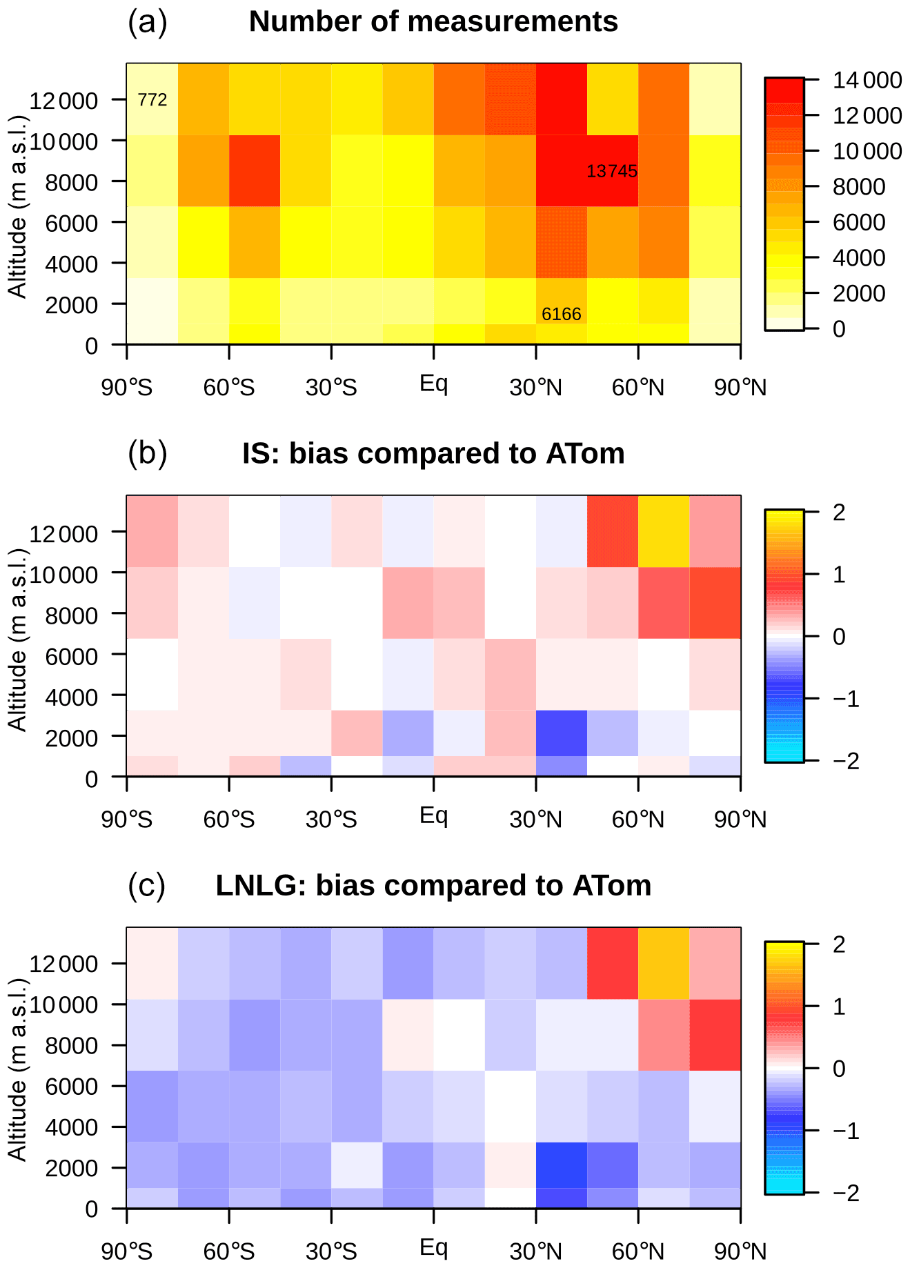
Figure 16Comparison between ATom measurement samples and the MIP ensemble for the IS and LNLG experiments. The ATom samples have been binned into five altitude levels (going from the ground to 14 km). Panel (a) shows the number of measurements for each bin. Panels (b) and (c) show, respectively, IS and LNLG experiment biases compared to ATom measurements. Biases are expressed in ppm CO2.
3.4.3 TCCON evaluation
Figure 17 shows bias and standard deviation for the prior, IS, and LNLGv9 experiments over all TCCON sites available during the 4 years of the study. We can observe that prior concentrations are biased high for almost all TCCON sites and all models. Compared to the evaluation of ISv7 in the study of Crowell et al. (2019), ISv9 and LNLGv9 biases are closer to each other (in the v7 MIP, the LNv7 were biased high compared to ISv7). Additionally, the OCO-2 biases have decreased (to values between −1.0 and 1.0 ppm) with v9 compared to v7, where biases ranged between −1.5 and 1.5 ppm (Crowell et al., 2019). As observed here as well, IS and v9 have large positive biases over most of the European sites, which could indicate either an issue related to the coarse resolution used by the transport models or to a latitudinal bias (though this is not shown here, positive biases are also observed for the East Trout Lake TCCON site situated in Canada at almost the same latitudinal band as the European sites). The Caltech, Saga, and Tenerife sites show large underestimation in both the IS and v9 results across all models. As mentioned and observed in v7 MIP, differences between the Caltech and Edwards sites (which are very close each other) could be due to the location of Edwards over the mountains and Caltech is affected in the Los Angeles Basin (Kort et al., 2012; Schwandner et al., 2017): the coarse resolution of models cannot differentiate the variability of these two sites (Crowell et al., 2019; Schuh et al., 2021). This could also explain the underestimation observed over Saga and Paris, which are urban regions. However, Saga is also a small island and could hence be influenced by ocean fluxes, where the assumed uncertainties are small compared to land. The underestimation observed for Izaña (Tenerife island) is probably linked to the same uncertainty (being a small island) but could also be due to the high altitude of the site. Finally, most sites over southern latitudinal bands are underestimated with LNLGv9 but slightly overestimated with IS, as also observed with the withheld in situ and ATom observations. However, Ascension Island, situated in the tropics, shows an overestimation of around 0.6 ppm for all models and for both IS and LNLGv9. This bias could be linked to the low density of data of this site compared to the other tropical sites (as observed in Fig. 3). The biases in v9 have decreased for Ascension Island compared to v7, where the biases were around 1.0 ppm for LN and LG.
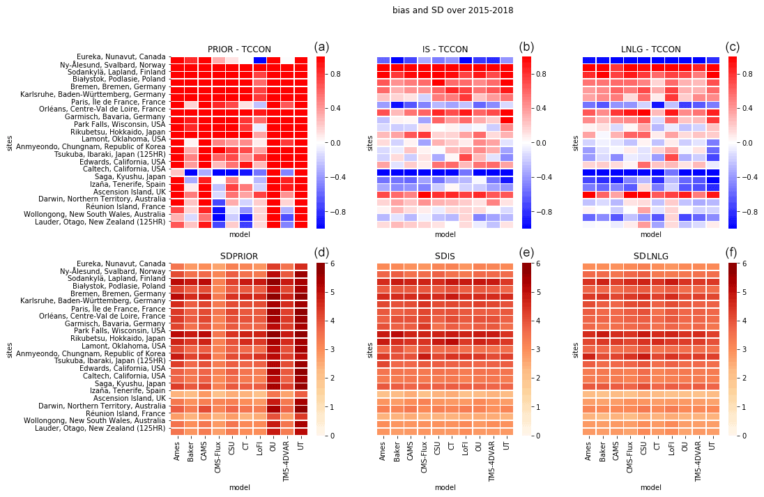
Figure 17Comparison between TCCON data and the MIP ensemble for the IS and LNLG experiments. Panels (a–c) show experiments biases and (d–f) show standard deviation compared to TCCON sites. Biases and standard deviation are expressed in ppm CO2. Priors are in (a, d), IS in (b, e), and LNLG in (c, f).
We have analyzed inversions assimilating OCO-2 version 9 XCO2 retrievals and compared them to in situ (IS) inversions, and to the OCO-2 v7 inversions. Our study is an update to the v7 MIP analysis of Crowell et al. (2019), which used OCO-2 v7 retrievals. In addition to comparing the LNLGv9 viewing mode inversion results to the IS ones, we also wanted to see if differences existed between an ensemble of atmospheric inverse models using either LNLGv9 or LNv7 and LGv7. We remind the reader that differences between XCO2 in v7 and v9 are not related to meteorology which is fixed, but to spectroscopy and geolocation improvements and better representation of aerosols (O'Dell et al., 2018). We have compared these different experiments, starting at the global scale, moving on to latitudinal scales, and finishing with regional scales. As expected, we did not find large differences between v7 and v9 at the global scale or latitudinal scale, except that the ensemble spread among the models was smaller with v9 than with v7. Transport model uncertainty is not expected to have changed dramatically since v7. This suggests that the reduction in the ensemble spread is likely related to a decrease in OCO-2 retrieval errors in v9 compared to v7.
However, posterior flux estimates between LNLGv9 and LNv7 and LGv7 differ for some regions. The key regions of interest that emerged from previous OCO-2 v7 MIP exercise and papers were in the tropics, including tropical Africa, tropical South America, and tropical Asia. The comparison between v7 and v9 for the northern tropical regions did not show large differences, except a small increase in carbon sources with v9 compared to v7 in northern tropical South America and a larger ensemble spread in southern tropical South America. Differences were also very small between v7 and v9 over tropical Asia. However, we have observed a change in the carbon cycle between v7 and v9 for southern tropical Africa, with a carbon sink with v7 and a carbon source with v9 during the El Niño period. Palmer et al. (2019) assimilated OCO-2 v7 land data and GOSAT v7 data separately during the El Niño period and analyzed the posterior emissions over the pan-tropical regions. With their inversions, they found carbon sources of 1.56 Pg C yr−1 in 2015 and 1.89 Pg C yr−1 in 2016 over the Northern Hemisphere of the tropics. The carbon sources they found with OCO-2 v7 are similar to what we obtain with our OCO-2 v9 inversions. Palmer et al. (2019) found with v7 that the largest seasonal cycle of carbon fluxes in the tropics was over northern tropical Africa. This analysis would have probably been similar with v9. However, while they had −0.21 Pg C yr−1 in 2015 and −0.12 Pg C yr−1 in 2016 over the southern tropical latitudes, we observe around 0.70 Pg C yr−1 in 2015 and 0.4 Pg C yr−1 in 2016 with v9 (Fig. 9). Analyzing our inversions at regional scales, we saw that this opposite sign in emissions was coming from southern tropical Africa. In our Fig. 11, we have been able to observe a source of around 0.25 Pg C yr−1 in 2015–2016, while v7 emissions were around −0.25 Pg C yr−1 for the same period, which is also what Palmer et al. (2019) found approximately. They concluded that the largest carbon uptake was over the northern Congo Basin, situated in the southern tropical Africa MIP region. This result and the difference between v7 and v9 suggest that the conclusion over the southern tropical Africa MIP region with v7 would have been different with v9. Liu et al. (2017) have assimilated OCO-2 v7 data to study the carbon cycle responses of the tropical regions to the 2015 El Niño and compared it to the 2011 La Niña. They found a respiration anomaly over tropical Africa, with an increased release of carbon of 0.6 Pg C yr−1 in 2015 compared to 2011. Gloor et al. (2018) did a similar study as Liu et al. (2017), but instead of comparing 2015 El Niño to 2011 La Niña, they compared the 2015 El Niño to the 1998 El Niño. Additionally, they did not assimilate satellite retrievals but rather in situ data from the NOAA surface station network. While their conclusions for southern tropical America and southern tropical Asia were similar to what Palmer et al. (2019) and Liu et al. (2017) found, they were surprised by their results over tropical Africa. Contrary to their expectations, Gloor et al. (2018) found hot conditions in the Congo Basin in February 2016 suggesting a release of carbon. Their results for the Congo Basin (with source of carbon) were in opposition with the previous papers, which found sinks of carbon during the El Niño period of 2015–2016. This anomaly over Africa was not expected, as Africa is generally not a tropical region affected by El Niño events. When Gloor et al. (2018) looked at the total-column carbon monoxide (CO) anomalies using MOPITT data, they found an anomalous flux in southern tropical Africa, with a large CO release in February 2016. Finally, they also found a water deficit at the beginning of 2016 (weaker than over the Amazon). We can then see that this study assimilating in situ measurements is in agreement with what we observe with v9 and our IS inversions. The corrections in the retrievals (in going from v7 to v9) hence seem to be important for CO2 emissions estimates, particularly over tropical regions.
In this study, we compare an ensemble of inversion models separately assimilating in situ data, OCO-2 v7 LN and LG retrievals, and OCO-2 v9 LNLG retrievals across the 2015–2018 period. Using the 4 years available with v9, in comparison to the two with v7, we have been able to observe better the impact of the El Niño period during 2015–2016 and the recovery period during the 2017–2018 period, especially over the tropics. Additionally, the ensemble spread among the models assimilating OCO-2 v9 retrievals is smaller for almost all regions compared to the ensemble spread with OCO-2 v7 retrievals, meaning either the impact of the long period used with the different models and priors or a better agreement in emissions among the models and the impact of the v9 retrieval bias correction. We find at the global scale a good agreement overall between fluxes inferred from the v7, v9, and in situ data. However, differences are found at smaller scales over northern latitudes and particularly over the tropics. While seasonality in the tropics differs significantly between the OCO-2 v7 and v9 compared to in situ results, the annual emissions show better agreement between the in situ data, LNv7, and v9, except over northern tropical Africa and northern tropical Asia. As was observed with v7, v9 also shows a stronger source of carbon over northern tropical Africa than that observed with in situ data. This weaker source given by the in situ data seems to be balanced over northern tropical Asia with a larger outgassing during the El Niño period that is not observed with the OCO-2 retrievals, as they show only sinks of carbon there for the whole period. It is difficult to conclude where these sources come from, as there are few in situ observations over this region. Finally, we see, as previously mentioned in several studies, a carbon uptake (of around −0.25 Pg C yr−1) over southern tropical Africa using the v7 data but a carbon release there using the v9 data of around 0.25 Pg C yr−1 during the El Niño period. The in situ data also suggest a carbon release. This difference between v7 and v9 over southern tropical Africa seems to show the impact of retrieval bias corrections on the regional CO2 fluxes, particularly in the tropics. This contradiction in the carbon budget conclusion between the two sets of OCO-2 inversions requires further investigation over this African region.
Evaluation with the withheld data, ATom aircraft measurements, and TCCON retrievals suggests similarities in biases between the in situ data and LNLGv9 data, with negative bias in the v9 OCO-2 data for almost all latitudes, particularly large in the Southern Hemisphere and slightly negative the tropics, where few evaluation data are available. Evaluation against TCCON also shows a reduction in retrieval errors with v9 ensemble models compared to v7.
Now that OCO-2 v10 retrievals are available, analysis and comparison between this new release and the two preceding ones presented in this study should bring further flux information and comparison for the tropical regions regarding retrieval corrections.
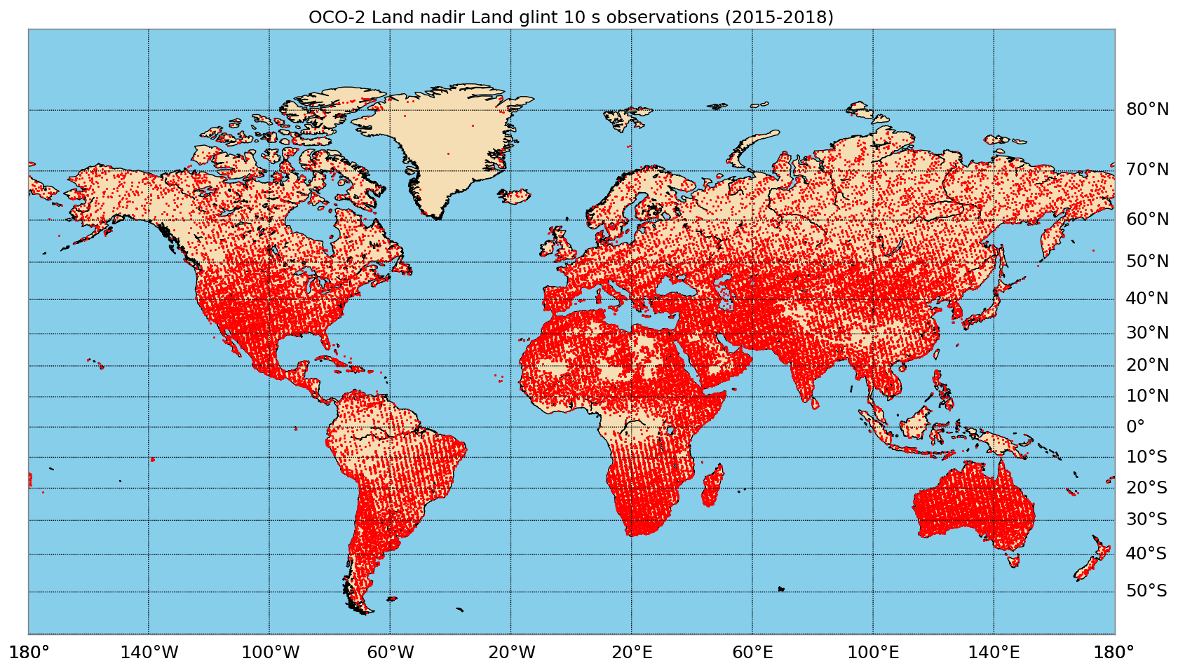
Figure A1Locations of OCO-2 land nadir and land glint 10 s retrievals for the period of study (2015 through 2018).
Further information including figures on individual models can be accessed using the following link https://gml.noaa.gov/ccgg/OCO2_v9mip/index.php (last access: September 2021).
B1 Ames
The Ames inversion system used the transport model GEOS-Chem (Goddard Earth Observing System – Chemistry; Bey et al., 2001), driven by meteorological parameters from the MERRA-2 reanalysis (Bosilovich et al., 2017) and run at a resolution (further description provided in Philip et al. (2019)). Surface fluxes were optimized monthly. The prior land biospheric CO2 fluxes (also called prior NEE) used in the model setup come from CarbonTracker CT2019 (Jacobson et al., 2020b) based on CASA-GFED4.1s (Potter et al., 1993; Giglio et al., 2013). The prior ocean fluxes are from the unoptimized CT2019 Ocean Inversion Fluxes prior (OIF) product (Jacobson et al., 2007, 2020a). Finally, prior emissions for fires are from GFED4.1s (Giglio et al., 2013; van der Werf et al., 2017). Prior NEE flux error was calculated as the range of five different biospheric CO2 flux models (CT2019-CASA-GFED4.1s, CASA-GFED3, NASA-CASA, Lund–Potsdam–Jena (LPJ), and Simple-Biosphere model version 4 (SiB-4))), scaled with 1.35 to represent unaccounted uncertainty components and keeping an upper bound of 5 times the absolute value of monthly prior NEE for each surface grid box of the model. The scaling was also done to get global total NEE uncertainty values in agreement with Global Carbon Project (GCP) estimates for the period of study (years 2015–2018). Oceanic prior flux error was assigned to be 5.0 times the absolute value of monthly oceanic prior fluxes in eachsurface grid box of the GEOS-Chem model. This scale factor was also done to get global total ocean uncertainty values in agreement with GCP estimates for 2015–2018. For both NEE and oceanic prior fluxes, no spatial or temporal correlations were considered.
B2 Baker
The transport model used in the Baker simulations is the Parameterized Chemical Transport Model (PCTM; Kawa et al., 2004). The meteorology fields come from the MERRA-2 reanalysis: these have been coarsened to a resolution of for the forward runs of the prior fluxes and to a resolution of for the assimilation of the measurements; the vertical resolution has been coarsened to 40 levels in both cases by grouping together the original 72 layers in the upper atmosphere. Biospheric priors come from the CASA-GFED3 (Potter et al., 1993; Randerson et al., 1997; van der Werf et al., 2004) and include gross primary productivity (GPP), net ecosystem respiration, wildfires, and biofuel emissions. A multiple of the respiration forward run is added onto the others to bring the global trend of CO2 at Mauna Loa into agreement with the observations across the 2014–2018 time span. The results shown are the mean of four separate inversions, each done using a different air–sea flux prior: (a) the NASA ocean biosphere model (NOBM; Gregg et al., 2003; Gregg and Casey, 2007), (b) the Takahashi et al. (2009) fluxes, (c) the Landschützer et al. (2015) fluxes, and (d) those same Landschützer et al. (2015) fluxes with a sink of 0.95 Pg C yr−1 added across the Southern Ocean. Uncertainties in the priors are based on Baker et al. (2006), with no correlations assumed between different weeks/grid boxes. Weekly fluxes are estimated using a variational data assimilation scheme (Baker et al., 2006).
B3 CAMS
CAMS simulation used the global general circulation model LMDz (Laboratoire de Météorologie Dynamique Zoom) with a spatial resolution of resolution and 39 vertical layers. The inferred fluxes are estimated in each horizontal grid point of the transport model with a temporal resolution of 8 d, separately for daytime and nighttime. ERA-Interim reanalysis meteorology fields are used. This inversion system is part of the PyVAR-CO2 configuration. Biospheric priors come from the climatology of the ORCHIDEE model version 4.6.9.5 (Krinner et al., 2005). Ocean priors are from the CMEMS (Denvil-Sommer et al., 2019). And fire priors are from GFED4 (Giglio et al., 2013; van der Werf et al., 2017).
The biospheric prior errors are assumed, over land, to dominate the error budget, and covariances are based on an analysis of mismatches with in situ flux measurements (Chevallier et al., 2006, 2012). Spatial correlations on daily mean NEE decay exponentially with a length of 500 km; standard deviations are set to 0.8 times the climatological daily-varying heterotrophic respiration flux simulated by ORCHIDEE, with a ceiling of 4 . Over a full year, the total 1σ uncertainty for the prior land fluxes amounts to about 3.0 Gt C yr−1.
Ocean prior uncertainty is defined as follows: (i) temporal correlations decay exponentially with a length of 1 month, (ii) unlike land, daytime, and nighttime flux errors are fully correlated, and (iii) spatial correlations follow an e-folding length of 1000 km; standard deviations are set to 0.1 .The global air–sea flux uncertainty is about 0.5 Gt C yr−1. Land and ocean flux errors are not correlated.
B4 CMS-Flux
Carbon Monitoring System (CMS)-Flux used a four-dimensional variational (4D-Var) inversion approach with the model GEOS-Chem. The model is driven by the Goddard Earth Observing System version 5 of the NASA Global Modeling Assimilation Office (GEOS-FP) meteorology and runs at a resolution. A net biospheric exchange (NBE) prior has been constructed using the CARDAMOM framework (Carbon Data Model Framework; Bloom et al., 2016). The CARDAMOM data assimilation system explicitly represents the time-resolved uncertainties in the NBE. The prior estimates are already constrained with multiple data streams accounting for measurement uncertainties following a Bayesian approach similar to that used in the four-dimensional variational approach. The CMS-Flux simulation uses the CARDAMOM setup as described by Bloom et al. (2016, 2020) resolved at monthly timescales; data constraints include GOME-2 solar-induced fluorescence (Joiner et al., 2013), MODIS leaf area index (LAI), and biomass and soil carbon. In addition, mean GPP and fire carbon emissions from 2010–2017 are constrained by FLUXCOM RS+METEO version 1 GPP (Tramontana et al., 2016; Jung et al., 2017) and GFEDv4.1 s (Randerson et al., 2012), respectively, both assimilated with an uncertainty of 20 %. The prior ocean error is 100 %. Fires are not optimized separately; they are part of the NBE. The Olsen and Randerson (2004) approach has been used to downscale monthly GPP and respiration fluxes to 3-hourly timescales, based on ERA-Interim reanalysis of global radiation and surface temperature. Fire fluxes are downscaled using the GFEDv4.1 daily- and diurnal-scale factors on monthly emissions. Posterior CARDAMOM NBE estimates are then summarized as NBE mean and standard deviation values. The NBE from CARDAMOM shows net carbon uptake of 2.3 Gt C yr−1 over the tropics and is close to neutral in the extra-tropics. The year-to-year variability (i.e., interannual variability, IAV) estimated from CARDAMOM from 2010–2017 is generally less than 0.1 outside of the tropics. Because of the weak interannual variability estimated by CARDAMOM, the same 2017 NBE prior is used for 2018. CARDAMOM generates uncertainty along with the mean state. The relative uncertainty over the tropics is generally larger than 100 %, and the magnitude is between 50 % and 100 % over the extra-tropics. We assume no correlation in the prior flux errors in either space or time.
B5 CSU
The CSU simulation used the GEOS-Chem model with a Bayesian synthesis technique. Transport was performed at resolution, and CO2 fluxes for both respiration and GPP were optimized at the TRANSCOM3 level as a function of plant functional type (PFT). The model is driven by MERRA-2 meteorology fields. Biospheric prior emissions are based on the Simple Biosphere Model Version 4 (SiB-4; Baker et al., 2013) at a resolution grid. SiB-4 is a land surface model that predicts vegetation and soil moisture, land surface energy, and terrestrial carbon cycle. It used carbon fluxes to determine biomass above and below the ground. Prior ocean comes from a climatology based on Landschützer v18. Prior standard deviations (independent, no prescribed correlations) for ocean exchange, respiration, and GPP were 10 % of the net exchange (or respiration or GPP). Fires are from GFED4.1s.
B6 CT
The CarbonTracker (CT) simulations presented here closely follow the methods used for CT2019B (Jacobson et al., 2020b), except that only one set of biosphere, wildfire, and oceanic emissions data was used. For the present experiments, first-guess land carbon emissions were provided by GFED4.1s (Giglio et al., 2013; van der Werf et al., 2017), and first-guess ocean emissions come from Jacobson et al. (2007). CT inversions optimize surface fluxes by estimating weekly scaling factors multiplying first-guess emissions for 156 ecoregions covering the globe. The optimization scheme is an ensemble Kalman filter with a 12-week assimilation window. Atmospheric transport is simulated by TM5 (Krol et al., 2005) with meteorology from the ERA-Interim reanalysis (Dee et al., 2011) with a global resolution of 3∘ longitude by 2∘ latitude and a zoom region over North America. Prior standard deviation is equivalent to 50 %. Prior covariance is applied such that the correlations between the same ecosystem types in different TRANSCOM regions decrease exponentially with distance scale L = 2000 km. More information can be found in https://gml.noaa.gov/ccgg/carbontracker/CT2019B_doc.php#tth_sEc8.2 (last access: September 2021).
B7 LoFI
While the OCO-2 MIP v7 (Crowell et al., 2019) was composed of models assimilating OCO-2 retrieval v7 or in situ data, the OCO-2 MIP v9 also has the model Low-order Flu Inversion (LoFI; Weir et al., 2021), which is an integrated Earth system model with data assimilation capabilities. LoFI (Weir et al., 2021) reproduces atmospheric and oceanic growth rates from a group of remote-sensing carbon fluxes. The model used is the Heracles 4.0 Goddard Earth Observing System (GEOS) general circulation model (GCM) including MERRA-2 meteorological inputs and a resolution grid with 72 vertical levels. Biospheric fluxes have a 3-hourly time step, while all other fluxes have a daily time step. Biospheric and biofuel priors come from the CASA-GFED3. Biomass burning priors are based on the Quick Fire Emissions Dataset (QFED; Darmenov and Silva, 2015). QFED is based on MODIS fire radiative power estimates using the technique from GFAS (Kaiser et al., 2012). Finally, oceanic priors are an extension of the Takahashi et al. (2009) climatology product used with NOAA zonal-mean surface CO2 and MERRA-2 wind speed. This approach is also used in the NOAA CarbonTracker system.
B8 OU
The OU simulation used the chemistry transport model TM5 (Krol et al., 2005) with a 4D-VAR assimilation algorithm. The model has been run at a resolution with 25 vertical layers. ERA-Interim meteorology fields are used here as well. Initial conditions are provided from CarbonTracker. Oceanic priors were constructed from Takahashi et al. (2009). Biospheric priors are based on CT2019 CASA-GFED3 and the fire prior from GFED3. Uncertainties are derived from different climatological fluxes. Exponential spatiotemporal correlation is assumed for the uncertainty in the prior flux. For the oceanic component, the length is 1000 km and the timescales is 3 weeks, while for the terrestrial component, length and timescale are 250 km and 1 week.
B9 TM5-4DVAR
The TM5-4DVAR simulation used the same transport model as the OU simulation with the same meteorological fields but on a resolution grid. A climatological average of CT2019 oceanic fluxes estimates constrained oceanic prior fluxes. Biospheric priors are taken from SiB CASA GFED4 (Van Der Velde et al., 2013) and fire priors from GFED4 (Randerson et al., 2012). The uncertainties in the biospheric prior are fixed to 0.5 times the heterotrophic respiration from SiB CASA. For the oceanic prior, the uncertainties are fixed at 1.57 times the absolute flux at each grid cell and time step. The same correlation, length, and timescale as the OU simulation are assumed and used in this TM5-4DVAR simulation.
B10 UT
The GEOS-Chem model has been used in the UT simulation, driven by assimilated meteorological observation from GEOS-FP and used with the 4D-Var assimilation algorithm. The model is run at resolution with 47 vertical layers. More information can be found in Deng et al. (2016). Fire priors are based on GFED4. Oceanic prior fluxes are based on the monthly climatology of Takahashi et al. (2009). And finally, biospheric priors are based on 3-hourly fluxes from the Boreal Ecosystem Productivity Simulator (Chen et al., 2012). Annual terrestrial ecosystem exchange is assumed to be neutral in each grid box (Deng and Chen, 2011; Deng et al., 2014). Optimized scaling factors are estimated with a monthly temporal resolution. Uncertainty is assumed to be 38 % for the fire emissions in each month and each model grid box, while it is 44 % for the ocean emissions and 22 % for terrestrial emissions.
The surface gridded flux are available from https://www.esrl.noaa.gov/gmd/ccgg/OCO2_v9mip/ (NOAA, 2019a). The in situ measurements are available from https://www.esrl.noaa.gov/gmd/ccgg/obspack/ (NOAA, 2019b). The TCCON data were obtained from the TCCON Data Archive hosted by CaltechDATA at https://tccondata.org (TCCON, 2019).
HP completed the analysis of the results, wrote the paper, and produced the figures. SC, DB, AS, SB, AJ, FC, FD, JL, MJ, SP, and BW provided surface flux estimates. DB provided the OCO-2 10 s averages. AJ provided in situ observations for assimilation, the withheld data for evaluation, and ATom figures. SB produced the quality-controlled TCCON time-averaged data. COD, DC, and AE provided feedback on the paper. SC, DB, AS, AJ, FC, FD, JL, MJ, SP, IB, and BW reviewed and commented on the final paper.
The contact author has declared that neither they nor their co-authors have any competing interests.
Publisher's note: Copernicus Publications remains neutral with regard to jurisdictional claims in published maps and institutional affiliations.
We thank TCCON PIs for the TCCON measurements at Eureka, Ny-Ålesund, Sodankylä, Białystok, Bremen, Karlsruhe, Paris, Orléans, Garmisch, Park Falls, Rikubetsu, Lamont, Anmeyondo, Tsukuba, Edwards, Caltech, Saga, Izaña, Ascension Island, Darwin, Réunion island, Wollongong, and Lauder. Eureka measurements are made by the Canadian Network for the Detection of Atmospheric Change (CANDAC) and in part by the Canadian Arctic ACE Validation Campaigns. They are supported by the Atlantic Innovation Fund/Nova Scotia Research Innovation Trust, Canada Foundation for Innovation, Canadian Foundation for Climate and Atmospheric Sciences, Canadian Space Agency, Environment Canada, Government of Canada International Polar Year funding, Natural Sciences and Engineering Research Council, Northern Scientific Training Program, Ontario Innovation Trust, Ontario Research Fund, and Polar Continental Shelf Program. Observations for Białystok are funded by the European Union (EU) projects InGOS and ICOS-INWIRE and by the Senate of Bremen. Local support for Bremen and Ny-Ålesund is provided by the EU projects InGOS and ICOS-INWIRE (26188, 36677, 284274, 313169, and 640276) and by the Senate of Bremen. Orléans observations are supported by the EU projects InGOS and ICOS-INWIRE, by the Senate of Bremen, and by the RAMCES team at LSCE. The Réunion island TCCON site is operated by the Royal Belgian Institute for Space Aeronomy with financial support since 2014 from the EU project ICOS-INWIRE and the ministerial decree for ICOS (FR/35/IC1 to FR/35/IC5) and local activities supported by LACy/UMR8105 – Université de La Réunion. The Paris TCCON site has received funding from Sorbonne Université, the French research center CNRS, the French space agency CNES, and Région Île-de-France. Garmisch funding was provided by the EU within the InGOS project. The Park Falls, Lamont, Edwards, and Caltech TCCON sites have received funding from National Aeronautics and Space Administration (NASA) grants NNX14AI60G, NNX11AG01G, NAG5-12247, and NNG05-GD07G and the NASA Orbiting Carbon Observatory Program. They are supported in part by the OCO-2 project. The TCCON stations at Rikubetsu and Tsukuba are supported in part by the GOSAT series project. Darwin and Wollongong TCCON stations are funded by NASA grants NAG5-12247 and NNG05-GD07G and supported by the Australian Research Council (ARC) grants DP140101552, DP110103118, DP0879468, and LP0562346. The Lauder TCCON site has received funding from National Institute of Water and Atmospheric (NIWA) Research through New Zealand's Ministry of Business, Innovation and Employment. We also acknowledge the NASA ATom aircraft-campaign data from the NASA Ames Earth Science Project Office (https://espo.nasa.gov/atom, last access: August 2020).
Part of this research has been supported by the NASA OCO-2 science team (grant no. 80NSSC18K0896) for David F. Baker, Sean Crowell, Hélène Peiro, and Andrew R. Jacobson, the NASA GeoCarb mission (grant no. 80LARC17C0001) for Sean Crowell, the OCO-2 ST proposal (2017) no. 80NSSC18K1312 for Andrew Schuh, and the Copernicus Atmosphere Monitoring Service, implemented by the European Centre for Medium-Range Weather Forecasts on behalf of the European Commission (grant no. CAMS73), for Frédéric Chevallier. In addition, Frédéric Chevallier was granted access to the HPC resources of TGCC under the allocation A0110102201 made by GENCI. Another part of the research was carried out at the Jet Propulsion Laboratory, California Institute of Technology, under a contract with the National Aeronautics and Space Administration (80NM0018D0004) (Junjie Liu). Sajeev Philip acknowledges financial support of the NASA Academic Mission Services by Universities Space Research Association at NASA Ames Research Center. Matthew Johnson acknowledges the internal funding from NASA's Earth Science Research and Analysis Program. Part of this study has been also supported by the OCO Missions, grant nos. 80NSSC18K1311 and 80NSSC20K0818 (Sourish Basu), and the NASA's Carbon Monitoring System (NNH16DA001N-CMS 16-CMS16-0054) and Science Team for the OCO Missions (NNH17ZDA001N-OCO2 17-OCO2-17-0010) (Brad Weir).
This paper was edited by Michel Van Roozendael and reviewed by two anonymous referees.
Baker, D. F., Doney, S. C., and Schimel, D. S.: Variational data assimilation for atmospheric CO2, Tellus B, 58, 359–365, https://doi.org/10.1111/j.1600-0889.2006.00218.x, 2006. a, b
Baker, D. F., Bell, E., Davis, K. J., Campbell, J. F., Lin, B., and Dobler, J.: A new exponentially-decaying error correlation model for assimilating OCO-2 column-average CO2 data, using a length scale computed from airborne lidar measurements, Geosci. Model Dev. Discuss. [preprint], https://doi.org/10.5194/gmd-2020-444, in review, 2021. a, b
Basu, S., Guerlet, S., Butz, A., Houweling, S., Hasekamp, O., Aben, I., Krummel, P., Steele, P., Langenfelds, R., Torn, M., Biraud, S., Stephens, B., Andrews, A., and Worthy, D.: Global CO2 fluxes estimated from GOSAT retrievals of total column CO2, Atmos. Chem. Phys., 13, 8695–8717, https://doi.org/10.5194/acp-13-8695-2013, 2013. a, b
Basu, S., Baker, D. F., Chevallier, F., Patra, P. K., Liu, J., and Miller, J. B.: The impact of transport model differences on CO2 surface flux estimates from OCO-2 retrievals of column average CO2, Atmos. Chem. Phys., 18, 7189–7215, https://doi.org/10.5194/acp-18-7189-2018, 2018. a, b
Bey, I., Jacob, D. J., Yantosca, R. M., Logan, J. A., Field, B. D., Fiore, A. M., Li, Q., Liu, H. Y., Mickley, L. J., and Schultz, M. G.: Global modeling of tropospheric chemistry with assimilated meteorology: Model description and evaluation, J. Geophys. Res.-Atmos., 106, 23073–23095, https://doi.org/10.1029/2001JD000807, 2001. a
Bloom, A. A., Exbrayat, J. F., Van Der Velde, I. R., Feng, L., and Williams, M.: The decadal state of the terrestrial carbon cycle: Global retrievals of terrestrial carbon allocation, pools, and residence times, P. Natl. Acad. Sci. USA, 113, 1285–1290, https://doi.org/10.1073/pnas.1515160113, 2016. a, b
Bloom, A. A., Bowman, K. W., Liu, J., Konings, A. G., Worden, J. R., Parazoo, N. C., Meyer, V., Reager, J. T., Worden, H. M., Jiang, Z., Quetin, G. R., Smallman, T. L., Exbrayat, J.-F., Yin, Y., Saatchi, S. S., Williams, M., and Schimel, D. S.: Lagged effects regulate the inter-annual variability of the tropical carbon balance, Biogeosciences, 17, 6393–6422, https://doi.org/10.5194/bg-17-6393-2020, 2020. a
Blumenstock, T., Hase, F., Schneider, M., García, O. E., and Sepúlveda, E.: TCCON data from Izana (ES), Release GGG2014.R1, https://doi.org/10.14291/TCCON.GGG2014.IZANA01.R1, 2017. a
Bosilovich, M. G., Robertson, F. R., Takacs, L., Molod, A., and Mocko, D.: Atmospheric water balance and variability in the MERRA-2 reanalysis, J. Climate, 30, 1177–1196, https://doi.org/10.1175/JCLI-D-16-0338.1, 2017. a
Chen, J. M., Mo, G., Pisek, J., Liu, J., Deng, F., Ishizawa, M., and Chan, D.: Effects of foliage clumping on the estimation of global terrestrial gross primary productivity, Global Biogeochem. Cy., 26, 1–18, https://doi.org/10.1029/2010GB003996, 2012. a, b
Chevallier, F., Engelen, R. J., and Peylin, P.: The contribution of AIRS data to the estimation of CO2 sources and sinks, Geophys. Res. Lett., 32, 1–4, https://doi.org/10.1029/2005GL024229, 2005. a
Chevallier, F., Viovy, N., Reichstein, M., and Ciais, P.: On the assignment of prior errors in Bayesian inversions of CO2 surface fluxes, Geophys. Res. Lett., 33, 1–5, https://doi.org/10.1029/2006GL026496, 2006. a
Chevallier, F., Fortems, A., Bousquet, P., Pison, I., Szopa, S., Devaux, M., and Hauglustaine, D. A.: African CO emissions between years 2000 and 2006 as estimated from MOPITT observations, Biogeosciences, 6, 103–111, https://doi.org/10.5194/bg-6-103-2009, 2009. a
Chevallier, F., Feng, L., Bösch, H., Palmer, P. I., and Rayner, P. J.: On the impact of transport model errors for the estimation of CO2 surface fluxes from GOSAT observations, Geophys. Res. Lett., 37, 1–5, https://doi.org/10.1029/2010GL044652, 2010. a
Chevallier, F., Wang, T., Ciais, P., Maignan, F., Bocquet, M., Altaf Arain, M., Cescatti, A., Chen, J., Dolman, A. J., Law, B. E., Margolis, H. A., Montagnani, L., and Moors, E. J.: What eddy-covariance measurements tell us about prior land flux errors in CO2-flux inversion schemes, Global Biogeochem. Cy., 26, 1–9, https://doi.org/10.1029/2010GB003974, 2012. a
Chevallier, F., Palmer, P. I., Feng, L., Boesch, H., O'Dell, C. W., and Bousquet, P.: Toward robust and consistent regional CO2 flux estimates from in situ and spaceborne measurements of atmospheric CO2, Geophys. Res. Lett., 41, 1065–1070, https://doi.org/10.1002/2013GL058772, 2014. a, b, c, d
Chevallier, F., Remaud, M., O'Dell, C. W., Baker, D., Peylin, P., and Cozic, A.: Objective evaluation of surface- and satellite-driven carbon dioxide atmospheric inversions, Atmos. Chem. Phys., 19, 14233–14251, https://doi.org/10.5194/acp-19-14233-2019, 2019. a
Ciais, P., Rayner, P., Chevallier, F., Bousquet, P., Logan, M., Peylin, P., and Ramonet, M.: Atmospheric inversions for estimating CO2 fluxes: Methods and perspectives, Climatic Change, 103, 69–92, https://doi.org/10.1007/s10584-010-9909-3, 2010. a
Ciais, P., Sabine, C., Bala, G., Bopp, L., Brovkin, V., Canadell, J., Chhabra, A., DeFries, R., Galloway, J., Heimann, M., Jones, C., Quéré, C. L., Myneni, R., Piao, S., and Thornton, P.: The physical science basis. Contribution of working group I to the fifth assessment report of the intergovernmental panel on climate change, Change, IPCC Climate, 465–570, https://doi.org/10.1017/CBO9781107415324.015, 2013. a
Connor, B. J., Boesch, H., Toon, G., Sen, B., Miller, C., and Crisp, D.: Orbiting Carbon Observatory: Inverse method and prospective error analysis, J. Geophys. Res.-Atmos., 113, 1–14, https://doi.org/10.1029/2006JD008336, 2008. a
Cooperative Global Atmospheric Data Integration Project: Multi-laboratory compilation of atmospheric carbon dioxide data for the period 1957–2018; {obspack_co2_1_GLOBALVIEWplus_v5.0_2019_08_12}, https://doi.org/10.25925/20190812, 2019. a
Crisp, D., Pollock, H. R., Rosenberg, R., Chapsky, L., Lee, R. A. M., Oyafuso, F. A., Frankenberg, C., O'Dell, C. W., Bruegge, C. J., Doran, G. B., Eldering, A., Fisher, B. M., Fu, D., Gunson, M. R., Mandrake, L., Osterman, G. B., Schwandner, F. M., Sun, K., Taylor, T. E., Wennberg, P. O., and Wunch, D.: The on-orbit performance of the Orbiting Carbon Observatory-2 (OCO-2) instrument and its radiometrically calibrated products, Atmos. Meas. Tech., 10, 59–81, https://doi.org/10.5194/amt-10-59-2017, 2017. a, b, c
Crowell, S., Baker, D., Schuh, A., Basu, S., Eldering, A., Feng, L., Crisp, D., O'Dell, C. W., Oda, T., Sweeney, C., Palmer, P. I., and Jones, D. B. A.: The 2015–2016 carbon cycle as seen from OCO-2 and the global in situ network, Atmos. Chem. Phys., 19, 9797–9831, https://doi.org/10.5194/acp-19-9797-2019, 2019. a, b, c, d, e, f, g, h, i, j, k, l, m, n, o, p, q, r, s, t, u, v, w, x, y, z, aa
Darmenov, A. S. and Silva, A.: The Quick Fire Emissions Dataset (QFED): Documentation of versions 2.1, 2.2 and 2.4, NASA Technical Report Series on Global Modeling and Data Assimilation, NASA/TM-2015-104606, vol. 38, Document ID: 20180005253, 11–25, 2015. a
Dee, D. P., Uppala, S. M., Simmons, A. J., Berrisford, P., Poli, P., Kobayashi, S., Andrae, U., Balmaseda, M. A., Balsamo, G., Bauer, P., Bechtold, P., Beljaars, A. C., van de Berg, L., Bidlot, J., Bormann, N., Delsol, C., Dragani, R., Fuentes, M., Geer, A. J., Haimberger, L., Healy, S. B., Hersbach, H., Hólm, E. V., Isaksen, L., Kållberg, P., Köhler, M., Matricardi, M., Mcnally, A. P., Monge-Sanz, B. M., Morcrette, J. J., Park, B. K., Peubey, C., de Rosnay, P., Tavolato, C., Thépaut, J. N., and Vitart, F.: The ERA-Interim reanalysis: Configuration and performance of the data assimilation system, Q. J. Roy. Meteor. Soc., 137, 553–597, https://doi.org/10.1002/qj.828, 2011. a
De Mazière, M., Sha, M. K., Desmet, F., Hermans, C., Scolas, F., Kumps, N., Metzger, J.-M., Duflot, V., and Cammas, J.-P.: TCCON data from Réunion Island (RE), Release GGG2014.R1, https://doi.org/10.14291/TCCON.GGG2014.REUNION01.R1, 2017. a
Deng, F. and Chen, J. M.: Recent global CO2 flux inferred from atmospheric CO2 observations and its regional analyses, Biogeosciences, 8, 3263–3281, https://doi.org/10.5194/bg-8-3263-2011, 2011. a
Deng, F., Jones, D. B. A., Henze, D. K., Bousserez, N., Bowman, K. W., Fisher, J. B., Nassar, R., O'Dell, C., Wunch, D., Wennberg, P. O., Kort, E. A., Wofsy, S. C., Blumenstock, T., Deutscher, N. M., Griffith, D. W. T., Hase, F., Heikkinen, P., Sherlock, V., Strong, K., Sussmann, R., and Warneke, T.: Inferring regional sources and sinks of atmospheric CO2 from GOSAT XCO2 data, Atmos. Chem. Phys., 14, 3703–3727, https://doi.org/10.5194/acp-14-3703-2014, 2014. a, b
Deng, F., Jones, D. B. A., Dell, C. W. O., Nassar, R., and Parazoo, N. C.: Combining GOSAT XCO2 observations over land and ocean to improve regional CO2 flux estimates, J. Geophys. Res.-Atmos., 121, 1896–1913, https://doi.org/10.1002/2015JD024157, 2016. a
Denvil-Sommer, A., Gehlen, M., Vrac, M., and Mejia, C.: LSCE-FFNN-v1: a two-step neural network model for the reconstruction of surface ocean pCO2 over the global ocean, Geosci. Model Dev., 12, 2091–2105, https://doi.org/10.5194/gmd-12-2091-2019, 2019. a
Deutscher, N. M., Notholt, J., Messerschmidt, J., Weinzierl, C., Warneke, T., Petri, C., and Grupe, P.: TCCON data from Bialystok (PL), Release GGG2014.R2, https://doi.org/10.14291/TCCON.GGG2014.BIALYSTOK01.R2, 2019. a
DiGangi, J., Choi, Y., Nowak, J., Halliday, H., Yang, M., Baier, B., and Sweeney, C.: ACT-America: L2 In Situ Atmospheric CO2, CO, CH4, and O3 Concentrations, Eastern USA, ORNL DAAC, Oak Ridge, Tennessee, USA, https://doi.org/10.3334/ORNLDAAC/1556, 2018. a, b
Eldering, A., O'Dell, C. W., Wennberg, P. O., Crisp, D., Gunson, M. R., Viatte, C., Avis, C., Braverman, A., Castano, R., Chang, A., Chapsky, L., Cheng, C., Connor, B., Dang, L., Doran, G., Fisher, B., Frankenberg, C., Fu, D., Granat, R., Hobbs, J., Lee, R. A. M., Mandrake, L., McDuffie, J., Miller, C. E., Myers, V., Natraj, V., O'Brien, D., Osterman, G. B., Oyafuso, F., Payne, V. H., Pollock, H. R., Polonsky, I., Roehl, C. M., Rosenberg, R., Schwandner, F., Smyth, M., Tang, V., Taylor, T. E., To, C., Wunch, D., and Yoshimizu, J.: The Orbiting Carbon Observatory-2: first 18 months of science data products, Atmos. Meas. Tech., 10, 549–563, https://doi.org/10.5194/amt-10-549-2017, 2017. a, b
Enting, I. G.: Inverse Problems in Atmospheric Constituent Transport, Cambridge Atmospheric and Space Science Series, Cambridge University Press, https://doi.org/10.1017/CBO9780511535741, 2002. a
Enting, I. G. and Newsam, G. N.: Atmospheric constituent inversion problems: Implications for baseline monitoring, J. Atmos. Chem., 11, 69–87, https://doi.org/10.1007/BF00053668, 1990. a
Feist, D. G., Arnold, S. G., John, N., and Geibel, M. C.: TCCON data from Ascension Island (SH), Release GGG2014R0, TCCON data archive, CaltechDATA, https://doi.org/10.14291/tccon.ggg2014.ascension01.R0/1149285, 2014. a
Feng, L., Palmer, P. I., Parker, R. J., Deutscher, N. M., Feist, D. G., Kivi, R., Morino, I., and Sussmann, R.: Estimates of European uptake of CO2 inferred from GOSAT retrievals: sensitivity to measurement bias inside and outside Europe, Atmos. Chem. Phys., 16, 1289–1302, https://doi.org/10.5194/acp-16-1289-2016, 2016. a, b, c
Field, R. D., Van Der Werf, G. R., Fanin, T., Fetzer, E. J., Fuller, R., Jethva, H., Levy, R., Livesey, N. J., Luo, M., Torres, O., and Worden, H. M.: Indonesian fire activity and smoke pollution in 2015 show persistent nonlinear sensitivity to El Niño-induced drought, P. Natl. Acad. Sci. USA, 113, 9204–9209, https://doi.org/10.1073/pnas.1524888113, 2016. a
Friedlingstein, P., O'Sullivan, M., Jones, M. W., Andrew, R. M., Hauck, J., Olsen, A., Peters, G. P., Peters, W., Pongratz, J., Sitch, S., Le Quéré, C., Canadell, J. G., Ciais, P., Jackson, R. B., Alin, S., Aragão, L. E. O. C., Arneth, A., Arora, V., Bates, N. R., Becker, M., Benoit-Cattin, A., Bittig, H. C., Bopp, L., Bultan, S., Chandra, N., Chevallier, F., Chini, L. P., Evans, W., Florentie, L., Forster, P. M., Gasser, T., Gehlen, M., Gilfillan, D., Gkritzalis, T., Gregor, L., Gruber, N., Harris, I., Hartung, K., Haverd, V., Houghton, R. A., Ilyina, T., Jain, A. K., Joetzjer, E., Kadono, K., Kato, E., Kitidis, V., Korsbakken, J. I., Landschützer, P., Lefèvre, N., Lenton, A., Lienert, S., Liu, Z., Lombardozzi, D., Marland, G., Metzl, N., Munro, D. R., Nabel, J. E. M. S., Nakaoka, S.-I., Niwa, Y., O'Brien, K., Ono, T., Palmer, P. I., Pierrot, D., Poulter, B., Resplandy, L., Robertson, E., Rödenbeck, C., Schwinger, J., Séférian, R., Skjelvan, I., Smith, A. J. P., Sutton, A. J., Tanhua, T., Tans, P. P., Tian, H., Tilbrook, B., van der Werf, G., Vuichard, N., Walker, A. P., Wanninkhof, R., Watson, A. J., Willis, D., Wiltshire, A. J., Yuan, W., Yue, X., and Zaehle, S.: Global Carbon Budget 2020, Earth Syst. Sci. Data, 12, 3269–3340, https://doi.org/10.5194/essd-12-3269-2020, 2020. a, b
Giglio, L., Randerson, J. T., and Van Der Werf, G. R.: Analysis of daily, monthly, and annual burned area using the fourth-generation global fire emissions database (GFED4), J. Geophys. Res.-Biogeo., 118, 317–328, https://doi.org/10.1002/jgrg.20042, 2013. a, b, c, d, e
Gloor, E., Wilson, C., Chipperfield, M. P., Chevallier, F., Buermann, W., Boesch, H., Parker, R., Somkuti, P., Gatti, L. V., Correia, C., Domingues, L. G., Peters, W., Miller, J., Deeter, M. N., and Sullivan, M. J.: Tropical land carbon cycle responses to 2015/16 El Niño as recorded by atmospheric greenhouse gas and remote sensing data, Philos. T. Roy. Soc. B, 373, 1760, https://doi.org/10.1098/rstb.2017.0302, 2018. a, b, c
Goo, T.-Y., Oh, Y.-S., and Velazco, V. A.: TCCON data from Anmeyondo (KR), Release GGG2014R0, TCCON data archive, CaltechDATA, https://doi.org/10.14291/tccon.ggg2014.anmeyondo01.R0/1149284, 2014. a
Gregg, W. W. and Casey, N. W.: Modeling coccolithophores in the global oceans, Deep-Sea Res. Pt. II, 54, 447–477, https://doi.org/10.1016/j.dsr2.2006.12.007, 2007. a
Gregg, W. W., Ginoux, P., Schopf, P. S., and Casey, N. W.: Phytoplankton and iron: validation of a global three-dimensional ocean biogeochemical model, Deep-Sea Res. Pt. II, 50, 3143–3169, https://doi.org/10.1016/j.dsr2.2003.07.013, 2003. a
Griffith, D. W. T., Deutscher, N. M., Velazco, V. A., Wennberg, P. O., Yavin, Y., Aleks, G. K., Washenfelder, R. a., Toon, G. C., Blavier, J.-F., Murphy, C., Jones, N., Kettlewell, G., Connor, B. J., Macatangay, R., Roehl, C., Ryczek, M., Glowacki, J., Culgan, T., and Bryant, G.: TCCON data from Darwin (AU), Release GGG2014R0, TCCON data archive, CaltechDATA, https://doi.org/10.14291/tccon.ggg2014.darwin01.R0/1149290, 2014a. a
Griffith, D. W. T., Velazco, V. A., Deutscher, N. M., Murphy, C., Jones, N., Wilson, S., Macatangay, R., Kettlewell, G., Buchholz, R. R., and Riggenbach, M.: TCCON data from Wollongong (AU), Release GGG2014R0, TCCON data archive, CaltechDATA, https://doi.org/10.14291/tccon.ggg2014.wollongong01.R0/1149291, 2014b. a
Gurney, K. R., Law, R. M., Denning, A. S., Rayner, P. J., Baker, D., Bousquet, P., Bruhwiler, L., Chen, Y. H., Ciais, P., Fan, S., Fung, I. Y., Gloor, M., Heimann, M., Higuchi, K., John, J., Maki, T., Maksyutov, S., Masarie, K., Peylin, P., Prather, M., Pak, B. C., Randerson, J., Sarmiento, J., Taguchi, S., Takahashi, T., and Yuen, C. W.: Towards robust regional estimates of annual mean CO2 sources and sinks, Nature, 415, 626–630, 2002. a
Hase, F., Blumenstock, T., Dohe, S., Groß, J., and Kiel, M.: TCCON data from Karlsruhe (DE), Release GGG2014.R1, 10.14291/TCCON.GGG2014.KARLSRUHE01.R1/1182416, 2015. a
Houghton, R. A., Butman, D., Bunn, A. G., Krankina, O. N., Schlesinger, P., and Stone, T. A.: Mapping Russian forest biomass with data from satellites and forest inventories, Environ. Res. Lett., 2, 4, https://doi.org/10.1088/1748-9326/2/4/045032, 2007. a
Houweling, S., Baker, D., Basu, S., Boesch, H., Butz, A., Chevallier, F., Deng, F., Dlugokencky, E. J., Feng, L., Ganshin, A., Hasekamp, O., Jones, D., Maksyutov, S., Marshall, J., Oda, T., O'Dell, C. W., Oshchepkov, S., Palmer, P. I., Peylin, P., Poussi, Z., Reum, F., Takagi, H., Yoshida, Y., and Zhuravlev, R.: An intercomparison of inversemodels for estimating sources and sinks of CO2 using GOSAT measurements, J. Geophys. Res., 120, 5253–5266, https://doi.org/10.1002/2014JD022962, 2015. a, b, c, d, e
Iraci, L. T., Podolske, J., Hillyard, P. W., Roehl, C., Wennberg, P. O., Blavier, J.-F., Allen, N., Wunch, D., Osterman, G. B., and Albertson, R.: TCCON data from Edwards (US), Release GGG2014R1, TCCON data archive, CaltechDATA, https://doi.org/10.14291/tccon.ggg2014.edwards01.R1/1255068, 2016. a
Jacobson, A. R., Fletcher, S. E., Gruber, N., Sarmiento, J. L., and Gloor, M.: A joint atmosphere-ocean inversion for surface fluxes of carbon dioxide: 1. Methods and global-scale fluxes, Global Biogeochem. Cy., 21, GB1019, https://doi.org/10.1029/2005GB002556, 2007. a, b
Jacobson, A. R., Schuldt, K. N., Miller, J. B., Oda, T., Tans, P., Andrews, A., Mund, J., Ott, L., Collatz, G. J., Aalto, T., Afshar, S., Aikin, K., Aoki, S., Apadula, F., Baier, B., Bergamaschi, P., Beyersdorf, A., Biraud, S. C., Bollenbacher, A., Bowling, D., Brailsford, G., and Zimnoch, M.: Carbontracker CT2019, Model published 2020 by NOAA Earth System Research Laboratory, Global Monitoring Division, https://doi.org/10.25925/39m3-6069, 2020a. a, b
Jacobson, A. R., Schuldt, K. N., Miller, J. B., Oda, T., Tans, P., Arlyn Andrews, Mund, J., Ott, L., Collatz, G. J., Aalto, T., Afshar, S., Aikin, K., Aoki, S., Apadula, F., Baier, B., Bergamaschi, P., Beyersdorf, A., Biraud, S. C., Bollenbacher, A., Bowling, D., Brailsford, G., Abshire, J. B., Chen, G., Huilin Chen, Lukasz Chmura, Sites Climadat, Colomb, A., Conil, S., Cox, A., Cristofanelli, P., Cuevas, E., Curcoll, R., Sloop, C. D., Davis, K., Wekker, S. D., Delmotte, M., DiGangi, J. P., Dlugokencky, E., Ehleringer, J., Elkins, J. W., Emmenegger, L., Fischer, M. L., Forster, G., Frumau, A., Galkowski, M., Gatti, L. V., Gloor, E., Griffis, T., Hammer, S., Haszpra, L., Hatakka, J., Heliasz, M., Hensen, A., Hermanssen, O., Hintsa, E., Holst, J., Jaffe, D., Karion, A., Kawa, S. R., Keeling, R., Keronen, P., Kolari, P., Kominkova, K., Kort, E., Krummel, P., Kubistin, D., Labuschagne, C., Langenfelds, R., Laurent, O., Laurila, T., Lauvaux, T., Law, B., Lee, J., Lehner, I., Leuenberger, M., Levin, I., Levula, J., Lin, J., Lindauer, M., Loh, Z., Lopez, M., Luijkx, I. T., Myhre, C. L., Machida, T., Mammarella, I., Manca, G., Manning, A., Manning, A., Marek, M. V., Marklund, P., Martin, M. Y., Matsueda, H., McKain, K., Meijer, H., Meinhardt, F., Miles, N., Miller, C. E., Mölder, M., Montzka, S., Moore, F., Josep-Anton Morgui, Morimoto, S., Munger, B., Jaroslaw Necki, Newman, S., Nichol, S., Niwa, Y., O'Doherty, S., Mikaell Ottosson-Löfvenius, Paplawsky, B., Peischl, J., Peltola, O., Jean-Marc Pichon, Piper, S., Plass-Dölmer, C., Ramonet, M., Reyes-Sanchez, E., Richardson, S., Riris, H., Ryerson, T., Saito, K., Sargent, M., Sasakawa, M., Sawa, Y., Say, D., Scheeren, B., Schmidt, M., Schmidt, A., Schumacher, M., Shepson, P., Shook, M., Stanley, K., Steinbacher, M., Stephens, B., Sweeney, C., Thoning, K., Torn, M., Turnbull, J., Tørseth, K., Bulk, P. V. D., Dinther, D. V., Vermeulen, A., Viner, B., Vitkova, G., Walker, S., Weyrauch, D., Wofsy, S., Worthy, D., Dickon Young, and Miroslaw Zimnoch: CarbonTracker CT2019B, https://doi.org/10.25925/20201008, 2020b. a, b
Joiner, J., Guanter, L., Lindstrot, R., Voigt, M., Vasilkov, A. P., Middleton, E. M., Huemmrich, K. F., Yoshida, Y., and Frankenberg, C.: Global monitoring of terrestrial chlorophyll fluorescence from moderate-spectral-resolution near-infrared satellite measurements: methodology, simulations, and application to GOME-2, Atmos. Meas. Tech., 6, 2803–2823, https://doi.org/10.5194/amt-6-2803-2013, 2013. a
Jung, M., Reichstein, M., Schwalm, C. R., Huntingford, C., Sitch, S., Ahlström, A., Arneth, A., Camps-Valls, G., Ciais, P., Friedlingstein, P., Gans, F., Ichii, K., Jain, A. K., Kato, E., Papale, D., Poulter, B., Raduly, B., Rödenbeck, C., Tramontana, G., Viovy, N., Wang, Y. P., Weber, U., Zaehle, S., and Zeng, N.: Compensatory water effects link yearly global land CO2 sink changes to temperature, Nature, 541, 516–520, https://doi.org/10.1038/nature20780, 2017. a
Kaiser, J. W., Heil, A., Andreae, M. O., Benedetti, A., Chubarova, N., Jones, L., Morcrette, J.-J., Razinger, M., Schultz, M. G., Suttie, M., and van der Werf, G. R.: Biomass burning emissions estimated with a global fire assimilation system based on observed fire radiative power, Biogeosciences, 9, 527–554, https://doi.org/10.5194/bg-9-527-2012, 2012. a
Kawa, S. R., Erickson, I. J., Pawson, S., and Zhu, Z.: Global CO2 transport simulations using meteorological data from the NASA data assimilation system, J. Geophys. Res.-Atmos., 109, 1–17, https://doi.org/10.1029/2004JD004554, 2004. a
Kawakami, S., Ohyama, H., Arai, K., Okumura, H., Taura, C., Fukamachi, T., and Sakashita, M.: TCCON data from Saga (JP), Release GGG2014R0, TCCON data archive, CaltechDATA, https://doi.org/10.14291/tccon.ggg2014.saga01.R0/1149283, 2014. a
Kiel, M., O'Dell, C. W., Fisher, B., Eldering, A., Nassar, R., MacDonald, C. G., and Wennberg, P. O.: How bias correction goes wrong: measurement of XCO2 affected by erroneous surface pressure estimates, Atmos. Meas. Tech., 12, 2241–2259, https://doi.org/10.5194/amt-12-2241-2019, 2019. a, b, c
Kivi, R., Heikkinen, P., and Kyrö, E.: TCCON data from Sodankyla (FI), Release GGG2014R0, TCCON data archive, CaltechDATA, https://doi.org/10.14291/tccon.ggg2014.sodankyla01.R0/1149280, 2014. a
Kort, E. A., Frankenberg, C., Miller, C. E., and Oda, T.: Space-based observations of megacity carbon dioxide, Geophys. Res. Lett., 39, 1–5, https://doi.org/10.1029/2012GL052738, 2012. a
Krinner, G., Viovy, N., de Noblet-Ducoudré, N., Ogée, J., Polcher, J., Friedlingstein, P., Ciais, P., Sitch, S., and Prentice, I. C.: A dynamic global vegetation model for studies of the coupled atmosphere-biosphere system, Global Biogeochem. Cy., 19, 1–33, https://doi.org/10.1029/2003GB002199, 2005. a
Krol, M., Houweling, S., Bregman, B., van den Broek, M., Segers, A., van Velthoven, P., Peters, W., Dentener, F., and Bergamaschi, P.: The two-way nested global chemistry-transport zoom model TM5: algorithm and applications, Atmos. Chem. Phys., 5, 417–432, https://doi.org/10.5194/acp-5-417-2005, 2005. a, b
Kuze, A., Suto, H., Nakajima, M., and Hamazaki, T.: Initial Onboard Performance of TANSO-FTS on GOSAT, in: Advances in Imaging, FTuC2, Optical Society of America, https://doi.org/10.1364/FTS.2009.FTuC2, 2009. a
Landschützer, P., Gruber, N., Haumann, F. A., Rödenbeck, C., Bakker, D. C. E., Heuven, S. V., Hoppema, M., Metzl, N., Sweeney, C., and Takahashi, T.: The reinvigoration of the Southern Ocean carbon sink, Science, 349, 1221–1224, 2015. a, b
Le Quéré, C., Andrew, R. M., Friedlingstein, P., Sitch, S., Hauck, J., Pongratz, J., Pickers, P. A., Korsbakken, J. I., Peters, G. P., Canadell, J. G., Arneth, A., Arora, V. K., Barbero, L., Bastos, A., Bopp, L., Chevallier, F., Chini, L. P., Ciais, P., Doney, S. C., Gkritzalis, T., Goll, D. S., Harris, I., Haverd, V., Hoffman, F. M., Hoppema, M., Houghton, R. A., Hurtt, G., Ilyina, T., Jain, A. K., Johannessen, T., Jones, C. D., Kato, E., Keeling, R. F., Goldewijk, K. K., Landschützer, P., Lefèvre, N., Lienert, S., Liu, Z., Lombardozzi, D., Metzl, N., Munro, D. R., Nabel, J. E. M. S., Nakaoka, S., Neill, C., Olsen, A., Ono, T., Patra, P., Peregon, A., Peters, W., Peylin, P., Pfeil, B., Pierrot, D., Poulter, B., Rehder, G., Resplandy, L., Robertson, E., Rocher, M., Rödenbeck, C., Schuster, U., Schwinger, J., Séférian, R., Skjelvan, I., Steinhoff, T., Sutton, A., Tans, P. P., Tian, H., Tilbrook, B., Tubiello, F. N., van der Laan-Luijkx, I. T., van der Werf, G. R., Viovy, N., Walker, A. P., Wiltshire, A. J., Wright, R., Zaehle, S., and Zheng, B.: Global Carbon Budget 2018, Earth Syst. Sci. Data, 10, 2141–2194, https://doi.org/10.5194/essd-10-2141-2018, 2018. a
Liu, J., Bowman, K. W., Schimel, D., Parazoo, N. C., Jiang, Z., Lee, M., Anthony Bloom, A., Wunch, D., Frankenberg, C., Sun, Y., O'Dell, C. W., Gurney, K. R., Menemenlis, D., Gierach, M., Crisp, D., and Eldering, A.: Contrasting carbon cycle responses of the tropical continents to the 2015–2016 El Niño, Science, 362, eaat1211, https://doi.org/10.1126/science.aat1211, 2017. a, b, c, d, e
Maksyutov, S., Takagi, H., Valsala, V. K., Saito, M., Oda, T., Saeki, T., Belikov, D. A., Saito, R., Ito, A., Yoshida, Y., Morino, I., Uchino, O., Andres, R. J., and Yokota, T.: Regional CO2 flux estimates for 2009–2010 based on GOSAT and ground-based CO2 observations, Atmos. Chem. Phys., 13, 9351–9373, https://doi.org/10.5194/acp-13-9351-2013, 2013. a
Malhi, Y., Rowland, L., Aragão, L. E., and Fisher, R. A.: New insights into the variability of the tropical land carbon cycle from the El Niño of 2015/2016, Philos. T. Roy. Soc. B, 373, 20170298, https://doi.org/10.1098/rstb.2017.0298, 2018. a
Masarie, K. A., Peters, W., Jacobson, A. R., and Tans, P. P.: ObsPack: a framework for the preparation, delivery, and attribution of atmospheric greenhouse gas measurements, Earth Syst. Sci. Data, 6, 375–384, https://doi.org/10.5194/essd-6-375-2014, 2014. a
Massie, S. T., Sebastian Schmidt, K., Eldering, A., and Crisp, D.: Observational evidence of 3-D cloud effects in OCO-2 CO2 retrievals, J. Geophys. Res., 122, 7064–7085, https://doi.org/10.1002/2016JD026111, 2017. a
Merrelli, A., Bennartz, R., O'Dell, C. W., and Taylor, T. E.: Estimating bias in the OCO-2 retrieval algorithm caused by 3-D radiation scattering from unresolved boundary layer clouds, Atmos. Meas. Tech., 8, 1641–1656, https://doi.org/10.5194/amt-8-1641-2015, 2015. a
Miller, S. M. and Michalak, A. M.: The impact of improved satellite retrievals on estimates of biospheric carbon balance, Atmos. Chem. Phys., 20, 323–331, https://doi.org/10.5194/acp-20-323-2020, 2020. a
Miller, S. M., Michalak, A. M., Yadav, V., and Tadić, J. M.: Characterizing biospheric carbon balance using CO2 observations from the OCO-2 satellite, Atmos. Chem. Phys., 18, 6785–6799, https://doi.org/10.5194/acp-18-6785-2018, 2018. a
Morino, I., Matsuzaki, T., and Horikawa, M.: TCCON data from Tsukuba (JP), 125HR, Release GGG2014.R2, https://doi.org/10.14291/TCCON.GGG2014.TSUKUBA02.R2, 2018a. a
Morino, I., Yokozeki, N., Matsuzaki, T., and Horikawa, M.: TCCON data from Rikubetsu (JP), Release GGG2014.R2, https://doi.org/10.14291/TCCON.GGG2014.RIKUBETSU01.R2, 2018b. a
Nakajima, M., Kuze, A., and Suto, H.: The current status of GOSAT and the concept of GOSAT-2, Proc. SPIE, 8533, 853 306, https://doi.org/10.1117/12.974954, 2012. a
Nara, H., Tanimoto, H., Tohjima, Y., Mukai, H., Nojiri, Y., and Machida, T.: Emission factors of CO2, CO and CH4 from Sumatran peatland fires in 2013 based on shipboard measurements, Tellus B, 69, 1399 047, https://doi.org/10.1080/16000889.2017.1399047, 2017. a
Nassar, R., Napier-Linton, L., Gurney, K. R., Andres, R. J., Oda, T., Vogel, F. R., and Deng, F.: Improving the temporal and spatial distribution of co2 emissions from global fossil fuel emission data sets, J. Geophys. Res.-Atmos., 118, 917–933, https://doi.org/10.1029/2012JD018196, 2013. a
NOAA: The OCO-2 v9 MIP, available at: https://www.esrl.noaa.gov/gmd/ccgg/OCO2_v9mip/ (last access: August 2019), 2019a. a
NOAA: Observation Package (ObsPack) Data Products, available at: https://www.esrl.noaa.gov/gmd/ccgg/obspack/ (last access: August 2019), 2019b. a
NOAA Carbon Cycle Group ObsPack Team: INPE atmospheric carbon dioxide data for the period 2015–2017; {obspack_co2_1_INPE_RESTRICTED_v2.0_2018-11-13}, https://doi.org/10.25925/20181030, 2018. a
NOAA Carbon Cycle Group ObsPack Team: Multi-laboratory compilation of atmospheric carbon dioxide data for the years 2018–2019; {obspack_co2_1_NRT_v5.0_2019-08-13}, https://doi.org/10.25925/20190813, 2019. a
Notholt, J., Petri, C., Warneke, T., Deutscher, N. M., Buschmann, M., Weinzierl, C., Macatangay, R., and Grupe, P.: TCCON data from Bremen (DE), Release GGG2014R0, TCCON data archive, CaltechDATA, https://doi.org/10.14291/tccon.ggg2014.bremen01. R0/1149275, 2014a. a
Notholt, J., Warneke, T., Petri, C., Deutscher, N. M., Weinzierl, C., Palm, M., and Buschmann, M.: TCCON data from Ny Ålesund, Spitsbergen (NO), Release GGG2014.R0, https://doi.org/10.14291/TCCON.GGG2014.NYALESUND01. R0/1149278, 2014b. a
Oda, T. and Maksyutov, S.: A very high-resolution (1 km×1 km) global fossil fuel CO2 emission inventory derived using a point source database and satellite observations of nighttime lights, Atmos. Chem. Phys., 11, 543–556, https://doi.org/10.5194/acp-11-543-2011, 2011. a
Oda, T., Maksyutov, S., and Andres, R. J.: The Open-source Data Inventory for Anthropogenic CO2, version 2016 (ODIAC2016): a global monthly fossil fuel CO2 gridded emissions data product for tracer transport simulations and surface flux inversions, Earth Syst. Sci. Data, 10, 87–107, https://doi.org/10.5194/essd-10-87-2018, 2018. a
O'Dell, C. W., Connor, B., Bösch, H., O'Brien, D., Frankenberg, C., Castano, R., Christi, M., Eldering, D., Fisher, B., Gunson, M., McDuffie, J., Miller, C. E., Natraj, V., Oyafuso, F., Polonsky, I., Smyth, M., Taylor, T., Toon, G. C., Wennberg, P. O., and Wunch, D.: The ACOS CO2 retrieval algorithm – Part 1: Description and validation against synthetic observations, Atmos. Meas. Tech., 5, 99–121, https://doi.org/10.5194/amt-5-99-2012, 2012. a
O'Dell, C. W., Eldering, A., Wennberg, P. O., Crisp, D., Gunson, M. R., Fisher, B., Frankenberg, C., Kiel, M., Lindqvist, H., Mandrake, L., Merrelli, A., Natraj, V., Nelson, R. R., Osterman, G. B., Payne, V. H., Taylor, T. E., Wunch, D., Drouin, B. J., Oyafuso, F., Chang, A., McDuffie, J., Smyth, M., Baker, D. F., Basu, S., Chevallier, F., Crowell, S. M. R., Feng, L., Palmer, P. I., Dubey, M., García, O. E., Griffith, D. W. T., Hase, F., Iraci, L. T., Kivi, R., Morino, I., Notholt, J., Ohyama, H., Petri, C., Roehl, C. M., Sha, M. K., Strong, K., Sussmann, R., Te, Y., Uchino, O., and Velazco, V. A.: Improved retrievals of carbon dioxide from Orbiting Carbon Observatory-2 with the version 8 ACOS algorithm, Atmos. Meas. Tech., 11, 6539–6576, https://doi.org/10.5194/amt-11-6539-2018, 2018. a, b, c, d, e, f, g, h, i
Olsen, S. C. and Randerson, T.: Differences between surface and column atmospheric CO2 and implications for carbon cycle research, J. Geophys. Res., 109, 1–11, https://doi.org/10.1029/2003jd003968, 2004. a
Palmer, P. I., Feng, L., Baker, D., Chevallier, F., Bösch, H., and Somkuti, P.: Net carbon emissions from African biosphere dominate pan-tropical atmospheric CO2 signal, Nat. Commun., 10, 1–10, https://doi.org/10.1038/s41467-019-11097-w, 2019. a, b, c, d, e, f
Peters, W., Jacobson, A. R., Sweeney, C., Andrews, A. E., Conway, T. J., Masarie, K., Miller, J. B., Bruhwiler, L. M., Pétron, G., Hirsch, A. I., Worthy, D. E., Van Der Werf, G. R., Randerson, J. T., Wennberg, P. O., Krol, M. C., and Tans, P. P.: An atmospheric perspective on North American carbon dioxide exchange: CarbonTracker, P. Natl. Acad. Sci. USA, 104, 18925–18930, https://doi.org/10.1073/pnas.0708986104, 2007. a
Peylin, P., Law, R. M., Gurney, K. R., Chevallier, F., Jacobson, A. R., Maki, T., Niwa, Y., Patra, P. K., Peters, W., Rayner, P. J., Rödenbeck, C., van der Laan-Luijkx, I. T., and Zhang, X.: Global atmospheric carbon budget: results from an ensemble of atmospheric CO2 inversions, Biogeosciences, 10, 6699–6720, https://doi.org/10.5194/bg-10-6699-2013, 2013. a, b, c
Philip, S., Johnson, M. S., Potter, C., Genovesse, V., Baker, D. F., Haynes, K. D., Henze, D. K., Liu, J., and Poulter, B.: Prior biosphere model impact on global terrestrial CO2 fluxes estimated from OCO-2 retrievals, Atmos. Chem. Phys., 19, 13267–13287, https://doi.org/10.5194/acp-19-13267-2019, 2019. a
Potter, C., Randerson, J., Field, C., Matson, P., Vitousek, P., Mooney, H., and Klooster, S.: Terrestrial ecosystem production: a process model based on global satellite and surface data, Global Biogeochem. Cy., 7, 811–841, 1993. a, b
Randerson, J. T., Thompson, M. V., Conway, T. J., Fung, I. Y., and Field, C. B.: The contribution of terrestrial sources and sinks to trends in the seasonal cycle of atmospheric carbon dioxide, Glob. Biogeochem. Cycles, 11, 535–560, https://doi.org/10.1029/97GB02268, 1997. a
Randerson, J. T., Chen, Y., Van Der Werf, G. R., Rogers, B. M., and Morton, D. C.: Global burned area and biomass burning emissions from small fires, J. Geophys. Res.-Biogeo., 117, G04012, https://doi.org/10.1029/2012JG002128, 2012. a, b, c
Rayner, P. J., Utembe, S. R., and Crowell, S.: Constraining regional greenhouse gas emissions using geostationary concentration measurements: a theoretical study, Atmos. Meas. Tech., 7, 3285–3293, https://doi.org/10.5194/amt-7-3285-2014, 2014. a
Reuter, M., Buchwitz, M., Hilker, M., Heymann, J., Schneising, O., Pillai, D., Bovensmann, H., Burrows, J. P., Bösch, H., Parker, R., Butz, A., Hasekamp, O., O'Dell, C. W., Yoshida, Y., Gerbig, C., Nehrkorn, T., Deutscher, N. M., Warneke, T., Notholt, J., Hase, F., Kivi, R., Sussmann, R., Machida, T., Matsueda, H., and Sawa, Y.: Satellite-inferred European carbon sink larger than expected, Atmos. Chem. Phys., 14, 13739–13753, https://doi.org/10.5194/acp-14-13739-2014, 2014. a, b, c
Reuter, M., Buchwitz, M., Hilker, M., Heymann, J., Bovensmann, H., Burr Ows, J. P., Houweling, S., Liu, Y. Y., Nassar, R., Chevallier, F., Ciais, P., Marshall, J., and Reichstein, M.: How much CO2 is taken up by the European terrestrial biosphere?, B. Am. Meteorol. Soc., 98, 665–671, https://doi.org/10.1175/BAMS-D-15-00310.1, 2017. a, b
Schuh, A. E., Jacobson, A. R., Basu, S., Weir, B., Baker, D., Bowman, K., Chevallier, F., Crowell, S., Davis, K. J., Deng, F., Denning, S., Feng, L., Jones, D., Liu, J., and Palmer, P. I.: Quantifying the Impact of Atmospheric Transport Uncertainty on CO2 Surface Flux Estimates, Global Biogeochem. Cy., 33, 484–500, https://doi.org/10.1029/2018GB006086, 2019. a, b
Schuh, A. E., Otte, M., Lauvaux, T., and Oda, T.: Far-field Biogenic and Anthropogenic Emissions as a Dominant Source of Variability in Local Urban Carbon Budgets: A Global High-Resolution Model Study with Implications for Satellite Remote Sensing, Remote Sens. Environ., 262, 112473, https://doi.org/10.1016/j.rse.2021.112473, 2021. a
Schwandner, F. M., Gunson, M. R., Miller, C. E., Carn, S. A., Eldering, A., Krings, T., Verhulst, K. R., Schimel, D. S., Nguyen, H. M., Crisp, D., O'Dell, C. W., Osterman, G. B., Iraci, L. T., and Podolske, J. R.: Spaceborne detection of localized carbon dioxide sources, Science, 358, eaam5782, https://doi.org/10.1126/science.aam5782, 2017. a
Sherlock, V., Connor, B. J., Robinson, J., Shiona, H., Smale, D., and Pollard, D.: TCCON data from Lauder (NZ), 125HR, Release GGG2014.R0, TCCON data archive, CaltechDATA, 10.14291/TCCON.GGG2014.LAUDER02.R0/1149298, 2014. a
Siewert, M. B., Hanisch, J., Weiss, N., Kuhry, P., Maximov, T. C., and Hugelius, G.: Comparing carbon storage of Siberian tundr and taiga permafrost ecosystems at very high spatial resolution, J. Geophys. Res.-Biogeo., 120, 1973–1994, https://doi.org/10.1002/2015JG002999, 2015. a
Stephens, B. B.: ORCAS Merge Products, UCAR/NCAR – Earth Ob- serving Laboratory version 1.0, https://doi.org/10.5065/D6SB445X, 2017. a
Strong, K., Roche, S., Franklin, J. E., Mendonca, J., Lutsch, E., Weaver, D., Fogal, P. F., Drummond, J. R., Batchelor, R., and Lindenmaier, R.: TCCON data from Eureka (CA), Release GGG2014.R3, https://doi.org/10.14291/TCCON.GGG2014.EUREKA01.R3, 2019. a
Sussmann, R. and Rettinger, M.: TCCON data from Garmisch (DE), Release GGG2014.R2, https://doi.org/10.14291/TCCON.GGG2014.GARMISCH01.R2, 2018. a
Takahashi, T., Sutherland, S. C., Wanninkhof, R., Sweeney, C., Feely, R. A., Chipman, D. W., Hales, B., Friederich, G., Chavez, F., Sabine, C., Watson, A., Bakker, D. C., Schuster, U., Metzl, N., Yoshikawa-Inoue, H., Ishii, M., Midorikawa, T., Nojiri, Y., Körtzinger, A., Steinhoff, T., Hoppema, M., Olafsson, J., Arnarson, T. S., Tilbrook, B., Johannessen, T., Olsen, A., Bellerby, R., Wong, C. S., Delille, B., Bates, N. R., and de Baar, H. J.: Corrigendum to “Climatological mean and decadal change in surface ocean pCO2, and net sea-air CO2 flux over the global oceans”, https://doi.org/10.1016/j.dsr.2009.07.007, 2009. a, b, c, d, e
Tans,P. P., Fung, I. Y., and Takahashi, T.: Observational constraints on the global atmospheric CO2 budget, Science, 247, 1431–1438, https://doi.org/10.1126/science.247.4949.1431, 1990. a
TCCON: Total Carbon Column Observing Network, available at: https://tccondata.org, last access: August 2019. a
Té, Y., Jeseck, P., and Janssen, C.: TCCON data from Paris (FR), Release GGG2014.R0, https://doi.org/10.14291/TCCON.GGG2014.PARIS01.R0/1149279, 2014. a
Tohjima, Y., Mukai, H., Machida, T., Nojiri, Y., and Gloor, M.: First measurements of the latitudinal atmospheric O2 and CO2 distributions across the western Pacific, Geophys. Res. Lett., 32, L17805, https://doi.org/10.1029/2005GL023311, 2005. a
Tramontana, G., Jung, M., Schwalm, C. R., Ichii, K., Camps-Valls, G., Ráduly, B., Reichstein, M., Arain, M. A., Cescatti, A., Kiely, G., Merbold, L., Serrano-Ortiz, P., Sickert, S., Wolf, S., and Papale, D.: Predicting carbon dioxide and energy fluxes across global FLUXNET sites with regression algorithms, Biogeosciences, 13, 4291–4313, https://doi.org/10.5194/bg-13-4291-2016, 2016. a
Van Der Velde, I. R., Miller, J. B., Schaefer, K., Masarie, K. A., Denning, S., White, J. W., Tans, P. P., Krol, M. C., and Peters, W.: Biosphere model simulations of interannual variability in terrestrial 13C/12C exchange, Global Biogeochem. Cy., 27, 637–649, https://doi.org/10.1002/gbc.20048, 2013. a
van der Werf, G. R., Randerson, J. T., Collatz, G. J., Giglio, L., Kasibhatla, P. S., Arellano Jr, A. F., Olsen, S. C., and Kasischke, E. S.: Continental-scale partitioning of fire emissions during 1997 to 2001 El Nino/La Nina Period, Science, 73, 73–76, 2004. a
van der Werf, G. R., Randerson, J. T., Giglio, L., van Leeuwen, T. T., Chen, Y., Rogers, B. M., Mu, M., van Marle, M. J. E., Morton, D. C., Collatz, G. J., Yokelson, R. J., and Kasibhatla, P. S.: Global fire emissions estimates during 1997–2016, Earth Syst. Sci. Data, 9, 697–720, https://doi.org/10.5194/essd-9-697-2017, 2017. a, b, c, d
Wang, J. S., Kawa, S. R., Collatz, G. J., Sasakawa, M., Gatti, L. V., Machida, T., Liu, Y., and Manyin, M. E.: A global synthesis inversion analysis of recent variability in CO2 fluxes using GOSAT and in situ observations, Atmos. Chem. Phys., 18, 11097–11124, https://doi.org/10.5194/acp-18-11097-2018, 2018. a
Warneke, T., Messerschmidt, J., Notholt, J., Weinzierl, C., Deutscher, N. M., Petri, C., and Grupe, P.: TCCON data from Orléans (FR), Release GGG2014.R1, https://doi.org/10.14291/TCCON.GGG2014.ORLEANS01.R1, 2019. a
Weir, B., Ott, L. E., Collatz, G. J., Kawa, S. R., Poulter, B., Chatterjee, A., Oda, T., and Pawson, S.: Bias-correcting carbon fluxes derived from land-surface satellite data for retrospective and near-real-time assimilation systems, Atmos. Chem. Phys., 21, 9609–9628, https://doi.org/10.5194/acp-21-9609-2021, 2021. a, b, c, d
Wennberg, P. O., Wunch, D., Roehl, C., Blavier, J.-F., Toon, G. C., and Allen, N.: TCCON data from Caltech (US), Release GGG2014R1, TCCON data archive, CaltechDATA, https://doi.org/10.14291/tccon.ggg2014.pasadena01.R1/1182415, 2014. a
Wennberg, P. O., Wunch, D., Roehl, C., Blavier, J.-F., Toon, G. C., Allen, N., Dowell, P., Teske, K., Martin, C., and Martin., J.: TCCON data from Lamont (US), Release GGG2014R1, TCCON data archive, CaltechDATA, https://doi.org/10.14291/tccon.ggg2014.lamont01.R1/1255070, 2016. a
Wennberg, P. O., Roehl, C. M., Wunch, D., Toon, G. C., Blavier, J.-F., Washenfelder, R., Keppel-Aleks, G., Allen, N. T., and Ayers, J.: TCCON data from Park Falls (US), Release GGG2014.R1, https://doi.org/10.14291/TCCON.GGG2014.PARKFALLS01.R1, 2017. a
Wigneron, J. P., Fan, L., Ciais, P., Bastos, A., Brandt, M., Chave, J., Saatchi, S., Baccini, A., and Fensholt, R.: Tropical forests did not recover from the strong 2015–2016 El Niño event, Science Advances, 6, 1–11, https://doi.org/10.1126/sciadv.aay4603, 2020. a, b, c
Wofsy, S. C. and ATom Science Team: ATom: Aircraft Flight Track and Navigational Data, NASA, https://doi.org/10.3334/ornldaac/1613, 2018. a, b, c
Worden, J. R., Bloom, A. A., Pandey, S., Jiang, Z., Worden, H. M., Walker, T. W., Houweling, S., and Röckmann, T.: Reduced biomass burning emissions reconcile conflicting estimates of the post-2006 atmospheric methane budget, Nat. Commun., 8, 1–11, https://doi.org/10.1038/s41467-017-02246-0, 2017. a
World Meteorological Organisation: State of the global climate 2020: provisional report, available at: https://www.ncdc.noaa.gov/sotc/global/202008, last access: August 2020. a
Wunch, D., Toon, G. C., Blavier, J. F. L., Washenfelder, R. A., Notholt, J., Connor, B. J., Griffith, D. W., Sherlock, V., and Wennberg, P. O.: The total carbon column observing network, Philos. T. Roy. Soc. A, 369, 2087–2112, https://doi.org/10.1098/rsta.2010.0240, 2011. a, b, c, d
Wunch, D., Wennberg, P. O., Osterman, G., Fisher, B., Naylor, B., Roehl, C. M., O'Dell, C., Mandrake, L., Viatte, C., Kiel, M., Griffith, D. W. T., Deutscher, N. M., Velazco, V. A., Notholt, J., Warneke, T., Petri, C., De Maziere, M., Sha, M. K., Sussmann, R., Rettinger, M., Pollard, D., Robinson, J., Morino, I., Uchino, O., Hase, F., Blumenstock, T., Feist, D. G., Arnold, S. G., Strong, K., Mendonca, J., Kivi, R., Heikkinen, P., Iraci, L., Podolske, J., Hillyard, P. W., Kawakami, S., Dubey, M. K., Parker, H. A., Sepulveda, E., García, O. E., Te, Y., Jeseck, P., Gunson, M. R., Crisp, D., and Eldering, A.: Comparisons of the Orbiting Carbon Observatory-2 (OCO-2) XCO2 measurements with TCCON, Atmos. Meas. Tech., 10, 2209–2238, https://doi.org/10.5194/amt-10-2209-2017, 2017. a, b