the Creative Commons Attribution 4.0 License.
the Creative Commons Attribution 4.0 License.
 | 25 Aug 2022
Global and regional carbon budget for 2015–2020 inferred from OCO-2 based on an ensemble Kalman filter coupled with GEOS-Chem
Yawen Kong
Qiang Zhang
Kebin He
Understanding carbon sources and sinks across the Earth's surface is fundamental in climate science and policy; thus, these topics have been extensively studied but have yet to be fully resolved and are associated with massive debate regarding the sign and magnitude of the carbon budget from global to regional scales. Developing new models and estimates based on state-of-the-art algorithms and data constraints can provide valuable knowledge and contribute to a final ensemble model in which various optimal carbon budget estimates are integrated, such as the annual global carbon budget paper. Here, we develop a new atmospheric inversion system based on the 4D local ensemble transform Kalman filter (4D-LETKF) coupled with the GEOS-Chem global transport model to infer surface-to-atmosphere net carbon fluxes from Orbiting Carbon Observatory-2 (OCO-2) V10r XCO2 retrievals. The 4D-LETKF algorithm is adapted to an OCO-2-based global carbon inversion system for the first time in this work. On average, the mean annual terrestrial and oceanic fluxes between 2015 and 2020 are estimated as − 2.02 and − 2.34 GtC yr−1, respectively, compensating for 21 % and 24 %, respectively, of global fossil carbon dioxide (CO2) emissions (9.80 GtC yr−1). Our inversion results agree with the CO2 atmospheric growth rates reported by the National Oceanic and Atmospheric Administration (NOAA) and reduce the modeled CO2 concentration biases relative to the prior fluxes against surface and aircraft measurements. Our inversion-based carbon fluxes are broadly consistent with those provided by other global atmospheric inversion models, although discrepancies still occur in the land–ocean flux partitioning schemes and seasonal flux amplitudes over boreal and tropical regions, possibly due to the sparse observational constraints of the OCO-2 satellite and the divergent prior fluxes used in different inversion models. Four sensitivity experiments are performed herein to vary the prior fluxes and uncertainties in our inversion system, suggesting that regions that lack OCO-2 coverage are sensitive to the priors, especially over the tropics and high latitudes. In the further development of our inversion system, we will optimize the data-assimilation configuration to fully utilize current observations and increase the spatial and seasonal representativeness of the prior fluxes over regions that lack observations.
- Article
(6811 KB) - Full-text XML
-
Supplement
(1246 KB) - BibTeX
- EndNote


The atmospheric concentration of carbon dioxide (CO2) reached 414.7 parts per million (ppm) in 2021, rising to 49 % above the preindustrial level (Friedlingstein et al., 2022); this increased CO2 continuously enhances the greenhouse effect and global warming. To predict and mitigate climate change, it is of critical importance to understand how much CO2 is released and absorbed by human and natural systems, where these exchanges occur, and how these carbon fluxes respond to anthropogenic and natural forcings (Canadell et al., 2021). Atmospheric CO2 measurements have indicated that on average, half of the CO2 emitted by humans from fossil fuels and land-use changes globally (Tian et al., 2021) is taken up by the oceans and land each year (Ciais et al., 2019), and the spatiotemporal distributions of global and regional carbon budget must be further reconstructed and analyzed using increasingly sophisticated bottom-up and top-down approaches.
Top-down approaches, unlike bottom-up approaches in which carbon sources and sinks are simulated by process-based models, infer carbon fluxes from observed spatiotemporal CO2 concentration gradients within each carbon reservoir (Gurney et al., 2002). Surface fluxes are estimated by conducting data inversions using atmospheric transport models in a Bayesian framework to correct prior carbon fluxes to match measured CO2 concentrations within the error structures of the priors and observations (Ciais et al., 2010). Various global CO2 atmospheric inversion systems have been developed over the past decades, and these systems differ in their associated transport models, assimilated observations, and inversion algorithms. Different inversion systems tend to estimate consistent global total net carbon fluxes due to the carbon mass balance being constrained by global atmospheric measurements. However, large discrepancies have been reported at fine spatiotemporal scales (e.g., monthly zonal averages), and these discrepancies have urged scientists to organize community-wide inverse model intercomparisons to identify and mitigate gaps in the understanding of carbon cycle dynamics. Such international collaboration efforts include the Atmospheric Tracer Transport Model Intercomparison 3 (TransCom 3) (Gurney et al., 2003), the REgional Carbon Cycle Assessment and Processes (RECCAP) (Peylin et al., 2013; Ciais et al., 2022), the Orbiting Carbon Observatory-2 Model Intercomparison Project (OCO-2 MIP) (Crowell et al., 2019), and many other inverse model intercomparison studies (Chevallier et al., 2014; Houweling et al., 2015; Thompson et al., 2016).
Global carbon inversion estimates tend to converge with these preceding intercomparison projects, although discrepancies and uncertainties still exist and persist today (Basu et al., 2018; Gaubert et al., 2019; Bastos et al., 2020). Further atmospheric inversion improvements could be obtained through technological advancements of the observations, data-assimilation techniques, atmospheric transport models, prior fluxes, and associated error statistics. The recently accelerated expansion of carbon measurement networks (e.g., ground-, aircraft-, and space-based platforms) has enhanced our capabilities to constrain and evaluate atmospheric inversion models. Most remarkably, the continuous improvements in CO2 column retrievals from satellites such as the Orbiting Carbon Observatory-2 (OCO-2) (Eldering et al., 2017) have substantially promoted satellite-based carbon inversion estimates, which are now comparable to surface measurement-based inversions in terms of their credibility (Chevallier et al., 2019). Further developments associated with the fundamental roles of carbon atmospheric inversions in climate science and policymaking as well as the current large model spread are still urgently required. The utilization of rapidly evolving satellite retrievals in combination with the latest transport models and data-assimilation techniques represents a future direction to improve our understanding of global and regional carbon cycle.
In this study, we develop a new global CO2 atmospheric inversion system based on the 4D local ensemble transform Kalman filter (4D-LETKF) coupled with the GEOS-Chem global transport model to estimate surface-to-atmosphere net carbon fluxes from 2015 to 2020. The LETKF is a variant of the ensemble Kalman filter (Hunt et al., 2007) and has been applied in various atmospheric data-assimilation studies demonstrating its efficiency and accuracy (Houtekamer and Zhang, 2016). In LETKF, the analysis state can be solved at each model grid independently, and only the observations within a specified local area around each model grid are assimilated. Several studies have assessed the impact of assimilating satellite data on CO2 flux inversions based on the 4D-LETKF algorithm through the observation system simulation experiments (e.g., Miyazaki et al., 2011; Liu et al., 2019). Here, for what is, to our knowledge, the first time, we adapt the 4D-LETKF algorithm to establish a global carbon inversion system that is constrained by realistic space-based retrievals of the column-averaged dry-air mole fraction of CO2 (XCO2). The latest OCO-2 V10r bias-corrected XCO2 retrievals (OCO-2 Science Team, 2020) are assimilated into our inversion system. We conduct a comprehensive evaluation of our carbon inversion results through (1) an independent evaluation against surface- and aircraft-derived CO2 measurements by latitude, (2) four sensitivity experiments with varied prior fluxes, error structures, and data-assimilation window length, and (3) comprehensive comparisons with other state-of-the-art inversion model estimates to investigate both the consistencies and inconsistencies among the models and explore their possible drivers. Since our inversion system is built upon a new inversion algorithm and the latest OCO-2 retrievals, it can contribute to an ensemble of existing global CO2 inversions and help constrain carbon inversion model spread and reduce uncertainties.
In the remainder of this paper, the utilized configurations, models, data inputs, and observation-based evaluations associated with the inversion system are described in Sect. 2, and the CO2 budget inversion estimates are analyzed at the global and regional scales in Sect. 3. The sensitivity inversion results, the model limitations, and future perspectives are presented and discussed in Sect. 4, and Sect. 5 contains a summary of the findings obtained in this study.
2.1 Carbon flux inversion system
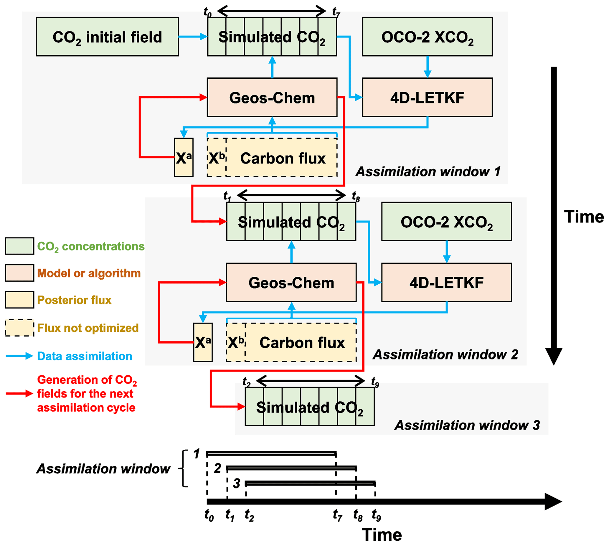
We developed a Bayesian atmospheric inversion system (Fig. 1) to infer daily gridded surface carbon fluxes (excluding fossil fuel and biomass burning emissions, which were prescribed) from OCO-2 XCO2 retrievals. This system was built upon the GEOS-Chem global transport model coupled with the 4D-LETKF algorithm (Hunt et al., 2007) and is analogous to identifying a weight that linearly combines the ensemble members of carbon fluxes to obtain best-fitting CO2 observations. Our system assimilates OCO-2 XCO2 on an ongoing basis and optimizes carbon fluxes on the first day of each data-assimilation window for each grid cell independently by minimizing a cost function as follows (Eq. 1):
where x is a control vector consisting of variables to be optimized (i.e., the scale factors of the surface fluxes in each grid cell), xb is a prior guess corresponding to the control vector x with errors represented by a covariance matrix B, y is an observation vector that gathers the OCO-2 XCO2 retrievals, R represents the error covariance matrix, and H is the observation operator, which calculates the OCO-2-equivalent XCO2 value from the GEOS-Chem simulations, OCO-2 XCO2 prior, and column-averaging kernel. The cost function J(x) measures the differential surface carbon fluxes between the prior (xb) and optimized (x) estimates plus the difference in the XCO2 fields between the OCO-2 observations (y) and GEOS-Chem simulations (H(x)); these two terms are weighted using the prior errors (B) and observation errors (R), respectively.
In each data-assimilation window, the control vector (x) is optimized through Eqs. (2)–(5) as follows (Hunt et al., 2007):
where a and b represent the posterior and prior state, respectively, k represents the ensemble size (i.e., 24), is the ensemble mean of the control vector, X is the ensemble perturbation matrix whose ith column represents , yo contains the assimilated OCO-2 XCO2 within the data-assimilation window and localization length, is the mean of a prior XCO2 field averaged over simulations, Yb is the ensemble perturbation matrix whose ith column represents , is a weight vector, is the analysis covariance matrix, and I is the identity matrix.
The ensemble mean is calculated by obtaining the average optimized result from the 2 previous time steps and a fixed value of 1 (Peters et al., 2007), thus propagating the optimized information from 2 previous time steps to the current state and representing a moving average smoothing technique that suppresses variations in xb over time. The prior covariance matrix B was constructed based on a normal distribution with the standard deviation of 3.0 within a spatial correlation length of 2000 km, and the spatial correlation of the prior flux errors between ocean and land is set to zero in our inversion. The ensemble perturbation matrix Xb was constructed through Cholesky decomposition to B (i.e., , and the ensemble members were generated by adding the ensemble mean to the ith column of Xb. The term is a weight vector that specifies the linear combinations of ensemble perturbations Xb that are added to the prior mean to estimate the posterior mean . The ensemble mean of is then used to update the carbon fluxes on the current day, thus driving another GEOS-Chem simulation to generate the initial CO2 concentration fields for the next data-assimilation cycle.
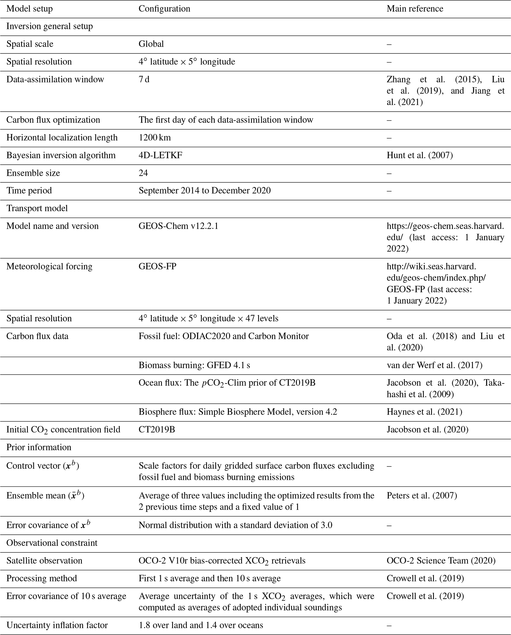
Our inversion system configuration is summarized in Table 1. The data-assimilation window was set to 7 d based on the inversion system configurations of Zhang et al. (2015), Liu et al. (2019), and Jiang et al. (2021). In each data-assimilation cycle, the ensemble members xb(i) (with the ensemble mean and perturbations Xb to approximate B) are initialized on the first day of the data-assimilation window, and the following 6 d use the same without perturbation. The carbon fluxes representing the first day of each window are optimized based on the link between the modeled XCO2 and observed XCO2 within the data-assimilation window. The GEOS-Chem model and prior fluxes are described in Sect. 2.2 below, and Sect. 2.3 describes how the OCO-2 XCO2 observations and their uncertainties were assimilated. In Sect. 2.4, we designed four sensitivity inversions to vary the prior fluxes and prior uncertainty statistics and investigate their influence on the inversion results. The procedure followed to evaluate the posterior fluxes and independent observations are presented in Sect. 2.5.
Table 1Configuration of the atmospheric carbon inversion system developed in this study.
2.2 Transport model and carbon fluxes
The GEOS-Chem is a global 3D chemical transport model (Bey et al., 2001; https://geos-chem.seas.harvard.edu/, last access: 1 January 2022) driven by meteorological fields obtained from the Goddard Earth Observing System (GEOS) of the National Aeronautics and Space Administration (NASA) Global Modeling and Assimilation Office. The GEOS-Chem model has been applied to develop global carbon inversion systems by several research groups worldwide (Feng et al., 2009; Deng et al., 2014; and Liu et al., 2021), and the resulting systems vary according to their model versions, data-assimilation methods, and utilized prior fluxes. Here, we used GEOS-Chem v12.2.1 in our inversion system to simulate the global CO2 transport and relate surface carbon fluxes to observed atmospheric CO2 gradients at a horizontal resolution of 4∘ latitude ×5∘ longitude, driven by GEOS-FP meteorology data. Such a spatial resolution is sufficient to capture large-scale atmospheric CO2 transport along with the associated spatiotemporal variability and can achieve a balance between ensemble simulations and computational costs.
We distinguished among four CO2 flux categories in the GEOS-Chem model, including fossil fuel fluxes, biomass burning fluxes, ocean fluxes, and terrestrial biospheric fluxes. The fossil fuel emissions from land and international bunker sources were derived from the Open-source Data Inventory for Anthropogenic CO2 (ODIAC, version 2020) dataset (Oda et al., 2018) for 2014–2019, and we downscaled the dataset from the monthly to hourly scale based on temporal scaling factors obtained from the Temporal Improvements for Modeling Emissions by Scaling (TIMES) database (Nassar et al., 2013). The 2020 emissions were estimated by extrapolating daily 2019 emissions based on the emission growth rates from 2019 to 2020 derived from the Carbon Monitor project (Liu et al., 2020, https://carbonmonitor.org/, last access: 1 January 2022). The biomass burning emissions were obtained from the Global Fire Emissions Database (GFED) 4.1s (van der Werf et al., 2017) from 2014 to 2020; this database provides monthly emissions of different fire types and daily and 3-hourly temporal profiles. These monthly biomass burning emissions were downscaled to 3-hourly fluxes. Ocean–atmosphere CO2 fluxes on a 3-hourly basis were obtained from the pCO2-Clim prior of the CarbonTracker version CT2019B (Takahashi et al., 2009; Jacobson et al., 2020). The 3-hourly terrestrial biospheric fluxes were derived from the Simple Biosphere Model, version 4.2 (SiB4) global hourly dataset (Haynes et al., 2021). We halved the gridded terrestrial biospheric fluxes to dampen the seasonal cycle and then integrated annual fluxes as zero over land based on the balance between gross primary production and respiration in the SiB4 model, thus implying that the spatiotemporal variabilities in inferred terrestrial fluxes from our inversion system were mainly determined by the assimilated observations. The 2018 prior ocean and terrestrial biospheric fluxes were used for the 2019 and 2020 inversions because CT2019B and SiB4 data were available up to 2018 at present.
2.3 Assimilated OCO-2 observations
The OCO-2 is the first dedicated CO2-monitoring satellite designed by NASA; this satellite was launched in July 2014 (Eldering et al., 2017). It flies in a sun-synchronous, near-polar orbit 705 km above the Earth's surface with a repeat cycle of 16 d and a local overpass time of approximately 01:30 pm. The OCO-2 satellite collects 8 adjacent cross-track samples every 0.333 s (24 samples per second) at a spatial resolution of 1.29 km × 2.25 km for each footprint at nadir. We assimilated the OCO-2 Level 2 bias-corrected XCO2 retrievals, retrospective processing V10r (OCO-2 Science Team, 2020) in our inversion system. Figure 2 presents the spatial and seasonal distributions of valid OCO-2 V10r XCO2 retrievals over the 4∘ × 5∘ GEOS-Chem grid cells between 2015 and 2020.
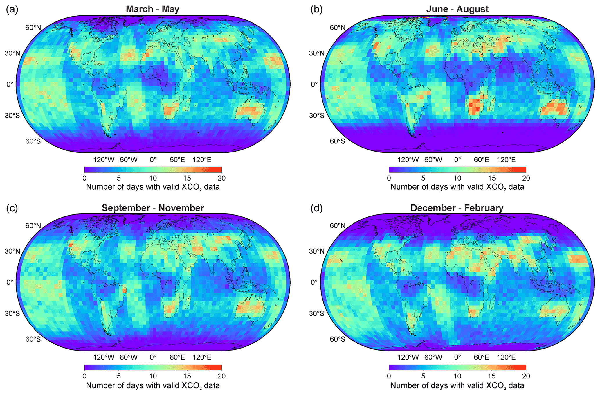
Figure 2Spatial and seasonal distributions of the valid OCO-2 XCO2 retrievals between 2015 and 2020. The numbers of days with valid OCO-2 XCO2 retrievals (xco2_quality_flag = 0) in each GEOS-Chem 4∘ × 5∘ grid cell are shown for the periods spanning (a) March–May, (b) June–August, (c) September–November, and (d), and December–February. The values shown here represent annual averages between 2015 and 2020.
The high-density OCO-2 XCO2 retrievals were preprocessed to generate 1 and 10 s averages before being assimilated because the retrieval errors were closely correlated both temporally and spatially (Crowell et al., 2019). First, the “good” retrievals in the OCO-2 Lite files were selected according to the “xco2_quality_flag” variable and filtered to remove outliers in each orbit using the “3 times the standard deviation” rule, i.e., XCO2 values whose differences from their adjacent soundings deviated from the mean by more than 3 times the standard deviation were filtered out and not used in the subsequent data-assimilation process. Then, the 1 and 10 s averages and their uncertainties are computed using the formulas from Crowell et al. (2019). The 1 s averages were computed from the selected good retrievals across each 1 s span along the OCO-2 tracks using the method described by Crowell et al. (2019). The inverse error variance obtained for each XCO2 retrieval was used to calculate a weighted average for all related variables with the uncertainty represented by an average uncertainty of the adopted single soundings. Finally, 10 s averages were computed across each 10 s span (approximately corresponding to a ground track 70 km in length) by weighting the 1 s averages by their inverse variance values. The uncertainty of these 10 s averages was estimated as an average uncertainty for the adopted 1 s averages and was inflated by factors of 1.8 and 1.4 over land and oceans, respectively; the results thus accounted for the representation errors that arose due to the mismatches between the GEOS-Chem model and assimilated OCO-2 observation resolutions. The 10 s averages were then assimilated to our inversion system while assuming independence among the different 10 s spans.
2.4 Sensitivity inversion experiments
We performed four inversion sensitivity experiments using different prior fluxes, uncertainty configurations, and data-assimilation window lengths to investigate the influence of these factors on the resulting carbon inversions (Table 2). Based on the reference inversion, we reduced and increased the standard deviations of the normal distributions used to represent the error structures of xb in sensitivity experiments no. 1 (S_exp1) and no. 2 (S_exp2), respectively, to quantify the influence of the ensemble spread of xb on the carbon inversion results. In sensitivity experiment no. 3 (S_exp3), the prior terrestrial biospheric fluxes from CT2019B were used; these fluxes are based on the Carnegie-Ames-Stanford Approach (CASA) biogeochemical model, and the other configurations remained the same as those used in the reference inversion. The comparison between S_exp3 and our reference inversion illustrates the impact of different prior terrestrial biospheric fluxes on the inversion results. In sensitivity experiment no. 4 (S_exp4), the data-assimilation window length was doubled to 14 d compared to the reference inversion, which tends to constrain fluxes based on more OCO-2 observations in each data-assimilation window. All four sensitivity inversions were performed considering the period from September 2014 to December 2015, thus providing inversion results in 2015 for use and comparison in our analysis.
Table 2Sensitivity inversion experiments conducted in this study.

2.5 Evaluation of posterior fluxes
We compared the GEOS-Chem-modeled dry-air mole fractions of CO2 based on posterior fluxes with independent surface and aircraft measurements to evaluate the posterior fluxes. These measurement data were not assimilated into our inversion system. Such evaluation methods have been widely used to evaluate global carbon budget estimates inferred from atmospheric inversion (Chevallier et al., 2019; Crowell et al., 2019). The evaluation observation datasets were obtained from the CO2 GLOBALVIEWplus v7.0 ObsPack database (Cooperative Global Atmospheric Data Integration Project, 2021), which is maintained by the Earth System Research Laboratory (ESRL) of the National Oceanic and Atmospheric Administration (NOAA) (https://www.esrl.noaa.gov/gmd/ccgg/obspack/, last access: 1 January 2022). The ObsPack framework (Masarie et al., 2014) archives direct atmospheric greenhouse gas measurements from different laboratories to support carbon cycle modeling research. We collected flask sample measurements from 52 stations (Table S1) at altitudes lower than 3000 m and aircraft measurements from 3 programs (i.e., ABOVE, ACT, and TOM, please see Table S2) between 2015 and 2020. To perform the evaluation, GEOS-Chem model-simulated CO2 concentrations were sampled at the locations and times corresponding to the observation data points to calculate the multiannual mean bias and root mean square error (RMSE) values by season and by latitude band.
In addition, we collected surface carbon flux estimates from different atmospheric inversion models, including NOAA's CT2019B (Jacobson et al., 2020), the Copernicus Atmosphere Monitoring Service (CAMS) model versions v20r2 and v20r3 (Chevallier et al., 2005), Jena CarboScope version sEXTocNEET_v2021 (Rödenbeck et al., 2018), and the Carbon Monitoring System Flux (CMS-Flux) (Liu et al., 2021). These carbon budget products were built upon different atmospheric inversion frameworks that vary with different transport models, observation constraints, and data-assimilation techniques. We performed comprehensive comparisons at both the global and regional scales to evaluate our inversion estimates.
3.1 Global carbon budget
The annual global carbon budgets derived using our inversion system are shown for 2015–2020 in Table 3. The mean annual terrestrial flux, i.e., the sum of the net ecosystem exchange (NEE) (− 3.91 GtC yr−1) and fire (1.88 GtC yr−1) fluxes, was estimated as − 2.02 GtC yr−1, and the mean annual oceanic flux was estimated as − 2.34 GtC yr−1. On average, the terrestrial and oceanic fluxes compensated for 21 % and 24 %, respectively, of the global fossil CO2 emissions (9.80 GtC yr−1), with the remaining 55 % of fossil CO2 emissions (5.44 GtC yr−1) remaining in the atmosphere. Our inversion results agreed with NOAA's surface measurement-based atmospheric CO2 growth rates (https://gml.noaa.gov/ccgg/trends/gl_gr.html, last access: 1 January 2022); this source reported average annual growth of 5.39 GtC yr−1 from 2015 to 2020 based on the conversion factor of 2.124 GtC ppm−1 (Friedlingstein et al., 2022). The derived bias of 0.05 GtC yr−1 was slightly lower than the bias range of the atmospheric inversion models (0.06–0.17 GtC yr−1) that participated in the Global Carbon Budget 2021 (GCB2021) project (Friedlingstein et al., 2022). The broad consistency between our inversion results and the atmospheric CO2 growth rate from measurement suggests that the net atmosphere–surface exchange of CO2 was well constrained by our inversion system.
Table 3Global anthropogenic CO2 budget from 2015–2020 derived from our reference inversion results and NOAA's atmospheric CO2 growth rate. All values are in GtC yr−1.

a NEE represents the net ecosystem exchange. b Net flux represents the sum of the NEE and fire fluxes. c NOAA's CO2 growth rates were obtained from https://gml.noaa.gov/ccgg/trends/gl_gr.html (last access: 1 January 2022) and were estimated based on the conversion factor of 2.124 GtC ppm−1 (Friedlingstein et al., 2022). d Annual average estimates between 2015 and 2020.
The global carbon budget partitioning results are shown in Fig. 3, including our reference inversion results, other state-of-the-art atmospheric inversion estimates, and the ensemble estimates from GCB2021 (riverine flux-adjusted) for 2015–2018, i.e., the common period when all of these data were available. The integrated land (with fossil CO2 emissions) and ocean fluxes were scattered around the diagonal purple line denoting the atmospheric growth rate in Fig. 3a, suggesting that the global-scale CO2 fluxes were conserved and well-constrained in all of the considered inversion models, although these models assimilated different CO2 observations using various strategies. Our inversion system used a relatively large prior for land fluxes involving a combination of prescribed biomass burning emissions (∼1.80 GtC yr−1) and annually zero terrestrial biospheric fluxes, while the other inversion models used annually zero or negative prior natural land fluxes (Fig. 3b). Despite the large prior land fluxes used by our model (denoted by the open red circles shown in Fig. 3a and b), our inversion system successfully corrected the global fluxes to match the atmospheric CO2 growth rates (the solid red circles in Fig. 3a and b). The major discrepancies derived from different inverse models involved the partitioning scheme between land and ocean fluxes. Our inversion results, as well as CAMS and Jena, estimated smaller land fluxes and ocean uptakes than CMS-Flux and CT2019B. The GCB2021 estimates are comparable to our inversion estimates but present a large budget imbalance (− 0.63 GtC yr−1 averaged between 2015 and 2018) due to model deficiencies (Friedlingstein et al., 2022); this imbalance explained why the purple circles representing the GCB2021 estimates were not located on the purple lines in Fig. 3a and b.
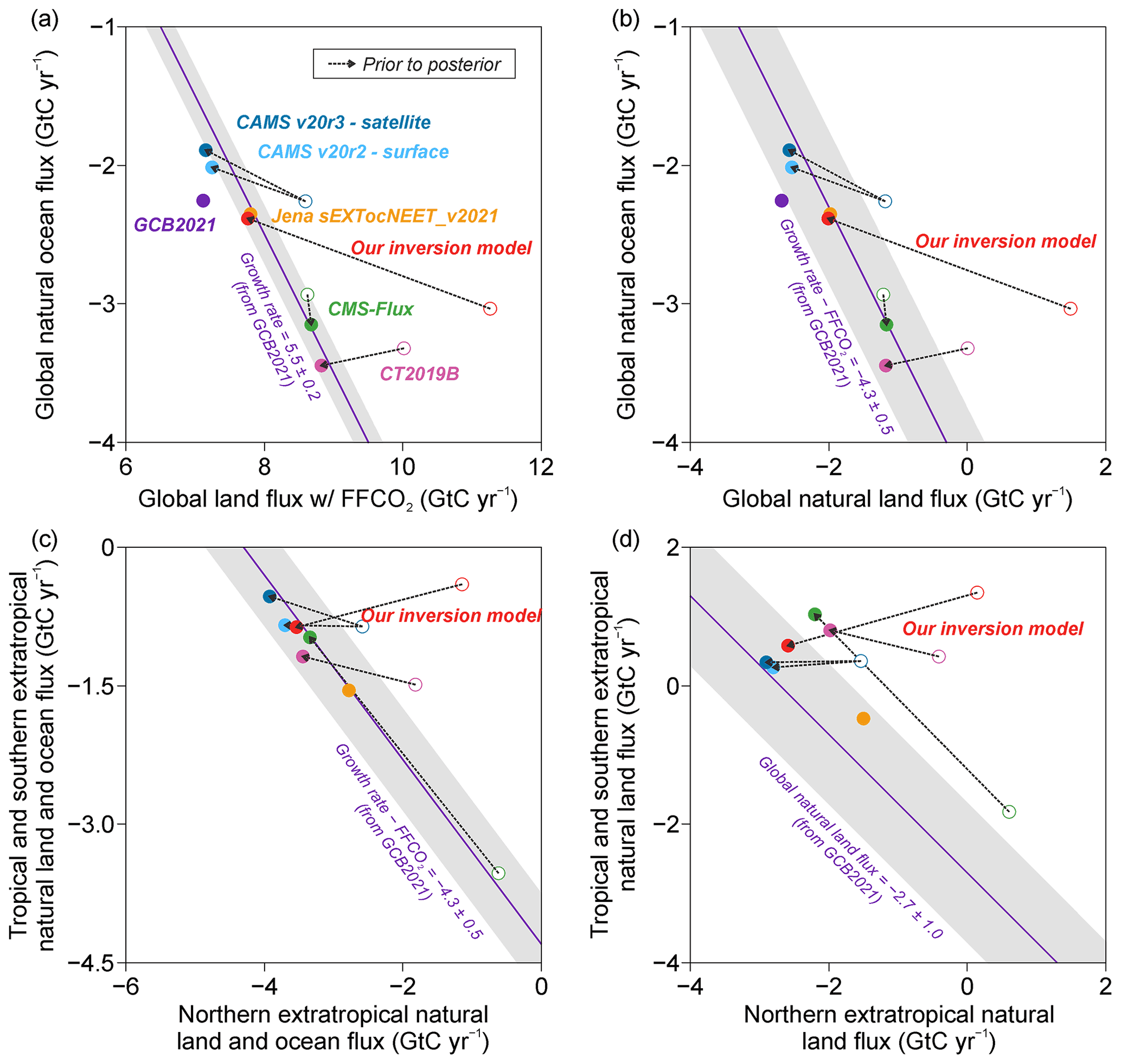
Figure 3Global carbon flux partitioning schemes between the land and ocean and among different latitudinal bands for 2015–2018. The atmospheric inversion results are represented by solid circles (representing posterior fluxes) and open circles (representing prior fluxes (if any)). The red circles represent the carbon flux estimates derived from our reference inversion results; the blue circles represent the results of the CAMS versions v20r2 and v20r3 (Chevallier, et al., 2005); the orange circles represent the Jena CarboScope version sEXTocNEET_v2021 results (Rödenbeck et al., 2018); the green circles represent the CMS-Flux results (Liu et al., 2021); and the pink circles represent the results of the NOAA CarbonTracker version CT2019B (Jacobson et al., 2020). The purple circles in panels (a) and (b) represent the GCB2021-derived (riverine flux-adjusted) estimates (Friedlingstein et al., 2022). The purple line and equation in each panel represent the sum of the x and y variables derived from GCB2021, and the gray shaded area represents the error equivalent to 1 standard deviation. The purple lines thus have a slope of −1, and any deviation perpendicular to these purple lines indicates disagreements in the GCB2021 estimates, including the purple circles in panels (a) and (b) derived from the GCB2021 results due to carbon budget imbalances.
The differences among inversion-based global carbon budget estimates are mainly attributed to the natural components, not fossil fuel emissions, as illustrated by the large spread of natural fluxes (without the prescribed fossil CO2 emissions) in Fig. 3b. This finding differs from previous intercomparison studies in which global atmospheric CO2 inverse models were shown to disagree on fossil fuel priors (Gaubert et al., 2019). All of the atmospheric inversion models shown in Fig. 3 adopted consistent fossil CO2 priors with an annual average of 9.7–10.0 GtC yr−1 from 2015 to 2018, benefiting from the community efforts to constrain uncertainties associated with fossil fuel emissions and converge on global total carbon sinks. However, the land–ocean partitioning schemes of natural fluxes are much more uncertain and can reflect spreads up to 1.6 GtC yr−1 (Fig. 3b), comparable with the uncertainties associated with the land–ocean partitioning scheme due to transport model differences reported by Basu et al. (2018). Moreover, we found that the global oceanic fluxes seemed to be largely unchanged relative to the ocean priors used in different inverse models (Fig. 3b), likely due to the weak observational constraints over oceans. The usage of prior ocean fluxes that differ by 1.1 GtC yr−1 among inverse models thus plays an important role in determining the land–ocean partitioning schemes of global fluxes in atmospheric inversion results.
3.2 Regional carbon budget
3.2.1 Latitudinal distribution of fluxes
The partitioning divides between the northern extratropics (23–90∘ N) (NET) and the tropics (23∘ S–23∘ N) (T) + southern extratropics (90–23∘ S) (SET) are illustrated in Fig. 3c and d. The integrated fluxes from NET and T + SET are anticorrelated and scattered around the global atmospheric growth rate of CO2 minus the fossil CO2 emissions listed in GCB2021 (the diagonal purple line in Fig. 3c), suggesting that the global total natural fluxes were well-constrained by atmospheric inversion. Our inversion results suggest that NET and T + SET represent average natural fluxes of − 3.5 and − 0.9 GtC yr−1, respectively, between 2015 and 2018, both of which lie within the ensemble of different inversion model estimates (Fig. 3c and d). Land fluxes dominate over ocean fluxes in NET, which are estimated as − 2.6 and −0.9 GtC yr−1, respectively, on average between 2015 and 2018. However, in T + SET, ocean fluxes (−1.4 GtC yr−1) dominate over land fluxes (0.6 GtC yr−1), because the area of ocean is much larger than land in this region. The differences among inversion model estimates could be attributed to land–ocean partitioning by latitude, although the discrepancies in posterior fluxes derived are largely reduced compared to the prior fluxes after assimilating the OCO-2 CO2 observations. The GCB2021 results tended to give larger land sinks than all of the atmospheric inversion models except for CAMS (Fig. 3d), although the large budget imbalance of GCB2021 complicated the interpretation of these large flux discrepancies. The disagreements among multiple inversion models over latitude indicated the existence of substantial uncertainties in the regional carbon budget estimates.
3.2.2 Regional distribution of fluxes
Figure 4 presents the spatial distribution of the natural fluxes derived from our reference inversion model, including both prior and posterior annual average fluxes between 2015 and 2020. We estimated a net land carbon flux of −2.4 GtC yr−1 between 2015 and 2020 over the Northern Hemisphere; this value was slightly larger than the GtC yr−1 estimate obtained from 2000 to 2010 by Ciais et al. (2019) based on a two-box atmospheric inversion model. Figure 4 shows that large carbon sinks are located in the northern forests and woodlands over the eastern USA, Asia, and Europe, as well as in the tropical evergreen forests over South America and Africa (Fig. 4c). Since the prior biospheric annual flux was integrated as zero over land globally (Fig. 4a), the spatial distribution of the posterior carbon sinks was reconstructed only by the assimilated OCO-2 XCO2 through atmospheric inversion. When the biomass burning fluxes were added, as was prescribed in our inversion system (Fig. 4b), we observed large flux gradients over South America, southern Africa, and the Eurasia boreal region in the posterior fluxes (Fig. 4d) due to extensive savanna and forest fires (van der Werf et al., 2017).
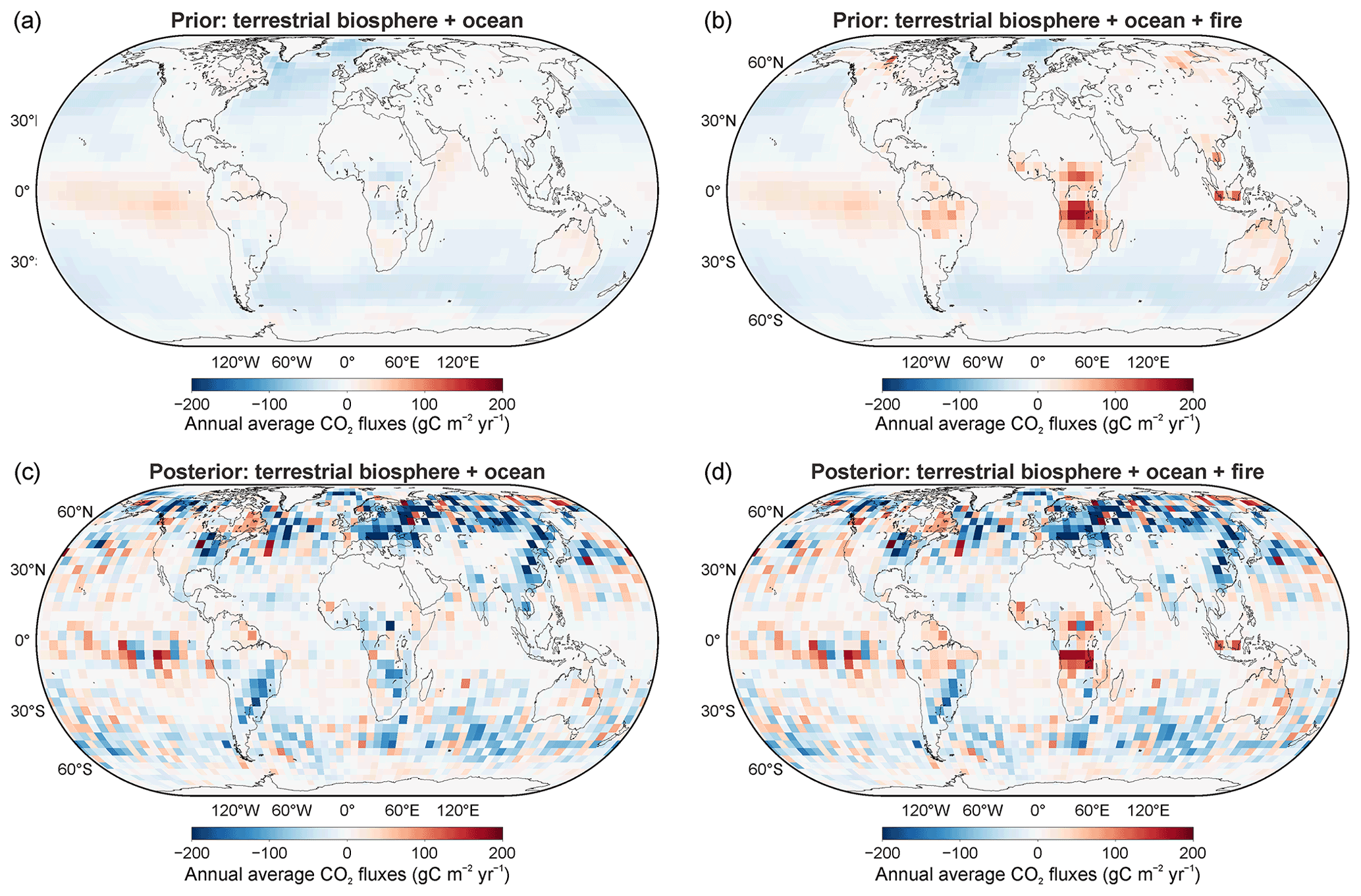
Figure 4Spatial distribution of global natural carbon fluxes from 2015 to 2020. The annual average carbon fluxes derived from 2015 to 2020 are shown at a spatial resolution of 4∘ latitude × 5∘ longitude. Panel (a) displays the prior terrestrial biospheric + oceanic fluxes used in the reference inversion system. Panel (b) shows the prior terrestrial biospheric + oceanic + fire fluxes (the fire fluxes were prescribed in the inversion system). Panel (c) shows the posterior terrestrial biospheric + oceanic fluxes derived from the reference inversion system. Panel (d) shows the posterior terrestrial biospheric + oceanic + fire fluxes.
Over the 11 TransCom land regions (Fig. 5), our inversion results were broadly consistent with the other atmospheric inversion products, although we did observe an unsurprising lack of agreement due to large uncertainties in regional flux estimates. Northern Africa, southern Africa, and South American tropical regions all represent net carbon sources due to the substantial fire emissions, especially from forest fires, in these regions. Large net carbon uptakes occur over North America, Eurasia, and Europe, where our inversion model estimated annual average fluxes of − 0.3, − 1.4, and − 0.9 GtC yr−1, respectively. Further, these estimates broadly agreed with the ensemble of surface observation-based atmospheric CO2 inversions derived between 2001 and 2004 (Peylin et al., 2013), which provided flux values of , , and GtC yr−1, respectively, over these three regions. Our inversion model seemed to estimate slightly lower fluxes over the boreal and temperate regions in North America than the other inversion models. The OCO-2 land observations were limited to lower latitudes during fall and winter in the Northern Hemisphere (Fig. 2), and the retrieval biases increased with the solar and satellite zenith angles (O'Dell et al., 2018). We would therefore speculate that the sampling and retrieval biases of the OCO-2 satellite at high latitudes weakened the capability of our inversion system to constrain land fluxes over boreal regions. Since total net natural fluxes are conserved globally, flux overestimations of similar magnitudes in other regions typically compensate for flux underestimations in particular regions through the atmospheric inversion process, thus resulting in large variations in regional flux estimates among different inversion models.
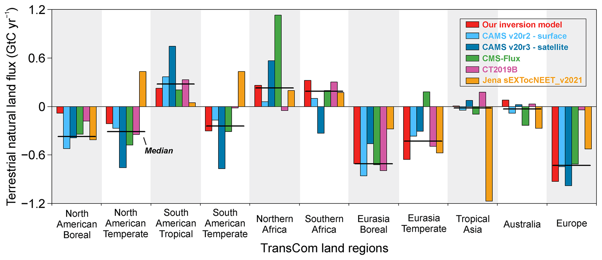
Figure 5Terrestrial natural land fluxes derived over the 11 TransCom land regions from 2015 to 2018. Each atmospheric inversion is represented by bars showing the posterior natural land flux (i.e., terrestrial biospheric + fire fluxes) averaged between 2015 and 2018 in each TransCom land region; the black lines represent the median values of all six inversion estimates. The colors of the atmospheric inversion models are the same as those shown in Fig. 3, and the references for each inversion model are included in the caption of Fig. 3.

Figure 6Seasonal cycle amplitudes of natural land fluxes over different latitudinal bands from 2015 to 2018. The global natural land fluxes (i.e., terrestrial biospheric + fire fluxes) averaged between 2015 and 2018 were split into four zonal bands: (a) northern high latitudes (50–90∘ N), (b) northern mid-latitudes (23–50∘ N), (c) tropics (23∘ S–23∘ N), and (d) southern extratropics (90–23∘ S). Each atmospheric inversion result was represented by solid curves (posterior flux) and dashed circles (prior flux (if any)). The colors of the atmospheric inversion models are the same as those shown in Fig. 3, and the references for each inversion model are listed in the caption of Fig. 3.
3.3 Seasonal cycle of carbon fluxes
The different atmospheric inversion systems analyzed herein presented broadly consistent phases (source-to-sink transitions) and amplitudes (peak-to-trough differences) of the seasonal natural land flux cycle, except over the tropical region (23∘ S–23∘ N) (Fig. 6). Predominant sinks were identified over the Northern Hemisphere during the growing season, with maximum monthly sinks occurring in July (Fig. 6a and b). The prior flux used in our inversion system revealed a smaller carbon uptake in July (the dashed red curves in Fig. 6a and b); this peak is substantially enlarged (the solid red curves in Fig. 6a and b) in the posterior fluxes after assimilating OCO-2 XCO2. During fall and winter in the Northern Hemisphere, the shift from sink to source is consistently reproduced by different atmospheric inversion models, although the satellite-based posterior fluxes tend to follow the pattern of the prior due to a lack of valid OCO-2 XCO2 retrievals over the 50–90∘ N region (Fig. 2c and d). Overall, satellite-based inversions (e.g., our inversion model, CAMS v20r3, and CMS-Flux) tended to differ from the surface-based inversions (e.g., CAMS v20r2, CT2019B, and Jena) regarding the output peak sink estimates in the growing season. The satellite-based inversions estimated carbon fluxes of − 1.28 to − 1.38 GtC month−1 over 50–90∘ N in July (Fig. 6a), and these values were slightly smaller than the surface-based inversion estimates (− 1.58 to − 1.83 GtC month−1). Over the 23–50∘ N latitudinal band (Fig. 6b), the satellite-based inversions estimated larger carbon uptake magnitudes (− 0.94 to − 1.19 GtC month−1) in July than the surface-based inversions did (− 0.82 to − 0.98 GtC month−1).
The peaks and troughs identified in the carbon fluxes over the tropics (23∘ S–23∘ N) were not consistently represented by different atmospheric inversion models (Fig. 6c), indicating the need for collective efforts to improve tropical carbon budget estimates. A small seasonal cycle amplitude was revealed by our inversion results, CT2019B, and Jena, while the CMS-Flux and the two CAMS inversion models all presented relatively large seasonal cycle amplitudes. These substantial discrepancies could potentially be attributed to a lack of strong CO2 observational constraints and the difficulty of accurately simulating atmospheric transport processes in the tropics. The OCO-2 satellite is expected to provide broad coverage but is greatly hindered by cloud coverage during the wet season and aerosol pollution from biomass burning during the dry season in the tropics. In addition, in previous satellite-based inversions, researchers preferred not to use OCO-2 ocean glint observations due to known uncertainty issues (O'Dell et al., 2018), which substantially reduced the number of assimilated OCO-2 observations over the tropics. The OCO-2 V10r satellite retrievals are thought to have improved these ocean glint observations, which were used as observational constraints in our inversion system. Over the mid- to high latitudes of the southern atmosphere (90–23∘ S), where much less land is present, the natural land flux inversion estimates did not depart largely from the priors and were highly consistent among different inversion models (Fig. 6d).
Over the 11 TransCom regions, our inversion results exhibited seasonal cycle amplitudes similar to those of the other analyzed inversion models (Fig. 7). The peak summertime drawdown of fluxes in the northern ecosystems, which represents the deeper sinks during the growing season, is consistently constrained by different inversion systems over the North American boreal (Fig. 7a), North American temperate (Fig. 7b), Eurasian boreal (Fig. 7g), Eurasia temperate (Fig. 7h), and European (Fig. 7k) regions. However, these regions reveal relatively large ensemble spreads in their carbon source estimates during fall and winter due to the sparse satellite observational constraints and divergent seasonal amplitudes of the prior fluxes used in the inversion process, which finally result in large discrepancies in the annual flux estimates. For example, our inversions exhibited relatively small annual fluxes over the North American boreal region compared to the other inversion estimates (Fig. 5), and this was mainly due to the larger carbon sources derived between September and February (Fig. 7a). We also observed substantial disagreements in the seasonal cycle of the flux amplitude over the South American tropical (Fig. 7c), tropical Asia (Fig. 7i), and Australian (Fig. 7j) regions; these amplitudes were found to be close to carbon neutral based on the ensemble of different inversion models (Fig. 5) but diverged widely with regard to their annual and monthly flux estimates.

Figure 7Seasonal cycle amplitudes of the natural land fluxes derived over the 11 TransCom land regions from 2015 to 2018. Each atmospheric inversion is represented by a solid curve representing the posterior natural land flux (i.e., terrestrial biospheric + fire fluxes) averaged between 2015 and 2018; the colors are the same as those shown in Fig. 3. The references for each inversion model are listed in the caption of Fig. 3.
3.4 Evaluation with CO2 measurements
The GEOS-Chem-modeled XCO2 outputs based on posterior fluxes matched the OCO-2 XCO2 retrievals in terms of both their magnitudes (Fig. S1) and trends (Fig. S2), thus suggesting that our inversion system was effectively constrained by the assimilated OCO-2 XCO2 values. The modeled RMSEs of the posterior fluxes against the OCO-2 XCO2 values were constrained by our inversion system (Fig. S1). The posterior simulations (the red curves in Fig. S2) corrected the overestimated prior-modeled XCO2 values (the blue curves in Fig. S2) compared to the OCO-2 observations (black curves in Fig. S2) by adding terrestrial carbon uptake to the prior flux. Regarding the trends and interannual variability, the simulations driven by prior fluxes overestimated the increasing XCO2 over the Northern and Southern hemispheres, and this was corrected in our inversion system by increasing the terrestrial carbon sinks from 2015 to 2020 (Table 3).
The atmospheric CO2 concentration measurements obtained at surface (Table S1) and by aircraft (Table S2) networks both confirmed that the CO2 values modeled based on posterior fluxes (the red curves in Fig. 8) were improved relative to those based on prior fluxes (the blue curves in Fig. 8); thus, this process substantially reduced the biases (Fig. 8a–c) and RMSEs (Fig. 8d–f) compared to the CO2 observations with regards to both latitude and altitude. The daily, seasonal, and interannual variations in surface CO2 concentrations were reproduced in the posterior flux-based simulations, as illustrated by the six selected stations (Fig. S3) that varied by latitude and altitude and provided continuous measurement records between 2015 and 2020. The comparisons with aircraft observations in the free troposphere (above 3000 m) showed slightly smaller biases (Fig. S4) because these measurements were less affected by local sources (Chevallier et al., 2019). The evaluations conducted at the three atmospheric layers all presented large RMSEs in NET (Fig. 8), suggesting that the inversion estimates of CO2 fluxes in this region tended to have relatively larger uncertainties than the other latitudes; this finding was consistent with the atmospheric inversion ensemble assessment of Crowell et al. (2019). The NET are dominated by land but lack adequate, high-quality OCO-2 XCO2 retrievals during fall and winter, therefore contributing weak observational constraints to the flux outputs.
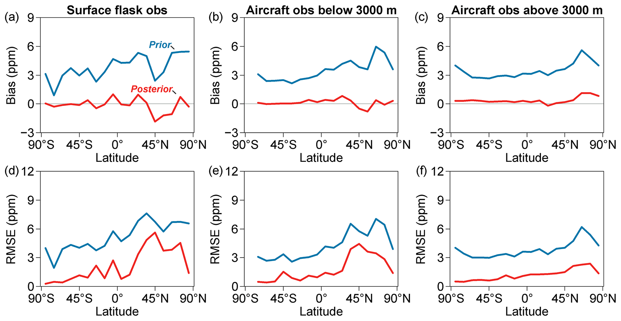
Figure 8Comparisons of GEOS-Chem-modeled dry-air mole fractions of CO2 with surface and aircraft measurements. The simulations driven by the prior (blue curves) and posterior (red curves) fluxes of our reference inversions between 2015 and 2020 were evaluated against surface flask observations (a, d), aircraft observations obtained below 3000 m a.s.l. (b, e), and aircraft observations obtained above 3000 m (c, f) to derive the model biases (a–c) and RMSEs (d–f). The surface and aircraft measurement programs are summarized in Tables S1 and S2, respectively.
4.1 Influence of prior fluxes and uncertainties
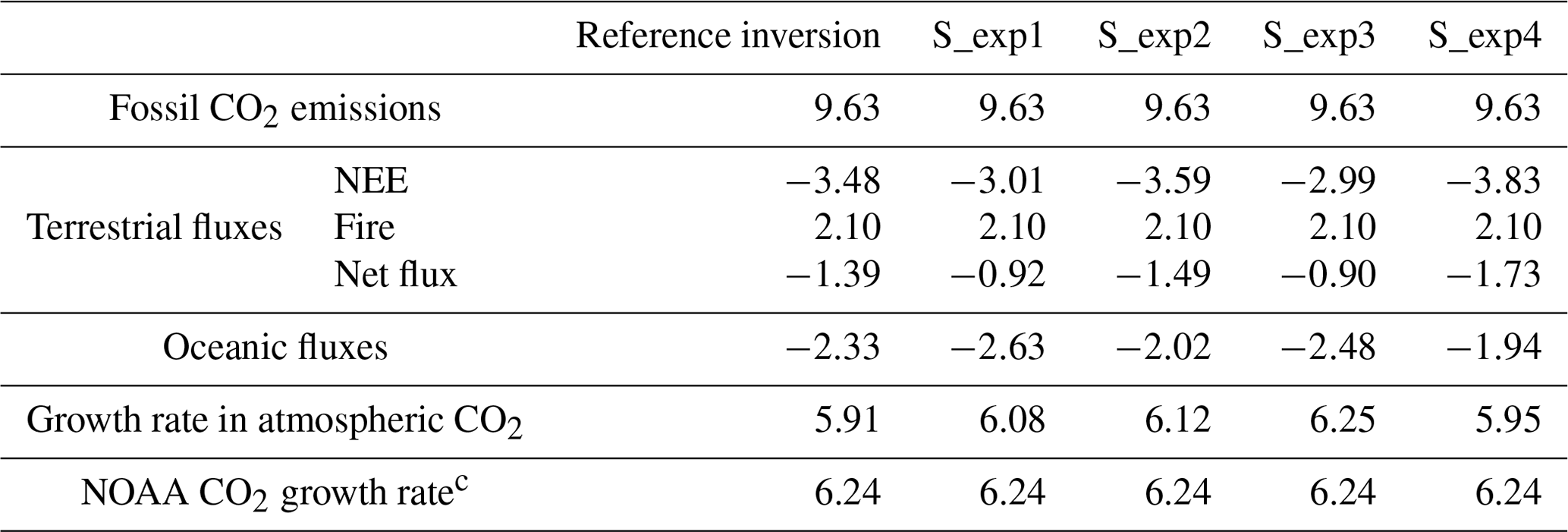
The sensitivity inversion results diverged with regard to the land and oceanic fluxes (Table 4), although all inversion results agreed with the NOAA's atmospheric CO2 growth rates, suggesting that the prior fluxes associated with uncertainties altered the global carbon budget partitioning scheme in the atmospheric inversion results. The global NEE derived from our reference inversion model was − 3.48 GtC yr−1 in 2015; this value was substantially different from the S_exp1–S_exp4 estimates (− 2.99 to −3.83 GtC yr−1). The global oceanic flux inversion estimates were adjusted accordingly in each inversion to match the atmospheric CO2 growth rates. Based on the evaluations performed using surface CO2 measurements (Fig. S5), our reference inversion results presented slightly smaller biases and RMSEs in the modeled CO2 over the tropics and northern latitudes than S_exp1, S_exp2, and S_exp4. The prior fluxes used in S_exp3 were derived from the CASA model (Table 2), and this experiment exhibited better performances in the northern mid-latitudes but presented larger biases and RMSEs than the reference inversion in the northern high latitudes, possibly due to weaker constraints associated with satellite observations and inappropriate prior fluxes used in this region. Increasing the data-assimilation window length to 14 d (S_exp4) slightly increased the global NEE and decreased the oceanic fluxes (Table 4), while the inversion model performance evaluated with surface measurement of CO2 concentrations are not improved (Fig. S5).
Table 4Global anthropogenic CO2 budget for 2015 derived from our reference inversion results and four sensitivity inversion experiments. All values shown here represent the global total fluxes for 2015 in GtC yr−1.
The TransCom land regions showed different sensitivities to the prior fluxes used in the atmospheric inversion process at the annual (Fig. 9) and monthly (Fig. 10) timescales. For example, the flux estimates were broadly consistent among different inversion experiments over the Eurasia temperate region and Europe, where the inversions were not as sensitive as other regions to prior information due to the stronger observational constraints of the OCO-2 satellite measurements over mid-latitudinal areas. The sensitivity inversion estimates of fluxes are also broadly consistent over southern Africa, the Eurasia boreal region, and Australia. In contrast, the flux estimates over the North American boreal and North American temperate regions differed greatly in their signs and magnitudes across sensitivity inversions because the atmospheric inversion system not only gave more weight to the prior information but also represented the residual fluxes resulting from global optimization over these regions due to the weak observational constraints available in fall and winter (Fig. 10a and b). Large differences were also evident over the tropics (e.g., the South American tropical region, northern Africa, and tropical Asia) due to cloud- and aerosol-caused gaps in the satellite observations. In S_exp3, the amplitude in the seasonal cycle of carbon fluxes in the South American tropical (Fig. 10c), northern Africa (Fig. 10e), and tropical Asia (Fig. 10i) regions changed substantially compared to the other inversions, thus illustrating the large influence of prior fluxes on regional atmospheric inversions over the tropics.
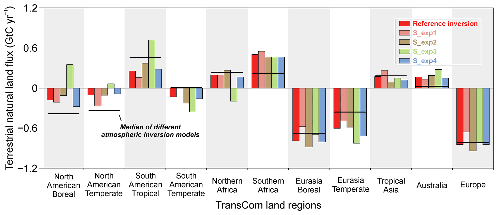
Figure 9Terrestrial natural land fluxes over the 11 TransCom land regions derived from sensitivity inversions for 2015. The results of the reference inversion and four sensitivity inversions (please see Table 2) are represented by bars denoting the posterior natural land fluxes (i.e., terrestrial biospheric + fire fluxes) in 2015 for each TransCom land region; the black lines represent the median values of all six inversion estimates shown in Fig. 5 over the corresponding region and period.
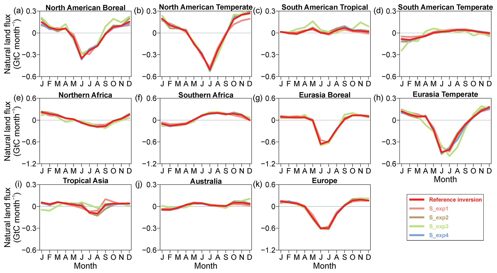
Figure 10Seasonal cycle amplitudes of natural land fluxes over the 11 TransCom land regions derived from sensitivity inversions for 2015. The results of the reference inversion and four sensitivity inversions (please see Table 2) are represented by solid curves denoting the posterior natural land fluxes (i.e., terrestrial biospheric + fire fluxes) in 2015; the colors are the same as those shown in Fig. 9.
4.2 Limitations and future perspectives
Atmospheric inversions are inherently ill-constrained due to the sparseness and uneven distribution of CO2 observations; additionally, these shortcomings are exacerbated by uncertainties in the process by which fluxes are associated with CO2 concentrations in atmospheric transport model simulation. In the regions and months that lack adequate quality observations, the prior information tends to be given more weight when estimating fluxes through inversion. Given the global optimization strategy of atmospheric inversions, the uncertainties associated with flux estimates over a given region can be propagated into another region representing a residual resulting from matching global observational constraints. Our analysis suggests that regional and monthly flux estimations are divergent across different atmospheric inversion models and even among the results of the same model under different configurations, although these monthly flux estimates can be integrated to estimate consistent global fluxes in line with the atmospheric growth rate of CO2. Our sensitivity inversions further revealed the considerable sensitivities of the regional inversion fluxes to the prior fluxes and their uncertainties, thus illustrating the difficulties associated with the consistent optimization of carbon fluxes from the global to the regional scale.
The ensemble methods such as 4D-LETKF used in this study have a major advantage over the adjoint-based variational methods (e.g., 4D-Var) in system development simplification, but the limited ensemble size and the short spatiotemporal localization window could reduce the estimation accuracy when there is a lack of sufficient CO2 observations (Chatterjee and Michalak, 2013; Liu et al., 2016). The 4D-Var method uses an adjoint model to compute the sensitivity of CO2 concentrations to surface fluxes, typically associated with a long data-assimilation window of years (e.g., Chevallier et al., 2005; Baker et al., 2006; Liu et al., 2016), which is accurate but computationally expensive. The 4D-LETKF algorithm relates surface carbon fluxes to CO2 observations through ensemble simulations upon a short data-assimilation window of hours to months (e.g., Kang et al., 2011; Peters et al., 2005; Bruhwiler et al., 2005). The 4D-LETKF algorithm was designed for easy implementation and computational efficiency (Hunt et al., 2007), making it easier and faster to use in high-dimensional assimilation systems than the 4D-Var method.
The explicit localization scheme in space and time for 4D-LETKF ensures the accuracy and efficiency of flux estimation based on a moderate size of ensemble members (Miyoshi and Yamane, 2007), especially over regions with sufficient observations. For example, the 4D-LETKF algorithm can achieve carbon fluxes comparable to 4D-Var over regions with dense CO2 observations (Liu et al., 2016). However, over observation-sparse regions, the localization scheme of 4D-LETKF makes it difficult to optimize fluxes effectively, while the 4D-Var method can optimize carbon fluxes based on observations over a broad region where CO2 concentrations are sensitive to fluxes. While increasing the duration of the data-assimilation window and localization length can improve 4D-LETKF performance in this case, it can however impose a heavy computational burden. Alternatively, several ensemble Kalman filter studies estimated carbon fluxes for ecoregions, which reduced the system dimensions to minimize the impacts of sampling errors and the lack of observational constraints on inversions (Peters et al., 2005; Feng et al., 2009). In the future, with the increased availability of satellite CO2 observations, the 4D-LETKF algorithm has the potential to play a more important role in grid-scale inversions.
Although our inversion system exhibited a good performance based on the evaluations against independent observations, regional-scale uncertainties still exist due to the inversion model limitations discussed above. The development of an atmospheric inversion system is a continuing effort that can benefit from developing new algorithms to improve transport model simulations and data assimilations and from increasing CO2 observation availabilities for data constraints and evaluation processes. The future development of our inversion system will include the following two aspects. (1) We aim to optimize the inversion system configuration, including the data-assimilation window and localization length, which are currently empirically designed based on previous literature and simplified sensitivity tests. A longer data-assimilation window or localization length could increase the amount of observation data used to constrain local fluxes; however, an appropriate configuration must be determined through comprehensive sensitivity experiments and evaluations, which are time-consuming but will be considered in future work. (2) We hope to improve the regional and seasonal representativeness of the utilized prior fluxes, especially those over regions that lack valid CO2 observations (e.g., the northern high latitudes and the tropics). Biogeochemical models that integrate process-based modules and multiple observations can be used to improve the prior biospheric fluxes and help to reduce model biases when simulating CO2 over mid- to high latitudes. The anthropogenic and biomass burning fluxes were prescribed in our inversion system, and these fluxes could be improved based on other inversion production chains to assimilate satellite retrievals of co-emitted short-lived reactive species, such as nitrogen dioxide (NO2) (Zheng et al., 2020) and carbon monoxide (CO) (Liu et al., 2017; Zheng et al., 2021).
Atmospheric inversions have the potential to significantly improve our understanding of the carbon cycle at the global and regional scales given their ability to integrate both prior information and atmospheric observations. Here, we developed a Bayesian atmospheric inversion system based on the 4D-LETKF algorithm coupled with the GEOS-Chem model; this system was constrained by OCO-2 XCO2 retrievals. To the best of our knowledge, this work represents the first time that the 4D-LETKF algorithm was adapted to a global carbon inversion system that assimilated OCO-2 data. With this newly developed inversion system, we inferred global gridded carbon fluxes from the latest OCO-2 V10r retrievals and investigated their magnitudes, variations, and partitioning schemes to understand the global and regional carbon budgets between 2015 and 2020. The resulting inversion-based carbon budgets agreed with the NOAA-observed CO2 atmospheric growth rates and substantially improved the modeled CO2 concentrations across latitudinal bands compared with the independent ground- and aircraft-based observations. Our global and regional carbon flux inversion estimates were broadly consistent with the other state-of-the-art atmospheric inversion models and the ensemble estimates derived from GCB2021, although discrepancies were still evident in the partitioning schemes between the natural land and ocean fluxes and the amplitude of the seasonal flux cycle over the TransCom land regions; these discrepancies could mainly be attributed to the sparse observational constraints resulting from the sampling and retrieval biases of the OCO-2 satellite and the divergent prior fluxes used in different inversion systems. We further investigated the robustness of and uncertainties in our inversion results through four sensitivity inversion tests that varied with regard to the utilized prior fluxes, applied uncertainties, and data-assimilation window length; the results indicated that the reference inversion results represented the optimal configuration in the current inversion framework. Additionally, our sensitivity inversions suggested that regions in which OCO-2 coverage is lacking are sensitive to the prior flux configuration, especially the tropics and northern high latitudes. The sensitivity inversion evaluations, as well as the comparisons with previous inversion models and data products, highlighted the dedicated future developmental direction of our atmospheric inversion system, representing a continuous and ongoing effort.
The inversion datasets generated in this study are available from the corresponding author on reasonable request.
The supplement related to this article is available online at: https://doi.org/10.5194/acp-22-10769-2022-supplement.
BZ designed the study and wrote the paper. YK performed the atmospheric inversion experiments, carried out the analysis, and prepared the initial draft. All of the authors provided research ideas, participated in the interpretation and discussion of the inversion results, and contributed to the writing and editing of the paper.
The contact author has declared that none of the authors has any competing interests.
Publisher’s note: Copernicus Publications remains neutral with regard to jurisdictional claims in published maps and institutional affiliations.
This work has been funded by the Young Elite Scientists Sponsorship Program by CAST (YESS20200135), the Scientific Research Start-up Funds (QD2021024C) from Tsinghua Shenzhen International Graduate School, and the National Natural Science Foundation of China (41921005). The OCO-2 retrievals were produced by the OCO-2 project at the Jet Propulsion Laboratory, California Institute of Technology, and obtained from the OCO-2 data archive maintained by NASA's Goddard Earth Science Data and Information Services Center. The authors would like to thank Ed Dlugokencky, Colm Sweeney, Ken Schuldt, Kathryn McKain, Bianca Baier, Anna Karion, Kathryn McKain, John B. Miller, and Charles E. Miller from NOAA, Kenneth Davis from Pennsylvania State University, and Steve Wofsy, Bruce Daube, and Roisin Commane from Harvard University for providing the in situ and aircraft CO2 measurement data. Additionally, we would like to thank all of the other contributors of the ObsPack data product. Andy Jacobson from NOAA and Andrew Schuh from Colorado State University provided the ObsPack diagnostic tools. The authors would also like to thank the GEOS-Chem team for providing the GEOS-Chem transport model code and manuals.
This research was supported by the Young Elite Scientists Sponsorship Program by CAST (grant no. YESS20200135), Scientific Research Start-up Funds (grant no. QD2021024C) from Tsinghua Shenzhen International Graduate School, and the National Natural Science Foundation of China (grant no. 41921005).
This paper was edited by Abhishek Chatterjee and reviewed by two anonymous referees.
Baker, D. F., Doney, S. C., and Schimel, D. S.: Variational data assimilation for atmospheric CO2, Tellus B, 58, 359–365, https://doi.org/10.1111/j.1600-0889.2006.00218.x, 2006.
Bastos, A., O'Sullivan, M., Ciais, P., Makowski, D., Sitch, S., Friedlingstein, P., Chevallier, F., Rödenbeck, C., Pongratz, J., Luijkx, I. T., Patra, P. K., Peylin, P., Canadell, J. G., Lauerwald, R., Li, W., Smith, N. E., Peters, W., Goll, D. S., Jain, A. K., Kato, E., Lienert, S., Lombardozzi, D. L., Haverd, V., Nabel, J. E. M. S., Poulter, B., Tian, H., Walker, A. P., and Zaehle, S.: Sources of Uncertainty in Regional and Global Terrestrial CO2 Exchange Estimates, Global Biogeochem. Cy., 34, e2019GB006393, https://doi.org/10.1029/2019GB006393, 2020.
Basu, S., Baker, D. F., Chevallier, F., Patra, P. K., Liu, J., and Miller, J. B.: The impact of transport model differences on CO2 surface flux estimates from OCO-2 retrievals of column average CO2, Atmos. Chem. Phys., 18, 7189–7215, https://doi.org/10.5194/acp-18-7189-2018, 2018.
Bey, I., Jacob, D. J., Yantosca, R. M., Logan, J. A., Field, B. D., Fiore, A. M., Li, Q., Liu, H. Y., Mickley, L. J., and Schultz, M. G.: Global modeling of tropospheric chemistry with assimilated meteorology: Model description and evaluation, J. Geophys. Res.-Atmos., 106, 23073–23095, https://doi.org/10.1029/2001JD000807, 2001.
Bruhwiler, L. M. P., Michalak, A. M., Peters, W., Baker, D. F., and Tans, P.: An improved Kalman Smoother for atmospheric inversions, Atmos. Chem. Phys., 5, 2691–2702, https://doi.org/10.5194/acp-5-2691-2005, 2005.
Canadell, J. G., Monteiro, P. M. S., Costa, M. H., Cotrim da Cunha, L., Cox, P. M., Eliseev, A. V., Henson, S., Ishii, M., Jaccard, S., Koven, C., Lohila, A., Patra, P. K., Piao, S., Rogelj, J., Syampungani, S., Zaehle, S., and Zickfeld, K.: Global Carbon and other Biogeochemical Cycles and Feedbacks, in: Climate Change 2021: The Physical Science Basis. Contribution of Working Group I to the Sixth Assessment Report of the Intergovernmental Panel on Climate Change, edited by: Masson-Delmotte, V., Zhai, P., Pirani, A., Connors, S. L., Péan, C., Berger, S., Caud, N., Chen, Y., Goldfarb, L., Gomis, M. I., Huang, M., Leitzell, K., Lonnoy, E., Matthews, J. B. R., Maycock, T. K., Waterfield, T., Yelekçi, O., Yu, R., and Zhou, B., Cambridge University Press, Cambridge, United Kingdom and New York, NY, USA, 673–816, https://doi.org/10.1017/9781009157896.007, 2021.
Chatterjee, A. and Michalak, A. M.: Technical Note: Comparison of ensemble Kalman filter and variational approaches for CO2 data assimilation, Atmos. Chem. Phys., 13, 11643–11660, https://doi.org/10.5194/acp-13-11643-2013, 2013.
Chevallier, F., Fisher, M., Peylin, P., Serrar, S., Bousquet, P., Bréon, F. M., Chédin, A., and Ciais, P.: Inferring CO2 sources and sinks from satellite observations: Method and application to TOVS data, J. Geophys. Res.-Atmos., 110, D24309, https://doi.org/10.1029/2005JD006390, 2005.
Chevallier, F., Palmer, P. I., Feng, L., Boesch, H., O'Dell, C. W., and Bousquet, P.: Toward robust and consistent regional CO2 flux estimates from in situ and spaceborne measurements of atmospheric CO2, Geophys. Res. Lett., 41, 1065–1070, https://doi.org/10.1002/2013GL058772, 2014.
Chevallier, F., Remaud, M., O'Dell, C. W., Baker, D., Peylin, P., and Cozic, A.: Objective evaluation of surface- and satellite-driven carbon dioxide atmospheric inversions, Atmos. Chem. Phys., 19, 14233–14251, https://doi.org/10.5194/acp-19-14233-2019, 2019.
Ciais, P., Rayner, P., Chevallier, F., Bousquet, P., Logan, M., Peylin, P., and Ramonet, M.: Atmospheric inversions for estimating CO2 fluxes: methods and perspectives, Clim. Chang., 103, 69–92, https://doi.org/10.1007/s10584-010-9909-3, 2010.
Ciais, P., Tan, J., Wang, X., Roedenbeck, C., Chevallier, F., Piao, S. L., Moriarty, R., Broquet, G., Le Quéré, C., Canadell, J. G., Peng, S., Poulter, B., Liu, Z., and Tans, P.: Five decades of northern land carbon uptake revealed by the interhemispheric CO2 gradient, Nature, 568, 221–225, https://doi.org/10.1038/s41586-019-1078-6, 2019.
Ciais, P., Bastos, A., Chevallier, F., Lauerwald, R., Poulter, B., Canadell, J. G., Hugelius, G., Jackson, R. B., Jain, A., Jones, M., Kondo, M., Luijkx, I. T., Patra, P. K., Peters, W., Pongratz, J., Petrescu, A. M. R., Piao, S., Qiu, C., Von Randow, C., Regnier, P., Saunois, M., Scholes, R., Shvidenko, A., Tian, H., Yang, H., Wang, X., and Zheng, B.: Definitions and methods to estimate regional land carbon fluxes for the second phase of the REgional Carbon Cycle Assessment and Processes Project (RECCAP-2), Geosci. Model Dev., 15, 1289–1316, https://doi.org/10.5194/gmd-15-1289-2022, 2022.
Cooperative Global Atmospheric Data Integration Project: Multi-laboratory compilation of atmospheric carbon dioxide data for the period 1957–2020; obspack_co2_1_GLOBALVIEWplus_v7.0_2021-08-18, NOAA Earth System Research Laboratory, Global Monitoring Laboratory, https://doi.org/10.25925/20210801, 2021.
Crowell, S., Baker, D., Schuh, A., Basu, S., Jacobson, A. R., Chevallier, F., Liu, J., Deng, F., Feng, L., McKain, K., Chatterjee, A., Miller, J. B., Stephens, B. B., Eldering, A., Crisp, D., Schimel, D., Nassar, R., O'Dell, C. W., Oda, T., Sweeney, C., Palmer, P. I., and Jones, D. B. A.: The 2015–2016 carbon cycle as seen from OCO-2 and the global in situ network, Atmos. Chem. Phys., 19, 9797–9831, https://doi.org/10.5194/acp-19-9797-2019, 2019.
Deng, F., Jones, D. B. A., Henze, D. K., Bousserez, N., Bowman, K. W., Fisher, J. B., Nassar, R., O'Dell, C., Wunch, D., Wennberg, P. O., Kort, E. A., Wofsy, S. C., Blumenstock, T., Deutscher, N. M., Griffith, D. W. T., Hase, F., Heikkinen, P., Sherlock, V., Strong, K., Sussmann, R., and Warneke, T.: Inferring regional sources and sinks of atmospheric CO2 from GOSAT XCO2 data, Atmos. Chem. Phys., 14, 3703–3727, https://doi.org/10.5194/acp-14-3703-2014, 2014.
Eldering, A., Wennberg, P. O., Crisp, D., Schimel, D. S., Gunson, M. R., Chatterjee, A., Liu, J., Schwandner, F. M., Sun, Y., O'Dell, C. W., Frankenberg, C., Taylor, T., Fisher, B., Osterman, G. B., Wunch, D., Hakkarainen, J., Tamminen, J., and Weir, B.: The Orbiting Carbon Observatory-2 early science investigations of regional carbon dioxide fluxes, Science, 358, eaam5745, https://doi.org/10.1126/science.aam5745, 2017.
Feng, L., Palmer, P. I., Bösch, H., and Dance, S.: Estimating surface CO2 fluxes from space-borne CO2 dry air mole fraction observations using an ensemble Kalman Filter, Atmos. Chem. Phys., 9, 2619–2633, https://doi.org/10.5194/acp-9-2619-2009, 2009.
Friedlingstein, P., Jones, M. W., O'Sullivan, M., Andrew, R. M., Bakker, D. C. E., Hauck, J., Le Quéré, C., Peters, G. P., Peters, W., Pongratz, J., Sitch, S., Canadell, J. G., Ciais, P., Jackson, R. B., Alin, S. R., Anthoni, P., Bates, N. R., Becker, M., Bellouin, N., Bopp, L., Chau, T. T. T., Chevallier, F., Chini, L. P., Cronin, M., Currie, K. I., Decharme, B., Djeutchouang, L. M., Dou, X., Evans, W., Feely, R. A., Feng, L., Gasser, T., Gilfillan, D., Gkritzalis, T., Grassi, G., Gregor, L., Gruber, N., Gürses, Ö., Harris, I., Houghton, R. A., Hurtt, G. C., Iida, Y., Ilyina, T., Luijkx, I. T., Jain, A., Jones, S. D., Kato, E., Kennedy, D., Klein Goldewijk, K., Knauer, J., Korsbakken, J. I., Körtzinger, A., Landschützer, P., Lauvset, S. K., Lefèvre, N., Lienert, S., Liu, J., Marland, G., McGuire, P. C., Melton, J. R., Munro, D. R., Nabel, J. E. M. S., Nakaoka, S.-I., Niwa, Y., Ono, T., Pierrot, D., Poulter, B., Rehder, G., Resplandy, L., Robertson, E., Rödenbeck, C., Rosan, T. M., Schwinger, J., Schwingshackl, C., Séférian, R., Sutton, A. J., Sweeney, C., Tanhua, T., Tans, P. P., Tian, H., Tilbrook, B., Tubiello, F., van der Werf, G. R., Vuichard, N., Wada, C., Wanninkhof, R., Watson, A. J., Willis, D., Wiltshire, A. J., Yuan, W., Yue, C., Yue, X., Zaehle, S., and Zeng, J.: Global Carbon Budget 2021, Earth Syst. Sci. Data, 14, 1917–2005, https://doi.org/10.5194/essd-14-1917-2022, 2022.
Gaubert, B., Stephens, B. B., Basu, S., Chevallier, F., Deng, F., Kort, E. A., Patra, P. K., Peters, W., Rödenbeck, C., Saeki, T., Schimel, D., Van der Laan-Luijkx, I., Wofsy, S., and Yin, Y.: Global atmospheric CO2 inverse models converging on neutral tropical land exchange, but disagreeing on fossil fuel and atmospheric growth rate, Biogeosciences, 16, 117–134, https://doi.org/10.5194/bg-16-117-2019, 2019.
Gurney, K. R., Law, R. M., Denning, A. S., Rayner, P. J., Baker, D., Bousquet, P., Bruhwiler, L., Chen, Y.-H., Ciais, P., Fan, S., Fung, I. Y., Gloor, M., Heimann, M., Higuchi, K., John, J., Maki, T., Maksyutov, S., Masarie, K., Peylin, P., Prather, M., Pak, B. C., Randerson, J., Sarmiento, J., Taguchi, S., Takahashi, T., and Yuen, C.-W.: Towards robust regional estimates of CO2 sources and sinks using atmospheric transport models, Nature, 415, 626–630, https://doi.org/10.1038/415626a, 2002.
Gurney, K. R., Law, R. M., Denning, A. S., Rayner, P. J., Baker, D., Bousquet, P., Bruhwiler, L., Chen, Y.-H., Ciais, P., Fan, S., Fung, I. Y., Gloor, M., Heimann, M., Higuchi, K., John, J., Kowalczyk, E., Maki, T., Maksyutov, S., Peylin, P., Prather, M., Pak, B. C., Sarmiento, J., Taguchi, S., Takahashi, T., and Yuen, C.-W.: TransCom 3 CO2 inversion intercomparison: 1. Annual mean control results and sensitivity to transport and prior flux information, Tellus B, 55, 555–579, https://doi.org/10.3402/tellusb.v55i2.16728, 2003.
Haynes, K. D., Baker, I. T., and Denning, A. S.: SiB4 Modeled Global 0.5-Degree Hourly Carbon Fluxes and Productivity, 2000–2018, ORNL DAAC, Oak Ridge, Tennessee, USA, https://doi.org/10.3334/ORNLDAAC/1847, 2021.
Houweling, S., Baker, D., Basu, S., Boesch, H., Butz, A., Chevallier, F., Deng, F., Dlugokencky, E. J., Feng, L., Ganshin, A., Hasekamp, O., Jones, D., Maksyutov, S., Marshall, J., Oda, T., O'Dell, C. W., Oshchepkov, S., Palmer, P. I., Peylin, P., Poussi, Z., Reum, F., Takagi, H., Yoshida, Y., and Zhuravlev, R.: An intercomparison of inverse models for estimating sources and sinks of CO2 using GOSAT measurements, J. Geophys. Res.-Atmos., 120, 5253–5266, https://doi.org/10.1002/2014JD022962, 2015.
Houtekamer, P. L. and Zhang, F.: Review of the Ensemble Kalman Filter for Atmospheric Data Assimilation, Mon. Weather Rev., 144, 4489–4532, https://doi.org/10.1175/MWR-D-15-0440.1, 2016.
Hunt, B. R., Kostelich, E. J., and Szunyogh, I.: Efficient data assimilation for spatiotemporal chaos: A local ensemble transform Kalman filter, Physica D, 230, 112–126, https://doi.org/10.1016/j.physd.2006.11.008, 2007.
Jacobson, A. R., Schuldt, K. N., Miller, J. B., Oda, T., Tans, P., Arlyn, A., Mund, J., Ott, L., Collatz, G. J., Aalto, T., Afshar, S., Aikin, K., Aoki, S., Apadula, F., Baier, B., Bergamaschi, P., Beyersdorf, A., Biraud, S. C., Bollenbacher, A., Bowling, D., Brailsford, G., Abshire, J. B., Chen, G., Huilin, C., Lukasz, C., Sites, C., Colomb, A., Conil, S., Cox, A., Cristofanelli, P., Cuevas, E., Curcoll, R., Sloop, C. D., Davis, K., Wekker, S. D., Delmotte, M., DiGangi, J. P., Dlugokencky, E., Ehleringer, J., Elkins, J. W., Emmenegger, L., Fischer, M. L., Forster, G., Frumau, A., Galkowski, M., Gatti, L. V., Gloor, E., Griffis, T., Hammer, S., Haszpra, L., Hatakka, J., Heliasz, M., Hensen, A., Hermanssen, O., Hintsa, E., Holst, J., Jaffe, D., Karion, A., Kawa, S. R., Keeling, R., Keronen, P., Kolari, P., Kominkova, K., Kort, E., Krummel, P., Kubistin, D., Labuschagne, C., Langenfelds, R., Laurent, O., Laurila, T., Lauvaux, T., Law, B., Lee, J., Lehner, I., Leuenberger, M., Levin, I., Levula, J., Lin, J., Lindauer, M., Loh, Z., Lopez, M., Luijkx, I. T., Myhre, C. L., Machida, T., Mammarella, I., Manca, G., Manning, A., Manning, A., Marek, M. V., Marklund, P., Martin, M. Y., Matsueda, H., McKain, K., Meijer, H., Meinhardt, F., Miles, N., Miller, C. E., Mölder, M., Montzka, S., Moore, F., Josep-Anton, M., Morimoto, S., Munger, B., Jaroslaw, N., Newman, S., Nichol, S., Niwa, Y., O'Doherty, S., Mikaell, O.-L., Paplawsky, B., Peischl, J., Peltola, O., Jean-Marc, P., Piper, S., Plass-Dölmer, C., Ramonet, M., ReyesSanchez, E., Richardson, S., Riris, H., Ryerson, T., Saito, K., Sargent, M., Sasakawa, M., Sawa, Y., Say, D., Scheeren, B., Schmidt, M., Schmidt, A., Schumacher, M., Shepson, P., Shook, M., Stanley, K., Steinbacher, M., Stephens, B., Sweeney, C., Thoning, K., Torn, M.,Turnbull, J., Tørseth, K., Bulk, P. V. D., Dinther, D. V., Vermeulen, A., Viner, B., Vitkova, G., Walker, S., Weyrauch, D., Wofsy, S., Worthy, D., Dickon, Y., and Miroslaw, Z.: CarbonTracker CT2019B, https://doi.org/10.25925/20201008, 2020.
Jiang, F., Wang, H., Chen, J. M., Ju, W., Tian, X., Feng, S., Li, G., Chen, Z., Zhang, S., Lu, X., Liu, J., Wang, H., Wang, J., He, W., and Wu, M.: Regional CO2 fluxes from 2010 to 2015 inferred from GOSAT XCO2 retrievals using a new version of the Global Carbon Assimilation System, Atmos. Chem. Phys., 21, 1963–1985, https://doi.org/10.5194/acp-21-1963-2021, 2021.
Kang, J.-S., Kalnay, E., Liu, J., Fung, I., Miyoshi, T., and Ide, K.: “Variable localization” in an ensemble Kalman filter: application to the carbon cycle data assimilation, J. Geophys. Res., 116, D09110, https://doi.org/10.1029/2010JD014673, 2011.
Liu, J., Bowman, K. W., and Lee, M.: Comparison between the Local Ensemble Transform Kalman Filter (LETKF) and 4D-Var in atmospheric CO2 flux inversion with the Goddard Earth Observing System-Chem model and the observation impact diagnostics from the LETKF, J. Geophys. Res.-Atmos., 121, 13066–13087, https://doi.org/10.1002/2016JD025100, 2016.
Liu, J., Bowman, K. W., Schimel, D. S., Parazoo, N. C., Jiang, Z., Lee, M., Bloom, A. A., Wunch, D., Frankenberg, C., Sun, Y., O'Dell, C. W., Gurney, K. R., Menemenlis, D., Gierach, M., Crisp, D., and Eldering, A.: Contrasting carbon cycle responses of the tropical continents to the 2015–2016 El Niño, Science, 358, eaam5690, https://doi.org/10.1126/science.aam5690, 2017.
Liu, Y., Kalnay, E., Zeng, N., Asrar, G., Chen, Z., and Jia, B.: Estimating surface carbon fluxes based on a local ensemble transform Kalman filter with a short assimilation window and a long observation window: an observing system simulation experiment test in GEOS-Chem 10.1, Geosci. Model Dev., 12, 2899–2914, https://doi.org/10.5194/gmd-12-2899-2019, 2019.
Liu, Z., Ciais, P., Deng, Z., Lei, R., Davis, S. J., Feng, S., Zheng, B., Cui, D., Dou, X., Zhu, B., Guo, R., Ke, P., Sun, T., Lu, C., He, P., Wang, Y., Yue, X., Wang, Y., Lei, Y., Zhou, H., Cai, Z., Wu, Y., Guo, R., Han, T., Xue, J., Boucher, O., Boucher, E., Chevallier, F., Tanaka, K., Wei, Y., Zhong, H., Kang, C., Zhang, N., Chen, B., Xi, F., Liu, M., Bréon, F.-M., Lu, Y., Zhang, Q., Guan, D., Gong, P., Kammen, D. M., He, K., and Schellnhuber, H. J.: Near-real-time monitoring of global CO2 emissions reveals the effects of the COVID-19 pandemic, Nat. Commun., 11, 5172, https://doi.org/10.1038/s41467-020-18922-7, 2020.
Liu, J., Baskaran, L., Bowman, K., Schimel, D., Bloom, A. A., Parazoo, N. C., Oda, T., Carroll, D., Menemenlis, D., Joiner, J., Commane, R., Daube, B., Gatti, L. V., McKain, K., Miller, J., Stephens, B. B., Sweeney, C., and Wofsy, S.: Carbon Monitoring System Flux Net Biosphere Exchange 2020 (CMS-Flux NBE 2020), Earth Syst. Sci. Data, 13, 299–330, https://doi.org/10.5194/essd-13-299-2021, 2021.
Masarie, K. A., Peters, W., Jacobson, A. R., and Tans, P. P.: ObsPack: a framework for the preparation, delivery, and attribution of atmospheric greenhouse gas measurements, Earth Syst. Sci. Data, 6, 375–384, https://doi.org/10.5194/essd-6-375-2014, 2014.
Miyazaki, K., Maki, T., Patra, P., and Nakazawa, T.: Assessing the impact of satellite, aircraft, and surface observations on CO2 flux estimation using an ensemblebased 4-D data assimilation system, J. Geophys. Res., 116, D16306, https://doi.org/10.1029/2010JD015366, 2011.
Miyoshi, T. and Yamane, S.: Local Ensemble Transform Kalman Filtering with an AGCM at a T159/L48 Resolution, Mon. Weather Rev., 135, 3841–3861, https://doi.org/10.1175/2007MWR1873.1, 2007.
Nassar, R., Napier-Linton, L., Gurney, K. R., Andres, R. J., Oda, T., Vogel, F. R., and Deng, F.: Improving the temporal and spatial distribution of CO2 emissions from global fossil fuel emission data sets, J. Geophys. Res.-Atmos., 118, 917–933, https://doi.org/10.1029/2012JD018196, 2013.
OCO-2 Science Team/Michael Gunson and Annmarie Eldering: OCO-2 Level 2 bias-corrected XCO2 and other select fields from the full-physics retrieval aggregated as daily files, Retrospective processing V10r, Greenbelt, MD, USA, Goddard Earth Sciences Data and Information Services Center (GES DISC), https://doi.org/10.5067/E4E140XDMPO2, 2020.
Oda, T., Maksyutov, S., and Andres, R. J.: The Open-source Data Inventory for Anthropogenic CO2, version 2016 (ODIAC2016): a global monthly fossil fuel CO2 gridded emissions data product for tracer transport simulations and surface flux inversions, Earth Syst. Sci. Data, 10, 87–107, https://doi.org/10.5194/essd-10-87-2018, 2018.
O'Dell, C. W., Eldering, A., Wennberg, P. O., Crisp, D., Gunson, M. R., Fisher, B., Frankenberg, C., Kiel, M., Lindqvist, H., Mandrake, L., Merrelli, A., Natraj, V., Nelson, R. R., Osterman, G. B., Payne, V. H., Taylor, T. E., Wunch, D., Drouin, B. J., Oyafuso, F., Chang, A., McDuffie, J., Smyth, M., Baker, D. F., Basu, S., Chevallier, F., Crowell, S. M. R., Feng, L., Palmer, P. I., Dubey, M., García, O. E., Griffith, D. W. T., Hase, F., Iraci, L. T., Kivi, R., Morino, I., Notholt, J., Ohyama, H., Petri, C., Roehl, C. M., Sha, M. K., Strong, K., Sussmann, R., Te, Y., Uchino, O., and Velazco, V. A.: Improved retrievals of carbon dioxide from Orbiting Carbon Observatory-2 with the version 8 ACOS algorithm, Atmos. Meas. Tech., 11, 6539–6576, https://doi.org/10.5194/amt-11-6539-2018, 2018.
Peters, W., Miller, J., Whitaker, J., Denning, S., Hirsch, A., Krol, M., Zupanski, D., Bruhwiler, L., and Tans, P.: An ensemble data assimilation system to estimate CO2 surface fluxes from atmospheric trace gas observations, J. Geophys. Res., 110, D24304, https://doi.org/10.1029/2005JD006157, 2005.
Peters, W., Jacobson, A. R., Sweeney, C., Andrews, A. E., Conway, T. J., Masarie, K., Miller, J. B., Bruhwiler, L. M. P., Pétron, G., Hirsch, A. I., Worthy, D. E. J., van der Werf, G. R., Randerson, J. T., Wennberg, P. O., Krol, M. C., and Tans, P. P.: An atmospheric perspective on North American carbon dioxide exchange: CarbonTracker, P. Natl. Acad. Sci. USA., 104, 18925–18930, https://doi.org/10.1073/pnas.0708986104, 2007.
Peylin, P., Law, R. M., Gurney, K. R., Chevallier, F., Jacobson, A. R., Maki, T., Niwa, Y., Patra, P. K., Peters, W., Rayner, P. J., Rödenbeck, C., van der Laan-Luijkx, I. T., and Zhang, X.: Global atmospheric carbon budget: results from an ensemble of atmospheric CO2 inversions, Biogeosciences, 10, 6699–6720, https://doi.org/10.5194/bg-10-6699-2013, 2013.
Rödenbeck, C., Zaehle, S., Keeling, R., and Heimann, M.: History of El Niño impacts on the global carbon cycle 1957–2017: a quantification from atmospheric CO2 data, Philos. T. Roy. Soc. B, 373, 20170303, https://doi.org/10.1098/rstb.2017.0303, 2018.
Takahashi, T., Sutherland, S. C., Wanninkhof, R., Sweeney, C., Feely, R. A., Chipman, D. W., Hales, B., Friederich, G., Chavez, F., Sabine, C., Watson, A., Bakker, D. C. E., Schuster, U., Metzl, N., Yoshikawa-Inoue, H., Ishii, M., Midorikawa, T., Nojiri, Y., Körtzinger, A., Steinhoff, T., Hoppema, M., Olafsson, J., Arnarson, T. S., Tilbrook, B., Johannessen, T., Olsen, A., Bellerby, R., Wong, C. S., Delille, B., Bates, N. R., and de Baar, H. J. W.: Climatological mean and decadal change in surface ocean pCO2, and net sea–air CO2 flux over the global oceans, Deep-Sea Res. Pt. II, 56, 554–577, https://doi.org/10.1016/j.dsr2.2008.12.009, 2009.
Thompson, R. L., Patra, P. K., Chevallier, F., Maksyutov, S., Law, R. M., Ziehn, T., van der Laan-Luijkx, I. T., Peters, W., Ganshin, A., Zhuravlev, R., Maki, T., Nakamura, T., Shirai, T., Ishizawa, M., Saeki, T., Machida, T., Poulter, B., Canadell, J. G., and Ciais, P.: Top-down assessment of the Asian carbon budget since the mid 1990s, Nat. Commun., 7, 10724, https://doi.org/10.1038/ncomms10724, 2016.
Tian, S., Wang, S., Bai, X., Luo, G., Li, Q., Yang, Y., Hu, Z., Li, C., and Deng, Y.: Global patterns and changes of carbon emissions from land use during 1992–2015, Environmental Science and Ecotechnology, 7, 100108, https://doi.org/10.1016/j.ese.2021.100108, 2021.
van der Werf, G. R., Randerson, J. T., Giglio, L., van Leeuwen, T. T., Chen, Y., Rogers, B. M., Mu, M., van Marle, M. J. E., Morton, D. C., Collatz, G. J., Yokelson, R. J., and Kasibhatla, P. S.: Global fire emissions estimates during 1997–2016, Earth Syst. Sci. Data, 9, 697–720, https://doi.org/10.5194/essd-9-697-2017, 2017.
Zheng, B., Geng, G., Ciais, P., Davis, S. J., Martin, R. V., Meng, J., Wu, N., Chevallier, F., Broquet, G., Boersma, F., van der A, R., Lin, J., Guan, D., Lei, Y., He, K., and Zhang, Q.: Satellite-based estimates of decline and rebound in China's CO2 emissions during COVID-19 pandemic, Sci. Adv., 6, eabd4998, https://doi.org/10.1126/sciadv.abd4998, 2020.
Zheng, B., Ciais, P., Chevallier, F., Chuvieco, E., Chen, Y., and Yang, H.: Increasing forest fire emissions despite the decline in global burned area, Sci. Adv., 7, eabh2646, https://doi.org/10.1126/sciadv.abh2646, 2021.
Zhang, S., Zheng, X., Chen, J. M., Chen, Z., Dan, B., Yi, X., Wang, L., and Wu, G.: A global carbon assimilation system using a modified ensemble Kalman filter, Geosci. Model Dev., 8, 805–816, https://doi.org/10.5194/gmd-8-805-2015, 2015.