the Creative Commons Attribution 4.0 License.
the Creative Commons Attribution 4.0 License.
 | 23 Aug 2022
Evaluation of correlated Pandora column NO2 and in situ surface NO2 measurements during GMAP campaign
Donghee Kim
Hyunkee Hong
Deok-Rae Kim
Jeong-Ah Yu
Kwangyul Lee
Hanlim Lee
Daewon Kim
Jinkyu Hong
Hyun-Young Jo
To validate the Geostationary Environment Monitoring Spectrometer (GEMS), the GEMS Map of Air Pollution (GMAP) campaign was conducted during 2020–2021 by integrating Pandora Asia Network, aircraft, and in situ measurements. In the present study, GMAP-2020 measurements were applied to evaluate urban air quality and explore the synergy of Pandora column (PC) NO2 measurements and surface in situ (SI) NO2 measurements for Seosan, South Korea, where large point source (LPS) emissions are densely clustered. Due to the difficulty of interpreting the effects of LPS emissions on air quality downwind of Seosan using SI monitoring networks alone, we explored the combined analysis of both PC-NO2 and SI-NO2 measurements. Agglomerative hierarchical clustering using vertical meteorological variables combined with PC-NO2 and SI-NO2 yielded three distinct conditions: synoptic wind-dominant (SD), mixed (MD), and local wind-dominant (LD). These results suggest meteorology-dependent correlations between PC-NO2 and SI-NO2. Overall, yearly daytime mean (11:00–17:00 KST) PC-NO2 and SI-NO2 statistical data showed good linear correlations (); however, the differences in correlations were largely attributed to meteorological conditions. SD conditions characterized by higher wind speeds and advected marine boundary layer heights suppressed fluctuations in both PC-NO2 and SI-NO2, driving a uniform vertical NO2 structure with higher correlations, whereas under LD conditions, LPS plumes were decoupled from the surface or were transported from nearby cities, weakening correlations through anomalous vertical NO2 gradients. The discrepancies suggest that using either PC-NO2 or SI-NO2 observations alone involves a higher possibility of uncertainty under LD conditions or prevailing transport processes. However, under MD conditions, both pollution ventilation due to high surface wind speeds and daytime photochemical NO2 loss contributed to stronger correlations through a decline in both PC-NO2 and SI-NO2 towards noon. Thus, Pandora Asia Network observations collected over 13 Asian countries since 2021 can be utilized for detailed investigation of the vertical complexity of air quality, and the conclusions can be also applied when performing GEMS observation interpretation in combination with SI measurements.
- Article
(5779 KB) - Full-text XML
-
Supplement
(923 KB) - BibTeX
- EndNote


Rapid developments in environmental remote sensing have led to a new era of air quality observations, and recent hyperspectral data retrieval technologies have allowed for routine and accurate monitoring of air pollutants at high spatial and temporal resolution. In particular, the Geostationary Environment Monitoring Spectrometer (GEMS), which was launched on 18 February 2020, measures the total and tropospheric air pollutant columns hourly at spatial resolutions of 7 km × 8 km for gas and 3.5 km × 8 km for aerosols (Kim et al., 2020), facilitating the tracking of pollution transport from local to synoptic scales.
Recent studies have revealed the potential of satellite observations to evaluate surface air quality, particularly in regions with sparse air quality-monitoring networks. The main approach is to convert column density to surface concentrations using a shape factor of the ratio of the partial column () within the lowest layer (z0) to the total column (Ωtotal) (Zhao et al., 2019), as follows:
where S, C, and Δz0 are the surface concentration, column density, and lowest layer thickness, respectively. Acquiring accurate profile shape information is critical for determining the relationship between the column amount and surface concentration because the shape factor is spatiotemporally variable. Considering this, numerous studies have obtained close relationships using chemical transport model simulations, aircraft in situ measurements, and satellite observations with high correlation coefficients (R) of 0.7 or more, and used them to scale up surface NO2 to column NO2 (Wang and Christopher, 2003; Boersma et al., 2009; Lamsal et al., 2010). This strong correlation can be explained by the generally uniform planetary boundary layer height (PBLH), and by aerosol type and abundance, which is also the case for trace gases.
By contrast, the implications of weak correlations between column and surface measurements remain unclear. Engel-Cox et al. (2004) found a negative correlation of aerosol optical depth (AOD) and surface PM2.5 in northwestern USA, and explained it based on elevated haze decoupled from the surface. Thompson et al. (2019) examined weak correlations between Pandora column (PC) measurements and surface in situ (SI) observations of NO2 over the Yellow Sea during the Korea–US air quality (KORUS-AQ) field study, and suggested, as a possible reason, the transported non-uniform plumes originated in China and Seoul hundreds of meters above the ground from the surface layer. The estimated surface PM2.5 concentration was weakly correlated (R=0.4–0.49) with observed PM2.5 concentrations in Seoul because only PBLH was added to the multi-linear regression model to correlate AOD to surface PM2.5 (Kim et al., 2021). This effect may be related to the significant impact of long-range transport on PM2.5, with a contribution of up to 39 % in Seoul (Lee et al., 2021). Thus, the wide variability in the degree of correlation between PC–PM and SI–PM is closely related to vertical profile variability (Flynn et al., 2016).
It appears highly probable that several factors are responsible for the correlations between PC-NO2 and SI-NO2; therefore, it is necessary to improve our understanding of the degree of correlation through detailed measurements, including column concentration. In this study, we focused on the impact of meteorology and chemistry on correlation variability using PC, SI and aircraft measurements, and meteorological observations. Understanding vertical profile variability is also useful for evaluating the effects of various emissions on urban air quality, particularly in areas neighboring active large point source (LPS) emissions sites. Quantifying the impact of LPS emissions on downwind cities remains challenging due to the lack of three-dimensional (3D) measurements. Accurate vertical profile data are also useful for improving remote sensing retrieval algorithms because the profile shape contributes to the conversion of slant column density into vertical column density as part of the air mass factor.
In mid-2019, the Pandonia Global Network (PGN; https://pandonia-global-network.org, last access: 22 August 2022) was launched, with support from the National Aeronautics and Space Administration (NASA) and European Space Agency (ESA), to facilitate the validation and verification of low-orbit or geostationary environmental satellites. This network is attempting to expand air quality monitoring through integration with existing long-term air quality monitoring stations. Since 2020, the National Institute of Environmental Research, Economic and Social Commission for Asia and the Pacific, and Korea Environment Corporation have been extending the Pandora Asia Network to include 13 Asian countries, with support from the Korea International Cooperation Agency. The Pandora Asia Network is expected to be widely used to study urban air quality in Asia, which is increasingly deteriorating due to rapid economic growth.
As part of the GEMS Map of Air Pollution (GMAP) campaign, a suite of Pandora instruments was deployed in Seosan, a South Korean coastal city, from November 2020 to January 2021 (GMAP-2020), and we applied GMAP-2020 measurements to explore the synergy of PC observations when evaluating air quality over Seosan. Further results from this research project are also reported in this special issue, including GEMS validation and urban air quality evaluations based on Pandora, aircraft, surface flux, and in situ surface chemical measurements conducted during GMAP-2020.

Figure 1Map of sites used for Geostationary Environment Monitoring Spectrometer (GEMS) Map of Air Pollution (GMAP) campaigns conducted in (a) Seosan, South Korea in November 2020 to January 2021 (GMAP-2020), and (b) the Seoul metropolitan area from October 2021 to November 2021 (GMAP-2021). (a) Measurement sites around Seosan, the study area for the GMAP-2020 campaign. Red circles indicate Pandora column measurement sites including (b) Seosan Daehoji (PA1), Seosan Dongmun (PA2), Seosan city council (PA3), and Seosan super site (PA4). Blue triangles indicate large point sources (LPSs) including the Taean and Dangjin thermal power stations (LPS1 and LPS2, respectively), Hyundai steelworks (LPS3), and Daesan petrochemical complex (LPS4). Yellow squares indicate Automated Synoptic Observing System meteorological sites in Seosan (Met1), AWS (Met2), and buoy (Met3). Green squares indicate air quality monitoring (AQM) network stations including Padori (AQM1), Leewon (AQM2), Taean (AQM3), Daesan (AQM4), Seongyeon (AQM5), and Dongmoon (AQM6). In the right panel, the black line indicates the route used for car-based differential optical absorption spectroscopy (Car-DOAS) measurements and the blue dotted line indicates the horizontal domain of Geostationary Coastal and Air Pollution Events (GEO-CAPE) airborne simulator (GCAS) measurements taken during the GMAP-2021 campaign.
GEMS was launched on 19 February 2020; it is the first instrument to observe air quality from a geostationary Earth orbit. GEMS provides hourly air quality data on aerosols and gases at a spatial resolution of 7 km × 8 km. It is a scanning ultraviolet (UV)–visible spectrometer that observes key atmospheric constituents including O3, NO2, CO, SO2, CH2O, CHOCHO, aerosols, clouds, and UV indices. This mission heralded a new era of satellite air quality monitoring and will be joined by NASA's Tropospheric Emissions: Monitoring of Pollution (TEMPO) and ESA's Sentinel-4 to form the GEO Air Quality Constellation in ∼3 years, to cover the most polluted region in the Northern Hemisphere.
During GMAP-2020, Pandora instruments (PA1–PA4) were deployed near large point sources (LPS1–LPS4) in Seosan; in situ surface air quality monitoring systems (AQM1–AQM6) and meteorological observations (Met1–Met3) were also used in this study (see their locations in Fig. 1). Aircraft measurements were also used to validate GEMS and diagnose LPSs located in industrial areas surrounding Seosan. We explored the synergy of Pandora observations and SI measurements, based on measurements collected during GMAP-2020, by evaluating air quality in industrial Seosan (where LPSs are densely clustered). We particularly investigated the impacts of vertical profile and sub-pixel variability for trace gases and aerosols, for further GEMS validation. All measurement sites for both GMAP-2020 campaigns are indicated in Fig. 1.
3.1 Study area
Seosan, the target area of the GMAP-2020 campaign, is a small city with a population of 174 780 in 2017; it is accessed via three expressways to the east and four national highways cross the city. It is located in midwestern South Korea, and is affected by >300 emissions point sources including LPSs. Coal-fired power plants including Taean, Dangjin, the Hyundai Dangjin steelworks, and the Daesan petrochemistry industrial complex (LPS1–LPS4, respectively, in Fig. 1) have the highest emissions rates in South Korea. The Hyundai Dangjin steelworks (LPS3) and Taean and Dangjin power plants (LPS1 and LPS2) emit 10.5, 11, and 8.8 Gg of NOx per year, respectively. Although Seosan accounts for only 1.8 % of the population of Seoul, its NOx emissions (10.2 Gg yr−1) account for 13.2 % of its total NOx emissions. The transportation sector of Seosan is a far greater NOx source than the industrial sector of Seoul (ratio of 99:1); however, within Seosan, the industrial sector is on par with the transport sector (52:48; https://www.air.go.kr/en-main.do, last access: 22 August 2022).
During the past decade, the annual mean NO2 level in Seosan has been 17 ppb, which is approximately half of that in Seoul (31.2 ppb). NO2 exhibits strong seasonal variation, reaching a minimum in summer and maximum in winter, due to meteorological factors and greater energy use during winter (Kim and Kim, 2020). Therefore, the timing of the GMAP-2020 campaign was well suited to tracking pollution.
3.2 Pandora measurements
Pandora measures the UV and visible wavelengths (280–525 nm) of direct sunlight with a spectral resolution of 0.6 nm, to determine the vertical column density of NO2, O3, and HCHO (Hermanet al., 2009). For measurements in Dobson units (DU; 1 DU = 26.9 Pmol cm−2), column NO2 has a very high signal-to-noise ratio (700:1) and very high precision (0.01 DU) for clear skies (Herman et al., 2009). The vertical column density of NO2 can be determined using DOAS software (Van Roozendael and Fayt, 2001). Pandora direct-sun measurements are advantageous in that the air mass factor is simplified, and therefore is dependent only on the geography for a known solar zenith angle.
From retrieved Pandora measurements, tropospheric and total (= tropospheric + stratospheric) vertical column densities are both available. However, it should be noted that appreciable uncertainties cannot be neglected in the tropospheric NO2 profiles obtained from Pandora instruments, particularly for the high aerosol-loading areas such as East Asia. In this background, we used total vertical column densities in the present study, and also confirmed that they have a high correlation with the tropospheric column densities observed in our study period, with little change in stratospheric column density in space and time at the local scale.
Four Pandora instruments were installed at sites to the south of LPSs (Fig. 1) during the GMAP-2020 campaign, i.e., at Seosan Daehoji, Seosan Dongmun, Seosan city council, and Seosan super site (PA1–PA4 in Fig. 1). The presence of clouds reduces vertical column density precision by decreasing the number of photons arriving at Pandora instruments within a fixed integration time. Therefore, the retrieved Pandora measurements were cloud-screened using an observed cloud cover of 0.6. Cloud cover was provided by the Korea Meteorological Administration (KMA), and the precision improvement afforded by cloud screening was verified by comparing each Pandora-derived vertical column density with the median vertical column density, with and without cloud screening within the inter-comparison period.
At PA4, the operating period was extended to cover almost the entire year (12 November 2020–30 October 2021) including the GMAP-2020 campaign period, and the Pandora spectra were processed into vertical column density data for trace gases using the standard NO2 algorithm in BlickP software provided by PGN (Cede, 2019). The resultant PC-NO2 data were obtained from the PGN website (https://pandonia-global-network.org, last access: 22 August 2022) for the 1-year period from 12 November 2020 to 30 October 2021, and were also used as PC-NO2 statistics for PA4, in this study.
3.3 Surface and airborne chemical measurements
Hourly average data for SI-NO2 over a period of 1 year were obtained from Ministry of Environment AQM network stations in Seosan: Pandori, Leewon, Taean, Dongmoon, Seongyeon, and Daesan (AQM1–AQM6, respectively, in Fig. 1). The Seosan super site (PA4/AQM1) provided hourly data for NO and NOy via an NO-DIF-NOy analyzer (42i-Y; Thermo Scientific, Waltham, MA, USA), and for PM2.5 chemical species using an ambient ion monitor (AIM; URG 9000D, URG Corp., Chapel Hill, NC, USA). Weekly zero and span checks were conducted for NOy calibration to ensure that differences between checks remained <3 %. Water-soluble ions in aerosol and gaseous species were measured hourly using an AIM, and ion mass balance was used to ensure data quality under the quality control procedures of the AQM network installation and operation guidelines (NIER, 2021).
Aircraft measurements were conducted during the GMAP-2020 campaign period, and nine flights were conducted on 8 d (26, 27, and 28 November and 1, 6, 8, 9, and 12 December 2020). The horizontal and vertical distributions of NO2 and O3 over Seosan were measured during GMAP-2020 using an NO2 monitor (T500U; Teledyne, Thousand Oaks, CA, USA) and an O3 analyzer (TEI49C; Thermo Scientific) onboard the Cessna Grand Caravan 208 B. These instruments had response times of <40 and <20 s, and detection limits of 40 ppt and 1 ppb, respectively. The flight paths included a raster mode over all of Seosan at a height of 500–700 m and a profiling mode from 500 m to 1.5 km over PA1 and PA4 (Fig. 2).
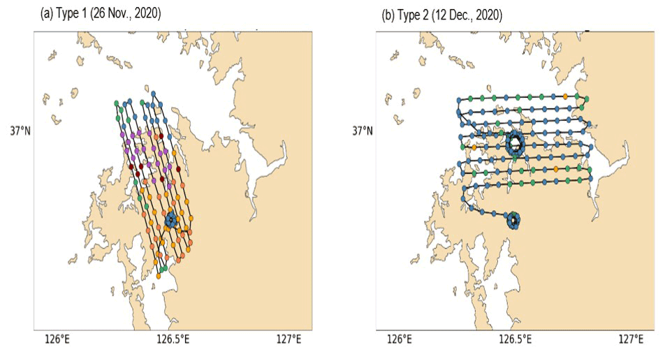
Figure 2Flight tracks for two Cessna Grand Caravan 208 B aircraft over Pandora sites (a) PA4 and (b) PA1 during the GMAP-2020 campaign. Colored circles indicate airborne NO2 concentration observations. Stacked circles indicate spiral flights conducted over two sites.
3.4 Meteorological measurements
Ground-based hourly observation data for meteorological variables were obtained from Seosan Automated Synoptic Observing System (ASOS) stations maintained by the KMA, and wind and temperature profile data were obtained twice daily (00:00 and 12:00 UTC) via a rawinsonde instrument at the Osan World Meteorological Organization upper air measurement station (47122) near Seosan. Due to time constraints of the sonde measurements, information on PBLH variation was obtained from Unified Model (UM) simulation results provided on the KMA website (https://afso.kma.go.kr, last access: 22 August 2022).
During the GMAP-2020 campaign, a 3D sonic anemometer (CPEC200; Campbell Scientific, Logan, UT, USA) was also installed on the rooftop at PA4 for turbulent flux measurements at the city–atmosphere interface (Hong et al., 2019). All wind components and sonic temperatures were measured at a 10 Hz sampling rate, and ground-level sensitive heat flux was measured directly using a 30 min averaging period. Quality controls such as double rotation, spike removal, and outlier filtering were also applied.
3.5 Correlation analyses
We examined the synergy of PC and SI data obtained during the GMAP-2020 campaign, and combined these measurement data to evaluate air quality in Seosan, South Korea. We attempted to interpret the meteorological and photochemistry data measured during GMAP-2020, and to demonstrate that caution is required when attempting to study the vertical structure of air pollutants using either surface observations or satellite data only, particularly in industrial areas.
First, we examined the combined use of year-long PC-NO2 and SI-NO2 measurements, and investigated the factors modulating their correlation. Numerous studies have examined the correlations between chemical species, including aerosols (Thomspon et al., 2019; Wang et al., 2019; Kim et al., 2012, 2018; Jo and Kim, 2013; Sanchez et al., 1990). Wang et al. (2019) reported that aerosols moderately correlate with NO2 due to the frequent occurrence of lifted layers probably related to the transport of pollutants. Jo and Kim (2013) differentiated haze types using the trajectory speed and direction and different synoptic conditions. In this background, we hypothesized that their differences in PC-NO2 and SI-NO2 were due to meteorological conditions, and performed k-means and agglomerative hierarchical cluster analyses of various meteorological variables. Clustering is the grouping of objects that are alike and are different from the objects belonging to other clusters. As a first step, k-means clustering was applied to find smaller clusters until each object was classified in one cluster. Subsequently, agglomerative hierarchical steps are applied to make up for the shortcomings of k-means clustering, in which once merging (or splitting) is done, it can never be undone. More details are found in Venkat Reddy et al. (2017). We used XLSTAT software (Addinsoft, Paris, France) for the cluster analysis with eight meteorological variables representing local and synoptic circulations in the cluster analysis: surface wind speed (Wsfc), 925 hPa temperature (T925), sea level pressure (Psfc), pressure tendency (), 850 hPa wind speed (W850) and its north–south and east–west components (NS850 and EW850), and 500 hPa geopotential height (GPH500). We subtracted 30 d moving averages from all data to account for typical seasonal variation. Monthly averages were used for PC-NO2 analysis due to the limited availability of hourly data.
Correlations between PC-NO2 and SI-NO2 were analyzed in each meteorological group and the impact of photochemistry was interpreted based on case-specific features. We also investigated correlations in association with near-surface micrometeorological variables such as PBLH in each meteorological group.
4.1 Correlation analysis results for PC-NO2 and SI-NO2
The yearly PC-NO2 statistics at four Pandora sites (PA1–PA4) are summarized in Table 1. The total averaged PC–NO2 over all sites was 0.45 DU during GMAP-2020, which is well above the typical values (0.1–0.2 DU) for Anmyeondo (the location is shown in Fig. 1), a representative background site (Herman et al., 2018). Although site PA3 is located in a rural area, it nevertheless exhibited the highest PC-NO2 amounts, suggesting that plumes were frequently transported from nearby point sources and/or urban areas.
Table 1Summary of NO2 column data from four Pandora (PA) measurement sites.
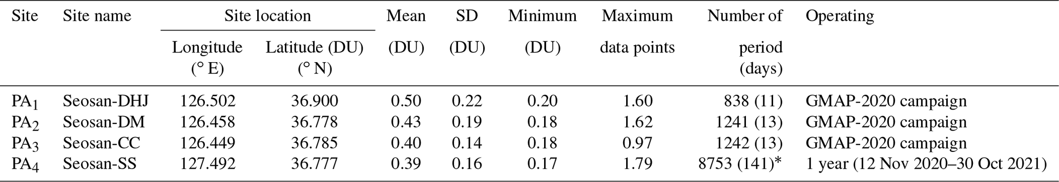
* The Pandonia Global Network (PGN) retrieval algorithm was applied to yearly measurements.
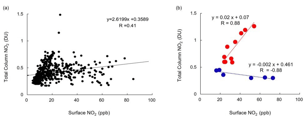
Figure 3(a) Pandora column (PC) NO2 measurements as a function of surface in situ (SI) NO2 observations at Pandora sites PA1–PA3 during the GMAP-2020 campaign and PA4 during a 1-year period. A 1:1 linear regression model was used to evaluate the relationship between PC and SI measurements (black line). (b) Sample scatterplots of PC-NO2 and SI-NO2 for 24 February (red) and 21 April 2021 (blue).
Scatter diagrams of hourly PC-NO2 and SI-NO2 measurements from Pandora sites PA1–PA3 (GMAP-2020) and PA4 (yearly measurement; 12 November 2020–30 October 2021) are shown in Fig. 3a. These hourly data had a fair 1:1 linear relationship (R=0.41), implying the overall uniformity of NO2 profiles, whereas the linear relationship with PC-NO2 weakened as SI-NO2 levels increased (Fig. 3a). It appears that the SI-NO2 has a distinct diurnal change despite the same PC-NO2, and higher variable surface NO2 levels may result from the relatively weaker linear relationship between PC-NO2 and SI-NO2. To explore these anti-correlation cases further, we selected the lower and upper bounds of the tendencies; these are plotted in Fig. 3b, which shows that PC-NO2 was positively correlated with SI-NO2 on 24 February 2021 (R=0.88), while a negative correlation occurred on 21 April 2021 (), indicating a wide range of case-specific correlations. The negative correlation on 21 April (Fig. 3b) implied that the nonhomogeneous NO2 distributions vertically were partially due to the photochemical process. For example, the decrease in PC-NO2 despite an increase in SI-NO2 might have occurred because NO2 is removed by photochemical loss; it can occur more severely in the upper atmosphere with high OH concentrations. Another possible reason is the occurrence of lifted layers related to pollutant transport, yielding sharp changes in vertical concentration from the surface to the upper layer. The case-specific discussion follows.
4.2 Impacts of meteorological conditions on correlations between PC-NO2 and SI-NO2
Our k-means cluster analysis distinguished three groups with the lowest within-group variance and largest among-group variance. Among the total of 141 cases, 47, 66, and 28 were classified into groups 1–3, respectively. Thus, group 2 had the largest proportion of cases (47 %) and group 3 had the smallest (20 %). The combination of meteorological components in group 1 indicated the end of a high-pressure system (Psfc > 0, ), with southerly winds (NS850 > 0) bringing warmer air (T925 > 0) to the region, leading to stable atmospheric stratification and weak surface winds (Fig. 4). This group 1 meteorological mode appeared to result in very weak NO2 ventilation, which produced the highest PC-NO2 and SI-NO2 values. Group 3 showed the opposite trend, with strong northerly winds bringing colder air into the region, leading to an unstable atmosphere and stronger surface winds, and ultimately decreasing PC-NO2 and SI-NO2 to their lowest levels.
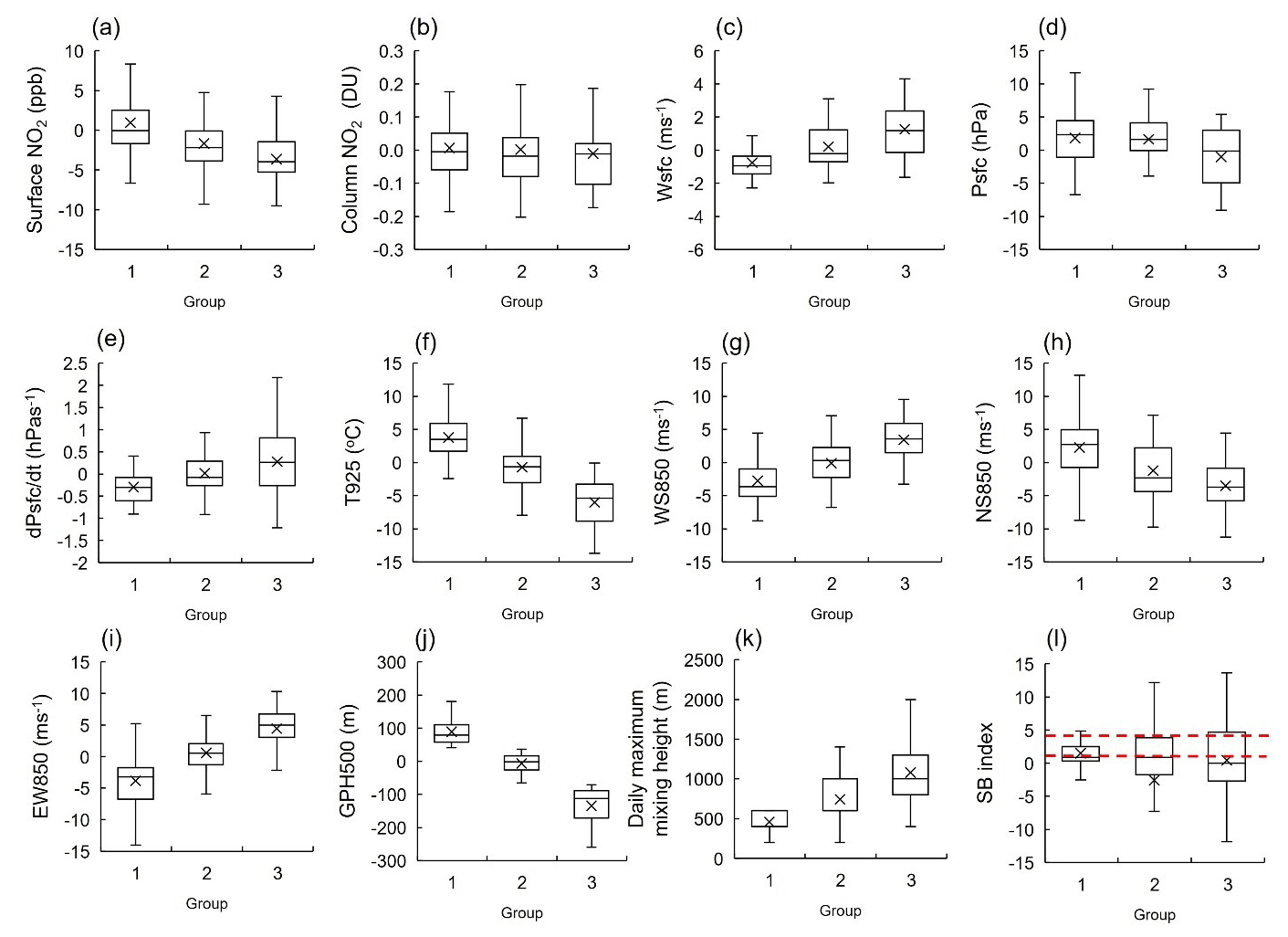
Figure 4K-means clustering yielded three groups of cases for (a) surface NO2 and (b) PC-NO2, associated with eight meteorological variables: (c) surface wind speed (Wsfc), (d) Psfc, (e) Psfc tendency (), (f) 925 hPa air temperature (T925), (g) 850 hPa wind speed (W850), (h) 850 hPa north–south wind component (NS850), (i) 850 hPa east–west wind component (EW850), and (j) 500 hPa geopotential height (GPH500). All data were de-seasonalized using the 30 d moving average, except PC-NO2, for which the monthly average was used. (k) Simulated daily maximum mixing height (not directly clustered). (l) Box and whisker plots of the sea breeze index (SBI) at Seosan for the 1-year period. Red dots indicate the critical SBI (a value of 3), suggested by Biggs and Graves (1962).
SI-NO2 was approximately twice as high in group 1 than group 3, whereas PC-NO2 showed no significant difference (Fig. 4a). We hypothesized that PBLH might also differ significantly under these micrometeorological conditions; therefore, we further explored daily maximum PBLH simulated by the Global Forecast System (GFS) and Lagrangian backward trajectories obtained from Hybrid Single-Particle Lagrangian Integrated Trajectory (HYSPLIT) and GFS system for the 141 cases. The mean simulated PBLH in Seosan, our study area, was 942.1±405.3 m for 2020, which was similar to the annual mean daily maximum PBLH (1013.6 m) in Osan (Lee et al., 2013). However, the simulated PBLH differed significantly among the three groups (767.0±304.8, 923.2±335.3, and 1280.6±501.2 m for groups 1–3, respectively). The PBLH for group 3 was 1.7-fold higher than that for group 1 (Fig. 4k). We also detected significant differences among the three groups in synoptic components of the lower troposphere including W850, and in local meteorological parameters such as the sea breeze index (SBI) suggested by Biggs and Graves (1962), which is defined as, , where U is Wsfc (Fig. 4c), Cp is specific heat, and ΔT is the temperature difference between T925 and the sea surface temperature. Thus, the SBI represents the ratio between inertial () and buoyance forces (ρgcpΔT), where ρ is air density and g is gravity, and its value provides an indication of the likelihood of local circulation events such as sea breezes; at higher SBIs (i.e., SBI > 3), sea breezes cannot overcome the prevailing wind, whereas lower SBIs (i.e., 0 < SBI < 3) can indicate strong sea breezes.
In the example shown in Fig. 4l, the SBI for groups 1–3 was 0.1±4.5, 0.1±9.2, and , respectively. Most SBIs in group 1 ranged from 0 to 3, indicating that group 1 corresponded to the dominant local circulation (LD), whereas the SBIs in group 3 had the lowest frequencies comparing 1 and 3, which corresponded to a dominant synoptic-scale circulation (SD). Group 2 can be considered a mixture of local and synoptic-scale circulation (MD). These results indicate that Seosan may experience frequent LD conditions (with sun on of the days of the year), with infrequent SD conditions ( of all days).
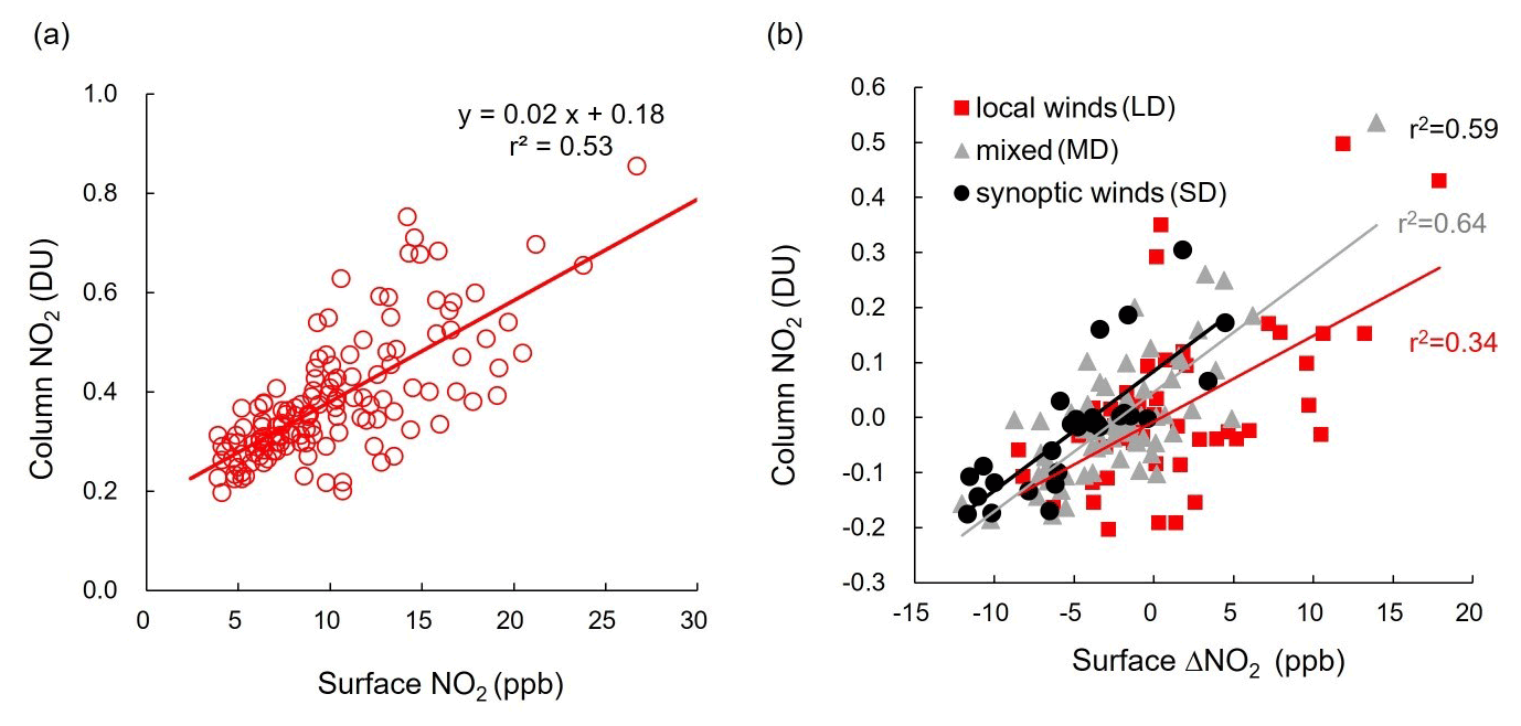
Figure 5(a) Scatterplots of daytime measurements at site PA4 (a) PC-NO2 vs. SI-NO2 under all meteorological conditions and (b) PC-NO2 vs. surface NO2 in each meteorological condition over a 1-year period (12 November 2020–30 October 2021). Here surface NO2 = SI-NO2 − (30 d moving average) SI-NO2.
4.2.1 Relationship between daily mean PC-NO2 and SI-NO2 under LD, MD, and SD conditions
Scatter diagrams of daytime mean PC-NO2 and SI-NO2 measurements at Seosan over the entire 1-year period are shown in Fig. 5. Based on the 141 cases, daytime mean values averaged between 11:00 and 17:00 KST were used to reduce the effect of nocturnal PBLH variation. Other data selection criteria included concurrent PC-NO2 and SI-NO2 measurements, with data acquisition rates of >80 % per day. Overall, PC-NO2 and SI-NO2 were strongly correlated (R=0.73; Fig. 5), suggesting that the vertical profiles were generally uniform in the PBL throughout all four seasons. The slope of the linear regression curve shown in Fig. 5a was 0.02 DU ppb−1 ( molec. cm−2 ppb−1), which is comparable to values (0.3–0.59×10¹⁵ molec. cm−2 ppb−1) obtained previously in a study of surface and OMI-NO2 measurements downwind of strong point sources in Israeli cities (Boersma et al., 2009). The intercept (0.17 DU) was within the range of previous Anmyeondo Pandora measurements, suggesting that intercepts of 0.15–0.2 DU may represent the local background PC-NO2 amount (including the stratospheric NO2), rather than the influence of local anthropogenic NO2 emissions.
We classified daily averaged PC-NO2 and SI-NO2 data according to the three meteorological conditions (LD, MD, and SD) and detected a weak correlation under LD conditions (Fig. 5b); the lowest coefficient of determination for the LD condition (R2=0.34) was approximately half of those for the MD (0.359) and SD (0.64) conditions, suggesting that NO2 vertical profiles were more complex under LD conditions, with anomalous layers.
4.2.2 Diurnal variation in column-surface NO2 under LD, MD, and SD conditions
Diurnal patterns of PC-NO2, SI-NO2, and O3 under SD, MD, and LD conditions are shown in Fig. 6. Under LD conditions, PC-NO2 increased from morning to afternoon (Fig. 6a), whereas under SD conditions, it had a weak morning peak and subsequent decrease until late afternoon (Fig. 6c). Under MD conditions, PC-NO2 had one large peak in the morning and a shoulder peak in the late afternoon (Fig. 6b). However, SI-NO2 showed nearly identical diurnal patterns among the three meteorological conditions, with an early morning peak followed by a second peak in the late afternoon (Fig. 6d–f). Diurnal patterns of O3 were strongly associated with O3-NO2 photochemical reactions under both LD and MD conditions (Fig. 6g and h), whereas no particular photochemical effects were detected under SD conditions (Fig. 6i).
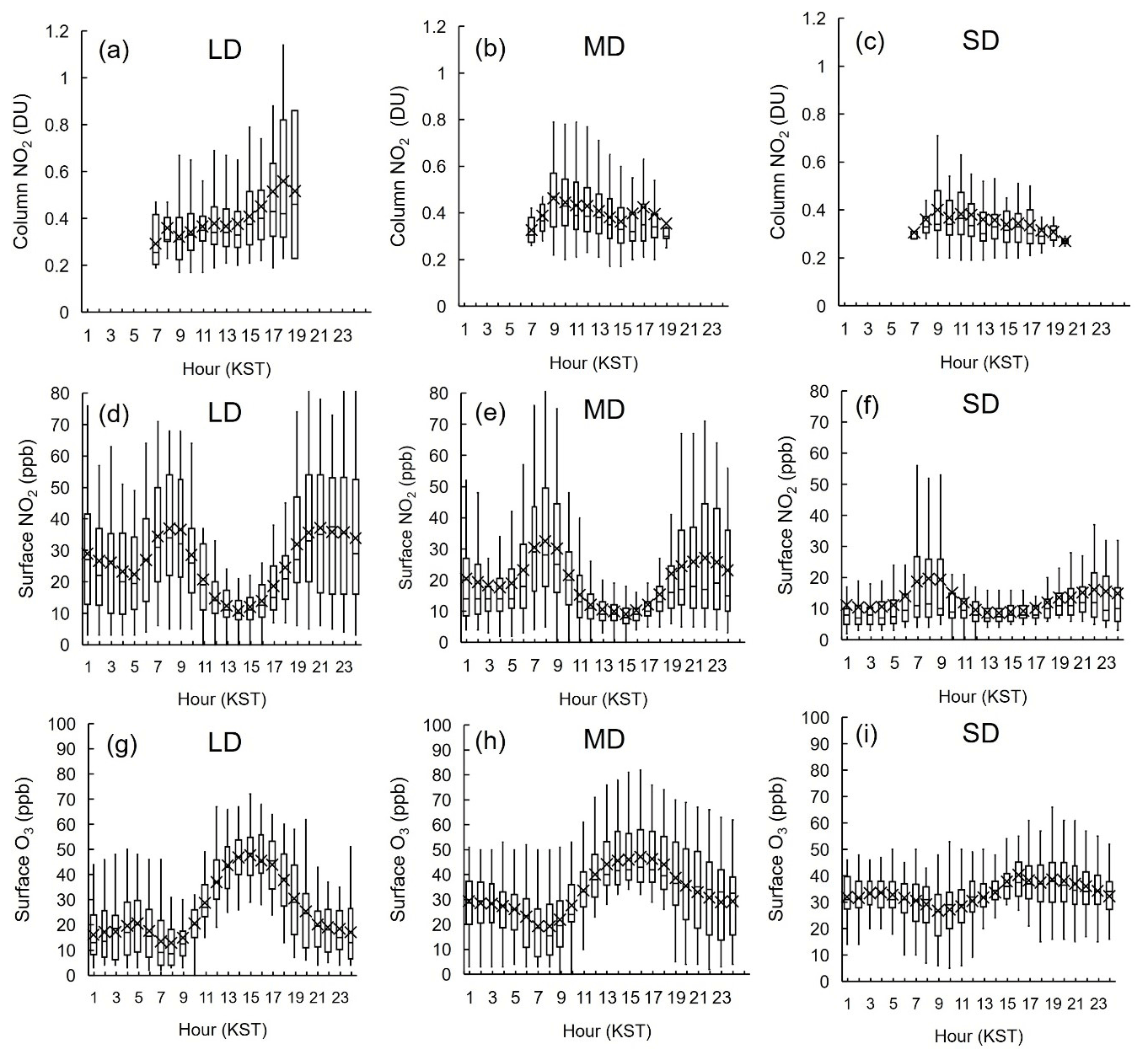
Figure 6Box and whisker plots of diurnal variation in (a–c) PC-NO2, (d–f) SI-NO2, and (g–i) surface O3 under synoptic wind-dominant (SD), mixed (MD), and local wind-dominant (LD) conditions in Seosan during a 1-year period (12 November 2020–30 October 2021).
A simple linear regression was applied to daytime average (11:00–17:00 LST) measurements of both PC-NO2 and SI-NO2 under the three meteorological conditions, and yielded correlation coefficients (R) of 0.51 and 0.41 for SD and MD conditions, respectively; however, LD conditions produced a significantly lower R (0.27). Thus, under SD conditions, strong synoptic winds suppressed PC-NO2 and SI-NO2 diurnal fluctuations, rendering them similar to each other. Strong winds also inhibited local effects of O3 formation on the diurnal variation in PC-NO2, and the smaller impact of chemical conversion from local NO2 to O3 lowered R values during the day. Under MD conditions, both PC-NO2 and SI-NO2 exhibited distinctive peaks in the morning with a degree of time lag; both subsequently declined toward noon, and showed higher R values than those obtained under SD conditions. By contrast, under MD conditions, correlations were enhanced due to a minimum around 15:00 KST for both PC-NO2 and SI-NO2, despite time lags in both peaks in the morning and afternoon.
Previous studies of the Megacity Air Pollution Seoul (MAPS-Seoul) and KORUS-AQ campaigns reported a typical pattern of continuously increasing PC-NO2 over the Seoul metropolitan area (Chong et al., 2018; Herman et al., 2018). However, in the current campaign, we found similar results only under LD conditions. The diurnal patterns reported in previous studies were mainly caused by the dominance of NO2 emissions sources over NO2 losses (Chong et al., 2018; Herman et al., 2018) among several processes associated with NO2 photochemical loss, including transport and deposition, which were also investigated in specific cases in the current study.
In this study, we extended the correlation analysis and investigated the correlation between hourly PC-NO2 and SI-NO2 data. The results show a lower correlation in the morning and a higher correlation in the afternoon (Fig. S1 in the Supplement). The respective median correlation coefficients for the LD, MD, and SD meteorological conditions were −0.71, 0.18, and 0.22 in the morning (09:00–12:00 LST), and 0.84, 0.77, and 0.79 in the afternoon (12:00–14:00 LST). These values may reflect PBL development. SI-NO2 decreases in the morning due to the rapid growth of the PBL, while PC-NO2 increases due to the accumulation of NO2 in the atmosphere, deriving a lower correlation. However, there is very little change in the PBL in the afternoon, and PC-NO2 and SI-NO2 show similar changes, yielding a positive correlation between them during the GMAP-2020 campaign.

Figure 7Box and whisker plots of the vertical NO2 and O3 profiles measured by GMAP aircraft superposed with in situ AQMS1 measurements during flights (a, b) FL-5 (6 December) and (d, e) FL-7 (6 and 9 December). Blue dashed lines are linear regression lines fitted to NO2 and O3 profiles within the planetary boundary layer (PBL). Black arrows indicate the simulated PBL height (PBLH) obtained from the Korea Meteorological Administration (KMA). HYSPLIT 24 h backward trajectories in Seosan are shown at altitudes of 100, 500, and 1000 m, starting at 16:00 KST on 26 November and 12:00 KST on 12 December.
4.3 Aircraft measurements collected during GMAP-2020
Data collected via aircraft during GMAP-2020 are summarized in Table 2. A total of nine aircraft measurements were conducted during the campaign period (12 November 2020–20 January 2021). Four of nine flights were conducted under LD conditions, and the remaining flights (except that on 27 November 2020) were conducted under MD conditions. No aircraft measurements were consistent with SD conditions during the GMAP-2020 campaign.
Table 2Summary of aircraft measurements collected during the Geostationary Environment Monitoring Spectrometer (GEMS) Map of Air Pollution (GMAP)-2020 campaign period (12 November 2020–20 January 2021).
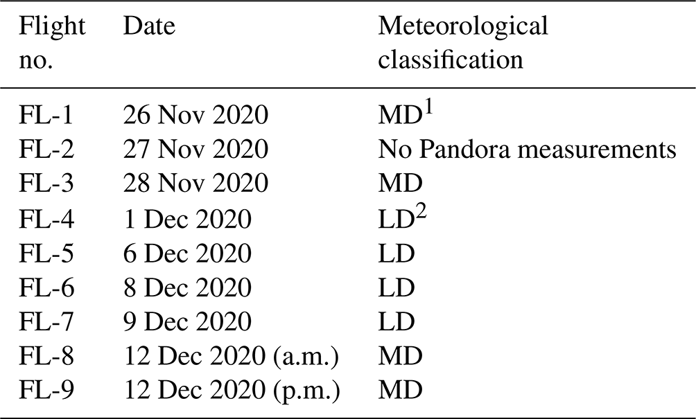
1 LD: local wind-dominant conditions; 2 MD: mixed conditions.
We examined spiral segments from each flight over Seosan during 11:00–17:00 KST to exclude marginal effects of diurnal variation in NO2 (Fig. 2). The overall results indicated that the vertical O3 profiles were relatively constant in the PBL, whereas NO2 profiles appeared to be highly dependent on meteorological conditions. We compared data collected during flights conducted under LD (one flight) and MD conditions (two flights) during the GMAP-2020 campaign, to examine differences in the vertical structures of the PA and SI observations.
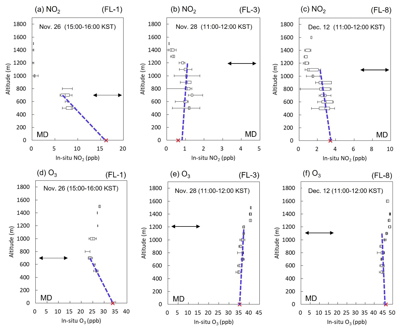
Figure 8Box and whisker plots of vertical profiles obtained from GMAP aircraft superposed with in situ AQMS measurements for (1) NO2 and (2) O3 for flights (a) FL-1 (26 November), (b) FL-3 (28 November), and (c) FL-8 (12 December). Blue dashed lines are linear regression lines fitted to NO2 and O3 in the PBL. Black arrows indicate PBLH simulated by the Hybrid Single-Particle Lagrangian Integrated Trajectory (HYSPLIT) Global Forecast System (GFS).
Aircraft measurements of vertical NO2 and O3 profiles for flights FL-5 (6 December) and FL-6 (8 December) under LD conditions are shown in Fig. 7, along with 24 h backward trajectories starting at different altitudes (100, 500, and 1000 m). All observed NO2 profiles shown in Fig. 7 appeared to have generally exponential curves, with anomalous features at higher altitudes. For example, when vertical turbulent mixing prevailed within the PBL (O3 profile, Fig. 7b), the data were fitted with an exponential vertical curve, and the anomalous NO2 layer aloft was found to have a height of 1.5 km, which was higher than the estimated PBLH of 1.2 km. HYSPLIT 24 h backward trajectories starting at 12:00 KST showed that all air mass from the surface to the lower free atmosphere was transported over the Yellow Sea via the Shandong Peninsula (Fig. 7c). This finding suggests that the anomalous NO2 layer aloft was not produced locally (i.e., from local LPS emissions), but instead traveled via long-range regional-scale transport. This transport of NO2 across the region was also discussed and might be particularly high during the winter when the NOx lifetime is relatively longer (Stohl et al., 2002; Wenig et al., 2003; Lee et al., 2013). According to Anmyeondo lidar measurements for 6 December (http://kalion.kr, last access: 22 August 2022), the anomalous NO2 layer aloft corresponded well to an aerosol layer that appeared at ∼1.0 km at approximately 12:00 KST, persisting until 2200 KST. However, based on a cross-comparison of our data, high surface levels of SI-NO2 ( ppb; Fig. 7a) were influenced more by local LPS than by that in the atmosphere aloft due to long-range transport (Fig. 7a).
Aircraft measurements for flight FL-7 (9 December) under LD conditions are shown in Fig. 7b. The NO2 vertical profile exhibited an exponential curve, with an anomalous peak at ∼600 m immediately above the top of the simulated PBL. HYSPLIT backward trajectory data starting at 12:00 KST showed that the non-surface air had a different origin from the surface air (Fig. 6d), indicating that the anomalous NO2 plume likely traveled from coal-fired power plants in a nearby industrial city (Taean) northwest of Seosan. This finding indicates a distinct vertical structure of higher NO2 at the surface due to strong local emissions, whereas lower NO2 levels were observed at higher altitudes, with anomalously high NO2 levels in some layers aloft due to medium-range transport from nearby areas. Thus, despite the limited number of aircraft measurements, the elevated anomalous NO2 structure that was observed intermittently led to a negative correlation between PA-NO2 and SI-NO2. The discrepancies imply that vertical profile distribution study should proceed cautiously when only surface measurements are obtained under LD meteorological conditions.
Aircraft measurements were conducted under MD conditions on flights FL-1 (26 November), FL-3 (28 November), and FL-8 (12 December) (Fig. 8). We applied several regression models (linear, exponential, and polynomial) to three vertical structures, and obtained two distinct NO2 vertical profile patterns from the surface to the PBLH: decreasing linearly for FL-1 and FL-8 (Fig. 8), and constant with altitude for FL-3 (Fig. 8b). None of the three cases showed anomalous layers above the PBLH, similar to the exponentially declining profiles obtained under LD conditions (Fig. 7). These vertical structures observed under MD conditions may have been induced by strong vertical mixing within the PBL, supplemented by prominent surface photochemical losses at the same time. The vertical O3 profile during FL-1 showed a decoupled structure, with different patterns within and above the PBL (Fig. 8d); however, the other 2 d showed uniform distributions, with no particular anomalous features between the upper PBL and surface atmosphere (Fig. 8b, c, e, and f). The observed daily maximum sensible heat fluxes measured at Seosan (Fig. S3) were much higher for FL-3 (175.9 W m−2) than FL-1 and FL-8 (118.9 and 102.0 W m−2), suggesting that vertical turbulent mixing was much more prominent during FL-3. These chemical and physical characteristics are all related to MD conditions. Thus, the higher coefficient of determination (R2=0.64) obtained under MD conditions (Fig. 5b) has an important bearing on the absence of irregular or anomalous layers aloft, with little variation regardless of the shape of the curve (Figs. 7 and 8).
4.4 Analyses of column–surface relationships for specific GMAP-2020 cases
Figure 9 shows examples of PC-NO2 and SI-NO2 diurnal variation under LD (FL-5 and FL-7) and MD (FL-1 and FL-8) conditions, and Fig. 10 shows latitudinal mean distributions for FL-5 and FL-7, based on the aircraft measurement data shown in Figs. 7 and 8. PC-NO2 was decoupled from SI-NO2 on 2 d, FL-5 and FL-7, which were both classified as having LD conditions (Fig. 9a and b), whereas good vertical mixing and uniform NO2 distribution were observed on the remaining 2 d, FL-1 and FL-8, which showed MD conditions (Fig. 9c and d). According to our analysis of the aircraft measurements (Fig. 7), the poor correlations between PC-NO2 and SI-NO2 captured by FL-5 and FL-7 were mainly due to an NO2 polluted layer transported aloft, as described in Sect. 4.3.
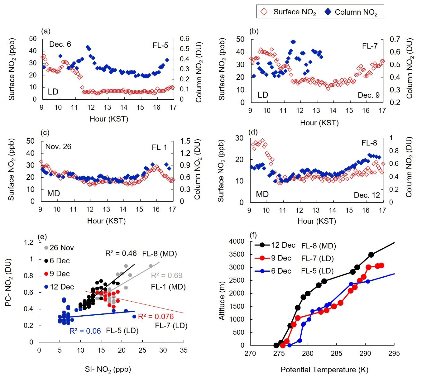
Figure 9Time series and scatterplots of PC-NO2 and SI-NO2 at PA2 on (a) 6 December, (b) 9 December, (c) 26 November, and (d) 12 December. (e) Scatterplot of PC-NO2 and SI-NO2 on 6 December (blue), 9 December (red), 26 November (gray), and 12 December (black). (f) Vertical potential temperature profiles on 6, 9, and 12 December 2020. Radiosonde data for 26 November 2020 are missing.
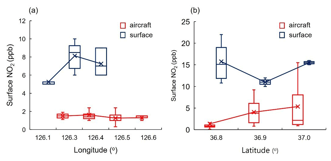
Figure 10Latitudinal NO2 distribution at the surface and 600 m over PA4 (Seosan super site), averaged during (a) 13:00–16:00 KST on 6 December (FL-5) by longitude and (b) 12:00–14:00 KST on 9 December (FL-7) by latitude, obtained from airborne (blue) and surface measurements (red).
4.4.1 LD conditions
Several cases showed poor correlations between PC-NO2 and SI-NO2 under LD conditions within the study period. When we examined the results of previous studies (Thompson et al., 2019; Chong et al., 2018; Herman et al., 2018; Kim et al., 2021), we first considered the possibility that LPS emissions influenced downwind regions under LD conditions because the increase in PC-NO2, but not SI-NO2, may have required an additional source of NO2 apart from early afternoon traffic emissions. The FL-5 data for December 6 represent an example of this, showing a poor correlation between PC-NO2 and SI-NO2 (R2=0.06; Fig. 9a). On the same day, Anmyeondo lidar detected two elevated aerosol layers at 12:00 and 16:00–22:00 KST (http://kalion.kr, last access: 22 August 2022); the first aerosol layer may reflect a PC-NO2 peak, as shown in Fig. 9a. The HYSPLIT backward trajectories, starting at different altitudes from the surface to the lower troposphere, revealed that all air parcels moved eastward from China to Anmyeondo and Seosan (Fig. 1); thus, other NO2 plumes may have begun to pass over Seosan at 16:00 KST (Fig. 7c). Longitudinal SI-NO2 distributions (Fig. 10) exhibited 5.2 ppb at 126.1∘ E, 8.1 ppb at 126.3∘ E, and 7.3 ppb at 126.4∘ E, averaged between 13:00 and 16:00 KST by longitude (Table S1 in the Supplement), whereas they were nearly constant at a height of 500–600 m on 6 December. Therefore, westerly winds advected cleaner air from Padori (AQM1) to Seosan at the surface, but not at a height of 500–600 m, contributing to low SI-NO2 levels in the afternoon (Fig. 9a).
Another example of a weak correlation was obtained by flight FL-7 (9 December), as shown in Fig. 9b. Time series PC-NO2 data exhibited several peaks during 12:00–14:00 KST (Fig. 9b), whereas SI-NO2 showed less temporal variation, resulting in a weak correlation () compared to the overall daytime (11:00–17:00 KST) correlation (R2=0.53; Fig. 5a). Latitudinal NO2 levels at high altitudes of ∼600 m (Fig. 10b) gradually increased northward, whereas surface NO2 was minimal at the midpoint. For example, at high altitudes, the latitudinal mean NO2 levels were 1.4 ppb (36.8∘ N), 4.1 ppb (36.9∘ N), and 5.1 ppb (37.0∘ N), whereas the SI-NO2 levels at the same sites were 18.0 ppb (36.8∘ N), 14.3 ppb (36.9∘ N), and 16.8 ppb (37.0∘ N), respectively, averaged during 12:00–14:00 KST by latitude (Table S1). This finding is attributable to a prevailing north wind that transported NO2 southward at high altitudes, while simultaneously ventilating SI-NO2 toward outer Seosan, resulting in the development of several PC-NO2 peaks. By contrast, SI-NO2 decreased slowly (Figs. 9b and 10b).
4.4.2 MD and SD conditions
We obtained higher PC–SI correlation coefficients under MD and SD conditions than LD conditions (Figs. 5b, and 9c and d). Under MD and SD conditions, diurnal variation in PC-NO2 and SI-NO2 showed simultaneous declines from early morning until noon (Fig. 6). Notably, PC-NO2 showed a continuously decreasing trend, particularly during the morning hours, in the period of approximately 09:00–12:00 KST under both MD and SD conditions (Fig. 6b and c). These diurnal patterns of decreasing PC-NO2 in the study area were opposite to those reported in previous studies (Chong et al., 2018; Herman et al., 2018) that observed increasing PC-NO2 in large urban areas during the daytime, caused by higher NO2 emissions even during photochemical NO2 losses to form O3.
We hypothesized that decreasing PC-NO2 can occur due to photochemical loss and surface wind transport, which both intensify with increasing solar radiation in the morning. Photochemically, NO2 is converted into photochemical oxidants such as PAN, HNO3, and nitrate under sunlight, thereby disrupting the NOx–VOC–O3 cycle. Concurrently, Wsfc intensified due to thermal turbulence transport of NO2 emissions away from Seosan during the day. Thus, PC-NO2 decreases under MD conditions as a result of ventilation effects caused by stronger wind speeds. There are two possible mechanisms for this: sea breeze penetration (because the study area is adjacent to the northern coast of the Taean Peninsula; Fig. 1), and vigorous turbulent mixing (which leads to vertical mixing of surface NO2 during PBL growth; Sun et al., 2013). We investigated these factors in detail for specific cases.
Figure 11 shows the diurnal variation in selected meteorological and chemical variables measured under MD (25 November) and SD conditions (14 December). Under MD conditions (Fig. 11a–c), declines in PC-NO2 and SI-NO2 were observed toward noon. In particular, decreasing PC-NO2 was accompanied by increased Wsfc (Fig. 11b); therefore, we examined GMAP-2020 campaign measurements of sea breeze penetration. Figure S2a shows diurnal variation in observed air temperatures at site Met1 and measured sea surface temperatures at nearby site Met2 (37.14∘ N, 126.01∘ E), located 55 km from PA4. The thermal meteorological observations were used to calculate SBI (+0.37), which was greater than +3 (the threshold for sea breeze occurrence; Brigges and Graves, 1962). Sea breeze disturbances with a sharp decrease (increase) in temperature (humidity) were observed at site Met3 (Fig. S3b), which is located on the northern coastline of Taean Peninsula (Fig. 1). However, sea breezes did not progress inland at the Met1 Seosan Meteorological Automated Surface Observing System (ASOS) site, which is closer to the Pandora sites; sea breezes did not correlate with NO2 ventilation to offset its high emission.
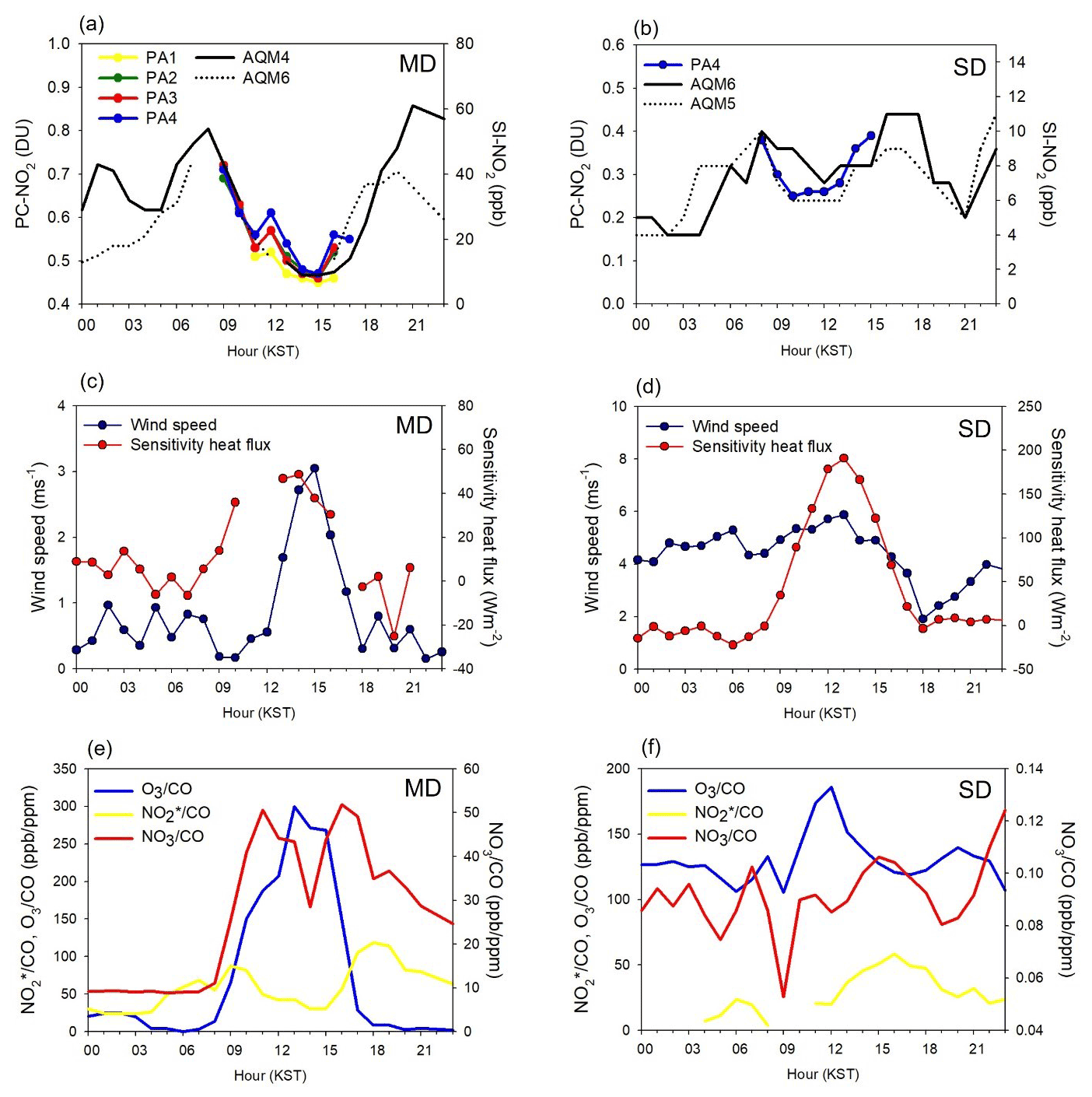
Figure 11Examples of the diurnal variation on 25 November (a, c, e) and 14 December (b, d, f). (a, b) Column NO2 at sites PA1–PA4, and surface NO2 at air quality monitoring sites AQM4 and AQM6. (c, d) Sensible heat fluxes and surface wind speed at PA4. (e, f) Diurnal variation in NO2, , and O3 normalized by CO. Figure 1 shows the locations of the measurement sites.
We further detected a strong positive correlation between wind speed and sensible heat flux (Fig. 11b). We speculated that thermal and momentum turbulences caused by a vertical temperature gradient and surface friction entrained surface turbulence, thus increasing momentum in the free atmosphere downward to the surface due to strong turbulent mixing within the PBL, in turn leading to a uniform vertical NO2 profile with a positive correlation between PC-NO2 and SI-NO2. Figure S3 shows a comparison of daily maximum sensible heat and momentum fluxes under LD, MD, and SD conditions during the GMAP-2020 campaign. SD conditions showed the highest mean heat flux, followed by MD and LD, indicating that downward momentum transport led by both heat and momentum fluxes plays a greater role in Wsfc enhancement under MD than LD conditions within the PBL.
Photolytic NO2 loss was detected as temporal variation in NO2, , and CO at PA4. Because no NO2 analyzer was installed at PA4, (= NOy–NO) was used instead of NO2 under the assumption that NOz is negligible in winter. Figure 11c shows the diurnal variation in NO2, O3, and under MD conditions, normalized by CO to reduce the effect of PBL evolution. The results showed that NO2/CO decreased after the morning peak; however, /CO and O3/CO increased toward midday, indicating that photolytic activity also contributed considerably to the concurrent decline of SI-NO2 and PC-NO2 (Fig. 11a). In turn, this indicated that photochemistry can contribute to higher correlation coefficients under MD conditions.
Under SD conditions (Fig. 11d–f), PA-NO2 and SI-NO2 exhibited weak diurnal variability compared to LD and MD conditions. SD conditions on 14 December produced significantly stronger winds (i.e., wind speed > 6 m s−1 at 13:00 KST), with generally higher PBLHs (Fig. 11e). Meteorological features, such as strong wind at both 850 hPa (18.0 m s−1) and 10 m height (4.26 m s−1), suppressed both PC-NO2 and SI-NO2 (7.3 ppb and 0.31 DU, respectively) to below the average, producing a strong correlation (R=0.9 at AQM5) and nearly flattening their temporal curves during the day (Fig. 11d). Thus, under SD conditions, wind speed and turbulent fluxes such as sensible heat flux had larger values, and NO2 and decreased or increased at the same time during the day (Fig. 11f), indicating that the transport effect was much greater than that of local photochemical loss over the study area.
In conclusion, in this case-specific study, we assessed the correlations between PC-NO2 and SI-NO2, and explored their mechanisms by investigating the impact of meteorological and photochemical conditions. A weak correlation between PC-NO2 and SI-NO2 occurred when anomalously high concentrations remained, with ragged fragments of NO2 plumes in the upper or middle layers. We also found that a negative correlation occurred intermittently under LD conditions, with generally lower PBLH. In particular, elevated pollutant levels due to regional-scale transport or decoupled NO2 plumes advected within the PBL may have also caused the weak correlation between PC-NO2 vs. SI-NO2. These phenomena were detected only from the PA–SI coupled measurements in this study. Thus, when either PC or SI observations are applied alone for understanding the vertical structure of air pollutants, undetected bias can occur under LD conditions, particularly where transport processes prevail, and these results can be also applicable to GEMS observations analysis.
We explored the potential applicability of combined PC-NO2 and SI-NO2 measurements collected at Seosan during the GMAP-2020 campaign. We characterized the correlation between PC-NO2 and SI-NO2 under various conditions to understand the complex air quality of Seosan, which appears to be vulnerable to LPS emissions from surrounding areas. We hypothesize that correlations between PC-NO2 and SI-NO2 are closely related to NO2 vertical profiles, which also depend on meteorological conditions. We performed statistical analyses of a year-long PC-NO2 dataset (12 November 2020–30 October 2021) combined with meteorological data, in situ ground data, and airborne chemical data measured during the GMAP-2020 campaign in the same period.
Our results show that hourly PC-NO2 and SI-NO2 over the 1-year period exhibited a linear relationship with a fair correlation (R=0.41), and daily mean PC-NO2 vs. SI-NO2 exhibited a good linear correlation (R=0.73), supporting the overall uniformity of NO2 profiles in the PBL over Seosan despite the continuous impact of LPS emissions.
The impact of meteorological conditions on the relationship between PC-NO2 and SI-NO2 was investigated through agglomerative hierarchical clustering, which indicated three meteorological conditions: LD, MD, and SD. Under LD conditions, southerly winds advect warm air under the upper ridge, forming stable and short PBLs and weak surface winds. By contrast, under SD conditions, cold northerly winds induce unstable and high PBLs with strong surface winds. The correlations between daily mean PC-NO2 and SI-NO2 levels, and their variation during 11:00–17:00 KST, weakened under LD conditions, suggesting that the shape of the NO2 profile typically deviates from a uniform profile under SD and MD conditions. Aircraft measurements under LD conditions demonstrated NO2 plumes aloft, with anomalous vertical structures and different horizontal (latitudinal) gradients of surface NO2 at higher altitudes, such as 600 m over Seosan.
Thus, the relationship between PC-NO2 and SI-NO2 depends on the presence of NO2 plumes aloft under LD conditions, which provide a favorable environment for LPS plumes decoupled from the surface at Seosan. Our findings suggest that the correlation between PC-NO2 and SI-NO2 may serve as an indicator of the degree of complexity of urban air quality. This correlation can be optimally applied for air quality evaluation and vertical analysis by combining the Pandora Asia Network with AQM networks, and the results can be also applied to environmental GEMS observation analysis in combination with SI observations. More detailed studies on urban air pollution evaluation will be undertaken based on PC, DOAS, aircraft, SI air quality, and surface turbulence observation data, as well as modeling studies of data collected during the GMAP-2021 campaign.
As a cluster analysis, k-means clustering and hierarchical analysis have been conducted using paid software code, XLSTAT software (https://www.xlstat.com/en/; Addinsoft, 2022), and a trial version of XLSTAT can be available at the same URL. All input data including Pandora measurement and surface measurements related to this paper are available from the corresponding author on reasonable request.
The measurements can be accessed by contacting the corresponding authors.
The supplement related to this article is available online at: https://doi.org/10.5194/acp-22-10703-2022-supplement.
LSC designed the research and managed the paper. DK, HH, DRK, JAY, KL, HL, DK, and JH conducted the experiments and provided data curation. HJY and DK contributed to formal analysis and visualization. CHK co-managed and substantially contributed to the discussion of the results.
The contact author has declared that none of the authors has any competing interests.
Publisher's note: Copernicus Publications remains neutral with regard to jurisdictional claims in published maps and institutional affiliations.
This article is part of the special issue “GEMS: first year in operation (AMT/ACP inter-journal SI)”. It is not associated with a conference.
We thank all those who contributed to the GMAP-2020 field campaign, NASA GSFC for use of Pandora instruments, and PGN for raw data processing.
This study was supported by the National Institute of Environmental Research (grant nos. NIER-2021-01-01-052 and NIER-2021-03-03-001), and was partially supported by National Research Foundation of Korea (NRF) funded by the Ministry of Education of the Republic of Korea (grant nos. 2020R1I1A2075417 and 2020R1A6A1A03044834).
This paper was edited by Chul Han Song and reviewed by two anonymous referees.
Addinsoft: The leading data analysis and statistical solution for Microsoft Excel®, Addinsoft Paris, France, https://www.xlstat.com/en/, last access: 22 August 2022.
Biggs, W. G. and Graves, M. E.: A lake breeze index, J. Appl. Meteorol., 1, 474–480, https://doi.org/10.1175/1520-0450(1962)001<0474:ALBI>2.0.CO;2, 1962.
Boersma, K. F., Jacob, D. J., Trainic, M., Rudich, Y., DeSmedt, I., Dirksen, R., and Eskes, H. J.: Validation of urban NO2 concentrations and their diurnal and seasonal variations observed from the SCIAMACHY and OMI sensors using in situ surface measurements in Israeli cities, Atmos. Chem. Phys., 9, 3867–3879, https://doi.org/10.5194/acp-9-3867-2009, 2009.
Cede A.: Manual for Blick Software Suite 1.7, Tech. rep., LuftBlick, Austria, 161 pp., https://www.pandonia-global-network.org/wp-content/uploads/2019/11/BlickSoftwareSuite_Manual_v1-7.pdf (last access: 22 August 2022), 2019.
Chong, H., Lee, H., Koo, J. H., Kim, J., Jeong, U., Kim, W., Kim, S. W., Herman, J. R., Abuhassan, N. K., Ahn, J. Y., Park, J. H., Kim, S. K., Moon, K. J., Choi, W. J., and Park, S. S.: Regional characteristics of NO2 column densities from Pandora observations during the MAPS-Seoul campaign, Aerosol Air Qual. Res. 18, 2207–2219, https://doi.org/10.4209/aaqr.2017.09.0341, 2018.
Engel-Cox, J. A., Holloman, C. H., Coutant, B. W., and Hoff, R. M.: Qualitative and quantitative evaluation of MODIS satellite sensor data for regional and urban scale air quality, Atmos. Environ., 38, 2495–2509, https://doi.org/10.1016/j.atmosenv.2004.01.039, 2004.
Flynn, C. M., Pickering, K. E., Crawford, J. H., Weinheimer, A. J., Diskin, G., Thornhill, K. L., Loughner, C., Lee, P., and Strode, S. A.: Variability of O3 and NO2 profile shapes during DISCover-AQ: Implications for satellite observations and comparisons to model-simulated profiles, Atmos. Environ., 147, 133–156, https://doi.org/10.1016/j.atmosenv.2016.09.068, 2016.
Herman, J., Cede, A., Spinei, E., Mount, G., Tzortziou, M., and Abuhassan, N.: NO2 column amounts from ground-based Pandora and MFDOAS spectrometers using the direct-sun DOAS technique: Intercomparisons and application to OMI validation, J. Geophys. Res.-Atmos., 114, D13307, https://doi.org/10.1029/2009JD011848, 2009.
Herman, J., Spinei, E., Fried, A., Kim, J., Kim, J., Kim, W., Cede, A., Abuhassan, N., and Rozenhaimer, S. M.: NO2 and HCHO measurements in Korea from 2012 to 2016 from Pandora spectrometer instruments compared with OMI retrievals and with aircraft measurements during the KORUS-AQ campaign, Atmos. Meas. Tech., 11, 4583–4603, https://doi.org/10.5194/amt-11-4583-2018, 2018.
Hong, J.-W., Lee, S.-D., Lee, K., and Hong, J.: Seasonal variations in the surface energy and CO2 flux over a high-rise, high-population, residential urban area in the East Asian monsoon region, Int. J. Climatol., 40, 4384–4407, https://doi.org/10.1002/joc.6463, 2019.
Jo, H.-Y. and Kim, C.-H: Identification of long-range transported haze phenomena and their meteorological features over Northeast Asia, J. Appl. Meteorol. Clim., 52, 1318–1328, https://doi.org/10.1175/JAMC-D-11-0235.1, 2013.
Kim, C.-H., Park, S.-Y., Kim, Y.-J., Chang, L.-S., Song, S.-K., Moon, Y.-S., and Song, C.-K.: A Numerical Study on Indicators of Long-range Transport Potential for Anthropogenic Particle Matter over Northeast Asia, Atmos. Environ., 58, 35–44, https://doi.org/10.1016/j.atmosenv.2011.11.002, 2012.
Kim, C.-H., Lee, H.-J., Kang, J.-E., Jo, H.-Y., Park, S.-Y., Jo, Y.-J., Lee, J.-J., Yang, G.-H., Park, T., and Lee, T.: Meteorological Overview and Signatures of Long-range Transport Processes during the MAPS-Seoul 2015 Campaign, Aerosol Air Qual. Res., 18, 2173–2184, https://doi.org/10.4209/aaqr.2017.10.0398, 2018.
Kim, J., Jeong, U., Ahn, M.-H., Park, R. J., Lee, H., Song, C. H., Choi, Y.-S., Lee. K.-H. Yoo, J.-M., Jeong, M.-J. Park, S. K., Lee, K.-M., Song, C.-K., Kim, S.-W., Kim, Y. J., Kim, S.-W., Kim, M., Go, S., Liu, X., Chance, K., Miller, C. C., Al-Saadi, J., Veihelmann, B., Bhartia, P. K., Torres, O., Abad, G. G., Haffner, D. P., Ko, D. H., Lee, S. H., Woo, J.-H., Chong, H., Park, S. S., Micks, D., Choi, W. J., Moon, K.-J., Veefkind, P., Levelt, P. F., Edwards, D. P., Kang, M., Eo, M., Bak, J., Baek, K., Kwon, H.-A., Yang, J., Park, J., Han, K. M., Kim, B.-R., Shin, H.-W., Choi, H., Lee, E., Chong, J., Cha, Y., Koo, J.-H., Hayashida, S., Kasai, Y., Kanaya, Y., Liu, C., Lin, J., Crawford, J. H., Carmichael, G. R., Newchurch, M. J., Lefer, B. L., Herman, J. R., Swap, R. J., Lau, A. K. H., Kurosu, T. P., Jaross, G., Ahlers, B., Dobber, M., McElroy, T. C., and Choi, Y.: New era of air quality monitoring from space: Geostationary Environment Monitoring Spectrometer (GEMS), B. Am. Meteorol. Soc., 101, E1–E22, https://doi.org/10.1175/BAMS-D-18-0013.1, 2020.
Kim, S.-M., Koo, J.-H., Lee, H., Mok, J., Choi, M., Go, S., Lee, S., Cho, Y., Hong, J., and Seo, S.: Comparison of PM2.5 in Seoul, Korea Estimated from the Various Ground-Based and Satellite AOD, Appl. Sci., 11, 10755, https://doi.org/10.3390/app112210755, 2021.
Kim, S.-U. and Kim, K.-Y.: Physical and chemical mechanisms of the daily-to-seasonal variation of PM10 in Korea, Sci. Total Environ., 712, 136429, https://doi.org/10.1016/j.scitotenv.2019.136429, 2020.
Lamsal, L. N., Martin, R. V., van Donkelaar, A., Celarier, E. A., Bucsela, E. J., Boersma, K. F., Dirksen, R., Luo, C., and Wang, Y.: Indirect validation of tropospheric nitrogen dioxide retrieved from the OMI satellite instrument: Insight into the seasonal variation of nitrogen oxides at northern midlatitudes, J. Geophys. Res., 115, D05302, https://doi.org/10.1029/2009JD013351, 2010.
Lee, S., Kim, M., Kim, S. Y., Lee, D. W., Lee, H., Kim, J., Le, S., and Liu, Y.: Assessment of long-range transboundary aerosols in Seoul, South Korea from Geostationary Ocean Color Imager (GOCI) and ground-based observations, Environ. Pollut., 269, 115924, https://doi.org/10.1016/j.envpol.2020.115924, 2021.
Lee, S. J., Lee, J., Greybush, S. J., Kang, M., and Kim, J.: Spatial and temporal variation in PBL height over the Korean Peninsula in the KMA operational regional model, Adv. Meteorol., 2013, 1–16, https://doi.org/10.1155/2013/381630, 2013.
NIER – National Institute of Environmental Research: Air Quality Monitoring Network Installation and Operation, Ministry of the Environment, Seoul, Korea, https://www.airkorea.or.kr/web/board/3/267/?page=2&pMENU_NO=145 (last access: 22 August 2022), 2021.
Sanchez, M. L., Pascual, D., Ramos, C. and Perez, I.: Forecasting particulate pollutant concentrations in a city from meteorological variables and regional weather patterns, Atmos. Environ, 6, 1509–1519, https://doi.org/10.1016/0960-1686(90)90060-Z, 1990.
Stohl, A., Eckhardt, S., Forster, C., James, P., and Spichtinger, N.: On the pathways and timescales of intercontinental air pollution transport, J. Geophys. Res., 107, 4684, https://doi.org/10.1029/2001JD001396, 2002.
Sun, J., Lenschow, D. H., Mahrt, L., and Nappo, C.: The relationships among wind, horizontal pressure gradient, and turbulent momentum transport during CASES-99, J. Atmos. Sci., 70, 3397–3414, https://doi.org/10.1175/JAS-D-12-0233.1, 2013.
Thompson, A. M., Stauffer, R. M., Boyle, T. P., Kollonige, D. E., Miyazaki, K., Tzortziou, M., Herman, J. R., Abuhassan, N., Jordan, C. E., and Lamb, B. T.: Comparison of near-surface NO2 pollution with Pandora total column NO2 during the Korea-United States Ocean Color (KORUS OC) Campaign, J. Geophys. Res.-Atmos.,124, 13560–13575, https://doi.org/10.1029/2019JD030765, 2019.
Van Roozendael, M. and Fayt, C.: WinDOAS Software user manual, Tech. rep., IASB/BIRA, Uccle, Belgium, http://uv-vis.aeronomie.be/software/WinDOAS (last access: 22 August 2022), 2001.
Venkat Reddy, M., Vivekananda, M., and Satish, R.: Divisive Hierarchical Clustering with K-means and Agglomerative Hierarchical Clustering, Int. J. Comput. Sci. Trends Tech., 5, 6–12, https://doi.org/10.17485/ijst/2016/v9is1/96012, 2017.
Wang, J. and Christopher, S. A.: Intercomparison between satellite-derived aerosol optical thickness and PM2.5 mass: Implications for air quality studies, Geophys. Res. Lett., 30, 2095, https://doi.org/10.1029/2003GL018174, 2003.
Wang, Y., Dörner, S., Donner, S., Böhnke, S., Smedt, I. D., Dickerson, R. R., Dong, Z., He, H., Li, Z., Li, D., Ren, X., Theys, N., Wang, Y., Wang, Z., Xu, H., Xu, J., and Wagner, T.: Vertical profiles of NO2, SO2, HONO, HCHO, CHOCHO and aerosols derived from MAX-DOAS measurements at a rural site in the central western North China Plain and their relation to emission sources and effects of regional transport, Atmos. Chem. Phys., 2, 5417–5449, https://doi.org/10.5194/acp-19-5417-2019, 2019.
Wenig, M., Spichtinger, N., Stohl, A., Held, G., Beirle, S., Wagner, T., Jähne, B., and Platt, U.: Intercontinental transport of nitrogen oxide pollution plumes, Atmos. Chem. Phys., 3, 387–393, https://doi.org/10.5194/acp-3-387-2003, 2003.
Zhao, X., Griffin, D., Fioletov, V., McLinden, C., Davies, J., Ogyu, A., Lee, S. C., Lupu, A., Moran, M. D., Cede, A., Tiefengraber, M., and Müller, M.: Retrieval of total column and surface NO2 from Pandora zenith-sky measurements, Atmos. Chem. Phys., 19, 10619–10642, https://doi.org/10.5194/acp-19-10619-2019, 2019.