Evaluation of the WRF and CHIMERE models for the simulation of PM_2.5 in large East African urban conurbations

Urban conurbations of East Africa are affected by harmful levels of air pollution. The paucity of local air quality networks and the absence of the capacity to forecast air quality make difficult to quantify the real level of air pollution in this area. The CHIMERE chemistry transport model has been used along with the Weather Research and Forecasting (WRF) meteorological model to run high-spatial-resolution (2 × 2 km) simulations of hourly concentrations of particulate matter with an aerodynamic diameter smaller than 2.5 µm (PM_2.5) for three East African urban conurbations: Addis Ababa in Ethiopia, Nairobi in Kenya, and Kampala in Uganda. Two existing emission inventories were combined to test the performance of CHIMERE as an air quality model for a target monthly period in 2017, and the results were compared against observed data from urban, roadside, and rural sites. The results show that the model is able to reproduce hourly and daily temporal variabilities in aerosol concentrations that are close to observed values from urban, roadside, and rural environments. CHIMERE's performance as a tool for managing air quality was also assessed. The analysis demonstrated that, despite the absence of high-resolution data and up-to-date biogenic and anthropogenic emissions, the model was able to reproduce 66 %–99 % of the daily PM_2.5 exceedances above the World Health Organization (WHO) 24 h mean PM_2.5 guideline (25 µg m⁻³) in the three cities. An analysis of the 24 h average PM_2.5 levels was also carried out for 17 constituencies in the vicinity of Nairobi. This showed that 47 % of the constituencies in the area exhibited a poor Air Quality Index for PM_2.5 that was in the unhealthy category for human health, thereby exposing between 10 000 and 30 000 people per square kilometre to harmful levels of air contamination.

1 Introduction

The world's population has grown rapidly by 1 billion people over the last 12 years, reaching 7.9 billion in 2021. The World Population Prospects (WPP) made by the United Nations (UN) suggest a continuing annual increase of 1.8 %, meaning that the global population will reach 8.5 billion by 2030, 9.7 billion by 2050, and 11.2 billion by 2100 (UNEP, 2019). The African continent is predicted to have the fastest growing population rate in the world, and it is projected to double between 2010 and 2050, surpassing 2 billion (UN-WPP, 2019). In addition to this, a 60 % increase in population has been predicted by 2050, specifically in urban areas (UN-WPP, 2019).

The populations in countries in sub-Saharan East Africa (SSEA) increased drastically from 1991 to 2019. During that period of time, according to data from the World Bank database (World Bank Open Data, 2022), the Kenyan population grew from 24 to 52 million, the Ugandan population grew from 17 to 44 million, and the Ethiopian population grew from 50 to 112 million. These increases in population were accompanied by a similar rate of increase in road transport, industrial activities, and in the use of solid fuels (e.g. woods, charcoal, and agricultural residues) for cooking purposes in urban areas (Bockarie et al., 2020; Marais et al., 2019).

As a result of these population increases, the air quality of urban areas in these countries, which has historically been influenced by the large presence of seasonal biomass burning emissions (Haywood et al., 2008; Lacaux, 1995; Liousse et al., 2010; Thompson et al., 2001), is progressively degrading (Marais and Wiedinmyer, 2016). This, in combination with the expanding urban population, has greatly increased the exposure of citizens to harmful particulate matter (PM) pollution with an aerodynamic diameter smaller than 10 (PM₁₀) and 2.5 µm (PM_2.5) (Gatari et al., 2019; Kinney et al., 2011; Li et al., 2017; UN-Habitat, 2017).

Several diseases have been attributed to PM exposure in SSEA, including cardiovascular and cardiopulmonary diseases, cancers, and respiratory deep infections (Dalal et al., 2011; Mbewu and Mbanya, 2006; Parkin et al., 2008). In 2012, the World Health Organization (WHO) estimated that 176 000 deaths in SSEA were directly connected to air pollution (WHO, 2012). Modelling studies have also found that exposure to outdoor air pollution has led to 626 000 disability-adjusted life years (DALYs) in SSEA alone (Amegah and Agyei-Mensah, 2017), highlighting that these numbers could be much higher considering the limited amount of air quality data emanating from the region that are available for research purposes.

Considering the likely severe impacts of air pollution on human health in SSEA, the research interest in understanding air pollution trends in East Africa has increased in recent years. Many researchers have analysed the levels of contamination using short-term measurement campaigns (Amegah and Agyei-Mensah, 2017; deSouza et al., 2017; Egondi et al., 2013; Gaita et al., 2014; Gatari et al., 2019; Kume, 2010; Ngo et al., 2015; Pope et al., 2018; Schwander et al., 2014; van Vliet and Kinney, 2007; Singh et al., 2021). Other studies have observed annual average PM_2.5 concentrations in the order of 100 µg m⁻³, quantified in a small number of urban areas, in SSEA (Brauer et al., 2012). These levels are about 4 times higher than the 24 h average and 10 times higher than the annual average WHO guideline values for PM_2.5 (Avis and Khaemba, 2018; WHO, 2016), and they underline that air pollution is a serious problem in this area of the world. A recent study by Singh et al. (2020), using visibility as a proxy for PM, showed that air quality in Addis Ababa, Kampala, and Nairobi has degraded alarmingly over the last 4 decades.

The lack of long-term air quality monitoring networks in many African countries has made it difficult to acquire reliable long-term air quality data (Petkova, 2013; Pope et al., 2018; Singh et al., 2020), and little is currently known about the levels of air contamination in the region's large urban conurbations (Burroughs Peña and Rollins, 2017). However, the paucity and sometimes complete absence of reliable data on air pollution levels make it difficult to quantify the magnitude of the problem. Consequently, it is difficult for local and national authorities to plan possible improvement measures for the mitigation of anthropogenic emissions. Even if important steps forward have been made to improve the knowledge available regarding anthropogenic emissions and the emission inventories for Africa used for numerical simulations and forecasts of air quality (Assamoi and Liousse, 2010; Liousse et al., 2014; Marais and Wiedinmyer, 2016), the lack of surface observations to validate the emission magnitude and the simulated concentrations make these inventories susceptible to large error.

In this work, we test a meteorological and a chemistry transport model (CTM) to simulate the hourly urban and rural levels of PM_2.5 in three SSEA urban conurbations during a monthly period in 2017. We present the validation results for both models for the capital cities of Kenya, (Nairobi), Ethiopia (Addis Ababa), and Uganda (Kampala) against observational data. For Nairobi, we compare model outputs with observations from rural and roadside site observations collected during the “A Systems approach to Air Pollution in East Africa” research project (ASAP-East Africa – https://www.asap.uk.com/ (last access: 14 May 2022), hereafter called ASAP) (Pope et al., 2018). For Addis Ababa and Kampala, the model was validated using hourly observations of PM_2.5 collected by the respective US embassies.

We also assess the suitability of the CTM as a decision support tool for policymakers to plan possible mitigation policies oriented to quantify the real level of air pollution in urban areas as well as the human exposure to PM_2.5. Specifically, in terms of the accuracy of the model, we estimate the daily WHO threshold limit exceedances of PM_2.5 in the three urban conurbations. Finally, for the particular case of Nairobi, we evaluate the average air quality indices by local constituency for the whole analysis period, giving new insight into the real level of air contamination in Nairobi and into the relative population exposed to harmful levels of air contamination.

2 Material and methods

The meteorological and chemistry transport models employed in this work have been configured to simulate hourly weather parameters and concentrations of PM_2.5 using available input data for the simulations and using observations from the real world for the validation. The observations for the validation of both models are available from different providers; therefore, they have different temporal frequencies and, in the case of PM_2.5 observations, come from different environments (rural, urban, and roadside sites). No vertical observations were available for the validation of both models.

2.1 The Weather Research and Forecasting (WRF) meteorological model

The Weather Research and Forecasting (WRF) model is a numerical model for weather predictions and atmospheric simulations that is used both commercially and for research purposes, including by the US National Oceanic and Atmospheric Administration (Powers et al., 2017; Skamarock et al., 2008).

WRF was employed to drive the meteorology for CHIMERE using three geographical domains at different resolutions (from 18 × 18 to 2 × 2 km) that were vertically divided into 30 levels, 9 of which were below 1500 m. The first external domain has an 18 × 18 km spatial resolution (Fig. 1), with three nested domains at a 6 × 6 km resolution centred on the three countries of interest (Fig. 1, white squares). Three further nested domains with a 2 × 2 km resolution centred on Addis Ababa, Kampala, and Nairobi (Fig. 1, white dashed squares; Fig. 2) are the focus of the analysis.

Figure 1 The spatial distribution of the PM_2.5 emissions from the DICE–EDGAR merged emission inventory for East Africa for the WRF domain at a 18 × 18 km resolution. The continuous white lines show the location of the first nested domain at a 6 × 6 km resolution used in WRF–CHIMERE. The dashed white squares give the locations of the second nested domains at a 2 × 2 km resolution centred on Addis Ababa (Ethiopia, white triangle), Kampala (Uganda, white square), and Nairobi (Kenya, white circle) used for WRF–CHIMERE.

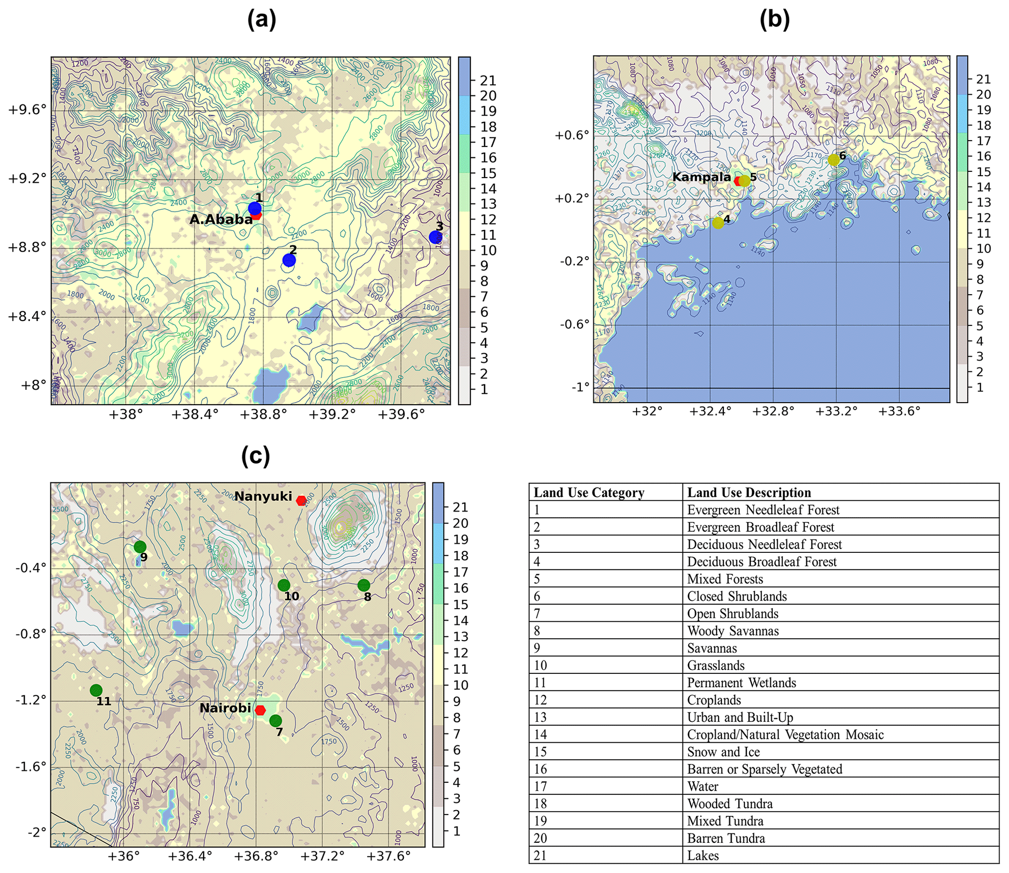
Figure 2 The second nested domains at a 2 × 2 km spatial resolution centred on the cities of (a) Addis Ababa (ETH2K), (b) Kampala (UGA2K), and (c) Nanyuki and Nairobi (KEN2K) created using the WRF model outputs. The red dots represent the locations of PM_2.5 measurements. The blue, yellow, and green dots refer to the location of the ground weather stations used for the meteorological validation in Ethiopia, Uganda, and Kenya respectively. The numbers relate to the stations detailed in Table 2. Contour lines are relative to the height (metres above ground level) from WRF outputs, and the colour scale applied to the maps in panels (a), (b), and (c) represents the 21 land use classification classes adopted in WRF simulations. The description of each land use category is provided the legend.

The configuration adopted for the WRF simulations has been chosen according to previous work focused on East Africa (Kerandi et al., 2016, 2017; Pohl et al., 2011) and is summarised in Table 1. The Yonsei University Scheme (YSU – Hong et al., 2006) was chosen to represent the planetary boundary layer while the Community Atmosphere Model (CAM – Collins et al., 2004) was used for the long- and short-wave radiation scheme. Initial and boundary conditions for the external coarse domain at 18 × 18 km were obtained from the National Centers for Environmental Prediction (NCEP) Final (FNL) Operational Global Analysis data (Wu et al., 2002). Boundary condition for the first (6 × 6 km) and second (2 × 2 km) nested domains were taken from the respective parent domains using a two-way nesting approach. This process enables the lateral conditions for the internal domains to be calculated from the outputs of the respective parent domains at lower resolution at every time step of the simulation.

Table 1 Main configuration parameters adopted for the WRF–CHIMERE modelling system for all simulations.

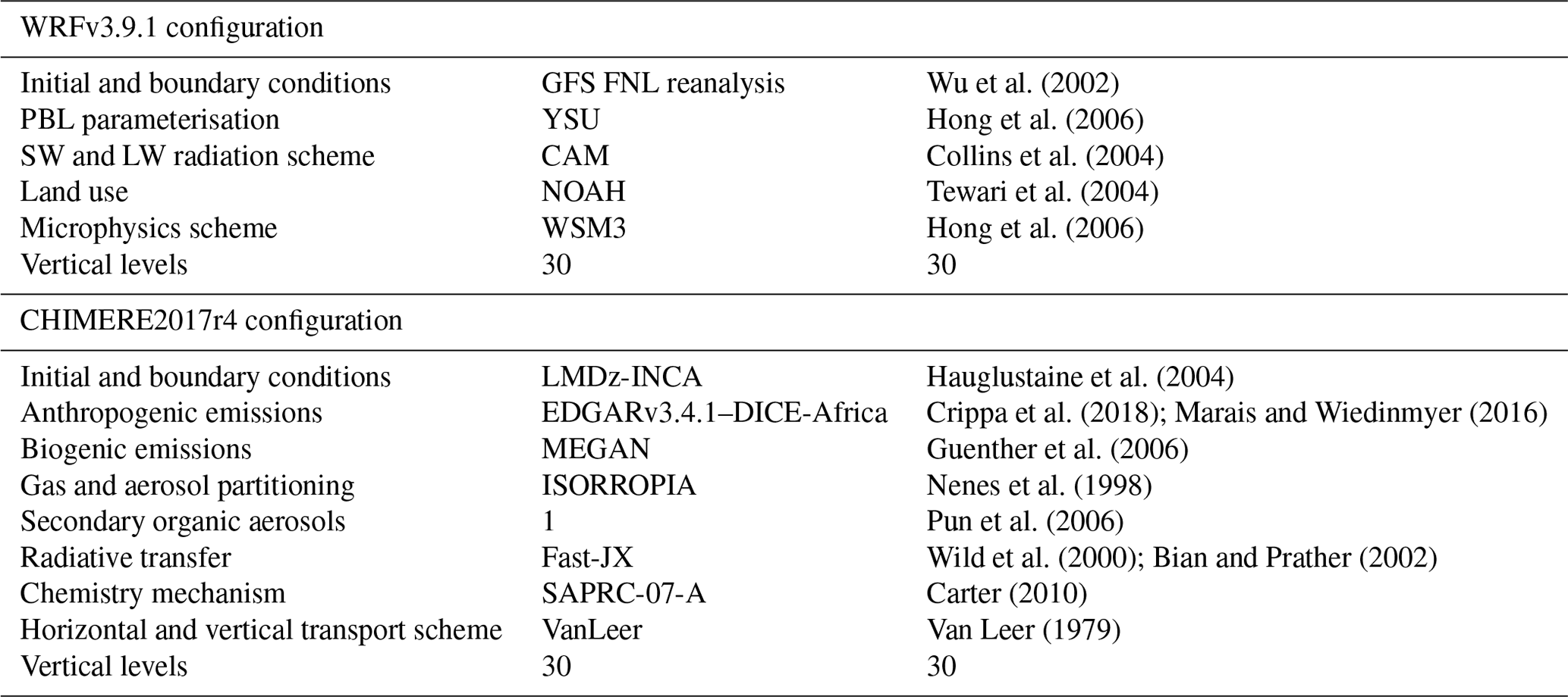
The abbreviations used in the configuration column in the table are as follows: PBL – planetary boundary later, SW – short-wave, and LW – long-wave.

The land use option chosen for the simulations was NOAH (Tewari et al., 2004), while the WRF single–moment 3–class scheme (WSM3) for clouds and ice proposed by Hong et al. (2004) was chosen for the reproduction of the microphysical processes in WRF.

2.2 The CHIMERE chemistry transport model

CHIMERE, version 2017r4 (Mailler et al., 2017), is an Eulerian numerical model for reproducing three-dimensional gas-phase chemistry and aerosol processes of formation, dispersion, and wet and dry deposition over a defined domain with flexible spatial resolutions. CHIMERE has been used for a number of comparative research studies of ozone and PM₁₀ from the continental scale, (Bessagnet et al., 2016; Zyryanov et al., 2012) to the urban scale (van Loon et al., 2007; Vautard et al., 2007; Mazzeo et al., 2018). Furthermore, the model has been used for event analysis, scenario studies (Markakis et al., 2015; Trewhela et al., 2019), forecasts, and impact studies of the effects of air pollution on health (Valari and Menut, 2010) and vegetation (Anav et al., 2011). The authors highlight that version 2017r4 of CHIMERE is adopted in this study, which was the most recent version available at the time that the present work was realised.

The CHIMERE model has been used to simulate the first nested domains at a 6 × 6 km spatial resolution and the second nested domains at a 2 × 2 km spatial resolution. The configuration adopted in this work uses initial and boundary conditions from the LMDz-INCA global three-dimensional chemistry transport model (Hauglustaine et al., 2004), for both gaseous pollutants and aerosols, for the most external domain at a 6 × 6 km resolution, whereas the boundary conditions are calculated from model outputs of the parent domains for the most internal domains at a 2 × 2 km resolution. The complete chemical mechanism used for all of the simulations was SAPRC-07-A (Carter, 2010), which can describe more than 275 reactions of 85 species. SAPRC-07-A is the most recent chemical mechanism available for CHIMERE version 2017r4.

Horizontal and vertical diffusion is calculated using the approach suggested by Van Leer (1979), and the ISORROPIA thermodynamic equilibrium model (Nenes et al., 1998) is used for the particle and gas partitioning of semi-volatile inorganic gases. The model permits the calculation of the thermodynamical equilibrium between sulfates, nitrates, ammonium, sodium, chloride, and water depending upon temperature and relative humidity data.

Dry deposition and wet deposition are calculated in CHIMERE. The particle dry-deposition velocities are calculated as a function of particle size and density as well as relevant meteorological variables, including deposition processes, such as turbulent transfer, Brownian diffusion, impaction, interception, gravitational settling, and particle rebound (Zhang et al., 2001). Wet deposition is modelled using a first-order decay equation, as described in Loosmore and Cederwall (2004).

Radiative transfer processes are accounted for in CHIMERE using the Fast-JX model (Wild, 2000; Bian and Prather, 2002). Fast-JX has also been applied in other models (Voulgarakis, 2009; Real and Sartelet, 2011; Telford et al., 2013). The photolysis rates calculated by the Fast-JX model are validated both inside the limits of the boundary layer (Barnard, 2004) and in the free troposphere (Voulgarakis, 2009).

Secondary organic aerosols (SOAs), including biogenic and anthropogenic precursors, are modelled in CHIMERE as described by Pun et al. (2006). SOA formation is represented as a single-step oxidation of the precursors, differentiating between hydrophilic and hydrophobic SOAs in the partitioning formulation. Finally, biogenic emissions were taken in account within CHIMERE using MEGAN (Model of Emissions of Gases and Aerosols from Nature) model outputs, as described by Guenther et al. (2006).

2.3 Emission inventories

To correctly describe the impact of anthropogenic emissions on the urban air quality of Nairobi, Kampala, and Addis Ababa, industrial and on-grid power generation emissions from the Emissions Database for Global Atmospheric Research inventory (hereafter referred to as EDGAR, version 3.4.1) (Crippa et al., 2018) were combined with non-industrial, prominent combustion sources from the Diffusive and Inefficient Emission inventory for Africa (hereafter referred to as DICE) (Marais and Wiedinmyer, 2016).

EDGAR is a global inventory developed for the year 2012, whereas DICE is a regional inventory for 2013. DICE includes important sources in Africa (e.g. motorcycles, kerosene use, open waste burning, and ad hoc oil refining, among others) that are absent or misrepresented in global inventories. Both inventories represent the most up-to-date anthropogenic emission information available for East Africa at the time that the air quality model was used for this work. Both inventories have a 0.1 × 0.1^∘ spatial resolution and provide annual totals of the anthropogenic emissions for relevant gases and aerosols.

On the one hand, EDGAR provides emission data for CO, NO, NO₂, SO₂, NH₃, non-methane volatile organic compounds (NMVOCs), black carbon (BC), organic carbon (OC), PM₁₀, and PM_2.5 as annual totals divided by the sector according to the 1996 Intergovernmental Panel on Climate Change (IPCC) classification. All human activities with the exception of large-scale biomass burning are included in EDGAR (Crippa et al., 2018). On the other hand, DICE provides emissions from particular diffuse and inefficient combustion emission sources (e.g. road transport, residential biofuel use, energy production, and charcoal production and use) for gaseous pollutants (CO, NO, NO₂, SO₂, NH₃, and NMVOCs) and aerosols (BC and OC). Seasonal biomass burning, which is considered to be large pollution source in Africa, is included in DICE as comparable emissions of black carbon (BC) and higher emissions of NMVOCs. Emissions from DICE were used to provide annual total emissions for particular emission sources considered to be misrepresented or missing in a global inventory such as EDGAR.

The preparation of the final emission inventory was carried out in two steps. First, the DICE and EDGAR inventories were merged, by pollutant and by sector, following the approach suggested by Marais and Wiedinmyer (2016). PM_2.5 emissions are included in DICE as individual components of OC and BC, but they need to be expressed as lumped PM_2.5 in CHIMERE. Therefore PM_2.5 was calculated as the sum of OC (originally present in DICE), multiplied by a conversion factor (c= 1.4; following Pai et al., 2020) to represent organic aerosol emissions, and summed with BC (originally present in DICE), as follows:

$$\begin{array}{}\text{(1)}& {\mathrm{PM}}_{\mathrm{2.5}}=\left(\mathrm{OC}\times c\right)+\mathrm{BC}.\end{array}$$

Secondly, the emisurf2016 preprocessor of CHIMERE was used to scale the emissions from the original 0.1 × 0.1^∘ (∼ 10 km) resolution to the final resolution of each domain simulated (6 × 6 and 2 × 2 km) using population density data provided by the Socioeconomic Data and Applications Centre (SEDAC; http://sedac.ciesin.columbia.edu/, last access: 20 April 2022) as a proxy for the spatial distribution. SEDAC provides population density maps at high resolution (1 × 1 km) for the years 2010, 2015, and 2020. The SEDAC population density data calculated for most internal domains at 2 × 2 km (Fig. 2) suggest a total population of 7 million for Nairobi, 4.8 million for Kampala, and 4.5 million for Addis Ababa for 2010. These respective totals grow to 8.1, 5.9, and 5.0 million for 2015 and to 9.4, 7.3, and 5.7 million for 2020. The original SEDAC data were used for a linear extrapolation of the population density data to the target year 2017, and they were employed by emisurf2016 for the spatial allocation of the emissions. Additionally, emisurf2016 permitted the temporal distribution of the original total annual emission rates according to seasonal, weekly, and daily variation profiles. The resulting merged inventory (hereafter, DICE–EDGAR) totals by pollutant and sectors for the most external domain at a 18 × 18 km resolution are shown in Fig. 3.

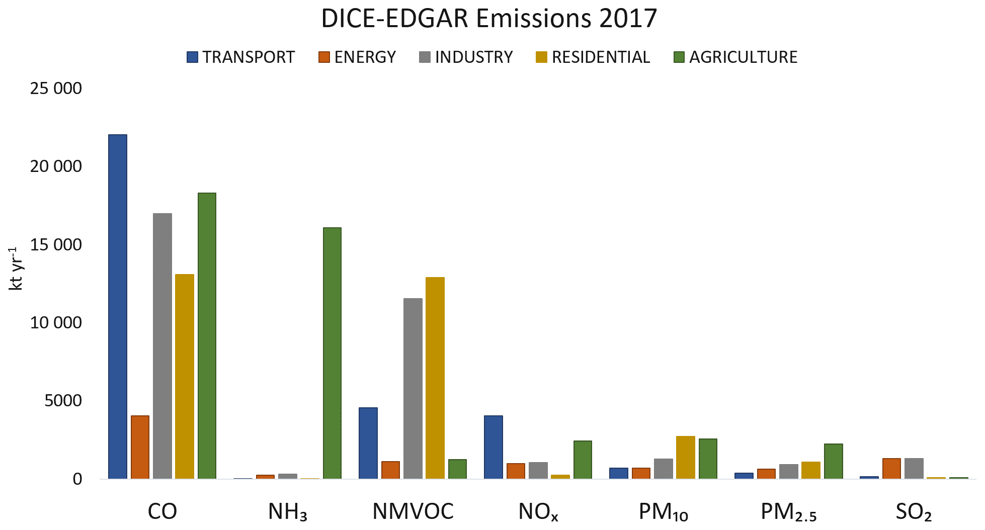
Figure 3 Annual totals for the DICE–EDGAR merged emission inventory for the year 2017 calculated using the 18 × 18 km spatial domain shown in Fig. 1.

Biogenic emissions and mineral dust considered in this work have been calculated in line by CHIMERE. The former are calculated using MEGAN model outputs, as described by Guenther et al. (2006), whereas the latter are calculated using the US Geological Survey (USGS) land use database provided by CHIMERE. The soil is represented by relative percentages of sand, silt, and clay for each model cell. The USGS database, called STATSGO-FAO, accounts for 19 different soil types recorded in the global database with a native resolution of 0.0083 × 0.0083^∘. To have homogeneous data sets, the STATSGO-FAO data are regridded to the CHIMERE simulation grids. For mineral dust emission calculations, the land use is typically employed to provide a desert mask specifying what surface is potentially erodible.

The emissions used in this work might not reflect the true values due to missing emission sources and the mismatch between the simulated time period and the date of the emission inventories. The lack of up-to-date national emission inventories collected at a sufficient resolution, in addition to the lack of research sources providing projections of emissions for 2017, meant that it was not possible to generate more detailed information about the anthropogenic sources of emissions for East Africa.

It is noted that the time stamps of the anthropogenic emissions and the validation period are different: the emissions are relative to the year 2013, whereas the observation used for the validation are for 2017. In the absence of additional data and due to the lack of national or local mitigation policies in the three countries, we assume that the differences between the time stamps do not make a large difference to the emission estimates. More detailed analysis of the emission sources and the implementation of possible mitigation policies at national and local levels could change this situation in the future.

Finally, we recall that one of the main objectives of the present work is to evaluate the performance of the WRF and CHIMERE models with respect to reproducing meteorology and air pollution levels in urban conurbations using the most up-to-date available data, thereby providing new insight into the state of the art of numerical modelling for air quality in this area of the world and highlighting possible improvements for future works.

2.4 Weather and chemistry observations

The WRF and CHIMERE models have been validated for a limited monthly period between 14 February and 14 March 2017. This period was chosen due to the availability of continuous measurements for the validation of both models. While WRF observations with a frequency from 3 to 6 h are available from the UK Met Office Integrated Data Archive System (MIDAS) database (MetOffice, 2012) for different locations, PM_2.5 observations that last over 1 month with a measurement frequency of 1 h from different environments (e.g. rural, urban, or roadside sites) are rarer.

The period chosen for the simulation of meteorology has to be representative of the average weather conditions of the analysed area and must avoid unusual weather conditions (e.g. extreme events) that could impact the physical and chemical processes described in the CTM as well as the final concentrations of secondary pollutants simulated. The February to March time period in East Africa does not have extreme temperatures (mean temperature of approximately 10–25 ^∘C depending on the country), and there is little rainfall that could affect the observations of weather conditions and PM_2.5 concentrations (FEWS NET, 2022). These conditions and the absence of alternative data covering a large time frame for the validation of CHIMERE constrained the period of simulation to the above-mentioned time span.

Observations of temperature, wind speed, and wind direction used for the validation of WRF were taken from the MIDAS database. Data from 11 weather stations, 3 respective stations for the Ethiopian (hereafter ETH2K; Fig. 2a) and Ugandan (hereafter UGA2K; Fig. 2b) domains and 5 for the domain of Kenya (hereafter KEN2K; Fig. 2c), were used to validate the simulations at a resolution of 2 × 2 km (Table 2).

Table 2 The UK Met Office ground weather stations used for the validation of the 2 × 2km domains. “Station no.” corresponds to the position of each station shown in Fig. 2a, b, and c including the PM_2.5 observation points in the urban domains of Addis Ababa, Kampala, and Nairobi used for the validation of CHIMERE model.

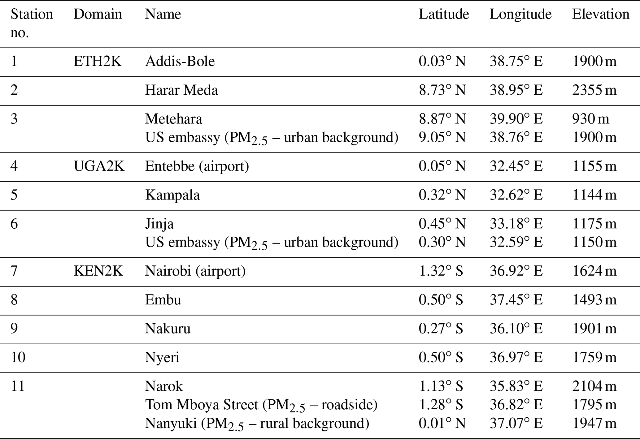
The ground stations are at different altitudes above sea level to a maximum of 2355 m (e.g. the Harar Meda station in Ethiopia – station no. 2 in Fig. 2a). The validation was performed by comparing model outputs with observations for the variables, namely surface temperature, wind speed and wind direction, and relative humidity. The latter, which is not originally available in the MIDAS data set, was calculated using the coefficients proposed by Alduchov and Eskridge (1996) based on hourly surface and dew point temperature observed values and then compared with modelled data obtained by WRF.

Hourly concentrations of PM_2.5 were used for the validation of CHIMERE for the three internal domains at 2 × 2 km (Fig. 2). For the city of Nairobi, data from roadside background site located at Tom Mboya Street were used (1.28^∘ S, 36.82^∘ E), while data from the rural background were provided by a site located in Nanyuki, Kenya (0.01^∘ N, 37.07^∘ E). Data from both field sites were obtained from the field sampling campaign performed by Pope et al. (2018). For the urban background locations of Addis Ababa and Kampala, hourly PM_2.5 concentrations were obtained from the air quality monitoring stations of the two US embassies in Ethiopia (9.05^∘ N, 38.76^∘ E) and Uganda (0.30^∘ N, 32.59^∘ E) using optical counters. Data from Uganda and Ethiopia were used to compare the configuration applied to CHIMERE for Kenya with the two other countries (Table 2).

2.5 Statistical parameters

In this work, we use different statistical operators to evaluate the performance of the WRF and CHIMERE models with respect to reproducing the main surface weather parameters and hourly and daily concentrations of PM_2.5 in different urban and rural environments. The statistical analysis for both WRF and CHIMERE has been done by calculating the statistics for each station individually and then averaging all station together. The calculation has been done on the original hourly values from observations and model outputs, and it considers hourly values from the model only if the corresponding hourly observation is present. The Pearson coefficient (R; Eq. 2), the index of agreement (IOA; Eq. 3), the mean fractional bias (MFB; Eq. 4), and the mean fractional error (MFE; Eq. 5) statistical parameters have been used for the calculations.

$$\begin{array}{}\text{(2)}& {\displaystyle }\begin{array}{rl}& R\\ & ={\displaystyle \frac{n\left({\sum }_{i=\mathrm{1}}^n{M}_i{O}_i\right)-\left({\sum }_{i=\mathrm{1}}^n{M}_i\right)\left({\sum }_{i=\mathrm{1}}^n{O}_i\right)}{\sqrt{\left[n{\sum }_{i=\mathrm{1}}^n{M}_i^{\mathrm{2}}-({\sum }_{i=\mathrm{1}}^n{M}_i{)}^{\mathrm{2}}\right]\left[n{\sum }_{i=\mathrm{1}}^n{O}_i^{\mathrm{2}}-({\sum }_{i=\mathrm{1}}^n{O}_i{)}^{\mathrm{2}}\right]}}}\end{array}\text{(3)}& {\displaystyle }\mathrm{IOA}=\mathrm{1}-\left[{\displaystyle \frac{{\sum }_{i=\mathrm{1}}^n{\left(O_i-M_i\right)}^{\mathrm{2}}}{{\sum }_{i=\mathrm{1}}^n{\left(\left|M_i-\stackrel{\mathrm{‾}}{O}\right|+\left|O_i-\stackrel{\mathrm{‾}}{O}\right|\right)}^{\mathrm{2}}}}\right]\text{(4)}& {\displaystyle }\mathrm{MFB}={\displaystyle \frac{\mathrm{1}}{n}}{\sum }_{i=\mathrm{1}}^n\left(M_i-O_i\right)/\left(\right(O_i+M_i)/\mathrm{2})\text{(5)}& {\displaystyle }\mathrm{MFE}={\displaystyle \frac{\mathrm{1}}{n}}{\sum }_{i=\mathrm{1}}^n\mathrm{|}{M}_i-O_i\mathrm{|}/\left(\right(O_i+M_i)/\mathrm{2})\end{array}$$

The MFB and MFE, in particular, are metrics specifically used for the evaluation of the numerical system for atmospheric chemistry and meteorology. They normalise the bias and the error for each model–observation pair by the average of the modelled and observed values before taking the final average. The advantages of these metrics are that the maximum bias and errors are bounded and that the impact of outlier data points are minimised. Moreover, the metrics are symmetric, thereby giving equal weight to concentrations that are simulated higher than observations and to concentrations that are simulated lower than observations.

The MFB and MFE have been expressed in terms of model performance “goals” and model performance “criteria” values, according to the methodology proposed by Boylan and Russell (2006). The performance goal for the modelling system is set as MFE ≤ 50 % and MFB ≤ ± 30 %. Within this range, the model performance with respect to reproducing the correct magnitude of the concentrations can be considered good. A second larger range of values (called criteria) is set as MFE ≤ 75 % and MFB ≤ ± 60 %. Values within this range correspond to average model performance. Finally, values within the range of MFE > 75 % and −60 % > MFB > +60 % represent poor representation by the model.

2.6 Model resolution and simulation design

The WRF and CHIMERE models run at spatial resolutions of 18 × 18, 6 × 6, and 2 × 2 km for meteorology and at 6 × 6 and 2 × 2 km for chemistry for the three East African domains. However, the statistical analysis shown in the following sections describes the validation results for the three internal domains at a resolution of 2 × 2 km, as these are the focus of the present work.

Ground weather stations from the MIDAS database, included in the 2 × 2 km domains of all countries, were analysed individually and are shown as the average of all stations. The time series and wind roses are relative to the closest stations from the MIDAS database to each urban city centre of the three capital cities, namely Addis-Bole (station no. 1 in Table 2), Kampala (station no. 5 in Table 2), and Nairobi airport (station no. 7 in Table 2).

Initially, the performance of CHIMERE was analysed for the domain of Kenya for which hourly concentrations of PM_2.5 were taken from two different sites (roadside and rural) from the field sampling campaign described by Pope et al. (2018). Secondly, the same configuration adopted for Kenya was used for Ethiopia and Uganda to test both the homogeneity of the emission rates under different urban conditions and the configuration chosen for CHIMERE under different urban and environmental conditions. At this stage of the validation, a daily threshold limit of 25 µg m⁻³ for PM_2.5, provided by WHO (WHO, 2005), was used to quantify the number of exceedances observed and modelled by CHIMERE for the three cities.

The validation process was hindered by the highly variable quantity and quality of available meteorological data. The majority of the weather observations are provided on a 3-hourly basis, with varying amounts of missing data. Despite this, the statistical evaluation of WRF was performed by comparing model simulations and observations only when the latter were available. We recall that the objective of this work aims to test the performance of a modelling system with respect to the simulation of air quality at high resolution for East Africa, updating and/or using the available input data available and assessing the possible adoption of these tools for air quality policymaking with this extent of data.

3 Results and discussion

3.1 Validation of the WRF simulations

In order to assess the performance of WRF in simulating surface temperature, relative humidity, wind speed, and wind direction, the model simulation outputs were compared with all of the available ground weather station data available for the period of analysis (14 February to 14 March 2017).

3.1.1 Statistical evaluation of WRF performance

A statistical analysis, in terms of the mean fractional bias (MFB), mean fractional error (MFE), index of agreement (IOA), and Pearson coefficient (R), was carried out to compare modelled and observed values for the domain at a 2 × 2 km resolution by averaging the observed and modelled values from all of the stations present in each domain (Table 3). We recall that the number and location of the stations is variable between the three domains (three respective stations for ETH2K and UGA2K and five stations for KEN2K).

The results of the statistical analysis show that WRF more successfully reproduces the mean levels of surface temperature for the Ethiopian (ETH2K) and Ugandan (UGA2K) domains, with a mean underestimation over the three domains of 1.4 and 1.5 ^∘C respectively, then for Kenya (KEN2K), where it shows an underestimation of 4.1 ^∘C. However, the higher bias in surface temperature found in the average of all five Kenyan stations is highly driven by particularly poor representation of this variable at the observation point of Narok (station no. 11 in Fig. 2c), where the bias between the simulated and observed values is 10.9 ^∘C. A reason for this bias may be the fact that the location of the above-mentioned station is at the highest altitude of all of the Kenyan weather stations (2104 m a.g.l.). Narok is located around 140 km west of Nairobi, and the high bias in temperature should not have any effect on the levels of temperature modelled in the capital of Kenya, where the bias for the individual station of Nairobi (station no. 7 in Fig. 2c) found was 1.3 ^∘C.

WRF overestimates relative humidity by 0.2 % in KEN2K, whereas it underestimates relative humidity by 6.4 % in ETH2K and by 7.5 % in UGA2K (Table 3). Wind direction for the three domains show the presence of northerly winds in UGA2K, which is correctly captured by the model, with a difference of around 4^∘ in comparison with the observations; an average easterly wind component in KEN2K, which is partially reproduced by the model, that allocates the average wind direction to a more south-easterly component, with a difference of around 40.2^∘; and a closer modelled and observed average wind direction in ETH2K, with a difference of 4.2^∘ and a south-easterly prevailing wind component. The observed and modelled wind speeds in UGA2K, KEN2K, and ETH2K suggest a model overestimation of 0.9, 0.8, and 0.2 m s⁻¹ respectively (Table 3).

Table 3 Statistical analysis of relative humidity, surface temperature, wind speed, and wind direction averaged over all of the available weather stations for the second nested domains of UGA2K, KEN2K, and ETH2K at a 2 × 2 km resolution. The mean observed and modelled values, the Pearson coefficient (R), the index of agreement (IOA), the mean fractional bias (MFB), and the mean fractional error (MFE) are shown.

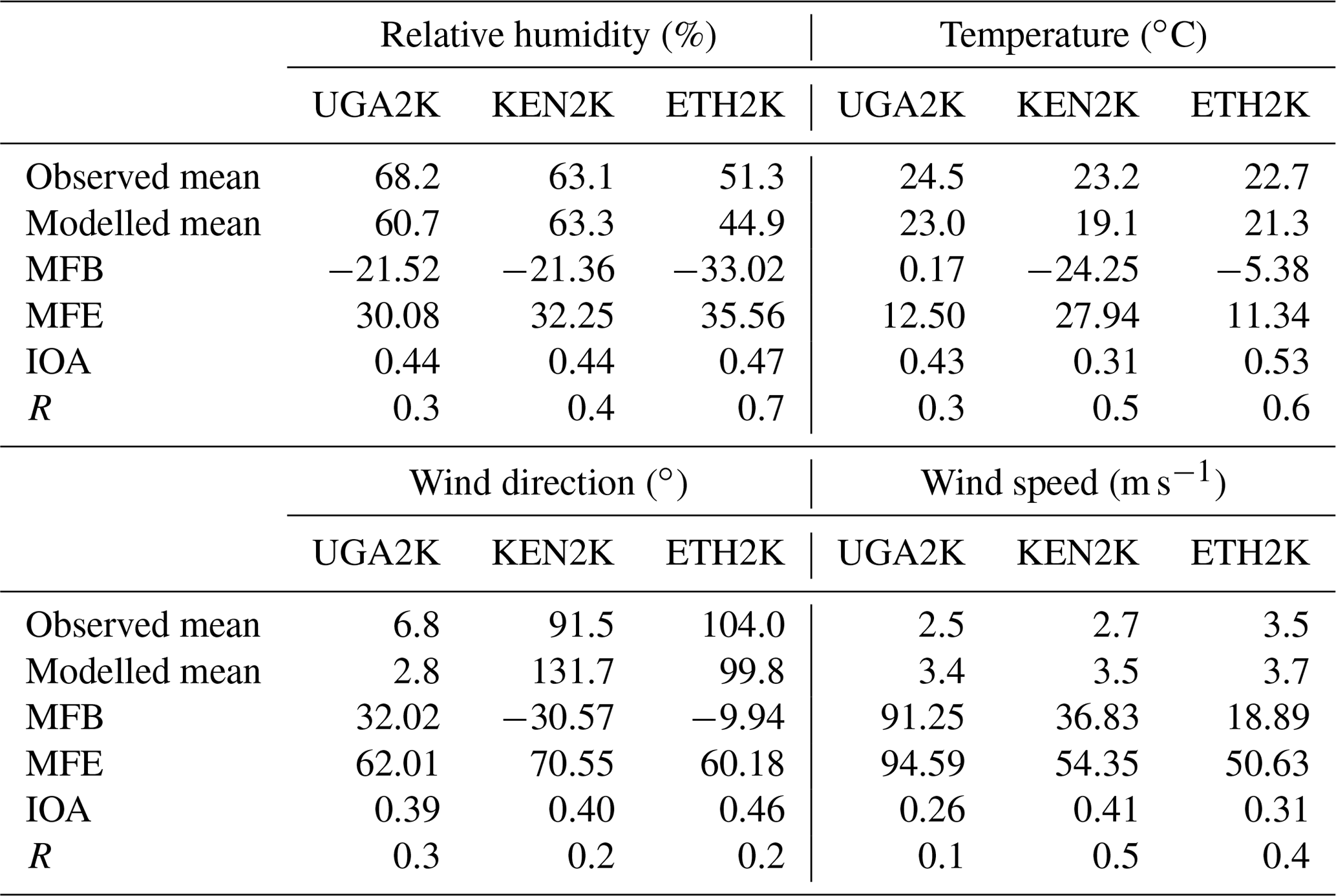
The mean fractional error calculated for the three domains is within the limit of the goal range for both surface temperature and relative humidity, with values between 30 and 35 for the former and 11 and 27 for the latter variable. On the other hand, the MFE values for wind speed and direction are more variable depending on the domain. While MFE values for wind direction were within the criteria range for all domains, only KEN2K and ETH2K were within this range for wind speed; the wind speed in UGA2K was found to be outside of the acceptability range with respect to model performance (Table 3).

The same analysis done taking the mean fractional bias in account shows values within the goal range for surface temperature for the three domains, although overestimated by the model for UGA2K (0.17) and underestimated for ETH2K (−5.38) and KEN2K (−24.25). The same behaviour was also found for the relative humidity: it is underestimated in the three domains but has MFB values within the goal criteria. Finally, wind speed and direction are both found to be within the MFB goal range for ETH2K, KEN2K shows values of both variables within the criteria range, and UGA2K shows wind direction values in the criteria range but wind speed values outside of the acceptability range with respect to model performance (Table 3).

The calculated Pearson coefficient (R) shows the capability of the model with respect to reproducing the minimum and maximum peaks of different variable values. The R values were found to vary between 0.1 and 0.7 for the three domains. The reproduction of the maximum and minimum relative humidity values was better for ETH2K, where the R value was found to be approximately 0.7, whereas the lowest R values were found for UGA2K (0.3). A similar trend was also found in the description of the surface temperature, with better reproduction of the maximum and minimum values in ETH2K (0.6), followed by KEN2K (0.5) and UGA2K (0.3). For wind speed, the highest R coefficient value was found for KEN2K (0.5), and the lowest value was found for for UGA2K (0.1). For wind direction, the highest R value was found for UGA2K (0.3), while values of approximately 0.2 were found for the other two domains (Table 3).

Finally, the evaluation of the index of agreement (IOA) shows values for surface temperature of between 0.31 (KEN2K) and 0.53 (ETH2K) and values for relative humidity of between 0.44 and 0.47 for the three domains. For wind speed and direction, the IOA varies between 0.39 (UGA2K) and 0.46 (ETH2K) for the former and between 0.26 (UGA2K) and 0.41 (KEN2K) for the latter. The comparison of the index of agreement between the three domains suggests that model performance is better with respect to reproducing drier areas such as ETH2K and KEN2K in comparison with UGA2K where the influence of the Lake Victoria seems to impact the overall statistical analysis. The performance of WRF with respect to reproducing the general conditions of wind speed and direction between the three domains is more variable.

3.1.2 Hourly variation in temperature and relative humidity

The three Met Office stations providing weather observations closest to the urban areas of Addis Ababa, Kampala, and Nairobi have been analysed individually in the form of hourly time series of surface temperature and relative humidity as well as wind roses for wind speed and direction.

The hourly surface temperature and relative humidity are shown in Fig. 4 for the three ground weather stations closest to the centre of the three cities: Addis-Bole (station no. 1 in Fig. 2a), Kampala (station no. 5 in Fig. 2b), and Nairobi (station no. 7 in Fig. 2c).

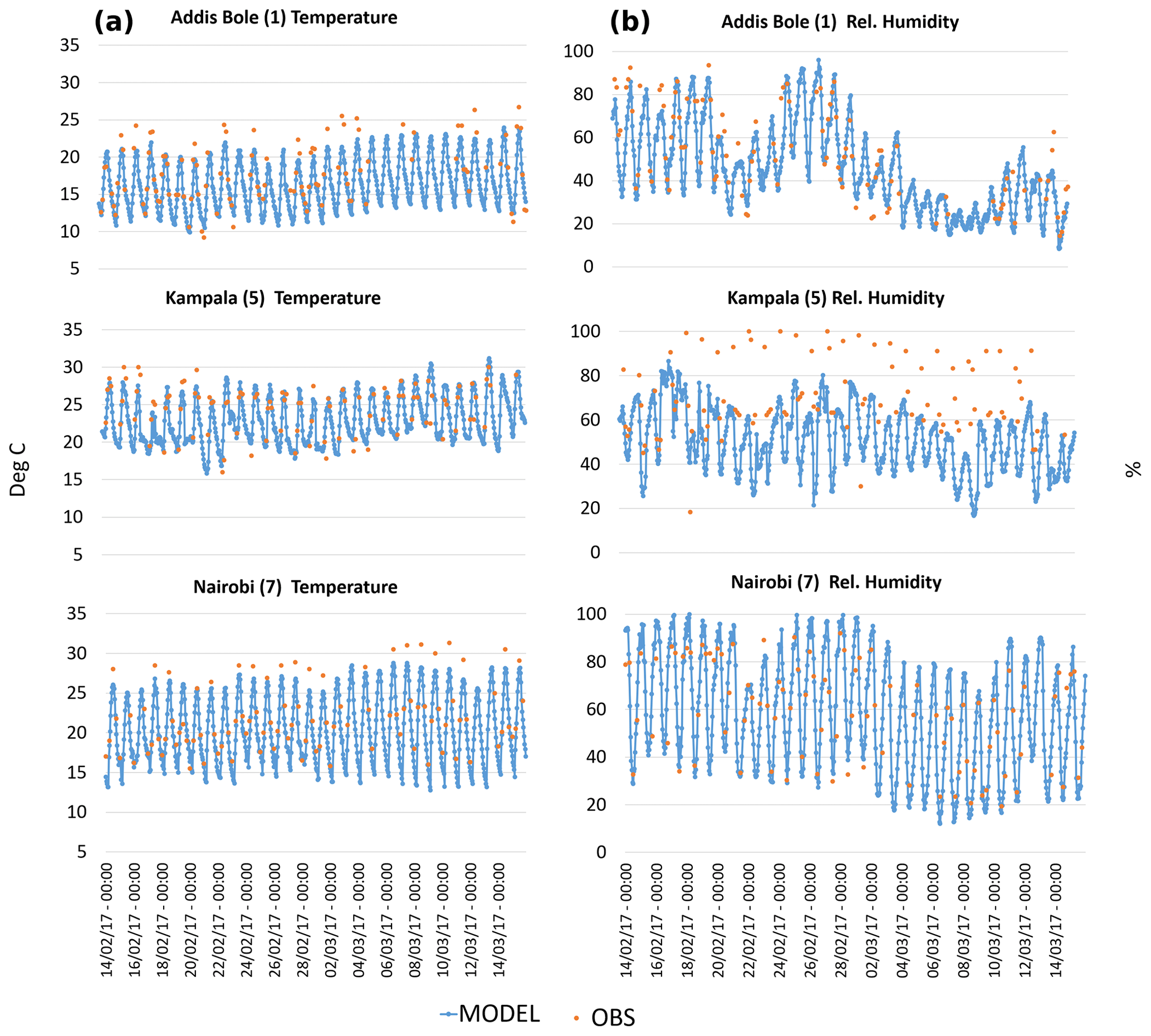
Figure 4 Hourly time series of (a) surface temperature and (b) relative humidity for the closest ground weather stations to the urban centres of Addis Ababa (station no. 1 in Fig. 2a), Kampala (station no. 5 in Fig. 2b), and Nairobi (station no. 7 in Fig. 2c). Comparisons between the modelled values (blue lines) obtained from the 2 × 2 km domains and hourly observations (orange spots) from the MIDAS database are shown.

The temperature range observed at the three stations was between 9 and 27^∘ C for Addis-Bole, between 16 and 31^∘ C for Kampala, and between 16 and 33^∘ C for Nairobi. By inspection of Fig. 4, it can be seen that the WRF model is able to reproduce the main diurnal cycle of variation in temperature and relative humidity for the three ground weather stations. Surface temperature peaks are slightly underestimated by the model for the three stations, with a small mean bias at the three stations of between −0.06 and −0.1^∘ C. The highest agreement between the modelled and observed values is for Kampala, whereas the model tends to almost systematically underestimate the diurnal peaks of surface temperature for the Addis-Bole and Nairobi stations.

The mean relative humidity observed at the three stations shows different ranges of excursion from the model predictions depending on the characteristics of the environment: Addis-Bole station shows higher variation, from 15 % to 98 %; values at Nairobi station vary between 17 % and 98 %; and values at Kampala vary between 19 % and 99 %. From Fig. 4, it may be seen that relative humidity variation over time is correctly captured by WRF for the Nairobi and Addis-Bole stations; however, both the diurnal peaks and the night-time minimum values seem not to be correctly reproduced by the model, which tends to overestimate the former and underestimate the latter with a bias of between −0.1 % and 0.004 %. Moreover, WRF appears systematically to underestimate the relative humidity for the Kampala station, showing a mean negative bias. Different reasons could affect the underestimation of the relative humidity at this station. The sensitivity of the WRF model to the land use data (Teklay et al., 2019) connected with the proximity of Kampala to Lake Victoria, which is a massive inland body of water (surface area of 68 800 km²), could influence the local variation in relative humidity in ways which are not well reproduced by the model. The influence of Lake Victoria and of the Kampala's complex topography on measurements of relative humidity has previously been highlighted by Singh et al. (2020) in relation to monthly visibility connected with PM levels. It has to be noted that relative humidity was calculated from surface temperature and dew point values, following Alduchov (1996), and not directly sampled. A better agreement in the simulation of relative humidity from WRF can be found for the station of Entebbe (station no. 4 in Fig. 2b), where the mean normalised bias shows a small underestimation of 0.04 %.

Wind speed and direction from the urban stations of Addis Bole (station no. 1 in Fig. 2a), Kampala (station no. 5 in Fig. 2b), and Nairobi (station no. 7 in Fig. 2c) are shown in Fig. 5 in the form of wind roses. For Nairobi, WRF can reproduce average wind directions in close agreement with the observed data for the analysed period, showing the predominant presence of north-north-easterly winds with high speed (> 4.0 m s⁻¹). Wind speed observations from the ground weather station of Kampala also suggest a strong southerly wind component (> 4.0 m s⁻¹), while the model seems to reproduce a similar magnitude with respect to wind speed but with a larger range of directions, from the south-south-east to the south-south-west. For Addis Ababa, WRF seems able to capture and reproduce the main wind directions observed for the simulated period (e.g. easterly and north-easterly winds). However, slower winds (between 0.2 and 2.0 m s⁻¹) with a strong north-northeasterly component do not seem to be replicated by the model for the station located inside the capital of Ethiopia.

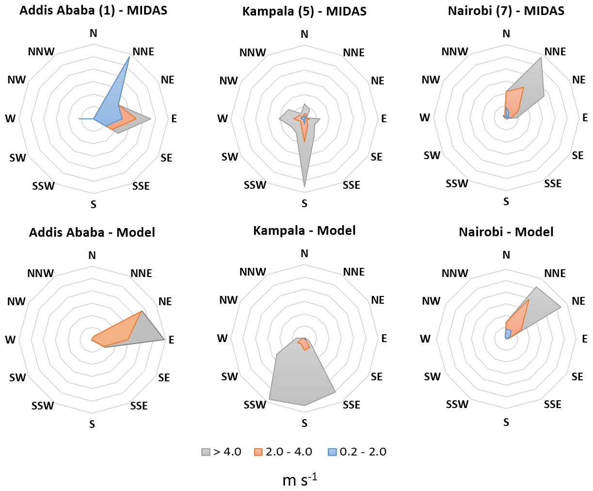
Figure 5 Averaged wind roses for the whole analysis period (14 February to 14 March 2017) from the closest ground weather stations to the urban centres of Nairobi (station no. 7 in Fig. 2c), Kampala (station no. 5 in Fig. 2b), and Addis Ababa (station no. 1 in Fig. 2a) (MIDAS observations, top row) and from WRF simulations (model outputs, bottom row).

The lower agreement in the reproduction of the wind speed and direction for the Addis-Bole and Kampala stations can be connected to the particular locations of both stations. The difference in the location of the observations can, in fact, influence rapid changes in the direction and speed that are recorded locally but are not reproduced by the model. In the case of Kampala, the Entebbe airport is located near the coast of Lake Victoria where the local wind conditions are more susceptible to variation and can be erroneously reproduced by the model. In the case of Addis-Bole, the only station in an urban area, the urban topography and possible canyon effects of the wind can be not well captured by the model; instead, the model reproduces a more constant range of wind speed and direction and does not account for quick variations at low speed that are observed at the station.

The results obtained from the validation of the meteorological simulations performed over East African domains using WRF show that the model is, on average, able to reproduce all four of the considered variables, providing values close to the observed data in the 2 × 2 km domains, with variable agreement between the three cities. The highest agreement in the weather analysis has been found for surface temperature, with similar biases to Kerandi et al. (2017), and relative humidity, similar to Pohl et al. (2011), which is sufficiently accurate to be able to use these values for the physical calculations done by the chemistry transport model.

Nevertheless, more detailed analysis of the urban weather stations revealed discrepancies in the reproduction of relative humidity and wind direction for Kampala station (UGA2K) that could affect the deposition, removal, and transport processes simulated by CHIMERE; this will be the subject of future investigation in order to further improve the meteorological performance of WRF. Even if the bias found for some variables in the calculation of the averaged statistics over all stations was high, the individual weather stations close to the urban areas of interest showed smaller bias values as well as MFB and MFE values within the goal or criteria range of performance; therefore, these values are considered acceptable for the simulations.

3.2 Validation of the CHIMERE simulations

The CHIMERE validation focused on the hourly levels of PM_2.5 modelled at the two observation sites in the KEN2K domain, which are representative of a respective roadside site and a rural background site, and also at the urban background observational sites of the US embassies of Kampala (UGA2K) and Addis Ababa (ETH2K). The performance of CHIMERE was also analysed in terms of the mean fractional error (MFE), the mean fractional bias (MFB), and the Pearson coefficient (R) against the different average PM_2.5 concentration levels at the four observation points in order to evaluate the response of the model with respect to reproducing low and high hourly concentration levels in comparison to observed values.

The validation of CHIMERE was done for the domains at the highest resolution (2 × 2 km), despite the availability of emissions at a similar spatial resolution. This choice was motivated by the necessity to validate the reliability of the model against observed data from particular locations with different backgrounds. In order to better configure the model to represent the different urban and rural environments, it is necessary to consider the uncertainties in the model representation with respect to an observation point. One cause of uncertainty when comparing modelling outputs with observations is the difference between a point measurement and a volumetric grid-cell-averaged simulated concentration (Seinfeld and Pandis, 2016). On the one hand, the extent of a measurement point, in fact, represents only the extent of the nearby points or an average concentration in a specified area. On the other hand, a surface-level modelling grid typically has the highest resolution of 1 km with a vertical height of between 20 and 40 m, and the concentration represented by the model is the average over the entire grid cell.

In the particular case of the East African domains, CHIMERE simulates concentration values representative of an average of 36 km² at a coarse resolution (e.g. 6 × 6 km), which is difficult to compare with observations taken at a particular point. If the spatial resolution is increased to 2 × 2 km, the average value inside each grid cell will be representative of a smaller area (e.g. as 4 km²) whose average value can be closer compared to an individual observation point.

3.2.1 Statistical evaluation of model performance

The absolute bias between mean observed and modelled concentrations of PM_2.5 shows a model overestimation by between 0.01 and 3.7 µg m⁻³ for the KEN2K domain for Nanyuki and Nairobi respectively as well as for Addis Ababa (0.6 µg m⁻³). On the contrary, the model underestimates PM_2.5 by 7.2 µg m⁻³ for the UGA2K domain (Kampala) (Table 4).

The MFB and MFE for the two Kenyan observation points, Nairobi (roadside site) and Nanyuki (rural site), were found to be within the goal performance criteria in both cases, with MFE values of ≤ 50 % and MFB values of ≤ ± 30 %. The respective hourly MFB and MFE values were 4.88 and 25.39 for Nairobi and 3.36 and 8.33 for Nanyuki, while the respective values found for the daily analysis were 0.1 and 1.99 for Nairobi and 1.08 and 4.73 for Nanyuki.

The MFB and MFE analysis for the urban background site in Addis Ababa showed values within the range of the goal criteria for both the hourly (2.93 and 29.99 for MFB and MFE respectively) and daily analysis (8.23 and 2.86 respectively). Finally, for the urban background site of Kampala, the MFB was found to be within the goal criteria for both the daily (−11.28) and hourly (−7.60) analysis; for the MFE, the hourly analysis showed a value within the criteria range (32.99), but the daily MFE value was within the goal performance range (22.06) (Table 4).

Table 4 Hourly and daily statistical evaluation of CHIMERE model performance for the cities of Nairobi against ASAP observed data and against US embassy data for the cities of Addis Ababa and Kampala.

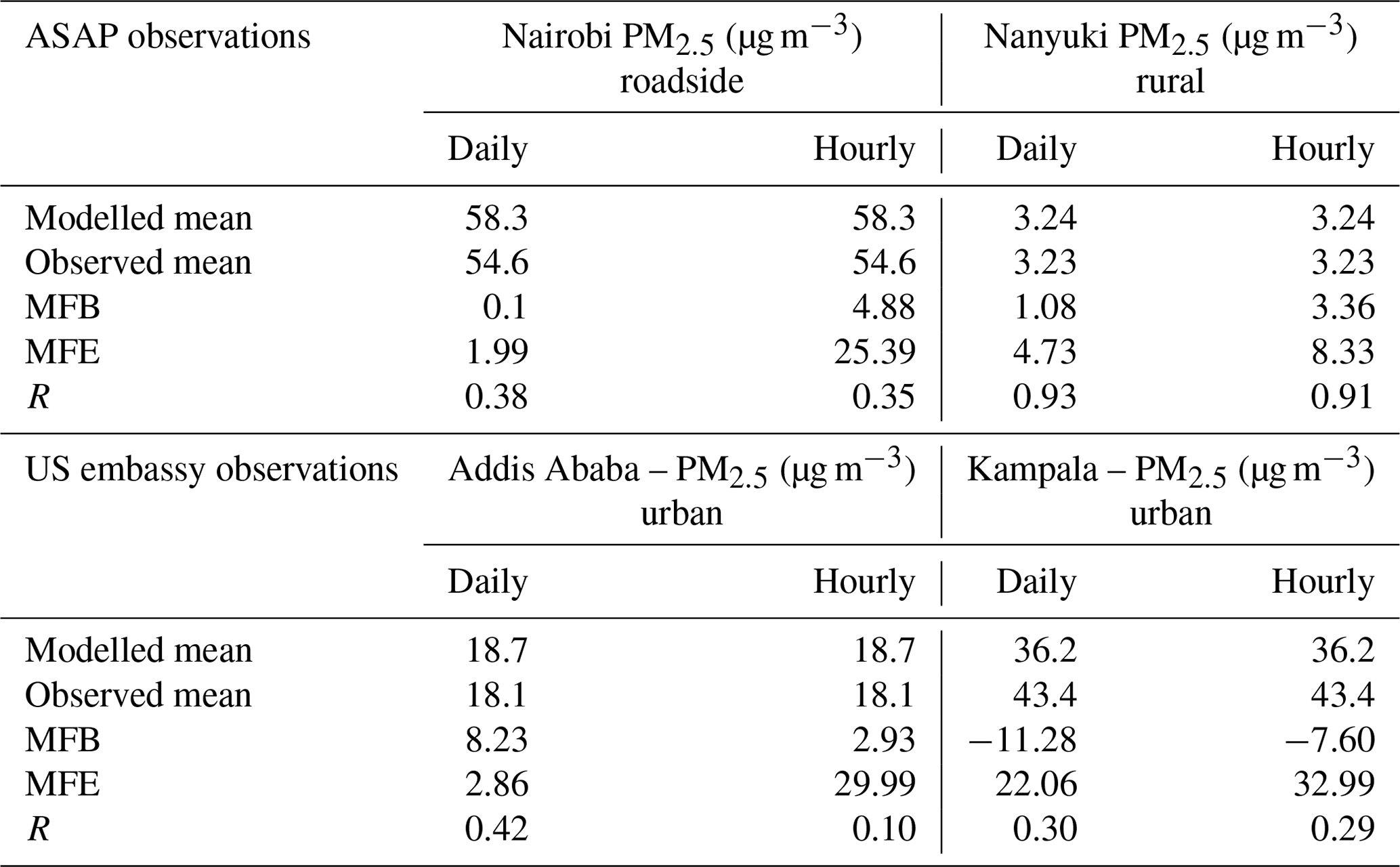
The highest Pearson coefficient (R) values were found in Nanyuki, with hourly and daily values of between 0.91 and 0.93. The roadside site of Tom Mboya Street in Nairobi had R values of between 0.35 and 0.38, while the urban background sites of Addis Ababa and Kampala had lower agreement at an hourly level (R values were between 0.10 and 0.29 respectively) than at a daily level (R values of between 0.42 and 0.30 respectively).

In general, the statistical analysis demonstrates that the model can reproduce the daily pattern of the hourly changes in concentrations for the two pollutants at the three urban/roadside sites and the rural site considered. The low R coefficient values obtained for the urban domains at the hourly level suggest that sources of anthropogenic emissions affecting urban air quality are still missing from the current emission inventory. Further work will be focused on the improvement of the magnitude of the emissions in order to better match the observed levels of particulate matter concentrations at the urban level. Nevertheless, considering the daily average concentrations at the urban sites, the R coefficients were found to be between 30 % and 42 %, suggesting that CHIMERE better reproduces the concentrations of PM_2.5 using daily values compared with hourly values.

The performance of CHIMERE varies between the Kenyan, Ugandan, and Ethiopian domains. The performance of the model has been optimised during the validation for the simulation of hourly concentrations of PM_2.5 in Kenya, and the same configuration has been applied to the Ugandan and Ethiopian domains in order to compare the reliability of the model. The difference in performance can be connected to different reasons: (1) the difference in the sampling methods used for the two sites in Kenya compared with the measurements taken at the US embassies in Kampala and Addis Ababa, and (2) the location of the observation sites in the cases of the US embassies and/or the possible influence of local sources not accounted for in the emission inventories.

The agreement between the simulated and observed values is highest at the Nanyuki site. This location was chosen by Pope et al. (2018) as rural site in an area with minimum local air pollution, which is useful to calculate the net urban increment by subtracting the rural background concentrations of Nanyuki from the urban concentrations in Nairobi. Therefore, they intentionally chose a site that would experience very low average concentrations. The model is able to reproduce this low level of contamination well (close to reality), and it is also able to reproduce contamination peaks on particular days in February that were probably generated elsewhere (see Sect. 3.2.2).

The MFB and MFE analyses have also been conducted at an hourly level, comparing modelling outputs and observations from all six sites in relation to the magnitude of hourly concentrations (Fig. 6).

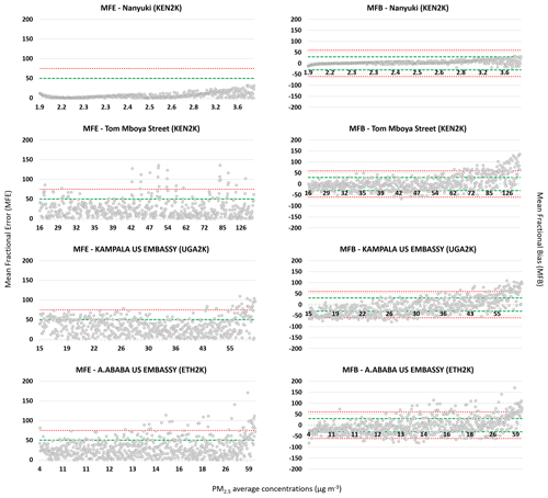
Figure 6 The hourly mean fractional bias (MFB) and mean fractional error (MFE) values calculated for the Tom Mboya Street and Nanyuki (KEN2K), Kampala US embassy (UGA2K), and Addis Ababa US embassy (ETH2K) locations for the analysis period against hourly concentrations of PM_2.5. The green lines represent the MFB range ±30 % and the MFE limit of 50 %, for which the model performance can be considered reliable; the red lines represent the MFB range ±60 % and the MFE limit of 75 %, for which model performance can be increased by diagnostic analysis of the chemical precursors of PM_2.5.

There are some MFB values outside of the criteria range for PM_2.5 for the urban sites of Addis Ababa and Kampala and for the roadside site of Tom Mboya Street in Nairobi. In terms of the upper limit (MFB > 60 %), these values tend to be concentrated between 60 and 130 µg m⁻³ for Tom Mboya Street, between 40 and 55 µg m⁻³ for Kampala, and between 13 and 59 µg m⁻³ for Addis Ababa (Fig. 6). A much smaller number of MFB values for the Addis Ababa and Kampala sites are less than the lower criteria limit, and these values tend to be for lower concentrations of between 10 and 26 µg m⁻³.

MFE values outside of the ranges of criteria are between 42–55 and 80–130 µg m⁻³ for Tom Mboya Street, between 43 and 60 µg m⁻³ for Kampala, and between 13 and 59 µg m⁻³ for Addis Ababa (Fig. 6). The latter two sites present more variability in the MFB and MFE compared with the two Kenyan sites where a common positive bias of the model in reproducing the highest concentration levels is visible. Therefore, the reliability of the model is higher for the Kenyan domain, for both the rural and roadside site, than for the two urban background sites in Uganda and Ethiopia.

The overall performance of the model against different concentration levels is summarised in Table 5. The PM_2.5 reproduced at the two sites in KEN2K shows a higher percentage of values within the MFB and MFE performance goals for the rural site of Nanyuki than for Tom Mboya Street (e.g. 97 % compared with 69 % and 99 % compared with 88 % for the MFB and MFE measures respectively). For the criteria measure, the corresponding percentages for the respective MFB and MFE measures are 2 % vs. 22 % and 1 % vs. 7 % (Table 5).

The percentages for the urban sites of Kampala and Addis Ababa show a lower agreement between the model and observations. For Kampala, according to the MFB measure, 48 % of the values are within the goal range, 37 % of the values are within the criteria range, and 15 % of the values are outside of the acceptability range. For Addis Ababa, according to the MFB criteria, 57 % of the values are within the goal range, 30 % of the values are within the criteria range, and 13 % of the values are outside of the acceptability range. In terms of the MFE measure, 74 % and 80 % of values for the two respective above-mentioned cities are within the goal range, 16 % and 11 % within the criteria range, and 10 % and 9 % outside of the acceptability range (Table 5).

Table 5 The hourly mean fractional bias (MFB) and mean fractional error (MFE) percentage of points within the goal range (Goal), within the diagnostic range (Criteria), and outside of the reliability criteria range (Out) from model outputs extracted from the four analysed locations.

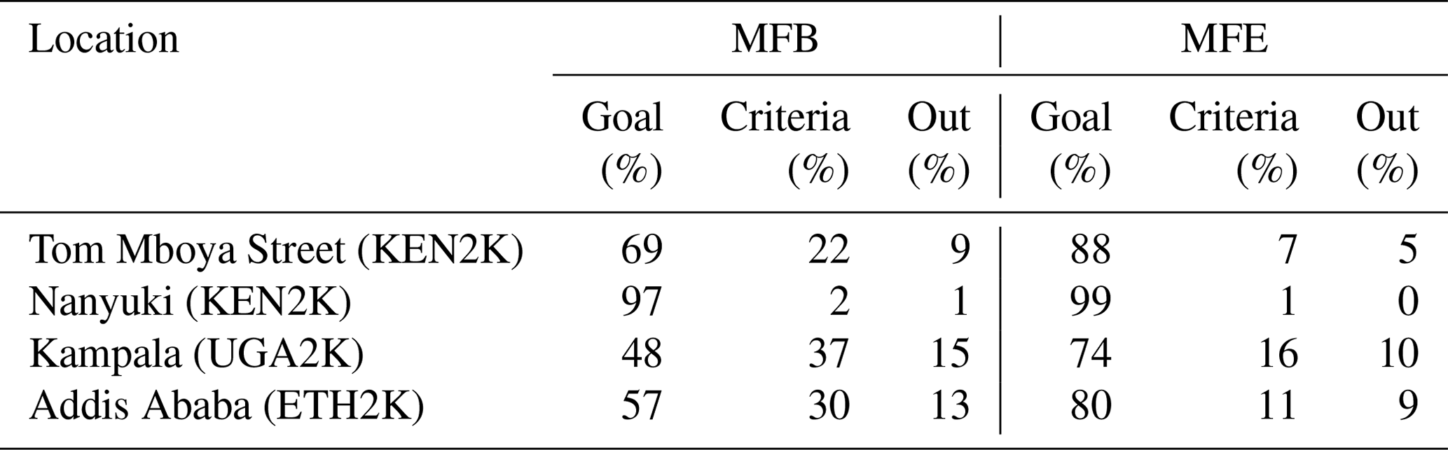
According to the methodology proposed by Boylan and Russel (2006), the performance of a modelling system is fairly good for PM_2.5 representation if about 50 % of the points are within the goal range and a large majority are within the criteria range. From the analysis of the four sampling sites, the MFB values within the goal range are 69 % for Tom Mboya Street, 97 % for Nanyuki, 57 % for Addis Ababa, and only 48 % for Kampala. Similarly, for the MFE measure, the percentage of values within the goal range are 99 % for Nanyuki, 88 % for Tom Mboya Street, 80 % for Addis Ababa, and 74 % for Kampala. This demonstrates that the performance of the model can be considered to be satisfactory (Table 5).

Finally, the reason for the presence of values outside of the criteria range at both high and low PM_2.5 concentrations in the Addis Ababa and Kampala simulations can be connected to the representation of the original PM emissions in the combined inventory. It is possible that CHIMERE is not able to correctly reproduce all of the chemical processes involved in the secondary formation of the inorganic and organic individual components of PM_2.5 with the extent of the present input data. Moreover, the possible misrepresentation of local emission sources not reproduced in DICE–EDGAR can also affect the performance of the model. Finally, the different locations of the urban background observation sites and the sampling techniques for PM observation can also play a key role in the correct detection of the concentrations.

3.2.2 Hourly variation in PM_2.5 at urban and rural sites in Kenya

The hourly modelled variation in the PM_2.5 levels obtained by CHIMERE compared with observations is shown for the urban sampling site of Tom Mboya Street in Nairobi and for the rural site of Nanyuki (Fig. 2c).

By inspection of Fig. 7 it can be seen that CHIMERE is generally able to reproduce the daily variation in PM_2.5 across the simulated period at both sites. The magnitude of the emissions adopted seems to be suitable for both the roadside area of Tom Mboya Street and the rural background site of Nanyuki, with higher agreement shown by the latter. CHIMERE captures only part of the daily peak observed at Tom Mboya Street, with a comparable magnitude but the misrepresentation of some peaks. In particular, it models higher hourly peaks than those observed, as previously mentioned in the MFB and MFE analysis.

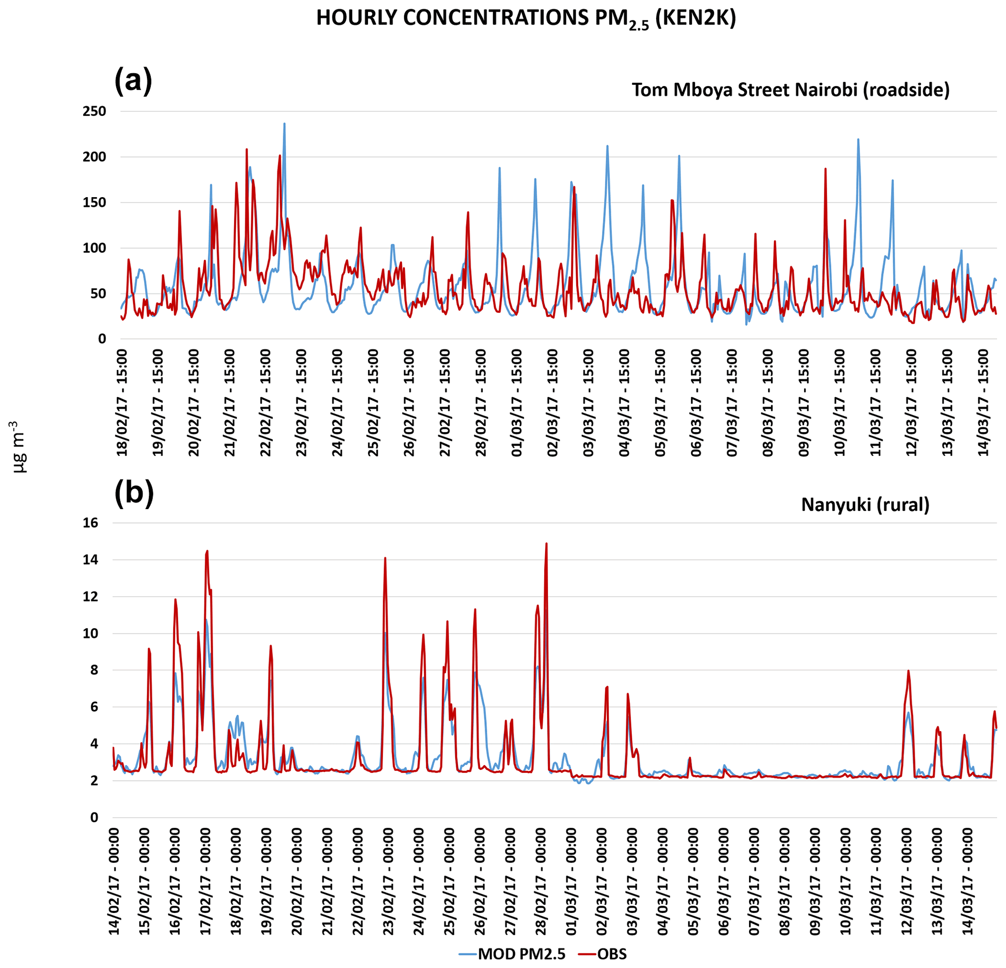
Figure 7 The hourly time series for PM_2.5 from (a) the roadside of Tom Mboya Street and (b) the rural site of Nanyuki based on CHIMERE model output (blue line) and observed values from Pope et al. (2018) (red line) for the analysed period The simulation started on 14 February. For the Tom Mboya Street site, only the period of time between 18 February and 14 March (period for which observations are available) is shown in the time series.

The misrepresentation of some high peaks at Tom Mboya Street is possibly due to a number of different reasons. Firstly, is important to recall that the point measurements and relative observed concentrations are representative of a smaller portion of space compared with the grid cell concentrations modelled. In this particular case, the comparison is between a roadside site subjected to possible additional local sources of PM_2.5 that are not accounted for in the emissions and, thus, not correctly reproduced by CHIMERE. On the other hand, a few of the modelled peaks were overestimated. This can be addressed by an improved temporal description of the emissions and their magnitude in comparison to reality. As mentioned previously, the anthropogenic emissions used in this work were the most up-to-date available at the time, but there is inevitably some difference between the measured data due to the temporal difference between the inventories and the measurements. Nevertheless, there is reasonable agreement between model outputs and observed concentrations for the majority of the analysed period, highlighting the reliability of CHIMERE with respect to describing the hourly concentration trends for a roadside site with expected high levels of PM_2.5 contamination.

Similarly, at the rural site of Nanyuki, the model seems to correctly reproduce the hourly variation in the concentrations during the whole period, only underestimating the maximum peaks at the beginning of February and during the last 4 days of simulation in March. (Fig. 7). The site shows a different magnitude with respect to the concentrations of PM_2.5 when comparing the February and March periods. While hourly concentrations are around 3–4 µg m⁻³ between 4 and the 10 March, the concentrations of PM_2.5 are more than 2 times higher prior to and following to this period of time. This behaviour is visible in both the observations from the site (red line in Fig. 7b) and the model outputs obtained using CHIMERE (blue line in Fig. 7b).

Nanyuki was chosen by Pope et al. (2018) as rural site in a location with minimum influence from local air pollution. Data from Nanyuki were used for the calculation of the net urban increment via the subtraction of the rural background concentration from Nanyuki from the urban concentrations in Nairobi. The average concentrations of around 3–4 µg m⁻³ in the period between 4 and 10 March are rural background levels in the absence of any external influence from meteorological parameters and in the absence of local sources. However, the presence of higher hourly peaks before and after the 4 to 10 March period can be linked to different reasons: the presence of local emission sources contributing to the peaks or the dispersion of polluted air masses from elsewhere towards the site of Nanyuki.

It is important to note that the model and observations seem to agree particularly well regarding the description of the difference in magnitude between the different time periods at the above-mentioned site, excluding the possibility that the observed values can be influenced by local emission sources not accounted for in the emission inventory. It seems more likely, however, that those concentration levels are transported to Nanyuki from neighbouring areas with higher levels of PM_2.5 contamination. To investigate this possible role of PM_2.5 dispersion towards Nanyuki, we consider the closest MIDAS weather station to the sampling area of Nanyuki, which is located in the town of Nyeri (0.43^∘ S, 36.95^∘ E; altitude 1916 m a.g.l.; station no. 10 in Fig. 2). Nyeri is only 60 km from the Nanyuki site and is situated between Mount Kenya (0.10^∘ S, 37.30^∘ E; altitude 4341 m a.g.l.) to the west and the Aberdare Range (0.46^∘ S, 36.69^∘ E; altitude 3441 m a.g.l.).

The daily average concentrations observed at the Nanyuki sampling site have been compared with the daily mean wind speed and wind direction values observed at the Nyeri MIDAS station and with the daily mean values of wind speed and wind direction modelled by WRF in Nanyuki (Fig. 8). The period between 4 and the 10 March, when the daily average concentrations of PM_2.5 observed in Nanyuki were around 2.2 µg m⁻³, corresponds to higher-wind-speed conditions (between 4 and 5 m s⁻¹) mainly coming from the north-east (around 60^∘). During the same period, the modelled wind speed at Nyeri was low (between 1 and 2.5 m s⁻¹) and mainly consisted of a westerly component (between 220 and 300^∘).

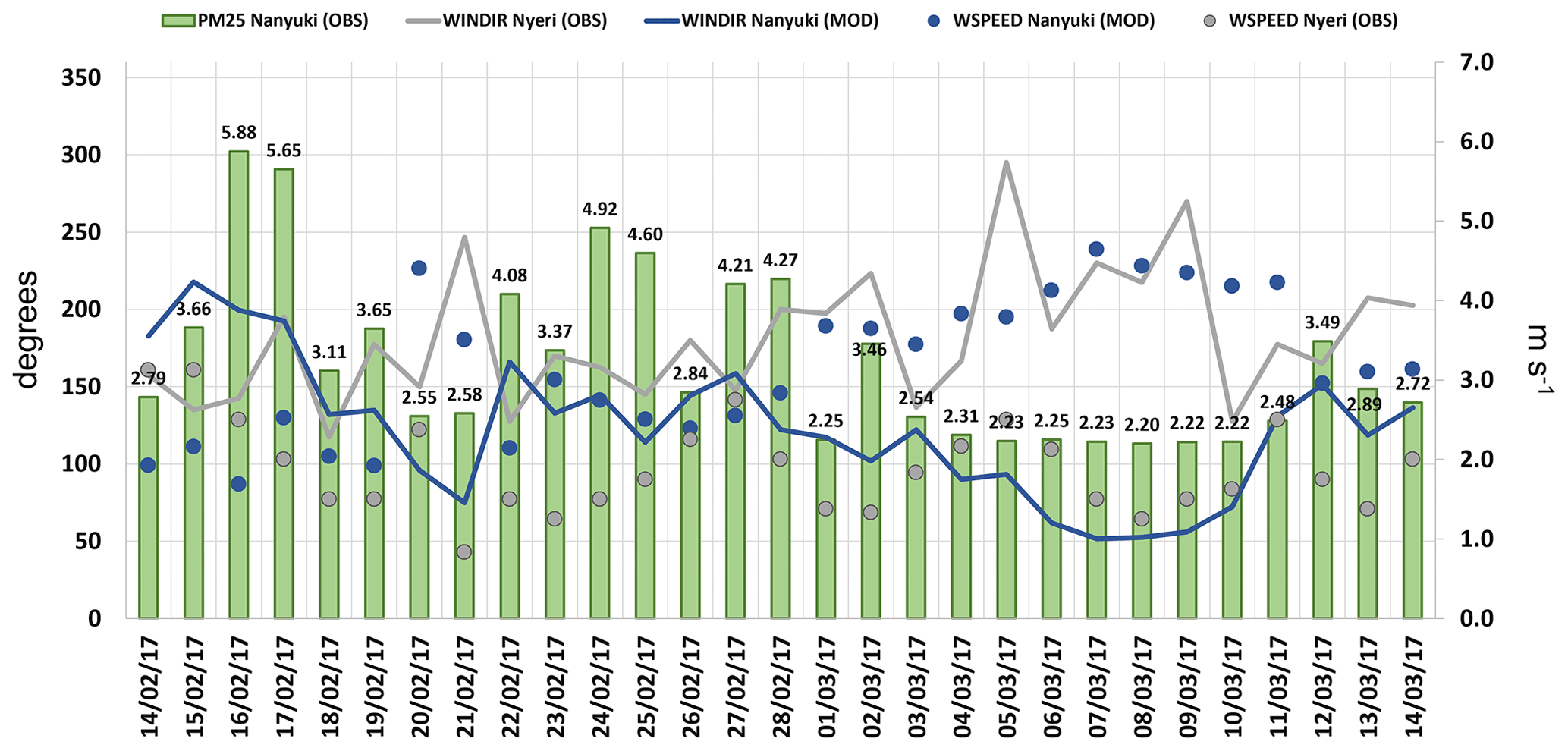
Figure 8 Comparison of daily observed values of wind speed (grey spots) and wind direction (grey lines) from the Nyeri MIDAS site (station no. 10 in Fig. 2c), modelled daily wind speed (blue dots), and wind direction (blue lines) from the Nanyuki site with daily average observations of PM_2.5 (expressed in µg m⁻³, green columns) obtained from the sampling site of Nanyuki (upper red dot in Fig. 2c).

In the periods with higher average daily concentrations of PM_2.5, namely between 15 and 19 February and between 22 and 28 February 2017, the component of wind direction seems to be consistent in reproducing southern winds (between 120 and 190^∘) in both Nyeri (using observations) and in Nanyuki (using model outputs) with wind speeds between 1.5 and 2.5 m s⁻¹ in the first period and between 2 and 3 m s⁻¹ in the second period.

The correspondence between the wind speed and direction during particular time periods and the vicinity of towns could suggest the potential dispersion of pollutants from the south, where the hotspot of Nyeri is located (upwind), to the northern area of Nanyuki (downwind), in accordance with the wind fluxes from south to north (from Nyeri) based on the observations and WRF outputs extracted from the Nanyuki location. The flux could also be driven by the location of Nyeri, which is situated at the entrance of a basin between two mountain ranges. On the other hand, during the period of low concentrations between 4 and 10 March, high speed north-easterly winds (around 60^∘) were noted in Nanyuki (around 4 m s⁻¹), whereas lower-speed winds (between 1 and 2 m s⁻¹) from more variable directions (between 170 and 300^∘) were present in Nyeri, preventing the possible dispersion of pollutants.

The present analysis was done on the relationships between weather conditions and their relative correspondence to the hourly and daily levels of PM_2.5. Further analyses are necessary to clarify the possible presence of additional or alternative factors influencing the changes in observed concentrations and concentrations modelled by CHIMERE. The presence of possible precipitation events during the low-concentration period could represent an alternative possible reason for the change in concentrations; however, no precipitation was recorded during the period, according to Pope et al. (2018), nor was any precipitation modelled by WRF in that time period. Nevertheless, the lack of additional weather observations at the sampling site of Nanyuki or midway between the two towns prevents any additional hypotheses from being formulated in relation to the presence of possible pollutant transport phenomena; this will be the subject of future investigations. Further efforts will be oriented toward a more detailed trajectory analysis of the winds as well as a more detailed representation of the emission sources present in the area in order to investigate possible transport effects in this region.

The average PM_2.5 concentrations for the entire simulation period (between 14 February and 14 March 2017) are shown for the domain centred over Kenya with a spatial resolution of 2 × 2 km (KEN2K; Fig. 9). The highest average concentrations during the monthly period are modelled in the urban area of Nairobi (defined by the red dashed square in Fig. 9), with the highest average values inside the city being around 80 µg m⁻³. The concentrations are spread, on average, in the southwestern area of the city and on the northeastern side of the city in the direction of the conurbation of Thika and Makuyu. These towns became part of the Nairobi metropolitan region in 2008 due to the rapid increase in population and urbanisation of the area (UNEP, 2009), and they represent a large hotspot of PM_2.5 emissions, with concentrations modelled between 20 and 30 µg m⁻³ on average over the entire period. Other PM_2.5 concentration hotspots found in the domain are the city of Nakuru, with average concentrations of between 20 and 40 µg m⁻³, and the area between Nyeri, Embu, Meru, and Siakago, with average concentrations of around 20 and 30 µg m⁻³ (Fig. 9). The average of the modelled concentrations in the area of Nanyuki is generally smaller, with the concentration not exceeding 10 µg m⁻³ over the whole area.

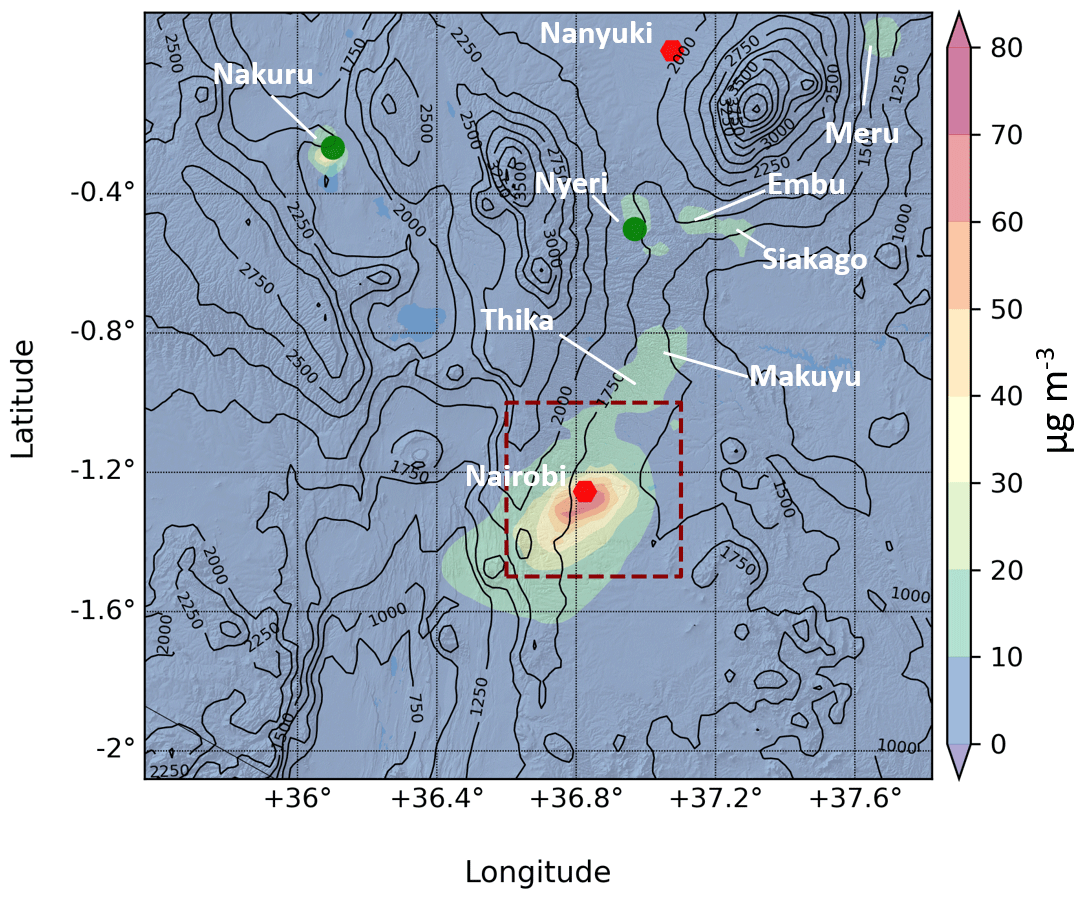
Figure 9 The average PM_2.5 concentration for the whole simulated period for the KEN2K domain at a 2 × 2 km spatial resolution. The map shows the location of hotspots with higher average concentrations, as modelled by CHIMERE, for the entire period. The red dashed square shows the urban domain of Nairobi analysed for the Air Quality Index analysis in Sect. 3.3.

3.3 CHIMERE as an air quality management tool

The usefulness of CHIMERE as a decision support tool to facilitate air quality management of large urban conurbations in SSEA was investigated for the three domains, namely KEN2K, UGA2K, and ETH2K, at a resolution of 2 × 2 km. Daily observations of PM_2.5 for the three domains were compared with modelled concentrations in terms of the number of exceedances of the WHO limit of 25 µg m⁻³ that were observed and captured by the model (Fig. 10). For the limited case of Nairobi, hourly average concentrations for the whole monitored period were compared with Air Quality Index data, and the spatial distribution of daily average concentrations in the constituencies was analysed, highlighting how many areas of the city showed poor Air Quality Index values during the analysed period (Fig. 11).

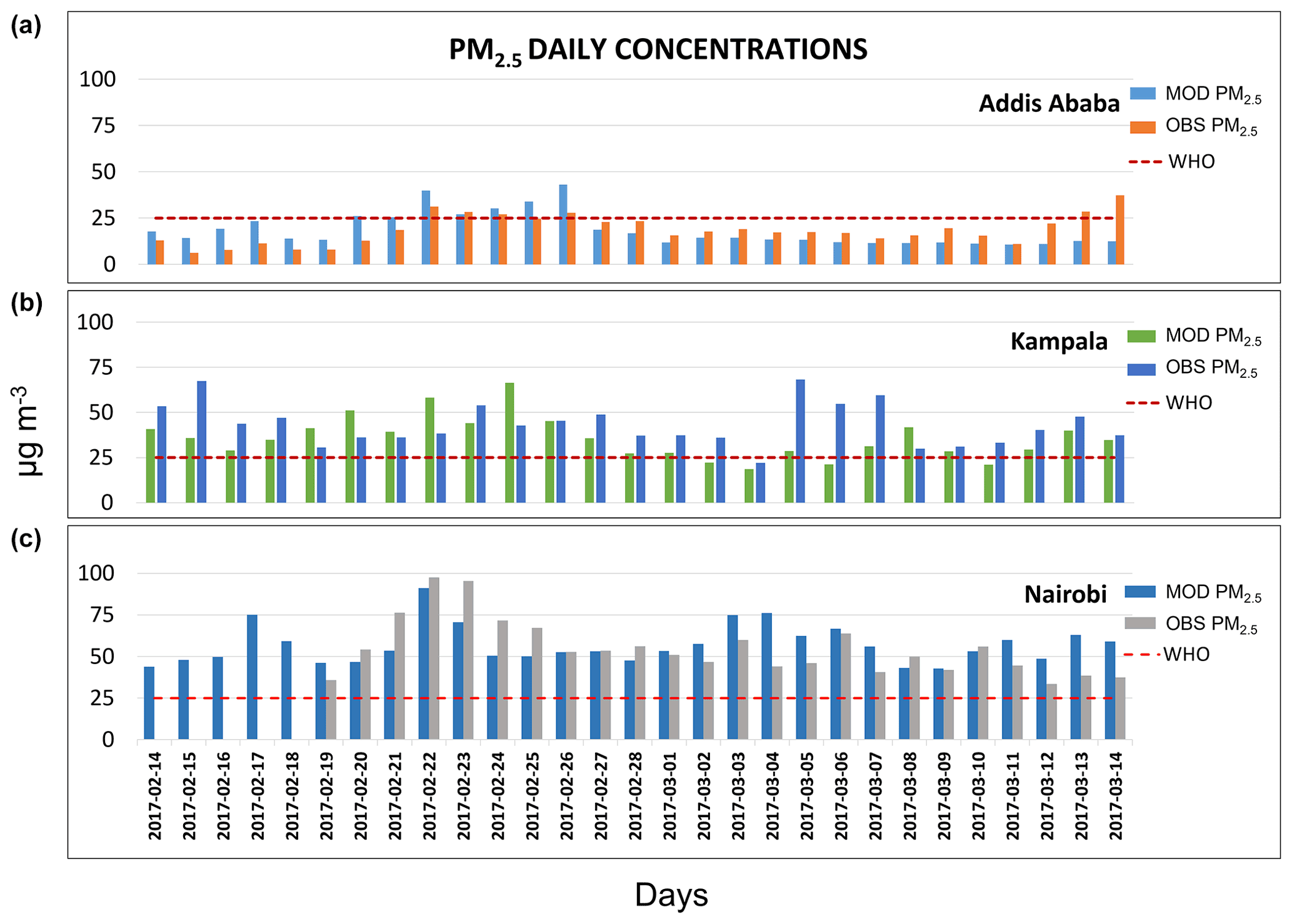
Figure 10 Daily concentrations of PM_2.5 between 14 February and 14 March obtained from CHIMERE outputs from 2 × 2 km domains compared with US embassy daily totals for the cities of (a) Addis Ababa and (b) Kampala and with ASAP observations for the city of (c) Nairobi. All three simulations have also been compared with the WHO threshold limit for PM_2.5 concentrations (red line). For the case of Nairobi, only observations from 18 February were available.

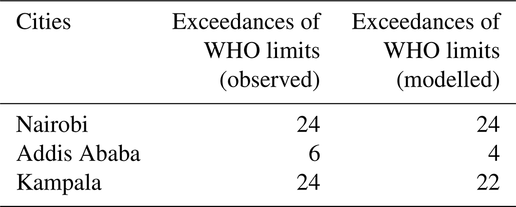
Daily concentrations of PM_2.5 modelled by CHIMERE were compared with the number of exceedances of the WHO limit of 25 µg m⁻³ observed during the simulated period. Figure 10 shows the daily average concentrations for the three cities at the sampling sites used for model validation. It can be seen that Nairobi and Kampala have the highest number of exceedances of the WHO limits (24), followed by Addis Ababa with only six observed exceedances. From Table 6, it can be seen that CHIMERE provides sufficient accuracy to detect PM_2.5 exceedances of the WHO limits. In particular, CHIMERE was able to detect 67 % of the exceedance for Addis Ababa with only two false positives, 91 % of the exceedance for Kampala, and all of the exceedances for Nairobi without any false positives.

The Air Quality Index (AQI) represents the conversion of concentrations for fine particles, such as PM_2.5, to a number on a scale from 0 to 500 (Table 6). The higher the AQI value, the greater the level of air pollution and the greater the health concern. AQI values at or below 100 are generally thought of as satisfactory. When AQI values are above 100, air quality is unhealthy – at first for certain sensitive groups of people (101–150) and then for everyone as AQI values get higher (> 151) (EPA, 2012).

Table 6 Summary of the number of observed and modelled PM_2.5 exceedances of the WHO limits during the simulated period from 14 February to 14 March 2017.

The daily average concentrations of PM_2.5 during the analysis period (between 14 February and 14 March 2017) have been averaged for the urban area of Nairobi (red square in Figs. 9 and 11) and compared with the city constituencies' spatial extent according to data from the openAFRICA data set (openAFRICA, 2018). According to the division, 17 are constituencies inside the Nairobi city boundaries (Fig. 11). Averaged daily concentrations of PM_2.5 show that 8 of the 17 constituencies had AQI values between 55.5 and 150.4 µg m⁻³ during the whole period. These areas are the most central and urbanised of Nairobi. Starehe constituency (station no. 13 in Fig. 11) contains the previously discussed Tom Mboya Street sampling site (black spot in Fig. 11) where the WHO limits for PM_2.5 were systematically exceeded during the analysed period. According to the SEDAC population density data, this area has a population density of between 15 000 and 30 000 people per square kilometre that are exposed to an AQI of between 151 and 200, corresponding to the “Unhealthy” category with respect to human health. Finally, the Langata constituency (magenta spot in Fig. 11) has a population of 176 000 people and shows average PM_2.5 levels of 45 µg m⁻³, which is unhealthy for sensitive groups of people.

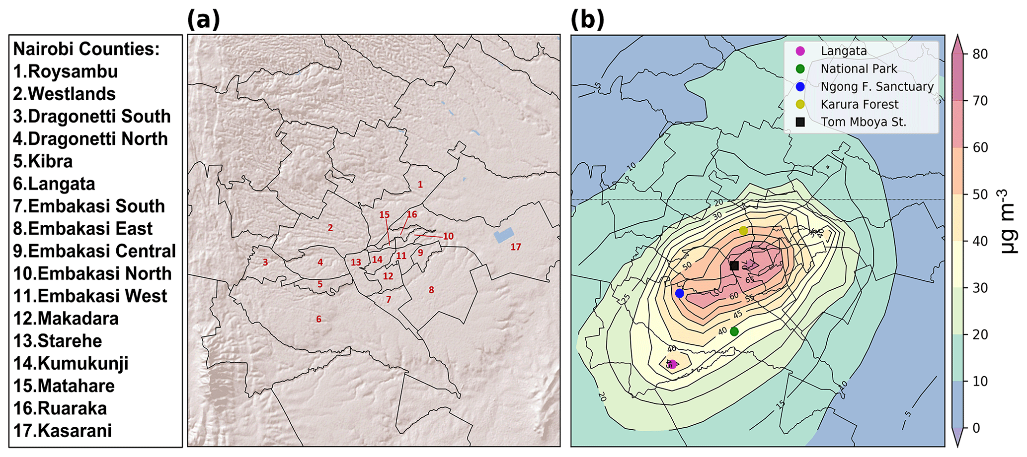
Figure 11 Map showing the urban area of the city of Nairobi (dashed square in Fig. 9). The constituency division of Nairobi in panel (a) from the openAFRICA data set (openAFRICA, 2018) is compared with the average hourly concentrations of PM_2.5 over the analysed period in panel (b).

Moreover, Nairobi has a number of natural areas on the outskirts of city. Some particular locations, such as the Karura Forest (yellow spot in Fig. 11) and the Ngong Road Forest Sanctuary (blue spot in Fig. 11), show averaged daily PM_2.5 levels of around 50 and 55 µg m⁻³, corresponding to an AQI of between 101 and 150 (e.g. unhealthy for certain sensitive groups of people). According to SEDAC data, the population density is between 10 000 and 15 000 people per square kilometre in this area. Similarly, on the south side, near the entrance to the Nairobi National Park (1.36^∘ S, 36.82^∘ E; green spot in Fig. 11), the average daily levels of PM_2.5 are approximately 40 µg m⁻³, with AQI values between 101 and 150 and a population density of around 10 000 people per square kilometre. This area (surface area of 117 km²) has been impacted by a rapid urbanisation since 1973, with a consequent increase in human activity including settlement, pastoralism, and agriculture (Ogega and Mbugua, 2019). This activity has already made it difficult for wildlife to migrate to and from the Nairobi National Park as well as resulting in a deterioration of air quality. The rapid increase in the population density on the south side of Nairobi poses a serious risk of increasing the pollution level or AQI, thereby exposing more people to a harmful level of PM_2.5.

4 Conclusions

The WRF and CHIMERE models were configured and validated to simulate the PM air quality levels in eastern sub-Saharan African urban conurbations.

In order to obtain updated anthropogenic emissions for 2017, the global EDGAR inventory and the DICE inventory for Africa were merged and spatially distributed using population density data for the year 2017 obtained by linear extrapolation.

WRF showed a variable capability with respect to reproducing the main surface weather variables according to the different conditions of the three domains. A lower agreement between observations and the model was observed in Kampala for relative humidity and wind speed. The analysis was carried out on all surface meteorological stations available from the MIDAS network on a 3-hourly basis. A further meteorological analysis extended to vertical profiles could reveal the possible limitations of the model; however, the absence of vertical meteorological data limited the analysis and validation to ground level only.

CHIMERE was able to reproduce the daily levels of PM_2.5 for the urban site of Nairobi as well as for the rural site of Nanyuki. A total of 69 % of the MFB values and 88 % of the MFE values were inside the highest confidence area for Nairobi, and a total of 97 % and 99 % of the respective values were inside the highest confidence area for Nanyuki, attesting that the agreement between the observed and modelled data was sufficient to allow for quantitative analyses of daily average concentrations. Similar findings were also produced for the other two urban background domains of Addis Ababa (57 % for MFB and 80 % for MFE) and Kampala (48 % for MFB and 74 % for MFE), despite different characteristics and sources of observation being used for the validation. The discrepancies observed in the hourly trends of PM_2.5 modelled by CHIMERE compared to observed values from the urban sites suggest that further studies are needed in the three urban areas. These studies are required to improve the understanding of the typology and quantity of local emission sources, which are sometimes misrepresented or absent in global emission inventories. This will enable the chemical processes acting in the urban troposphere to be adequately characterised, thereby allowing the determination of the actual air quality levels.

Nevertheless, using existing data sets, CHIMERE has shown reliability with respect to reproducing both hourly and daily levels of PM_2.5, with hourly values largely inside the range of reliability connected with the mean fractional bias and error.

The merged emission inventory, DICE–EDGAR, despite its low resolution, was able to return a correct magnitude for the emissions regarding the representation of the urban and rural contexts. Despite this, a few urban peaks observed in Nairobi have been missed by CHIMERE or, in other cases, misrepresented, highlighting the necessity of further efforts in the creation of newer emission inventories for SSEA. In the light of this, the possibility to develop local emission inventories, ideally at high spatial resolution, would represent a significant step forward in air quality research in this area of the world. Nevertheless, with the extent of the present available data, CHIMERE showed enough robustness and reliability to be adopted as a decision support tool for the management of air quality, as it correctly reproduced most of the exceedances of the PM_2.5 limits set by the WHO for all three cities considered.

The analysis focused on the average concentrations of PM_2.5 for the domain of Kenya revealed that the metropolitan area of Nairobi represents a big air pollution hotspot; however, it also showed that small cities located on the outskirts of the capital of Kenya display worrying levels of atmospheric contamination. These levels of air pollution have the potential capability to also affect rural areas where local emissions are rare or not present. The phenomena of PM_2.5 transport towards these areas, however, is still to be verified. The work has also shown the presence of low and unhealthy Air Quality Index values in 8 of the 17 constituencies in the urban area of Nairobi as well as the relative population density exposed to harmful level of air contamination. Moreover, a number of natural areas on the outskirts of Nairobi have similarly low AQI levels and an increasing population, highlighting how the problem of poor urban air quality due to rapid urbanisation, anthropogenic activity, and a lack of regulation can also detrimentally affect and deteriorate natural habitats.

The present work represents a first step in the use of numerical models for atmospheric chemistry simulations in East Africa with a particular focus on urban conurbations. The aim of this study was to assess the possibility of performing simulations with results that are close to observations in order to open the road for more detailed works. The natural next step of the present research aims to refine both the quantity and quality of the input data used for the validation of the modelling system in order to improve the reliability of the predictions. Moreover, a more detailed analysis of the secondary inorganic and organic components of PM_2.5 will be conducted for the three domains. Finally, the performance of CHIMERE will also be tested with respect to the reproduction of gaseous species in order to give a wider vision of the capabilities and opportunities of numerical modelling in this area of the world with the presently available data. Additional future efforts to improve the calibration and validation of the modelling system, especially relating to meteorology, will focus on assessing the dispersion dynamics of contaminants through urban centres and possible pollution transport events from urban to rural areas. To this end, further work is required by local East African authorities and research bodies to improve the quantity and the quality of data for weather and air quality simulations. However, in this work, we have shown that currently available data are sufficient to carry out simulations of air quality that can be used for the quantitative evaluation of the anthropogenic emissions impact and to support mitigation policies at the local level.