Atmospheric impacts of chlorinated very short-lived substances over the recent past – Part 1: Stratospheric chlorine budget and the role of transport

Impacts of chlorinated very short-lived substances (Cl-VSLS) on stratospheric chlorine budget over the first two decades of the 21st century are assessed using the Met Office’s Unified Model coupled to the United Kingdom Chemistry and Aerosol (UM-UKCA) chemistry–climate model; this constitutes the most up-to-date assessment and the first study to simulate Cl-VSLS impacts using a whole atmosphere chemistry–climate model. We examine the Cl-VSLS responses using a small ensemble of free-running simulations and two pairs of integrations where the meteorology was “nudged” to either ERA5 or ERA-Interim reanalysis.

The stratospheric chlorine source gas injection due to Cl-VSLS estimated from the free-running integrations doubled from ∼40 ppt Cl injected into the stratosphere in 2000 to ∼80 ppt Cl injected in 2019. Combined with chlorine product gas injection, the integrations showed a total of ∼130 ppt Cl injected into the stratosphere in 2019 due to Cl-VSLS. The use of the nudged model significantly increased the abundance of Cl-VSLS simulated in the lower stratosphere relative to the free-running model. Averaged over 2010–2018, simulations nudged to ERAI-Interim and ERA5 showed 20 ppt (i.e. a factor of 2) and 10 ppt (i.e. ∼50 %) more Cl, respectively, in the tropical lower stratosphere at 20 km in the form of Cl-VSLS source gases compared to the free-running case. These differences can be explained by the corresponding differences in the speed of the large-scale circulation. The results illustrate the strong dependence of the simulated stratospheric Cl-VSLS levels on the model dynamical fields. In UM-UKCA, this corresponds to the choice between free-running versus nudged set-up, and to the reanalysis dataset used for nudging.

Temporal changes in Cl-VSLS are found to have significantly impacted recent HCl and COCl₂ trends in the model. In the tropical lower stratosphere, the inclusion of Cl-VSLS reduced the magnitude of the negative HCl and COCl₂ trends (e.g. from $\sim -\mathrm{8}\mathit{\%}$(HCl)/decade and $\sim -\mathrm{4}$ ppt(COCl₂)/decade at ∼20 km to $\sim -\mathrm{6}\mathit{\%}$(HCl)/decade and ∼ −2 ppt(COCl₂)/decade in the free running simulations) and gave rise to positive tropospheric trends in both tracers. In the tropics, both the free-running and nudged integrations with Cl-VSLS included compared much better to the observed trends from the ACE-FTS satellite record than the analogous simulations without Cl-VSLS. Since observed HCl trends provide information on the evolution of total stratospheric chlorine and, thus, the effectiveness of the Montreal Protocol, our results demonstrate that Cl-VSLS are a confounding factor in the interpretation of such data and should be factored into future analysis. Unlike the nudged model runs, the ensemble mean free-running integrations did not reproduce the hemispheric asymmetry in the observed mid-latitude HCl and COCl₂ trends related to short-term dynamical variability. The individual ensemble members also showed a considerable spread of the diagnosed tracer trends, illustrating the role of natural interannual variability in modulating the diagnosed responses and the need for caution when interpreting both model and observed tracer trends derived over a relatively short time period.

1 Introduction

Stratospheric ozone plays a crucial role in shielding the Earth's surface from harmful UV radiation. Its absorption of shortwave radiation also plays a crucial role in modulating stratospheric temperatures which can feed back on atmospheric transport and influence surface climate (e.g. Nowack et al., 2015). The absorption of longwave radiation by ozone in the troposphere and lower stratosphere, on the other hand, contributes to the greenhouse effect. The important role of halogens in modulating stratospheric ozone levels is now well understood (e.g. WMO, 2018). To date, most attention has been given to long-lived chlorinated and brominated ozone depleting substances (ODSs), of which significant past emissions have been the principal cause of stratospheric ozone depletion with subsequent impacts on levels of surface UV (e.g. Bais et al., 2018) and surface climate (e.g. Son et al., 2009).

Another class of halogenated compounds that are also thought to contribute to stratospheric ozone depletion are very short-lived substances (VSLS). These gases have atmospheric lifetimes near the surface of less than about six months and, hence, are not well mixed in the troposphere (e.g. Engel et al., 2018). In the past two decades, a wealth of research has examined the sources and sinks of brominated VSLS (e.g. bromoform, CHBr₃) of predominantly oceanic origin (e.g. Sturges et al., 2000; Quack and Wallace, 2003) along with their contribution to stratospheric bromine and impact on ozone (e.g. Hossaini et al., 2016a; Oman et al., 2016; Wales et al., 2018; Keber et al., 2020). However, comparatively few studies have considered the atmospheric impacts of chlorinated VSLS (Cl-VSLS), which have significant anthropogenic sources and include dichloromethane (CH₂Cl₂), chloroform (CHCl₃), perchloroethylene (C₂Cl₄) and ethylene dichloride (C₂H₄Cl₂), among others. There is strong evidence that Cl-VSLS can enter the stratosphere, thereby affecting stratospheric ozone, based on measurements of the above compounds and their products in the upper troposphere/lower stratosphere (UTLS) region and modelling (e.g. Laube et al., 2008; Leedham Elvidge et al., 2015; Oram et al., 2017; Harrison et al., 2019; Hossaini et al., 2019).

The sources of Cl-VSLS were recently reviewed by Chipperfield et al. (2020). Briefly, CH₂Cl₂ is used in a range of emissive applications (e.g. as a solvent for paint stripping) and as a feedstock in the production of HFC-32 (Feng et al., 2018). Global total CH₂Cl₂ emissions of ∼1 Tg yr⁻¹ have been inferred for 2017 from inversion analysis of atmospheric observations, with Asian emissions increasing markedly over the recent period (Feng et al., 2018; Claxton et al., 2020). For CHCl₃, its industrial use is principally as a feedstock for HCFC-22 production which itself has a range of both emissive and non-emissive uses. Global total CHCl₃ emissions of 324 Gg yr⁻¹ in 2015 were inferred from inverse modelling, with emissions from China suggested as the dominant source location (Fang et al., 2019).

Past and future changes in stratospheric ozone continue to be the subject of multi-model assessment studies (e.g. Dhomse et al., 2018) employing chemistry–climate models (CCMs). However, none of the CCMs participating in such studies, to our knowledge, has so far included Cl-VSLS thereby omitting a process of potential direct importance to the simulated ozone fields. Past studies examining the atmospheric impacts of Cl-VSLS have employed offline stratospheric chemistry–transport models (CTM) driven by meteorological reanalysis (e.g. Hossaini et al., 2015, 2019; Claxton et al., 2020). While being able to accurately represent the background interannual dynamical variability, the use of prescribed meteorology meant those studies were unable to simulate the radiative feedback of ozone and ozone changes on the underlying stratospheric temperatures and circulation.

In this study, we assess the atmospheric impacts of Cl-VSLS using the Met Office's Unified Model coupled to the United Kingdom Chemistry and Aerosol (UM-UKCA) CCM. The study is divided into three parts constituting the most up-to-date end-to-end assessment of the Cl-VSLS impacts. Part 1 here assesses the atmospheric signatures of Cl-VSLS using a small ensemble of free-running integrations over 2000–2019. The focus is on quantifying the stratospheric input of Cl-VSLS and its impacts on HCl and COCl₂ trends; the latter are important proxies for inferring changes in total stratospheric chlorine content and, thus, aiding the monitoring of the effectiveness of the Montreal Protocol. We complement these free-running simulations with integrations where the model meteorology was “nudged” towards the observed conditions as given by two different reanalysis datasets. This comparison between the free-running and nudged approaches provides insight into and demonstrates the role of atmospheric dynamics and model dynamical fields in modulating the atmospheric responses to Cl-VSLS. It also demonstrates the importance of the choice of model set-up in UM-UKCA for the inferred responses.

Section 2 of this paper (Part 1) describes the UM-UKCA model and the simulations performed. Section 3 quantifies the stratospheric input of Cl-VSLS and the resulting impacts on stratospheric chlorine species. Section 4 focuses on the impacts of Cl-VSLS on the recent HCl trends and Sect. 5 on the recent COCl₂ trends. Our main results are summarised and discussed in Sect. 6. In the follow up to this work, we will focus on the impacts of Cl-VSLS on stratospheric ozone (Part 2) and compare simulations forced with lower boundary conditions of Cl-VSLS, as used here, with simulations using recently estimated Cl-VSLS emissions from Claxton et al. (2020) (Part 3).

2 Methods

2.1 Model description

We use version 11.0 of the UM-UKCA CCM, the atmosphere-only configuration of the UKESM1 Earth system model (Sellar et al., 2019). The full description of the model can be found in Sellar et al. (2019) and Archibald et al. (2020). Briefly, the model consists of the Global Atmosphere 7.1 configuration of the version 3 of the Hadley Centre Global Environment Model (GA7.1 HadGEM3, Walters et al., 2019) coupled to the UKCA chemistry and aerosol module (Morgenstern et al., 2009). The horizontal resolution is 1.875^∘ longitude $\times \mathrm{1.75}{}^{\circ }$ latitude, with 85 vertical levels up to ∼84 km on terrain-following hybrid height coordinate.

We use a newly developed “Double Extended Stratospheric-Tropospheric Scheme” (DEST, Bednarz et al., 2022). The scheme constitutes an extension of the standard StratTrop scheme described in Archibald et al. (2020). It includes an explicit treatment of 14 long-lived ODSs (CFC-11, CFC-12, CFC-113, CFC-114, CFC-115, CH₃Cl, CCl₄, CH₃CCl₃, HCFC-22, HCFC-141b, HCFC-142b, CH₃Br, Halon-1211 and Halon-1301) and some of the most important chlorinated (CH₂Cl₂, CHCl₃, C₂Cl₄ and C₂H₄Cl₂) and brominated (CHBr₃, CH₂Br₂CH₂BrCl, CHBr₂Cl and CHBrCl₂) VSLS. The long-lived ODSs are forced at the surface using global mean time-varying lower boundary conditions (LBCs). The Cl-VSLS tracers are forced at the surface using latitudinally and time-varying LBCs (see below), and the climatological emissions of the predominately natural Br-VSLS are used following Ordóñez et al. (2012). A detailed description and evaluation of the scheme can be found in Bednarz et al. (2022).

Table 1 Summary of UM-UKCA integrations performed.

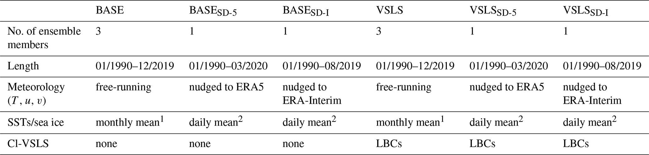
¹ Durack and Taylor (2016) over 1990–2016, and Reynolds and Smith (1994) over 2017–2019. ² Reynolds and Smith (1994).

2.2 Model experiments

A set of UM-UKCA transient integrations was performed over the period 1990–2019. Observed sea-surface temperatures (SSTs) and sea ice are prescribed in all runs. For the free-running integrations, we use the Coupled Model Intercomparison Project Phase 6 (CMIP6)-recommended dataset described in Durack and Taylor (2016) until 2016, and the Reynolds and Smith (1994) dataset, monthly-averaged, thereafter. In all simulations, surface concentrations of greenhouse gases and the long-lived ODSs follow Meinshausen et al. (2017) from 1990 to 2014, and then the CMIP6 Shared Socioeconomical Pathway SSP2-4.5 scenario (Meinshausen et al., 2020) from 2015 to 2019. Emissions of aerosols and chemical tracers of importance in the troposphere are as in Archibald et al. (2020) and Sellar et al. (2020) until 2014, and then follow SSP2-4.5. Surface area density of stratospheric sulfate aerosols is from Thomason et al. (2018) until 2014 and climatological thereafter. In all experiments (summarised in Table 1), the period from 1990 to 1999 is treated as a model “spin-up” and so only model output from 2000 onwards is analysed.

A three-member ensemble of free-running integrations was carried out without Cl-VSLS. We denote this ensemble as “BASE”. The experiment spans the period from January 1990 to December 2019 inclusive. A second three-member ensemble of free-running integrations, denoted “VSLS”, is analogous to BASE but includes four of the most important Cl-VSLS (CH₂Cl₂, CHCl₃, C₂Cl₄ and C₂H₄Cl₂) constrained at the surface using latitude- and time-dependent LBCs. For each Cl-VSLS, the surface LBCs are applied in the model in five latitude bands (90–30^∘ S, 30^∘ S–0, 0–30^∘ N, 30–60^∘ N and 60–90^∘ N) and vary annually. For a given year, the annual LBCs are calculated by averaging surface measurements from available sites within each of the five latitude bands. Based on our previous work (Hossaini et al., 2019), measurement data from the National Oceanic and Atmospheric Administration (NOAA) global monitoring network were used for CH₂Cl₂ and C₂Cl₄ while Advanced Global Atmospheric Gases Experiment (AGAGE) network data were used for CHCl₃. For C₂H₄Cl₂, latitude-dependent LBCs were estimated (see Hossaini et al., 2016b) based on measurements made during the 2009–2011 HIAPER Pole-to-Pole Observations (HIPPO) aircraft campaign (Wofsy, 2011). In the 1990–1999 period (i.e. spin-up), Cl-VSLS LBCs are assumed to be the same as for the year 2000. The time evolution of the global mean surface concentration of each Cl-VSLS is shown in Fig. 1, and the evolution in each of the five latitude bands is shown in Fig. S1 in the Supplement.

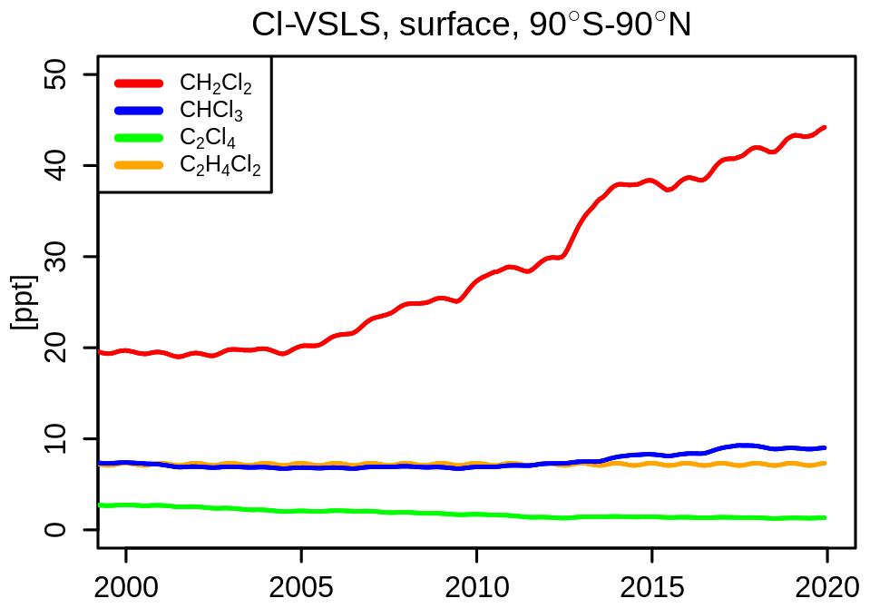
Figure 1 Global mean volume mixing ratios [ppt] of CH₂Cl₂ (red), CHCl₃ (blue), C₂Cl₄ (green) and C₂H₄Cl₂ (orange) simulated at the surface in the VSLS experiments.

The free-running BASE and VSLS model ensembles were complemented with two sets of similar integrations but using the specified dynamics configuration of UM-UKCA, i.e. in which model meteorology (in particular, temperature, zonal and meridional winds) are “nudged” towards observed conditions (Telford et al., 2008). These follow European Centre for Medium-Range Weather Forecasts (ECMWF) ERA5 reanalysis (Hersbach et al., 2020) in the first pair of integrations – VSLS_SD-5 and BASE_SD-5 – and the ECMWF ERA-Interim reanalysis (Dee et al., 2011) in the second pair – VSLS_SD-I and BASE_SD-I. The first pair covers the period until the end of March 2020 and the second pair, limited by the length of the ERA-Interim dataset, up to August 2019 inclusive. For better consistency with nudging frequency, rather that the monthly mean SSTs/sea-ice data used in the free-running integrations, we use the daily mean Reynold and Smith (1994) dataset throughout the simulation period. Comparison of the two datasets shows overall similar evolution of the monthly mean tropical SSTs (Fig. S2), thereby suggesting that any differences in the simulated responses between the free-running and nudged integrations are not primarily the result of the differences in the imposed SSTs. Note that in the subsequent discussion of Cl-VSLS impacts, for brevity, we refer to the difference between the ensemble mean free-running VSLS and BASE experiments as “ΔFR”; and to the difference between the nudged VSLS_SD-5 and BASE_SD-5 (or VSLS_SD-I and BASE_SD-I) as “ΔSD-5” (or “ΔSD-I”).

Figure 2 Annual mean zonal mean 2010–2019 volume mixing ratios [ppt] of (a) CH₂Cl₂, (b) CHCl₃, (c) C₂Cl₄, (d) C₂H₄Cl₂ and (e) Cl in Cl-VSLS source gases simulated in the ensemble mean VSLS experiment. Dashed line in (a–e) illustrates ensemble mean tropopause. Panel (f) shows the corresponding difference in total chlorine (Cl_tot) [ppt] between the ensemble mean VSLS and BASE (i.e. the ΔFR response); contours in (f) show Cl_tot [ppb] in the VSLS experiment for reference.

3 Stratospheric input of Cl-VSLS and impacts on stratospheric chlorine species

3.1 Free-running simulations

The simulated ensemble mean concentrations of different Cl-VSLS (averaged over the final decade of the VSLS runs, i.e. 2010–2019) are shown in Fig. 2. In accord with the latitudinal gradient in the prescribed Cl-VSLS LBCs (Fig. S1), the highest source gas concentrations occur in the Northern Hemisphere (NH) troposphere, decreasing in magnitude with increasing altitude due to atmospheric degradation processes. We model significant amounts of Cl-VSLS near the tropical tropopause amounting to ∼70 ppt Cl at 17 km (Fig. 2e). The stratospheric source gas injection (SGI) of chlorine from Cl-VSLS can be calculated based on their simulated concentrations at 17 km and 25^∘ S–25^∘ N, as shown in Fig. 3. We find that the simulated SGI doubled over the first two decades of the 21st century, with ∼80 ppt Cl being injected into the stratosphere in the form of Cl-VSLS in 2019 compared to ∼40 ppt Cl in 2000 (black line in Fig. 3b). Combined with the additional Cl reaching the stratosphere in the form of product gases (i.e. product gas injection, PGI), e.g. HCl, we find ∼130 ppt of extra Cl reaching the stratosphere in 2019 (compared to ∼70 ppt in 2000) due to Cl-VSLS alone (purple line in Fig. 3b).

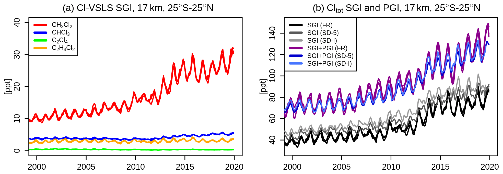
Figure 3 Monthly mean volume mixing ratios [ppt] at 25^∘ S–25^∘ N and 17 km for (a) CH₂Cl₂ (red), CHCl₃ (blue), C₂Cl₄ (green) and C₂H₄Cl₂ (orange) in the free-running VSLS experiment (individual ensemble members), and (b) Cl present in the Cl-VSLS (i.e. SGI, black) in the VSLS experiment (individual ensemble members), and the difference in Cl_tot between the VSLS ensemble members and the ensemble mean BASE (i.e. SGI+PGI, purple). Grey lines in (b) indicate SGI in the nudged VSLS_SD-5 and VSLS_SD-I runs, and blue lines the respective SGI+PGI.

We note that although the individual ensemble members in these free-running experiments have, by definition, different meteorology, the simulated stratospheric SGI and PGI of chlorine show very similar inter-annual variability (Fig. 3b). Recall that all three VSLS ensemble members are forced with identical chemical (i.e. Cl-VSLS) and oceanic (i.e. SSTs and sea ice) LBCs. Hence, the results suggest that it is the interannual differences in the Cl-VSLS surface mixing ratios and the SSTs (Fig. S2) and sea-ice data, rather than the model internal dynamical variability, that is the main driver of the variability in SGI and PGI on interannual timescales. We note that interannual variability in tropical SSTs in particular has been previously shown to be an important driver of variability in large-scale atmospheric circulation (e.g. Neu et al., 2014); this effect will thus likely play an important role for modulating the stratospheric Cl-VSLS transport.

The transport of Cl from Cl-VSLS into the stratosphere adds to the already elevated stratospheric chlorine levels caused by past emissions of long-lived ODSs. Averaged over the last decade (2010–2019), our simulations show ∼100 ppt of additional chlorine in the lower/mid-stratosphere in the VSLS experiment compared to BASE (Fig. 2f). This accounts for ∼3 % of total stratospheric chlorine for that period.

Figure 4 Shading: annual and zonal mean 2010–2019 difference [ppt] in (a) HCl, (b) ClONO₂, (c) COCl₂ and (d) ClO between the ensemble mean VSLS and BASE experiments (i.e. the ΔFR responses). Contours show the corresponding values in the ensemble mean VSLS for reference; note that contours in (a, b) are in ppb.

Figure 4 speciates the modelled difference in chlorine between the experiments VSLS and BASE. Most of the additional Cl in the former runs is found as HCl, the principal stratospheric chlorine reservoir, and in ClONO₂, ClO and COCl₂. The latter is an important product of Cl-VSLS oxidation and an atmospheric degradation product of the longer-lived source gases CCl₄ and CH₃CCl₃ (e.g. Fu et al., 2007; Harrison et al., 2019). Here, we estimate that up to 8 ppt of the COCl₂ simulated over the last decade in the VSLS experiment is of Cl-VSLS origin, with Cl-VSLS accounting for the majority of COCl₂ found in the troposphere. In terms of the contribution to the stratospheric chlorine injection from product gases (PGI), we find that averaged over 2010–2019 the inclusion of Cl-VSLS results in 27 ppt more Cl injected in the form of HCl and 12 ppt more Cl injected in the form of COCl₂ compared to BASE. This can be compared to the 66 ppt Cl injected as Cl-VSLS source gases on average over the same period. The increase in HCl abundance in the mid-/upper stratosphere brought about from the inclusion of Cl-VSLS LBCs and chemistry in the model reduces the underestimation of HCl in that region compared to satellite data (Bednarz et al., 2022).

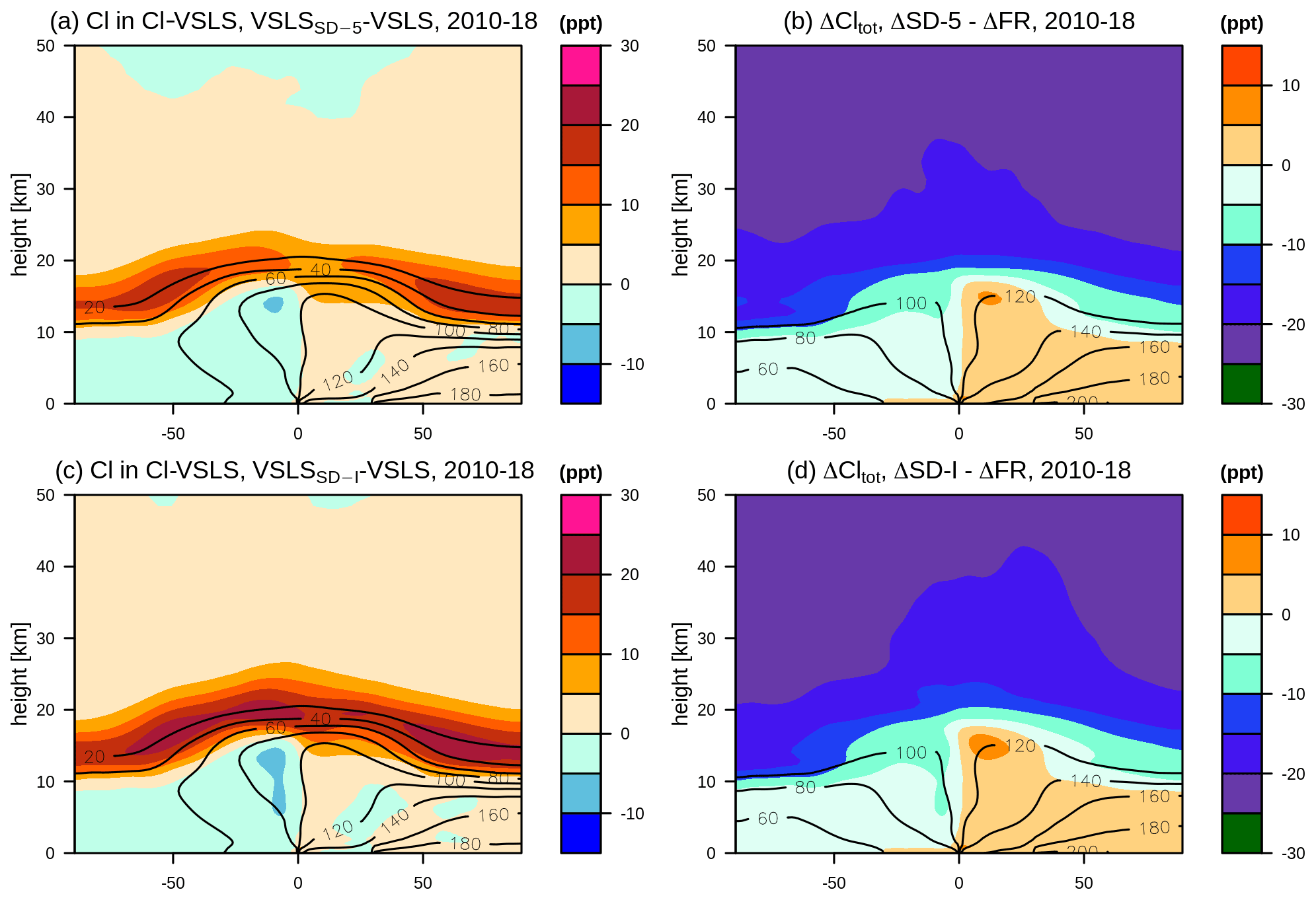
Figure 5 Shading: 2010-2018 difference in Cl [ppt] in (a, c) Cl-VSLS source gases between (a) VSLS_SD-5 and the ensemble mean VSLS, and between (c) VSLS_SD-I and the ensemble mean VSLS; (b, d) the difference between the Cl_tot responses in (b) ΔSD-5 and ΔFR and in (d) ΔSD-I and ΔFR. Contours show the corresponding values in the free-running VSLS for reference.

3.2 Free-running vs. nudged simulations

We now consider the sensitivity of the modelled stratospheric chlorine SGI and PGI to the choice between the free-running and nudged meteorology. We find that the use of the nudged model set-up in UM-UKCA significantly increases the abundance of Cl-VSLS in the lower stratosphere (Fig. 5a, c) and, hence, the stratospheric chlorine SGI from Cl-VSLS (Fig. 3a). For example, in the tropical (25^∘ S–25^∘ N mean) lower stratosphere at 20 km altitude, the nudged VSLS_SD-I run shows 20 ppt more Cl in the form of source gases relative to the free-running VSLS simulation (39 ppt and 19 ppt in VSLS_SD−I and VSLS, respectively, i.e. a factor of 2, averaged over 2010–2018; Fig. 5c). There is also a strong dependence on the reanalysis used for nudging, with the run nudged to ERA5 (VSLS_SD-5) showing 10 ppt more Cl in this region (29 and 19 ppt in VSLS_SD-5 and VSLS, respectively, i.e. ∼50 %) in the form of source gases than in the free-running experiments instead (Fig. 5a).

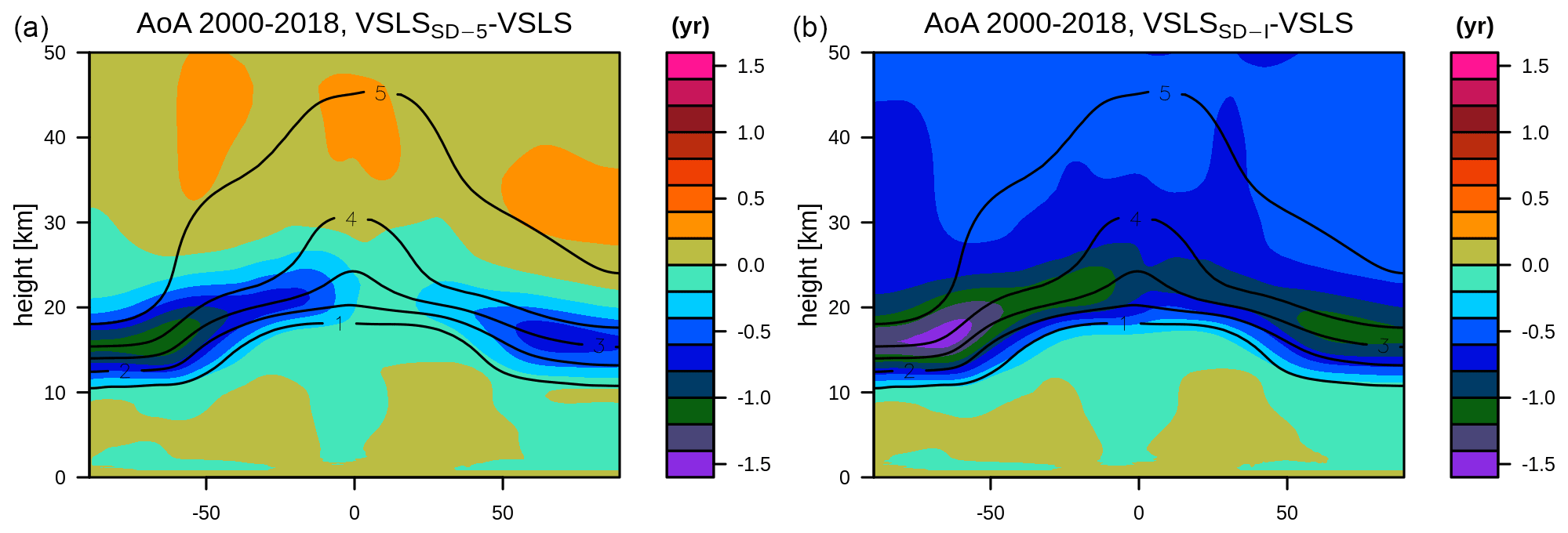
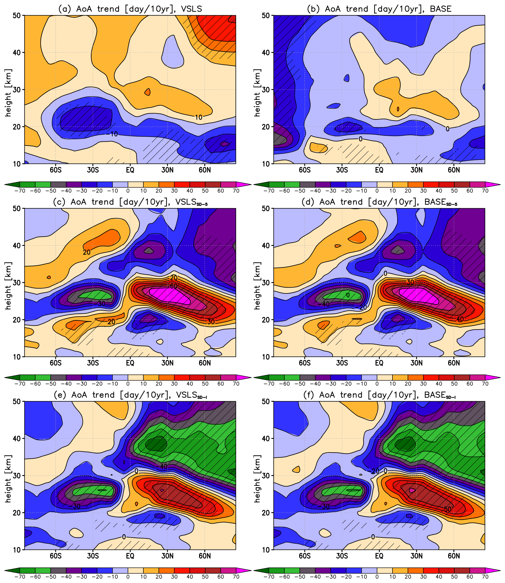
Figure 6 Shading: 2000–2018 difference in the model age-of-air [year] between the nudged and free-running integrations. (a) The difference between VSLS_SD-5 and the ensemble mean VSLS, and (b) the difference between VSLS_SD-I and the ensemble mean VSLS. Contours show the age-of-air in the ensemble mean free-running VSLS for reference.

These larger stratospheric concentrations of Cl-VSLS arise because of a markedly faster large-scale atmospheric circulation simulated in UM-UKCA in the nudged runs, particularly in the lower stratosphere (Fig. 6). The faster large-scale circulation accelerates the transport of Cl-VSLS across the tropical tropopause and into the lower stratosphere. Chrysanthou et al. (2019) found that an acceleration of tropical upwelling in nudged CCMs, compared to their free-running versions, is a common feature across different models. Here, the differences in the simulated age-of-air (AoA) between the nudged and free-running UM-UKCA simulations are larger for the run nudged to ERA-Interim than for the run nudged to ERA5. This corresponds to relatively slower Brewer–Dobson Circulation (BDC) in ERA5 compared to ERA-Interim, in agreement with previous studies (Diallo et al., 2021; Ploeger et al., 2021). The larger differences in transport between the free-running and ERA-Interim nudged UM-UKCA simulations are commensurate with larger difference in Cl-VSLS levels in the lower stratosphere.

Chrysanthou et al. (2019) analysed transport in CCMs and showed that while nudging does have a large impact on the resolved large-scale residual circulation in these models, it does not necessarily constrain its mean strength or otherwise improves it compared with the free-running models, similar to the conclusions of Orbe et al. (2018). The performance of the model stratospheric transport can be assessed by comparing the model AoA with that diagnosed from satellite observations of long-lived tracers. Here, Fig. 7 compares UM-UKCA AoA against the same quantity derived from the Michelson Interferometer for Passive Atmospheric Sounding (MIPAS) satellite observations of SF6 (Stiller et al., 2020). Note that both the model and the observed AoA were normalised by subtracting the values calculated in each case at the tropical tropopause. We find that in the tropics the stratospheric AoA in the run nudged to ERAI-Interim (VSLS_SD-I) compares more favourably to the MIPAS data than the AoA in the other simulations. However, this is not the case in the mid- and high latitudes. Therefore, rather than judging unambiguously which model set-up performs better, we highlight the importance this choice between the free-running and nudged configuration in UM-UKCA, alongside the choice of reanalysis dataset for the latter, has on the diagnosed Cl-VSLS response.

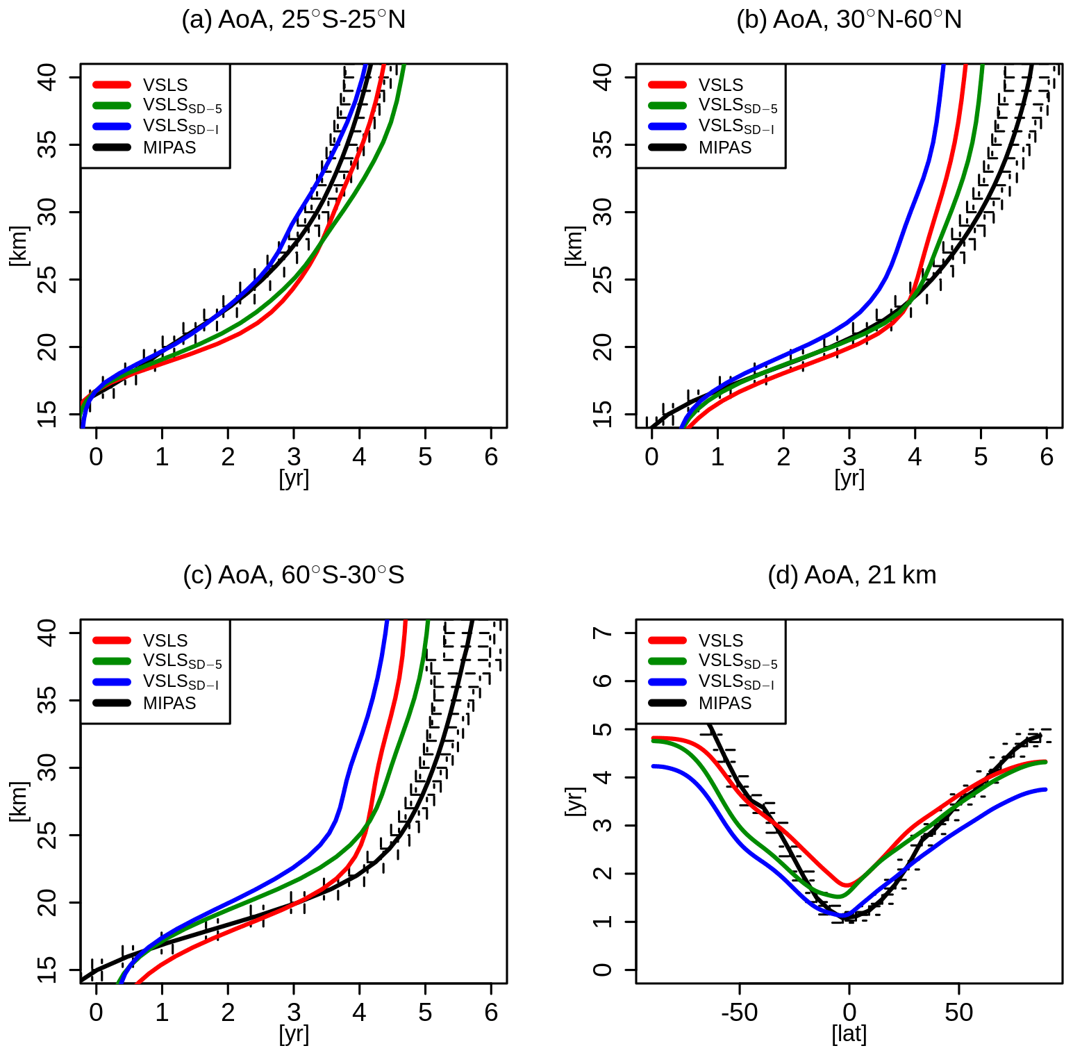
Figure 7 Normalised age-of-air [year] for (a) 25^∘ S–25^∘ N, (b) 30^∘ S–60^∘ N, (c) 30^∘ N–60^∘ S and (d) at 21 km, diagnosed from the free-running VSLS (red) and the nudged VSLS_SD-5 (green) and VSLS_SD-I (blue) simulations. Black shows the corresponding AoA derived from the MIPAS SF6 satellite observations (black; Stiller et al., 2020). Both model and observed AoA were averaged over the seven-year period from May 2005 to April 2012 inclusive. Both model and observed AoA were normalised to be zero at the tropical tropopause by subtracting the values calculated in each case for the tropical tropopause layer (here approximated as mean over 25^∘ S–25^∘ N, 16–17 km).

While the stratospheric concentrations of Cl-VSLS (and hence chlorine SGI) simulated in the nudged UM-UKCA runs are significantly larger than in the free-running runs, the corresponding changes in total stratospheric chlorine (Cl_tot) are slightly smaller for ΔSD-5 and ΔSD-I than for ΔFR (Fig. 5b, d). This corresponds to the relatively smaller increases in product gas injection in the nudged runs and, hence, in the relatively smaller increases in stratospheric concentrations of product gases (Figs. S3 and S4). This likely indicates (i) an enhanced transport of chlorine into the lower stratosphere in the form of Cl-VSLS rather than product gases (i.e. a higher SGI : PGI ratio), and (ii) an accelerated removal of inorganic chlorine from the stratosphere under faster large-scale circulation. In addition, changes in the washout efficiency of halogenated species (e.g. Fernandez et al., 2021) might also play a role.

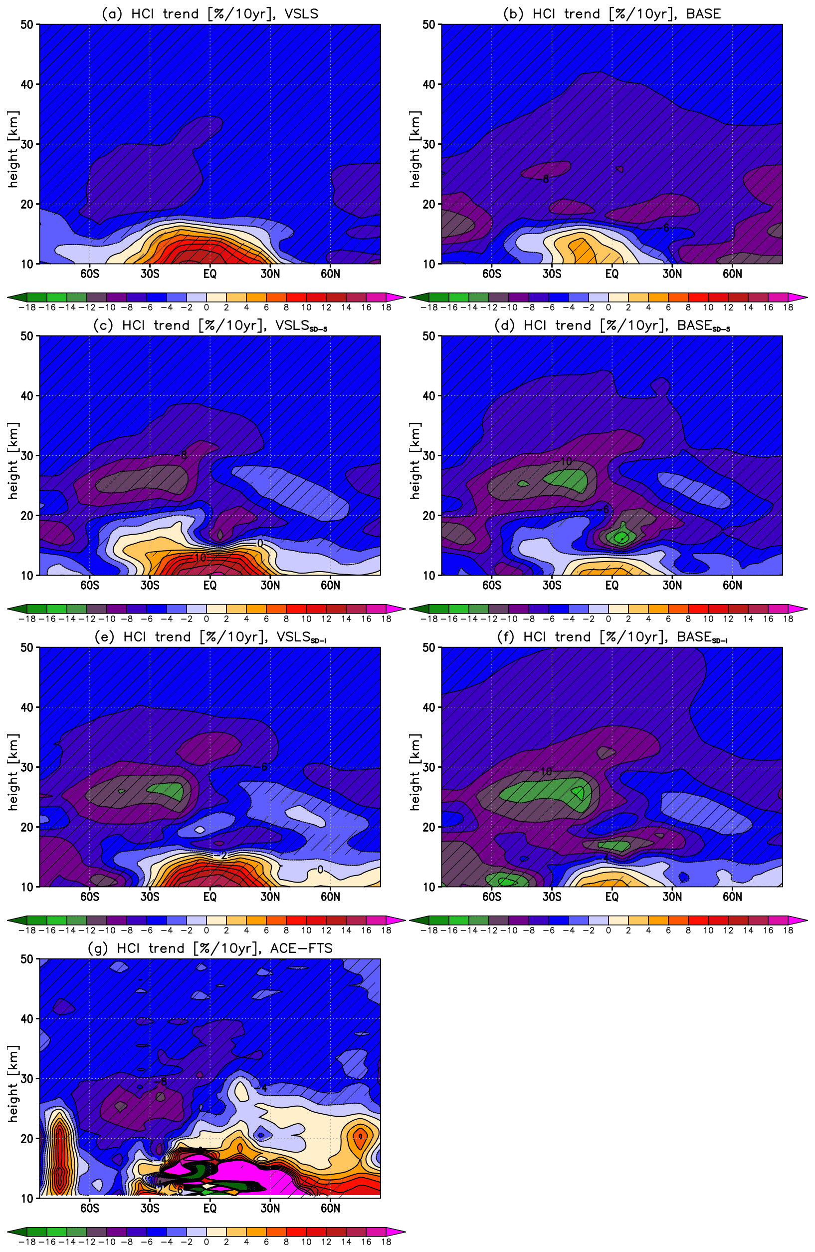
Figure 8 Linear trends in deseasonalised HCl mixing ratios [% per 10 years] in (a) the ensemble mean VSLS, (b) ensemble mean BASE, (c) the nudged VSLS_SD-5, (d) BASE_SD-5, (e) VSLS_SD-I, (f) BASE_SD-I, and from (g) the observed ACE-FTS satellite data (g). Trends in (a, b, c, d, g) are calculated over MAM2004–SON2019; trends in (e, f) are calculated over MAM2004–JJA2019. Hatching indicates statistical significance, here taken as regions where the magnitude of the derived trend exceeds ±2 standard errors.

4 The impacts of Cl-VSLS on HCl trends

4.1 Ensemble mean free-running simulations

Figure 8 shows linear trends in the deseasonalised HCl mixing ratios (MAM 2004–SON 2019) calculated from the free-running (ensemble mean) and nudged experiments. The trends are shown with and without Cl-VSLS, and as a function of latitude and height. The observed HCl trend derived from the Atmospheric Chemistry Experiment Fourier Transform Spectrometer (ACE-FTS, vn3.5-3.6) satellite data (Boone et al., 2013) is also shown for comparison. In each case, zonal and monthly mean HCl data were first interpolated onto a 10^∘-latitude grid and seasonally averaged (DJF, MAM, JJA and SON; all seasonal means calculated using data from the beginning of first month to the end of last month). The resulting seasonal mean time series was then deseasonalised (i.e. long-term mean for each season was removed), and a simple linear trend was calculated. Note that for the runs nudged to ERA-Interim (VSLS_SD-I, BASE_SD-I), the trends are calculated for a slightly shorter time period from MAM2004 to JJA2019 inclusive.

In general, stratospheric HCl mixing ratios have been decreasing since near the turn of the century, in line with the phase-out of long-lived ODSs and decreasing total stratospheric chlorine (Froidevaux et al., 2015; Bernath and Fernando, 2018). In accord, our BASE experiment shows a negative HCl trend that maximises in the tropical lower stratosphere at $\sim -\mathrm{8}$ %/decade at ∼20 km altitude (Fig. 8b). There is also a small positive HCl trend in BASE in the tropical upper troposphere (up to ∼4 %/decade at 10 km); this positive HCl trend is consistent in terms of the sign with the positive, albeit not statistically significant, tropospheric HCl trend inferred from the ACE-FTS data (Fig. 8g).

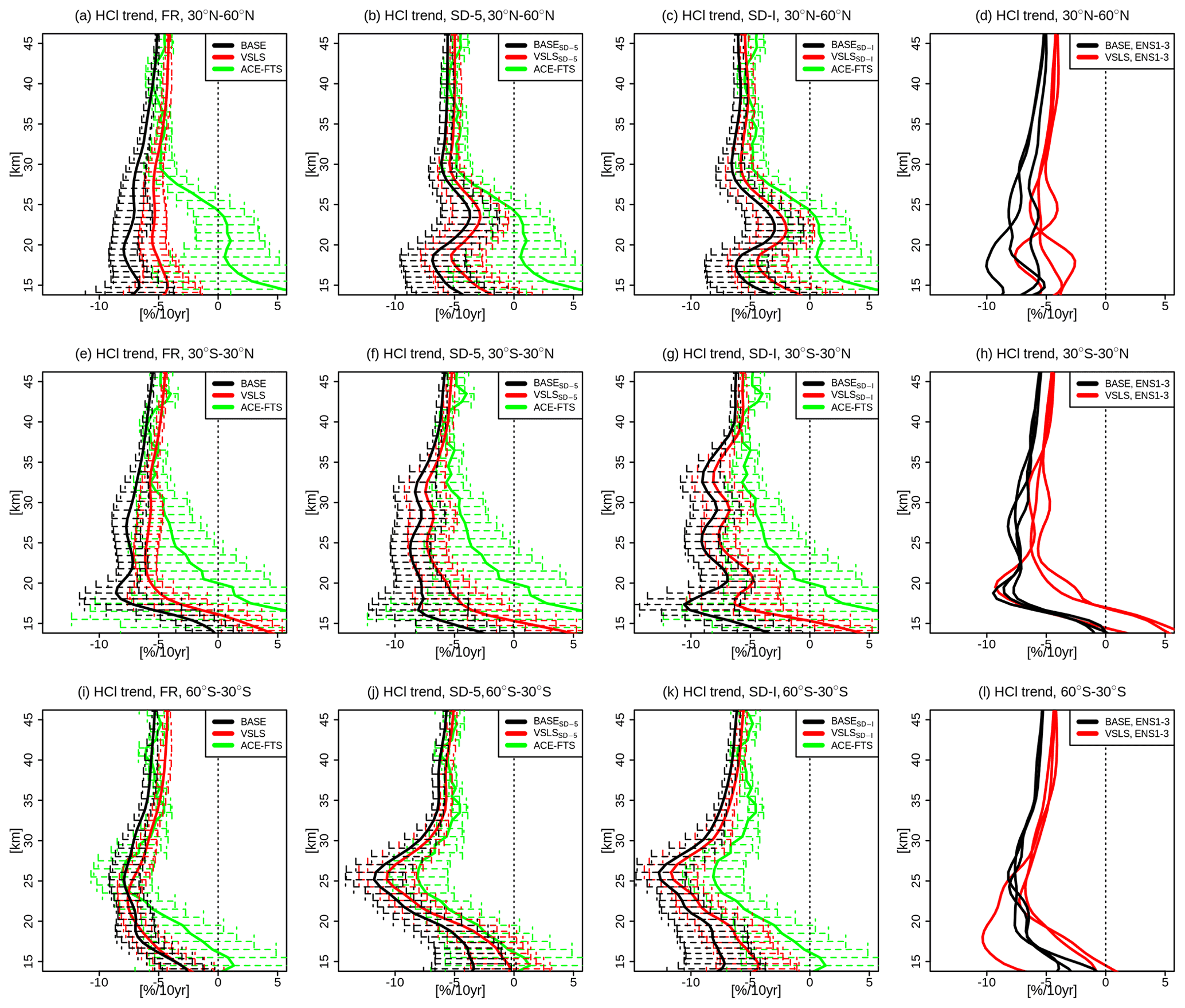
Figure 9 Linear trends in deseasonalised HCl mixing ratios [% per 10 years] averaged over (top) 30–60^∘ N, (middle) 30^∘ S–30^∘ N and (bottom) 30–60^∘ S. Left to right panels in each row are for: (a, e, i) the ensemble mean VSLS (red), ensemble mean BASE (black) and ACE-FTS (green); (b, f, j) VSLS_SD-5 (red), BASE_SD-5 (black) and ACE-FTS (green); (c, g, k) VSLS_SD-I (red), BASE_SD-I (black) and ACE-FTS (green); (d, h, l) the individual VSLS ensemble members (red) and the individual BASE ensemble members (black). Error bars indicate confidence intervals (±2 standard errors); error bars are not plotted in (d, h, l) for clarity.

We find that the inclusion of Cl-VSLS (Figs. 8a, 9) decreases the magnitude of the negative stratospheric HCl trend by around 25 % in the tropical lower stratosphere, i.e. from approximately −8 %/decade to −6 %/decade averaged over 30^∘ S–30^∘ N at 20 km in BASE and VSLS, respectively (Fig. 9e), The HCl trend derived from the VSLS run in the tropics agrees better with the ACE-FTS data in the lower and mid-stratosphere than the HCl trend diagnosed from BASE. In the tropical upper troposphere, the inclusion of Cl-VSLS significantly magnifies the positive HCl trend, which, in the VSLS run, reaches up to approximately 14 %/decade at 10 km compared to 4 %/decade in BASE.

Figure 10 As in Fig. 8a–f but for trends in deseasonalised model AoA [day per 10 years].

Notably, the observed ACE-FTS HCl trend displays a strong hemispheric asymmetry in the lower/mid-stratosphere, with a statistically significant negative trend (up to approximately −10 %/decade) in the Southern Hemisphere (SH) mid-latitudes, and a very weak, non-significant trend in the NH mid-latitudes (Fig. 8g). This asymmetry has been shown to arise due to the corresponding dynamical variability characterising the recent period (e.g. Mahieu et al., 2014), in particular, the apparent southward shift of the BDC found in the observational data (e.g. Ploeger et al., 2015; Wargan et al., 2018). Such horizontal pattern in the lower stratospheric HCl trend is not reproduced by either the ensemble mean VSLS or BASE runs. This is because the use of an ensemble mean of free-running integrations effectively minimises the effects of any short-term dynamical variability as illustrated by only very small trends in the corresponding ensemble mean AoA in these runs (Fig. 10a, b).

4.2 Free-running vs. nudged simulations

In contrast to the free-running integrations, the two pairs of nudged simulations (VSLS_SD-5/BASE_SD-5 and VSLS_SD-I/BASE_SD-I), by construction, show similar interannual dynamical variability to observations. In particular, all display a negative AoA trend (i.e. younger air) in the SH mid-latitudes and a positive trend (i.e. older air) in the NH mid-latitudes (Fig. 10c–f). This is a consequence of the apparent southward shift of the BDC reported from observational data. Since younger air is associated with lower concentrations of HCl (and vice versa for older air), the HCl trends diagnosed from the nudged runs show strong hemispheric asymmetry (Fig. 8c–f), with markedly stronger (i.e. more negative) HCl trend in the SH mid-latitudes and a weaker (i.e. less negative) HCl trend in the NH mid-latitudes. Such pattern is thus more similar to that found from the ACE-FTS data. While the agreement in the diagnosed HCl trends between the runs nudged to ERA5 and ERA-Interim reanalysis is much closer than between the nudged and free-running integrations, there are still some important qualitative differences between the nudged runs. This is particularly true in the SH lower stratosphere in accord with differences in the associated AoA trends in that region.

As was the case with the free-running integrations, the inclusion of Cl-VSLS improves the agreement between the simulated and ACE-FTS HCl trends in the tropical lower and mid-stratosphere (Fig. 9b). It also improves the agreement in the NH and SH mid-latitudes (Fig. 9a, c), which was not necessarily the case in the free-running integrations due to the role of short-term dynamical variability described above.

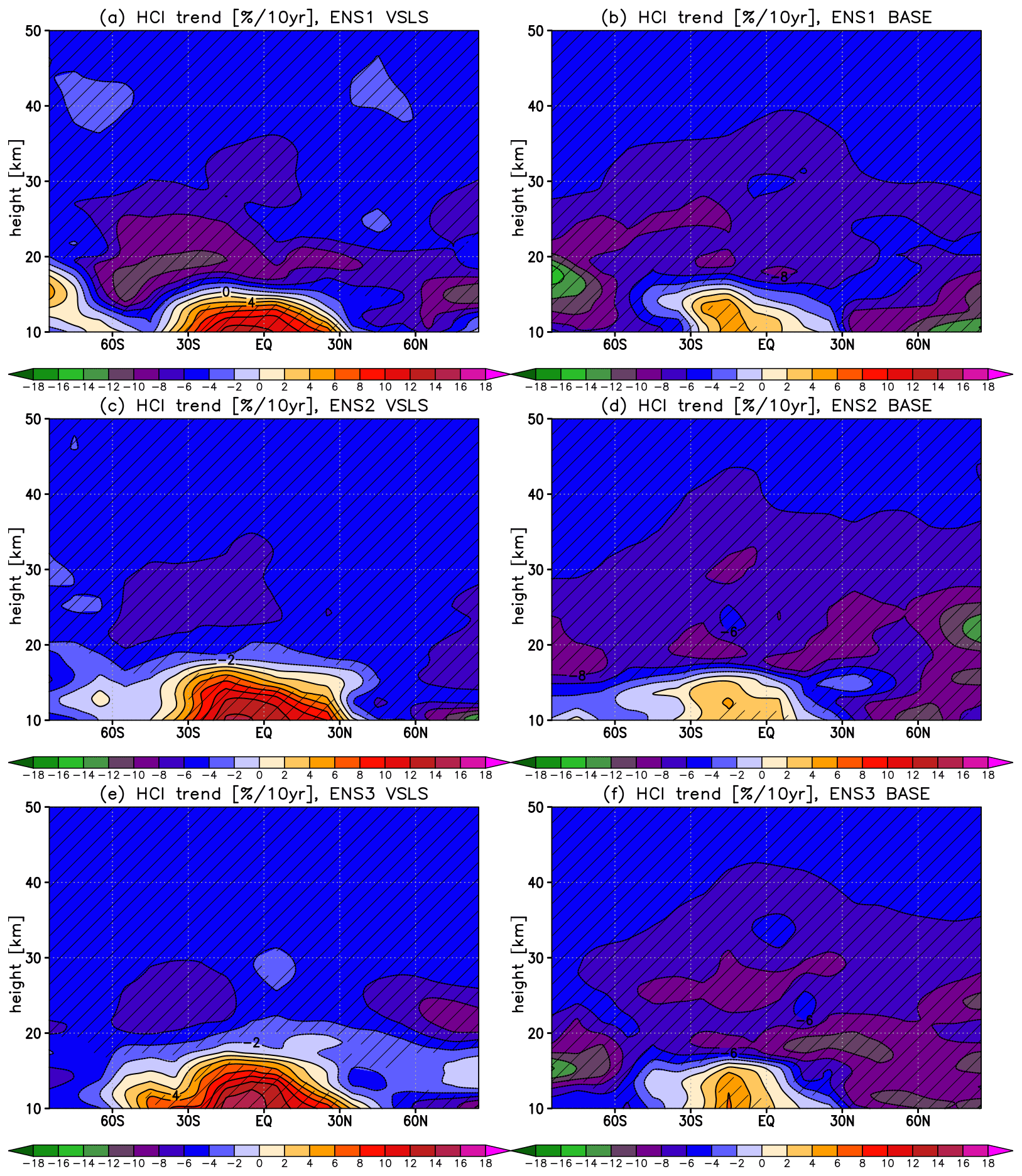
Figure 11 Linear MAM2004-SON2019 trends in deseasonalised HCl mixing ratios [% per 10 years] derived from the individual VSLS ensemble members: (a) ENS1 VSLS, (c) ENS2 VSLS and (e) ENS3 VSLS, and from the individual BASE ensemble members: (b) ENS1 BASE, (d) ENS2 BASE and (f) ENS3 BASE. Hatching indicates statistical significance (as in Fig. 6).

4.3 Individual ensemble members

Lastly, despite the same boundary conditions and forcings, we diagnosed a considerable range of HCl trends and their horizontal structures from the individual ensemble members of the free-running integrations (Fig. 9d, h, l for the trends in the NH mid-latitudes, tropics and SH mid-latitudes, respectively; Fig. 11). For example, the HCl trends in the SH mid-latitudes from the individual VSLS ensemble members at ∼17 km vary by over a factor of 3 from $\sim -\mathrm{10}$ %/decade in ENS1 to $\sim -\mathrm{3}$ %/decade in ENS3 (Fig. 9l). This illustrates the role of natural interannual variability in atmospheric circulation in modulating the HCl concentrations and, hence, the diagnosed HCl trends. A range of trends in model AoA are found over this ∼15-year period from the individual ensemble members of both VSLS and BASE experiments, with the different members displaying opposing positive and negative AoA trends that appear statistically significant (Fig. S5). This reaffirms the need for caution when interpreting both model and observationally derived trends in atmospheric tracers when calculated over such relatively short time periods.

5 The impacts of Cl-VSLS on COCl₂ trends

This section discusses recent rends in phosgene, an important product of Cl-VSLS oxidation and an atmospheric degradation product of the longer-lived CCl₄ and CH₃CCl₃ (e.g. Fu et al., 2007; Harrison et al., 2019).

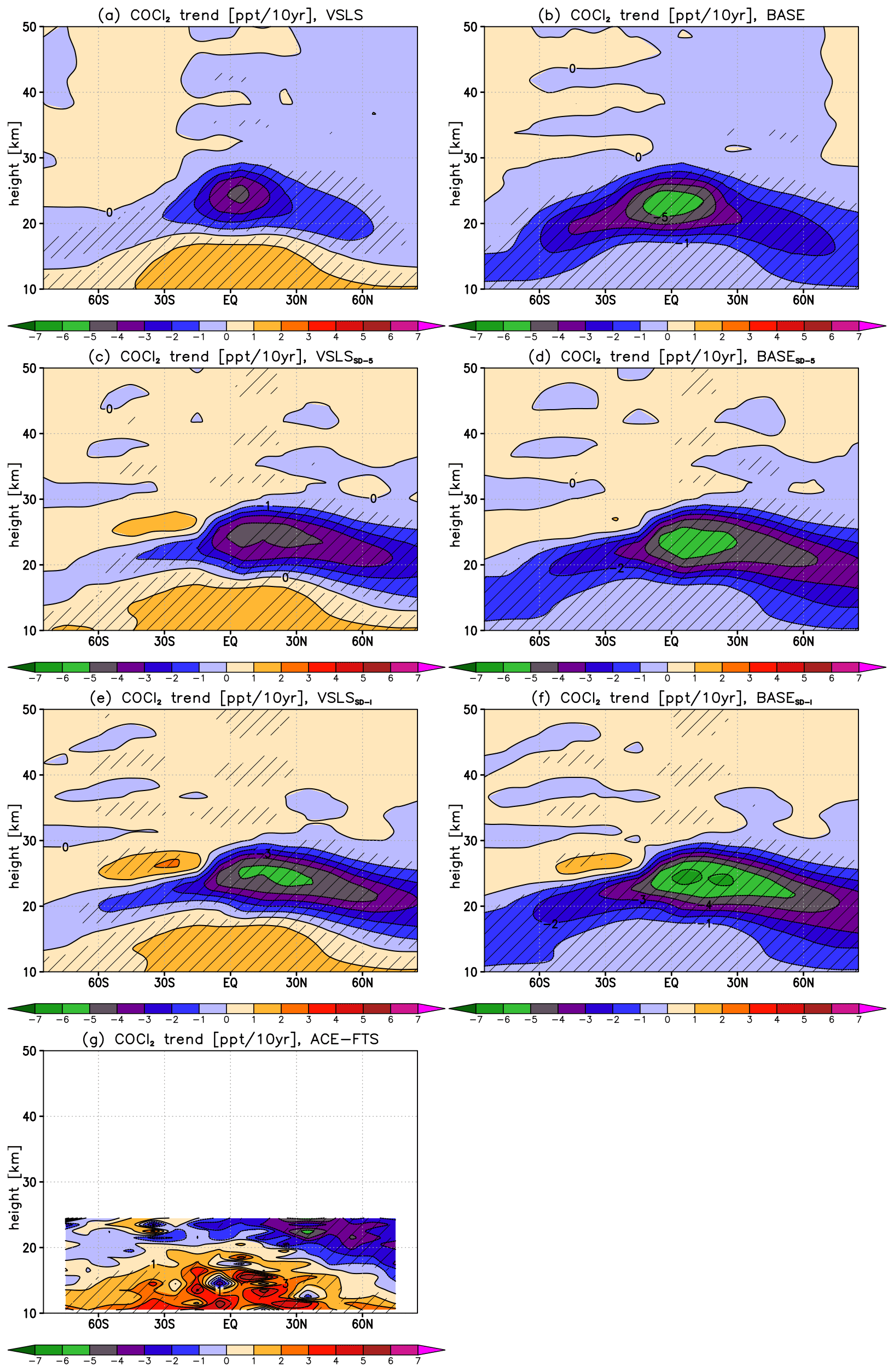
Figure 12 As in Fig. 8 but for linear trends in deseasonalised COCl₂ mixing ratios [ppt per 10 years].

5.1 Ensemble mean free-running simulations

Figure 12 shows linear trends in deseasonalised COCl₂ mixing ratios over 2004–2019 analogous to the HCl trends in Fig. 8. Consistent with concurrent long-term decline in atmospheric concentrations of CCl₄ and CH₃CCl₃ (WMO, 2018) and total inorganic chlorine, the stratospheric COCl₂ levels have decreased over the recent past, as illustrated by the negative COCl₂ trend in the ensemble mean BASE diagnosed throughout the lower stratosphere (Fig. 12b). We find that the inclusion of Cl-VSLS significantly decreases the magnitude of this negative stratospheric COCl₂ trend, with its maximum amplitude of $\sim -\mathrm{5}$ and $\sim -\mathrm{4}$ ppt/decade for the ensemble mean BASE and VSLS, respectively (Fig. 12a–b). Averaged over the tropics, this corresponds to a weakening of the trend from $\sim -\mathrm{4}$ to $\sim -\mathrm{2}$ ppt/decade at 21 km for BASE and VSLS, respectively (Fig. S7e). In the troposphere, while only very small and negative trend was simulated in the ensemble mean BASE, the inclusion of Cl-VSLS leads to a small but positive, statistically significant COCl₂ trend (∼1 ppt/decade at 10 km in the tropics). A qualitatively similar positive tropospheric COCl₂ trend was also found from the observed ACE-FTS data (Fig. 12g). Averaged over the tropics (30^∘ S–30^∘ N), the COCl₂ trend derived from VSLS thus agrees better with the ACE-FTS data throughout the troposphere and lower stratosphere than the COCl₂ trend diagnosed from BASE (Fig. S7).

5.2 Free-running vs. nudged simulations

While the COCl₂ trends diagnosed from the ensemble mean of free-running integrations are symmetrical in both hemispheres, this is not the case in the nudged runs (Fig. 12c–f). In particular, the COCl₂ trends diagnosed from the nudged runs are stronger (i.e. more negative) in the NH tropics and mid-latitudes than it is the case in the free-running integrations; the maximum amplitudes of the trends are also larger. In the SH sub-tropical and mid-latitudes, the COCl₂ trends at ∼25 km are small but positive. Such horizontal structure is qualitatively similar to that found in the observed ACE-FTS data (Fig. 12g), and is related to the southward shift of the upwelling part of the BDC (Sect. 4.2) which increases COCl₂ in the SH sub-tropics and decreases it in the NH.

As was the case with the free-running integrations, the inclusion of Cl-VSLS improves the agreement between the model and ACE-FTS COCl₂ trends in the tropics (Fig. S7). The agreement also improves in the NH and SH mid-latitudes (Fig. S7), which was not necessarily the case in the free-running integrations due to the influence of short-term dynamical variability described above. Regarding the role of the choice of reanalysis used for nudging, we find that the COCl₂ trends in the two sets of nudged runs are overall similar, albeit with somewhat stronger amplitudes of both the positive and negative responses simulated in the runs nudged to the ERA-Interim reanalysis (VSLS_SD-I and BASE_SD-I).

5.3 Individual ensemble members

Unlike for HCl, the COCl₂ trends derived from the individual ensemble members of the free-running integrations are largely in agreement with each other. There is still some variability in the magnitudes of the diagnosed trends, in particular in the mid-/high latitudes (see Figs. S6 and S7) due to the role of natural interannual variability.

6 Summary

Impacts of chlorinated very short-lived substances on stratospheric chlorine budget over the recent past (up to and including the year 2019) were assessed using the UM-UKCA chemistry–climate model. Our study constitutes the most up-to-date assessment of the impacts of Cl-VSLS. It is also the first published study to examine this topic not only using a CCM but also a whole atmosphere model, thereby simulating surface Cl-VSLS emissions, their tropospheric chemistry and transport, and the resulting stratospheric impacts in a fully consistent manner.

First, we quantified the transport of Cl-VSLS into the stratosphere using a small ensemble of free-running simulations. We estimated that the stratospheric source gas injection of chlorine from Cl-VSLS doubled over the first two decades of the 21st century at ∼80 ppt Cl in 2019 compared to ∼40 ppt Cl in 2000. Combined with the additional chlorine reaching the stratosphere in the form of product gases, we found that Cl-VSLS provided ∼130 ppt Cl to the stratosphere in 2019 (compared to ∼70 ppt in 2000). The average 2010–2019 difference of ∼100 ppt additional chlorine in the lower/mid-stratosphere in the experiment with Cl-VSLS accounted for ∼3 % of total stratospheric chlorine for that period. Thereby, it constituted a small but nonetheless important and growing contribution to the overall chlorine budget that is moreover changing in the opposite sense (i.e. increases in time) to the contribution from the long-lived ODSs.

The choice between a free-running versus nudged model set-up in UM-UKCA was found to have important consequences for the diagnosed atmospheric Cl-VSLS response. First, the use of the nudged set-up significantly increased the abundance of Cl-VSLS in the lower stratosphere relative to the analogous free-running UM-UKCA simulations. Averaged over 2010–2018, the simulation nudged to the ERAI-Interim reanalysis showed 20 ppt more Cl (i.e. a factor of 2) in the tropical lower stratosphere (25^∘ S–25^∘ N, 20 km) in the form of Cl-VSLS source gases compared to the free-running case. This arose because of a markedly faster large-scale atmospheric circulation simulated in the nudged run. In comparison, the run nudged to ERA5 showed 10 ppt more Cl (i.e. ∼50 %) in this region in the form of Cl-VSLS source gases than the free-running case, commensurate with smaller differences in the diagnosed transport between the two. Secondly, despite larger abundance of Cl-VSLS source gases simulated in the lower stratosphere in the nudged runs than in the free-running ones, the corresponding changes in total stratospheric chlorine were slightly smaller. This also related to the faster circulation in the nudged runs and indicated reduced concentrations of product gases (e.g. HCl), as opposed to source gases, and faster removal of inorganic chlorine from the stratosphere. Regarding the model transport itself, we found that the age-or-air in the UM-UKCA simulations nudged to the ERA-Interim reanalysis compared better with that derived from the MIPAS satellite data in the tropics than for the other simulations; however, this was not the case in the mid- and high latitudes.

Our results highlight the importance of model dynamical fields on transport of Cl-VSLS into the lower stratosphere. In UM-UKCA, this corresponds to the strong dependence of the diagnosed stratospheric Cl-VSLS levels on the choice between the free-running and nudged model set-up, and also on the choice of reanalysis dataset used for nudging. Given that the impact of nudging on the large-scale residual circulation does not necessarily improve its representation in CCMs (Orbe et al., 2018; Chrysanthou et al., 2019), our results illustrate explicitly the first-order impact this can have on simulated atmospheric tracers and their responses to external perturbations.

We also investigated the impact of the growth in the atmospheric Cl-VSLS concentrations on the early 21st century HCl and COCl₂ trends. We found that the inclusion of Cl-VSLS significantly reduced the magnitudes of the negative HCl and COCl₂ trends in the stratosphere (e.g. from $\sim -\mathrm{8}$ %(HCl)/decade and $\sim -\mathrm{4}$ ppt(COCl₂)/decade in the tropics at ∼20 km to $\sim -\mathrm{6}$ %(HCl)/decade and ∼ −2 ppt(COCl₂)/decade in the free-running simulations), and led to positive trends in these tracers in the troposphere. In the tropics, both free-running and nudged integrations with Cl-VSLS included compared better to the observed trends than analogous simulations without Cl-VSLS. Unlike the nudged runs, the ensemble mean free-running integrations did not reproduce the hemispheric asymmetry in the observed mid-latitude HCl and COCl₂ trends related to short-term dynamical variability over the recent period. Thus, while accurately reflecting an average Cl-VSLS response under “mean” dynamical conditions, the ensemble mean free-running integrations may be less useful for direct comparison with atmospheric observations (since the real world effectively constitutes only one ensemble member). Indeed, a comparison of HCl trends derived from the individual ensemble members of the free-running integrations revealed a considerable spread of the diagnosed tracer trends, illustrating the role of natural interannual variability in modulating the diagnosed responses. Our results highlight the need for caution when interpreting both model and observed tracer trends derived over a relatively short time period (here ∼15 years).

The results in this paper constitute Part 1 of a three-part study of atmospheric impacts of Cl-VSLS. In the follow up to this work, we will focus on the impacts of Cl-VSLS on stratospheric ozone (Part 2), and compare simulations forced with lower boundary conditions of Cl-VSLS, as used here, with simulations using recently estimated Cl-VSLS emissions from Claxton et al. (2020) (Part 3).