Investigating the global OH radical distribution using steady-state approximations and satellite data

We present a novel approach to derive indirect global information on the hydroxyl radical (OH), one of the most important atmospheric oxidants, using state-of-the-art satellite trace gas observations (key sinks and sources of OH) and a steady-state approximation (SSA). This is a timely study as OH observations are predominantly from spatially sparse field and infrequent aircraft campaigns, so there is a requirement for further approaches to infer spatial and temporal information on OH and its interactions with important climate (e.g. methane, CH₄) and air quality (e.g. nitrogen dioxide, NO₂) trace gases. Due to the short lifetime of OH (∼1 s), SSAs of varying complexities can be used to model its concentration and offer a tool to examine the OH budget in different regions of the atmosphere. Here, we use the well-evaluated TOMCAT three-dimensional chemistry transport model to identify atmospheric regions where different complexities of the SSAs are representative of OH. In the case of a simplified SSA (S-SSA), where we have observations of ozone (O₃), carbon monoxide (CO), CH₄ and water vapour (H₂O) from the Infrared Atmospheric Sounding Interferometer (IASI) on board ESA's MetOp-A satellite, it is most representative of OH between 600 and 700 hPa (though suitable between 400–800 hPa) within ∼20 %–30 % of TOMCAT modelled OH. The same S-SSA is applied to aircraft measurements from the Atmospheric Tomography Mission (ATom) and compares well with the observed OH concentrations within ∼26 %, yielding a correlation of 0.78. We apply the S-SSA to IASI data spanning 2008–2017 to explore the global long-term inter-annual variability of OH. Relative to the 10-year mean, we find that global annual mean OH anomalies ranged from −3.1 % to +4.7 %, with the largest spread in the tropics between −6.9 % and +7.7 %. Investigation of the individual terms in the S-SSA over this time period suggests that O₃ and CO were the key drivers of variability in the production and loss of OH. For example, large enhancement in the OH sink during the positive 2015/2016 El Niño–Southern Oscillation (ENSO) event was due to large-scale CO emissions from drought-induced wildfires in South East Asia. The methodology described here could be further developed as a constraint on the tropospheric OH distribution as additional satellite data become available in the future.

1 Introduction

The hydroxyl radical (OH) is a key species in atmospheric chemistry as it largely determines the oxidation capacity of the troposphere, and therefore the lifetimes of many different species. Key species controlled by OH include important greenhouse gases (e.g. methane, CH₄), ozone-depleting substances (e.g. hydrochlorofluorocarbons), and other short-lived anthropogenic and natural pollutants (e.g. volatile organic compounds (VOCs), nitrogen oxides (NO_x) and carbon monoxide (CO); Lelieveld et al., 2016). The importance of OH to tropospheric oxidation capacity was recognised in the early 1970s (Levy, 1971) and has been subject to many scientific investigations since, especially in relation to the lifetime of CH₄ (e.g. McNorton et al., 2016; Rigby et al., 2017; Turner et al., 2019). A better understanding of the spatial and temporal distribution of OH, the primary sink of CH₄, would aid the interpretation of recent trends in CH₄, such as the 2000–2007 concentration stabilisation period (Turner et al., 2019).

The primary source of OH in the remote troposphere is the photolysis of ozone (O₃) by ultraviolet (UV) radiation (<330 nm wavelength). This forms O(¹D), which then reacts with water vapour (H₂O) to form OH (Lelieveld et al., 2016).

$$\begin{array}{}\text{(1)}& {\displaystyle }{\mathrm{O}}_{\mathrm{3}}+\mathrm{hv}\left(\mathit{\lambda }<\mathrm{330}\mathrm{nm}\right)\to \mathrm{O}\left({}^{\mathrm{1}}\mathrm{D}\right)+{\mathrm{O}}_{\mathrm{2}}\text{(2)}& {\displaystyle }\mathrm{O}\left({}^{\mathrm{1}}\mathrm{D}\right)+{\mathrm{H}}_{\mathrm{2}}\mathrm{O}\to \mathrm{2}\mathrm{OH}\end{array}$$

The OH radical formed is very reactive due to the unpaired electron on the oxygen atom. After formation, the OH radicals attack reduced and partly oxidised gases, removing them from the atmosphere and forming peroxy radicals (e.g. hydroperoxyl radical, HO₂). The peroxy radicals can go on to form peroxides and participate in many other atmospheric chemistry reactions (e.g. ozone formation) and can also go on to reform OH (Lelieveld et al., 2016).

Direct in situ measurements of OH are scarce as the measurement process is challenging, with few instruments available (Stone et al., 2012; Lelieveld et al., 2016). Due to its very short lifetime, ∼1 s in the daytime, the abundance of OH is very low, with the global tropospheric mean OH concentration around 1×10⁶ molec. cm⁻³. In situ OH measurements are limited to field campaigns at specific locations (Stone et al., 2012) and aircraft missions, e.g. NASA's Atmospheric Tomography mission (ATom; Wofsy et al., 2018; Brune et al., 2020). There has consequently been a demand for indirect methods to infer global-scale OH. An established method is to use the methyl chloroform (CH₃CCl₃, MCF) concentrations to derive a global mean OH concentration by using inverse modelling, which exploits the fact that sources of MCF are well known and that its main sink is reaction with OH (Lovelock, 1977; Singh, 1977; Prinn et al., 1992). This method has been used to study the temporal variability of OH (Montzka et al., 2011; Prinn et al., 2005). The accuracy of this method depends on accurate estimates of MCF emissions. MCF production is regulated under the legislation initiated by the 1987 Montreal Protocol, and therefore MCF has seen a sharp decline in atmospheric abundance since the mid-1990s, which will reduce the viability of this method, leading to new methods and tracers being sought (Huang and Prinn, 2002; Liang et al., 2017; Rigby et al., 2017).

However, the above-mentioned MCF method is unable to provide spatial information on OH. In the last 2 decades, there has been an increasing wealth of tropospheric satellite data, providing information on the spatial and temporal variability of atmospheric species, but not OH (Streets et al., 2013). These atmospheric composition data are global in extent and now span more than a decade, so they have the potential to provide information to infer a global OH distribution and its variation over time. Presently, there are limited examples of the use of satellite data to infer global OH. In a recent study, Wolfe et al. (2019) used satellite formaldehyde observations and budget to calculate remote tropospheric column OH, developing the method using aircraft data from ATom to establish formaldehyde production/loss and OH concentrations.

To exploit satellite data here, we use a simplified steady-state approximation. This is an appropriate assumption due to the very short daytime lifetime of OH, and the simplification is described in Sect. 2 below. Some studies have thus far used steady-state approximations to calculate OH from in situ surface data at field sites, e.g. Eisele (1996) at Mauna Loa Observatory; Savage et al. (2001) and Smith et al. (2006) at the Mace Head Atmospheric Research Centre, Ireland; Creasey et al. (2003) at Cape Grim in the Southern Ocean; and Slater et al. (2020) in central Beijing. However, there is also the potential for these approximations to be applied to satellite data in a global context. The use of the steady-state approximations has had varied success. Eisele (1996) found that the comparison between observed and calculated OH depended on which air mass was present, with free tropospheric air masses showing better agreement than air masses from the boundary layer. Savage et al. (2001) found a good correlation between measured and calculated OH, but a steady-state overprediction of around 30 %. Models using only simplified chemistry have been shown to capture the chemistry of unpolluted regions. Sommariva et al. (2004) used a “detailed” and “simple” box model to study OH in unpolluted marine air at Cape Grim in the Southern Hemisphere (SH). The simple box model, based only on CO, CH₄ and inorganic reactions, agreed within 5 %–10 % of the detailed box model that also contained non-methane hydrocarbons (NMHCs). The models over-estimated the measured OH by 10 %–20 %.

OH reactivity (OHR), the inverse of OH lifetime, is also measured in the field to provide additional information on the tropospheric oxidation capacity and abundance of the OH radical. OHR can be measured in situ along with trace gas concentrations, e.g. during aircraft campaigns such as NASA's ATom (Wofsy et al., 2018). Observed OHR is commonly compared to calculated OHR by summing individual sink terms using measured reactant concentrations multiplied by their respective reaction rate coefficients with OH (Yang et al., 2016). However, a large number of field campaigns have shown that there is often a substantial difference between observed in situ and calculated OHR, known as the “missing” reactivity (Ferracci et al., 2018). This missing reactivity can account for as much as 20 % (usually outside the OHR uncertainty range) to 80 % of the observed OHR (Yang et al., 2016). There are many proposed reasons for this missing reactivity, such as short-lived VOCs that were not measured (Kovacs et al., 2003) or in the rainforests some mixture of unidentified biogenic emissions and photo-oxidation products (Edwards et al., 2013; Nölscher et al., 2016).

An improved characterisation of the OH temporal variation is vital to understanding key aspects of atmospheric chemistry, such as interannual to decadal variability in methane (Turner et al., 2019; Zhao et al., 2020). Studies using MCF observations, in combination with box-model analyses, show similar annual OH anomalies between 1995 and 2010, with a broadly negative anomaly of −6 % to 0 % between 1995 and 1999, a positive anomaly of 0 % to 6 % between 1999 and 2007, and a negative anomaly of −5 % to 0 % between 2007 and 2010 (Montzka et al., 2011; Rigby et al., 2017; Turner et al., 2017; Patra et al., 2021). After 2010, the results of such studies differ, with some showing consistently negative anomalies of −4 % to 0 % between 2010 and 2018 (Rigby et al., 2017; Turner et al., 2017) and others showing some positive anomalies in this period, for example in the range of 0 % to 4 % between 2010 and 2015 (Naus et al., 2019; Patra et al., 2021). Studies using chemical transport models are not consistent with those using MCF observations. He et al. (2020) found negative anomalies of −5 % to 0 % between 1995 and 2005 and then positive anomalies of 0 % to 4 % between 2005 and 2017. A study by Zhao et al. (2020) found a multi-model mean increase of 0.7×10⁵ molec. cm⁻³ between 1980 and 2010, equivalent to around 0.1 %–0.5 % yr⁻¹, with the greatest rate of increase in the final decade (2000–2010). The OH increase from 2000–2010 was predominantly due to that in the primary production term (O(¹D) + H₂O) though also to a decrease in the CO sink term (OH + CO). Model studies further show OH interannual variability to be influenced by the El Niño–Southern Oscillation (ENSO), with low OH concentrations being associated with El Niño years and high OH concentrations with La Niña years (Zhao et al., 2020; Anderson et al., 2021).

Here, we use output data from the TOMCAT 3D chemical transport model to explore the validity of OH steady-state approximations in the troposphere. A simplified steady-state approximation is then applied to observations of O₃, CO, CH₄ and H₂O mid-tropospheric concentrations retrieved from observations by the Infrared Atmospheric Sounding Interferometer (IASI) instrument on board the MetOp-A satellite in 2010 and 2017. This calculated satellite OH is then compared to OH from TOMCAT using full chemistry and ATom observations. Finally, the simplified approximation is applied to MetOp-A data over a 10-year period (2008–2017) to infer the temporal variability in OH. Section 2 describes how steady-state approximations, TOMCAT model, aircraft and satellite data are employed in this study. Section 3 presents the results and discussion. Section 4 summarises our conclusions.

2 Methods

2.1 OH steady-state approximations

Due to the short lifetime of OH, a steady-state approximation can be used to model its concentration. The approximation can be defined as Eq. (3):

$$\begin{array}{}\text{(3)}& [\mathrm{OH}{]}_{\mathrm{Steady}\mathrm{State}}={\displaystyle \frac{k_{A+B}\left[A\right]\left[B\right]+\mathrm{\dots }+j_C\left[C\right]+\mathrm{\dots }}{\sum k_D\left[D\right]+\mathrm{\dots }}},\end{array}$$

where the numerator of the expression represents a sum of the source terms. k_A+B is the reaction rate constant of A and B to form OH, and j_C is the photolysis coefficient of C to form OH. The denominator represents a sum of the sink terms. k_D is the reaction rate constant of D and OH, where D represents an individual sink species. The accuracy of the approximation depends partly on the number of source and sink terms which can be included. This, in turn, depends on the availability of observations to provide a constraint for each of those terms.

Here, we use three steady-state approximations of different complexity, summarised in Table S1 in the Supplement. The most complex is referred to as the full-chemistry steady-state approximation (FC-SSA) and contains the largest number of source and sink terms, capturing the most comprehensive tropospheric chemistry, with 26 source terms and 51 sink terms. The second most complex is based on a steady-state approximation in Savage et al. (2001; Sav-SSA) and contains five source and 12 sink terms. Lastly, we propose a simplified steady-state approximation (S-SSA) containing one source term (based on Eqs. 1 and 2) and three sink terms (based on the reaction of OH with CH₄, CO and O₃). The S-SSA allows OH to be derived using only the main tropospheric source and sinks that can be directly observed by satellite. We adopt the S-SSA as Eq. (4):

$$\begin{array}{}\text{(4)}& {\left[\mathrm{OH}\right]}_{\mathrm{Steady}\mathrm{State}}={\displaystyle \frac{\left(\frac{\mathrm{2}{j}_{\mathrm{1}}{k}_{\mathrm{1}}\left[{\mathrm{O}}_{\mathrm{3}}\right]\left[{\mathrm{H}}_{\mathrm{2}}\mathrm{O}\right]}{k_{\mathrm{2}}\left[{\mathrm{N}}_{\mathrm{2}}\right]+k_{\mathrm{3}}\left[{\mathrm{O}}_{\mathrm{2}}\right]+k_{\mathrm{1}}\left[{\mathrm{H}}_{\mathrm{2}}\mathrm{O}\right]}\right)}{\left(k_{\mathrm{4}}\left[{\mathrm{CH}}_{\mathrm{4}}\right]+k_{\mathrm{5}}\left[\mathrm{CO}\right]+k_{\mathrm{6}}\left[{\mathrm{O}}_{\mathrm{3}}\right]\right)}},\end{array}$$

where j₁ is the photolysis coefficient for O${}_{\mathrm{3}}\to \mathrm{O}\left({}^{\mathrm{1}}\mathrm{D}\right)+{\mathrm{O}}_{\mathrm{2}}$, k₁ is the reaction rate constant for O(¹D) + H₂O, k₂ and k₃ are the collisional relaxation rate constants with respect to N₂ and O₂, and k₄, k₅ and k₆ are the rate constants for reaction of OH with CH₄, CO and O₃, respectively. The expression implicitly assumes a steady state for the production and loss of O(¹D).

2.2 OH reactivity

OHR, the denominator of Eq. (3), can be directly observed or calculated using a model and/or observed species. The accuracy of an OHR calculation is similarly dependent on the number of sink terms that can be included and the availability of requisite observations. In principle, examination of OHR measurements co-located with those of [OH] could allow steady-state approximations for OH sources and sinks to be evaluated separately. We adopt the denominator of Eq. (4) as a simplified expression for OHR as Eq. (5):

$$\begin{array}{}\text{(5)}& \left[\mathrm{OHR}\right]=k_{\mathrm{4}}\left[{\mathrm{CH}}_{\mathrm{4}}\right]+k_{\mathrm{5}}\left[\mathrm{CO}\right]+k_{\mathrm{6}}\left[{\mathrm{O}}_{\mathrm{3}}\right].\end{array}$$

2.3 Model and observations

2.3.1 TOMCAT 3D model

In this study we use the 3D global chemical transport model TOMCAT (Chipperfield, 2006) at a $\mathrm{2.8}{}^{\circ }\times \mathrm{2.8}{}^{\circ }$ resolution with 31 vertical levels between the surface and 10 hPa. The model is coupled with the Global Model of Aerosol Processes (GLOMAP) to calculate aerosol microphysics (Mann et al., 2010). The model is forced by meteorological reanalyses (ERA-Interim) from the European Centre for Medium-Range Weather Forecasts (ECMWF; Dee et al., 2011). The tropospheric chemistry scheme is described in Monks et al. (2017), with the main updates as follows: anthropogenic and natural surface emissions from the Coupled Model Intercomparison Project Phase 6 (CMIP6) for NO_x, CO and VOCs (Feng et al., 2020); fixed annual biogenic emissions from the Chemistry-Climate Model Initiative (CCMI; Morgenstern et al., 2017); biomass burning emissions from the Global Fire Emissions Database (GFED) version 4 (van der Werf et al., 2017); CH₄ scaled to a best estimate based on the 2010 globally averaged surface CH₄ value from NOAA (Dlugokencky, 2020), and an update to the cloud fields using reanalyses from ECMWF (as described in Rowlinson et al., 2019). The model simulation was run for 2010 and 2017, with 6 months of spinup in each case. The simulation was sampled daily at 09:30 local solar time (LST) globally to match the MetOp-A daytime overpass time.

Monks et al. (2017) and Rowlinson et al. (2019) have evaluated TOMCAT OH compared to model and observational datasets for the year 2000. The set-up for the simulations used in Rowlinson et al. (2019) is most similar to that in this study, but broadly the simulation in Monks et al. (2017) produces similar regional zonal OH values. TOMCAT OH in Rowlinson et al. (2019) had an average global tropospheric concentration of 1.04×10⁶ molec. cm⁻³, which sits within a range from other studies, e.g. $\mathrm{0.94}\pm \mathrm{0.1}\times {\mathrm{10}}^{\mathrm{6}}$ molec. cm⁻³ from inferred OH observations from MCF by Prinn et al. (2001), $\mathrm{1.08}\pm \mathrm{0.6}\times {\mathrm{10}}^{\mathrm{6}}$ molec. cm⁻³ from the POLARCAT Model Intercomparison Project (POLMIP) and the multi-model mean of $\mathrm{1.11}\pm \mathrm{0.2}\times {\mathrm{10}}^{\mathrm{6}}$ molec. cm⁻³ from 16 Atmospheric Chemistry and Climate Model Intercomparison Project (ACCMIP) models (Naik et al., 2013). In terms of vertical distribution, Monks et al. (2017) and Rowlinson et al. (2019) show the maximum TOMCAT OH values to be between the surface and 750 hPa near the Equator. In comparison, Spivakovsky et al. (2000; MCF method) and the multi-model mean OH from ACCMIP (Naik et al., 2013) have peak OH values higher up in the troposphere. Overall, in the mid-troposphere, the primary focus in this study, Rowlinson et al. (2019) TOMCAT OH shows comparable values across all the latitude regions in comparison with Spivakovsky et al. (2000) and ACCMIP (Naik et al., 2013).

2.3.2 Satellite observations

We use satellite observations for 2010 and 2017 from the MetOp-A satellite launched by EUMETSAT in 2006. MetOp-A is in a polar sun-synchronous orbit which crosses the Equator at ∼09:30 LST (day overpass) and 21:30 LST (night overpass), giving global Earth coverage twice a day (Clerbaux et al., 2009). Here, we use height-resolved distributions of CO, CH₄, O₃ and H₂O retrieved from MetOp-A observations by schemes developed by the Rutherford Appleton Laboratory (RAL). The O₃, CO and H₂O retrievals are from the extended version of RAL's Infrared and Microwave Sounding (IMS-extended) scheme, which co-retrieves temperature profiles, cloud and surface properties, other trace gases, and aerosols and is documented in the supplement of Pope et al. (2021). The CH₄ data were produced by an improved version (v2.0) of RAL's methane retrieval scheme (Siddans et al., 2020) developed for IASI on MetOp-A. The original IASI methane scheme (v1.0) was described in Siddans et al. (2017). For the IMS-extended scheme, as well as the IASI methane scheme, retrieved profiles are output at the locations of IASI soundings. IASI is a nadir-viewing thermal infrared Fourier transform spectrometer, with a spectral range from 645 to 2760 cm⁻¹ (Clerbaux et al., 2009). It samples a swath width of 2200 km by scanning a set of four fields of view across-track. At nadir, these are circular with 12 km diameter, occupying a square 50 km × 50 km ($\mathrm{3.3}{}^{\circ }\times \mathrm{3.3}{}^{\circ }$). For the study of OH temporal variation between 2008 and 2017, MetOp-A data sub-sampled both temporally (1 in 10 d) and spatially (1 in 4 pixels) were available. Figures S1 and S2 in the Supplement show good agreement between the sub-sampled and fully sampled satellite data in a zonal average when compared in 2010 and 2017, with an average monthly correlation coefficient in latitudinal structure of 0.89 and 0.85, respectively.

Profiles of H₂O, O₃ and CO, along with temperature, are represented on a set of 101 levels in the IMS extended scheme. For H₂O, information from IASI and the two microwave sounders (Microwave Humidity Sounder (MHS) and Advanced Microwave Sounding Unit (AMSU-A)) is sufficient to resolve a number of independent layers between the surface and 200 hPa, with degrees of freedom of signal (DOFS) being typically ∼10. Profiles of H₂O (and temperature) produced from MetOp-A by the IMS core scheme have been validated against radiosondes in ESA's Climate Change Initiative (European Space Agency, unpublished) and found to have a systematic bias of ∼10 %. For CO, on the other hand, measurement information (exclusively from IASI) is sufficient to retrieve only one independent layer, with the averaging kernels centred on the mid-troposphere at ∼600 hPa with a full width half medium (FWHM) from ∼300–900 hPa, as seen in Figs. S3 and S4. Validation of the IMS-extended CO retrievals, through indirect comparisons using the Copernicus Atmospheric Monitoring Service (CAMS) in which averaging kernels were applied (see the supplement of Pope et al., 2021), found uncertainty in retrieved CO to be approximately 10 %. For O₃, averaging kernels peak at a number of levels spanning the troposphere and stratosphere, with DOFs generally ranging between 3.0 and 4.0. The lowest peak is seen in Figs. S3 and S4 to be around ∼600 hPa with FWHM from ∼350–900 hPa. When compared with ozonesondes (Sect. S3), O₃ retrieved in the mid-troposphere by the IMS-extended scheme is found to be systematically larger by up to 20 %. The RAL v2.0 IASI scheme retrieves CH₄ on a set of coarsely spaced levels, taking as input temperature profiles and surface spectral emissivity pre-retrieved from the same soundings by IMS. Output files also include layer-average mixing ratios and their corresponding averaging kernels, as shown in Figs. S3 and S4. The number of DOFS is greater than 2 in the tropics and drops to below 2 at polar latitudes; the surface–450 hPa layer average is well resolved from layers above. Examples of averaging kernels for H₂O, CH₄, CO and O₃ are shown in Sect. S2 (Figs. S3 and S4).

With the exception of H₂O, retrieval sensitivity is seen in Figs. S3 and S4 to decrease in the lowest atmosphere as temperature approaches that of the surface and surface–air temperature contrast on which sensitivity depends diminishes. However, in all four cases, averaging kernels for layers centred in the mid-troposphere are well behaved, with peaks around 600–700 hPa and FWHMs contained within the free troposphere, as appropriate for the focus of this study. For straightforward comparison with TOMCAT simulations, use of retrieved MetOp-A data is further restricted to the 400–800 and 600–700 hPa layers, where averaging kernels peak, rather than applying the averaging kernels to model profiles.

Co-located retrievals of H₂O, O₃ and CO data and CH₄ were filtered for a geometric cloud fraction of 20 % or less (i.e. 0.2 fractional coverage or less). This resulted in satellite soundings which exclude all opaque clouds which fill the field of view and a fraction of clouds which fill part of the field of view. In comparison with TOMCAT, which had no filtering for cloud, this could produce a clear skies bias. However, the model is driven by ECMWF meteorological fields, which are also used in the satellite retrieval, so they should be reasonably consistent. Figure S6 shows the daily average number of retrievals used per grid box for the calculation of satellite [OH]. Globally, the daily average number of grid-box profile retrievals for the input species ranges between 0 and 24, with an average of ∼6. Therefore, there are sufficient retrievals of the trace gases in the S-SSA to calculate values of OH for most grid boxes every day.

Uncertainty on [OH] calculated with the S-SSA using satellite data is estimated from the systematic errors on the four retrieved species, as described in Sect. S6, to be ∼23 %–24 % (Fig. S7). This assumes that there is no uncertainty in the rate constants (j₁, k₁₋₆), which is a potential source of error.

2.3.3 ATom observations

The ATom mission observed many atmospheric variables, including OH and OHR (Wofsy et al., 2018). NASA's DC-8 aircraft sampled the atmosphere between 0.2–12 km altitude during four campaigns between 2016–2018, sampling both hemispheres over the Pacific and Atlantic oceans. We use ATom observations of OH, OHR, O₃, CO, CH₄, H₂O and j₁. We use data from all four campaigns between and 08:00–11:00 LST, to compare with the 09:30 LST MetOp-A overpass time and the 600–700 hPa pressure range, where the S-SSA agrees best with the full chemistry (see Sect. 3.1). The data are also filtered to remove measurements influenced by stratospheric air (O${}_{\mathrm{3}}/$CO >1.25) or biomass burning (acetonitrile concentration >200 ppt), as in Travis et al. (2020). The OH and OHR observations used in this study were made by the ATHOS instrument (Faloona et al., 2004; Brune et al., 2020). Wofsy et al. (2018) merged the observations into a 2 min sampling interval. The uncertainty on the OH observations from the ATHOS instrument at the 2σ confidence level is ±35 % and the limit of detection of the OH observations is 0.018 pptv. The uncertainty on the OHR observations from the ATHOS instrument at the 2σ confidence level is ±0.8 s⁻¹. The NOAA Picarro instrument provides CH₄ and CO observations, with uncertainties of ±0.7 and ±8.9 ppbv, respectively (Karion et al., 2013). The diode laser hygrometer (DLH) provides H₂O observations with an uncertainty of ±5 % (Podolske et al., 2003). The NOAA-NO_y O₃ instrument provides O₃ observations with an average uncertainty of ±2.0 ppb (Ryerson et al., 2000). The CCD actinic flux spectroradiometer (CAFS) instrument provides j₁ observations, with an uncertainty of ±20 % (Shetter and Müller, 1999).

3 Results and discussion

3.1 Application of the simplified steady-state approximation

3.1.1 Application to model data

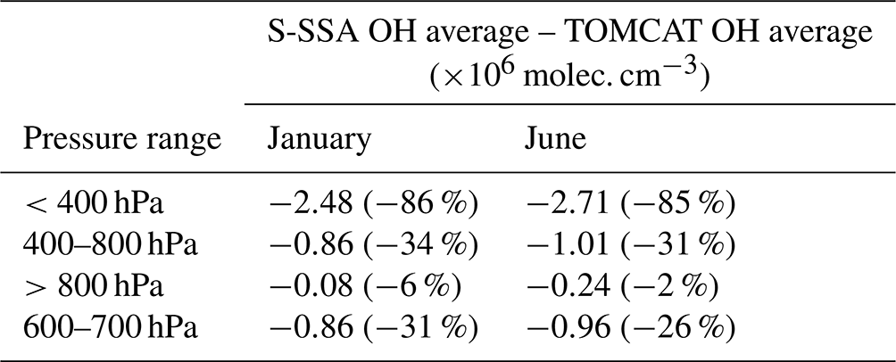
We use the TOMCAT output of CO, CH₄, O₃ and H₂O for 2010 in the S-SSA of OH to determine the validity of this approximation in different regions of the troposphere. Mass-weighted zonal mean [OH] calculated with the S-SSA and modelled TOMCAT [OH] are compared in Fig. 1. Table 1 shows the differences to be very large (>85 %) between global mean TOMCAT OH and TOMCAT S-SSA OH at pressures <400 hPa (i.e. upper troposphere and stratosphere). Nearer the surface (>800 hPa) the S-SSA shows a good zonal mean agreement (<6 % difference). However, there are large differences in the longitude–latitude distribution which do not show in the zonal mean, and we do not expect a good approximation of the complex OH chemistry in the boundary layer using our simplified approximation. Therefore, we focus our investigation at pressure levels above the boundary layer.

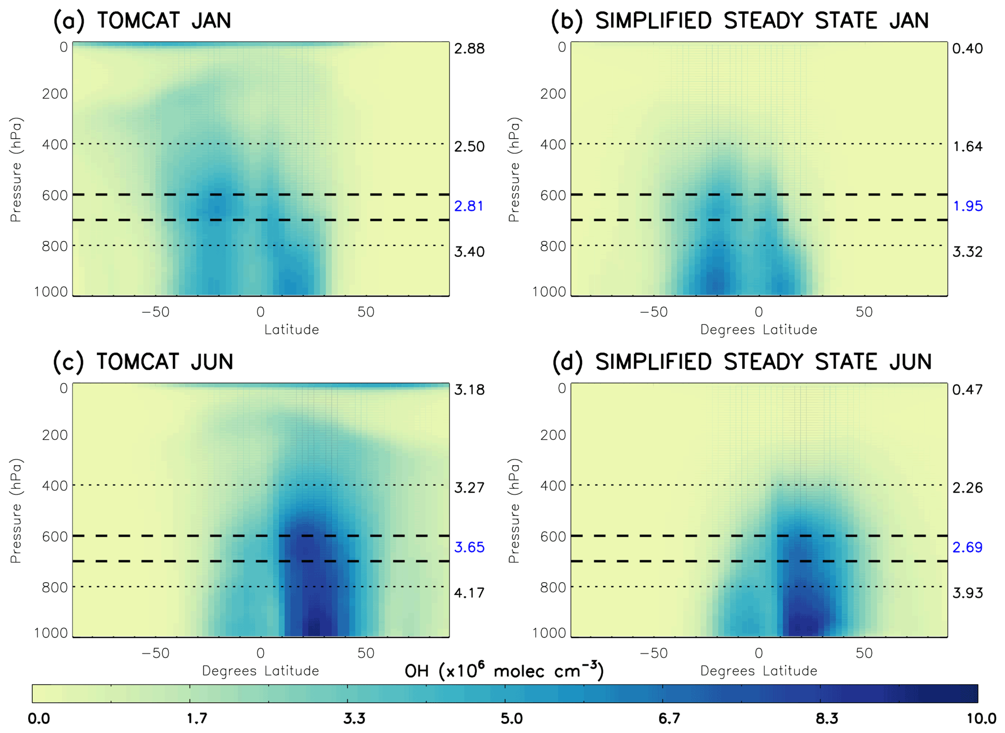
Figure 1 Comparison of TOMCAT OH and S-SSA OH in 2010: (a) TOMCAT OH January, (b) TOMCAT S-SSA OH January, (c) TOMCAT OH June and (d) TOMCAT S-SSA OH June. The dashed lines represent the proposed area of best agreement, 600–700 hPa. The numbers on the right of each plot represent the mass-weighted mean OH in ×10⁶ molec. cm⁻³ of the region shown by the dotted lines (from top to bottom): <400 hPa, between 400–800 hPa, and between 800 hPa and the surface.

Table 1 Comparison of mass-weighted global mean TOMCAT OH and S-SSA OH for different pressure ranges. Percentage difference relative to the TOMCAT OH mean given in brackets.

The mid-tropospheric region (400–800 hPa) shows good agreement in spatial distribution and abundance, with a S-SSA global mean underestimate of ∼30 %–35 %. In the mid-troposphere, there are peak values of 5.4×10⁶ molec. cm⁻³ (January) and 7.3×10⁶ molec. cm⁻³ (June) for TOMCAT S-SSA OH, which are comparable to peak values of 5.6×10⁶ molec. cm⁻³ (January) and 8.3×10⁶ molec. cm⁻³ (June) for TOMCAT OH. Within this mid-tropospheric region, the 600–700 hPa layer is further investigated, as it shows better agreement in the zonal mean structure and global mean than the larger pressure region, as shown in Table 1. TOMCAT output from 2017 was also applied to the S-SSA with similar results, shown in Sect. S7 (Fig. S9). We therefore selected the pressure region 600–700 hPa for investigation because of the good agreement between TOMCAT OH and TOMCAT S-SSA OH in this region. OH in this the pressure region contributes to ∼15 % of the tropospheric OH burden. Diagnosis of the model output shows the influence of OH on methane oxidation in this region is slightly larger, with a contribution of ∼19 % of methane-loss-weighted OH.

Figure 2 shows the spatial differences between the TOMCAT and S-SSA OH. In January, the S-SSA shows an underestimate of up to $\sim \mathrm{2}\times {\mathrm{10}}^{\mathrm{6}}$ molec. cm⁻³ across the Northern Hemisphere (NH) and over parts of the oceans across the SH, mostly between the Equator and 30^∘ S, e.g. the Atlantic and edges of the Pacific but not the Indian Ocean. In the SH, an overestimate is present over some of the continents, e.g. up to $\sim \mathrm{2}\times {\mathrm{10}}^{\mathrm{6}}$ molec. cm⁻³ in South America and up to $\sim \mathrm{1}\times {\mathrm{10}}^{\mathrm{6}}$ molec. cm⁻³ in the Indian Ocean and the centre of the Pacific. Broadly, the peak [OH] values across the SE Indian Ocean and southern African continent show good agreement. In June, the S-SSA shows good agreement over the oceans in the NH, mostly between the Equator and 30^∘ N, and the South American and Australian continents in the SH. An overestimate of up to $\sim \mathrm{4}\times {\mathrm{10}}^{\mathrm{6}}$ is found across the peak [OH] values found across the northern African continent and China. A slight underestimate of up to $\sim \mathrm{1}\times {\mathrm{10}}^{\mathrm{6}}$ is found on land masses around the Equator.

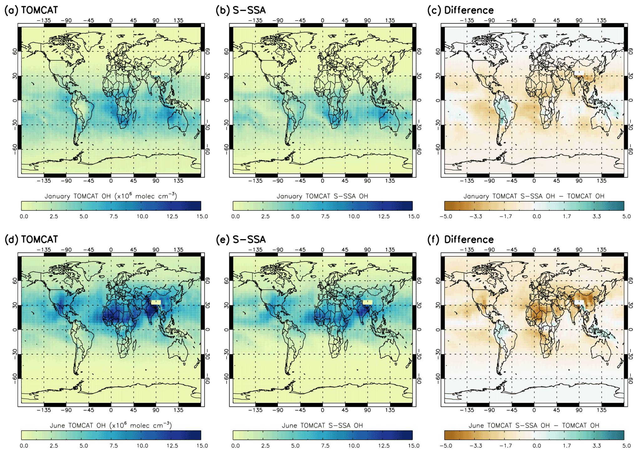
Figure 2 OH concentrations averaged over the 600–700 hPa range for TOMCAT, S-SSA and the difference (TOMCAT S-SSA minus TOMCAT). Panels (a)–(f) represent comparisons for January and June. All values are in in units of ×10⁶ molec. cm⁻³.

In summary, the S-SSA agrees with TOMCAT across the oceans near the Equator, to an extent which depends on the season. The peak values of [OH] are found in similar locations for TOMCAT and S-SSA [OH]; however, the S-SSA generally produces an underestimate of these peak values.

3.1.2 Study of reactions omitted from the S-SSA

The aim of this study is to derive information about OH from satellite data. Therefore, some source and sink reactions, which do not have relevant satellite retrievals, have been omitted from the S-SSA. We apply TOMCAT model data to another more complex steady-state approximation, Sav-SSA, to demonstrate which atmospheric species additional to H₂O, O₃, CO and CH₄ are key to OH production and removal in the pressure ranges <400 and >800 hPa. The results are shown as zonal means in Sect. S8. Figures S11 and S12 show the reaction of nitric oxide (NO) and the hydroperoxyl radical (HO₂) to be an important missing source at pressures <400 hPa. The OH and HO₂ radicals are closely linked in chemical cycles which are not, however, represented in the S-SSA.

Figure 3 shows the regional impact of the NO + HO₂ source term on the total production term of the Sav-SSA, averaged across the 600–700 hPa pressure layer. In areas with very high NO + HO₂ percentage contributions, it is likely that the S-SSA does not sufficiently capture all the important chemical pathways. For January, the NO + HO₂ source term shows a very large percentage contribution between 30 and 60^∘ N (up to 100 %), although the [OH] is very low there and therefore relatively unimportant. Below 30^∘ N, the spatial distribution of this percentage contribution is similar to the spatial distribution of the negative differences between TOMCAT and S-SSA [OH] in Fig. 2, indicating that these regions would have improved agreement with the addition of this source term. For example, across the NH oceans and continents and in the SH Atlantic and Pacific Ocean off the coast of South America. For June, the NO + HO₂ source term makes a larger percentage contribution across the SH oceans and continents (where [OH] is low). In the NH, the NO + HO₂ source term makes a greater contribution over land, and a very low contribution over the oceans, where Fig. 2 shows that the S-SSA [OH] is in good agreement with the TOMCAT [OH].

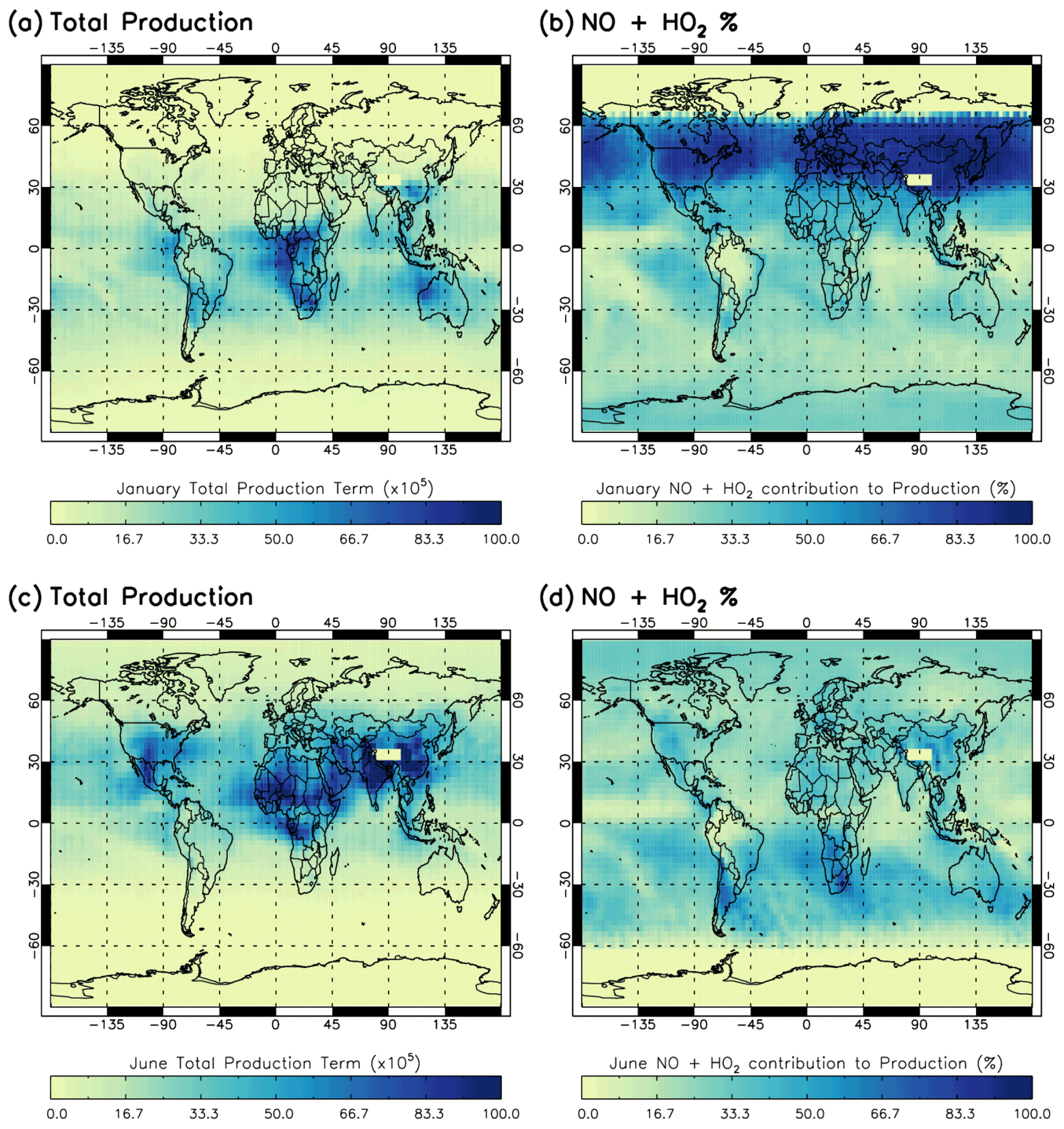
Figure 3 Contribution of NO + HO₂ reaction to total production term for Sav-SSA in 2010 averaged for the 600–700 hPa pressure region. (a) total production term in January, (b) percentage contribution of the NO + HO₂ source reaction to the total production term in January, (c) total production term in June and (d) percentage contribution of the NO + HO₂ source reaction to the total production term in June. Total production is in units of ×10⁵ molec. cm⁻³ s⁻¹.

Figures S13 and S14 show a comparison between [OH] calculated using the S-SSA, as in Eq. (4), but with the addition of one source term (NO + HO₂) and two sink terms (NO + OH + M and NO₂+ OH + M). The [OH] calculated using the NO_x terms shows an overestimate of between ∼0 and 4×10⁶ molec. cm⁻³ compared to TOMCAT [OH] for both January and June 2010 and improves the agreement in some regions, such as broadly above the Equator in January and below the Equator in June.

Although the NO + HO₂ source term is important in some regions, there are no NO or HO₂ satellite observations available in the relevant pressure range, so we cannot include this term in the S-SSA in this study. Introducing co-located tropospheric NO₂ satellite data from another instrument on MetOp-A, the Global Ozone Monitoring Experiment-2 (GOME-2), alongside IASI (Munro et al., 2016) is an area for potential future work. This would require additional steady-state balance expressions for NO : NO₂ and for HO₂.

Closer to the surface (>800 hPa), Figs. S15 and S16 show that there are a number of important sink reactions for OH which are not included in the S-SSA, but are included in the Sav-SSA. These sink species include nitrogen dioxide (NO₂), dimethyl sulfide (DMS), hydrogen (H₂), hydrogen peroxide (H₂O₂), NO, sulfur dioxide (SO₂), formaldehyde (HCHO) and a combination of hydrocarbons (e.g. alkanes and alkenes).

Figure 4 shows the regional impact of two VOC terms (of interest) on the total production term of the Sav-SSA, averaged across the 600–700 hPa pressure layer. The regional contribution of all sink terms can be found in the Supplement. Figure 4 shows that C₅H₈ (isoprene), from the sum of the hydrocarbon term, shows a large contribution across South America and Indonesia in both January and June. These are regions of high S-SSA OH compared to TOMCAT OH seen in Fig. 2, representing the lack of this sink term in the S-SSA, leading to an overestimation by the S-SSA. In these regions, the S-SSA expression is shown to not fully capture the OH chemistry. Formaldehyde (HCHO) represents ∼10 % of the total sink term in both months.

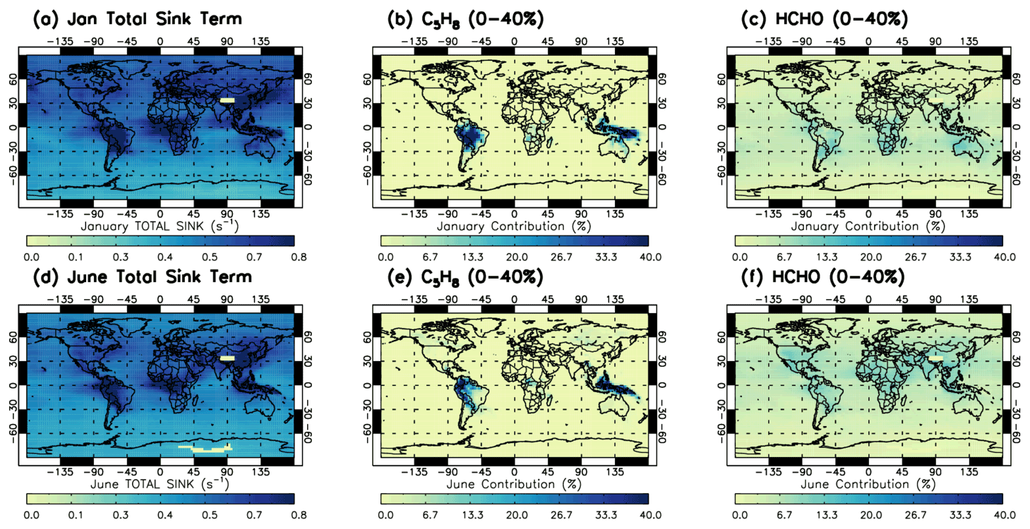
Figure 4 Contribution of isoprene (C₅H₈) and formaldehyde (HCHO) OH sink reactions to the total sink term for Sav-SSA in 2010 averaged for the 600–700 hPa pressure region. (a) Total sink term in January, (b) percentage contribution of the OH + C₅H₈ to the total sink term in January, (c) percentage contribution of the OH + HCHO to the total sink term in January, (d) total sink term in June, (e) percentage contribution of the OH + C₅H₈ to the total sink term in June and (f) percentage contribution of the OH + HCHO to the total sink term in June. Percentage value in panel label (i.e. 0 %–40 %) refers to the colour bar range. Total sink is in units of s⁻¹.

These additional source and sink terms could potentially help reduce the overestimate of the S-SSA in this region. Satellite data on tropospheric columns of NO₂ and several other relevant species (HCHO and SO₂ at enhanced levels) are available from GOME-2 alongside IASI on MetOp-A. Other than in tropical regions of lightning NO_x production and rapid convective uplift, these reside principally in the lower troposphere. Co-located data from GOME-2 could therefore allow further investigation in future work. For the other source and sink species, satellite data are either not available in the relevant pressure region or not available from a similar instrument to the species in the S-SSA. This would yield problems, such as in combining observations with different vertical resolutions at different locations and times of day.

Overall, the spatially varying importance of different source and sink terms prevents the S-SSA from achieving a spatially uniform agreement and this must be considered when applying the approximation.

3.1.3 Application to satellite data

We apply satellite-retrieved trace gas data and model j₁ for 2010 to estimate [OH] using the S-SSA in the layer of interest, between 600–700 hPa. The satellite profiles interpolated to this layer are applied on an individual sounding basis for the daytime (∼09:30 LST) overpass. The [OH] estimates are then gridded onto the model grid for comparisons. Figure 5 shows the satellite S-SSA [OH] for 2010. The mass-weighted global mean [OH] ranges from 2.1×10⁶ molec. cm⁻³ (January) to 2.9×10⁶ molec. cm⁻³ (July). The seasonal variation is clear, with the higher [OH] values above 5.0×10⁶ molec. cm⁻³ for example mostly in the SH during the summer (December–February), with a grid-box maximum value of 10.6×10⁶ molec. cm⁻³. These larger [OH] concentrations in the tropical region, between 30^∘ S–30^∘ N, appear from March to May, with a grid-box maximum of 10.9×10⁶ molec. cm⁻³. For June to August the higher [OH] values are mostly in the NH, with a grid-box maximum of 28.1×10⁶ molec. cm⁻³. The higher [OH] values are present around the Equator and sub-tropics in September to November, with a grid-box maximum of 11.4×10⁶ molecule cm⁻³.

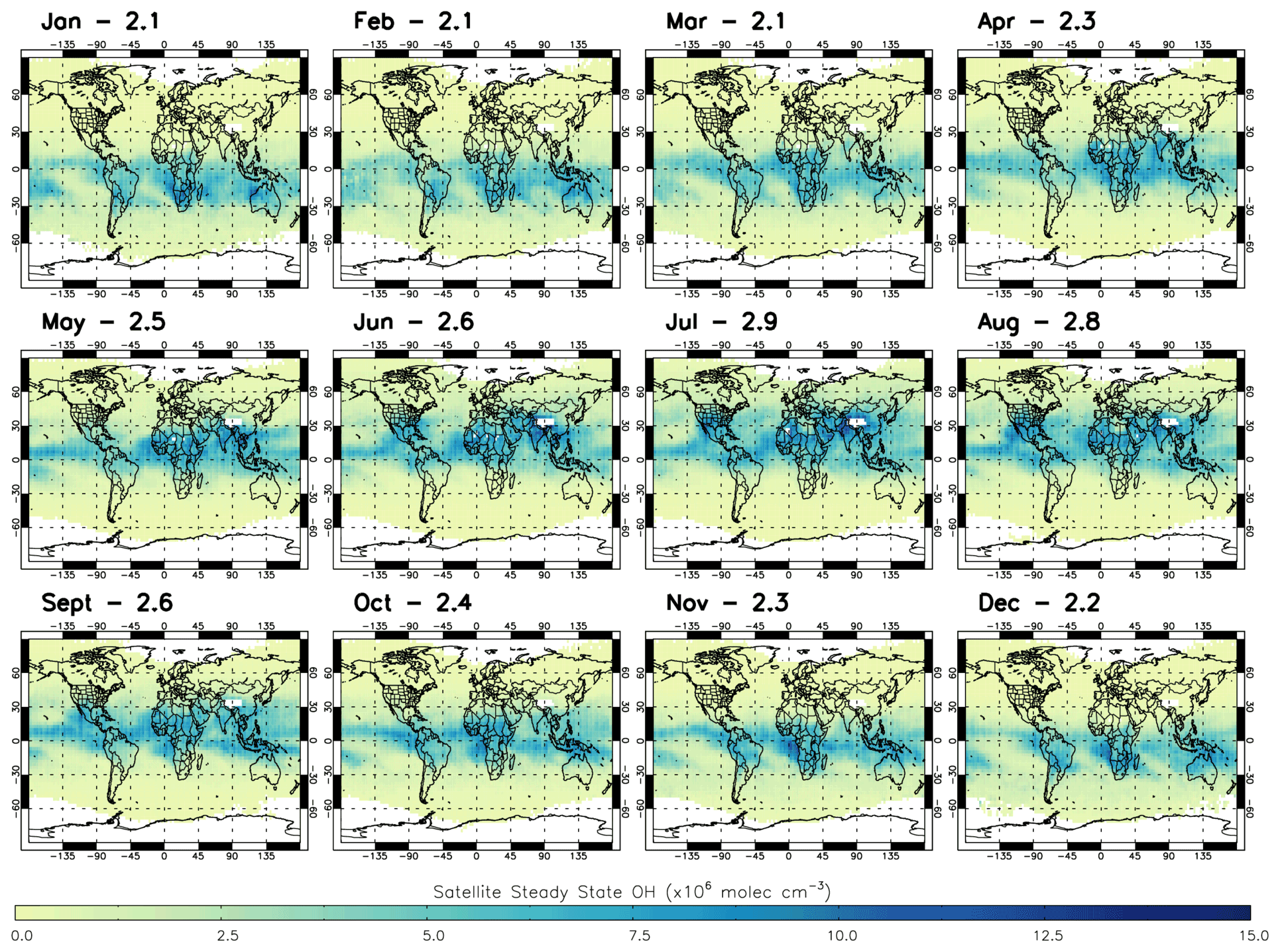
Figure 5 Satellite S-SSA OH (×10⁶ molec. cm⁻³) averaged for the 600–700 hPa layer in all months of 2010. Global mass-weighted mean OH values (×10⁶ molec. cm⁻³) for this region are labelled for each month.

Figure 6 shows a comparison of TOMCAT, TOMCAT S-SSA, TOMCAT FC-SSA and satellite S-SSA [OH] in January and June 2010. In both months the four estimates are seen to have very similar geographical structures. As expected, TOMCAT [OH] and TOMCAT FC-SSA [OH] show spatial patterns and global averages which are particularly similar (<6 % difference). This good agreement indicates that the use of monthly model data in the steady-state expression matches well with the numerical integration scheme inside the model. The TOMCAT and satellite S-SSA distributions also agree well in both months. The agreement is closer in January than June, with comparable peaks over NW Australia and southern Africa, with a TOMCAT [OH] grid-box maximum of 9.7×10⁶ molec. cm⁻³ and a satellite [OH] grid-box maximum of 10.3×10⁶ molec. cm⁻³. The TOMCAT and satellite S-SSA January global mean [OH] values are 2.85 and 2.21×10⁶ molec. cm⁻³, respectively, so are consistent to ∼22 %. In June 2010, TOMCAT and satellite S-SSA distributions have peaks over southern Asia and northern Africa. Over SE Asia, the TOMCAT and satellite peaks are ∼15 and 12×10⁶ molec. cm⁻³, respectively, and over northern Africa they are ∼15 and 8×10⁶ molec. cm⁻³, respectively. The TOMCAT distribution also has a peak over North America which is not captured by the satellite S-SSA. The TOMCAT and satellite S-SSA June global mean [OH] values are 3.80 and 2.73×10⁶ molec. cm⁻³, respectively, so are consistent to ∼28 %. The correlation coefficient between the monthly average grid boxes of TOMCAT and satellite S-SSA OH is 0.85 for January and 0.83 for June. In summary, the monthly-mean geographical distributions and global averages derived using the S-SSA (using TOMCAT/satellite data) agree well with those from TOMCAT and TOMCAT FC-SSA, indicating the S-SSA offers a useful approach to investigate [OH] behaviour globally in the 600–700 hPa layer. The monthly-mean distributions of satellite-derived S-SSA [OH] agree well with TOMCAT S-SSA, although values are generally lower, indicating some inconsistency between TOMCAT and the satellite in the distributions of H₂O, O₃, CO and/or CH₄. The same analysis was applied to data from 2017 (Fig. S10) and similar results were obtained, a global underestimate for the satellite S-SSA of 21 % in January and 28 % in June.

Figure 6 The 2010 OH comparison in the 600–700 hPa layer: (a) TOMCAT January, (b) TOMCAT June, (c) TOMCAT FC-SSA January, (d) TOMCAT FC-SSA June, (e) TOMCAT S-SSA January, (f) TOMCAT S-SSA June, (g) satellite S-SSA January and (h) satellite S-SSA June. Global mass-weighted mean OH values (×10⁶ molec. cm⁻³) for this atmospheric region are given below each panel.

3.2 Application to aircraft data

To further assess the robustness of the S-SSA, we apply it to CH₄, CO, O₃, H₂O and j₁ observations from four ATom campaigns. Figure 7 shows a comparison between [OH] observed by ATom (OH_obvs) and as calculated from ATom H₂O, O₃, CO and CH₄ observations using the S-SSA (OH_calc) where ATom data were available for all species. Across all four ATom campaigns, OH_calc is biased by −25.8 % with respect to OH_obvs. This bias is similar to the uncertainty on OH_obvs of ∼35 % (Brune et al., 2020). For the four individual campaigns, the percent bias is persistently negative, ranging from −21.1 % to −25.2 % for ATom-1,3,4 and −48.8 % for ATom-2. One explanation for the large normalised mean bias for ATom-2 is due to the predominance of smaller values of [OH] during this campaign, leading to higher percentage differences, as the absolute bias is more in line with the other campaigns. Across the four campaigns Pearson's correlation coefficient is 0.78, and for the four individual campaigns, the correlation ranges from 0.51 to 0.86.

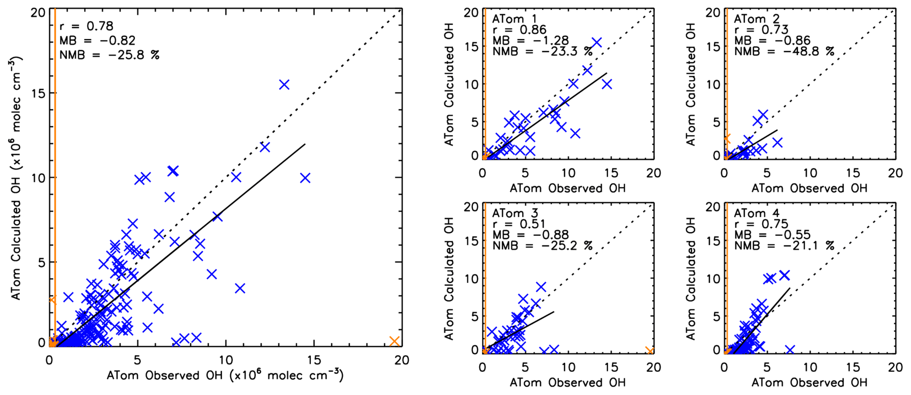
Figure 7 Comparison between OH_calc and OH_obvs. The left panel shows a combination of ATom-1, ATom-2, ATom-3 and ATom-4. The right four panels show the data split into the individual campaigns. ATom observations are filtered for 600–700 hPa and 08:00–11:00 LT. All data are in units of ×10⁶ molec. cm⁻³. Data points in orange are excluded from the analysis, either as an outlier ( $>\mathrm{mean}+\mathrm{3.0}$ standard deviations) or below the limit of detection of the ATHOS instrument (0.018 pptv or 0.31×10⁶ molec. cm⁻³) shown by the orange line. Pearson's correlation coefficient (r), the mean bias (calculated from OH_calc–OH_obvs) and the normalised mean bias (percent with respect to OH_obvs) are displayed in the top left corner of each panel.

Figure 8 shows a comparison between zonally averaged OH_obvs and OH_calc. The left panels show that for OH_obvs the higher values are predominantly found closer to the Equator, although exceptions exist around 45^∘ N in ATom-1. The right panels show that for the majority of latitudes, OH_obvs is larger than OH_calc across all four campaigns, with a few exceptions, mostly in ATom-2 and ATom-4. The deviations range from $-\mathrm{9.7}\times {\mathrm{10}}^{\mathrm{6}}$ to 4.1×10⁶ molec. cm⁻³. Generally, they are smallest between 30 and 90^∘ S, corresponding to the low OH_obvs and OH_calc values in this region. They are higher in 30^∘ S–30^∘ N and 30–90^∘ N, corresponding to generally higher OH_obvs and OH_calc values near the Equator and some large values in the NH mid-latitudes.

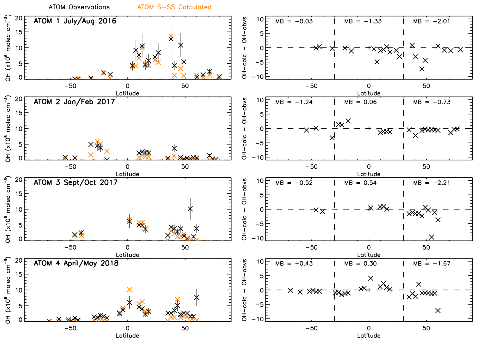
Figure 8 OH_calc and OH_obvs comparison. Left panels show latitude-averaged OH (ppt) with error bars of 35 %. Right panels show latitude-averaged OH difference between OH_calc and OH_obvs (calc–obvs) with the mean difference (MB) labelled for three different latitude regions marked by the dashed lines (90–30^∘ S, 30^∘ S–30^∘ N and 30–90^∘ N). All data are in units of ×10⁶ molec. cm⁻³. ATom observations are filtered for 600–700 hPa and 08:00–11:00 LT.

The normalised mean bias between OH_obvs and OH_calc is ∼26 %, which is a similar order of magnitude to the large uncertainty of 35 % for the OH observations. The ATom observations provide a comparatively large aircraft dataset for comparison; however, it nonetheless has a limited spatiotemporal extent, which must be acknowledged when interpreting our results. Here, we believe that for the observations used, the datasets are correlated sufficiently to justify further study of the S-SSA at this pressure range.

Figure 9 shows OH_obvs overlaid onto a satellite-derived [OH] field averaged across the corresponding days in 2017. The comparison is challenging due to the sparse nature of the ATom data points compared to the satellite [OH] field (highlighted in Fig. 9) and using satellite data only for 2017 (ATom-1 occurred in 2016 and ATom-4 in 2018). There are examples of good agreement between the satellite and OH_obvs in some peak-[OH] regions, e.g. off the western coast of Mexico between the Equator and 30^∘ N in ATom-1, and also low [OH] regions, e.g. over the North Atlantic Ocean in ATom-2. However, there are also examples of poor agreement, e.g. high values in OH_obvs near Alaska and low values in the satellite OH in ATom-3 and ATom-4. Across the four campaigns, the correlation coefficient ranges from 0.15 to 0.75, and the bias of satellite with respect to ATom ranges from −60.1 % to −35.1 %. The poor comparison in some regions may be attributable to the resolution difference between the point aircraft observations and the averaged satellite [OH] field, due to spatial inhomogeneity of OH.

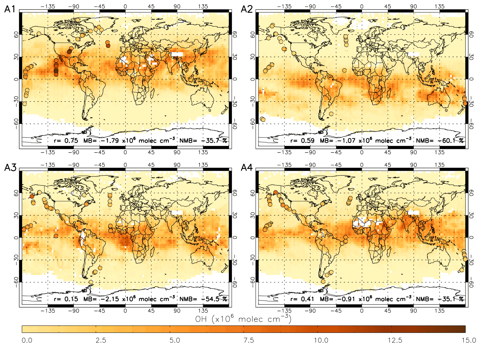
Figure 9 Satellite OH for four periods in 2017 corresponding to A1 to A4 (ATom-1 to ATom-4, 2016–2018) with ATom OH observations (OH_obvs) overlaid on top as coloured circles. ATom observations are filtered for 600–700 hPa and 08:00–11:00 LT. Pearson's correlation coefficient (r), mean bias (calculated from the nearest satellite grid cell – OH_obvs) and the normalised mean bias (percent with respect to OH_obvs) are displayed at the bottom of each panel. All data are in ×10⁶ molec. cm⁻³.

Figure 10 shows a comparison between OH_obvs and the nearest value from the averaged satellite [OH] field (OH-sat). The data are coloured by latitude and, as in Fig. 9, indicate OH-sat to be negatively biased with respect to OH_obvs at northern middle–high latitudes, but to a lesser extent at lower latitudes. Across the four campaigns, the values at northern middle–high latitudes (30–90^∘ N) and the values at lower latitudes (90^∘ S–30^∘ N) show similarly high correlation coefficients of 0.68, with a small difference of 9.4 % for the lower latitudes and a much larger difference of 72.8 % for the higher latitudes. This corresponds to the results in Sect. 3.1.2, where the OH source reaction HO₂+ NO represents a larger contribution to the total production in the NH high latitudes in winter (ATom-2, ATom-3 and ATom-4). The reduction in agreement in this region indicates that the S-SSA may not be able to provide robust information about [OH] here. In Sect. 3.3 we study a tropical (15^∘ S–15^∘ N) band, where the S-SSA shows a more robust agreement.

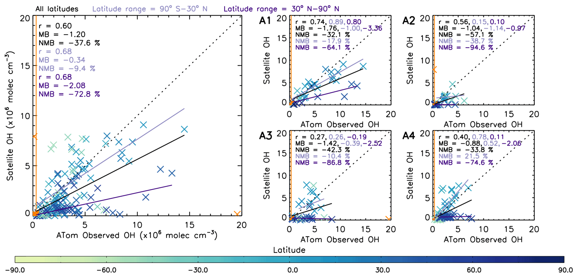
Figure 10 Comparison between OH_obvs and OH-sat (nearest satellite OH value to ATom observation from averaged 2017 satellite OH grid). The left panel shows a combination of ATom-1, ATom-2, ATom-3 and ATom-4. The right four panels show the data split into the individual campaigns. ATom observations are filtered for 600–700 hPa and 08:00–11:00 LT. All data are in units of ×10⁶ molec. cm⁻³. Data points in orange are not included in analysis, either as an outlier ( $>\mathrm{mean}+\mathrm{3.0}$ standard deviations) or below the limit of detection of the ATHOS instrument (0.018 pptv or 0.31×10⁶ molec. cm⁻³) shown by the orange line. Pearson's correlation coefficient (r), the mean bias (calculated from OH-sat – OH_obvs) and the normalised mean bias (percent with respect to OH_obvs) are displayed in the top left corner of each panel for three different latitude ranges: all latitudes, 90^∘ S–30^∘ N and 30–90^∘ N. The values are coloured by latitude as shown on the colour bar.

Aircraft data and omitted source terms

Figure S17 is similar to Fig. 7 but shows a comparison of ATom OH_calc with (OH_calc-NO_x) and without (OH_calc) three NO_x reactions (NO + HO₂, NO + OH + M, NO₂+ OH + M) included in the S-SSA. The addition of the NO_x terms changes the bias in the OH_calc relative to OH_obvs from −20.6 % to +13.2 %. This change in sign is consistent with the comparison of S-SSA and S-SSA, with NO_x reactions using model data as shown in Figs. S13 and S14. Overall, the correlation remains similar with and without NO_x (0.76 and 0.78). This corresponds to the model results in Sect. 3.1.2, which show that for some regions, the NO + HO₂ source term can make a large contribution to the total source term.

3.3 OH reactivity

As described in Sect. 2.2, OHR observations can potentially be used to check the denominator of a steady-state approximation, in this case a simplified expression of OHR (Eq. 5). Section S10 (Figs. S18 and S19) discusses our comparisons between ATom OHR observations (OHR-obvs) and ATom data used in the simplified expression for OHR (OHR-calc). Although ∼80 % of calculated OHR values fell within the range of measurement uncertainty, the estimated error on OHR measurements (0.8 s⁻¹) was too large to find any correlation with calculated OHR ($r=-\mathrm{0.02}$). The bias in calculated OHR varied between −57 % and +20 % over the four campaigns, and the average bias in calculated OHR (−37 %) over the four campaigns (Fig. S18) is compatible with the (−28 %) bias in S-SSA [OH]. Several studies (Thames et al., 2020; Travis et al., 2020) have quantified “missing OH reactivity” in the boundary layer in detail; however, our analysis of ATom [OH] and OHR measurements demonstrates the S-SSA to estimate [OH] with an accuracy within ∼30 % in the 600–700 hPa layer.

3.4 OH temporal variation

Satellite data in conjunction with the S-SSA presented in previous sections provide a means to examine the temporal variation in global [OH]. We use satellite data produced on a sub-sampled basis from 2008–2017 and the S-SSA, together with fixed monthly model j₁ distributions from the TOMCAT model for a fixed year (2010). The use of a fixed year of j₁ distributions removes any influence from variation in this value between years, e.g. from variation in overhead stratospheric ozone, which is an assumption that should be considered when interpreting these results. Figure 11 shows the time series of global, NH, SH and tropical (15^∘ S–15^∘ N) OH monthly anomalies with respect to the 2008–2017 mean for each month for the 600–700 hPa layer. We include a tropical band as this is the most representative region of OH using the S-SSA. Similar plots in Sect. S11 show percent anomalies for the input species and temperature (Figs. S20–S24). During this time period the [OH] anomaly varies between −0.10 and $+\mathrm{0.15}\times {\mathrm{10}}^{\mathrm{6}}$ molec. cm⁻³ for the global average, −0.15 and $+\mathrm{0.11}\times {\mathrm{10}}^{\mathrm{6}}$ molec. cm⁻³ for the NH average, −0.21 and $+\mathrm{0.21}\times {\mathrm{10}}^{\mathrm{6}}$ molec. cm⁻³ for the SH average, and −0.37 and $+\mathrm{0.54}\times {\mathrm{10}}^{\mathrm{6}}$ molec. cm⁻³ for the tropical average. Aside from a few exceptions, the global, NH, SH and tropical averages follow a similar pattern. Notable positive anomalies (values given for the tropical band, in units of ×10⁶ molec. cm⁻³) occur in mid-2010 (+0.30), the end of 2012 and beginning of 2013 (+0.54), mid-2015 (+0.15), and mid-2016 (+0.14). Notable negative anomalies occur in mid-2009 (−0.27), 2011 to mid-2012 (−0.37), the end of 2015 and beginning of 2016 (−0.21), and the end of 2017 (−0.22). The global annual mean [OH] anomaly ranges from −3.1 % to +4.7 %, and the tropics anomaly ranges from around −6.9 to +7.7 %. This behaviour is broadly similar to other studies of [OH] variability using MCF observations and chemistry transport models, which find a range of around −6 to +6 % for global [OH] anomaly during this time period (although our assessment is limited to a specific pressure range, so this is not a direct comparison; Voulgarakis et al., 2015; Patra et al., 2021).

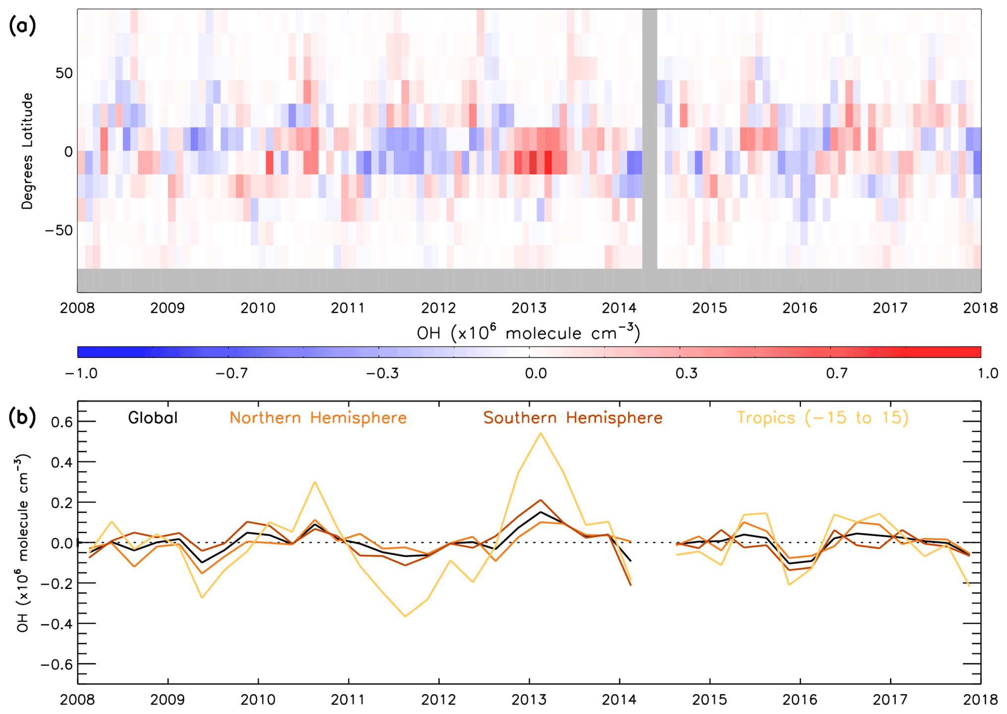
Figure 11 Monthly mean satellite OH anomaly (2008–2017): (a) 15^∘ latitude bins and (b) 3-month average global, NH, SH and tropics means. All data are in ×10⁶ molec. cm⁻³. Anomaly is relative to a 2008–2017 average.

Figure 12 shows contrasting behaviour of the three sink terms during the time period 2008–2017. It shows that in the 600–700 hPa layer, CO is the dominant sink term, ranging between 0.20–0.45 s⁻¹, with the CH₄ sink having the next largest contribution between 0.10–0.15 s⁻¹ and the O₃ sink having the smallest contribution at around 0.04 s⁻¹. The comparatively large size of the CO sink indicates that variation in CO is likely to dominate the variation in the total sink term. The CO sink is consistently lower in the SH than NH, with the largest difference (∼0.2 s⁻¹) in the first half of the year. The CH₄ and O₃ sinks show a negligible difference between SH and NH; therefore the CO sink will have a lower percentage contribution in the SH. These findings are consistent with those from aircraft measurements below 3 km in Travis et al. (2020) and from model data in the free troposphere in Lelieveld et al. (2016). Satellite CH₄ shows a positive trend of 4.5 ppb yr⁻¹ throughout this time period (Fig. S21). However, as seen in Fig. 12, when the rate constant is applied, the CH₄ sink term shows very little variation, with no evidence of the positive trend in CH₄ concentrations having a significant impact. The source term (numerator of Eq. 4) varies between 5–15×10⁵ molec. cm⁻³ s⁻¹ for the global, NH and SH averages, while for the tropical band it ranges between 15–28×10⁵ molec. cm⁻³ s⁻¹.

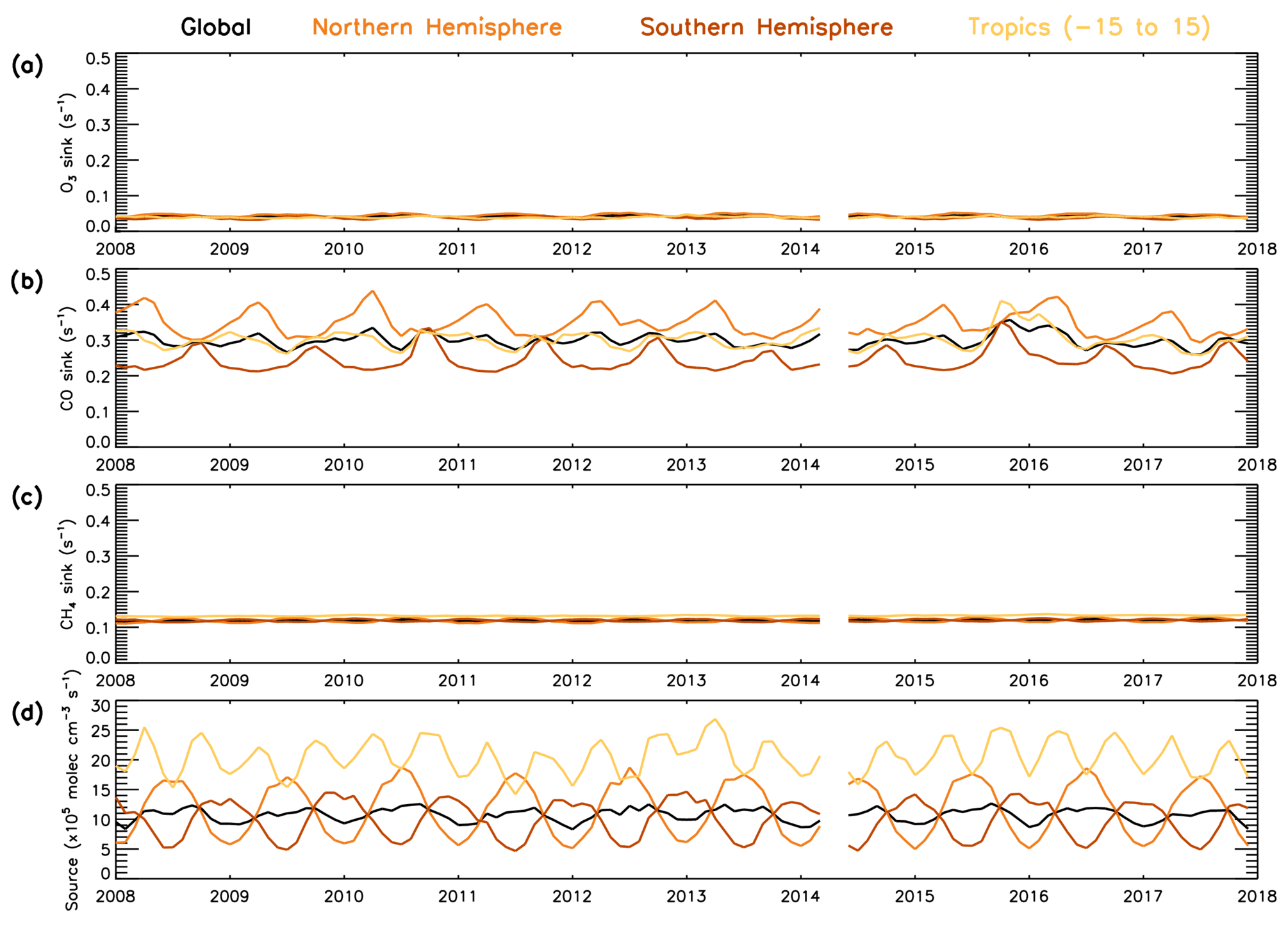
Figure 12 Temporal variability in the components of the S-SSA approximation (2008–2017). Global, NH, SH and tropical average time series for (a) $k_{{\mathrm{O}}_{\mathrm{3}}+\mathrm{OH}}$[O₃], (b) k_CO+OH[CO], (c) $k_{{\mathrm{CH}}_{\mathrm{4}}+\mathrm{OH}}$[CH₄] and (d) 2j₁k₁[O₃][H₂O]/($k_{{\mathrm{N}}_{\mathrm{2}}+\mathrm{O}\left({}^{\mathrm{1}}\mathrm{D}\right)}$[N${}_{\mathrm{2}}]+k_{{\mathrm{O}}_{\mathrm{2}}+\mathrm{O}\left({}^{\mathrm{1}}\mathrm{D}\right)}$[O${}_{\mathrm{2}}]+k_{{\mathrm{H}}_{\mathrm{2}}\mathrm{O}+\mathrm{O}\left({}^{\mathrm{1}}\mathrm{D}\right)}$[H₂O]).

Figure 13 shows the temporal anomaly, relative to the 2008–2017 mean, of the balance between source and sink terms in the approximation and the derived OH concentration. The positive anomalies in mid-2010, the end of 2012 and beginning of 2013, mid-2015, and mid-2016 coincide with the positive anomalies in the source term, driven by O₃ (O₃ anomalies are shown in Fig. S23), and they are smaller than or close to zero anomalies in the sink terms. The negative anomalies in mid-2009, 2011 to mid-2012, and the end of 2017 can be explained by a negative anomaly in the source term, again driven by O₃, and a small or close-to-zero anomaly in the sink term. The negative anomalies at the end of 2015 and beginning of 2016 can be explained by a very large positive sink term anomaly, despite the large positive source term anomaly. This large positive anomaly in the sink term corresponds to a large positive anomaly of CO in most latitudes (Fig. S22), with a maximum anomaly of ∼12 % globally and ∼20 % in the tropics. The 2015–2016 El Niño event is the likely cause of this CO anomaly, due to a large increase in global fire emissions (Huijnen et al., 2016). As shown in Fig. 13d, the event started at the end of 2014, peaked at the end of 2015 with a maximum multivariate ENSO index (MEI.v2) value of +2.2 and ended in May 2016 (Liu et al., 2017; NOAA, 2021). Biomass burning was also found to be the key driver of OH variability in a study by Voulgarakis et al. (2015).

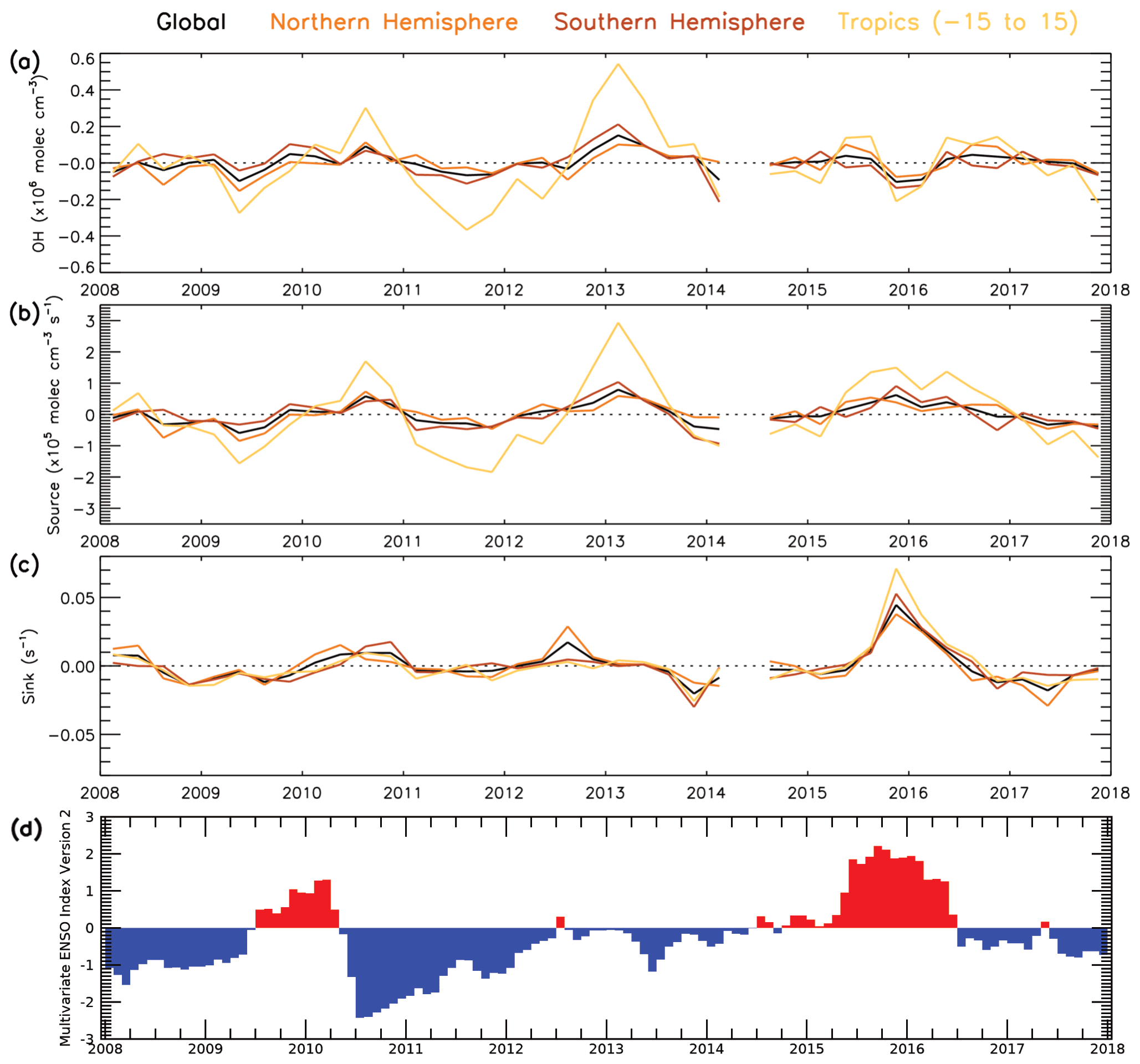
Figure 13 Temporal variability in OH anomaly and anomalies of the numerator (source) and denominator (sink) lines of the steady-state approximation in Eq. (4) (2008–2017). Global, NH, SH and tropical average time series for (a) OH anomaly, (b) 2j₁[O₃][H₂O]$/$($k_{{\mathrm{N}}_{\mathrm{2}}+\mathrm{O}\left({}^{\mathrm{1}}\mathrm{D}\right)}$[N₂]$+k_{{\mathrm{O}}_{\mathrm{2}}+\mathrm{O}\left({}^{\mathrm{1}}\mathrm{D}\right)}$[O₂]$+k_{{\mathrm{H}}_{\mathrm{2}}\mathrm{O}+\mathrm{O}\left({}^{\mathrm{1}}\mathrm{D}\right)}$[H₂O]) (total source term) anomaly, (c) k_CO+OH[CO] $+k_{{\mathrm{CH}}_{\mathrm{4}}+\mathrm{OH}}$[CH₄] $+k_{{\mathrm{O}}_{\mathrm{3}}+\mathrm{OH}}$[O₃] (total sink term) anomaly and (d) bimonthly multivariate ENSO index (NOAA, 2021). Anomalies are relative to a 2008–2017 average.

As the combined source term is a dominant driver of OH variability, it is useful to distinguish the relative importance of O₃ and water vapour in driving this variability. To do this, we repeat the source term calculation (numerator in Eq. 4) but using a fixed value of O₃ or water vapour. These fixed values are derived from the average value for each month across the full 2008–2017 time series. If the source term anomaly time series derived using a fixed water vapour value can reproduce the original anomaly time series (i.e. Fig. 13b), this would demonstrate that variability of water vapour is not important in comparison to that of O₃ or vice versa (Fig. 14). Our results show that when water vapour is fixed (varying O₃) in the source term anomaly, 66.4 % of the variability (i.e. R²=0.664) in the original source term can be explained on the global scale (Fig. 14c). When O₃ is fixed to a constant monthly value (varying water vapour), the R² value drops to 0.164 with only 16.4 % of the variability in the original source term anomaly explained by this time series (Fig. 14b). This demonstrates that variations in O₃ are the primary driver in the source term and therefore in the OH variability using the S-SSA in this altitude range and time period. Cross-correlations between the drivers of the key species OH, O₃, are likely to exist; however a detailed analysis and quantification of this is beyond the scope of the study.

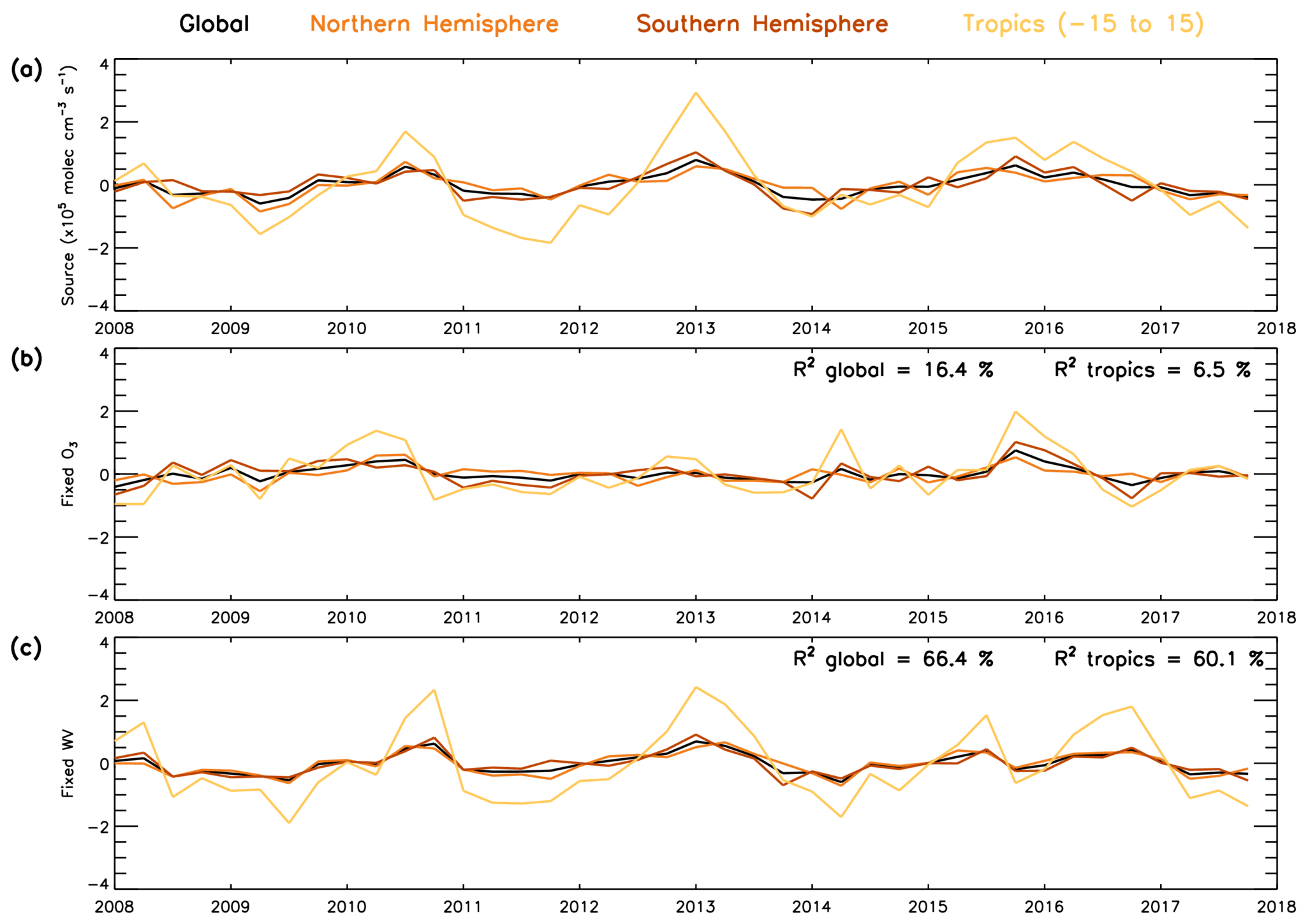
Figure 14 Global, NH, SH and tropical average time series (2008–2017) for (a) OH S-SSA source anomaly, (b) OH S-SSA source anomaly calculated with fixed monthly O₃ concentrations (source fixed-O₃) and (c) OH S-SSA source anomaly calculated with fixed monthly water vapour concentrations (source fixed-wv). Fixed O₃ and water vapour calculated as monthly average across the time period. Anomalies are relative to a 2008–2017 average. Values in the top right of panel (b) represent the R² value between the OH S-SSA source anomaly and the source fixed-O₃ anomaly, and values in the top right of panel (c) represent the R² values between the OH S-SSA source anomaly and the source fixed-wv anomaly. All data are in units of ×10⁵ molec. cm⁻³ s⁻¹.

4 Conclusions

Due to its short photochemical lifetime, steady-state approximations are able to represent tropospheric OH concentrations well, depending on the complexity of the expression used and the atmospheric pressure range over which they are applied. The terms in the steady-state approximation also allow us to quantify components which contribute to the OH budget. A simplified steady-state approximation (S-SSA) can be constructed which contains terms based on trace gases observed by satellite. Results from the TOMCAT 3D chemical transport model show that this should be a good approximation to [OH] in the 600–700 hPa layer in terms of magnitude (∼26 %–31 % underestimate in the mass-weighted global mean [OH] comparison to full chemistry) and spatial distribution. This atmospheric layer is above the boundary layer where [OH] is substantially affected by many pollutants which are not measured by satellite and therefore invalidate the S-SSA. We have tested the S-SSA in the 600–700 hPa layer using data from four ATom aircraft campaigns and found that it tracked measured [OH] with a correlation of r=0.78 and a mean bias of ∼26 %, similar to the 35 % estimated uncertainty on the OH observations. Measurements of OH reactivity (OHR) allow the denominator of the S-SSA expression to be considered in addition and found to be consistent with an S-SSA [OH] accuracy of ∼30 % in the 600–700 hPa layer.

The S-SSA approach allows us to demonstrate how a multi-year record of satellite observations can be used to examine interannual variability in tropospheric [OH]. Using H₂O, O₃, CO and CH₄ data retrieved from MetOp-A observations for 2008–17 we find the global annual mean [OH] anomaly to range from −3.1 % to +4.7 %. The influence of important terms in the OH budget was also derived, demonstrating the balance between the source and sink terms over time. Variation in the S-SSA OH was found to be determined primarily by the combined source term, driven by O₃, and by the CO sink term. In the tropics, OH variation reflected that of O₃ (peaks in 2008, 2010 and the largest in 2013) along with the positive CO anomaly associated with the strong El Niño event in 2015/16. Overall, we have demonstrated a novel and robust methodology, using satellite observations and a simple steady-state approach, to estimate mid-troposphere [OH], which can complement existing methods to measure [OH] (i.e. the limited network of surface sites, infrequent flight campaigns and the MCF-type approach to estimate global mean [OH]). Most importantly though, the approach here will provide the scientific community with a global observational constraint on mid-tropospheric [OH] and help future studies assess the [OH] impacts on important air quality (e.g. O₃ and NO₂) and climate (e.g. CH₄) trace gases.