Ozone–gravity wave interaction in the upper stratosphere/lower mesosphere

The increase in amplitudes of upward propagating gravity waves (GWs) with height due to decreasing density is usually described by exponential growth. Recent measurements show some evidence that the upper stratospheric/lower mesospheric gravity wave potential energy density (GWPED) increases more strongly during the daytime than during the nighttime. This paper suggests that ozone–gravity wave interaction can principally produce such a phenomenon. The coupling between ozone-photochemistry and temperature is particularly strong in the upper stratosphere where the time–mean ozone mixing ratio decreases with height. Therefore, an initial ascent (or descent) of an air parcel must lead to an increase (or decrease) in ozone and in the heating rate compared to the environment, and, hence, to an amplification of the initial wave perturbation. Standard solutions of upward propagating GWs with linear ozone–temperature coupling are formulated, suggesting amplitude amplifications at a specific level during daytime of 5 % to 15 % for low-frequency GWs (periods ≥4 h), as a function of the intrinsic frequency which decreases if ozone–temperature coupling is included. Subsequently, the cumulative amplification during the upward level-by-level propagation leads to much stronger GW amplitudes at upper mesospheric altitudes, i.e., for single low-frequency GWs, up to a factor of 1.5 to 3 in the temperature perturbations and 3 to 9 in the GWPED increasing from summer low to polar latitudes. Consequently, the mean GWPED of a representative range of mesoscale GWs (horizontal wavelengths between 200 and 1100 km, vertical wavelengths between 3 and 9 km) is stronger by a factor of 1.7 to 3.4 (2 to 50 J kg⁻¹, or 2 % to 50 % in relation to the observed order of 100 J kg⁻¹, assuming initial GW perturbations of 1 to 2 K in the middle stratosphere). Conclusively, the identified process might be an important component in the middle atmospheric circulation, which has not been considered up to now.

1 Introduction

Atmospheric gravity waves (GWs), with horizontal wavelengths of 100 to 2000 km, are produced in the troposphere and propagate vertically through the stratosphere and mesosphere, where gravity wave breaking processes are important drivers of the middle atmospheric circulation (e.g., Andrews et al., 1987; Fritts and Alexander, 2003). Usually, upward propagating GWs are described by sinusoidal wave perturbations in a slowly varying background flow of an exponentially growing amplitude with height due to decreasing density ($\sim e^{z/\mathrm{2}H}$, where H is the scale height). Recently, Baumgarten et al. (2017) found some evidence that the growth of the GW amplitudes between the middle stratosphere and upper mesosphere might be stronger during the daytime than during nighttime. The aim of the present paper is to examine whether ozone–gravity wave interaction can principally produce such an amplification.

Seasonal variations of gravity wave potential energy density (GWPED) have been derived based on satellite data or lidar measurements (e.g., Geller et al., 2013; Ern et al., 2004, 2018; Kaifler et al., 2015; Baumgarten et al., 2017). At summer middle and polar latitudes, the order of the monthly mean GWPED increases from approximately 1 J kg⁻¹ in the middle stratosphere (30–40 km) to 10 J kg⁻¹ in the lower mesosphere (50–60 km) and 100 J kg⁻¹ in the upper mesosphere (80–90 km), with usual initial GW perturbations in the middle stratosphere in the order of about 1 to 2 K, and wave periods primarily between 4 to 10 h (e.g., Kaifler et al., 2015; Baumgarten et al., 2017, 2018; Ern et al., 2018). Generally, the GW sources in the middle stratosphere are weaker, but the relative increase in the GWPED between the middle stratosphere and upper mesosphere are much stronger in summer than in winter, including a less pronounced seasonal cycle in the upper mesosphere than in the levels below. This is primarily due to the seasonal change in critical level filtering of the GWs by the zonal wind (e.g., Kaifler et al., 2015; Ern et al., 2018), but also due to specific GWs generated by convection and propagating towards polar latitudes (Chen et al., 2019), or to additional sources of GWs in the mesosphere, independent of the GWs at lower levels (Reichert et al., 2021). Recently, model simulations with resolved GWs suggested multistep vertical coupling processes, producing such secondary GWs as a result of dissipating primary GWs, which can strongly enhance the GW amplitudes in the upper mesosphere (e.g., Becker and Vadas, 2018; Vadas et al., 2018; Vadas and Becker, 2018). However, the potential role of daytime–nighttime differences in the increase in GW amplitudes with height have been considered only very sparsely up to now.

Baumgarten et al. (2017) derived monthly means of the GWPED from full-day lidar temperature measurements at northern mid-latitudes (54^∘ N, 12^∘ E), and found a stronger relative increase between 35 and 40 km and between 55 and 60 km for full-day than nighttime observations during summer months, but less pronounced differences during winter. For example, for July, the GWPED at 55–60 km show values of about $\mathrm{1}\times {\mathrm{10}}^{-\mathrm{2}}$ J m⁻³ (or 10 J kg⁻¹) for full-day measurements but about 0$.5\times {\mathrm{10}}^{-\mathrm{2}}$ J m⁻³ for nighttime only (or 0.2 but 0.1 J m⁻³, if the measured temperature fluctuations are vertically filtered for vertical wavelengths L_m<15 km), where the GWPED at 35–40 km remains nearly unchanged, indicating a difference between full-day and nighttime values by a factor of about 2. Generally, measurements of the mesospheric GWPED are much more uncertain during summer than winter months (e.g., Kaifler et al., 2015; Ehard et al., 2015; Baumgarten et al., 2017), and the signal-to-noise ratio of the lidar measurements is not as good during the daytime than during nighttime (e.g., Rüfenacht et al., 2018), which can stimulate some doubt on the reliability of the daytime–nighttime differences derived from these specific measurements. In addition, taking the potential uncertainties of the analyzing methods into account (i.e., the temporal filtering methods used for the measured time series), Baumgarten et al. (2017) speculated that a change in the phase of long periodic waves (e.g., diurnal and semidiurnal tides) could change the filtering conditions for GWs. However, Baumgarten et al. (2017) conclusively assumed that the detected daytime–nighttime differences are of true geophysical origin, where an unequivocal explanation of this phenomenon remained open. Considering also that the full-day observations of Baumgarten et al. (2018) during May 2016 showed pronounced GW activity, particularly at altitudes between 42 and 50 km where the coupling between ozone and temperature is particularly strong, it seems to be worthwhile to examine whether ozone–gravity wave interaction could principally lead to such daytime–nighttime differences in the GW amplitudes. This must then also lead to a potential effect on the differences in the GWPED between polar day and polar night. The examination of the present paper is based on standard equations describing upward propagating GWs in a constant background flow, excluding other processes controlling the GWPED variability, to provide a clear understanding and quantification of the potential effect, which cannot be achieved based on observational data analysis or comprehensive model calculations alone.

The coupling of temperature and ozone is particularly strong in the upper stratosphere due to the short photochemical lifetime of ozone (e.g., Brasseur and Solomon, 1995). Linear relationships for a change in the heating rate due to a change in ozone, and a change in photochemistry due to a change in temperature, were derived from basic theory or satellite observations, and have been introduced in standard equations of stratospheric dynamics to examine the effects on the stratospheric circulation, planetary-scale wave patterns, and equatorial Kelvin waves (Dickinson, 1973; Douglass et al., 1985; Froidevaux et al., 1989; Cordero et al., 1998; Cordero and Nathan, 2000; Nathan and Cordero, 2007; Ward et al., 2000; Gabriel et al., 2011a). Large-scale ozone-dynamic coupling processes also show significant effects in numerical weather prediction (NWP) or general circulation models (GCMs) (Cariolle and Morcrette, 2006; Gabriel et al., 2007, 2011b; Gillet et al., 2009; Waugh et al., 2009; McCormack et al., 2011; Albers et al., 2013). However, possible effects of mesoscale ozone–gravity wave interaction in the upper stratosphere/lower mesosphere (USLM) have not been considered up to now.

The basic idea of the present paper can be summarized as follows: in the USLM, the time–mean ozone mixing ratio μ₀(z) decreases with height ($\partial {\mathit{\mu }}_{\mathrm{0}}/\partial z<\mathrm{0}$). Therefore, at a specific level in the ULSM, an ascending air parcel initially forced by an upward propagating sinusoidal GW pattern (i.e., the wave crest with vertical velocity perturbation $w^{\prime }>\mathrm{0}$) must lead to an increase ($\partial {\mathit{\mu }}^{\prime }/\partial t>\mathrm{0}$) by both transport (because $-w^{\prime }\partial {\mathit{\mu }}_{\mathrm{0}}/\partial z>\mathrm{0}$) and photochemistry (because the temperature-dependent ozone production increases in the case of adiabatic cooling), and, hence, in the heating rate ($Q^{\prime }\left({\mathit{\mu }}^{\prime }\right)>\mathrm{0}$), comparable to the latent heat release in the troposphere in the case of condensation. Then, the induced perturbation ($\mathrm{\Delta }{\mathit{\theta }}^{\prime }>\mathrm{0}$, where θ is potential temperature) reinforces the initial ascent, where the lapse rate ($\partial ({\mathit{\theta }}_{\mathrm{0}}+\mathrm{\Delta }{\mathit{\theta }}^{\prime })/\partial z<\partial {\mathit{\theta }}_{\mathrm{0}}/\partial z$) decreases ($\partial z=$ constant), suggesting an effective ozone adiabatic lapse rate in the upper stratosphere comparable to the moist adiabatic lapse rate in the troposphere. Analogously, a descending air parcel (the wave trough where $w^{\prime }<\mathrm{0}$) leads to a decrease ($\partial {\mathit{\mu }}^{\prime }/\partial t<\mathrm{0}$) and a corresponding change ($Q^{\prime }\left({\mathit{\mu }}^{\prime }\right)<\mathrm{0}$), reinforcing the initial descent. Overall, this process must lead to a significant amplification of the initial GW amplitude at this level, and, hence, to a successive amplification of the amplitude during the upward level-by-level propagation through the ULSM.

In Sect. 2, standard equations for GWs in a zonal mean background flow with and without linearized ozone–temperature coupling are formulated to quantify the amplitude amplification at a specific level (or altitude) and latitude. Then, in Sect. 3, the cumulative amplitude amplification during the propagation through the USLM is derived, based on an idealized approach of the upward level-by-level propagation of GWs with specific horizontal and vertical wavelengths. Section 4 concludes with a summary and discussion.

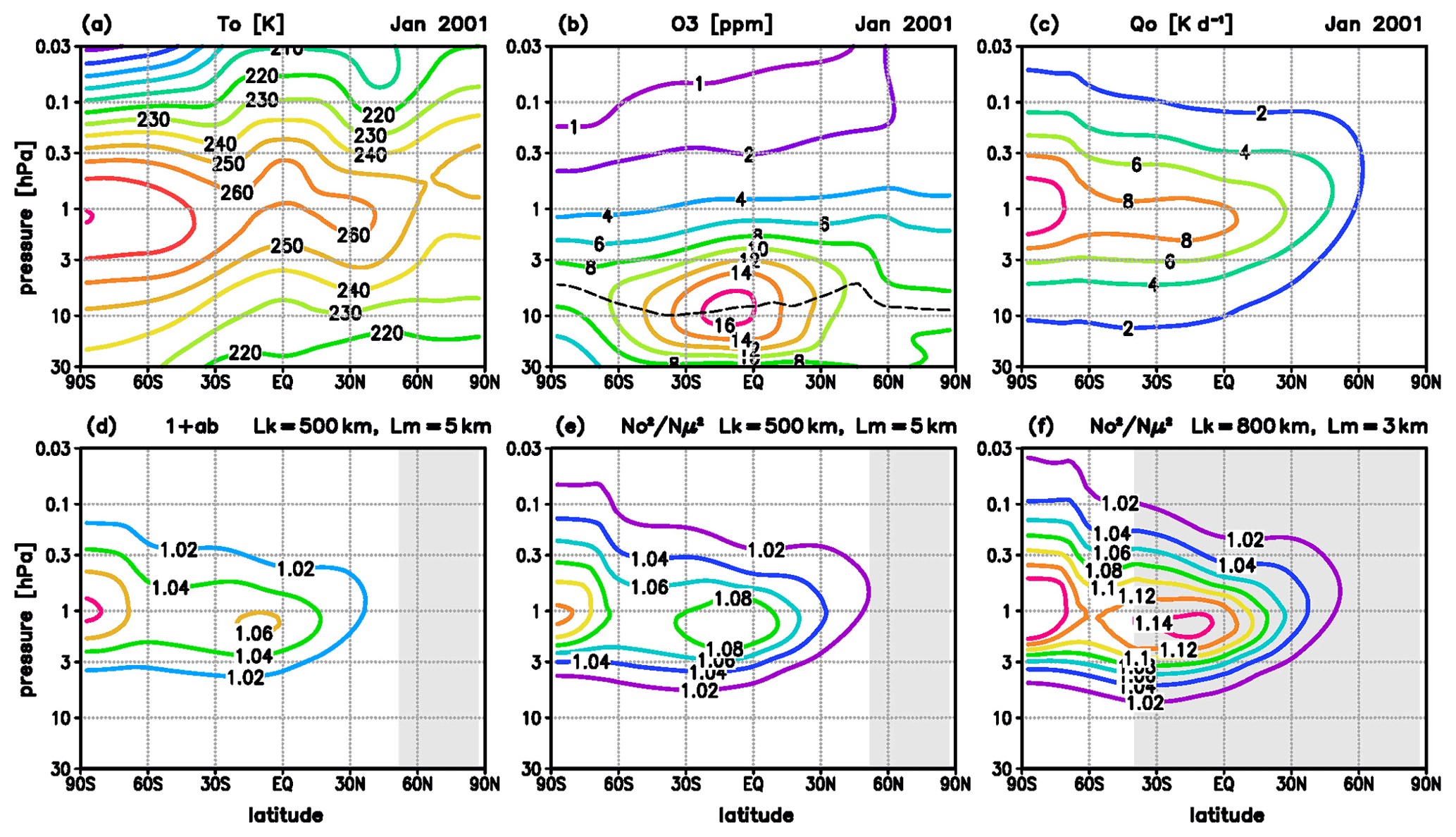
Figure 1 (a–c) Zonal and monthly mean background, (a) temperature T₀, (b) ozone mixing ratio O₃ (the dashed line denotes where ∂O${}_{\mathrm{3}}/\partial z=\mathrm{0}$), and (c) ozone heating rate Q₀, January 2001, extracted from a simulation with the circulation and chemistry model HAMMONIA; (d–f) amplification factors, (d) 1+ab and (e) $N_{\mathrm{0}}^{\mathrm{2}}/N_{\mathit{\mu }}^{\mathrm{2}}$ for a GW with horizontal and vertical wavelengths L_k=500 km and L_m=5 km, and (f) $N_{\mathrm{0}}^{\mathrm{2}}/N_{\mathit{\mu }}^{\mathrm{2}}$ for a GW with L_k=800 km and L_m=3 km; shaded areas denote the latitudes where the amplification is limited by the length of daylight (τ_i>τ_day).

2 Ozone–gravity wave interaction

In the following section, ozone–gravity wave interaction is analyzed based on standard equations describing GWs in a background atmosphere, where the solutions are illustrated for southern summer conditions. The background is prescribed by monthly and zonal mean temperature T₀, ozone μ₀, and short-wave heating rate Q₀ of January 2001 (Fig. 1a–c), derived from a simulation with the high-altitude general circulation and chemistry model HAMMONIA (details of the model are given by Schmidt et al., 2010). The heating rate Q₀ (Fig. 1c) is primarily due to the absorption of solar radiation by ozone, and largely agrees with southern summer solar heating rates derived from satellite measurements by Gille and Lyjak (1986) but with somewhat smaller maximum values (in the order of ∼10 %). Figure 1c shows that Q₀ is particularly strong in the USLM where $\partial {\mathit{\mu }}_{\mathrm{0}}/\partial z<\mathrm{0}$ (the dashed line in Fig. 1b indicates $\partial {\mathit{\mu }}_{\mathrm{0}}/\partial z=\mathrm{0}$). The HAMMONIA model includes 119 layers up to 250 km with increasing vertical resolution between ∼0.7 km in the middle stratosphere and ∼1.4 km in the middle mesosphere, with a horizontal resolution of 3.75^∘. In the following section, this grid is used to illustrate the analytic solutions of upward-propagating GWs.

2.1 Amplification of GW amplitudes at a specific level

2.1.1 Basic equations

Following Fritts and Alexander (2003), we consider standard Eqs. (1)–(5) describing GW propagation in a background flow, with linear GW perturbations T^′, θ^′, u^′, v^′, w^′, p^′, and ρ^′ (T^′ is temperature; ${\mathit{\theta }}^{\prime }=T^{\prime }$ ($p_{\mathrm{00}}/p{)}^{\mathit{\kappa }}$ is potential temperature;, p(z) is pressure; p₀₀=1000 hPa; z is altitude; u^′, v^′, and w^′ are zonal, meridional, and vertical wind perturbations, respectively; and p^′ and ρ^′ are the perturbations in pressure and density, respectively). Additionally, we include an ozone-dependent heating rate perturbation $Q^{\prime }\left({\mathit{\mu }}^{\prime }\right)$ in the potential temperature equation (Eq. 5) and Eq. (6) for the ozone perturbation μ^′ with a temperature-dependent perturbation in ozone photochemistry S^′(T^′), where $a(\mathit{\varphi },z)>\mathrm{0}$ and $b(\mathit{\varphi },z)>\mathrm{0}$ are linear coupling parameters as a function of latitude ϕ and altitude z specified below, ${\mathit{\rho }}_{\mathrm{0}}\left(z\right)={\mathit{\rho }}_{\mathrm{00}}{\exp }^{-(z-z\mathrm{0})/H}$ is background density, H∼7 km is scale height, ρ₀₀ is a reference value at altitude z₀, u₀ is a zonal mean background wind, $d_{\mathrm{0}}/\mathrm{d}t=\partial /\partial t+u_{\mathrm{0}}\partial /\partial x+v_{\mathrm{0}}\partial /\partial y$, where $\partial /\partial x$ and $\partial /\partial y$ denote the derivations in longitude and latitude, g is the gravity acceleration, and f is the Coriolis parameter; the background shear terms $w^{\prime }\partial u_{\mathrm{0}}/\partial z$ and $w^{\prime }\partial v_{\mathrm{0}}/\partial z$ are neglected because of the Wentzel–Kramers–Brillouin or WKB approximation:

$$\begin{array}{}\text{(1)}& {\displaystyle \frac{d_{\mathrm{0}}{u}^{\prime }}{\mathrm{d}t}}+{\displaystyle \frac{\mathrm{1}}{{\mathit{\rho }}_{\mathrm{0}}}}{\displaystyle \frac{\partial p^{\prime }}{\partial x}}=f{v}^{\prime },\text{(2)}& {\displaystyle \frac{d_{\mathrm{0}}{v}^{\prime }}{\mathrm{d}t}}+{\displaystyle \frac{\mathrm{1}}{{\mathit{\rho }}_{\mathrm{0}}}}{\displaystyle \frac{\partial p^{\prime }}{\partial y}}=-f{u}^{\prime },\text{(3)}& {\displaystyle \frac{d_{\mathrm{0}}{w}^{\prime }}{\mathrm{d}t}}+{\displaystyle \frac{\mathrm{1}}{{\mathit{\rho }}_{\mathrm{0}}}}{\displaystyle \frac{\partial p^{\prime }}{\partial z}}=g{\displaystyle \frac{{\mathit{\theta }}^{\prime }}{{\mathit{\theta }}_{\mathrm{0}}}},\text{(4)}& {\displaystyle \frac{d_{\mathrm{0}}{\mathit{\rho }}^{\prime }}{\mathrm{d}t}}+{\displaystyle \frac{\partial u^{\prime }}{\partial x}}+{\displaystyle \frac{\partial v^{\prime }}{\partial y}}+{\displaystyle \frac{\mathrm{1}}{{\mathit{\rho }}_{\mathrm{0}}}}{\displaystyle \frac{\partial {\mathit{\rho }}_{\mathrm{0}}{w}^{\prime }}{\partial z}}=\mathrm{0},\text{(5)}& {\displaystyle \frac{d_{\mathrm{0}}{\mathit{\theta }}^{\prime }}{\mathrm{d}t}}+w^{\prime }{\displaystyle \frac{\partial {\mathit{\theta }}_{\mathrm{0}}}{\partial z}}=Q^{\prime }{\left({\displaystyle \frac{p_{\mathrm{00}}}{p}}\right)}^{\mathit{\kappa }}={\displaystyle \frac{a}{{\mathit{\mu }}_{\mathrm{0}}}}{\displaystyle \frac{d_{\mathrm{0}}{\mathit{\mu }}^{\prime }}{\mathrm{d}t}},\text{(6)}& {\displaystyle \frac{d_{\mathrm{0}}{\mathit{\mu }}^{\prime }}{\mathrm{d}t}}+w^{\prime }{\displaystyle \frac{\partial {\mathit{\mu }}_{\mathrm{0}}}{\partial z}}=S^{\prime }=-b{\mathit{\mu }}_{\mathrm{0}}{\displaystyle \frac{d_{\mathrm{0}}{\mathit{\theta }}^{\prime }}{\mathrm{d}t}}.\end{array}$$

For $Q^{\prime }=\mathrm{0}$, the dispersion relation for gravity waves results from Eqs. (1) to (5) by introducing sinusoidal perturbations $X_{\mathrm{1}}^{\prime }=X_{\mathrm{a}\mathrm{0}}\cdot \exp \left[i\right(k_{\mathrm{1}}x+l_{\mathrm{1}}y+m_{\mathrm{1}}z-{\mathit{\omega }}_{\mathrm{1}}t\left)\right]\cdot {\exp }^{(z-zs)/\mathrm{2}H}$, where $X_{\mathrm{1}}^{\prime }$ denotes the perturbation quantities, X_a0 the initial amplitude at altitude zs at the lower boundary of the upper stratosphere, ${\exp }^{(z-zs)/\mathrm{2}H}$ the exponential growth of the amplitude due to decreasing density, k₁ and l₁ the horizontal and meridional wave number, m₁<0 the vertical wave number for upward propagating GWs with $\left|m_{\mathrm{1}}\right|=\mathrm{2}\mathit{\pi }/L_{\mathrm{m}\mathrm{1}}$ and vertical wavelength L_m1, and ω₁ the frequency (here, the subscript 1 denotes the solutions for $Q^{\prime }=\mathrm{0}$). We focus on horizontal and vertical wavelengths L_h1≥50 km and L_m1≤15 km, where $k_{\mathrm{h}\mathrm{1}}=\mathrm{2}\mathit{\pi }/L_{\mathrm{h}\mathrm{1}}$ is the horizontal wave number given by $k_{\mathrm{h}\mathrm{1}}=(k_{\mathrm{1}}^{\mathrm{2}}+l_{\mathrm{1}}^{\mathrm{2}}{)}^{\mathrm{1}/\mathrm{2}}$, therefore ($\mathrm{1}+k_{\mathrm{h}\mathrm{1}}^{\mathrm{2}}/m_{\mathrm{1}}^{\mathrm{2}})\approx \mathrm{1}$. Compressibility effects due to the vertical change in background density are excluded assuming $m_{\mathrm{1}}^{\mathrm{2}}\gg \mathrm{1}/\mathrm{4}{H}^{\mathrm{2}}$, which is valid for vertical wavelengths L_m≤30 km. Then, the dispersion relation for the intrinsic frequency ${\mathit{\omega }}_{i\mathrm{1}}={\mathit{\omega }}_{\mathrm{1}}-k_{\mathrm{1}}{u}_{\mathrm{0}}$ is given for the frequency range $N_{\mathrm{0}}^{\mathrm{2}}>{\mathit{\omega }}_{i\mathrm{1}}^{\mathrm{2}}>f^{\mathrm{2}}$, where $N_{\mathrm{0}}^{\mathrm{2}}=(g/{\mathit{\theta }}_{\mathrm{0}})\cdot \partial {\mathit{\theta }}_{\mathrm{0}}/\partial z$ denotes the Brunt–Vaisala frequency:

$$\begin{array}{}\text{(7)}& {\mathit{\omega }}_{i\mathrm{1}}^{\mathrm{2}}={\displaystyle \frac{N_{\mathrm{0}}^{\mathrm{2}}{k}_{\mathrm{h}\mathrm{1}}^{\mathrm{2}}+m_{\mathrm{1}}^{\mathrm{2}}{f}^{\mathrm{2}}}{k_{\mathrm{h}\mathrm{1}}^{\mathrm{2}}+m_{\mathrm{1}}^{\mathrm{2}}}}\approx N_{\mathrm{0}}^{\mathrm{2}}{\displaystyle \frac{k_{\mathrm{h}\mathrm{1}}^{\mathrm{2}}}{m_{\mathrm{1}}^{\mathrm{2}}}}+f^{\mathrm{2}}.\end{array}$$

2.1.2 Ozone–temperature coupling

For specifying the parameter b, we consider the vertical ascent $w_{\mathrm{1}}^{\prime }>\mathrm{0}$ in the wave crest of an initial sinusoidal GW perturbation, related to an adiabatic cooling term $d_{\mathrm{0}}{\mathit{\theta }}_{\mathrm{1}}^{\prime }/\mathrm{d}t=-w_{\mathrm{1}}^{\prime }\cdot \partial {\mathit{\theta }}_{\mathrm{0}}/\partial z<\mathrm{0}$, which leads to an initial ozone perturbation ${\mathit{\mu }}_{\mathrm{1}}^{\prime }>\mathrm{0}$ due to the induced increase $d_{\mathrm{0}}{\mathit{\mu }}_{\mathrm{1}}^{\prime }/\mathrm{d}t=-w_{\mathrm{1}}^{\prime }\cdot \partial {\mathit{\mu }}_{\mathrm{0}}/\partial z>\mathrm{0}$ via transport, and to a change in ozone photochemistry described by $S^{\prime }\left(T_{\mathrm{1}}^{\prime }\right)$ (for the descent $w_{\mathrm{1}}^{\prime }<\mathrm{0}$ in the wave trough, the formulations are analogous but with ${\mathit{\mu }}_{\mathrm{1}}^{\prime }<\mathrm{0}$ and $d_{\mathrm{0}}{\mathit{\theta }}_{\mathrm{1}}^{\prime }/\mathrm{d}t=-w_{\mathrm{1}}^{\prime }\cdot \partial {\mathit{\theta }}_{\mathrm{0}}/\partial z>\mathrm{0}$). In the USLM region, ozone is very short-lived and approximate in photochemical equilibrium (Brasseur and Solomon, 1995), i.e., for pure oxygen chemistry it is approximately given by

$$\begin{array}{}\text{(8)}& {\mathrm{O}}_{\mathrm{3}}={\left({\displaystyle \frac{k_{\mathrm{2}}}{k_{\mathrm{3}}}}M({\mathrm{O}}_{\mathrm{2}}{)}^{\mathrm{2}}{\displaystyle \frac{J_{\mathrm{2}}\left({\mathrm{O}}_{\mathrm{2}}\right)}{J_{\mathrm{3}}\left({\mathrm{O}}_{\mathrm{3}}\right)}}\right)}^{\mathrm{1}/\mathrm{2}},\end{array}$$

where J₂(O₂) and J₃(O₃) are photo-dissociation rates, and $k_{\mathrm{2}}=\mathrm{6.0}\times {\mathrm{10}}^{-\mathrm{34}}\cdot (\mathrm{300}/T{)}^{\mathrm{2.3}}$ cm⁶ s⁻¹ and $k_{\mathrm{3}}=\mathrm{8.0}\times {\mathrm{10}}^{-\mathrm{12}}\cdot \exp (-\mathrm{2060}/T)$ cm³ s⁻¹ are chemical reaction rates for ozone production (O+O₂+M→O₃+M) and ozone loss (O+O₃→2O₂) (Appendix C of Brasseur and Solomon, 1995; Table 2 of Schmidt et al., 2010). Accordingly, following Brasseur and Solomon (1995), a relative change in ozone $\mathrm{\Delta }{\mathit{\mu }}_T/{\mathit{\mu }}_{\mathrm{0}}=\mathrm{\Delta }$O₃/O₃ due to a change in temperature ΔT is given by

$$\begin{array}{}\text{(9)}& \begin{array}{rl}{\displaystyle \frac{\mathrm{\Delta }{\mathit{\mu }}_T}{{\mathit{\mu }}_{\mathrm{0}}}}& ={\displaystyle \frac{\mathrm{1}}{\mathrm{2}}}{\displaystyle \frac{\mathrm{\Delta }(k_{\mathrm{2}}/k_{\mathrm{3}})}{(k_{\mathrm{2}}/k_{\mathrm{3}})}}=-{\displaystyle \frac{\mathrm{1}}{\mathrm{2}}}\left({\displaystyle \frac{\mathrm{2.3}}{T_{\mathrm{0}}}}+{\displaystyle \frac{\mathrm{2060}}{T_{\mathrm{0}}^{\mathrm{2}}}}\right)\mathrm{\Delta }T\\ & \equiv -b_{\mathrm{0}}\left(T_{\mathrm{0}}\right)\mathrm{\Delta }T.\end{array}\end{array}$$

Then, defining $b=b_{\mathrm{0}}\cdot (p/p_{\mathrm{00}}{)}^{\mathit{\kappa }}$ and introducing a total temperature change $\mathrm{\Delta }T/\mathrm{\Delta }t$ within a background flow described by $d_{\mathrm{0}}{T}^{\prime }/\mathrm{d}t=(p/p_{\mathrm{00}}{)}^{\mathit{\kappa }}\cdot d_{\mathrm{0}}{\mathit{\theta }}^{\prime }/\mathrm{d}t$, the change S^′ is given by

$$\begin{array}{}\text{(10)}& S^{\prime }={\displaystyle \frac{\mathrm{\Delta }{\mathit{\mu }}_T}{\mathrm{\Delta }t}}={\displaystyle \frac{\mathrm{\Delta }{\mathit{\mu }}_T}{\mathrm{\Delta }T}}{\displaystyle \frac{\mathrm{\Delta }T}{\mathrm{\Delta }t}}=-{\mathit{\mu }}_{\mathrm{0}}b{\displaystyle \frac{d_{\mathrm{0}}{\mathit{\theta }}^{\prime }}{\mathrm{d}t}},\end{array}$$

which is the right-hand term of Eq. (6). Overall, the initial ascent $w_{\mathrm{1}}^{\prime }>\mathrm{0}$ leads to an increase in ozone via transport, and the related adiabatic cooling to an increase in ozone because of the induced change $S^{\prime }>\mathrm{0}$. Analogously, the initial descent $w_{\mathrm{1}}^{\prime }<\mathrm{0}$ leads to a decrease in ozone via transport and an induced change $S^{\prime }<\mathrm{0}$. The height-dependence of b is specified by considering that the ozone photochemistry of the USLM region is related to the spatial structure of Q₀, which is characterized by a Gaussian-type height-dependence centered at the maximum of Q₀ and a rapid decrease with latitude in the extratropical winter hemisphere (see Fig. 1c). Therefore, b is multiplied with the normalized factor $hz=Q_{\mathrm{0}}/Q_{\mathrm{00}}$, where Q₀₀ is the averaged profile of Q₀ over the summer hemisphere ($b\to b\cdot hz$, where hz(z)≈1 in the summer upper stratosphere at the altitude where Q₀ reach maximum values). A similar approach of Gaussian-type height-dependence in ozone–temperature coupling was successfully used by Gabriel et al. (2011a) to analyze observed planetary-scale waves in the ozone distribution.

Following previous works (e.g., Cordero and Nathan, 2000; Cordero et al., 1998; Nathan and Cordero, 2007; Ward et al., 2000; Gabriel et al., 2011a), the sensitivity of the upper stratospheric heating rate to a change in ozone is approximately described by the linear approach $\mathrm{\Delta }{Q}_{\mathit{\mu }}\approx A\cdot \mathrm{\Delta }\mathit{\mu }$, where $A=A(\mathit{\varphi },z)$ is a time-independent linear function. If we assume the same sensitivity for both the slowly varying background and the mesoscale GW perturbation propagating within the background flow, $Q_{\mathrm{0}}\approx A\cdot {\mathit{\mu }}_{\mathrm{0}}$ and $Q^{\prime }\approx A\cdot {\mathit{\mu }}^{\prime }$, we may write $\mathrm{\Delta }{Q}_{\mathit{\mu }}/\mathrm{\Delta }\mathit{\mu }=Q_{\mathrm{0}}/{\mathit{\mu }}_{\mathrm{0}}=Q^{\prime }/{\mathit{\mu }}^{\prime }$. At a specific altitude z or pressure level p(z), we consider a GW perturbation over the vertical scale of a vertical wavelength, Δz=L_m. Then, considering that $\partial {\mathit{\mu }}^{\prime }/\partial z=im{\mathit{\mu }}^{\prime }=({\mathit{\tau }}_i/L_{\mathrm{m}})\cdot (-i{\mathit{\omega }}_i{\mathit{\mu }}^{\prime })$ with ${\mathit{\tau }}_i=\mathrm{2}\mathit{\pi }/{\mathit{\omega }}_i$, the first-order heating rate perturbation is given by

$$\begin{array}{}\text{(11)}& Q^{\prime }=L_m{\displaystyle \frac{\partial Q^{\prime }}{\partial z}}\approx L_m{\displaystyle \frac{\mathrm{\Delta }{Q}_{\mathit{\mu }}}{\mathrm{\Delta }\mathit{\mu }}}{\displaystyle \frac{\partial {\mathit{\mu }}^{\prime }}{\partial z}}={\mathit{\tau }}_i{\displaystyle \frac{{\mathrm{Q}}_{\mathrm{0}}}{{\mathit{\mu }}_{\mathrm{0}}}}{\displaystyle \frac{d_{\mathrm{0}}{\mathit{\mu }}^{\prime }}{\mathrm{d}t}},\end{array}$$

which is the right-hand side of Eq. (5) when defining a₀=τ_iQ₀ and $a=a_{\mathrm{0}}\cdot (p_{\mathrm{00}}/p{)}^{\mathit{\kappa }}$. Except in polar summer regions, the effect of Q^′ is limited by the length of daytime (here denoted by τ_day) in case of large wave periods. Therefore, we set the time increment to τ_i=τ_day in the case of τ_i>τ_day, which reduces the effect of Q^′ during the time period of 24 h (e.g., τ_i≤12 h over the Equator). Overall, reassuming an initial ascent $w_{\mathrm{1}}^{\prime }>\mathrm{0}$, the induced increase in ozone ${\mathit{\mu }}^{\prime }>\mathrm{0}$ at a pressure level p(z) leads to a heating rate perturbation $Q^{\prime }>\mathrm{0}$ at this level counteracting to the initial adiabatic cooling and therefore reinforcing the initial ascent. Analogously, an initial descent $w_{\mathrm{1}}^{\prime }<\mathrm{0}$ is reinforced by inducing a perturbation $Q^{\prime }<\mathrm{0}$.

Note here that the use of Δz=L_m in Eq. (11) provides a suitable measure of the effect of ozone–temperature coupling on the GW amplitudes at a specific level over the vertical distance L_m. It is also possible to set a smaller vertical scale Δz<L_m leading to smaller values $Q_{\mathrm{\Delta }z}^{\prime }=(\mathrm{\Delta }z/L_{\mathrm{m}})\cdot Q^{\prime }$ at a specific level, where Δz denotes, for example, the distances of a vertical grid used in a numerical model. This modification does not change the effect over the vertical distance L_m but it provides better vertical resolution when calculating the cumulative amplitude amplification during the upward level-by-level propagation, particularly in the case of small vertical wavelengths or small vertical group velocities, as described in the next subsection.

2.1.3 Amplification of GW amplitudes at a specific level

The parameterizations of Q^′ and S^′ provide a useful modification of the potential temperature tendency when introducing $d_{\mathrm{0}}{\mathit{\mu }}^{\prime }/\mathrm{d}t$ of Eq. (6) into (Eq. 5):

$$\begin{array}{}\text{(12)}& (\mathrm{1}+ab){\displaystyle \frac{d_{\mathrm{0}}{\mathit{\theta }}^{\prime }}{\mathrm{d}t}}+w^{\prime }\left({\displaystyle \frac{\partial {\mathit{\theta }}_{\mathrm{0}}}{\partial z}}+{\displaystyle \frac{a}{{\mathit{\mu }}_{\mathrm{0}}}}{\displaystyle \frac{\partial {\mathit{\mu }}_{\mathrm{0}}}{\partial z}}\right)=\mathrm{0}.\end{array}$$

Here, the amplification factor 1+ab (with ab>0) describes the feedback of the GW-induced ozone perturbation to the change in potential temperature, and $\partial {\mathit{\theta }}_{\mathrm{0}}/\partial z+(a/{\mathit{\mu }}_{\mathrm{0}})\cdot \partial {\mathit{\mu }}_{\mathrm{0}}/\partial z$ an ozone adiabatic lapse rate which is – in the USLM region – smaller than $\partial {\mathit{\theta }}_{\mathrm{0}}/\partial z$ because of $\partial {\mathit{\mu }}_{\mathrm{0}}/\partial z<\mathrm{0}$. Alternatively, we may write:

$$\begin{array}{}\text{(13)}& {\displaystyle \frac{d_{\mathrm{0}}}{\mathrm{d}t}}\left({\displaystyle \frac{g}{{\mathit{\theta }}_{\mathrm{0}}}}{\mathit{\theta }}^{\prime }\right)+N_{\mathit{\mu }}^{\mathrm{2}}{w}^{\prime }=\mathrm{0},\end{array}$$

with

$$\begin{array}{}\text{(14)}& N_{\mathit{\mu }}^{\mathrm{2}}={\displaystyle \frac{N_{\mathrm{0}}^{\mathrm{2}}+N_c^{\mathrm{2}}}{(\mathrm{1}+ab)}},\end{array}$$

where $N_c^{\mathrm{2}}=(g/{\mathit{\theta }}_{\mathrm{0}})\cdot (a/{\mathit{\mu }}_{\mathrm{0}})\cdot \partial {\mathit{\mu }}_{\mathrm{0}}/\partial z$. As with the lapse rate, $N_{\mathit{\mu }}^{\mathrm{2}}$ is smaller than $N_{\mathrm{0}}^{\mathrm{2}}$ because $N_c^{\mathrm{2}}<\mathrm{0}$ and $(\mathrm{1}+ab)>\mathrm{1}$. If ozone–temperature coupling becomes weak, below and above the USLM region, $N_{\mathit{\mu }}^{\mathrm{2}}$ converges to $N_{\mathrm{0}}^{\mathrm{2}}$.

Analogous to the standard solution given above, we introduce sinusoidal GW perturbations of the form $X_{\mathrm{2}}^{\prime }=X_{\mathit{\mu }\mathrm{0}}\cdot \exp \left[i\right(k_{\mathrm{2}}x+l_{\mathrm{2}}y+m_{\mathrm{2}}z-{\mathit{\omega }}_{\mathrm{2}}t\left)\right]\cdot {\exp }^{(z-zs)/\mathrm{2}H}$ in Eqs. (1)–(4) and (13) (here, the subscript 2 denotes the solutions with ozone–gravity wave coupling) which leads to the modified dispersion relation:

$$\begin{array}{}\text{(15)}& {\mathit{\omega }}_{i\mathrm{2}}^{\mathrm{2}}={\displaystyle \frac{N_{\mathit{\mu }}^{\mathrm{2}}{k}_{h\mathrm{2}}^{\mathrm{2}}+m{\mathrm{2}}^{\mathrm{2}}{f}^{\mathrm{2}}}{k_{h\mathrm{2}}^{\mathrm{2}}+m_{\mathrm{2}}^{\mathrm{2}}}}\approx N_{\mathit{\mu }}^{\mathrm{2}}{\displaystyle \frac{k_{h\mathrm{2}}^{\mathrm{2}}}{m_{\mathrm{2}}^{\mathrm{2}}}}+f^{\mathrm{2}},\end{array}$$

where ${\mathit{\omega }}_{i\mathrm{2}}={\mathit{\omega }}_{\mathrm{2}}-k_{\mathrm{2}}{u}_{\mathrm{0}}$ and $k_{h\mathrm{2}}=(k_{\mathrm{2}}^{\mathrm{2}}+l_{\mathrm{2}}^{\mathrm{2}}{)}^{\mathrm{1}/\mathrm{2}}$.

Equation (13) provides an evident measure of the amplification of a GW amplitude at a specific altitude z or pressure level p(z). On the one hand, introducing the same initial adiabatic potential temperature perturbation $\mathrm{d}{\mathit{\theta }}_{\mathrm{1}}^{\prime }/\mathrm{d}t$, either with or without ozone–temperature coupling, leads to $w_{\mathrm{2}}^{\prime }=w_{\mathrm{1}}^{\prime }\cdot (N_{\mathrm{0}}^{\mathrm{2}}/N_{\mathit{\mu }}^{\mathrm{2}})$. Consistently, introducing the same initial perturbation $w_{\mathrm{1}}^{\prime }{N}_{\mathrm{0}}^{\mathrm{2}}$ leads to $\mathrm{d}{\mathit{\theta }}_{\mathrm{2}}^{\prime }/\mathrm{d}t=\mathrm{d}{\mathit{\theta }}_{\mathrm{1}}^{\prime }/\mathrm{d}t$ or $-i{\mathit{\omega }}_{i\mathrm{2}}{\mathit{\theta }}_{\mathrm{2}}^{\prime }=-i{\mathit{\omega }}_{i\mathrm{1}}{\mathit{\theta }}_{\mathrm{1}}^{\prime }$. Furthermore, combining $-i{\mathit{\omega }}_{i\mathrm{2}}{\mathit{\theta }}_{\mathrm{2}}^{\prime }=-N_{\mathit{\mu }}^{\mathrm{2}}$ $w_{\mathrm{2}}^{\prime }$ and $-i{\mathit{\omega }}_{i\mathrm{1}}{\mathit{\theta }}_{\mathrm{1}}^{\prime }=-N_{\mathrm{0}}^{\mathrm{2}}{w}_{\mathrm{1}}^{\prime }$ suggests that the amplitude ${\mathit{\theta }}_{\mathit{\mu }}={\mathit{\theta }}_{\mathit{\mu }\mathrm{0}}\cdot {\exp }^{(z-zs)/\mathrm{2}H}$ is stronger than ${\mathit{\theta }}_a={\mathit{\theta }}_{\mathrm{a}\mathrm{0}}\cdot {\exp }^{(z-zs)/\mathrm{2}H}$ by the factor ${\mathit{\omega }}_{i\mathrm{1}}/{\mathit{\omega }}_{i\mathrm{2}}=N_{\mathrm{0}}^{\mathrm{2}}/N_{\mathit{\mu }}^{\mathrm{2}}\ge \mathrm{1}$:

$$\begin{array}{}\text{(16)}& {\mathit{\theta }}_{\mathit{\mu }}={\mathit{\theta }}_a\cdot ({\mathit{\omega }}_{i\mathrm{1}}/{\mathit{\omega }}_{i\mathrm{2}}).\end{array}$$

Overall, the introduced process of ozone–temperature coupling leads to a decrease in the GW frequency and a corresponding amplification in the GW amplitude described by the factor ${\mathit{\omega }}_{i\mathrm{1}}/{\mathit{\omega }}_{i\mathrm{2}}$ or $N_{\mathrm{0}}^{\mathrm{2}}/N_{\mathit{\mu }}^{\mathrm{2}}$. Note that the vertical variations in $N_{\mathrm{0}}^{\mathrm{2}}$ could affect the increase in amplitude with height, particularly in the summer upper mesosphere. Therefore, $N_{\mathrm{0}}^{\mathrm{2}}$ is vertically averaged over the USLM region (from 30 to 0.03 hPa, or ∼25 to ∼70 km altitude) to focus on the effects of ozone–gravity wave interaction only. Moreover, note that the relation ${\mathit{\omega }}_{i\mathrm{1}}/{\mathit{\omega }}_{i\mathrm{2}}=N_{\mathrm{0}}^{\mathrm{2}}/N_{\mathit{\mu }}^{\mathrm{2}}$ implies not only a change in amplitude but also a slight change in the relation of horizontal and vertical wave numbers described by $(k_{h\mathrm{2}}/m_{\mathrm{2}})=(N_{\mathit{\mu }}^{\mathrm{2}}/N_{\mathrm{0}}^{\mathrm{2}})(k_{\mathrm{h}\mathrm{1}}/m_{\mathrm{1}})+f^{\mathrm{2}}(N_{\mathit{\mu }}^{\mathrm{2}}-N_{\mathrm{0}}^{\mathrm{2}})/(N_{\mathrm{0}}^{\mathrm{2}}\cdot N_{\mathrm{0}}^{\mathrm{2}})$, i.e., a slight change in the direction of upward propagating GWs which is perpendicular to the angle α of the phase lines defined by $\cos \left(\mathit{\alpha }\right)=\pm (k_h/m)$. However, as illustrated in the following section, ozone–gravity wave interaction is particularly relevant for a range of wavelengths and periods where the induced changes in α are very small (for $L_{\mathrm{m}\mathrm{1}}/L_{kh\mathrm{1}}<\mathrm{0.05}$, or wave periods τ_i>2 h, the change in α is less than 0.0001^∘).

2.1.4 Examples of the amplification of GW amplitudes at specific levels

Figure 1d–f shows the factor 1+ab and the quotient $N_{\mathrm{0}}^{\mathrm{2}}/N_{\mathit{\mu }}^{\mathrm{2}}$ for a GW with horizontal and vertical wavelengths L_k=500 km and L_m=5 km, and the quotient $N_{\mathrm{0}}^{\mathrm{2}}/N_{\mathit{\mu }}^{\mathrm{2}}$ for a GW with L_k=800 km and L_m=3 km. In the first example, the factor 1+ab (Fig. 1d) contributes to the amplification of the GW amplitude at a specific level by up to 6 %–8 %, and the overall factor $(N_{\mathrm{0}}^{\mathrm{2}}/N{\mathit{\mu }}^{\mathrm{2}}=(\mathrm{1}+ab)\cdot N_{\mathrm{0}}^{\mathrm{2}}/(N_{\mathrm{0}}^{\mathrm{2}}+N_c^{\mathrm{2}})$ (Fig. 1e) by up to 8 %–12 % (including a decrease in the lapse rate of up to 3 % described by $(N_{\mathrm{0}}^{\mathrm{2}}+N_c^{\mathrm{2}})/N_{\mathrm{0}}^{\mathrm{2}}$, not shown here). The second example (Fig. 1f) shows that the factor $N_{\mathrm{0}}^{\mathrm{2}}/N_{\mathit{\mu }}^{\mathrm{2}}$ is larger in the case of larger horizontal and smaller vertical wavelengths, reaching amplifications of up to 12 %–14 % (shaded areas denote the latitudinal range where the amplification is reduced due to the length of daytime, i.e., where τ_i>τ_day).

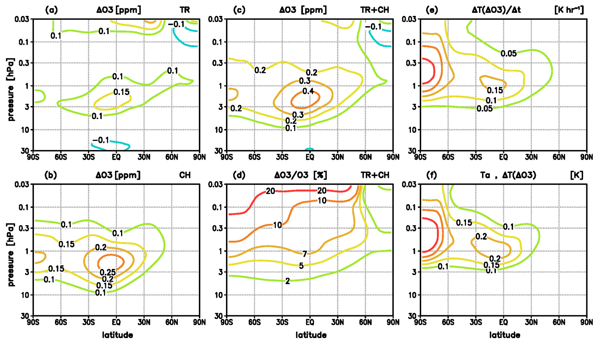
Figure 2 Changes due to ozone–temperature coupling at a specific level induced by an initial GW perturbation with horizontal and vertical wavelengths L_k=500 km and L_m=5 km, and with exponential increase in amplitude with height (initial temperature amplitude T_a(zs)=1 K at zs≈35 km; p=6.28 hPa). (a) Change in ozone due to vertical transport, (b) change in ozone due to photochemistry, (c) total change in ozone, (d) relative change in ozone, (e) change in the heating rate, and (f) change in the temperature perturbation.

For illustration of the induced change in ozone at a specific level (Fig. 2a–d), we assume an initial GW perturbation ${\mathit{\theta }}_{\mathrm{1}}^{\prime }$ with exponentially growing amplitude ${\mathit{\theta }}_a={\mathit{\theta }}_{\mathrm{a}\mathrm{0}}\cdot {\exp }^{(z-zs)/\mathrm{2}H}$, with an initial temperature amplitude T_a0 of 1 K at zs≈35 km (ps=6.28 hPa) increasing to ∼8 K at z≈65 km (p=0.1 hPa). In the present paper, we formulate the solutions for pressure levels p, i.e., the initial perturbation is alternatively described by ${\mathit{\theta }}_a={\mathit{\theta }}_{\mathrm{a}\mathrm{0}}\cdot (ps/p{)}^{\mathrm{1}/\mathrm{2}}$, assuming $p=ps\cdot {\exp }^{(z-zs)/H}$. Introducing the associated perturbation $w_{\mathrm{1}}^{\prime }=-(\partial {\mathit{\theta }}_{\mathrm{0}}/\partial z{)}^{-\mathrm{1}}\cdot d_{\mathrm{0}}{\mathit{\theta }}_{\mathrm{1}}^{\prime }/\mathrm{d}t$ in Eq. (6) leads to $d_{\mathrm{0}}{\mathit{\mu }}_{\mathrm{1}}^{\prime }/\mathrm{d}t=\left[\right(\partial {\mathit{\mu }}_{\mathrm{0}}/\partial z)/(\partial {\mathit{\theta }}_{\mathrm{0}}/\partial z)-b{\mathit{\mu }}_{\mathrm{0}}]\cdot d_{\mathrm{0}}{\mathit{\theta }}_{\mathrm{1}}^{\prime }/\mathrm{d}t$, and, considering $d_{\mathrm{0}}{\mathit{\mu }}_{\mathrm{1}}^{\prime }/\mathrm{d}t=-i{\mathit{\omega }}_{i\mathrm{1}}{\mathit{\mu }}_{\mathrm{1}}^{\prime }$ and $d_{\mathrm{0}}{\mathit{\theta }}_{\mathrm{1}}^{\prime }/\mathrm{d}t=-i{\mathit{\omega }}_{i\mathrm{1}}{\mathit{\theta }}_{\mathrm{1}}^{\prime }$, to an initial ozone perturbation ${\mathit{\mu }}_{\mathrm{1}}^{\prime }={\mathit{\theta }}_{\mathrm{1}}^{\prime }\cdot \left[\right(\partial {\mathit{\mu }}_{\mathrm{0}}/\partial z)/(\partial {\mathit{\theta }}_{\mathrm{0}}/\partial z)-b{\mathit{\mu }}_{\mathrm{0}}$]. For the example of the ascent ($w_{\mathrm{1}}^{\prime }>\mathrm{0}$) shown in Fig. 2, we set ${\mathit{\theta }}_{\mathrm{1}}^{\prime }<\mathrm{0}$, leading to ${\mathit{\mu }}_{\mathrm{1}}^{\prime }>\mathrm{0}$. For L_k=500 km and L_m=5 km, the contributions ${\mathit{\mu }}^{\prime }\left(TR\right)={\mathit{\theta }}_{\mathrm{1}}^{\prime }\cdot \left[\right(\partial {\mathit{\mu }}_{\mathrm{0}}/\partial z)/(\partial {\mathit{\theta }}_{\mathrm{0}}/\partial z\left)\right]$ (related to transport; Fig. 2a) and ${\mathit{\mu }}^{\prime }\left(CH\right)=-b{\mathit{\mu }}_{\mathrm{0}}{\mathit{\theta }}_{\mathrm{1}}^{\prime }$ (related to S^′; Fig. 2b) sum up to a total change of ${\mathit{\mu }}^{\prime }\approx \mathrm{0.2}$ to 0.5 ppm (Fig. 2c) or ${\mathit{\mu }}^{\prime }/{\mathit{\mu }}_{\mathrm{0}}\approx \mathrm{5}$ to 10 % (Fig. 2d) in the USLM region, where the feedback to the heating rate is particularly strong.

The related change in the heating rate at a specific level (Fig. 2e) is given by comparing Eq. (5) with and without ozone–temperature coupling. Assuming that the same initial ascent or adiabatic cooling as above leads to ($w_{\mathrm{2}}^{\prime }-w_{\mathrm{1}}^{\prime }\left)\right(\partial {\mathit{\theta }}_{\mathrm{0}}/\partial z)=Q^{\prime }({\mathit{\mu }}_{\mathrm{1}}^{\prime })$, or, when introducing $w_{\mathrm{2}}^{\prime }=({\mathit{\omega }}_{i\mathrm{1}}/{\mathit{\omega }}_{i\mathrm{2}})\cdot w_{\mathrm{1}}^{\prime }$ to $Q^{\prime }\left({\mathit{\mu }}_{\mathrm{1}}^{\prime }\right)=({\mathit{\omega }}_{i\mathrm{1}}/{\mathit{\omega }}_{i\mathrm{2}}-\mathrm{1})(-{\mathit{\omega }}_{i\mathrm{1}}{\mathit{\theta }}_{\mathrm{1}}^{\prime })=a{\mathit{\omega }}_{i\mathrm{1}}{\mathit{\mu }}_{\mathrm{1}}^{\prime }{\mathit{\mu }}_{\mathrm{0}}^{-\mathrm{1}}$ (where $Q^{\prime }\left({\mathit{\mu }}_{\mathrm{1}}^{\prime }\right)>\mathrm{0}$ in case of $w_{\mathrm{1}}^{\prime }>\mathrm{0}$), Fig. 2e shows that $Q^{\prime }\left({\mathit{\mu }}_{\mathrm{1}}^{\prime }\right)$ reach values of 0.15 K h⁻¹ over the tropics and 0.25 K h⁻¹ at southern summer polar latitudes. Then, consistent with Eq. (16), we yield ${\mathit{\theta }}_{\mathrm{2}}^{\prime }-{\mathit{\theta }}_{\mathrm{1}}^{\prime }=({\mathit{\omega }}_{i\mathrm{1}}/{\mathit{\omega }}_{i\mathrm{2}}-\mathrm{1})\cdot {\mathit{\theta }}_{\mathrm{1}}^{\prime }$ where $({\mathit{\omega }}_{i\mathrm{1}}/{\mathit{\omega }}_{i\mathrm{2}}-\mathrm{1})=-a{\mathit{\mu }}_{\mathrm{0}}^{-\mathrm{1}}\left[\right(\partial {\mathit{\mu }}_{\mathrm{0}}/\partial z)/(\partial {\mathit{\theta }}_{\mathrm{0}}/\partial z)-b{\mathit{\mu }}_{\mathrm{0}}]$ for the change in the potential temperature perturbation, i.e., changes in temperature of 0.2–0.3 K in the USLM region (Fig. 2f). In summary, analogously considering the corresponding change for the descent, we yield an increase in the amplitude of the oscillating GW pattern at a specific level by up to 5 %–10 % in ozone and 0.2–0.3 K in temperature.

For other initial wavelengths (or associated frequencies), the latitude-height dependence is very similar to those shown in Figs. 1d–f and 2, whereas the magnitude of the amplification factor ${\mathit{\omega }}_{i\mathrm{1}}/{\mathit{\omega }}_{i\mathrm{2}}$ becomes smaller in the case of increasing vertical and decreasing horizontal wavelengths, or decreasing frequencies, as illustrated in Fig. 3 for an altitude where ${\mathit{\omega }}_{i\mathrm{1}}/{\mathit{\omega }}_{i\mathrm{2}}$ reach maximum values (1.156 hPa or ≈47 km altitude). Figure 3a shows values of ${\mathit{\omega }}_{i\mathrm{1}}/{\mathit{\omega }}_{i\mathrm{2}}>\mathrm{1.02}$ for wave periods of τ_i>2 h steadily increasing with an increasing initial period up to values between 1.14 and 1.15. This value is limited, on the one side, because of the increasing duration of nighttime with latitude towards equatorial and northern winter regions (denoted by shaded areas), and, on the other side, because of the increasing Coriolis force in southern summer middle and polar regions (i.e., because of ${\mathit{\omega }}_{i\mathrm{1}}^{\mathrm{2}}>f^{\mathrm{2}}$).

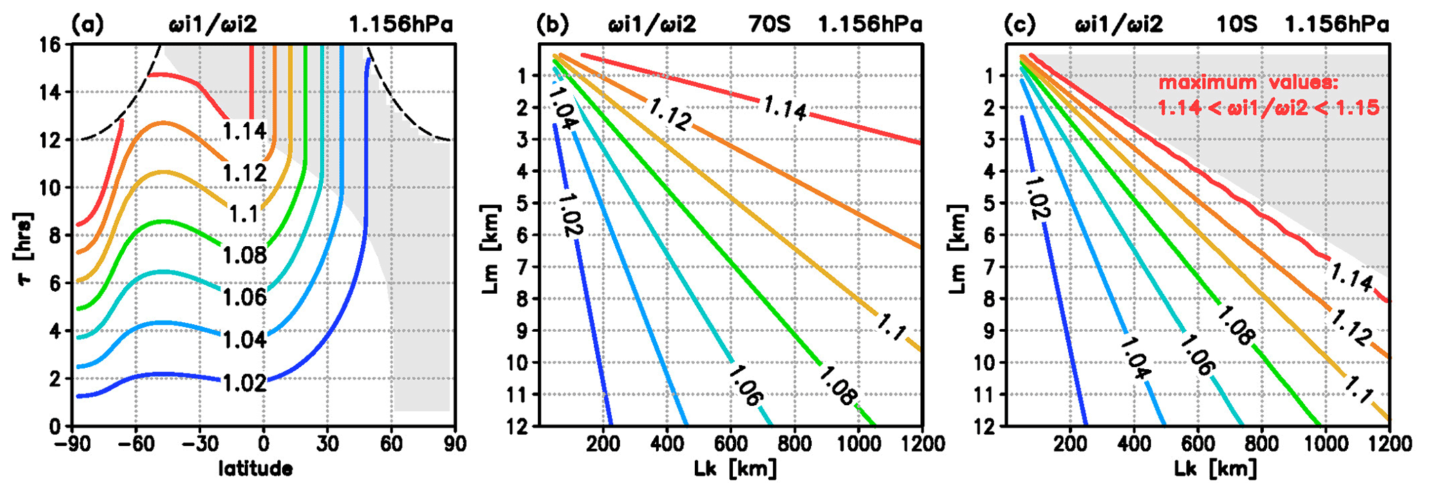
Figure 3 Amplification factor ${\mathit{\omega }}_{i\mathrm{1}}/{\mathit{\omega }}_{i\mathrm{2}}$ at a level of the maximum values of ${\mathit{\omega }}_{i\mathrm{1}}/{\mathit{\omega }}_{i\mathrm{2}}$ (1.156 hPa) illustrating the decrease in the intrinsic frequency with (ω_i2) compared to without (ω_i1) ozone–temperature coupling (compare with Fig. 1e–f), (a) latitudinal distribution of ${\mathit{\omega }}_{i\mathrm{1}}/{\mathit{\omega }}_{i\mathrm{2}}$ as a function of the initial wave period τ_i [in h], and (b–c) dependence of ${\mathit{\omega }}_{i\mathrm{1}}/{\mathit{\omega }}_{i\mathrm{2}}$ on the horizontal and vertical wavelengths L_k and L_m [in km] at (b) 70^∘ S and (c) 10^∘ S. Shaded areas show where the amplification is limited by the length of daytime (τ_i>τ_day).

Consistently, the amplification factor increases with decreasing vertical and increasing horizontal wavelengths (Fig. 3b and c show examples for 70 and 10^∘ S), where the values are limited by the length of daytime in the case of small relations $L_{\mathrm{m}}/L_{\mathrm{k}}$ denoting the conditions where τ_i>τ_day (Fig. 3c, shaded area). Figure 3 also indicates that the examples with L_k=500 km and L_m=5 km (Figs. 1e; 2) and L_k=800 km and L_m=3 km (Fig. 1f) represent scales where ozone–gravity wave interaction is particularly efficient.

Overall, Figs. 1d–f, 2 and 3 illustrate the amplification of GW amplitudes at a specific level and a specific time. As far as the GWs are continuously propagating upward through several levels where ${\mathit{\omega }}_{i\mathrm{1}}/{\mathit{\omega }}_{i\mathrm{2}}-\mathrm{1}>\mathrm{0}$, the amplification will be successively reinforced at each level. This cumulative amplification can lead to much stronger GW amplitudes at upper mesospheric altitudes in the case with ozone–gravity wave interaction than in the case without, as demonstrated in the next subsection.

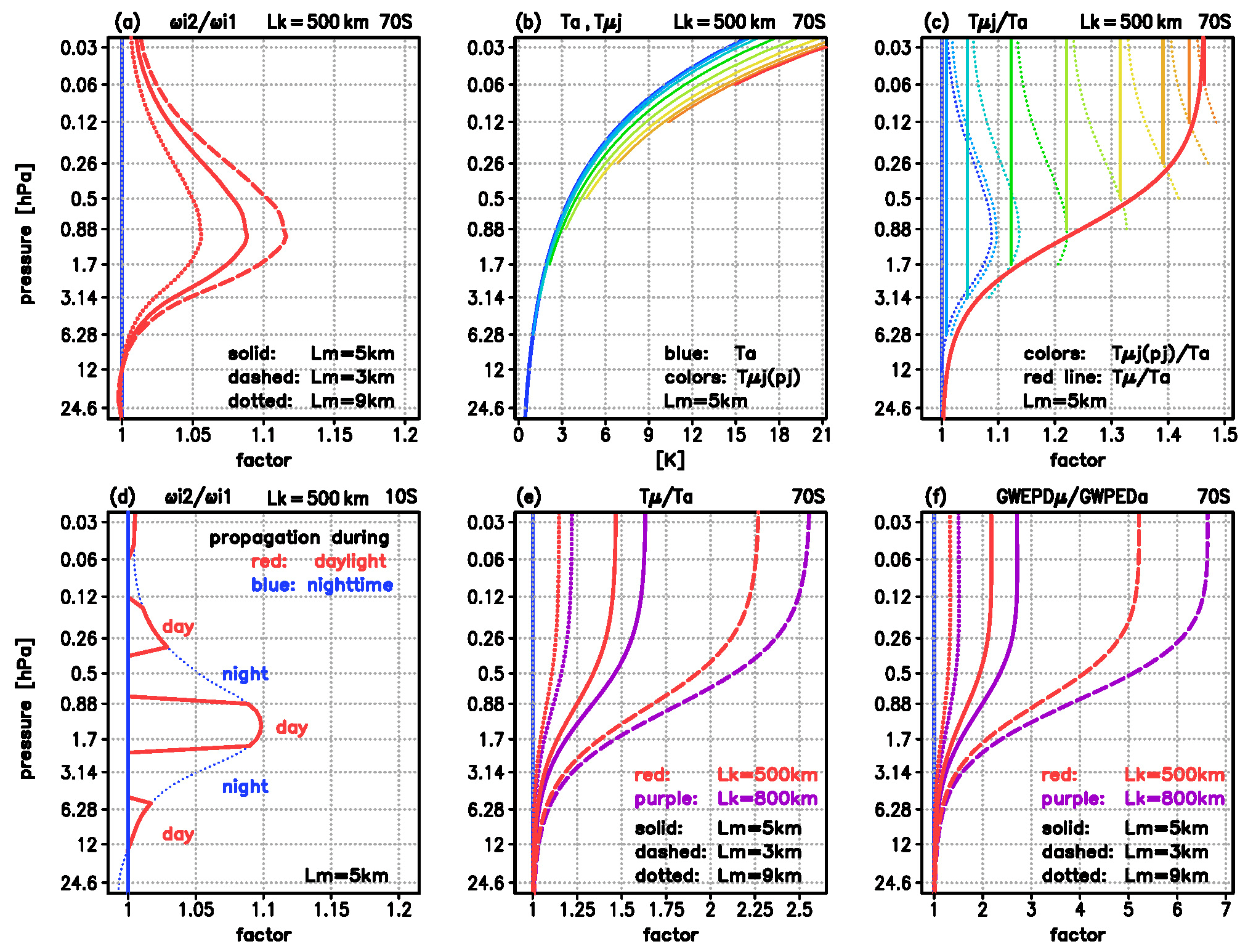
Figure 4 Illustration of the successive amplification of GW amplitudes during the upward level-by-level propagation. (a) Amplification factor ${\mathit{\omega }}_{i\mathrm{1}}/{\mathit{\omega }}_{i\mathrm{2}}$ at 70^∘ S for GW with horizontal wavelength L_k=500 km and vertical wavelength L_m=5 km (solid red line), and, for comparison, L_m=3 (dashed) and L_m=9 km (dotted). (b) Temperature amplitudes for GW with L_k=500 km and L_m=5 km, depicting the initial perturbation T_a (blue) and the successively amplified amplitudes $T_{\mathit{\mu }j}\left(z_j\right){|}_{j=\mathrm{1},n}$ (light blue towards red; here, n=8 for L_m=5 km). (c) Same as (b) but for the relative amplitudes $T_{\mathit{\mu }j}\left(z_j\right){|}_j/T_{\mathrm{a}}$ (solid lines) together with the profiles of the previous level multiplied by ${\mathit{\omega }}_{i\mathrm{1}}/{\mathit{\omega }}_{i\mathrm{2}}$ (i.e., $T_{\mathit{\mu }j-\mathrm{1}}\left(z_{j-\mathrm{1}}\right)\cdot ({\mathit{\omega }}_{i\mathrm{1}}/{\mathit{\omega }}_{i\mathrm{2}})$, dashed lines) and a fitted approach T_μ (thick solid red line, defined by Eq. 18). (d) Same as (a) for the case L_k=500 km and L_m=5 km but at 10^∘ S including the limitation due to the length of nighttime conditions. (e) Relative values $T_{\mathit{\mu }}/T_{\mathrm{a}}$ at 70^∘ S for different horizontal (red: L_k=500 km, purple: L_k=800 km) and vertical (dashed: L_m=3, solid: L_m=5 km, dotted: L_m=9 km) wavelengths. (f) Same as (e) but for the relative values $E_{\mathit{\mu }}/E_{\mathrm{a}}$ of the related gravity wave potential energy density (GWPED, defined by Eq. 19).

2.2 Upward propagating GWs in a background flow

2.2.1 Level-by-level amplification of GW amplitudes

In the following section, a solution for the cumulative amplification during the vertical level-by-level propagation is derived, excluding – to a first guess – other effects like small-scale diffusion, wave-breaking processes, interaction of GWs with atmospheric tides, or so-called secondary GWs. Following the Huygens principle, each point of a propagating wave front at a specific level is the source of a new wave at this level, i.e., a single upward propagating GW, which is amplified at a level z_j−1, is the initial perturbation amplified at the next level z_j. For illustration (Fig. 4a–c), we choose an initial GW with horizontal and vertical wavelengths L_m=500 km and L_m=5 km as above, where the vertical distance between the levels z_j−1 and z_j is set by the initial vertical wavelength Δz=L_m. First, we focus on polar latitudes during southern polar summer (70^∘ S) with daytime conditions only. Thereafter we consider the modification for middle and equatorial latitudes where GWs with weak vertical group velocities propagate through USLM during both daytime and nighttime.

For orientation, Fig. 4a shows the profiles ${\mathit{\omega }}_{i\mathrm{1}}/{\mathit{\omega }}_{i\mathrm{2}}$ for L_k=500 km and L_m=5 km at 70^∘ S (solid), and, for comparison, for L_m=3 (dashed) and L_m=9 km (dotted), indicating the altitude range where ozone–temperature coupling is relevant (note that the depicted distance of pressure levels approximately represents a 5 km distance in altitude). Beginning with a first level at zs≈35 km (6.28 hPa), the wave propagates through eight layers between ≈35 and ≈70 km (0.06 hPa) where the amplification of the amplitude is relevant. At each of these levels, denoted by $z_j=zs+(j-\mathrm{1})\cdot \mathrm{\Delta }z$ (j=1, n; here n=8), the amplitude at z_j will be amplified by the factor ${\mathit{\omega }}_{i\mathrm{1}}\left(z_j\right)/{\mathit{\omega }}_{i\mathrm{2}}\left(z_j\right)$ at z_j. Starting with an exponentially growing amplitude $T_{\mathrm{a}}\left(z\right)=T_{\mathrm{a}}\left(zs\right)\cdot {\exp }^{(z-zs)/\mathrm{2}H}$ (where we set T_a(zs)=1 K again), we yield a new amplitude $T_{\mathrm{a}\mathrm{1}}\left(z_{\mathrm{1}}\right)=T_{\mathrm{a}}\left(z_{\mathrm{1}}\right)\cdot {\mathit{\omega }}_{i\mathrm{1}}\left(z_{\mathrm{1}}\right)/{\mathit{\omega }}_{i\mathrm{2}}\left(z_{\mathrm{1}}\right)$ at the level z₁, defining a new exponentially growing amplitude $T_{\mathit{\mu }\mathrm{1}}\left(z\right)=T_{\mathrm{a}\mathrm{1}}\left(z_{\mathrm{1}}\right)\cdot {\exp }^{(z-z\mathrm{1})/\mathrm{2}H}$. We then yield $T_{\mathrm{a}\mathrm{2}}\left(z_{\mathrm{2}}\right)=T_{\mathit{\mu }\mathrm{1}}\left(z_{\mathrm{2}}\right)\cdot {\mathit{\omega }}_{i\mathrm{1}}\left(z_{\mathrm{2}}\right)/{\mathit{\omega }}_{i\mathrm{2}}\left(z_{\mathrm{2}}\right)$ at the level z₂, defining $T_{\mathit{\mu }\mathrm{2}}\left(z\right)=T_{\mathrm{a}\mathrm{2}}\left(z_{\mathrm{2}}\right)\cdot {\exp }^{(z-z\mathrm{2})/\mathrm{2}H}$, and so forth. Finally, the amplitude at the level z_n in the middle mesosphere is described by

$$\begin{array}{}\text{(17)}& T_{\mathit{\mu }}n\left(z\right)=T_a\left(z\right)\cdot \prod _{j=\mathrm{1}}^n\left[{\displaystyle \frac{{\mathit{\omega }}_{i\mathrm{1}}\left(z_j\right)}{{\mathit{\omega }}_{i\mathrm{2}}\left(z_j\right)}}\right],\end{array}$$

where the product symbol ${\mathrm{\Pi }}_{j=\mathrm{1},n}$ denotes the multiplication with ${\mathit{\omega }}_{i\mathrm{1}}\left(z_j\right)/{\mathit{\omega }}_{i\mathrm{2}}\left(z_j\right)$ at each level $z_{\mathrm{1}}\le z_j\le z_n$. As mentioned above, the solutions are calculated on pressure levels, i.e., z represents the geopotential height, and the vertical distance Δz between the levels is given by $\mathrm{\Delta }z=-({\mathit{\rho }}_{\mathrm{0}}g{)}^{-\mathrm{1}}\mathrm{\Delta }p=-H(T_{\mathrm{0}})\cdot (\mathrm{\Delta }p/p)$, where $H\left(T_{\mathrm{0}}\right)=g/\left(R{T}_{\mathrm{0}}\right)$ is the height-dependent scale height defined by the background. Note that using a constant scale height H₀=7 km instead of H(T₀) only leads to second-order changes in the cumulative amplitude amplification (the sensitivity test is described below in Sect. 2.2.4), because H(T₀) only varies slightly in the USLM region (between ∼7.5 km at summer stratopause altitudes and ∼6.5 km at 70 km).

Figure 4b shows the initial amplitude T_a (blue line) and the series of the successively amplified amplitudes T_μ1, T_μ2, …, T_μn (from light blue towards red line). Figure 4c shows the related series of constant relative values $T_{\mathit{\mu }\mathrm{1}}/T_{\mathrm{a}}$, $T_{\mathit{\mu }\mathrm{2}}/T_{\mathrm{a}}$, …, $T_{\mathit{\mu }n}/T_{\mathrm{a}}$, starting at the level z_j (solid lines) together with the previous values starting at z_j−1, multiplied by the factor ${\mathit{\omega }}_{i\mathrm{1}}/{\mathit{\omega }}_{i\mathrm{2}}$ (dotted lines), illustrating the successively increasing growth of the amplitude during the upward level-by-level propagation. Finally, the amplitudes converge to T_μn(z) when reaching the upper mesosphere, where T_μn(z) is stronger than T_a(z) by a factor of ∼1.47. Figure 4c also shows the fitted relative increase in the amplitude $T_{\mathit{\mu }}/T_{\mathrm{a}}$ (thick red line) describing the continuous change in the growth rate of the amplitude, where T_μ(z), or T_μ(p), is defined by

$$\begin{array}{}\text{(18)}& T_{\mathit{\mu }}\left(p\right)=hs\left(p\right)\cdot T_a\left(p\right)+hm\left(p\right)\cdot T_{\mathit{\mu }}n\left(p\right),\end{array}$$

with weighting functions $hs=p_{\mathrm{0}}^{\mathrm{1.5}}/(p_{\mathrm{0}}^{\mathrm{1.5}}+p_{\mathrm{m}}^{\mathrm{1.5}})$ and $hm=\mathrm{1}-hs$, where p₀ is the background pressure and $p_{\mathrm{m}}\left(\mathrm{70}{}^{\circ }\mathrm{S}\right)\approx \mathrm{0.96}$ hPa the level of the maximum of ${\mathit{\omega }}_{i\mathrm{1}}/{\mathit{\omega }}_{i\mathrm{2}}$ (note that the height of this maximum is slightly decreasing from p_m≈0.89 hPa over the South Pole to p_m≈1.3 hPa over the Equator).

For middle and equatorial latitudes, daytime–nighttime conditions are considered by setting the amplification factor to $F_{\mathrm{d}}={\mathit{\omega }}_{i\mathrm{1}}/{\mathit{\omega }}_{i\mathrm{2}}$ during daytime but to F_d=1 during nighttime over the vertical wave propagation distance of 1 full day. In detail, we define the parameter $L_{\mathrm{day}}=({\mathit{\tau }}_{\mathrm{day}}-\mathrm{0.5}\cdot {\mathit{\tau }}_{\mathrm{0}})/(\mathrm{0.5}\cdot {\mathit{\tau }}_{\mathrm{0}})$, where τ₀=24 h and τ_day is the duration of daytime within 24 h at the latitude ϕ (with L_day=1 during polar summer and L_day=0 at the Equator). Further, considering the vertical group velocity $c_{gz}=\partial {\mathit{\omega }}_{i\mathrm{1}}/\partial m_{\mathrm{1}}=-({\mathit{\omega }}_{i\mathrm{1}}/m_{\mathrm{1}})\cdot ({\mathit{\omega }}_{i\mathrm{1}}^{\mathrm{2}}-f^{\mathrm{2}})/{\mathit{\omega }}_{i\mathrm{1}}^{\mathrm{2}}$ (with initial frequency ω_i1 and vertical wavelength m₁ as a first guess), the sinusoidal wave propagation structure between the middle stratosphere and middle mesosphere is described by $L_{cgz}=\cos (\mathrm{2}\mathit{\pi }{\mathit{\tau }}_{\mathrm{0}}\cdot (z-z_m)/c_{gz})$ changing periodically between 1 and −1 over one wavelength, where z and z_m are given in kilometers and c_gz in kilometers per hour, and where L_cgi=1 at the level p_m, or altitude z_m(p_m). Then, the combined parameter $L_{\mathrm{d}}=L_{\mathrm{day}}+L_{cgi}$ separates the vertical propagation distance into daytime and nighttime fractions by defining a constant value C_d=1 in the case of L_d>1 and C_d=0 in the case of L_d≤1, where the factor $F_{\mathrm{d}}=\mathrm{1}+C_{\mathrm{d}}\cdot \left(\right({\mathit{\omega }}_{i\mathrm{1}}/{\mathit{\omega }}_{i\mathrm{2}})-\mathrm{1})$ provides $F_{\mathrm{d}}={\mathit{\omega }}_{i\mathrm{1}}/{\mathit{\omega }}_{i\mathrm{2}}$ in the case of daytime and F_d=1 in the case of nighttime.

As an example, Fig. 4d shows the profile of the resulting amplification factor F_d at 10^∘ S for a GW with L_k=500 km and L_m=5 km as above, with an associated vertical group velocity c_gz of about 7 km per 12 h, illustrating that we define $F_{\mathrm{d}}\left(z_j\right)={\mathit{\omega }}_{i\mathrm{1}}\left(z_j\right)/{\mathit{\omega }}_{i\mathrm{2}}\left(z_j\right)$, where z_j is located in the daytime region (red) but F_d(z_j)=1, where z_j is located in the nighttime region (blue). The indicated vertical wave propagation distance during daytime increases towards southern summer polar latitudes but decreases towards northern winter polar latitudes. Note that for vertical wavelengths examined in the present paper (L_m≤15 km), a vertical shift of the phase – as defined by the altitude z_m in the definition of L_cgz – does not have a significant impact on the cumulative amplification of the GW amplitudes because of the Gaussian-type structure of the profile of $F_{\mathrm{d}}={\mathit{\omega }}_{i\mathrm{1}}/{\mathit{\omega }}_{i\mathrm{2}}$, which has been verified by several test calculations with levels other than p_m, or altitudes other than z_m.

In the following section, the fitted profiles T_μ are used for further examinations with different horizontal and vertical wavelengths, where the vertical level-by-level amplification is calculated by using the distances Δz=Δz_H of the vertical grid of HAMMONIA instead of Δz=L_m. This includes a smaller amplification factor $F_{\mathit{\omega }}={\mathit{\omega }}_{i\mathrm{1}}/{\mathit{\omega }}_{i\mathrm{2}}$ over the vertical distance Δz_H because of the smaller heating rate perturbation $Q_{\mathrm{\Delta }zH}^{\prime }=(\mathrm{\Delta }{z}_H/L_{\mathrm{m}})\cdot Q^{\prime }$ (see Eq. 11 and the related discussion). However, the resulting differences in the amplification at a specific level over the vertical distance L_m are nearly the same, except for some small differences of less than 0.5 % due to the different vertical resolution (i.e., $F_{\mathit{\omega }}(\mathrm{\Delta }z=L_{\mathrm{m}})\approx \mathrm{1}+\left(F_{\mathit{\omega }}\right(\mathrm{\Delta }z=\mathrm{\Delta }{z}_H)-\mathrm{1})\cdot (L_{\mathrm{m}}/\mathrm{\Delta }{z}_H)$). Additionally, the resulting cumulative amplification in the upper mesosphere remains nearly unchanged ($T_{\mathit{\mu }n}(\mathrm{\Delta }z=L_{\mathrm{m}})\approx T_{\mathit{\mu }nh}(\mathrm{\Delta }z=\mathrm{\Delta }{z}_H)$, where nh is the number of the HAMMONIA levels in the USLM), where small differences between T_μnh and T_μn of less than 10 % occur only at middle and equatorial latitudes in the case of small vertical wavelengths (or small vertical group velocities) when considering the vertical propagation during both daytime and nighttime described below.

2.2.2 Cumulative amplitude amplifications for representative examples

Figure 4e illustrates the dependence of the amplitude amplification on the horizontal and vertical wavelengths L_k and L_m at 70^∘ S, where it is not affected by nighttime conditions. In comparison to the example of L_k=500 km and L_m=5 km leading to a cumulative amplification of ∼1.47 (solid red line), a larger vertical wavelength of L_m=9 km leads to a smaller value of ∼1.15 (dotted red line), but a smaller vertical wavelength of L_m=3 km leads to a larger value of ∼2.27 (dashed red line), because the induced increase in the ozone perturbation μ^′ produces a heating rate perturbation Q^′ within a shorter (in the case of L_m=9 km) or larger (in the case of L_m=3 km) time increment τ_i. For the same reason, the amplification is generally larger if the horizontal wavelength L_k is larger, e.g., in the case of L_k=800 km, the final amplification in the upper mesospheric amplitudes amounts to ∼1.22 for L_m=9 km (dotted purple line), ∼1.63 for L_m=5 km (solid purple line), and ∼2.56 for L_m=3 km (dashed purple line).

The related GWPED (here denoted by E) is derived following Kaifler et al. (2015):

$$\begin{array}{}\text{(19)}& E={\displaystyle \frac{\mathrm{1}}{\mathrm{2}}}{\left({\displaystyle \frac{g}{N}}\right)}^{\mathrm{2}}{\left({\displaystyle \frac{T^{\prime }}{T_{\mathrm{0}}}}\right)}^{\mathrm{2}}.\end{array}$$

Introducing $T^{\prime }=T_{\mathrm{2}}^{\prime }$ and N=N_μ, or $T^{\prime }=T_{\mathrm{1}}^{\prime }$ and N=N₀, leads to the case with (E_μ) or without (E_a) ozone–gravity wave interaction. Figure 4f shows the relative amplitudes $E_{\mathit{\mu }}/E_{\mathrm{a}}$ related to Fig. 4e. In the case of L_k=500 km (red lines), the final amplifications reach values of ∼1.32 for L_m=9 km (dotted), ∼2.17 for L_m=5 km (solid), and ∼5.21 for L_m=3 km (dashed), and in case of L_k=800 km (purple lines) values of ∼1.50 for L_m=9 km (dotted), ∼2.70 for L_m=5 km (solid), and ∼6.62 for L_m=3 km (dashed). Overall, these factors provide a first-order estimate of the effect of ozone–gravity wave coupling at 70^∘ S during polar summer, i.e., in case of large horizontal (≥500 km) and small vertical (≤5 km) wavelengths, we find cumulative amplifications in the upper mesosphere in the order of ∼1.5 to ∼2.5 in the temperature perturbations and in the order of ∼3 to ∼7 in the related GWPED.

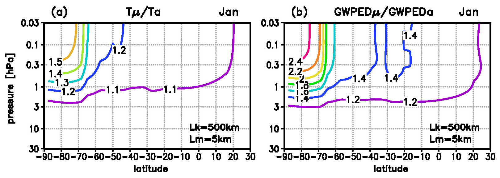
Figure 5 Cumulative amplifications of the GW amplitude during the upward level-by-level propagation for a GW with L_k=500 km and L_m=5 km, (a) Cumulative increase in the temperature amplitudes described by $T_{\mathit{\mu }}/T_{\mathrm{a}}$. (b) Related increase in the gravity wave potential energy density (GWPED) described by $E_{\mathit{\mu }}/E_{\mathrm{a}}$; background conditions: January 2001.

2.2.3 Cumulative amplitude amplifications depending on latitude

For the GW with L_k=500 km and L_m=5 km, Fig. 5 shows the latitudinal dependence of the cumulative amplifications of the temperature perturbation (indicated by $T_{\mathit{\mu }}/T_{\mathrm{a}}$, Fig. 5a) and the related GWPED (indicated by $E_{\mathit{\mu }}/E_{\mathrm{a}}$, Fig. 5b). The values decrease from $T_{\mathit{\mu }}/T_{\mathrm{a}}\approx \mathrm{1.5}$ and $E_{\mathit{\mu }}/E_{\mathrm{a}}\approx \mathrm{2.4}$ over southern summer polar latitudes towards $T_{\mathit{\mu }}/T_{\mathrm{a}}\approx \mathrm{1.2}$ and $E_{\mathit{\mu }}/E_{\mathrm{a}}\approx \mathrm{1.4}$ at lower mid-latitudes (40^∘ S), and then less rapidly towards $T_{\mathit{\mu }}/T_{\mathrm{a}}\approx \mathrm{1.1}$ and $E_{\mathit{\mu }}/E_{\mathrm{a}}\approx \mathrm{1.2}$ at 20^∘ N. Overall, although the amplification of the GW amplitudes decreases rapidly with the decrease in the length of daytime, it is still quite strong at mid-latitudes.

Figure 6 Cumulative amplification of the GW amplitudes similar to that in Fig. 5, but at upper mesospheric levels (0.01 hPa, ∼80 km) for different horizontal and vertical wavelengths L_k (red: 500 km, purple: 800 km) and L_m (dotted: 9 km, solid: 5 km, dashed: 3 km), (a) $T_{\mathit{\mu }}/T_{\mathrm{a}}$, (b) $E_{\mathit{\mu }}/E_{\mathrm{a}}$.

Figure 6 shows the relations $T_{\mathit{\mu }}/T_{\mathrm{a}}$ (Fig. 6a) and $E_{\mathit{\mu }}/E_{\mathrm{a}}$ (Fig. 6b) at upper mesospheric levels (0.01 hPa, ∼80 km) for different horizontal and vertical wavelengths as used for Fig. 4e and f. For both L_k=500 km (red) and L_k=800 km (purple), the amplifications of the temperature perturbations and of the related GWPED are strongest for L_m=3 km (dashed lines), at polar latitudes with values between 2.5 and 3 in $T_{\mathit{\mu }}/T_{\mathrm{a}}$ and between 7 and 9 in $E_{\mathit{\mu }}/E_{\mathrm{a}}$, and at middle and equatorial latitudes between 1.5 and 1.8 in $T_{\mathit{\mu }}/T_{\mathrm{a}}$ and between 2.4 and 3.5 in $E_{\mathit{\mu }}/E_{\mathrm{a}}$. These values decrease with increasing vertical wavelength, i.e., when changing L_m=5 km (solid lines) or L_m=9 km (dotted lines) roughly to ∼1.7 or ∼1.25 in $T_{\mathit{\mu }}/T_{\mathrm{a}}$ and ∼3.0 or ∼1.5 in $E_{\mathit{\mu }}/E_{\mathrm{a}}$ at polar latitudes, and roughly to ∼1.25 or ∼1.2 in $T_{\mathit{\mu }}/T_{\mathrm{a}}$ and ∼1.5 or ∼1.25 in $E_{\mathit{\mu }}/E_{\mathrm{a}}$ at middle and equatorial latitudes. Overall, for the mesoscale GWs with small vertical and large horizontal wavelengths, the cumulative amplifications due to ozone–gravity wave coupling leads to much stronger amplitudes at upper mesospheric altitudes during daytime than during nighttime, in the GW perturbations by a factor between ∼1.5 at summer mid-latitudes and ∼3 for polar daytime conditions, and in the GWPED by a factor between ∼3 at summer mid-latitudes and ∼9 for polar daytime conditions.

Note that vertical momentum flux terms F_GW=ρ₀ ($u^{\prime }{w}^{\prime }$) can be derived from local profiles T^′ if the background is known, i.e., by $F_{\mathrm{GW}}={\mathit{\rho }}_{\mathrm{0}}E\cdot$ (k m⁻¹) (Ern et al., 2004). Therefore, the amplification of the GW amplitudes must lead to the same amplification of the flux term F_GW and, if the GWs do not break at lower levels, of the associated gravity wave drag GWD $=-{\mathit{\rho }}_{\mathrm{0}}^{-\mathrm{1}}\partial F_{\mathrm{GW}}/\partial z$ in the upper mesosphere, suggesting an important effect of ozone–gravity wave interaction on the meridional mass circulation, particularly at polar latitudes. However, more detailed investigations need extensive numerical model simulations with a spectrum of resolved GWs, which is beyond the scope of the present paper.

2.2.4 Sensitivity to varying conditions

In the following section, we estimate the sensitivity of the GW amplitude amplification on nonlinear processes and background conditions which could modulate the first-guess results described above. For example, the decrease in the frequency towards ω_i2<ω_i1 includes a slight decrease in the vertical group velocity towards c_gz2<c_gz1, which can additionally strengthen the process of amplitude amplification because the wave propagates somewhat more slowly through the ULSM region. However, this effect is at least 1 order smaller than the first-order process described above, as derived from test calculations including this effect. For example, for L_k=500 km and L_m=5 km, c_gz2 is smaller than c_gz1 by 15 %–20 % at southern summer polar latitudes and 5 %–10 % at middle and equatorial latitudes. Subsequently, at a specific level, the amplification factor F_d(c_gz2) is stronger than F_d(c_gz1) by 2 %–3 % at polar latitudes and less than 1 % at middle and equatorial latitudes. Including this change in the successive level-by-level propagation leads to a weak successive increase in the cumulative amplifications by ∼5 % at 1 hPa to ∼10 % at 0.01 hPa at polar summer latitudes, and by only ∼1 % at 1 hPa to ∼2 % at 0.01 hPa at middle and equatorial latitudes.

We also estimate the sensitivity of the amplitude amplification on the ozone background μ₀, considering the observed long-term changes in upper stratospheric ozone in the order of up to −8 % per decade (e.g., Sofieva et al., 2017; WMO, 2018), and the uncertainty in the maximum of the heating rate Q₀, which is smaller in the used HAMMONIA data in the order of ∼10 % compared to those derived from satellite measurements, as mentioned above. In the case of a 10 % reduction in ozone, the cumulative amplification in the upper mesospheric GW amplitudes is weaker by about 5 % for the example with L_m=5 km and 10 % for L_m=3 km (i.e., at 70^∘ S, we yield a cumulative amplification of ∼1.4 to ∼2.25 instead of ∼1.5 to ∼2.5), and the related amplification of the GWPED is weaker by about 10 % for L_m=5 km and 20 % for L_m=3 km (at 70^∘ S, a cumulative amplification of ∼2.7 to ∼7.2 instead of ∼3 to ∼9). Analogously, in the case of an increase in Q₀ by 10 %, the cumulative amplification is stronger by 5 % or 10 % in the GW amplitudes and by 10 % or 20 % in the related GWPED amplitudes.

Another question arises about the sensitivity of the effect of ozone–gravity wave coupling to atmospheric tides or the diurnal cycle in stratospheric ozone, which are planetary-scale processes changing the background conditions for the propagation of the mesoscale GW perturbations. For example, Schranz et al. (2018) observed stronger amplitudes in upper stratospheric ozone during daytime than during nighttime in the order of 5 % (summer solstice) to 8 % (May). Such a difference would correspond to a change in the cumulative amplification of the upper mesospheric GW amplitudes or GWPED in the order of 5 % to 10 % or 10 % to 20 %, as follows from the sensitivity of the effect on the prescribed long-term change in stratospheric ozone derived above.

Baumgarten and Stober (2019) derived amplitudes of tides in the order of up to 0.5 K in the middle stratosphere (∼35 km) increasing up to 2 K at ∼50 km and ∼4 K at 70 km, which would correspond to a change in the lapse rate in the order of up to 0.1 K km⁻¹, or in the Brunt-Vaisala frequency $N_{\mathrm{0}}^{\mathrm{2}}$ in the order of 1 %. As follows from Eq. (14), a change in the amplification factor $F_{\mathrm{d}}=N_{\mathrm{0}}^{\mathrm{2}}/N_{\mathit{\mu }}^{\mathrm{2}}$ due to a relative change $\mathrm{\Delta }{N}_{\mathrm{0}}^{\mathrm{2}}/N_{\mathrm{0}}^{\mathrm{2}}$ is given by the factor [$\mathrm{1}+(\mathrm{\Delta }{N}_{\mathrm{0}}^{\mathrm{2}}/N_{\mathrm{0}}^{\mathrm{2}})]/[\mathrm{1}+(\mathrm{\Delta }{N}_{\mathrm{0}}^{\mathrm{2}}/N_{\mathrm{0}}^{\mathrm{2}})(N_{\mathrm{0}}^{\mathrm{2}}/N_{\mathit{\mu }}^{\mathrm{2}})(\mathrm{1}+ab{)}^{-\mathrm{1}}$]. Therefore, for wavelengths L_k≥500 km and L_m≤5 km, a relative increase (decrease) of 1 % in $N_{\mathrm{0}}^{\mathrm{2}}$ would lead to a relative decrease (increase) in the amplification factor of up to 0.035 % at stratopause altitudes, which is much less than the effects of the changes in the vertical group velocity or in ozone described above. Moreover, even if a relative change $\mathrm{\Delta }{N}_{\mathrm{0}}^{\mathrm{2}}/N_{\mathrm{0}}^{\mathrm{2}}$ would be much larger (10 %–50 %), it does not change the amplification factor of a specific level by more than 1 %–3 %, and, hence, the cumulative amplification of the GW amplitudes in the upper mesosphere by more than 5 %–10 %.

Assuming exponential growth of the amplitudes ($\sim e^{(z-zs)/\mathrm{2}H}$) between two levels, the usual approach of a constant scale height (e.g., H∼7 km) instead of a height-dependent scale height $H\left(T_{\mathrm{0}}\right)=g/\left(R{T}_{\mathrm{0}}\right)$ can principally lead to significant differences in the GWPED profiles (e.g., Reichert et al., 2021). For estimating the relevance of a change in H on the cumulative amplitude amplification, the solutions are also calculated for an initial GW perturbation ${\mathit{\theta }}_a={\mathit{\theta }}_{\mathrm{a}\mathrm{0}}\cdot {\exp }^{(z-zs)/\mathrm{2}H}$ with a prescribed scale height H₀=7 km instead of ${\mathit{\theta }}_a={\mathit{\theta }}_{\mathrm{a}\mathrm{0}}\cdot (ps/p{)}^{\mathrm{1}/\mathrm{2}}$, and a related vertical distance $\mathrm{\Delta }z=-H_{\mathrm{0}}\cdot (\mathrm{\Delta }p/p)$ instead of $\mathrm{\Delta }z=-H\left(T_{\mathrm{0}}\right)\cdot (\mathrm{\Delta }p/p)$ (note that H(T₀) varies in the USLM region between ∼7.5 km at summer stratopause altitudes and ∼6.5 km at 70 km). Compared to the values shown in Figs. 5 and 6, the cumulative amplification of the upper mesospheric GW amplitudes is weaker by about 5 % (L_m=5 km) to 10 % (L_m=3 km) over the southern summer polar latitudes and weaker by about 1 % (L_m=5 km) to 3 % (L_m=3 km) at summer mid-latitudes. Correspondingly, the related GWPED values are weaker by about 7.5 % (L_m=5 km) to 20 % (L_m=3 km) over the southern summer polar latitudes, and 1.5 % (L_m=5 km) to 5 % (L_m=3 km) at summer mid-latitudes. Overall, these differences are smaller than the first-order effect of ozone–gravity wave coupling by approximately 1 order, where the use of H(T₀) instead of H₀ at the levels of relevant amplification leads to somewhat stronger amplitude amplifications, particularly over the southern summer polar latitudes, because of the difference between the high background temperatures in the summer stratopause region and the low background temperatures in the summer mesosphere (see Fig. 1a).

2.2.5 Potential effect on mean GW amplitudes

In the following section, the potential effect of ozone–gravity wave interaction is estimated for an average over a representative range of 16 different mesoscale GW events (horizontal wavelengths: 200, 500, 800, and 1100 km, vertical wavelengths: 3, 5, 7, and 9 km; see, for comparison, the amplification factor as function of wavelengths shown in Fig. 3b, c). Although these settings are idealistic, the results provide a first-guess quantification of the potential effect on time–mean GWPED values usually derived from measurements, where several different GWs contribute to the analyzed temperature fluctuations derived from the detected temperature profiles.

Figure 7 Similar to Fig. 6 but for both relative and absolute changes in mean values averaged over 16 representative mesoscale GW events with different horizontal and vertical wavelengths L_k and L_m (L_k: 200, 500, 800, and 1100 km, L_m: 3, 5, 7, and 9 km), (a) relative change in temperature amplitude $T_m/T_{\mathrm{a}}$ (solid red line; dashed lines denote the standard deviation), (b) absolute change T_m−T_a for the case of an initial temperature perturbations T_a0 of 1 K (orange line) and 2 K (purple line) in the middle stratosphere, (c) and (d) same as (a) and (b) but for the GWPED (i.e., for $E_m/E_{\mathrm{a}}$ and E_m−E_a).

Figure 7 illustrates both the relative and absolute changes in the resulting mean upper mesospheric GW temperature amplitudes (Fig. 7a, b) and in the mean GWPED (Fig. 7c, d). The relative increase in the mean temperature amplitude (Fig. 7a, solid red line) is stronger by a factor increasing from about 1.3 (±0.1) at summer low and middle latitudes up to 1.7 (±0.2) at summer polar latitudes (values in brackets denote 1 standard deviation). This corresponds to a stronger increase from about 7 K (±2 K) up to 17.5 K (±4.5 K) in the case of an initial GW perturbation of 1 K in the middle stratosphere (at 6.28 hPa or ≈35 km) (Fig. 7b, solid orange line), and from about 14 K (±4 K) up to 35 K (±9 K) in the case of an initial GW perturbation of 2 K (Fig. 7b, solid purple line).

The relative increase in the mean GWPED (Fig. 7c, solid red line) is stronger by a factor increasing from about 1.7 (±0.2) at summer low and middle latitudes up to 3.4 (±0.8) at summer polar latitudes. This corresponds to a stronger increase in the absolute GWPED values from about 2 J kg⁻¹ (±0.5 J kg⁻¹) at summer low and middle latitudes up to 12 J kg⁻¹ (±3 J kg⁻¹) at summer polar latitudes in the case of an initial GW perturbation of 1 K at 35 km (Fig. 7d, solid orange line), and from about 8 J kg⁻¹ (±2 J kg⁻¹) up to 48 J kg⁻¹ (±0.5 J kg⁻¹) in the case of an initial GW perturbation of 2 K (Fig. 7d, solid purple line).

In summary, we find an absolute increase in the order of 7 to 35 K in the mean GW temperature amplitudes and 2 to 50 J kg⁻¹ in the mean GWPED values, assuming usual initial GW perturbations in the order of 1 to 2 K in the middle stratosphere, where the effect is particularly large during polar daytime conditions. Note that, assuming exponential growth with height only, this potential effect can be much larger in the case of stronger initial amplitudes in the middle stratosphere (the absolute changes in the temperature amplitudes increase linearly and those in the GWPED values quadratically with increasing initial GW perturbations at 35 km) and in specific geographical regions or time periods where primary GWs with large horizontal and small vertical wavelengths are excited (e.g., where L_k≥800 and L_m≤3 km). However, the GWs with very large amplitudes might dissipate by nonlinear wave-breaking processes before reaching the upper mesosphere.

3 Summary and conclusions

The present paper shows that ozone–gravity wave interaction in the upper stratosphere/lower mesosphere (USLM) leads to a stronger increase in gravity wave (GW) amplitudes with height during daytime than during nighttime, particularly during polar summer. The results include information about both the amplification of the GW amplitudes at a specific level and the cumulative increase in the amplitudes during the upward level-by-level propagation of the wave from middle stratosphere to upper mesosphere.

In a first step, standard equations describing upward propagating GWs with and without linearized ozone–gravity wave coupling are formulated, where an initial sinusoidal GW perturbation in the vertical ozone transport and temperature-dependent ozone photochemistry produces a heating rate perturbation as a function of the initial intrinsic frequency, which determines the duration of the perturbation at a specific level over the distance of the initial vertical wavelength. The solution reveals an amplification of the ascending and descending perturbations of the sinusoidal GW pattern at this level, i.e., a decrease in the intrinsic frequency due to both the induced changes in the lapse rate (or Brunt–Vaisala frequency) and the positive feedback of the coupling on the initial GW perturbation, and an associated increase in the GW amplitude by a factor ${\mathit{\omega }}_{i\mathrm{1}}/{\mathit{\omega }}_{i\mathrm{2}}\ge \mathrm{1}$ defined by the relation of the intrinsic frequencies without (ω_i1) and with (ω_i2) ozone–gravity wave coupling. This amplitude amplification is dependent on the horizontal and vertical wavelengths, L_k and L_m, where the effect is most efficient for GWs with L_k≥500 km and L_m≤5 km, or initial frequencies τ_i≥4 h, representing mesoscale GWs forced by cyclones or fronts, or by the orography of mountain ridges like the Rocky Mountains, Andes, or Norwegian Caledonides. For southern summer conditions, strongest amplitude amplifications at specific levels of about 5 %–15 % over the perturbation distance of one vertical wavelength are located near the stratopause, with peak values over the Equator and over summer polar latitudes.

In a second step, an analytic approach of the upward level-by-level propagation of the GW perturbations with and without ozone–gravity wave interaction reveals the cumulative amplitude amplification, where the wave is propagating upward with the vertical group velocity defined by the initial GW parameters, and where daytime–nighttime conditions at middle and equatorial latitudes are considered. Representative examples with different initial wavelengths illustrate that the successive increase in both the GW amplitudes and the related gravity wave potential energy density (GWPED) converge to much stronger amplitudes in the upper mesosphere during daytime than during nighttime. This effect strongly decreases with latitude between summer polar and mid-latitudes because of the decrease in the length of daytime, nearly constant at equatorial latitudes, and decreasing again with latitude towards insignificant values in the winter extratropics.

In summary, the strongest impact of ozone–gravity wave interaction is found for wave periods ≥4 h (related to the wavelengths L_k≥500 km and L_m≤5 km), i.e., in a range of wave periods usually observed at summer middle and polar latitudes. For prescribed single GWs with large horizontal wavelengths (500 to 800 km) and small vertical wavelengths (3 to 5 km), the upper mesospheric GW temperature amplitudes are stronger by a factor between 1.25 and 1.75 at summer low and middle latitudes and between 1.5 and 3 at summer polar latitudes, and the corresponding GWPED by a factor between 1.5 and 3.5 and between 3 and 9. For a representative range of 16 different mesoscale GW events (L_k between 200 and 1100 km, L_m between 3 and 9 km), the mean temperature amplitudes are stronger by a factor between 1.3 at summer low and middle latitudes to 1.7 at summer polar latitudes, e.g., stronger by about 7 to 17.5 K (or 14 to 35 K) in the case of an initial GW perturbation of 1 K (or 2 K) in the middle stratosphere (at ∼35 km). The corresponding relative increase in the mean GWPED is stronger by a factor between 1.7 at summer low and middle latitudes and 3.4 at summer polar latitudes, e.g., for the same example as above, stronger by about 2 to 12 J kg⁻¹ (or 8 to 48 J kg⁻¹). These values range in the order between 2 % and 50 % of the observed order of the mean upper-mesospheric GWPED amplitudes (100 J kg⁻¹). These absolute differences can be larger in the case of stronger initial perturbations in the middle stratosphere, or in specific geographical regions or time periods where primary GWs with large horizontal and small vertical wavelengths (e.g., where L_k≥800 km and L_m≤3 km) are excited. However, the GWs with very large amplitudes might dissipate by nonlinear wave-breaking processes before reaching the upper mesosphere. Overall, these values result from an idealistic approach and cannot entirely explain the details of specific measurements. Nevertheless, they provide a first-guess quantification of the potential effect of ozone–gravity wave interaction on the GW amplitudes.

The variety of horizontal and vertical wavelengths used in the present paper are representative of mesoscale GWs in the USLM region. Observations suggest not only characteristic vertical wavelengths of GWs between ∼2–5 km in the lower stratosphere increasing to ∼10–30 km in the upper mesosphere, but also the existence of large vertical wavelengths greater than 10 km in the ULSM region, particularly above convection in equatorial regions or over southernmost Argentina (e.g., Alexander, 1998; McLandress et al., 2000; Fritts and Alexander, 2003; Alexander and Holton, 2014; Hocke et al., 2016; Baumgarten et al., 2018; Reichert et al., 2021). The results of the present paper suggest that the effect of ozone–gravity wave coupling decreases with increasing vertical wavelengths L_m≥9 km, but strongly increases with decreasing vertical wavelengths L_m≤5 km. The latter could lead to more pronounced GW breaking and dissipation processes in the upper stratosphere during daytime than during nighttime, and – subsequently – to more prominent GWs with larger vertical wavelengths of L_m≥5 km, which would be consistent with the observed GW characteristics at these altitudes presented by Baumgarten et al. (2018).

As mentioned in the introduction, the measurements of Baumgarten et al. (2017) show some evidence that the increase in the GWPED values with height is stronger during full-daytime than during nighttime by a factor of about 2, or, roughly assuming a 2:1 relation of daytime and nighttime (16 h daytime and 8 h nighttime) for high summer mid-latitudes, stronger during daytime than during nighttime by a factor of about 2.5. For comparison, the estimated effect of ozone–temperature coupling for these latitudes (factor of 1.7) is somewhat smaller and would lead to an increase in the nighttime GWPED in the order of ∼50 % (0.7:1.5) of the observed increase. Conclusively, although the difference derived by Baumgarten et al. (2017) might be uncertain as mentioned in the introduction, and although the approach of the present paper cannot entirely explain the details of specific local measurements during a specific time period, the comparison confirms that ozone–gravity wave interaction might be able to produce significant daytime–nighttime differences in the GW amplitudes at high summer mid-latitudes.

Current state-of-the-art general circulation models (GCMs) usually use a variety of prescribed tropospheric sources and tuning parameters in the gravity wave drag (GWD) parameterizations, forcing the middle atmospheric circulation (e.g., McLandress et al., 1998; Fritts and Alexander, 2003; Garcia et al., 2017), where the extreme low temperatures observed in the summer upper mesosphere provide an important benchmark for the quality of the upwelling branch and the associated adiabatic cooling produced by the models. Including ozone–gravity wave interaction into the GCMs might lead to a substantial improvement of the used GWDs and the associated processes driving the summer mesospheric circulation, because the related increase in the GWPED must lead to a similar increase in the vertical momentum flux term determining the GWD. However, the incorporation of ozone–gravity wave interaction into a state-of-the-art GCM using a GWD, or into a numerical model with resolved GWs, needs extensive test simulations, which is beyond the scope of the present paper.

In particular, current GCMs indicate significant changes in the time–mean circulation of the upper mesosphere due to the stratospheric ozone loss over Antarctica during southern spring and early summer via the induced changes in the GWD (Smith et al., 2010; Lossow et al., 2012; Lubi et al., 2016). Long-term changes in upper stratospheric ozone of up to −8 % per decade, derived from satellite measurements (e.g., Sofieva et al., 2017; WMO, 2018), could also affect the mesospheric circulation in the stratosphere and mesosphere by modulating the GW amplitudes and, hence, the GWD. Based on the idealized approach of the present paper, we estimate the sensitivity of the amplification of the GW amplitudes in the upper mesosphere on changes in the ozone background μ₀ and the ozone-related heating rate Q₀(μ₀), revealing that, for horizontal and vertical wavelengths L_k≥500 km and L_m≤5 km, a change of ±10 % in μ₀ or Q₀ results in a change of ±10 % to ±20 % in the upper mesospheric GWPED. Conclusively, the summer mesospheric upwelling might be much more sensitive to the long-term changes in upper stratospheric ozone as has been suggested by the GCMs up to now.

In the approach of the present paper, the variations due to the diurnal cycle in stratospheric ozone and atmospheric tides are excluded to examine the potential effect of ozone–gravity wave interaction as clearly as possible, based on standard equations describing upward propagating GWs in a constant background. On the one hand, these variations can principally modulate the effect of ozone–gravity wave coupling by changing the planetary-scale background conditions for the propagation of the mesoscale GWs. Assuming – to a first order – linear modulations in the background ozone and background lapse rate according to observed diurnal or tidal variations, the sensitivity calculations of the present paper suggest that the related modulations in the amplitude amplification are smaller than the effect of ozone–gravity wave coupling by approximately 1 order. Further test calculations have shown that the use of a height-dependent scale height H(T₀) instead of a constant scale height H₀ at the levels of relevant amplification leads to stronger amplitude amplifications, particularly over the southern summer polar latitudes, because of the high temperatures in the stratopause region and the very low temperatures in the upper mesosphere, where the related differences are also smaller than the first-order process (e.g., in the GWPED, for vertical wavelengths between L_m=5 km and L_m=3 km, between about 7.5 % to 20 % at summer polar latitudes and less than 5 % at summer mid-latitudes).

On the other hand, short-term fluctuations in the balanced zonal and meridional winds due to atmospheric tides can principally lead to changes in the upward GW propagation characteristics, and, hence, to significant daytime–nighttime differences in the growth of the GW amplitudes with height, including nonlinear feedbacks of the propagating mesoscale GWs to the short-term balanced flow components. Further, multistep vertical coupling processes producing secondary GWs in the mesosphere could depend on daytime–nighttime conditions or tidal variations, which could also produce significant daytime–nighttime differences in the growth of the GW amplitudes with height. Considering the remarkably strong effect of ozone–gravity wave coupling suggested by the present paper, we may speculate that it significantly affects these possible changes in the GW amplitudes due to short-term fluctuations in the balanced winds or multistep vertical coupling. However, an unequivocal quantification of the effects of these processes and the involved nonlinear interactions of the daytime–nighttime differences in the GWPED needs much more investigations, e.g., based on extensive GW resolving model simulations with interactive ozone photochemistry, which is beyond the scope of the present paper.

The results of the present paper might stimulate further daytime–nighttime observations of GW activity, particularly at specific measurement sites where the GWs are usually characterized by specific horizontal and vertical wavelengths, e.g., downwind of specific mountain ridges (east of Rocky Mountains, Southern Andes or Norwegian Caledonides), which could be helpful to better understand how ozone–gravity wave coupling is operating in situ.