the Creative Commons Attribution 4.0 License.
the Creative Commons Attribution 4.0 License.
 | 12 Aug 2022
Disentangling the impact of air–sea interaction and boundary layer cloud formation on stable water isotope signals in the warm sector of a Southern Ocean cyclone
Franziska Aemisegger
Stable water isotopes in marine boundary layer water vapour are strongly influenced by the strength of air–sea fluxes. Air–sea fluxes in the extratropics are modulated by the large-scale atmospheric flow, for instance by the advection of warm and moist air masses in the warm sector of extratropical cyclones. A distinct isotopic composition of the water vapour in the latter environment has been observed over the Southern Ocean during the 2016/2017 Antarctic Circumnavigation Expedition (ACE). Most prominently, the secondary isotope variable deuterium excess (d=δ2H–8⋅δ18O) shows negative values in the cyclones’ warm sector. In this study, three mechanisms are proposed and evaluated to explain these observed negative d values. We present three single-process air parcel models, which simulate the evolution of δ2H, δ18O, d and specific humidity in an air parcel induced by decreasing ocean evaporation, dew deposition and upstream cloud formation. Simulations with the isotope-enabled numerical weather prediction model COSMOiso, which have previously been validated using observations from the ACE campaign, are used to (i) validate the air parcel models, (ii) quantify the relevance of the three processes for stable water isotopes in the warm sector of the investigated extratropical cyclone and (iii) study the extent of non-linear interactions between the different processes. This analysis shows that we are able to simulate the evolution of d during the air parcel's transport in a realistic way with the mechanistic approach of using single-process air parcel models. Most importantly, we find that decreasing ocean evaporation and dew deposition lead to the strongest d decrease in near-surface water vapour in the warm sector and that upstream cloud formation plays a minor role. By analysing COSMOiso backward trajectories we show that the persistent low d values observed in the warm sector of extratropical cyclones are not a result of material conservation of low d. Instead, the latter Eulerian feature is sustained by the continuous production of low d values due to air–sea interactions in new air parcels entering the warm sector. These results improve our understanding of the relative importance of air–sea interaction and boundary layer cloud formation on the stable water isotope variability of near-surface marine boundary layer water vapour. To elucidate the role of hydrometeor–vapour interactions for the stable water isotope variability in the upper parts of the marine boundary layer, future studies should focus on high-resolution vertical isotope profiles.
- Article
(7872 KB) - Full-text XML
-
Supplement
(3307 KB) - BibTeX
- EndNote


Extratropical cyclones and their associated fronts are important weather features for moisture cycling over the Southern Ocean (Wernli and Schwierz, 2006; Simmonds et al., 2012; Papritz et al., 2014). Horizontal temperature advection in the cold and warm sector of extratropical cyclones leads to contrasting properties in the two sectors. The cold sector is dominated by equatorward transport of cold and dry air, which leads to intense large-scale ocean evaporation (Bond and Fleagle, 1988; Boutle et al., 2010; Aemisegger and Papritz, 2018) and unstable conditions in the marine boundary layer (MBL, Beare, 2007; Sinclair et al., 2010). In the warm sector, moist and warm air is transported polewards. The conditions in the warm sector are close to saturation, which can lead to weak or even negative surface heat fluxes and generally a stable MBL (Beare, 2007; Sinclair et al., 2010). These contrasting conditions in the cold and warm sector are also reflected in the MBL water vapour's isotopic composition, which is a powerful tracer of moist atmospheric processes. The concentration of stable water isotopologues (SWIs) of water vapour is altered during phase changes due to so-called isotopic fractionation, and, thus, a distinct isotopic signal is imprinted in the water vapour by the moist diabatic processes that occur along its transport pathway. Understanding the formation of SWI anomalies in the cold and warm sector of extratropical cyclones, thus, gives important insight into the dominant processes affecting the moisture budget of air parcels associated with extratropical cyclones.
The abundance of SWIs is given by the δ notation, which is defined by the relative deviation of the isotopic ratio of the sample from an internationally accepted standard ratio representing the ocean water isotope composition: and . Rsample is the isotopic ratio of the sampled water vapour, defined as the ratio between the minor (heavy) and the major (light) isotope. and define the isotopic composition of the Vienna Standard Mean Ocean Water (VSMOW2). The strength of isotopic fractionation depends on environmental conditions. Ambient temperature is the main factor affecting equilibrium fractionation that occurs due to the different, temperature-dependent saturation vapour pressure of SWIs. Non-equilibrium fractionation, a second kind of isotopic fractionation, occurs in non-equilibrium conditions, additionally to equilibrium fractionation, in the presence of humidity gradients due to differences in the molecular diffusion velocity of the water isotopologues. For example, humid air that is supersaturated with respect to the sea surface temperature (SST) can experience dew deposition on the ocean surface, which is accompanied by non-equilibrium fractionation due to the humidity gradient towards the ocean surface (Thurnherr et al., 2021). Dew deposition and the non-equilibrium fractionation effects accompanying it have been extensively studied over land as a water input into different ecosystems (e.g. Wen et al., 2012; Li et al., 2021). The secondary isotope variable deuterium excess (d=δ2H–8⋅δ18O) is a measure of non-equilibrium fractionation and therefore a tracer of diffusion processes involved in ocean evaporation and dew deposition.
In the extratropics, the SWI abundance in MBL water vapour is shaped by various processes that are related to extratropical cyclones. The strongest short-term SWI variations are observed during frontal passages. The passage of a cold front leads to a decrease in δ values (Gedzelman and Lawrence, 1990), which is caused by below-cloud processes, such as rain evaporation, equilibration of rain and water vapour, and by the horizontal advection of air masses with low δ values behind the cold front (Pfahl et al., 2012; Aemisegger et al., 2015; Graf et al., 2019). Fewer studies are available on the isotopic variability in water vapour during warm front passages. Gedzelman and Lawrence (1990) showed that δ18O increases across the warm front due to the advection of isotopically enriched air masses in the warm sector. These strong changes in SWIs across fronts reflect, on the one hand, the precipitation-related processes along the fronts and, on the other hand, the contrasting properties and origin of water vapour in the cold and warm sector of extratropical cyclones, respectively, with typically high δ values in the warm sector and low δ values in the cold sector (Dütsch et al., 2016; Thurnherr et al., 2021).
Moisture transport over the Southern Ocean can occur over long distances. Precipitation in Antarctica can originate from sub-tropical regions due to the suppression of ocean evaporation in the warm sector of extratropical cyclones (Terpstra et al., 2021). During this long-range transport, d can change due to non-equilibrium processes or changes in the ambient temperature that impact the ratio of the equilibrium fractionation factors of 1HO and 1H2HO (Dütsch et al., 2019; Appendix A in Thurnherr et al., 2021). A detailed understanding of processes that influence d during transport in the warm sector is therefore needed. Low or negative d has been observed in near-surface water vapour in the warm sector of Southern Ocean cyclones (Thurnherr et al., 2021), which is in contrast to high d observed in the cold sector of extratropical cyclones due to strong ocean evaporation (Gat et al., 2003; Uemura et al., 2008; Aemisegger and Sjolte, 2018). Vertical airborne SWI profiles showed that negative d can be seen also close to the boundary layer top and has been associated with the evaporation of cloud and rain droplets (Sodemann et al., 2017; Salmon et al., 2019). For near-surface water vapour, three processes have been identified based on a statistical analysis, which can lead to low d in the warm sector of extratropical cyclones: dew deposition on the ocean surface, decreasing ocean evaporation and cloud formation as a result of a moist-adiabatic ascent (Thurnherr et al., 2021). In this study, we investigate the role of these three processes in a quantitative way, for a selected Southern Ocean cyclone. A mechanistic approach is used to better understand the lifetime and characteristics of low d in near-surface water vapour of the warm sector.
In situ measurements of SWIs are limited in time and space. Therefore, modelling approaches of various complexity have been often used to analyse the large-scale setting and to identify the underlying processes driving the measured SWI signals' variability. Isotope-enabled numerical weather and climate models (e.g. Joussaume et al., 1984; Blossey et al., 2010; Werner et al., 2011; Pfahl et al., 2012; Eckstein et al., 2018) allow for detailed studies of the evolution of SWIs during transport (Dütsch et al., 2018; Dahinden et al., 2021). In addition to these complex numerical models, single-process models allow us to investigate the factors controlling specific processes and their effect on the isotopic composition of water vapour. Different approaches have been used to model the isotopic composition of MBL water vapour, of which many involve the Craig and Gordon (1965) model (denoted CG65 hereafter). The CG65 model is a process model simulating the isotopic composition of water vapour that evaporates from a water reservoir. The comparison of measured SWIs in the MBL water vapour with the simulated isotopic composition of evaporated water vapour using the CG65 model has proven useful to estimate the contribution of ocean evaporation to the MBL water vapour (Benetti et al., 2014). Benetti et al. (2018) showed that the isotopic composition of water vapour in the subtropical MBL is a result of mixing of water vapour from ocean evaporation with dry air from the free troposphere using a linear mixing model combined with the CG65 model. Adopting a Lagrangian point of view, Pfahl and Wernli (2009) followed air parcel trajectories experiencing ocean evaporation over the Mediterranean and modelled the isotopic composition of the water vapour using the CG65 model. Such an air parcel model (APM) allows us to simulate the temporal evolution of SWIs in water vapour during the transport of an air parcel due to specific processes. In principle, APMs can also be designed for other processes such as dew deposition or cloud formation. In this study, we develop three single-process APMs to simulate processes influencing SWIs in the warm sector. We confront the results from these APMs with measurement and a simulation with a SWI-equipped regional weather prediction model to understand the relative importance of ocean evaporation, dew deposition and cloud formation for the isotopic composition of near-surface water vapour in the warm sector of an extratropical cyclone.
This study is structured in the following way: in Sect. 2, the data sets used are described. The single-process APMs are introduced in Sect. 3 and applied in a case study of a Southern Ocean cyclone in Sect. 4. Section 5 presents the conclusions of this study.
This study is based on measurements of SWIs in water vapour, as well as meteorological variables from the Antarctic Circumnavigation Expedition (ACE), and on a simulation using the isotope-enabled regional numerical weather prediction model COSMOiso (Pfahl et al., 2012). These two data sets are briefly introduced in the following.
2.1 Ship measurement
ACE took place from 21 December 2016 to 19 March 2017 in the Southern Ocean, and a variety of meteorological data are available from this expedition (Schmale et al., 2019). In this study, we use the laser spectrometric measurements of SWIs in water vapour and specific humidity (qa) at 13.5 m a.s.l. (Thurnherr et al., 2020a), merged SST from in situ measurements and satellite products (Haumann et al., 2020), air temperature (Ta) and air pressure (pa) from the onboard weather station (Landwehr et al., 2019), and rainfall rates along the ship track from continuous micro rain radar measurements (Gehring et al., 2020). For the isotope measurements a Picarro cavity ring-down laser spectrometer was used. The instrument and measurements are characterised in detail in previous studies (Aemisegger et al., 2012; Thurnherr et al., 2020a). The relative humidity with respect to sea surface temperature is calculated using the measured qa, SST and pa, where qs is the saturation specific humidity. All measurement data are used at an hourly time resolution.
2.2 Regional numerical model simulation and air parcel trajectories
In this study, SWI signals in the warm sector of an extratropical cyclone will be investigated in a case study using 1-hourly fields from a COSMOiso simulation in the southern Indian Ocean. The limited-area model COSMOiso (Pfahl et al., 2012) is an isotope-enabled version of the non-hydrostatic numerical weather and climate prediction model COSMO (Steppeler et al., 2003). The 1-month, nudged COSMOiso simulation was performed for the time period 13 December 2016 to 12 January 2017 with a horizontal grid spacing of 0.125∘, corresponding to ∼ 14 km, 40 vertical levels and treating deep convection explicitly (shallow and deep convection parameterisations were switched off). The choice of treating convection explicitly at the resolution of the model grid is motivated by insights from recent studies (e.g. Vergara-Temprado et al., 2020), which show that convection parameterisation schemes can be switched off at coarser resolutions than previously thought (e.g. on the order of 10 km). Such a setup with explicit convection has been evaluated carefully by comparing it to COSMOiso simulations with parameterised convection and isotope observations from multiple platforms in previous studies (Dahinden et al., 2021; de Vries et al., 2021). The chosen grid spacing of 14 km allows for a large domain spanning an area of that is centred at 47∘ S, 18∘ E (Fig. 1a) and within which the regional model can develop its own isotope meteorology at the mesoscale, which is independent of the global model driving the COSMOiso simulation at the boundaries. Six-hourly fields of the global ECHAM5-wiso model (Werner et al., 2011) are used as initial and boundary data. Horizontal winds above 850 hPa are spectrally nudged to the ECHAM5-wiso wind field during the COSMOiso simulation. A detailed description and validation of the simulation was done by Thurnherr et al. (2021).

Figure 1(a) Mean SST during the COSMOiso simulation; the model domain is shown by the thick black line, and the selected subregion in panel (b) is shown with a red rectangle in panel (a). (b) Simulated d on the lowest model level (filled contours) and sea level pressure at 22:00 UTC on 26 December 2016 (grey contours, every 5 hPa). Additionally, important regions for the case study are highlighted: the warm sector (yellow line), the region of low d behind the warm front (solid black line, region WF) and ahead of the cold front (dashed black line, region CF), and the ACE track (white dashed line; white diamond for the ship position at 22:00 UTC on 26 December 2016).
Using the COSMOiso three-dimensional wind fields, 4 d backward and 2 d forward trajectories are calculated using the Lagrangian analysis tool LAGRANTO (Wernli and Davies, 1997; Sprenger and Wernli, 2015). The trajectories are started at 22:00 UTC on 26 December 2016 from the warm sector of an extratropical cyclone, more specifically from a region with warm temperature advection (Ta-SST > 1 ∘C) and negative d on the lowest model level (regions CF and WF in Fig. 1b; for details see Sect. 4.2), from every fifth model grid point (i.e. approximately every 70 km), and at heights between 10 and 50 m a.s.l. in 10 m steps. This leads to a total of 2582 trajectories. Several variables are interpolated along the trajectories to analyse the SWI evolution during transport.
To quantify the effect of different processes on the SWI signals in the MBL, in particular on observed values of negative d in water vapour in a cyclone's warm sector, single-process models are developed and applied in this study. These models represent the SWI evolution in an air parcel due to three processes separately, which, as discussed in the introduction, are potentially involved in the formation of negative d in the warm sector of cyclones: the air parcel model APMevap simulates ocean evaporation, APMdew simulates dew deposition on the ocean surface during advection over an SST gradient and APMray simulates cloud formation during a moist-adiabatic ascent.
We illustrate the setup and behaviour of the three air parcel models with exemplary simulations in typical environments for air parcels arriving in the warm sector of an extratropical cyclone. Before describing the model setup and the simulations in more detail below, we first show and qualitatively compare the three APMs in terms of the simulated behaviour in the q–δ and q–d phase spaces, which are frequently used in the literature (e.g. Noone et al., 2011; Benetti et al., 2018). In a da–δ18Oa phase space (Fig. 2a), each model shows a specific evolution during the simulation. All three APMs show a decrease in da during the first part of the simulations, yet with a different behaviour with respect to δ18Oa and qa. δ18Oa increases in the APMdew and APMevap simulations, while it decreases continuously in the APMray simulation. This leads to a negative d–δ18Oa slope for APMdew and APMevap and a positive slope for APMray at the beginning of the simulation. The decrease in da for APMevap can be distinguished from the da decrease simulated by APMdew and APMray in the da–qa phase space. While qa decreases in the APMray and APMdew simulations, qa increases in the APMevap simulation. Therefore, each APM has a unique signature, when combining the da–δ18Oa and the da–qa phase spaces. These different signatures will be used in Sect. 4.3 to disentangle the importance of these different moist processes along COSMOiso trajectories in the warm sector of a Southern Ocean cyclone.
The single-process models are constrained by a prescribed SST gradient and the moist-adiabatic ascent (Rayleigh fractionation) along their path. The change in the isotopic composition of the air parcel is expressed explicitly as a function of qa and implicitly as a function of time, due to changes in qa with time related to surface fluxes or condensation in clouds. In all three models, and in accordance with the COSMOiso simulation, the formulation by Horita and Wesolowski (1994) is used for the equilibrium fractionation factors and a wind-speed-independent formulation by Pfahl and Wernli (2009) for the non-equilibrium fractionation factors. For the isotopic composition of the ocean we use ECHAM5-wiso ocean surface isotope data (Werner et al., 2011), which is based on an observational data set for δ18O (LeGrande and Schmidt, 2006). The δ2H of sea surface water is assumed to follow the relation of global meteoric waters (Craig and Gordon, 1965) and is thus equal to δ18O multiplied by a factor of 8. This setting leads to ocean surface water isotope values in the study region of δ18O ≃0.2 ‰, δ2H ‰ and d ≃ 0 ‰.

Figure 2Phase space diagrams of (a) d versus δ18O and (b) d versus qa for the example simulations with APMevap (![]() ), APMdew (+) and APMray (∘) discussed in Sect. 3.1, 3.2 and 3.3. The lines are coloured from the start to the end position. The black arrows show the direction from the start to the end during the simulation.
), APMdew (+) and APMray (∘) discussed in Sect. 3.1, 3.2 and 3.3. The lines are coloured from the start to the end position. The black arrows show the direction from the start to the end during the simulation.
The evolution of the isotopic composition of water vapour in APMdew, APMevap, and APMray and its dependence on the model setup are discussed in detail for each model in the following.
3.1 Moisture uptake by ocean evaporation during advection over an SST gradient
Ship-based measurements of SWIs in water vapour are strongly influenced by ocean evaporation. Air exposed to intense ocean evaporation can be identified by high d in water vapour (e.g. Pfahl and Wernli, 2008; Aemisegger and Sjolte, 2018; Thurnherr et al., 2021) and in downstream precipitation (Aemisegger, 2018). The strength of ocean evaporation depends primarily on the relative humidity with respect to sea surface temperature, hs, and the wind speed. The lower hs is, the stronger the ocean evaporation flux is and the stronger the non-equilibrium fractionation effect becomes. For an air parcel experiencing continuous moistening due to ocean evaporation, hs increases if entrainment of drier air from above is neglected. This leads to a decrease in the ocean evaporation flux and thus a decrease in the strength of non-equilibrium fractionation. A further factor influencing hs is SST, which, over a spatial SST gradient, influences the saturation specific humidity qs. Due to the meridional flow in the cold and warm sectors of extratropical cyclones, advection in these cyclone-relative regions typically leads to a change in SST seen by the air parcel during transport, which thus implies a change in hs. The evolution of the isotopic composition of an air parcel, which is continuously moistened by ocean evaporation, while it crosses an SST gradient from the warmer to the cooler side is simulated with a single-process air parcel model.
3.1.1 APMevap setup
Here, we are interested in the SWI evolution along a trajectory in the warm sector moving poleward over the Southern Ocean, over a negative SST gradient during which d is expected to decrease. To simulate the air parcel's movement over an SST gradient, a linear decrease in SST from an initial SST0 to a final SSTend is predefined in this model. The SST along the trajectories defines the evolution of qs during the simulation. The initial specific humidity qa of the air parcel is prescribed such that the initial hs<1.0. During the simulation, qa is increased stepwise by an amount Δqa, which is proportional to the evaporation flux E, which in turn is proportional to (qs−qa), assuming that turbulent mixing is constant. Thus, any mixing with moisture around the parcel is neglected except for the input from ocean evaporation. The evolution of the isotopic composition of the air parcel is calculated iteratively by linear mixing of the air parcel's humidity with the freshly evaporated moisture Δqa. This gives the isotopic ratio of the water vapour in the air parcel at step i+1:
where Ra,i is the isotopic ratio of the water vapour in the air parcel at step i and . This stepwise increase in q continues until qa≈qs, which corresponds to saturated conditions. The isotopic ratio of the evaporation flux Rflux is calculated using the model by Craig and Gordon (1965), with the isotopic ratio of evaporated water vapour defined as
where Roc is the isotopic ratio of the ocean surface water. αe<1 is the equilibrium fractionation factor, and αk≤1 is the non-equilibrium fractionation factor of vapour with respect to liquid. In this air parcel model, the effects of evaporative cooling on the SST and evaporative enrichment on Roc are neglected.
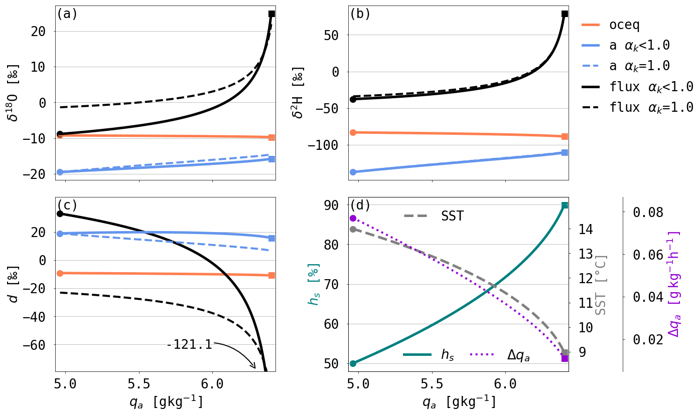
Figure 3Evolution of (a) δ18O, (b) δ2H and (c) d as a function of the air parcel's specific humidity qa in an example simulation with APMevap (see text for details). The blue line shows the isotopic composition of the water vapour in the air parcel (a), the orange line shows that of the equilibrium vapour with the ocean surface (oceq) and the black line shows that of the evaporation flux (flux). For dflux, the end composition is not shown but indicated by −121.1 ‰ in panel (c). Panel (d) shows the SST (grey dashed line), hs (green solid line) and Δqa (violet dotted line) during the simulation. The values of Δqa are calculated assuming that the SST decrease occurred over 36 h. The simulation is shown with non-equilibrium fractionation (αk<1.0, solid lines in panels a–c) and without (αk=1.0, dashed lines in panels a–c). The dots denote the start and the squares the end of the simulation.
3.1.2 An example simulation of APMevap
For an exemplary APMevap simulation, the SST gradient is defined by SST0=14 ∘C and a linear decrease of 0.14 ∘C h−1, which represents the SST evolution expected along a trajectory moving polewards at a speed of 30 km h−1 in the warm sector of an extratropical cyclone (see Supplement Fig. S1c). The simulation is initialised with g kg−1 (and, thus, hs=0.5 because qs=10.0 g kg−1 at 14 ∘C), (qs−qa), δ2H137 ‰, and δ18O19.5 ‰, and the results are shown in Fig. 3. The initial values are chosen based on conditions observed during periods with ocean evaporation along the trajectories arriving in the warm sector of the discussed Southern Ocean cyclone in our COSMOiso simulation. We relate the uptake increment Δqa to the vertical gradient in qa following the formulation of the bulk surface evaporation flux parameterisation, while neglecting the effect of wind speed and using a constant proportionality factor . This proportionality factor determines the SST gradient perceived by the air parcel and sets the time until saturation in the air parcel is reached. The simulation was stopped when hs=90 % because ocean evaporation gets very weak close to saturation. Next to the isotopic composition of the water vapour and the evaporation flux, the equilibrium vapour from the ocean surface water is shown in Fig. 3 (orange line), which represents the isotopic composition that the water vapour would have if it was in thermodynamic equilibrium with the ocean surface. The equilibrium vapour composition is equal to and changes slightly during the simulation due to changes in SST. During the simulation, δ18Oa and δ2Ha in the vapour phase increase towards δ18Ooceq and δ2Hoceq, respectively (Fig. 3a, b). da decreases continuously from its initial value of 19.0 ‰ to 15.8 ‰ at hs=90 % (Fig. 3c). This SWI evolution is the result of the equilibration of the water vapour with the ocean surface, which leads to a general increase in δ values and decrease in d during the simulation, and the effect of non-equilibrium fractionation, which mostly influences the SWI evolution at low hs. The effect of non-equilibrium fractionation on the SWI evolution during the simulation can be quantified by comparing the simulation with non-equilibrium fractionation (αk<1.0) to a simulation with pure equilibrium fractionation (αk=1.0). δ18Oflux and δ2Hflux show lower values in the simulation with non-equilibrium fractionation than during pure equilibrium fractionation, because of the lower diffusion velocity of heavy water molecules compared to the light water molecule. Due to the strong non-equilibrium fractionation, d stays at relatively high values in the beginning of the simulation with αk<1.0. As hs increases and the effect of non-equilibrium fractionation weakens, δ18Oa and δ2Ha increase further and d decreases. The decrease in SST during the simulation leads to a faster saturation of the air parcel and weaker non-equilibrium fractionation than in the simulation without SST changes (not shown). Therefore, the advection over a negative SST gradient accelerates the da decrease.
The example simulation with APMevap shows that continuous ocean evaporation into an air parcel, which is moving over a negative SST gradient, leads to a decrease in da and an increase in δ18Oa and δ2Ha. The detailed evolution of the water vapour isotope signals depends on the strength of non-equilibrium fractionation, which is as a function of hs and SST. In Sect. 4, the evolution of SWIs in a simulation with APMevap will be compared to the evolution along COSMOiso backward trajectories, which arrive in the warm sector of an extratropical cyclone and experience ocean evaporation over decreasing SST during several days before arrival.
The example APMevap simulation discussed here was stopped at hs=90 %. If the simulation was not stopped, hs would eventually exceed 100 % if the SST continued to decrease, and, thus, the air parcel would become supersaturated with respect to the SST. The effect of supersaturated conditions on the SWI composition of water vapour in the air parcel is discussed in the next section with the dew deposition APM.
3.2 Moisture loss by dew deposition on the ocean surface during advection over an SST gradient
Measurements of SWIs during ACE showed low or negative da in combination with high δ2Ha and δ18Oa during periods of warm temperature advection, i.e. Ta − SST > 1 ∘C and positive anomalies in qa (Thurnherr et al., 2021). In these situations, the atmosphere is often supersaturated with respect to the SST such that dew deposition occurs on the ocean surface. To model the corresponding evolution of the SWI composition of the atmospheric water vapour in a supersaturated air parcel moving over a negative SST gradient and arriving in the warm sector of an extratropical cyclone, an approach similar to APMevap is chosen. In the following, the model setup of the dew deposition air parcel model is described, and the SWI evolution during an exemplary simulation is shown and discussed.
3.2.1 APMdew setup
The APMdew describes the evolution of qa and SWIs in an air parcel, which experiences continuous dew deposition while moving over an SST gradient. A linear decrease in SST during the simulation is assumed to represent the poleward movement of the air parcel over the Southern Ocean in the same way as in APMevap. In contrast to APMevap, there is only a moderate decrease in SST in APMdew based on the SST gradient along trajectories experiencing dew deposition in the COSMOiso domain of this study (0.075 ∘C h−1).
We initiate an air parcel with a specific humidity and, thus, a supersaturation of . The air parcel then equilibrates with the ocean surface during the simulation by iteratively decreasing qa in the air parcel by an amount Δqa, which is proportional to (qa−qs), equivalent to the approach in APMevap. The isotopic composition of the water vapour can be iteratively calculated, which leads to the following expression of Ra at simulation step i+1:
Rflux is equivalent to the composition of the evaporation flux given by Craig and Gordon (1965) (Eq. 2) as isotopic fractionation during dew deposition can be described by the same bulk aerodynamic formulation as ocean evaporation (see Appendix A1).
Furthermore, it is assumed that the Roc is not altered by the small amount of deposited dew and that temperature variations due to equilibration or phase changes can be neglected. In the following, a simulation of the APMdew is described in detail to highlight the key factors influencing the SWI evolution during dew deposition.
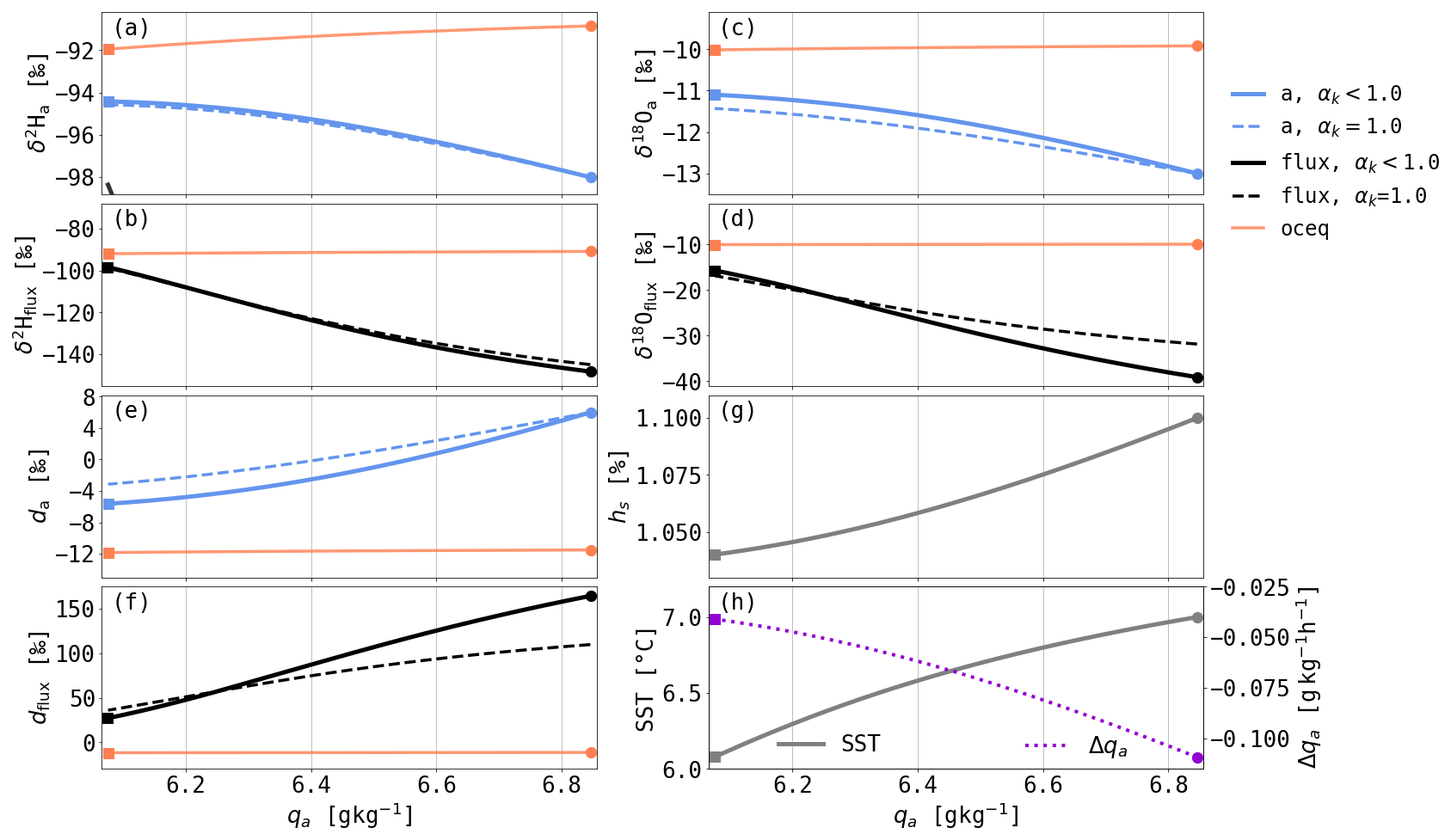
Figure 4Evolution of (a, b) δ2H, (c, d) δ18O and (e, f) d as a function of the air parcel's specific humidity qa in an example simulation with APMdew (see text for details). The blue line shows the isotopic composition of the water vapour in the air parcel (a), the orange line shows that of the equilibrium vapour with the ocean surface (oceq) and the black line shows that of the dew deposition flux (flux). The simulation is shown with non-equilibrium fractionation (αk<1.0, solid lines in panels a–f) and without (αk=1.0, dashed lines in panels a–f). Furthermore, the evolution of (g) hs and (h) the SST (grey solid line) and Δqa (purple dashed line) during the simulations is shown. The values of Δqa are calculated assuming that the SST decrease of 0.9 ∘C occurred over 12 h. Notice that the simulations start to the right (dots) and end to the left (squares) as the air parcel loses moisture during dew deposition.
3.2.2 An example simulation with APMdew
Figure 4 shows the evolution of the isotopic composition of the water vapour and the dew deposition flux as a function of qa for a simulation using the APMdew. During the simulation, SST decreases from 7 ∘C (thus g kg−1) to 6.1 ∘C. These values are chosen to represent typical environmental conditions for an air parcel experiencing dew deposition for 12 h in the warm sector of an extratropical cyclone (see Supplement Fig. S1). The simulation is initialised with hs=1.1, which means that g kg−1. Further, we set (qs−qa), δ2Ha,0 = −98 ‰ and δ18Oa,0 = −13 ‰. The simulation is stopped if hs decreases below 1.04 because the moisture fluxes become very small close to equilibrium conditions. As for APMevap, we chose the initialisation according to typical conditions observed during periods with dew deposition along the trajectories arriving in the warm sector of the discussed Southern Ocean cyclone in our COSMOiso simulation.
The APMdew simulation shows a decrease in da while δ18Oa and δ2Ha increase toward δ18Ooceq and δ2Hoceq, respectively. The decrease in da of 11.6 ‰ is in a similar range as the decrease in da during the example simulation with APMevap (Fig. 3). Non-equilibrium fractionation has an opposite effect on the changes in δ18Oa, δ2Ha and da in APMdew compared to APMevap, because of the opposite direction of the moisture flux that is here from the atmosphere to the ocean.
The specific evolution during the simulations depends on the one hand on the initial isotopic composition of the air parcel, which affects the rate of change in δ values during the simulation due to its control on the ocean–atmosphere isotopic gradient. On the other hand, the initial hs sets the strength of the increase in δ values during the simulation as it constrains the strength of the effects from non-equilibrium fractionation. Furthermore, the evolution of SST and qa may change depending on the SST gradient and the speed of the air parcels. If the initial values correspond to typical environmental conditions in the warm sector, a decrease in da and increase in δ18Oa and δ2Ha are observed in all simulations. The performance of the APMdew compared to the SWI evolution along COSMOiso trajectories will be further analysed in Sect. 4.3.
3.3 Rayleigh fractionation during moist-adiabatic ascent
For air parcels close to the ocean–atmosphere interface, ocean evaporation and dew deposition are expected to be more important for the isotopic composition of water vapour than moist processes related to cloud formation at higher altitudes. Nonetheless, SWIs in near-surface water vapour might carry a signal from upstream cloud formation, during which a decrease in da occurred. This can happen due to near-surface fog formation or due to cloud formation in the boundary layer with subsequent downward transport by subsidence or turbulent mixing. Therefore, the effect of Rayleigh fractionation during a moist-adiabatic ascent of an air parcel is modelled with APMray.
During a moist-adiabatic ascent, water vapour condenses in the ascending air parcel, which leads to the formation of cloud droplets and changes the isotopic composition of the remaining atmospheric water vapour. The SWI evolution in the air parcel during this process can be modelled using a Rayleigh fractionation model based on the temperature and moisture evolution of the moist-adiabatic ascent. For simplification, it is here assumed that the condensed cloud droplets do not interact with the surrounding water vapour after condensation and are immediately removed. This provides a first-order understanding of isotopic variations in water vapour along trajectories during a moist-adiabatic ascent. In APMray, the temperature and humidity evolution is approximated by the evolution during a moist-adiabatic ascent starting with Ta,0 and p0 and is modelled in a similar way as in Dütsch et al. (2017). The isotopic ratio of the water vapour during Rayleigh fractionation at step i+1 is defined iteratively by , where is the remaining fraction of moisture in the vapour phase. The change in qa from i to i+1 corresponds to the excess moisture at step i relative to qs. Ra,i is the isotopic ratio of the water vapour in the air parcel at step i. αeff>1 is the isotopic fractionation factor of the water vapour isotope signals which depends on temperature at step i and the share of liquid and solid condensate during the moist-adiabatic ascent. The equilibrium fractionation factor in vapour with respect to ice from Majoube (1971) is used and adjusted for supersaturation over ice (Jouzel and Merlivat, 1984). A detailed description of the model can be found in Thurnherr et al. (2021).
An example simulation of APMray initiated with ∘C (which gives g kg−1), ΔSST = 1 ∘C, δ18O and δ2H is shown in Fig. 2. These initial values are chosen in between the end values of APMevap and the start values of APMdew. This choice is based on the assumption that the air parcel is lifted from the marine boundary layer to higher levels before condensation occurs. In the example simulation, a decrease in da can be seen in simulations with the APMray due to the decrease in Ta during the ascent until less than 25 % of the initial moisture is left in the air parcel. Once the amount of heavy isotopes in the vapour phase becomes very small, da increases by definition (due to the non-linearity of the δ scale, see also Dütsch et al., 2017) for all scenarios. This example illustrates that the formation of cloud water during condensation is a process that can lead to a decrease in da.
All three air parcel models introduced here show a decrease in da but different evolutions of qa and δ18Oa. This different behaviour of the three air parcel models can be summarised in the da–δ18Oa and da–qa phase space as shown in Fig. 2 at the beginning of Sect. 3.
The effect of ocean evaporation and dew deposition over an SST gradient and cloud formation on the isotopic composition of the near-surface water vapour is analysed for a case of warm temperature advection in the warm sector of a Southern Ocean midlatitude cyclone. The focus on a specific case study enables a detailed analysis of processes influencing the isotopic composition of the warm sector and for an evaluation of the APMs. The case study cyclone occurred during ACE from 24 to 28 December 2016 south of Marion Island in the south Indian Ocean, which allows for an assessment of the COSMOiso performance by comparing measured and modelled data. First, we give an overview of the synoptic situation and compare measurements with the COSMOiso simulation for this case study. Second, we describe the SWI evolution of the warm sector, and, third, we apply the APMs to assess how well they can simulate the SWI evolution along COSMOiso trajectories.
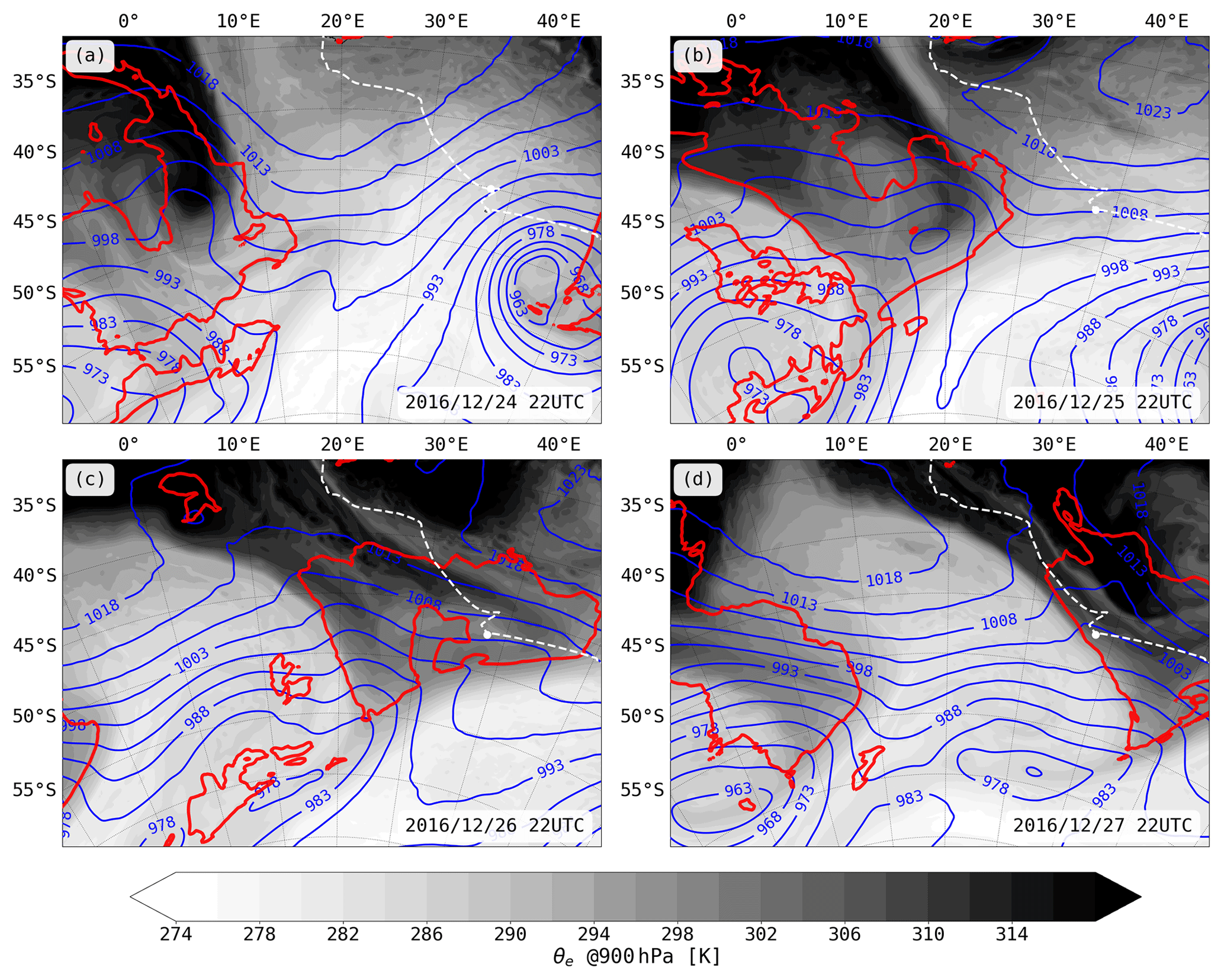
Figure 5Horizontal cross sections of equivalent potential temperature at 900 hPa (θe @900 hPa) and sea level pressure (blue contours, in hPa) at four time steps during the warm advection case study. The white dashed line shows the ACE ship track, and the white dot denotes the position of the research vessel. The red contours show that warm temperature advection mask (see Sect. 4.1 for details).
4.1 Synoptic overview
The warm sector of an extratropical cyclone passes south of Marion Island (white dot in Fig. 5b–d) from 24 to 28 December 2016. At 22:00 UTC on 25 December 2016, this cyclone is positioned at 5∘ W and 55∘ S. While the cyclone centre is already uniformly cold, it is associated with prominent warm and cold fronts that meet near 25∘ E and 50∘ S. Both fronts are visible by clear kinks in the sea level pressure contours and sharp gradients in equivalent potential temperature (θe) at 900 hPa indicating a transition zone between two air masses, i.e. dry and cold air mass with low θe and warm and moist air masses with high θe (see Schemm et al., 2017 for a discussion on objective midlatitude front identification). The focus of this study is the wide warm sector spanned by these fronts. An elongated band of high θe (see Fig. 5a, b) leads to the highest θe values behind the warm front between 22:00 UTC on 25 and 26 December 2016. A second area of high θe is located ahead of the cold front (see Fig. 5b, c). These two regions of high θe are separated by a weak secondary warm front at 22:00 UTC on 26 December 2016 associated with a short-lived meso-cyclone forming and dissolving on 25 December (see weak low-pressure system at 52∘ S and 18∘ E in Fig. 5b). The strongest precipitation is seen along the cold and warm front and, towards the end of the case study, along the occluded front, which forms around 25∘ E and 50∘ S on 26 December 2016 (see Supplement Fig. S2c). Weak, shallow-convective precipitation occurs in the cold sector. The region of the warm sector is defined by the near-surface air–sea temperature difference as described in Thurnherr et al. (2021). If the difference between the 2 m air temperature and the sea surface temperature is above 1 ∘C, the region is associated with the advection of warm and moist air defining the warm temperature advection mask indicated by the red contours in Fig. 5. The warm sector region encompasses a triangular region in between the cold and warm front, which is dominated by warm temperature advection. When referring to the warm sector in the following, we are referring to this area of warm temperature advection.
The ACE measurements for this case study were taken at Marion Island, where the research vessel was anchored during the cyclone passage (black dot in Fig. 5). The vessel stayed in the warm sector for 36 h. A good agreement of measured and simulated hs and qa can be seen (Fig. 6). The simulated precipitation compares well with the measurements on 26 December but is shifted and shows lower intensity on 27 December 2016, during which enhanced precipitation is measured around 06:00 UTC, while simulated precipitation occurs after 12:00 UTC with lower intensity. This shift and underestimation led to too low hs and qa in the simulation in this time period. Measured hs stays above 1.0 for nearly the entire event from 15:00 UTC on 26 December to 00:00 UTC on 28 December 2016 (Fig. 6b). Simultaneously, simulated ocean evaporation is negative, indicating dew deposition on the ocean surface (Fig. 6c). The highest dew deposition rates coincide with high hs and qa and a very shallow diagnosed boundary layer height in the model as expected in stable near-surface conditions. There are two peaks in dew deposition rates at the measurement site, which correspond to two areas of high θe within the warm sector (Fig. 5). The first area of dew deposition lies behind the warm front and the second ahead of the cold front. In between these two areas, weakly positive ocean evaporation occurs (Fig. 6c). This specific structure of hs and θe in the warm sector is imprinted in the isotopic composition of the near-surface water vapour. The distribution and evolution of SWIs in the warm sector during the case study are discussed in the next section.
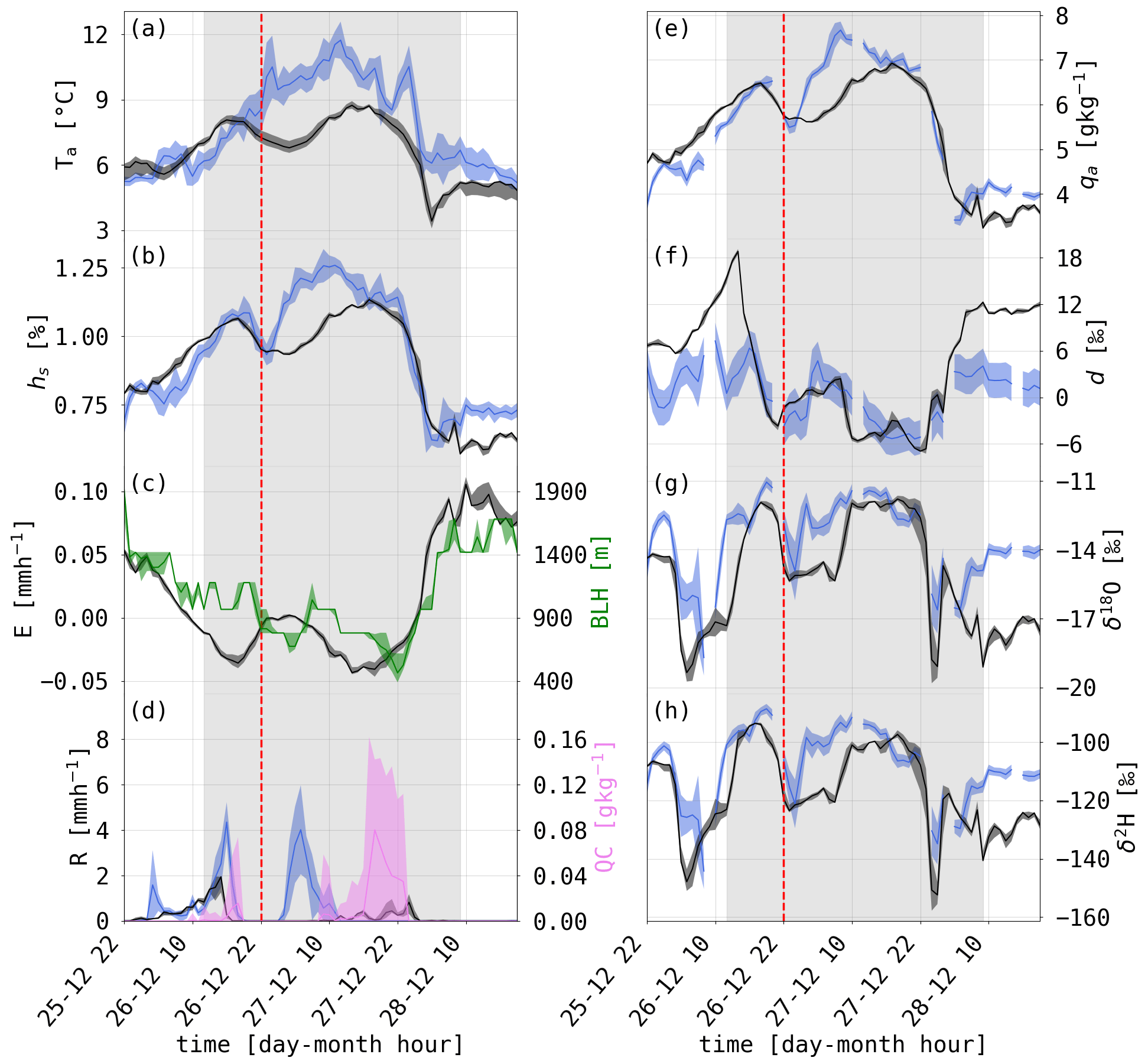
Figure 6Time evolution of hourly (a) air temperature Ta, (b) hs, (c) ocean evaporation E (positive upward) and boundary layer height BLH (green), (d) precipitation rate R and mean cloud water content on the five lowest model levels (10–200 m a.s.l.) (QC), (e) specific humidity (qa), (f) d, (g) δ18O, and (h) δ2H from ACE measurements and COSMOiso simulations interpolated along the ship track during the warm temperature advection event at Marion Island from 26 to 28 December 2016. The blue lines show the measurements with hourly standard deviation; the black, green and pink lines show the simulated values including the variability from 10∘ latitudinal and longitudinal shifts of the ACE track (black, green and pink areas). The vertical red dashed line denotes 22:00 UTC on 26 December 2016. The shaded grey areas correspond the time period of the warm temperature advection event.
4.2 Isotope signals
The measured isotopic composition of water vapour during the cyclone passage shows a decrease of 10 ‰ in d to −5.4 ‰ and an increase in δ18O of 5 ‰ and δ2H of 30 ‰ up to −11 ‰ and −88 ‰, respectively (Fig. 6f–h). The simulated timelines of d, δ18O and δ2H agree qualitatively and quantitatively well with the measurements in the warm sector showing a Pearson correlation above 0.7 for all isotope variables and a mean absolute error of 3.6 ‰, 1.4 ‰ and 9.6 ‰, respectively. This good agreement of SWIs in COSMOiso and the ACE measurements allows for further analysis of the SWI evolution in the COSMOiso simulation for this case study. Possible reasons for deviations were discussed in Thurnherr et al. (2021), with the choice of a too strong non-equilibrium fractionation factor for ocean evaporation and dew formation being the most important one.
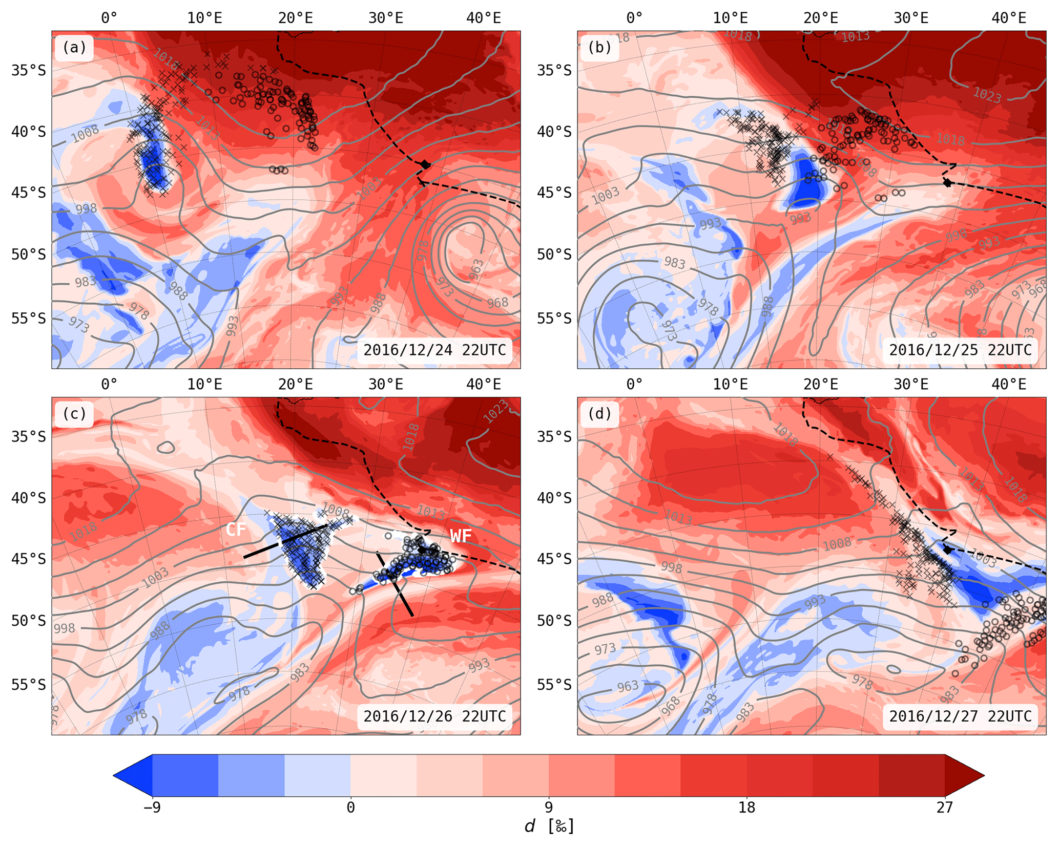
Figure 7Panels (a)–(d) show horizontal cross sections of d at the lowest model level and sea level pressure (grey contours, in hPa) at four time steps during the warm advection case study. The black dashed line shows the ACE ship track, and the black square denotes the position of the research vessel. The white framed regions in panel (c) show the starting regions WF and CF of the backward and forward trajectories at 22:00 UTC on 26 December 2016. Circles and crosses in panels (a)–(d) show the position of trajectories starting below 50 m a.s.l. in the regions WF and CF, respectively. The black solid lines in panel (c) denote the positions of the vertical cross section across the cold and warm front, respectively, in Fig. 8.
As shown in Fig. 7, the development of d during the cyclone's passage is characterised by negative d close to the cyclone centre and along the fronts in the warm sector, clearly visible at 22:00 UTC on 26 December 2016 (white contours in Fig. 7c). These two Eulerian features are confined to the areas behind the warm front and ahead of the cold front, respectively. In between the low-d regions, there is a region of d above 0 ‰ overlapping with the region of low θe in the warm sector (Fig. 5c). The low-d region behind the warm front (region WF) shows continuously low d below −9 ‰ and stays situated in a region of warm advection within the warm sector from 24 to 27 December. The low-d region ahead of the cold front (region CF) is more variable in sign, shape and position than the warm-frontal low-d region. d decreases in region CF during the four days of the case study, from values mainly above −6 ‰ to values below −9 ‰. Shortly after the dissolution of the short-lived meso-cyclone, the area of region CF increases from a confined region close to the cold front to a larger triangular region spanning towards the middle of the warm advection mask incorporating the warm sector of the meso-cyclone (compare Fig. 7b and c).
Additionally to the evolution of these Eulerian d features during the case study, the position of backward and forward trajectories starting below 50 m a.s.l. from these two low-d regions in the warm sector at 22:00 UTC on 26 December 2016 are shown in Fig. 7 (see also Supplement Fig. S3 for the full trajectory paths). By construction, at 22:00 UTC on 26 December 2016 (Fig. 7c) all trajectories lie within the regions CF and WF. The backward trajectories entered the marine boundary layer at latest 84 h before arrival in the low-d regions (see Supplement Fig. S1d), which they enter only a few hours before arrival. Most strikingly, the trajectories entering region WF resided in a region of very high d above 20 ‰ a day before arrival (circles in Fig. 7b). Therefore, these trajectories experience a strong decrease in d within 24 h before arrival in region WF. Similarly, the trajectories arriving ahead of the cold front enter region CF within the 24 h before arrival. Furthermore, the back trajectories arriving in region CF were located in a region of low d 48 h before arrival (Fig. 7a) also coming from a region of high d with values above 20 ‰ 72 h before arrival in region CF (see Supplement Fig. S1a). The low-d regions in the lower MBL are therefore constantly rebuilt by newly arriving trajectories, which saw a decrease in d just shortly before arrival in the low-d regions. This indicates that the low d in these Eulerian features is not materially conserved but constantly renewed. Fast changes in d are therefore important to keep these low d features in the lower MBL alive, and the single-process APMs can help to identify the processes leading to these strong and rapid decreases in d.
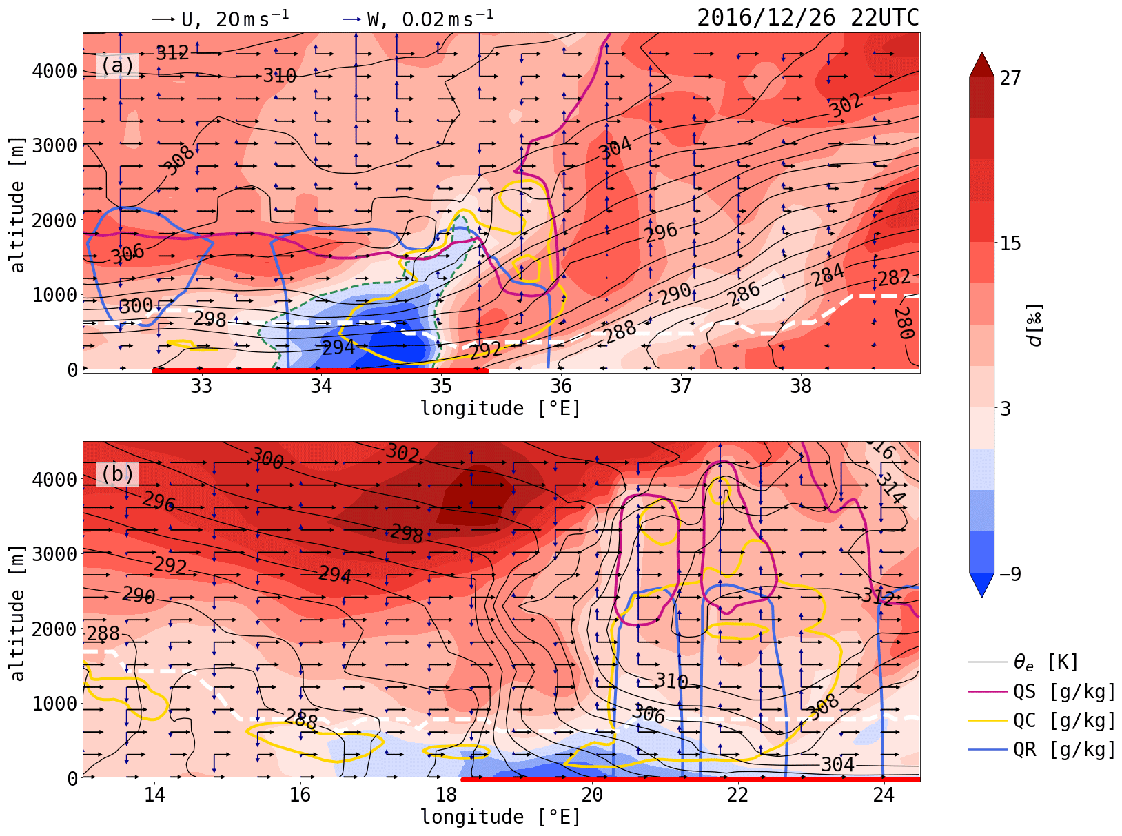
Figure 8Vertical cross sections of d across the (a) warm front and (b) cold front at 22:00 UTC on 26 December 2016. The equivalent potential temperature (θe, black contours), the snow water content (QS, pink frame), the cloud water content above 0.1 g kg−1 (QC, yellow frame), the rain water content above 0.005 g kg−1 (QR, blue frame), the boundary layer height (white, dashed line), and horizontal (U, black) and vertical (W, blue) wind vectors are shown. The red lines at the bottom of the panels show the regions of warm temperature advection. The orientation of the cross sections is shown in Fig. 7c.
So far, we only discussed the d patterns on the lowest model level at approximately 10 m.a.s.l. A vertical cross section of d across the cold and warm front at 22:00 UTC on 26 December 2016 is shown in Fig. 8 to illustrate the vertical extent of these near-surface low-d regions. Occurrences of low d behind the warm front lie entirely within the warm advection region and behind the strong temperature gradient across the warm front (Fig. 8a). The lowest d values occur in the lower MBL and directly along the warm front. In contrast to the cold front, low d is also seen above the MBL. The area of low d might extend to higher altitudes due to the strong vertical wind shear at lower levels inducing turbulence, despite the stable stratification and leading to vertical mixing (low bulk Richardson numbers can be observed in this region, not shown). In the upper MBL behind the warm front, the low d values might be further transported upward and eastward by large-scale advection. This is supported by the wind patterns in the low-d region and highlights the importance of vertical mixing combined with large-scale transport in the frontal region to shape the d distribution in water vapour. Rain and cloud water are present for most of the low-d region behind the warm front. Across the cold front, low d is confined to the lower MBL and covers a region which mainly overlaps with warm advection but which also spreads towards the cold side of the front (see negative d west of 18∘ E in Fig. 8b). The cold front does not show a typical temperature gradient with increasing θe towards the warm sector and with height. A weak temperature gradient is visible close to surface between 19 an 21∘ E. An upper-level cold front can be observed above 2000 m. Two precipitation cells with strong showers are present at the eastern edge of the low-d region, while the lowest d values are located in cloud- and rain-free areas.
The evolution of δ18O and δ2H in the warm sector shows a pattern opposite to d. Due to the similarity of the variability in δ18O and δ2H only a description of δ18O is given in the following. δ18O shows larger values in the warm sector, with the highest values lying in the regions CF and WF (see Supplement Fig. S4). A prominent feature is very low δ18O values along the fronts showing the imprint of frontal precipitation along the warm front (and less strongly along the cold front), most likely due to below-cloud interaction. These low-δ18O regions overlap with regions of high d.
To understand which processes are most important for these specific isotopic patters and especially for the low d values seen in the warm sector, the evolution of SWIs in water vapour is analysed by using the COSMOiso trajectories and by applying the single-process APMs in the following.
4.3 Application of the single-process APMs along the COSMOiso trajectories
The single-process APMs introduced in Sect. 3 simulate the effect of three processes on the isotopic composition of water vapour in an air parcel during transport: (1) decreasing d due to ocean evaporation during the movement over a negative SST gradient is simulated with APMevap. (2) If the air parcel becomes supersaturated (hs>1.0), d decreases due to dew deposition, which is simulated with APMdew. (3) The formation of cloud droplets during a moist-adiabatic ascent of an air parcel can also lead to a decrease in d as simulated with APMray. In the following, the d evolution along COSMOiso trajectories is compared to these APM simulations to assess if the single-process APMs are able to simulate the specific changes in d seen along the COSMOiso trajectories.
The evolution of SWIs along the trajectories together with the APM evolutions is studied in d–qa and d–δ18O phase space diagrams (see Fig. 2). Figure 9a and c show the evolution of d and qa along 4 d trajectories arriving in region WF. Four days before arrival, these trajectories were situated in an evaporative environment and experienced an increase in d and qa simultaneously with increasing ocean evaporation. d peaks, on average, 34 h before arrival and starts to decrease while qa is still increasing. On average, 18 h before arrival, qa peaks and starts decreasing thereafter. Shortly before arrival, some trajectories see again an increase in d by a few per mille to a final d of −4.8 [−8.4, −2.0] ‰ (the brackets denote the 25th to 75th percentile range). The trajectories arriving in region CF (Fig. 9b, d) show a similar d and qa evolution in the 4 d before arrival as the ones arriving in region WF. The main differences are a higher maximum in qa and two local minima in d. A first minimum in d is seen, on average, 40 h before arrival when the trajectories pass the low-d region behind the warm front in the warm sector of the forming meso-cyclone (compare Figs. 5a and 7a). A second minimum occurs upon arrival when the trajectories enter the low-d region ahead of the cold front.
The variations in d and δ18O along the trajectories follows specific patters, which are also seen in idealised APM simulations. The decrease in d while qa is still increasing follows a similar pattern as seen with the APMevap (dashed lines in Fig. 9c, d). The following decrease in d with a simultaneous decrease in qa follows a similar pattern as the idealised APMdew simulations (solid lines in 9c, d). These idealised simulations use a prescribed qa and SST evolution as introduced in Sect. 3.1 and 3.2. For both APMevap and APMdew, the idealised simulations show a similar behaviour in the qa–d phase space as the trajectories but do not cover the entire range of values simulated along the COSMOiso trajectories. In particular, the lowest d values along the trajectories are not reproduced by the idealised APM simulations. AMPray (dotted lines in Fig. 9c, d) simulations show a too weak decrease in d to explain changes in d and qa along the trajectories arriving in regions WF and CF.
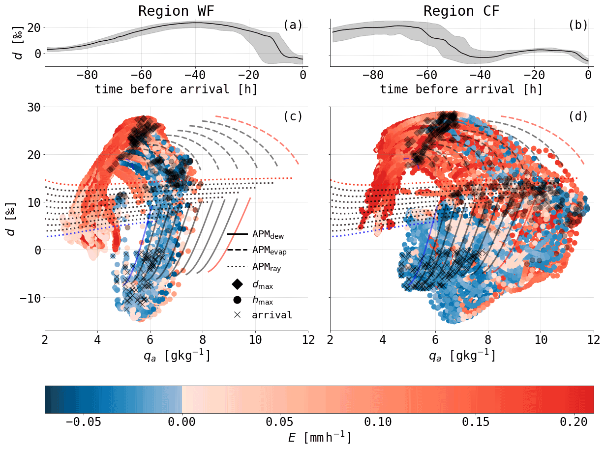
Figure 9Evolution of d (median and [25, 75] percentile range) along 4 d backward trajectories starting at 22:00 UTC on 26 December 2016 below 50 m (a) behind the warm front (region WF) and (b) ahead of the cold front (region CF). Phase space diagrams of d versus qa for (c) region WF and (d) region CF (hourly values along the trajectories are shown by dots, coloured by ocean evaporation (E), which is defined positive upward). The results of the APMs are shown by black lines, solid for APMdew, dashed for APMevap and dotted for APMray. The red lines show the simulations with the highest SST (Ta for APMray) and the blue lines with the lowest. For details on the model setups, see Appendix Table B1 and text. Markers denote specific events along the trajectories: the time of highest d (black diamond), the time of highest hs (black dot) and the time of arrival at the measurement site (black cross).
The assumed, idealised SST and qa evolution in the APM simulations might lead to the difference between the APMs and the COSMOiso trajectories. Instead of these idealised assumptions, the evolution of qa and SST along the COSMOiso trajectories arriving in region WF is used for APMevap and APMdew simulations shown in Fig. 10a. Δqa in these APM simulations is defined as the change in qa during a 1-hourly time step along the COSMOiso trajectories. APMevap simulations start at the time of highest d for each trajectories and run until hs>0.9. APMdew simulations are initiated at the first time step of h>1.02 and run until hs<1.005. Additionally, if the trajectory ascends above 50 m a.s.l., the APM simulation is ended. With the SST and qa evolution from the COSMOiso trajectories, the APMevap simulation covers the entire range of simulated d values in the COSMOiso simulations. Similarly, APMdew simulates lower d values than in the prescribed simulations.
The changes relative to the initial values for d (Δd) and δ18O (Δδ18O) during these APM simulations versus the changes along the corresponding trajectories are shown in Fig. 10b–e. Δδ18OAPM agrees well with Δδ18Otraj for both APM simulations with a larger spread for APMdew. While Δd agrees well for APMdew, Δd shows a weaker decrease by a few per mille in the APMevap simulations compared to the trajectories.
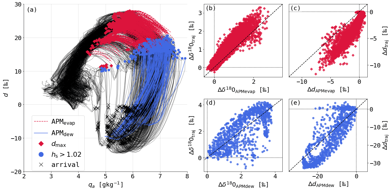
Figure 10(a) Same as Fig. 9c but showing trajectories as black lines and the corresponding APMdew (blue solid lines) and APMevap (pink dashed lines) simulations using the SST and qa evolution of the COSMOiso trajectories. Markers denote specific events along the trajectories: the starting position of APMevap at highest d (pink diamond), the starting position of APMdew at the first instance when h>1.02 along the trajectories (blue dot) and the arrival of the trajectories (black cross). Comparisons of changes in δ18O (b, d) and d (c, e) along COSMOiso trajectories (traj) and during the corresponding APMevap (b, c) and APMdew (d, e) simulations are shown. The changes in δ18O and d are shown relative to the initial composition of the APM simulations in 1-hourly resolution.
The application of the single-process APMs shows that the decrease in d along the near-surface COSMOiso trajectories arriving in the warm sector is dominated by two processes: (1) ocean evaporation and (2) dew deposition during a movement over a negative SST gradient in the warm sector of a midlatitude cyclone. Thus, the water vapour fluxes at the ocean–atmosphere interface can explain most of the d signal in water vapour along the trajectories. The remaining differences between the trajectories and APM simulation can have several causes. With the single-process APMs, only one process is taken into account at a time. In reality and in COSMOiso, the air parcel can be influenced by more than a single process at a time, leading to complex non-linear interactions between the different processes at play. For example, turbulent and vertical transport during ocean evaporation can mix water vapour with a different isotopic composition into the air parcel. This can be expected during strong ocean evaporation in a vertically unstable atmosphere and plays a role in an evaporative environment, as for example in the subtropics (Benetti et al., 2014). In APMevap such conditions are mainly given in the beginning of the simulation when hs is low and strong ocean evaporation occurs in a conditionally unstably stratified MBL. The underestimation of the decrease in d in the APMevap simulations could thus be caused by neglecting the mixing of the air parcel's water vapour with surrounding water vapour. In the supersaturated environment during dew deposition, the atmosphere is generally stably stratified. Still, due to the strong vertical wind shear, turbulence can be produced even in this stably stratified environment and might have caused vertical mixing in the warm sector's MBL. While upward turbulent transport could explain the vertical extent of the negative d anomaly, strong vertical mixing rather counteracts the formation of low d near the ocean surface by mixing high d from the free troposphere downward. Thus, other processes have to be considered to explain the difference between the APMdew simulations and the COSMOiso trajectories. Below-cloud processes such as the evaporation of rain droplets or the equilibration of rain droplets with the surrounding water vapour might affect SWIs in the warm sector. If the rain droplets have experienced substantial evaporation beforehand, d of the rain droplets is expected to be low due to non-equilibrium fractionation during evaporation. This can introduce low d into the MBL during precipitation. The near-surface trajectories of this study do not show different isotopic signals under the presence of cloud or rain water than without the presence of hydrometeors (not shown). The observed, relatively small differences between the APMdew simulations and the COSMOiso trajectories might therefore be a result of non-linear effects of the combination of several processes such as altering periods of ocean evaporation and dew deposition, variations in the ocean water's isotope composition, and below-cloud and mixing processes.
The aim of this study was to better understand the processes leading to characteristic water vapour SWI signals observed in the warm sector of extratropical cyclones using air parcel process models. As shown in a previous study based on a statistical analysis, dew deposition on the ocean surface, Rayleigh fractionation during cloud formation and weakening ocean evaporation mainly shape the isotopic composition of water vapour in the warm sector (Thurnherr et al., 2021). Here, we further investigate these processes in a mechanistic way by simulating the specific SWI evolution due to different moist processes using single-process APMs of ocean evaporation and dew deposition on the ocean surface, when moving across a meridional SST gradient and Rayleigh fractionation during a moist-adiabatic ascent. These simple process models adequately simulate the SWI evolution along COSMOiso backward trajectories and confirm the main processes identified in the case study of warm temperature advection in a Southern Ocean cyclone. Furthermore, these APMs give an estimate of the induced changes in d, δ18O, δ2H and q by the represented processes.
The strongest changes in water vapour d are caused by the modulation of air–sea fluxes such as decreasing ocean evaporation during the movement across an SST gradient towards lower SSTs and dew deposition, which can both lead to a decrease in d on the order of 10‰. Air–sea interactions and especially the change in d depend strongly on hs. For ocean evaporation, the evolution of hs is affected by the strength of the ocean evaporation and the SST. The higher hs at maximum SST is, the lower the maximum d gets and, thus, the stronger the decrease in d becomes. The decrease in d during dew deposition is mostly influenced by the initial supersaturation, which determines the strength of the non-equilibrium fractionation. The SST gradient determines the decrease in d during dew deposition by determining how quickly saturation is reached. Rayleigh fractionation during a moist-adiabatic ascent can lead to a decrease in water vapour d 1 order of magnitude smaller than the air–sea interactions and is mainly governed by the initial temperature. The APMs illustrate the unique pathways associated with the simulated processes in the d–δ18O and d–qa, which can therefore be used to identify these processes along trajectories.
The introduced process models simplify the reality by only showing the effect of one process for each model. Furthermore, effects from changes in the SST and ocean skin layer SWI composition due to the air–sea interactions are neglected. Despite these caveats, the process models are able to reproduce the SWI evolution along trajectories for time periods when one moist process dominates the SWI variability.
Compared to previous Eulerian process models, which simulated the SWI composition of the MBL and mainly investigated the effect of vertical moisture transport (e.g. Merlivat and Jouzel, 1979; Benetti et al., 2018; Feng et al., 2019), the Lagrangian perspective used here is important to understand the SWI variability in the extratropics, where the large-scale horizontal advection is 1–2 orders of magnitude larger than the vertical advection, and therefore strongly affects the SWI variability of water vapour. Previous studies have used Lagrangian approaches to model the SWI variability of water vapour. Pfahl and Wernli (2009) integrated the evaporated water vapour from ocean evaporation at the moisture sources along trajectories to compare with measurements of SWIs in water vapour at the coast. We adapted this approach to more idealised situations of ocean evaporation across an SST gradient with APMevap, which helps to understand the main factors influencing the SWI evolution during continuous ocean evaporation.
Rayleigh fractionation models have frequently been used to simulate the effect of continuous rainout on the isotopic composition of water vapour and precipitation arriving over land (e.g. Helsen et al., 2006; Galewsky et al., 2007; Bonne et al., 2014). With the APMray, we highlight that Rayleigh fractionation during a moist-adiabatic ascent can potentially lead to low d in MBL water vapour due to the temperature dependency of the equilibrium fractionation factors with distinctly different changes in SWIs and qa than air–sea interaction.
Dütsch et al. (2018) used trajectories calculated from COSMOiso simulations to identify contributions of different processes to the SWI composition of water vapour over Europe. This identification method based on changes of qa and h along the trajectory gave detailed insight into the SWI variability over Europe. In this study we looked at each process from a mechanistic perspective and identified additional important processes in the MBL such as dew deposition. This study therefore helps to better constrain processes affecting the isotopic composition of water vapour over the ocean surface before the air parcel moves over terrestrial surfaces.
The case study of a warm temperature advection event showed that negative d in near-surface water vapour in the warm sector of extratropical cyclones is primarily a result of air–sea interactions. Moreover, the decrease in d occurs shortly before arrival of the trajectories after the air parcels experienced an increase in d in an evaporative environment. These fast and strong changes in d upon arrival in the warm sector show that the low-d regions are not materially conserved but are constantly rebuilt by newly arriving trajectories, which has two major implications for future studies.
-
First, this means that measurements of SWIs in water vapour close to the ocean surface, as for example conducted on research vessels, are good tracers of local to regional air–sea interactions. This has also been shown for ocean evaporation and vertical mixing processes with measurements of SWIs in the subtropical Atlantic MBL (Benetti et al., 2015). Here, we show that in the extratropics, d in MBL water vapour changes quickly during transport due to air–sea moisture fluxes in either direction, i.e. due to ocean evaporation or dew deposition. These local air–sea interactions in extratropical cyclones, which are strongly driven by the large-scale temperature advection, dominate the d variability in water vapour close to the ocean surface and overwrite the advected d signal.
-
Second, while d in water vapour close to the surface changes quickly from a Lagrangian perspective, the Eulerian signal is more persistent and shows low d up to and above the MBL top. The low d signal in the upper MBL might be a result of vertical mixing due to strong vertical wind shear. In the upper MBL, large-scale advection of d might be more important than close to the ocean surface. To further study these complex vertical interactions of mixing and large-scale advection in the warm sector, the methods used here need to be supplemented by modelling methods that explicitly include mixing processes such as process tagging (Fiorella et al., 2021) or isotope tendencies in isotope-enabled numerical weather prediction models. Such methods would allow us to thoroughly investigate the role of mixing for the advection of low d in and above the MBL. Furthermore, such modelling approaches have to be combined with aircraft or drone-based high-resolution vertical measurements of the vapour SWI composition. Such observations are indispensable to better constrain the processes affecting the upper part of the marine boundary layer at cloud base and in the cloud layer.
In summary, this study confirms and emphasises that the isotopic composition of near-surface water vapour is not only affected by ocean evaporation at the moisture source, but also by other processes, in particular dew deposition, during transport. These processes are a results of the specific path of individual air parcels and the evolution of SST and hs during transport by the large-scale atmospheric flow. It is the combination of observational and modelling data sets that allows us to conduct such in-depth process-based analysis of MBL moisture cycling under the influence of large-scale flow patterns. In the future, this type of analysis could be used to quantify the contribution of single processes to the SWI variability in the cold and warm sector of extratropical cyclones or to assess the lifetime of negative d in the MBL to quantify the effect of low d in near-surface water vapour on the isotopic composition of precipitation in the Southern Ocean and on Antarctica. Furthermore, the presented process models can be applied in various environmental settings to study the role of surface–atmosphere exchange processes influencing SWI variability along the large-scale flow.
A1 Model setup
We initiate an air parcel with a specific humidity and a supersaturation of , where qs is the saturation specific humidity at SST. We assume that this air parcel only interacts with the ocean surface and does not exchange water vapour with its atmospheric environment. We let this air parcel equilibrate with the ocean surface by iteratively decreasing qa by an amount Δqa through dew deposition. Using the traditional bulk aerodynamic formulation, the depositional fluxes for the light water vapour lE and the heavy water vapour hE can be formulated as follows:
where Ψ=ρλCe U, with ρ the air density, λ the latent heat of vaporisation, Ce a non-dimensional transfer coefficient and U the wind speed at 10 m a.s.l.; αk≤1 the non-equilibrium fractionation factor; hqa the specific humidity of the heavy water molecules; and hqs the saturation specific humidity of the heavy water molecules.
Equations (A1) and (A2) can be combined to get an expression of the isotopic ratio of the depositional flux Rflux. Including the boundary condition that hqs is equal to the saturation specific humidity at SST, , where αe<1 is the equilibrium fractionation factor. Replacing hqa by Ra⋅qa, we get the following equation:
Equation (A3) corresponds to the equation for the isotopic ratio of the evaporation flux of the CG65 model.
The isotopic composition of the water vapour is iteratively calculated with
and thus the isotope ratio of the vapour in the air parcel can be calculated as
For Fig. 9 the following APM setups are used: for each APM 10 different simulations are conducted, which are summarised in Table B1. All simulation are initialised at a pressure of 1000 hPa. APMevap is stopped if hs increases above 0.9, APMdew is stopped if hs<1.04 and APMray is stopped if less than 2% of the initial moisture remains in the air parcel.

The Python code of the air parcel process models is published on Zenodo: https://doi.org/10.5281/zenodo.6979911 (Thurnherr and Aemisegger, 2022).
The ACE data sets are published on the Zenodo research data repository: https://zenodo.org/communities/spi-ace/ (Thomas, 2022). The isotopic composition of water vapour during ACE is available with the DOI https://doi.org/10.5281/zenodo.3250790 (Thurnherr and Aemisegger, 2020). The rainfall data sets are published with the DOI https://doi.org/10.5281/zenodo.3929289 (Gehring et al., 2020), the sea surface temperature data set is published with the DOI https://doi.org/10.5281/zenodo.3660852 (Haumann et al., 2020), and the meteorological data set is published with the DOI https://doi.org/10.5281/zenodo.3379590 (Landwehr et al., 2019). The COSMOiso simulations are available on the ETH Research Collection with the DOI https://doi.org/10.3929/ethz-b-000445744 (Thurnherr et al., 2020b).
The supplement related to this article is available online at: https://doi.org/10.5194/acp-22-10353-2022-supplement.
This paper is part of IT's PhD thesis. IT and FA designed the study; IT carried out the simulations, performed the analyses and wrote the paper with feedback from FA. Both authors discussed the results.
The contact author has declared that neither of the authors has any competing interests.
Publisher’s note: Copernicus Publications remains neutral with regard to jurisdictional claims in published maps and institutional affiliations.
ACE was a scientific expedition carried out under the auspices of the Swiss Polar Institute, supported by funding from the ACE Foundation and Ferring Pharmaceuticals. The COSMOiso simulations were performed at the Swiss National Supercomputing Centre (CSCS) with the small production projects sm08 and sm32. The authors gratefully acknowledge Heini Wernli (ETH Zurich) for helpful discussions and his feedback on a previous version of the manuscript, Stephan Pfahl (Freie Universität Berlin) for his feedback on the single-process air parcel models definition, and Adriana Bailey (NCAR Boulder) for her input on the inter-comparison between the single-process air parcel models (Fig. 2). We thank the two anonymous reviewers for their valuable input to the paper.
This research has been supported by the Swiss Polar Institute (GLACE project DAWATEC and ACE project 11), Ferring Pharmaceuticals (ACE project 11) and the Fondation BNP Paribas (ACE project 11).
This paper was edited by Thorsten Bartels-Rausch and reviewed by two anonymous referees.
Aemisegger, F.: On the link between the North Atlantic storm track and precipitation deuterium excess in Reykjavik, Atmos. Sci. Lett., 19, e865, https://doi.org/10.1002/asl.865, 2018. a
Aemisegger, F. and Papritz, L.: A climatology of strong large-scale ocean evaporation events, Part I: Identification, global distribution, and associated climate conditions, J. Clim., 31, 7287–7312, https://doi.org/10.1175/JCLI-D-17-0591.1, 2018. a
Aemisegger, F. and Sjolte, J.: A climatology of strong large-scale ocean evaporation events, Part II: Relevance for the deuterium excess signature of the evaporation flux, J. Clim., 31, 7313–7336, https://doi.org/10.1175/JCLI-D-17-0592.1, 2018. a, b
Aemisegger, F., Sturm, P., Graf, P., Sodemann, H., Pfahl, S., Knohl, A., and Wernli, H.: Measuring variations of δ18O and δ2H in atmospheric water vapour using two commercial laser-based spectrometers: An instrument characterisation study, Atmos. Meas. Tech., 5, 1491–1511, https://doi.org/10.5194/amt-5-1491-2012, 2012. a
Aemisegger, F., Spiegel, J. K., Pfahl, S., Sodemann, H., Eugster, W., and Wernli, H.: Isotope meteorology of cold front passages: A case study combining observations and modeling: Water isotopes during cold fronts, Geophys. Res. Lett., 42, 5652–5660, https://doi.org/10.1002/2015GL063988, 2015. a
Beare, R. J.: Boundary layer mechanisms in extratropical cyclones, Q. J. R. Meteorol. Soc., 133, 503–515, https://doi.org/10.1002/qj.30, 2007. a, b
Benetti, M., Reverdin, G., Pierre, C., Merlivat, L., Risi, C., Steen-Larsen, H. C., and Vimeux, F.: Deuterium excess in marine water vapor: Dependency on relative humidity and surface wind speed during evaporation, J. Geophys. Res.-Atmos., 119, 584–593, https://doi.org/10.1002/2013JD020535, 2014. a, b
Benetti, M., Aloisi, G., Reverdin, G., Risi, C., and Sèze, G.: Importance of boundary layer mixing for the isotopic composition of surface vapor over the subtropical North Atlantic Ocean, J. Geophys. Res.-Atmos., 120, 2190–2209, https://doi.org/10.1002/2014JD021947, 2015. a
Benetti, M., Lacour, J.-L., Sveinbjörnsdóttir, Á. E., Aloisi, G., Reverdin, G., Risi, C., Peters, A. J., and Steen-Larsen, H. C.: A framework to study mixing processes in the marine boundary layer using water vapor isotope measurements, Geophys. Res. Lett., 45, 2524–2532, https://doi.org/10.1002/2018GL077167, 2018. a, b, c
Blossey, P. N., Kuang, Z., and Romps, D. M.: Isotopic composition of water in the tropical tropopause layer in cloud-resolving simulations of an idealized tropical circulation, J. Geophys. Res.-Atmos., 115, D24309, https://doi.org/10.1029/2010JD014554, 2010. a
Bond, N. A. and Fleagle, R. G.: Prefrontal and postfrontal boundary layer processes over the ocean, Mon. Weather Rev., 116, 1257–1273, https://doi.org/10.1175/1520-0493(1988)116<1257:PAPBLP>2.0.CO;2, 1988. a
Bonne, J.-L., Masson-Delmotte, V., Cattani, O., Delmotte, M., Risi, C., Sodemann, H., and Steen-Larsen, H. C.: The isotopic composition of water vapour and precipitation in Ivittuut, southern Greenland, Atmos. Chem. Phys., 14, 4419–4439, https://doi.org/10.5194/acp-14-4419-2014, 2014. a
Boutle, I. A., Beare, R. J., Belcher, S. E., Brown, A. R., and Plant, R. S.: The moist boundary layer under a mid-latitude weather system, Bound.-Lay. Meteorol., 134, 367–386, https://doi.org/10.1007/s10546-009-9452-9, 2010. a
Craig, H. and Gordon, L. I.: Deuterium and oxygen 18 variations in the ocean and the marine atmosphere, in: Stable Isotopes in Oceanographic Studies and Paleotemperatures, edited by: Tongiorgi, E., 9–130, Lab. Geol. Nucl., Pisa, Italy, 1965. a, b, c, d
Dahinden, F., Aemisegger, F., Wernli, H., Schneider, M., Diekmann, C. J., Ertl, B., Knippertz, P., Werner, M., and Pfahl, S.: Disentangling different moisture transport pathways over the eastern subtropical North Atlantic using multi-platform isotope observations and high-resolution numerical modelling, Atmos. Chem. Phys., 21, 16319–16347, https://doi.org/10.5194/acp-21-16319-2021, 2021. a, b
de Vries, A. J., Aemisegger, F., Pfahl, S., and Wernli, H.: Stable water isotope signals in tropical ice clouds in the West African monsoon simulated with a regional convection-permitting model, Atmos. Chem. Phys., 22, 8863–8895, https://doi.org/10.5194/acp-22-8863-2022, 2022. a
Dütsch, M., Pfahl, S., and Wernli, H.: Drivers of δ2H variations in an idealized extratropical cyclone, Geophys. Res. Lett., 43, 5401–5408, https://doi.org/10.1002/2016GL068600, 2016. a
Dütsch, M., Pfahl, S., and Sodemann, H.: The impact of nonequilibrium and equilibrium fractionation on two different deuterium excess definitions, J. Geophys. Res.-Atmos., 122, 12732–12746, https://doi.org/10.1002/2017JD027085, 2017. a, b
Dütsch, M., Pfahl, S., Meyer, M., and Wernli, H.: Lagrangian process attribution of isotopic variations in near-surface water vapour in a 30-year regional climate simulation over Europe, Atmos. Chem. Phys., 18, 1653–1669, https://doi.org/10.5194/acp-18-1653-2018, 2018. a, b
Dütsch, M., Blossey, P. N., Steig, E. J., and Nusbaumer, J. M.: Nonequilibrium fractionation during ice cloud formation in iCAM5: Evaluating the common parameterization of supersaturation as a linear function of temperature, J. Adv. Model Earth Sy., 11, 3777–3793, https://doi.org/10.1029/2019MS001764, 2019. a
Eckstein, J., Ruhnke, R., Pfahl, S., Christner, E., Diekmann, C., Dyroff, C., Reinert, D., Rieger, D., Schneider, M., Schröter, J., Zahn, A., and Braesicke, P.: From climatological to small-scale applications: simulating water isotopologues with ICON-ART-Iso (version 2.3), Geosci. Model Dev., 11, 5113–5133, https://doi.org/10.5194/gmd-11-5113-2018, 2018. a
Feng, X., Posmentier, E. S., Sonder, L. J., and Fan, N.: Rethinking Craig and Gordon's approach to modeling isotopic compositions of marine boundary layer vapor, Atmos. Chem. Phys., 19, 4005–4024, https://doi.org/10.5194/acp-19-4005-2019, 2019. a
Fiorella, R. P., Siler, N., Nusbaumer, J., and Noone, D. C.: Enhancing Understanding of the Hydrological Cycle via Pairing of Process-Oriented and Isotope Ratio Tracers, J. Adv. Model. Earth Syst., 13, e2021MS002648, https://doi.org/10.1029/2021MS002648, 2021. a
Galewsky, J., Strong, M., and Sharp, Z. D.: Measurements of water vapor D/H ratios from Mauna Kea, Hawaii, and implications for subtropical humidity dynamics, Geophys. Res. Lett., 34, L22808, https://doi.org/10.1029/2007GL031330, 2007. a
Gat, J. R., Klein, B., Kushnir, Y., Roether, W., Wernli, H., Yam, R., and Shemesh, A.: Isotope composition of air moisture over the Mediterranean Sea: An index of the air–sea interaction pattern, Tellus B, 55, 953–965, https://doi.org/10.1034/j.1600-0889.2003.00081.x, 2003. a
Gedzelman, S. D. and Lawrence, J. R.: The isotopic composition of precipitation from two extratropical cyclones, Mon. Weather Rev., 118, 495–509, https://doi.org/10.1175/1520-0493(1990)118<0495:TICOPF>2.0.CO;2, 1990. a, b
Gehring, J., Thurnherr, I., and Graf, P.: Vertical profiles of Doppler spectra of hydrometeors from a Micro Rain Radar recorded during the austral summer of 2016/2017 in the Southern Ocean on the Antarctic Circumnavigation Expedition (ACE), Zenodo [data set], https://doi.org/10.5281/zenodo.3929289, 2020. a, b
Graf, P., Wernli, H., Pfahl, S., and Sodemann, H.: A new interpretative framework for below-cloud effects on stable water isotopes in vapour and rain, Atmos. Chem. Phys., 19, 747–765, https://doi.org/10.5194/acp-19-747-2019, 2019. a
Haumann, F. A., Robinson, C., Thomas, J., Hutchings, J., Pina Estany, C., Tarasenko, A., Gerber, F., and Leonard, K.: Physical and biogeochemical oceanography data from underway measurements with an AquaLine Ferrybox during the Antarctic Circumnavigation Expedition (ACE), Zenodo [data set], https://doi.org/10.5281/zenodo.3660852, 2020. a, b
Helsen, M. M., van de Wal, R. S. W., van den Broeke, M. R., Masson-Delmotte, V., Meijer, H. a. J., Scheele, M. P., and Werner, M.: Modeling the isotopic composition of Antarctic snow using backward trajectories: Simulation of snow pit records, J. Geophys. Res.-Atmos., 111, D15109, https://doi.org/10.1029/2005JD006524, 2006. a
Horita, J. and Wesolowski, D. J.: Liquid-vapor fractionation of oxygen and hydrogen isotopes of water from the freezing to the critical temperature, Geochim. Cosmochim. Ac., 58, 3425–3437, https://doi.org/10.1016/0016-7037(94)90096-5, 1994. a
Joussaume, S., Sadourny, R., and Jouzel, J.: A general circulation model of water isotope cycles in the atmosphere, Nature, 311, 24–29, https://doi.org/10.1038/311024a0, 1984. a
Jouzel, J. and Merlivat, L.: Deuterium and oxygen 18 in precipitation: Modeling of the isotopic effects during snow formation, J. Geophys. Res.-Atmos., 89, 11749–11757, https://doi.org/10.1029/JD089iD07p11749, 1984. a
Landwehr, S., Thomas, J., Gorodetskaya, I., Thurnherr, I., Robinson, C., and Schmale, J.: Quality-checked meteorological data from the Southern Ocean collected during the Antarctic Circumnavigation Expedition from December 2016 to April 2017, Zenodo [data set], https://doi.org/10.5281/zenodo.3379590, 2019. a, b
LeGrande, A. N. and Schmidt, G. A.: Global gridded data set of the oxygen isotopic composition in seawater, Geophys. Res. Lett., 33, L12604, https://doi.org/10.1029/2006GL026011, 2006. a
Li, Y., Aemisegger, F., Riedl, A., Buchmann, N., and Eugster, W.: The role of dew and radiation fog inputs in the local water cycling of a temperate grassland during dry spells in central Europe, Hydrol. Earth Syst. Sci., 25, 2617–2648, https://doi.org/10.5194/hess-25-2617-2021, 2021. a
Majoube, M.: Fractionnement en oxygene 18 et en deuterium entre l'eau et sa vapeur, J. Chim. Phys., 68, 1423–1436, https://doi.org/10.1051/jcp/1971681423, 1971. a
Merlivat, L. and Jouzel, J.: Global climatic interpretation of the deuterium-oxygen 18 relationship for precipitation, J. Geophys. Res.-Ocean., 84, 5029–5033, https://doi.org/10.1029/JC084iC08p05029, 1979. a
Noone, D., Galewsky, J., Sharp, Z. D., Worden, J., Barnes, J., Baer, D., Bailey, A., Brown, D. P., Christensen, L., Crosson, E., Dong, F., Hurley, J. V., Johnson, L. R., Strong, M., Toohey, D., Van Pelt, A., and Wright, J. S.: Properties of air mass mixing and humidity in the subtropics from measurements of the D/H isotope ratio of water vapor at the Mauna Loa Observatory, J. Geophys. Res.-Atmos., 116, D22113, https://doi.org/10.1029/2011JD015773, 2011. a
Papritz, L., Pfahl, S., Rudeva, I., Simmonds, I., Sodemann, H., and Wernli, H.: The role of extratropical cyclones and fronts for Southern Ocean freshwater fluxes, J. Clim., 27, 6205–6224, https://doi.org/10.1175/JCLI-D-13-00409.1, 2014. a
Pfahl, S. and Wernli, H.: Air parcel trajectory analysis of stable isotopes in water vapor in the eastern Mediterranean, J. Geophys. Res., 113, D20104, https://doi.org/10.1029/2008JD009839, 2008. a
Pfahl, S. and Wernli, H.: Lagrangian simulations of stable isotopes in water vapor: An evaluation of nonequilibrium fractionation in the Craig-Gordon model, J. Geophys. Res.-Atmos., 114, D20108, https://doi.org/10.1029/2009JD012054, 2009. a, b, c
Pfahl, S., Wernli, H., and Yoshimura, K.: The isotopic composition of precipitation from a winter storm – a case study with the limited-area model COSMOiso, Atmos. Chem. Phys., 12, 1629–1648, https://doi.org/10.5194/acp-12-1629-2012, 2012. a, b, c, d
Salmon, O. E., Welp, L. R., Baldwin, M. E., Hajny, K. D., Stirm, B. H., and Shepson, P. B.: Vertical profile observations of water vapor deuterium excess in the lower troposphere, Atmos. Chem. Phys., 19, 11525–11543, https://doi.org/10.5194/acp-19-11525-2019, 2019. a
Schemm, S., Sprenger, M., and Wernli, H.: When during Their Life Cycle Are Extratropical Cyclones Attended by Fronts?, B. Am. Meteorol. Soc., 141, 149–165, https://doi.org/10.1175/BAMS-D-16-0261.1, 2017. a
Schmale, J., Baccarini, A., Thurnherr, I., Henning, S., Efraim, A., Regayre, L., Bolas, C., Hartmann, M., Welti, A., Lehtipalo, K., Aemisegger, F., Tatzelt, C., Landwehr, S., Modini, R. L., Tummon, F., Johnson, J., Harris, N., Schnaiter, M., Toffoli, A., Derkani, M., Bukowiecki, N., Stratmann, F., Dommen, J., Baltensperger, U., Wernli, H., Rosenfeld, D., Gysel-Beer, M., and Carslaw, K.: Overview of the Antarctic Circumnavigation Expedition: Study of Preindustrial-like Aerosols and their Climate Effects (ACE-SPACE), Bull. Am. Meteorol. Soc., 100, 2260–2283, https://doi.org/10.1175/BAMS-D-18-0187.1, 2019. a
Simmonds, I., Keay, K., and Tristram Bye, J. A.: Identification and climatology of southern hemisphere mobile fronts in a modern reanalysis, J. Clim., 25, 1945–1962, https://doi.org/10.1175/JCLI-D-11-00100.1, 2012. a
Sinclair, V. A., Belcher, S. E., and Gray, S. L.: Synoptic controls on boundary-layer characteristics, Bound.-Lay. Meteorol., 134, 387–409, https://doi.org/10.1007/s10546-009-9455-6, 2010. a, b
Sodemann, H., Aemisegger, F., Pfahl, S., Bitter, M., Corsmeier, U., Feuerle, T., Graf, P., Hankers, R., Hsiao, G., Schulz, H., Wieser, A., and Wernli, H.: The stable isotopic composition of water vapour above Corsica during the HyMeX SOP1 campaign: Insight into vertical mixing processes from lower-tropospheric survey flights, Atmos. Chem. Phys., 17, 6125–6151, https://doi.org/10.5194/acp-17-6125-2017, 2017. a
Sprenger, M. and Wernli, H.: The LAGRANTO Lagrangian analysis tool – version 2.0, Geosci. Model Dev., 8, 2569–2586, https://doi.org/10.5194/gmd-8-2569-2015, 2015. a
Steppeler, J., Doms, G., Schättler, U., Bitzer, H. W., Gassmann, A., Damrath, U., and Gregoric, G.: Meso-gamma scale forecasts using the nonhydrostatic model LM, Meteorol. Atmos. Phys., 82, 75–96, https://doi.org/10.1007/s00703-001-0592-9, 2003. a
Terpstra, A., Gorodetskaya, I. V., and Sodemann, H.: Linking Sub-Tropical Evaporation and Extreme Precipitation Over East Antarctica: An Atmospheric River Case Study, J. Geophys. Res., 126, e2020JD033617, https://doi.org/10.1029/2020JD033617, 2021. a
Thomas, J.: ACE Zenodo Community Collection, Zenodo [data set], https://zenodo.org/communities/spi-ace/, last access: 11 August 2022. a
Thurnherr, I. and Aemisegger, F.: Calibrated data of stable water isotope measurements in water vapour at 13.5 m a.s.l., made in the austral summer of 2016/2017 around the Southern Ocean during the Antarctic Circumnavigation Expedition (ACE), Zenodo [data set], https://doi.org/10.5281/zenodo.3250790, 2020. a
Thurnherr, I. and Aemisegger, F.: Python script of air parcel process models to simulate changes in stable water isotopologues along trajectories, Zenodo [code], https://doi.org/10.5281/zenodo.6979911, 2022. a
Thurnherr, I., Kozachek, A., Graf, P., Weng, Y., Bolshiyanov, D., Landwehr, S., Pfahl, S., Schmale, J., Sodemann, H., Steen-Larsen, H. C., Toffoli, A., Wernli, H., and Aemisegger, F.: Meridional and vertical variations of the water vapour isotopic composition in the marine boundary layer over the Atlantic and Southern Ocean, Atmos. Chem. Phys., 20, 5811–5835, https://doi.org/10.5194/acp-20-5811-2020, 2020a. a, b
Thurnherr, I., Jansing, L., Aemisegger, F., and Wernli, H.: Numerical weather simulations using COSMOiso from December 2016–March 2017 along the ship track of the Antarctic Circumnavigation Expedition, ETH Zurich, research collection, ETH Zürich [data set], https://doi.org/10.3929/ethz-b-000445744, 2020b. a
Thurnherr, I., Hartmuth, K., Jansing, L., Gehring, J., Boettcher, M., Gorodetskaya, I., Werner, M., Wernli, H., and Aemisegger, F.: The role of air–sea fluxes for the water vapour isotope signals in the cold and warm sectors of extratropical cyclones over the Southern Ocean, Weather Clim. Dynam., 2, 331–357, https://doi.org/10.5194/wcd-2-331-2021, 2021. a, b, c, d, e, f, g, h, i, j, k, l
Uemura, R., Matsui, Y., Yoshimura, K., Motoyama, H., and Yoshida, N.: Evidence of deuterium excess in water vapor as an indicator of ocean surface conditions, J. Geophys. Res., 113, D19114, https://doi.org/10.1029/2008JD010209, 2008. a
Vergara-Temprado, J., Ban, N., Panosetti, D., Schlemmer, L., and Schär, C.: Climate models permit convection at much coarser resolutions than previously considered, J. Clim., 33, 1915–1933, https://doi.org/10.1175/JCLI-D-19-0286.1, 2020. a
Wen, X., Lee, X., Sun, X.-M., Wang, J.-L., Zhong-Min, H. Sheng-Gong, L., and Gui-Rui, Y.: Dew water isotopic ratios and their relationships to ecosystem water pools and fluxes in a cropland and a grassland in China, Oecologia, 168, 549–561, https://doi.org/10.1007/s00442-011-2091-0, 2012. a
Werner, M., Langebroek, P. M., Carlsen, T., Herold, M., and Lohmann, G.: Stable water isotopes in the ECHAM5 general circulation model: Toward high-resolution isotope modeling on a global scale, J. Geophys. Res.-Atmos., 116, D15109, https://doi.org/10.1029/2011JD015681, 2011. a, b, c
Wernli, H. and Davies, H. C.: A Lagrangian-based analysis of extratropical cyclones, Part I: The method and some applications, Q. J. R. Meteorol. Soc., 123, 467–489, https://doi.org/10.1002/qj.49712353811, 1997. a
Wernli, H. and Schwierz, C.: Surface cyclones in the ERA-40 dataset (1958–2001), Part I: Novel identification method and global climatology, J. Atmos. Sci., 63, 2486–2507, https://doi.org/10.1175/JAS3766.1, 2006. a
- Abstract
- Introduction
- Data
- Single-process air parcel models
- Case study of warm temperature advection in the southern Indian Ocean
- Discussion and conclusions
- Appendix A: APMdew
- Appendix B: APM setups
- Code availability
- Data availability
- Author contributions
- Competing interests
- Disclaimer
- Acknowledgements
- Financial support
- Review statement
- References
- Supplement