Simulating wildfire emissions and plume rise using geostationary satellite fire radiative power measurements: a case study of the 2019 Williams Flats fire

We use the Weather Research and Forecasting with Chemistry (WRF-Chem) model with new implementations of GOES-16 wildfire emissions and plume rise based on fire radiative power (FRP) to interpret aerosol observations during the 2019 NASA-NOAA FIREX-AQ field campaign and perform model evaluations. We compare simulated aerosol concentrations and optical properties against observations of black carbon aerosol from the NOAA Single Particle Soot Photometer (NOAA-SP2), organic aerosol from the CU High-Resolution Aerosol Mass Spectrometer (HR-AMS), and aerosol backscatter coefficients from the high-spectral-resolution lidar (HSRL) system. This study focuses on the Williams Flats fire in Washington, which was repeatedly sampled during four science flights by the NASA DC-8 (3–8 August 2019). The emissions and plume-rise methodologies are implemented following NOAA's operational High-Resolution Rapid Refresh coupled with Smoke (HRRR-Smoke) forecasting model. In addition, new GOES-16 FRP-based diurnal cycle functions are developed and incorporated into WRF-Chem. The FIREX-AQ observations represented a diverse set of sampled environments ranging from fresh/aged smoke from the Williams Flats fire to remnants of plumes transported over long distances. The Williams Flats fire resulted in significant aerosol enhancements during 3–8 August 2019, which were substantially underestimated by the standard version of WRF-Chem. The simulated black carbon (BC) and organic carbon (OC) concentrations increased between a factor of 92–125 (BC) and a factor of 28–78 (OC) with the new implementation compared to the standard WRF-Chem version. These increases resulted in better agreement with the FIREX-AQ airborne observations for BC and OC concentrations (particularly for fresh smoke sampling phases) and aerosol backscatter coefficients. The model still showed a low bias in simulating the aerosol loadings observed in aged plumes from Williams Flats. WRF-Chem with the FRP-based plume rise simulated similar plume heights to the standard plume-rise model in WRF-Chem. The simulated plume heights (for both versions) compared well with estimated plume heights using the HSRL measurements. Therefore, the better agreement with observations was mainly driven by the higher emissions in the FRP-based version. The model evaluations also highlighted the importance of accurately accounting for the wildfire diurnal cycle and including adequate representation of the underlying chemical mechanisms, both of which could significantly impact model forecasting performance.

1 Introduction

Wildfires are episodic ecosystem disturbances that play a key role in shaping and overall functioning of terrestrial ecosystems (Bond et al., 2005; Pausas and Ribeiro, 2017) and provide several ecosystem services (Pausas and Keeley, 2019). They also emit large amounts of pollutants into the atmosphere, which can have important implications for air quality (McClure and Jaffe, 2018; Jaffe et al., 2020), atmospheric chemistry/composition (Xu et al., 2021), human health (Xu et al., 2020), and the Earth's radiation budget (Jiang et al., 2020). A particular concern associated with wildfire events arises from the serious health effects wildfire smoke can have (e.g., Reid et al., 2016). Wildfire regimes (e.g., frequency, size, and severity) have altered significantly over the past few years in the United States (US), with climate change hypothesized to be a major driving force (Flannigan et al., 2000; Holden et al., 2018; Halofsky et al., 2020). These alterations have been predicted to continue in the coming decades (e.g., Pechony and Shindell, 2010), resulting in growing concerns over the potential health impacts. In addition, long-range transport of smoke is a cause of concern for downwind communities.

Air quality forecasts generated by computational models are useful to assess the impacts a wildfire event could have on air quality (in the vicinity of the fire as well as at far away locations) and consequently the risk posed on human health due to smoke exposure. Thus, the accuracy of air quality forecasts both during fire events and in general is of paramount importance as highlighted by previous studies (e.g., Kumar et al., 2018; Al-Saadi et al., 2005). Computational models used to provide air quality forecasts rely on a continuous ingestion of fire detections and properties available from either polar-orbiting or geostationary satellites and are run with the latest available information to generate smoke forecasts for the next few days (typically 36 to 72 h). There are several forecasting systems that have these models as a basis. Recently, Ye et al. (2021) discussed and evaluated these forecasting systems during the Fire Influence on Regional to Global Environment and Air Quality (FIREX-AQ) field campaign in detail. The ability of computational models to accurately simulate air quality impacts during wildfire events is critically dependent on the inputs such as the estimated emissions, the simulated altitude of the emissions (smoke injection height or plume rise) (Val Martin et al., 2012; Carter et al., 2020), and meteorological variables (e.g., wind direction).

Wildfire emissions in the past have primarily been estimated following the model of Seiler and Crutzen (1980). There have been several fire emission inventories compiled over the years which use this methodology as the fundamental basis (e.g., Global Fire Emissions Database (GFED), Van Der Werf et al., 2004, 2006, 2010, 2017; Fire INventory from the National Center for Atmospheric Research (FINN), Wiedinmyer et al., 2011). However, this method is prone to uncertainties given the large number of parameters involved (burned-area estimates, available biomass density, combustion efficiencies). Significant advances have been made in estimating the burned area, with refined global estimates available. However, the uncertainties associated with available biomass density (ABD) and combustion efficiency estimates are particularly large and persistent (e.g., Reid et al., 2009). An alternative emissions estimation approach is based on using the remote-sensing measurements of fire radiative power (FRP) and has formed the basis of multiple recent emission inventories (e.g., Global Fire Assimilation System (GFAS), Kaiser et al., 2012, Quick Fire Emissions Dataset (QFED), Darmenov and da Silva, 2015). A major advantage FRP-based approaches like GFAS provide is the ability to leverage key relationships, e.g., land-cover-specific consumption rates, from more comprehensive biogeochemical datasets like GFED in near-real time. In addition, Wiggins et al. (2020) found significant correlations between GOES-16 FRP and in situ measurements of important smoke tracers (e.g., CO₂, CO). Wiggins et al. (2021) discuss in detail the differences in the two approaches to estimate fire emissions and the underlying uncertainties.

In contrast to fire emission inventories, the issue of estimating plume rise in computational models has received considerably less attention. There have been a few plume rise approaches developed in the past with a detailed list provided by Val Martin et al. (2012). The approach developed by Freitas et al. (2007) (updates in Freitas et al., 2010) has been the most commonly used. It has been evaluated by past studies (e.g., Val Martin et al., 2012) and has been embedded in several computational models including the Weather Research and Forecasting with Chemistry (WRF-Chem) model (described in Sect. 2). In recent work, a modified version of this approach has been included in the High-Resolution Rapid Refresh coupled with Smoke (HRRR-Smoke) forecasting model (described in Sect. 2) run operationally at the National Oceanic and Atmospheric Administration (NOAA). The modified plume-rise approach incorporates FRP in computing the plume rise. HRRR-Smoke also includes an FRP-based approach to estimate fire emissions. However, the HRRR-Smoke FRP-based approaches of estimating emissions and plume rise together with GOES-16 FRP measurements have not been implemented in other computational models, and no previous studies exist focusing on field-observation-based evaluation of the performance in WRF-Chem.

The 2019 FIREX-AQ field campaign (Roberts et al., 2018) was jointly led by the National Aeronautics Space Administration (NASA) and NOAA. The campaign took place during July–September 2019 in two phases. The first phase was held out of Boise (ID) (Fig. 1a) in the western US ((July–August 2019) referred to as phase 1 hereon), and the second phase was out of Salina (KS) (Fig. 1b) ((August–September 2019) referred to as phase 2 hereon) in the southeastern US.

Figure 1 NASA DC-8 flight tracks during the Boise phase (a, left) and Salina phase (b, right) of the 2019 FIREX-AQ field campaign. The locations of the Williams Flats fire and Horsefly fire, which are the main focus of this study, are shown (in white) along with the sampling dates and details. Image: © Google Earth

Phase 1 focused on wildfires primarily in the western US while phase 2 was aimed at sampling agricultural (and prescribed) fires in the southeastern US. The campaign included a suite of measurement platforms aimed at sampling fire smoke at different altitudes and different times of the day. The goal of the campaign was to improve the current scientific understanding of fire behavior, fire smoke chemistry, and its impact on atmospheric composition and air quality. Multiple airborne (NASA DC-8, NASA ER-2, NOAA CHEM-Twin Otter, and NOAA MET-Twin Otter) and ground-based measurement platforms were employed during the campaign to get a comprehensive sampling of the fires of interest. Mobile ground-based platforms (e.g., Aerodyne, NASA Langley Mobile Laboratory) provided high-resolution ground-level sampling of fire smoke. Wildfires occurring in different ecosystems and meteorological conditions and agricultural fires involving burning of different crop types were sampled using a suite of instruments aboard the different aircraft. High-temporal-resolution measurements (typically 1 Hz, up to 20 Hz for some sensors) of important trace gas species (e.g., CO, O₃, NO_x, and volatile organic compounds, VOCs) and aerosols (e.g., BC, OC) were carried out aboard the different aircraft. High-spectral-resolution lidar (HSRL) measurements of aerosol optical properties are also available for all DC-8 flights of the campaign.

This study uses the WRF-Chem model with FRP-based fire emissions and plume-rise estimation methodologies employed in the HRRR-Smoke forecasting system to interpret aerosol observations during the FIREX-AQ field campaign and perform evaluations of retrospective aerosol forecasts with in situ measurements available from the FIREX-AQ field campaign. Section 2 of this paper provides a general overview of the modeling tools including the WRF-Chem and the HRRR-Smoke models. Section 3 describes the data products used in this study including the GOES-16 fire product and in situ measurement data available from FIREX-AQ. Section 4 presents discussion/interpretation of the FIREX-AQ observations and results from the model evaluation for the respective FIREX-AQ DC-8 science flights.

2 Methodology

2.1 The WRF-Chem model

The WRF-Chem model (Grell et al., 2005) is a model of meteorology, atmospheric chemistry/physics, and transport. It builds on the existing WRF model (Skamarock et al., 2019; Powers et al., 2017), which is primarily a weather forecasting model, by including full coupling of the meteorological component with a chemistry component. WRF-Chem uses the Advanced Research WRF (ARW) dynamical core to solve the flux-form of the non-hydrostatic Euler equations. It uses the Arakawa staggered C-grid horizontally whereas the vertical levels in the model are defined using a terrain following a sigma-hybrid coordinate system (Skamarock et al., 2019) (Sects. 3.2 and 1.2) (Arakawa and Lamb, 1977). The WRF Preprocessing System (WPS) is the input pre-processing component of WRF-Chem. It is used to pre-process the terrestrial (e.g., 2-D vegetation, soil data) and meteorological (e.g., 3-D temperature, pressure fields) data to be compatible with the WRF-Chem configuration (model domain extent, grid size, etc.). The chemistry component includes emissions of atmospheric species (anthropogenic, biogenic, geogenic (dust and volcanoes), fires), chemical mechanisms for gas-phase species and aerosols, and atmospheric loss processes. Each chemical mechanism can either be coupled with aerosol schemes or run by itself. Dry deposition parameterization in the model follows the resistance-based scheme of Wesely (1989). The model supports both one-way and two-way horizontal nesting. WRF-Chem includes several schemes for microphysics (e.g., WRF Single-Moment 3-Class (WSM3), Hong et al., 2004, Thompson, Thompson et al., 2004, 2008, etc.), surface layer (e.g., Revised MM5 similarity theory; Jiménez et al., 2012), deep–shallow cumulus parameterization (e.g., Grell-Freitas scheme, Grell and Freitas, 2014, GRIMs scheme, Hong and Jang, 2018), land surface (e.g., NOAH land surface model, Chen and Dudhia, 2001, planetary boundary layer (e.g., Yonsei University PBL scheme, Hong et al., 2006), and atmospheric radiation (e.g., Rapid Radiative Transfer Model for GCMs (RRTMG scheme), Iacono et al., 2008).

We use the WRF-Chem version run in real time at the University of Wisconsin Madison Space Science and Engineering Center (WRFv3.5.1 and referred to as WRF-Chem hereon). It is a one-way nested version of WRF-Chem and is comprised of a regional domain spanning the continental United States (CONUS) with a horizontal spatial resolution of 8 km and 34 vertical layers (Greenwald et al., 2016). This model is used to provide daily chemical forecasts (currently for aerosols only) over the CONUS and was one of the participating models providing chemical forecasting assistance for flight planning during FIREX-AQ. It uses the Goddard Chemistry Aerosol Radiation and Transport/Georgia Tech-Goddard Global Ozone Chemistry Aerosol Radiation and Transport (GOCART) mechanism to simulate tropospheric aerosol components (Chin et al., 2000a, b, 2002; Ginoux et al., 2001). The simulated aerosol components include sulfate (SO${}_{\mathrm{4}}^{\mathrm{2}-}$), hydrophilic and hydrophobic OC and BC, dust, and sea salt (SS) with no secondary organic aerosol (SOA) formation. No size distributions are included for SO${}_{\mathrm{4}}^{\mathrm{2}-}$, OC, and BC while a sectional scheme is used for dust (0.5, 1.4, 2.4, 4.5, 8.0 µm and SS (0.3, 1.0, 3.2, 7.5 µm). GOCART uses an organic aerosol $\left(\mathrm{OA}\right)/\mathrm{OC}$ ratio of 1.8, which is generally appropriate for fresh biomass burning organic aerosol emissions (Andreae, 2019) but low for more aged aerosol (Hodzic et al., 2020). The aerosol optical depth (AOD) in the model is calculated at 550 nm by vertical integration of the aerosol extinction using Mie-scattering-based look-up tables of effective radius, and extinction coefficients as a function of relative humidity. Hygroscopic growth is accounted for by determining hydroscopic growth factors from look-up tables computed using Mie theory following Martin et al. (2003) and extinction efficiencies are used as a function of mole fraction. The microphysics scheme is from Thompson et al. (2004). A modified version of the Rapid Radiative Transfer Model radiative scheme (RRTMG) is used for both shortwave (RRTMG_SW) and longwave (RRTMG_LW) radiation along with the Noah Land Surface Model (Noah-LSM) and the Mellor–Yamada–Janjić (Eta) surface layer scheme (Janjic, 1996; Janić, 2001).

The initial conditions (ICs) and lateral boundary conditions (LBCs) for meteorology and aerosol species (SO₂, SO${}_{\mathrm{4}}^{\mathrm{2}-}$, dimethyl sulfide (DMS), BC, OC, dust, SS) are from the Global Forecast System (GFS) and the global component of the Realtime Air Quality Modeling System (referred to as RAQMS hereon) (Pierce et al., 2003, 2007; Natarajan et al., 2012), respectively. RAQMS combines chemical modeling and assimilation to provide 4 d global chemical forecasts. The version providing chemical ICs and LBCs for this study uses the GOCART mechanism and fire detections from MODIS and has a spatial resolution of 1^∘ × 1^∘ and the University of Wisconsin (UW) hybrid isentropic coordinate model as the dynamical core (Schaack et al., 2004). It has 35 vertical levels extending from the surface to the upper stratosphere (terrain-following at the surface to isentropic in the stratosphere). The modeling system is initialized with assimilation of total column ozone from the Ozone Monitoring Instrument (OMI), ozone profiles from MLS, and AOD from MODIS. It also includes comprehensive stratospheric and tropospheric chemistry mechanisms (Pierce et al., 2007), which have been extensively evaluated (Kiley et al., 2003; Fairlie et al., 2007; Pierce et al., 2009; Al-Saadi et al., 2008; Natarajan et al., 2012; Yates et al., 2013; Sullivan et al., 2015; Baylon et al., 2016; Huang et al., 2017).

WRF-Chem employs the PREP-Chem (v1.3) emissions preprocessor (Freitas et al., 2011) to compute daily emissions of atmospheric species. These emissions include anthropogenic, fire, volcanic, and biogenic sources, which are input to WRF-Chem at the start of a simulation. Fire emissions are based on the Brazilian Biomass Burning Emission Model (3BEM) (Longo et al., 2010), which is a bottom-up approach based on fire burned area. The original version of the model was designed to use remote-sensing observations from both geostationary and polar-orbiting satellites. The geostationary satellite data were from the GOES WF_ABBA product which included the instantaneous fire size whereas for polar-orbiting satellites a mean fire size was assumed. The details of this approach are provided in Freitas et al. (2011). 3BEM computes daily emissions for 110 species for each fire location. PREP-Chem at UW Madison has been modified to use only the GOES-16 Fire Detection and Characterization (FDC) product (described in Sect. 3.1). The GOES-16 FDC algorithm is an extension of the GOES Wildfire Automated Biomass Burning Algorithm (Sect. 3.1). Aboveground carbon density estimates are based on Olson et al. (2000) with later updates by Gibbs (2006) and Gibbs et al. (2007). The land cover data (Belward, 1996; Sestini et al., 2003) have a 1 km spatial resolution and 17 land cover types based on the International Geosphere-Biosphere Program (IGBP) land cover classification. Combustion factors and emission factors are based on look-up tables. Emission factors are from Andreae and Merlet (2001) and Longo et al. (2009). The plume-rise model (Freitas et al., 2007, 2010) is embedded in WRF-Chem and is a 1-D time-dependent entrainment plume model. This model is used to simulate the vertical distribution of emissions/plume rise for each WRF-Chem grid cell with a fire. It takes as input the emissions for the grid cell, fire properties (e.g., fire size), and other parameters (e.g., meteorology, land cover). The model provides as output the lower and upper levels between which the emissions are to be distributed. PREP-Chem computes daily emissions for each fire location, aggregates them on the 8 km × 8 km WRF-Chem grid, and provides them as input (together with fire properties (e.g., fire size)) for WRF-Chem and its plume-rise model, which distributes the emissions in the vertical domain. The diurnal cycle of wildfire emissions is simulated by using an analytical function which peaks at 18:00 Z (Fig. 2 (black curve)). This is the default diurnal cycle available with WRF-Chem and was developed based on fires in the Amazon (Freitas et al., 2011).

In operational/forecast mode, the model provides a 60 h forecast every day. The forecast runs are initialized at 00:00 UTC and use fire detection and meteorology data from the previous day. Fires are assumed to persist throughout the forecasting period. For this study, WRF-Chem was run for 36 h periods in retrospective mode with a specific focus on the Boise phase of the FIREX-AQ field campaign.

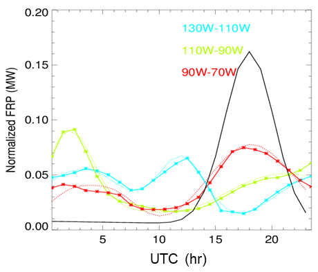
Figure 2 The diurnal cycle functions (solid lines (green, blue, and red)) developed based on GOES-16 FRP data during the FIREX-AQ period. The original WRF-Chem diurnal cycle function is also shown (solid black line). The dashed lines (green, blue, and red) show the normalized FRP.

In retrospective mode, the model has the same configuration as the forecast mode except that fire detections are for the current day, and the NOAA National Center for Environmental Prediction (NCEP) Global Data Assimilation System (GDAS) (Wang and Lei, 2014) is used for initial and lateral boundary meteorological conditions, and RAQMS is used for initial and lateral boundary aerosol conditions. The modeling experiments consisted of two sets of simulations with different WRF-Chem versions. Set 1 included the WRF-Chem version with the default PREP-Chem v1.3 fire emissions estimates, the Freitas et al. (2007) plume-rise model described earlier in this section (referred to as the 3BEM version hereon), and the diurnal cycle function peaking at 18:00 Z. Set 2 included the version with FRP-based emissions estimates and plume-rise model (referred to as FRP version hereon). Both Set 1 and Set 2 runs use the same emission factors from Andreae and Merlet (2001) and Longo et al. (2009). The FRP-based updates are implemented following the High-Resolution Rapid Refresh Smoke (HRRR-Smoke) modeling system, which is a forecasting modeling system providing high-temporal- and high-spatial-resolution (3 km) smoke forecasts for the CONUS (using the VIIRS fire product) (described in the next section). We also developed new diurnal cycle functions (solid red, blue, and green curves in Fig. 2) by adapting the default analytical function (shown in black in Fig. 2) to match the mean diurnal GOES-16 FRP profiles within three different longitude bands over the FIREX-AQ period (August–September 2019). The default diurnal cycle function for biomass burning emissions in WRF-Chem is a Gaussian function peaking at 18:00 UTC (Freitas et al., 2011). The GOES-16 FRP measurements during the FIREX-AQ period (August–September 2019) were divided into three zones based on longitude (zone 1 (blue in Fig. 2): −130 to −110^∘ W; zone 2 (green in Fig. 2): −110 to −90^∘ W; zone 3 (red in Fig. 2): −90 to −70^∘ W), and the mean FRP diurnal profiles were constructed for each zone. The default diurnal cycle function used in WRF-Chem was iteratively adjusted to match the FRP profiles for each zone, resulting in three diurnal cycle functions. These diurnal functions were used in the FRP version.

2.2 HRRR-Smoke model

The High-Resolution Rapid Refresh Smoke (HRRR-Smoke) model is a 3-D forecasting model (https://rapidrefresh.noaa.gov/hrrr/HRRRsmoke/, last access: 4 August 2022), which is run at NOAA/NCEP. It uses a single smoke tracer to simulate smoke emissions and transport at a high spatial and temporal resolution to provide real-time smoke forecasts. The model domain spans the CONUS with a horizontal spatial resolution of 3 km and 50 vertical levels. HRRR-Smoke forecasts are initialized every hour using the HRRR meteorological analyses, with the forecast lead times varying between 18–48 h. HRRR-Smoke is a coupled model where the direct radiative effects of smoke feedback on the dynamics. The model uses fire location (latitude, longitude) and FRP measurements from four polar-orbiting satellites, two (Suomi-NPP and NOAA-20) for VIIRS (375 m resolution I-band Active Fire (AF) algorithm which is based on the Moderate Resolution Imaging Spectroradiometer (MODIS) Collection 6 retrieval; Giglio et al., 2016) and two (Terra and Aqua) for MODIS. It employs an FRP-based methodology to estimate fire smoke emissions and simulate plume rise in the model. Smoke emissions in HRRR-Smoke are estimated by using FRP measurements to derive the fire radiative energy (FRE) over the fire duration (Ahmadov et al., 2017). The biomass burned is estimated by multiplying the FRE estimates with conversion coefficients from Kaiser et al. (2012). The model accounts for variation in these coefficients across ecosystems by using ecosystem-specific conversion coefficients. The land cover types in HRRR-Smoke are defined following the IGBP land cover classification (17 land cover types). The plume rise in the model is based on Freitas et al. (2007) with heat energy flux estimation parameterized as a function of FRP per unit fire size. HRRR-Smoke forecasts and simulations have been comprehensively evaluated for several fire seasons. These evaluations have included comparisons with hourly PM_2.5 measurements from the U.S. EPA Air Quality System Network at multiple sites in Washington state during the 2015 fire season (Deanes et al., 2016). The HRRR-Smoke model forecasts for FIREX-AQ were evaluated by Ye et al. (2021) using aircraft in situ and remote sensing measurements.

3 Data

3.1 GOES-16 fire product

GOES-16/GOES-East was the first in NOAA's GOES-R series of geostationary satellites. It was launched in November 2016 and occupies an orbit over 75.2^∘ W. The Advanced Baseline Imager (ABI) is a 16-channel (2 visible, 4 near-infrared, 10 infrared) passive imaging radiometer on board GOES-16. It provides imagery of the Earth's surface and the atmosphere at very high spatial (2 km for infrared bands) and temporal (5 min for CONUS, 15 min for the western hemisphere/full-disk) resolutions and includes several features that can be used to improve fire detection and emissions estimation. For example, the finer spatial and temporal resolution of ABI data would enable detection of small and short-lived fires. Under clear-sky conditions, the minimum detectable size of a fire (mean temperature: 800 K) is estimated to be 0.004 km² at the sub-satellite point. Short-lived fires are often missed by polar-orbiting satellites due to their limited temporal coverage.

The Fire Detection and Characterization (FDC) product is one of the multiple GOES-16 ABI-derived baseline products. The product has a spatial resolution of 2 km and is available for CONUS every 5 min. It uses a modified version of the Wildfire Automated Biomass Burning Algorithm (WF-ABBA) (Prins and Menzel, 1992, 1994; Prins et al., 1998, 2001; Schmidt and Prins, 2003) developed specifically for the ABI (referred to as ABI algorithm hereon). The ABI algorithm primarily relies on retrievals in the 3.9 and 11.2 µm spectral bands (ABI channels 7 and 14) and channel 2 (if available during daytime) to identify fires and derive sub-pixel fire properties in a two-step process consisting of identifying potential fires and subsequently filtering out false alarms. The algorithm uses several ABI (brightness temperatures/radiances (Channels 7 and 14 required, Channels 2 and 15 are optional), solar geometry, and ABI sensor quality 3BEM flags) and non-ABI datasets (global land cover classification, land–sea–desert mask from MODIS 5 collection, NCEP total precipitable water, MODIS global emissivity) in the process of deriving the final fire product. The product provides fire detection locations (latitude, longitude), fire properties (e.g., sub-pixel instantaneous fire size, fire radiative power, fire brightness temperature), and a metadata mask classifying each detection into one of six categories:

1. Code 10(30): processed fire (sub-pixel fire size and temperature estimated),

2. Code 11(31): saturated fire pixel,

3. Code 12(32): cloud contaminated (partially cloudy/smoke),

4. Code 13(33): high-probability fire,

5. Code 14(34): medium-probability fire, and

6. Code 15(35): low-probability fire.

The codes in parentheses are used when the detection also passes a temporal filtering test. We only use Codes 10(30) in this study due to the availability of both FRP and fire size estimates. The sub-pixel instantaneous fire size and temperature are estimated using the Dozier technique (Dozier, 1981). The Dozier method utilizes the total radiances in the 3.9 and 11.2 µm spectral bands and the respective radiances in these bands from the fire and the background to solve for the proportion of each ABI pixel that is on fire. Under realistic conditions (likely to be encountered in an operational environment), Giglio and Kendall (2001) estimated that the random errors (at 1 standard deviation) in estimating the fire size could be within 50 % when the proportion of the pixel on fire is more than 0.005. For proportions lower than 0.005, both the systematic and random errors could be greater. GOES-16 data for the FIREX-AQ campaign period were available publicly (FIREXAQ Satellite_data, 2021).

3.2 NASA DC-8 airborne observations from FIREX-AQ

3.2.1 Black carbon measurements from the NOAA Single-Particle Soot Photometer (SP2)

We use refractory black carbon (rBC) measurements (FIREXAQ Aerosol_AircraftInSitu_DC8_Data, 2020) from the NOAA Single Particle Soot Photometer (SP2) (Schwarz et al., 2006, 2008, 2010a, 2017; Perring et al., 2017) to evaluate WRF-Chem-simulated BC. Henceforth, we use the terminology BC to refer to both the material quantified by the SP2 and the modeled species. The SP2 is primarily used to measure the refractory black carbon (rBC) mass content of individual accumulation mode aerosol particles. These mass estimates are independent of the particle mixing state or morphology. The instrument has been used on various research aircraft to provide airborne rBC in situ measurements in multiple field campaigns (e.g., NASA DC-8 (SEAC4RS), Perring et al., 2017, NSF/NCAR GV (HIPPO), Schwarz et al., 2010b). The SP2 flew on board the NASA DC-8 for both the Boise and Salina phases of the FIREX-AQ field campaign and provided in situ measurements of rBC mass concentration (ng-BC/std. m³, 1013 mb pressure and 273 K temperature) at 1 Hz frequency. The rBC concentrations reported by the SP2 include final calibrations and adjustments for dilutions, a correction factor to account for the non-detected rBC (sizes outside of SP2 detection range, 90–550 nm) as well as rejection of highly contaminated (due to high concentrations) observations. Smaller concentration biases also occurring under high aerosol loadings (Schwarz et al., 2022) but affecting rBC concentrations by less than 20 % have not been corrected. Total uncertainty in accumulation mode rBC concentrations measured by the SP2 are less than or equal to 40 % in FIREX-AQ. As GOCART does not resolve BC aerosol size, and most biomass burning (BB) emissions occur in this size range, measurement bias relative to the model is negligible in the context of the order of magnitude shifts arising from emissions treatments explored here.

3.2.2 Organic aerosol measurements from the University of Colorado Boulder Aircraft High-Resolution Time-of-Flight Aerosol Mass Spectrometer

We use OA mass concentration measurements from the University of Colorado Boulder Aircraft High-Resolution Time-of-Flight Aerosol Mass Spectrometer (CU HR-ToF-AMS) (FIREXAQ Aerosol_AircraftInSitu_DC8_Data, 2020) and use the provided $\mathrm{OA}/\mathrm{OC}$ ratio (based on Aiken et al., 2008; Canagaratna et al., 2015) to derive OC concentrations for comparison to the WRF-Chem-simulated OC concentrations (note: $\mathrm{OA}/\mathrm{OC}$ is not computed for OA values under the detection limit, and for those data points a value of 1.8 $\mathrm{OA}/\mathrm{OC}$ was used, consistent with the GOCART assumptions). The CU HR-ToF-AMS (DeCarlo et al., 2006) can be used to perform high-temporal-resolution (demonstrated ability of measurements at 0.1 s; Guo et al., 2021) measurements of bulk organic aerosol with extensive characterization of its intensive properties (e.g., $\mathrm{O}/\mathrm{C}$, $\mathrm{H}/\mathrm{C}$, positive matrix factorization (PMF) factors) and inorganic salts (e.g., ammonium sulfate ((NH₄)₂SO₄), nitrate (NH₄NO₃), and chloride (NH₄Cl)) in the submicron range (up to 900 nm in vacuum aerodynamic diameter, Guo et al., 2021). It is one of the several available versions of the AMS that incorporates an improved high-resolution mass spectrometer. The instrument takes in ambient air through a dedicated aerosol inlet (HIMIL, Stith et al., 2009) into an aerodynamic lens (residence time < 0.4 s), which directs the particles into a narrow beam. The non-refractory particles are subsequently vaporized by impaction on a heated surface (600 ^∘C), and the vapors are ionized by electron ionization. Finally, these ions are analyzed by mass spectrometry. The CU HR-ToF-AMS flew on board the NASA DC-8 for both the Boise and Salina phases of the FIREX-AQ field campaign. The instrument provided in situ measurements at 1 Hz frequency and switched to a higher time resolution of 5 Hz to sample fire plumes, especially the smaller ones in the Salina phase.

AMS organic carbon (OC) is estimated from the total OA mass concentration and $\mathrm{OA}/\mathrm{OC}$ mass ratio measurements. $\mathrm{OA}/\mathrm{OC}$ is derived from carefully fitting all the organic peaks in the mass spectrum and applying a calibration (Aiken et al., 2008). The uncertainty (2σ) in OA is estimated as 38 % (Bahreini et al., 2009), based on the uncertainty in the relative ionization efficiency (Jimenez et al., 2016; Xu et al., 2018) and AMS collection efficiency (Middlebrook et al., 2012). This uncertainty was shown to be consistent with AMS measurements of aged particles (Guo et al., 2021). $\mathrm{OA}/\mathrm{OC}$ is estimated using two approaches: the “improved Aitken ambient” calibration for OA concentrations under 150 µg sm⁻³ and the “Aitken semi-explicit method” for OA concentrations higher than this (so most of the plume data in this study), as described in Canagaratna et al. (2015). Based on that analysis, for complex mixtures the uncertainty in $\mathrm{OA}/\mathrm{OC}$ is estimated at 8 % (2σ). Hence the total estimated uncertainty for OC is 39 %.

3.2.3 Aerosol optical property measurements from the NASA Langley Airborne high-spectral-resolution lidar (HSRL)

We use backscatter coefficient (532 nm) measurements from the NASA Langley airborne high-spectral-resolution lidar (HSRL) (FIREXAQ HSRL_AircraftRemoteSensing_DC8_Data, 2020; Hair et al., 2008) to compare to the WRF-Chem-simulated backscatter coefficient. The WRF-Chem backscatter coefficient is computed using the ratio of the WRF-Chem-simulated aerosol extinction coefficient for different species (BC+OC, SO${}_{\mathrm{4}}^{\mathrm{2}-}$, dust, SS) and the corresponding lidar ratios. The lidar ratios are used from Burton et al. (2012). The HSRL can provide measurements of aerosol backscatter and extinction coefficients (532 nm), aerosol backscatter coefficient (1064 nm), and aerosol depolarization (532 and 1064 nm). The instrument employs the HSRL technique at 532 nm and the standard backscatter lidar technique at 1064 nm. The HSRL technique relies on the differences in the spectral distributions of the backscattered lidar signal from aerosols and molecules. The returned lidar signal is split into two optical channels, namely the molecular backscatter channel and the total backscatter channel. The molecular backscatter channel consists of an iodine (I₂) vapor absorption filter, which removes the aerosol component of the returned lidar signal but passes the component due to molecules. The total backscatter channel is non-selective and allows all frequencies to pass. The uncertainties in the HSRL backscatter coefficient measurements (532 nm) can be mainly attributed to the iodine filter transmission measurements, calibration errors, molecular depolarization measurements, and atmospheric state variable measurements (Hair et al., 2008). The combined systematic error in the aerosol backscatter due to these factors is estimated to be less than 2.3 % (Hair et al., 2008).

4 Results and discussion

This section includes a discussion of the relevant FIREX-AQ flights, interpretation of the FIREX-AQ aerosol observations, and evaluation of the WRF-Chem model (3BEM and FRP versions) using FIREX-AQ observations of BC and OC backscatter. It also includes comparisons of simulated WRF-Chem AOD with observed AOD from GOES-16/17 and simulated plume heights with observed plume heights from the HSRL data. Plume height estimates are computed using the HSRL backscatter measurements and WRF-Chem-simulated backscatter. Plume height is defined as the height at which the maximum change in the magnitude of the backscatter gradient is observed. We only focus on FIREX-AQ DC-8 science flights during 3–7 August 2019. We do not include the flight on 8 August 2019 in the analysis since the primary focus of this flight was on the pyro-cumulonimbus cloud (pyro-Cb) produced by Williams Flats, and current computational models do not have the capability to simulate these events. The WRF-Chem plume rise (in both 3BEM and FRP version) is a 1-D cloud model with a simplified microphysics scheme without any coupling between heat fluxes generated from fires and meteorology. Therefore, simulation of pyro-Cb events is beyond the capability of current computational models. Ye et al. (2021) also reported the current inability of models to simulate pyro-Cb events based on their analyses of multiple forecasting models. However, recent work has focused on conceptual models that describe pyro-Cb (e.g., Peterson et al., 2017) development during wildfire events. These models could serve as a starting point towards incorporating pyro-Cb simulation capabilities in current computational models. We first provide an overview of the Williams Flats fire (Sect. 4.1), followed by brief descriptions of each FIREX-AQ DC-8 science flight (Sect. 4.2). The subsequent sections provide an evaluation of the WRF-Chem-simulated aerosol optical properties and $\mathrm{BC}/\mathrm{OC}$ concentrations during each of the FIREX-AQ DC-8 science flights. All altitudes reported are with respect to mean sea level (m.s.l.). We use the aircraft pressure altitude to represent the aircraft altitude. The WRF-Chem planetary boundary layer (PBL) height was converted to the mean sea level reference by adding the surface height to the WRF-Chem PBL variable.

4.1 The Williams Flats fire

The Williams Flats wildfire began on 2 August 2019 8 km southeast of Keller (southwestern Ferry County) in Washington (WA) USA. The fire was caused by lightning strikes accompanying an early morning thunderstorm near the Colville Indian Reservation. The 100 % containment date for the fire was reported to be 25 August 2019, and it burned an estimated 180 km² (https://data.statesmanjournal.com/fires/incident/6493/williams-flats-fire/, last access: 4 August 2022). The fire was the flagship fire of the Boise phase of the FIREX-AQ campaign and the focus of the DC8 science flights on 3, 6, 7, and 8 August 2019. These flights sampled both fresh and aged smoke plumes from the fire. On 8 August 2019, the fire also generated a pyro-Cb, which was sampled by the DC8 science flight for the day. The DC-8 science flight on 6 August also focused on the Horsefly fire. The Horsefly fire started on 5 August 2019 24 km east of Lincoln in Lewis and Clark County (Montana) and burned 5 km² in the first 24 h (https://data.redding.com/fires/incident/6502/horsefly-fire/, last access: 4 August 2022). The fire was reported to have burned 5 km² till 23 August 2019, with zero growth reported in the prior week (https://data.redding.com/fires/incident/6502/horsefly-fire/  last access: 4 August 2022).

4.2 The FIREX-AQ DC-8 science flights (3–7 August 2019)

4.2.1 3 August 2019 flight

The FIREX-AQ DC-8 science flight on 3 August 2019 involved extensive sampling of the Williams Flats fire and a high-altitude remnant of smoke associated with long-range transport. Figure 3a shows the flight track along with the WRF-Chem-simulated PBL. This science flight started with the DC-8 flying over the Lick–Mica Creek fire on the way from Boise to Williams Flats (∼ between 21:00 and 21:30 Z). The overall flight could be divided into two phases. Phase 1 (22:00–00:00 Z) was carried out at altitudes ranging from 2.7–3 km with sampling of the smoke plume extending 120 km downwind of the fire in the northeast direction. Between 21:30 and 22:00 Z, the aircraft traveled across Williams Flats to begin phase 1 of sampling. Phase 2 (∼ 00:30–02:30 Z) extended 65 km downwind of the fire, initially in the northeast direction and later in the eastern direction. The altitudes of sampling ranged between 3–3.4 km. Phase 2 began following a transit (between 00:00 and 01:00 Z) to the fire after phase 1.

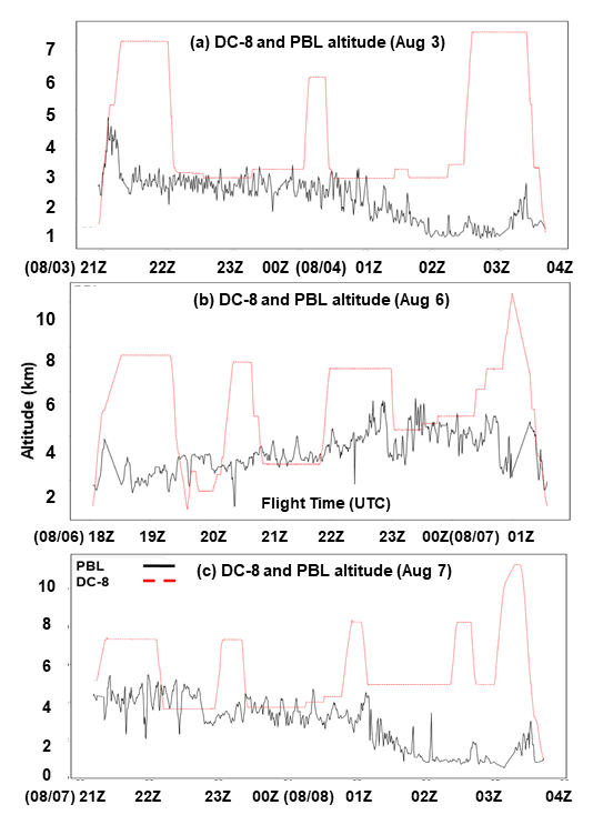
Figure 3 The DC-8 flight altitude (red) and the WRF-Chem planetary boundary layer height (black) for the 3 August 2019 (a), 6 August 2019 (b), and 7 August 2019 (c) flights.

4.2.2 6 August 2019 flight

The FIREX-AQ DC-8 science flight for 6 August 2019 had two targets, namely Williams Flats and the Horsefly fire in Montana (Fig. 3b). Williams Flats was sampled first followed by an extensive sampling of Horsefly, which spanned more than 200 km downwind of the fire. For Williams Flats, the sampling could be divided into two phases, with phase 1 focusing on sampling low-elevation smoke and phase 2 involving sampling of the fire plume at a higher altitude (∼ 3 km). Between 22:00–23:00 Z, the DC-8 traveled from Williams Flats towards Montana to sample the Horsefly fire and flew over the Snow Creek fire and Horsefly before beginning the sampling. For the Horsefly fire, the DC-8 traveled downwind in the plume starting at ∼ 23:00 Z and continuing sometime after 00:00 Z, which was followed by an upwind pass and return to Boise.

4.2.3 7 August 2019 flight

The 7 August 2019 FIREX-AQ DC-8 science flight (Fig. 3c) focused exclusively on the Williams Flats fire with a four-phase sampling strategy. Phase 1 involved sampling aged (transport age: 1 d old) smoke from the fire that was transported eastward to Montana. This smoke was sampled in both the east and west directions traveling along the axis of the plume. The remaining phases focused on fresh smoke from the fire, with phase 2 involving sampling at low altitudes (∼ 3.7–4.3 km) and phases 3 and 4 involved higher-altitude (∼ 4.9 km) sampling.

4.3 BC and OC emission estimates

Figure 4 shows the estimated BC and OC emissions (3BEM and FRP versions) for the Williams Flats fire on the DC-8 flight days (3–8 August 2019). Emissions from the Horsefly fire which was sampled on the 6 August flight are also shown. In general, the BC and OC emissions estimates from the FRP approach were significantly higher than the 3BEM approach on all flight days for the Williams Flats fire. For BC, the FRP-based emissions were 32 times higher on 3 August, when Williams Flats was in its initial stages and varied between 12 and 47 times the emissions in the 3BEM version till 8 August.

Figure 4 Model-predicted BC (a) and OC (b) emissions from the Williams Flats (WF) fire on the DC-8 science flight days (3–8 August 2019) during FIREX-AQ. The emissions for Horsefly (H) fire on 6 August 2019 are also included (bar set 3 for BC and OC).

OC emissions also showed a similar trend, with the FRP version emissions being 33 times higher on 3 August and 12–52 times higher for the remaining flight days. BC and OC emissions for both approaches increased from 3–8 August, with the maximum emissions observed on 8 August, when Williams Flats generated a pyro-Cb event. The Williams Flats fire increased significantly in size from 3–8 August (Ye et al., 2021), which is reflected in the increase in BC and OC emissions. Emissions in the 3BEM version were lower for the Horsefly fire as well, with the FRP-based emissions being 198 times higher for BC and 200 times higher for OC. Thus, the FRP-based approach yielded substantially higher emissions from wildfires as compared to the 3BEM approach. The significant differences in emissions in the two approaches could be attributed to the fundamental difference in the emissions estimation methodology in the two approaches. The 3BEM approach uses the instantaneous fire size while the HRRR-Smoke approach uses the FRP. Both these parameters could vary at substantially different rates over the lifetime of a fire and therefore could lead to very different results. Ye et al. (2021) compared the emissions between 12 different forecasting systems including WRF-Chem at UW Madison (using GOES-15 fire product) and HRRR-Smoke and found that models using FRP-based emission estimation approaches had substantially (mean factor of 5.6) higher emissions than those using burned-area-based (referred to as hotspot-based in their study) approaches.

We used the same emission factors in both the 3BEM and FRP versions to ensure that the changes in emissions solely represent the differences in the two methodologies. Considerable progress has been made in improving upon the emission factor estimates used in this study. For example, subsequent work by Akagi et al. (2011) (referred to as AK11), and Andreae (2019) (referred to as AN19) has resulted in new emission factor estimates for biomass burning. In comparison to these studies, our OC emission factors for tropical forests were 9 % higher than AK11 (BC: 21 %) and 15 % higher than AN19 (BC: 23 %) while for extratropical forests the emission factors were the same as AK11. AN19 did not report emission factors for extratropical forests. For savanna/grasslands, OC emission factors were 18 % higher than AK11 (BC: 20 %) and 6 % higher than AN19 (BC: 15 %). Thus, incorporation of these emission factors could alter the magnitude of emission estimates (for both 3BEM and FRP versions) reported in Fig. 4.

4.4 Simulated aerosol (BC and OC) concentrations during the Williams Flats fire

Figures 5 and 6 show the time series of in situ measurements of BC (SP2) and OC (AMS) and the WRF-Chem-simulated BC and OC (3BEM and FRP) along the DC-8 flight track for the DC-8 science flights. For the 3 August flight, the 3BEM version was up to a factor of 100 lower than the in situ BC measurements in phase 1 of sampling and up to ∼ 250 times lower in phase 2 (Fig. 5a). For OC (Fig. 6a), the 3BEM version underestimated the measurements by up to a factor of ∼ 125 in phase 1 and up to a factor of more than 300 in phase 2. Similar results were obtained for the other flights as well, where the 3BEM version was biased low for most of the 6 August flight with the simulated BC up to 440 times lower than the measurements (Fig. 5c) and OC up to 1065 times lower (Fig. 6c). For the 7 August flight, the 3BEM version was not able to reproduce the observed BC (Fig. 5e) and OC concentrations (Fig. 6e) during any of the sampling phases. The underestimations were up to a factor of 842 for BC and up to a factor of 1439 for OC. These results can be attributed mainly to the low emissions in the 3BEM version. The greater underestimation in phase 2 for BC and OC (3 August flight) and phases 3 and 4 of the 7 August flight could be due to the diurnal cycle imposed on the emissions resulting in lower emissions during these stages of the respective flights.

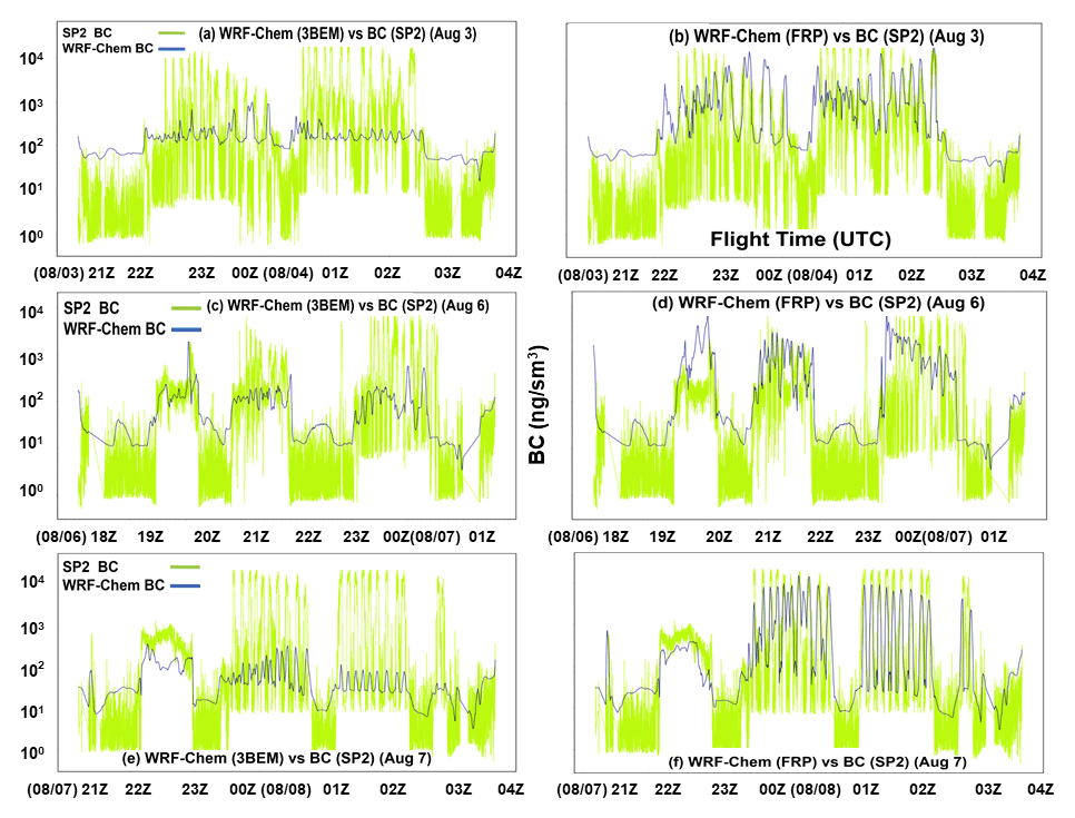
Figure 5 Time series for BC (SP2) in situ measurements and corresponding WRF-Chem-simulated BC (3BEM and FRP versions) for the 3 August (a, b), 6 August (c, d), and 7 August (e, f) DC-8 science flights.

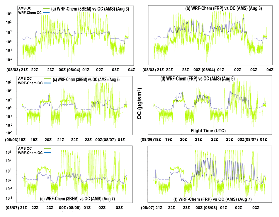
Figure 6 Time series for OC (AMS) in situ measurements and corresponding WRF-Chem-simulated BC (3BEM and FRP versions) for the 3 August (a, b), 6 August (c, d), and 7 August (e, f) DC-8 science flights.

The higher emissions in the FRP version result in better agreement with the SP2 and AMS in situ measurements throughout the flight periods. During the 3 August flight, the FRP version was able to reproduce the BC and OC enhancements observed near the fire and downwind well, with the simulated BC being up to a factor of ∼ 91 higher than the 3BEM version (Fig. 5b), while for OC (Fig. 6b), the FRP version was up to ∼ 28 times higher. Thus, the FRP version showed a significant reduction in discrepancies between WRF-Chem and the SP2/AMS in situ measurements. During the 6 August flight as well, the FRP version showed very good agreement for phase 2 of the Williams Flats sampling, where it was able to simulate concentrations of BC and OC comparable to the observations (Figs. 5d, 6d). For the Horsefly fire as well, the FRP version was able to simulate the high BC levels observed (Fig. 5d, 23:00 Z onward) but significantly underestimated OC (Fig. 6d, 23:00 Z onward). The FRP version simulated up to 125 times higher BC concentrations and up to 49 times higher OC concentrations than the 3BEM version. The 3BEM version was biased very low for BC and OC during phase 2 of Williams Flats and the Horsefly sampling. The BC and OC concentrations in the FRP version (Figs. 5d, 6d, 23:00 Z onward) declined sharply as the DC-8 flew downwind of Horsefly, which could be attributed to an underestimation of the injection heights or inability of the model to accurately simulate the transport of the plume downwind, resulting in lower plume heights than observed. The Horsefly fire plume altitude increased downwind as shown in the HSRL backscatter measurements (Fig. 9d, 23:00 Z onward). This was accompanied by a gradual ascent of the DC-8 aircraft as it tracked the fire plume (Fig. 9d). Since the plume height was very low in the model, the BC and OC concentrations along the flight track represented background level concentrations instead of the enhanced levels caused by the fire. These concentrations declined even further as the aircraft ascended in the later stages, which is observed in the time series during the Horsefly downwind sampling phase. However, the FRP version performed poorly as compared to the 3BEM version in simulating the low-elevation smoke as the FRP version significantly overestimated the BC and OC concentrations (Figs. 5d, 6d, 19:00–20:00 Z). During the 7 August flight as well, the FRP version was able to reproduce the observations very well, especially in the fresh smoke sampling phases of the flight. The higher emissions in the FRP version resulted in BC concentrations up to 124 times higher and OC concentrations up to 78 times higher than the 3BEM version (Figs. 5e, f and 6e, f). Both the 3BEM and FRP versions underestimated the aged smoke, which could be due to simplified chemistry in the GOCART mechanism. The underestimation of OC in the model was larger than BC, which could also be a consequence of the simplified chemistry in the model.

4.5 Simulated aerosol optical properties during Williams Flats

4.5.1 Aerosol optical depth (AOD)

Figure 7 shows the WRF-Chem-simulated AOD (3BEM and FRP versions) for the Williams Flats fire during the 3 August (a–d), 6 August (e–h), and 7 August (i–l) DC-8 science flights. The DC-8 flight track during the different phases of each flight is overlaid. The 3BEM version simulated substantially low AOD enhancements during all the science flights as compared to the FRP version. During the 3 August flight (Fig. 7a, c), minor AOD enhancements (∼ 0.3–0.6) were simulated due to the Williams Flats fire. AOD enhancements were higher in the vicinity of the fire during phase 1 of sampling (Fig. 7a, 00:00 Z) but dissipated during the latter stages of the flight (Fig. 7c, 04:00 Z, AOD: 0–0.2). For the remaining flights as well, the simulated AOD enhancements were very low (6 August (0.0–0.3) and 7 August (0.2–0.6)) as compared to those in the FRP-based version. The simulated plumes for the Williams Flats and Horsefly fires during the 6 August flight were either thin or not noticeable, while for the 7 August flight, the AOD enhancements (0.2–0.6) were prominent only during the early stages of the flight and further declined during the fresh smoke sampling phase. The plume from the Williams Flats fire was only evident during the early stages of the flight and was characterized by very low aerosol loadings. In contrast, on 3 August, the FRP version simulated significantly higher AOD enhancements both near the fire and in the transported plume downwind. These enhancements persisted throughout the DC-8 sampling period at 00:00 and 04:00 Z. On 6 August, the FRP version simulated well-defined plumes with higher AOD (0.3–> = 1.0) for both Williams Flats and Horsefly. The spatial location and extent of the plumes were in good agreement with the DC-8 sampling legs, with the Horsefly fire plume being represented very well by this version (Fig. 7h) based on the DC-8 sampling pattern. Similar agreement was observed for the plume from Williams Flats, which was predominantly towards the east. Similar results were obtained for the 7 August flight, with very high AOD enhancements (> = 1) near the fire both before and during the fresh smoke sampling phase, and a well-defined and persistent plume throughout the DC-8 sampling period coincided well with the DC-8 flight path during the fresh smoke sampling phases. The aged smoke plume from Williams Flats in Montana did not appear as a distinct feature in the WRF-Chem AOD plots for both versions, which could possibly be due to the low simulated aerosol concentrations. The lower AOD simulated by the 3BEM version is primarily due to the lower emissions (Sect. 4.3) in comparison to the FRP version while the decline in AOD during phase 2 (3 August flight) could be due to the imposed diurnal cycle on emissions (maxima at 18:00 Z) in this version. The 3BEM version simulated the plume formation and downwind transport of smoke towards the northeast during phase 1, but the decline in emissions in phase 2 resulted in a non-discernible plume with very low AOD enhancements. In comparison, the FRP version simulated a far more intense plume with AOD enhancements greater than or equal to 1 near the fire and in the east-southwest direction. The plume coincided well with the sampling trajectory of the DC-8, indicating that the model simulated the spatial extent of the plume reasonably well. The estimated emissions for Williams Flats were lower for 6 August as compared to the other flight days, which resulted in the relatively lower AOD enhancements than those on 3 August.

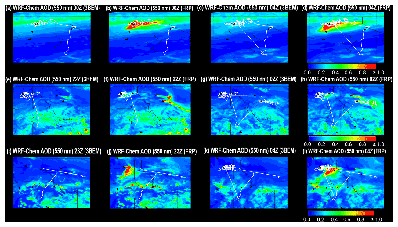
Figure 7 WRF-Chem-simulated aerosol optical depth (AOD) for the 3BEM and FRP versions during the FIREX-AQ DC-8 science flights on 3 August (a–d), 6 August (e–h), and 7 August (i–l). The DC-8 flight track is overlaid. The triangle markers indicate the locations of active fires.

Figure 8 shows comparisons of AOD available from the GOES-16/17 ABI AOD product (Gupta et al., 2019) with the simulated WRF-Chem AOD (3BEM and FRP versions) for all the DC-8 science flights. AOD computed from the HSRL backscatter is also included. The HSRL AOD was computed by multiplying the HSRL backscatter with the lidar ratio for $\mathrm{BC}/\mathrm{OC}$ to estimate the extinction coefficient and subsequently integrating the extinction coefficient. We only carry out these comparisons for the Williams Flats fire in the spatial domains shown in Fig. 8a–c. The domains were chosen to include the fire as well as the region impacted by the fire plume and sampled by the DC-8 during the respective science flights. We only consider the time periods relevant to the DC-8 sampling of the Williams Flats fire (3 August: 22:00–2:30:00 Z, 6 August: 19:30:00–22:00 Z, 7 August: 23:00–2:30:00 Z). In general, the GOES-16 AOD product had a low bias as compared to the GOES-17 AOD product in both the median (GOES-16: 0.26–0.29, GOES-17: 0.33–0.45) and extreme values, which could be due to the differences in availability of data from the two satellites during the time period considered. The HSRL AOD (median: 0.32–2) was the highest amongst all the data sources (except 6 August) and exhibited the most variability as well, reflecting the fine temporal and spatial resolution of the HSRL measurements. The significant underestimation of aerosol concentrations in the 3BEM version is evident here as well, with the simulated median AOD values (0.07–0.24) and the extreme values being lower than those from the other data sources. This further indicates the inability of this version to capture the AOD enhancements observed near the fire and in the associated plume. The underestimation as compared to the FRP version (median: 0.24–0.78) has already been demonstrated and will not be discussed further. The AOD enhancements close to the Williams Flats fire were overestimated by the FRP version on 3 and 7 August (e.g., outlier values) as compared to GOES-16/17 estimates, while on 6 August this version was biased low due to underestimation of emissions. The agreement on 3 August and 7 August tended to be better farther away from the fire (e.g., downwind plume), resulting in closer median AOD values for the FRP version (3 August: 0.78, 7 August: 0.43) as compared to GOES-16/17 (GOES-16: 3 August: 0.26, 7 August: 0.29; GOES-17: 3 August: 0.33, 7 August: 0.40). On the other hand, comparisons with HSRL_AOD present an opposite picture with significant underestimation by the FRP version on 6 and 7 August both near and far away from the fire.

Figure 8 AOD estimates for HSRL, GOES-16/17, and WRF-Chem (3BEM and FRP versions) for the 3 August (d), 6 August (e), and 7 August (f) DC-8 science flights. The domain over which the AODs are being compared is also shown (a–c). Each box plot represents the minimum value, lower quartile, median, upper quartile, and maximum value. The mean is represented as the asterisk (^*) symbol in the bar, and the outliers are represented by the star symbols.

Potential caveats in these comparisons include the availability of GOES-16/17 data during the entire time period considered. There could be cases where data during the highest AOD periods are not available due to factors such as cloud cover. In addition, the procedure of computation of aerosol optical properties in WRF-Chem could impact the computed AOD values (discussed later in Sect. 4.6). Furthermore, the HSRL AOD is derived from the backscatter using literature lidar ratio values rather than direct integration of the extinction profile. Overall, the general conclusions that can be drawn from these comparisons are that the FRP version demonstrates the capability of simulating the high AOD values which accompany major wildfire events. However, it also has the tendency to overestimate the AOD when compared with the GOES-16/17 ABI AOD product.

4.5.2 Aerosol backscatter

Figure 9 shows the curtains for HSRL aerosol backscatter coefficient (referred to as backscatter hereon) measurements (a, d, g) and the simulated WRF-Chem backscatter (3BEM (b, e, h) and FRP (c, f, i) versions) for the 3–7 August DC-8 science flights. The DC-8 flight track is also shown. For the 3 August flight, the HSRL measurements (Fig. 9a) show the plume from the Lick–Mica Creek fire (∼ between 21:00:00 and 21:30:00 Z) reaching an altitude of ∼ 3 km. These enhancements were underestimated by both the 3BEM (Fig. 9b) and FRP (Fig. 9c) versions possibly due to an underestimation in emissions for this fire. The subsequent time periods in the HSRL observations represent the DC-8 sampling phases of Williams Flats. Between 21:30:00 and 22:00:00 Z, the aircraft traveled across Williams Flats to begin phase 1 of sampling. The phase 1 sampling period began just after 22:00 Z and continued downwind of the fire till 00:00 Z followed by a return transit to the fire (between 00:00 and 01:00 Z) and phase 2. The HSRL measurements show an alternating sequence of high and low backscatter enhancements during phases 1 and 2, which represent the aircraft traversing laterally in and out of the plume. The 3BEM version simulated localized backscatter enhancements near the fire during the early stages of phase 1 (22:00–23:00 Z). These enhancements were lower than the HSRL observations and declined significantly as the aircraft moved downwind (23:00–00:00 Z) consistent with the observations. The enhancements in the downwind plume were underestimated. In phase 2, the 3BEM version simulated backscatter enhancements lower than that in phase 1 near the fire (00:00–01:00 Z), which continued to decline as the aircraft moved downwind. The lower enhancements in phase 2 as compared to phase 1 are consistent with the declining phase of the emissions diurnal cycle in the 3BEM version. Thus, the 3BEM version showed several discrepancies with the HSRL measurements which included underestimation of backscatter near and downwind of the fire in both phases 1 and 2. The FRP version showed better overall agreement, with the HSRL measurements simulating comparable backscatter enhancements to the HSRL measurements during most parts of phases 1 and 2. The FRP version was also able to better capture the observed variation in the aerosol backscatter as the aircraft traversed in and out of the plume, although the coarse spatial resolution of the model (8 km × 8 km) acts as a limitation in exactly simulating the observed variation from the center to the edge of the plume. In phases 1 and 2, the model simulated continuously high aerosol backscatter near the fire, which was also observed by HSRL. It was also able to reproduce the variations in observed aerosol backscatter due to the closely spaced legs of the DC-8 flight near the fire and widely spaced legs of the DC-8 flight downwind of the fire in phase 1. For example, the alternate sequence of high–low aerosol backscatter is wider for the widely spaced legs of the flight (downwind of the fire) as compared to the closely spaced legs near the fire. The model was also able to reproduce the variation in backscatter observed downwind of the fire very well, especially in phase 1. Thus, the model simulated a plume with high aerosol loadings near and extending a significant distance from the fire, which was more consistent with the observed plume as is evident in the better agreement with the HSRL measurements. The FRP version appears to overestimate the plume height for several parts of the flight (e.g., either side of 22:00 Z, at 03:00 Z, phase 1 and transit phase before phase 2) but showed better agreement with the HSRL measurements in the latter part of phase 2 (after 01:00 Z) when the fire had intensified.

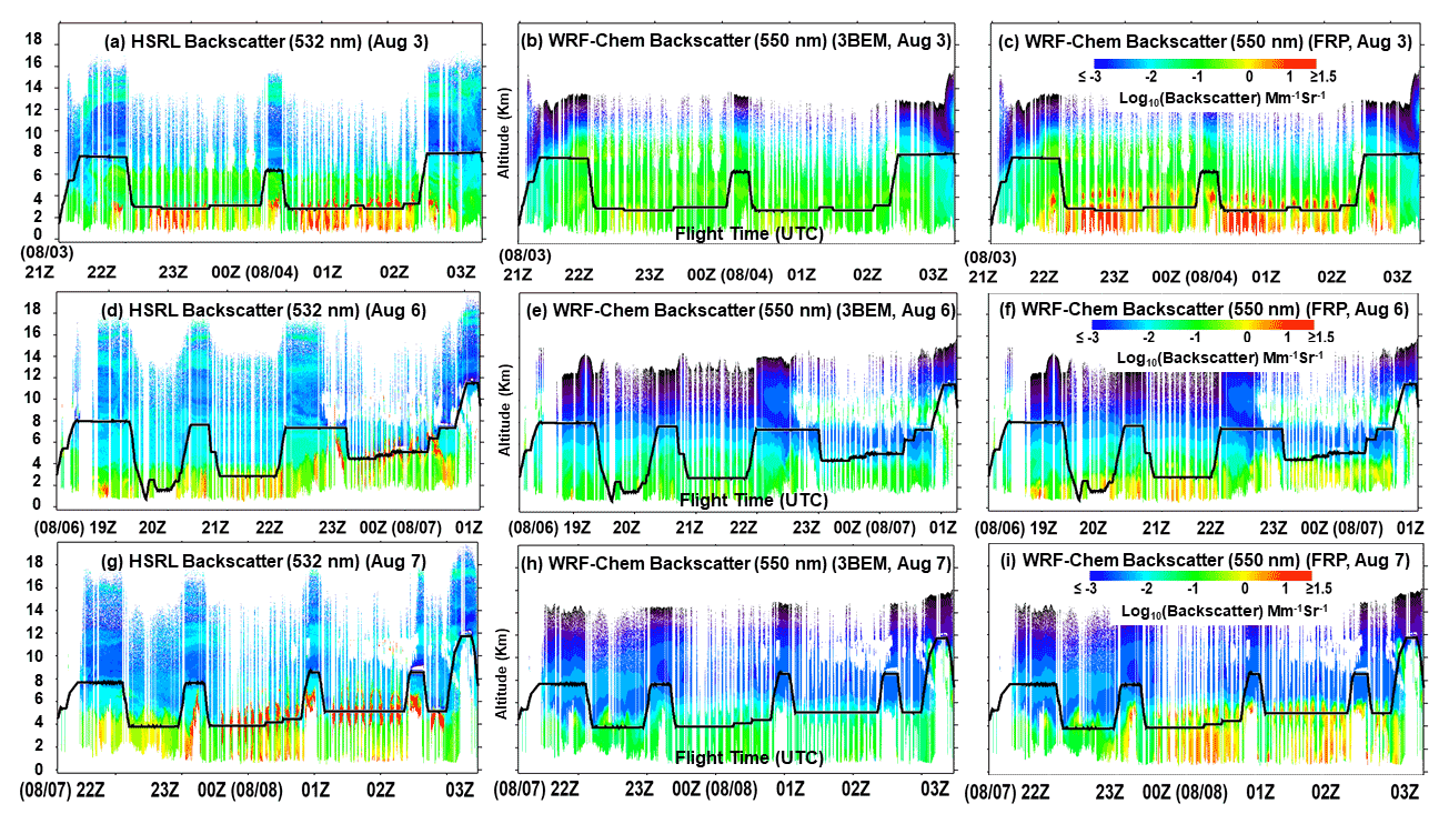
Figure 9 Flight curtains for the HSRL backscatter along with the WRF-Chem (3BEM and FRP versions) simulated backscatter (DC-8 science flights for 3 August a–c, 6 August d–f, and 7 August g–i).

Figure 9d–f represent the 6 August DC-8 sampling of the Williams Flats fire during phase 1 (between ∼ 19:30:00 and 20:00 Z) and phase 2 (21:00 to 22:00 Z) and the Horsefly fire from 23:00 Z to just before 00:30 Z. The backscatter enhancements during phase 1 (low-level smoke sampling) were underestimated by the WRF-Chem 3BEM version while the FRP version tended to overestimate. The HSRL measurements (Fig. 9d) were not available near 20:00 Z (below the DC-8) due to attenuation, which precludes any further comparisons. During 20:00–21:00 Z, the high backscatter in the HSRL measurements corresponds to Williams Flats as the DC-8 flew over the fire to begin phase 2 of sampling. These enhancements were largely absent in the 3BEM version (Fig. 9e) but were reproduced well in the FRP version (Fig. 9f). During phase 2 of sampling (21:00–22:00 Z), the 3BEM experiment only simulated sporadic backscatter enhancements, which were biased low as compared to the HSRL measurements. The measurements showed consistently high backscatter as the DC-8 traversed along the plume with the alternating bands of high–low backscatter again reflecting the periods the aircraft was within the plume or entering or leaving it. The FRP version did a better job than the 3BEM version, simulating comparable backscatter enhancements to the HSRL measurements and representing the variation along the flight track well. The HSRL backscatter enhancements between 22:00–23:00 Z were due to the Snow Creek and Horsefly fires and were better represented by the FRP version. For the Horsefly fire, the DC-8 traveled downwind in the plume starting at ∼ 23:00 Z and continuing sometime after 00:00 Z, which was followed by an upwind pass. The 3BEM version was biased low for this entire period consistent with the low emissions. The FRP version did simulate higher backscatter enhancements than the 3BEM version throughout this period, but it was unable to reproduce the peak enhancements in the HSRL measurements. In addition, WRF-Chem (3BEM and FRP) underestimated the plume height for Horsefly (< = 4 km) as compared to the HSRL observations (∼ 4–6 km). Consequently, the variation in the backscatter enhancements along the flight track does not agree with the HSRL observations.

Figure 9g–i show the HSRL backscatter measurements and WRF-Chem backscatter (3BEM and FRP runs) for the 7 August flight. The HSRL measurements (Fig. 9g) show the aerosol layer height due to the aged Williams Flats plume extending close to 6 km, which was simulated very well by both the 3BEM (Fig. 9h) and FRP runs (Fig. 9i), although both versions were biased low. The HSRL measurements showed very high aerosol backscatter during the period of fresh smoke sampling till ∼ 7 km. This was reproduced well by the WRF-Chem FRP version; however the altitude was underestimated (∼ 5.5–6 km), and for the 3BEM run, the backscatter enhancements were very low. During phase 2 of the sampling as the DC-8 moved along the plume, the HSRL measurements showed high aerosol backscatter values throughout with plume heights extending till ∼ 6 km. The 3BEM version failed to capture the observed enhancements and was biased low throughout the remainder of the flight mainly due to the low emissions. The FRP version consistently simulated significantly higher backscatter as compared to the 3BEM run and simulated the plume height between 5–6 km. The observed plume heights in phase 2 of the flight ranged from ∼ 5–6.5 km, and the backscatter levels were high as shown in the HSRL observations (01:00–02:00 Z). The FRP version simulated enhancements comparable to the HSRL observations but was still biased low. The vertical extents were ∼ 5–5.5 km, which was in reasonable agreement with HSRL measurements. The backscatter observed during the last pass over the fire at 8 km altitude was also well simulated by the FRP version, with a plume height of ∼ 5.8 km matching well with that observed in the HSRL data (∼ 6 km). During phase 4, the FRP version showed significantly better agreements with the HSRL observations, with higher enhancements than the 3BEM run and a predicted plume height of ∼ 5 km agreeing very well with the HSRL observations (∼ 5 km).

4.6 Statistical comparison of WRF-Chem and FIREX-AQ measurements

4.6.1 Distributions of aerosol concentrations, optical properties, and plume heights

Figure 10a–i show the comparison of frequency distributions of the FIREX-AQ measurements vs. WRF-Chem (3BEM and FRP runs) for BC and OC and the backscatter for the 3–7 August DC-8 science flights. The BC and OC distributions only account for the cases when the aircraft was in a smoke plume. The backscatter distributions are based on all observations during the flight period. For BC and OC, during the 3 August flight (Fig. 10a, d), the in situ measurements spanned a wide range (BC: 1 to > 10⁴ ng sm⁻³ and OC: ∼ 0.1 to ∼ 3000 ng sm⁻³), which reflects the contrasting aerosol concentrations in the environments in which the aircraft sampling occurred. For example, sampling included the center and edges of the Williams Flats plume both near and a significant distance downwind from the fire as well as remnants of any pollution at high altitudes. Aerosol concentrations in both cases could be very different considering that the flight sampled fresh Williams Flats smoke while the pollution remnants at high altitudes would have undergone significant dilution and thus would have much lower aerosol concentrations. WRF-Chem (3BEM and FRP versions) showed less variability in the simulated BC and OC concentrations than the measurements, which could be due to the coarse spatial resolution of the model and simplified chemical mechanism in the GOCART scheme. The 3BEM version captured very little of the observed variability in the BC and OC measurement distributions. It simulated BC concentrations most frequently between ∼ 80–250 ng sm⁻³ and OC concentrations between ∼ 4–10 ng sm⁻³, with a small fraction of higher values (BC: 250–900 ng sm⁻³, OC: 10–11 ng sm⁻³). The FRP version had an identical distribution for the lower end of concentrations (BC: 80–100 ng sm⁻³, OC: 4–6 ng sm⁻³), which is representative of the remote atmosphere and high altitudes where the impacts of changes in emissions and the plume rise are negligible. The FRP version was able to reproduce the observed distribution to a much better extent, especially for the high BC and OC concentrations (BC > 105 ng sm⁻³, OC > 80 ng sm⁻³) relevant for large wildfire events, reflecting the impacts of higher emissions. The high biases in both versions of the model for the frequency of lower-end concentrations (BC < 80 ng sm⁻³, OC < 3 ng sm⁻³) could correspond to the cases when the DC-8 was at the plume edge or when environments with low aerosol concentrations were being sampled (e.g., the long-range-transport plume). The model with its coarse spatial resolution (8 km × 8 km) could not accurately simulate the variability observed while transiting from the center of the plume to the edges. The observed distributions for BC and OC for the 6 August flight (Fig. 10b, e) represented a similar range of in-plume concentrations as the 3 August flight; however, the lower-end concentrations were higher for BC and OC, possibly due to this flight focusing only on fresh smoke sampling unlike the 3 August flight, which also sampled aged smoke (long-range-transport plume). The significant variance of the BC and OC distribution also reflects the various sampling conditions such as the aircraft traversing through the plume encountering high concentrations at the center and lower concentrations towards the edges, the different altitudes of sampling (phase 1 at lower altitude and phase 2 at higher altitude for Williams Flats), and traversing downwind from the Williams Flats and Horsefly fires. Similar to the 3 August flight, the WRF-Chem BC and OC distributions could not capture all the variability in the observations and were also biased high primarily due to the coarse model resolution, which precluded accurate simulation of the observed variability from the plume center to the edges. The 3BEM version distribution was able to better capture the variability in the BC and OC distributions than for the 3 August flight, which was mainly due to the better simulation of BC and OC concentrations in the low-altitude Williams Flats smoke. However, it still had a low bias compared to BC and OC measurements. The FRP version showed good agreement with the BC distribution, although it was biased low for OC. The low bias could primarily be attributed to the underestimation during the Horsefly sampling phase and the simplified chemistry in the GOCART mechanism (no SOA). Nevertheless, the distributions for the FRP version showed both an increase in variability and a shift towards higher simulated BC and OC concentrations. This resulted in better simulation of the variability in the BC and OC measurement distribution as compared to the 3BEM version and better agreement with the observed BC and OC distributions at concentration levels relevant for fire plumes. For the 7 August flight, the observed distributions for BC and OC (Fig. 10c, f) were similar to the previous flights, exhibiting high variability due to the sampling of a wide range of aerosol loading environments. For example, the Williams Flats aged plume was characterized by significantly lower aerosol concentrations as compared to the fresh plume sampled later. In addition, similar to the previous flights, the concentrations at the edge and center of the plume would also contribute to the variability observed in the BC and OC observation distributions. WRF-Chem (FRP version) was able to reproduce a significant fraction of this variability for BC and OC in particular for the high concentrations, as shown in corresponding distributions.

Figure 10 Frequency distributions for BC (a–c), OC (d–f), and backscatter coefficient (g–i) for the 3, 6, and 7 August DC-8 science flights. Note: BC and OC only represent in-plume cases.

The backscatter distributions were similar to the BC and OC distributions except that the model was closer to the measurements (e.g., 3 and 7 August flights; Fig. 10g, i) even though it was underestimating BC and OC. A potential reason for this discrepancy could be that we use lidar ratios from previous work in deriving the backscatter from the WRF-Chem aerosol extinction coefficient. In addition, meteorological parameters (e.g., relative humidity) and multiple aerosol species properties are used in computation of aerosol optical properties, which could result in biases in the estimation. For the 3 August flight, the backscatter distributions were identical for the 3BEM and FRP versions for low values (< 0.7 Mm⁻¹ Sr⁻¹). These values could represent the high-altitude phases of the flight during transition from Boise to Williams Flats where the effects due to fires would not be a factor. Similar to the BC and OC distributions, the FRP version captured the observed backscatter distribution well, especially for the higher values which were due to Williams Flats. The backscatter distribution derived from the HSRL measurements for the 6 August flight (Fig. 10h) showed similar characteristics, with lower values (< 0.01) primarily representing very high altitudes with no influence of fire emissions. This region was identically simulated by WRF-Chem (3BEM and FRP) since the primary differences between the two versions (fire emissions and plume rise) had little or no effect at these altitudes. The backscatter distribution also exhibited considerable variability (values spanned 6 orders of magnitude), which was consistent with the high variability observed in the BC and OC distributions. The backscatter distribution for the FRP version also showed a shift towards simulating higher enhancements than the 3BEM version and showing better agreement with the HSRL distribution at backscatter levels relevant to major fire events. The backscatter distribution of the FRP version also showed better agreement with the HSRL backscatter distribution. These major changes, which were also found in earlier flights, include a significant shift in the BC and OC backscatter distributions towards higher values and better agreement with observations.

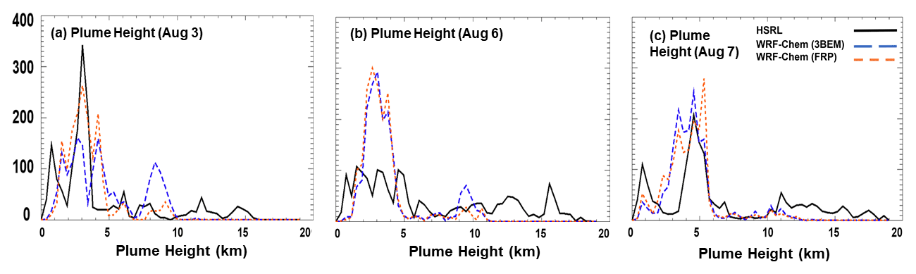
Figure 11 Frequency distributions for estimated plume heights for the 3 August (a), 6 August (b), and 7 August (c) DC-8 science flights.

Figure 11a–c show the estimated plume height distributions from the HSRL measurements along with the simulated plume heights from WRF-Chem (3BEM and FRP versions). For the 3 August flight (Fig. 11a), the best estimated plume heights based on HSRL observations were ∼ 3 km (represented by the highest peak in Fig. 11a) during the flight. In contrast, both 3BEM and FRP versions showed additional peaks in their distribution functions on either side of the observed peak. Therefore, the predicted plume heights varied between 2.7–4.1 km for the 3BEM version and 3–4.1 km for the FRP version. The FRP version did produce a better agreement with the observed plume heights based on the highest peak in the distribution function but also overestimated the heights for some parts of the flight. Moreover, the low-elevation smoke (represented by the peak < 1 km in HSRL) was either not captured or overestimated (peak ∼ 1.5 km) by both WRF-Chem versions. The plume height distribution (6 August flight, Fig. 11b) based on HSRL measurements showed several peaks, which could be attributed to the multiple altitudes at which smoke was sampled during this flight. Based on the observed peaks, the heights could have ranged from 0.75 to 6 km. The heights between 3–6 km are associated with the high-altitude Williams Flats plume and the Horsefly fire plume while the < 3 km altitude heights are from the lower-altitude Williams Flats smoke. Neither WRF-Chem version could capture this variability in the observed plume height distribution and simulated smoke heights of ∼ 3 km (peak 1) and ∼ 3.8 km (peak 2) for the 3BEM version (∼ 2.7 and ∼ 3.8 km for the FRP version). Thus, WRF-Chem underestimated the plume heights for this flight, which as discussed earlier in this section, could be a possible reason for the sharp decline in the simulated BC and OC concentrations as the DC-8 proceeded downwind of the Horsefly fire. For the 7 August flight, the estimated plume heights from HSRL showed one prominent peak near 5 km which would correspond to the Williams Flats smoke (aged and fresh). For the WRF-Chem 3BEM version, the simulated plume height varied between 3.5–5 km (based on the two peaks in the distribution), while the FRP version varied from 3.5–5.5 km. Thus, both versions showed significant variability in the plume heights, which could be due to different simulated injection heights in the model.

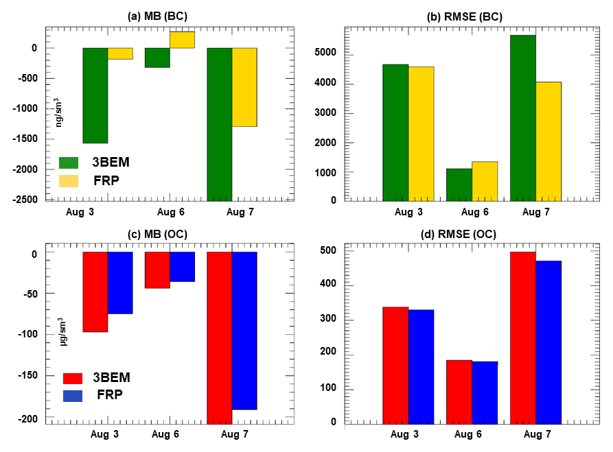
Figure 12 Statistical metrics of comparisons for BC and OC for the 3, 6, and 7 August DC-8 science flights. The average bias (MAB) and the root-mean-squared error (RMSE) for BC (a, b) and OC (c, d) are shown.

4.6.2 Statistical metrics for BC and OC comparisons

Figure 12 shows statistical metrics of comparisons between the WRF-Chem-simulated BC and OC and the SP2 and AMS observations for the respective species for all FIREX-AQ DC-8 flights considered in this work. The statistics reported are

$$\begin{array}{ll}\text{(1)}& {\displaystyle }& {\displaystyle }\text{mean bias (MB)}=\left({\displaystyle \frac{\mathrm{1}}{N}}\right)\sum _{i=\mathrm{1}}^N\left(X_{{\text{WRF-Chem}}_i}-X_{{\mathrm{Obs}}_i}\right),{\displaystyle }& {\displaystyle }\text{root-mean-squared error (RMSE)}=\\ \text{(2)}& {\displaystyle }& {\displaystyle }\sqrt{\left({\displaystyle \frac{\mathrm{1}}{N}}\right)\sum _{i=\mathrm{1}}^N{\left(X_{{\text{WRF-Chem}}_i}-X_{{\mathrm{Obs}}_i}\right)}^{\mathrm{2}}}.\end{array}$$

The 3BEM version had a low bias for both BC and OC, which was reduced significantly in the WRF-Chem FRP version. The MB and RMSE were reduced for the 3 August flight (MB: 88 % (BC) and 23 % (OC); RMSE: 2 % (BC) and 2.4 % (OC)) and 7 August flight (MB: 49 % (BC) and 9 % (OC); RMSE: 28 % (BC) and 5.2 % (OC)), which was primarily due to the better agreement of the simulated $\mathrm{BC}/\mathrm{OC}$ concentrations in the fresh smoke sampling phases of both flights. However, the model still underestimates $\mathrm{BC}/\mathrm{OC}$ as indicated by the negative MB values. The only exception was the 6 August flight, for which the performance of the FRP version degraded (only for BC) as compared to the 3BEM version. The MB and RMSE for BC increased primarily due to the significant overestimation of BC during the low-level smoke sampling period (Fig. 5d, 19:00–20:00 Z). The overestimation was larger for BC; therefore MB and RMSE were worse than those for OC. The significantly better model performance with the FRP version was partly offset by the inability of the model to simulate the aged part of the Williams Flats fire.

5 Conclusions

This study employs the Weather Research and Forecasting with Chemistry (WRF-Chem) model (retrospective simulations) with GOES-16 FRP-based methodologies to estimate wildfire emissions and simulate wildfire plume rise and diurnal cycles to interpret in situ and remote-sensing measurements collected aboard the NASA DC-8 aircraft during the 2019 NASA-NOAA FIREX-AQ field campaign and perform model evaluations. The primary focus is on the 3–7 August 2019 science flights that sampled the Williams Flats fire in Washington. The main conclusions from this evaluation are as follows.

1. The FIREX-AQ observations were characterized by a variety of aerosol loading environments, which resulted in a large range of $\mathrm{BC}/\mathrm{OC}$ and aerosol backscatter values during the 3–8 August science flights. These environments included fresh and aged smoke from Williams Flats and high-altitude remnants of a plume that could have undergone long-range transport. The altitudes of sampled smoke ranged from low altitude (6 August) to a pyro-Cb (8 August).

2. The GOES-16 FRP-based emissions employing the HRRR-Smoke methodology are substantially higher than the standard emissions inventory (Freitas et al., 2011) in WRF-Chem v3.5.1.

3. Wildfire emissions in the standard WRF-Chem (3BEM version) resulted in significant underestimation of carbonaceous aerosol (BC and OC) concentrations observed during the Williams Flats sampling flights in FIREX-AQ. The implementation of FRP-based emissions resulted in better agreement of model-simulated BC and OC concentrations when compared to in situ BC and OC measurements, thereby showing potential to improve the capability of WRF-Chem in simulating the high BC and OC enhancements observed during large wildfire events like the Williams Flats fire.

4. The simulated plume heights in the WRF-Chem FRP version did not show as large of changes as the emissions. The HRRR-Smoke FRP-based plume-rise methodology produced similar plume height distributions to the standard plume-rise approach included in WRF-Chem v3.5.1 (Freitas et al., 2007, 2010). Thus, the better performance of the WRF-Chem FRP version was mainly driven by the higher emissions in the FRP-based version.

5. The diurnal cycle imposed on wildfire emissions in WRF-Chem was also an important factor. For multiple flights, the standard WRF-Chem v3.5.1 with a diurnal cycle peaking at 18:00 UTC (Freitas et al., 2011) simulated declining emissions, AOD, and BC and OC concentrations during the latter stages of the science flights, while observations often showed increases during these periods. This shortcoming was not found in the FRP version, which employed new FRP-based diurnal cycle functions accounting for the variation with longitude.

6. WRF-Chem with the simplified GOCART mechanism could not adequately reproduce the aerosol concentrations in the aged smoke (1 d of more of aging). This was observed for all science flights that sampled aged smoke from Williams Flats. In addition to the primary factors such as emissions, plume height, and wildfire diurnal cycle estimation, second-order issues like biases in the aerosol dynamics (simulation of aerosol loss processes/transport) or chemistry (e.g., no SOA in GOCART) could play a role here. It would be worthwhile to evaluate these flights in the future with a more comprehensive chemistry mechanism (including SOA) to better understand the underlying causes.

Overall, the implementation of HRRR-Smoke FRP-based methodologies in WRF-Chem resulted in significantly better chemical forecasts for large wildfire events like the Williams Flats fire. Improvements in chemical forecasts could translate into better estimates of impacts of large wildfire events on human health, which is a cause of concern given the current and future trends in wildfire activity in the US. The comparisons between the 3BEM and HRRR-Smoke FRP-based emissions methodologies shown in this study also demonstrate that the HRRR-Smoke FRP-based emissions show the potential to improve the forecast capability during major fire events and would be useful to be incorporated in computational models providing air quality forecasts.