the Creative Commons Attribution 4.0 License.
the Creative Commons Attribution 4.0 License.
 | 01 Jul 2021
Quantification of solid fuel combustion and aqueous chemistry contributions to secondary organic aerosol during wintertime haze events in Beijing
Yandong Tong
Veronika Pospisilova
Lu Qi
Jing Duan
Yifang Gu
Varun Kumar
Pragati Rai
Giulia Stefenelli
Liwei Wang
Ying Wang
Haobin Zhong
Urs Baltensperger
Junji Cao
Ru-Jin Huang
André S. H. Prévôt
Jay G. Slowik
In recent years, intense haze events in megacities such as Beijing have received significant attention. Although secondary organic aerosol (SOA) has been identified as a major contributor to such events, knowledge of its sources and formation mechanisms remains uncertain. We investigate this question through the first field deployment of the extractive electrospray ionisation time-of-flight mass spectrometer (EESI-TOF) in Beijing, together with an Aerodyne long-time-of-flight aerosol mass spectrometer (L-TOF AMS). Measurements were performed during autumn and winter 2017, capturing the transition from non-heating to heating seasons. Source apportionment resolved four factors related to primary organic aerosols (traffic, cooking, biomass burning, and coal combustion), as well as four related to SOA. Of the SOA factors, two were related to solid fuel combustion (SFC), one to SOA generated from aqueous chemistry, and one to mixed/indeterminate sources. The SFC factors were identified from spectral signatures corresponding to aromatic oxidation products, while the aqueous SOA factor was characterised by signatures of small organic acids and diacids and unusually low fragment ratios measured by the AMS. Solid fuel combustion was the dominant source of SOA during the heating season. However, a comparably intense haze event was also observed in the non-heating season and was dominated by the aqueous SOA factor. During this event, aqueous chemistry was promoted by the combination of high relative humidity and air masses passing over high-NOx regions to the south and east of Beijing, leading to high particulate nitrate. The resulting high liquid water content was highly correlated with the concentration of the aqueous SOA factor. These results highlight the strong compositional variability between different haze events, indicating the need to consider multiple formation pathways and precursor sources to describe SOA during intense haze events in Beijing.
- Article
(10993 KB) - Full-text XML
-
Supplement
(6557 KB) - BibTeX
- EndNote


Atmospheric aerosols (also known as particulate matter, PM) negatively affect human health (Liu et al., 2017a; Krapf et al., 2017; Beelen et al., 2014; Laden et al., 2006; Pope et al., 2002), visibility (Chow et al., 2002), and urban air quality (Fenger, 1999; Mayer, 1999) on local and regional scales. Aerosols are also linked to the most important uncertainties related to global radiation balance and climate change (Myhre et al., 2013; Penner et al., 2011; Forster et al., 2007; Lohmann and Feichter, 2005). Therefore, understanding of aerosol chemical composition, sources, and evolution is fundamental to the development of appropriate mitigation policies. Organic aerosol (OA) is a major component of atmospheric aerosol and contributes significantly to the total aerosol mass (Jimenez et al., 2009). OA sources are typically classified as either primary organic aerosol (POA), which is directly emitted from sources such as fossil fuel combustion, industrial emissions, biomass burning, and cooking emissions, or secondary organic aerosol (SOA), which is produced by atmospheric oxidation of volatile organic compounds (VOCs), yielding lower volatility products that can subsequently partition to the particle phase. Globally, SOA accounts for approximately 50 % to 90 % of total OA, with the predominant fraction of SOA (90 %) from oxidation of biogenic VOCs and only 10 % of SOA from anthropogenic VOCs (Jimenez et al., 2009; Hallquist et al., 2009). However, studies have shown that SOA production and its properties can be affected by the interaction between biogenic and anthropogenic VOCs. Apart from huge uncertainties in production and properties, SOA can also exert serious health effects, including protein and DNA damage caused by reactive oxygen species (ROS) induced by SOA (Reuter et al., 2010; Li et al., 2003; Halliwell and Cross, 1994). Recent studies indicate that the ROS content of SOA is source-dependent, suggesting health risks may likewise be source-dependent, highlighting the importance of OA source identification and quantification (Daellenbach et al., 2020; Zhou et al., 2018). Previous studies have been relatively successful in quantitatively linking POA to its sources. However, quantification of SOA sources and/or formation pathways is much more challenging (Qi et al., 2019; Stefenelli et al., 2019; Xu et al., 2019; Elser et al., 2016; Sun et al., 2016a, 2013) because SOA consists of thousands of multifunctional, oxygenated species to a highly varying degree and includes high molecular weight species and oligomers, which are difficult to measure using traditional instrumentation. Therefore, the effects of individual SOA sources on health and climate remain poorly constrained.
Fine aerosol pollution is a major public health concern in many megacities, highlighting the need for efficient mitigation strategies informed by a detailed assessment of POA and SOA sources. Beijing is an area of particular interest, due to the frequency of extreme haze events in northern China (An et al., 2019) and a rapidly changing pollution landscape in response to the “Atmospheric Pollution Prevention and Control Action Plan” implemented in 2013 by the Chinese government. This initiative targeted selected anthropogenic emissions sources, reducing annual mean PM2.5 concentration by ∼ 30 % between 2013 and 2017 (Xinhuanet, 2018), although annual concentrations remain much higher than both national air quality standards and WHO guidelines. As a result, numerous studies have investigated the composition and sources of PM2.5 in Beijing (Duan et al., 2020, 2019; Xu et al., 2019; Zhao et al., 2019; Äijälä et al., 2017; Elser et al., 2016; Hu et al., 2016; Sun et al., 2016a; Huang et al., 2014; Zhang et al., 2014; Sun et al., 2013), with most online source apportionment studies utilising an aerosol mass spectrometer (AMS). These studies have successfully identified POA sources, with dominant winter sources including coal combustion (10 % to 30 %), biomass burning (9 % to 18 %), traffic (9 % to 18 %), and cooking (12 % to 20 %). In contrast, although SOA typically comprises 35 % to 70 % of Beijing OA, far less is known about its sources and formation processes. In summer, Bryant et al. (2020) found that the isoprene-derived SOA is strongly controlled by anthropogenic NOx and sulfate aerosols via offline filter analysis. Wang et al. (2019) discussed the factors that influence the formation of secondary nitro-aromatic compounds under high-NOx and aromatic precursor concentrations. Modelling studies also established links between atmospheric oxidising capacity and SOA formation (Feng et al., 2019) and suggested an influence of heterogeneous reactions with HONO and primary residential emissions in SOA formation in winter (Xing et al., 2019). However, apportionment of SOA to specific sources has not yet been achieved, with online source apportionment studies (using an AMS) reporting either a single SOA factor (denoted oxygenated organic aerosol, OOA) or two factors distinguished by the extent of oxygenation (less oxygenated OOA, LO-OOA, and more oxygenated OOA, MO-OOA) (Xu et al., 2019; Elser et al., 2016; Sun et al., 2016a, 2013).
Limitations in SOA source apportionment are tied directly to limitations of the measuring instruments. For the Aerodyne aerosol mass spectrometer (AMS), a trade-off exists between quantification and time resolution vs. chemical resolution. Quantification and time resolution are facilitated by high temperature vaporisation, which induces significant thermal decomposition and ionisation-induced fragmentation (DeCarlo et al., 2006). This decreases chemical resolution, particularly for the multifunctional and highly oxygenated molecules of which SOA is comprised (e.g. multifunctional acids, peroxides, organonitrates, organosulfates, oligomers), thereby hindering SOA source apportionment. To avoid thermal decomposition, the CHemical Analysis of AeRosol ONline proton-transfer-reaction mass spectrometer (CHARON PTR-MS) uses a lower temperature vaporisation scheme, but the proton transfer reaction ionisation scheme is sufficiently energetic to cause extensive fragmentation of typical SOA molecules (Muller et al., 2017; Eichler et al., 2015). To reduce ionisation-induced fragmentation, several semi-continuous measurement techniques have also been developed, e.g. the Thermal Desorption Aerosol GC/MS-FID (TAG) by Williams et al. (2006) and the Filter Inlet for Gases and AEROsols chemical ionisation time-of-flight mass spectrometer (FIGAERO-CIMS) by Lopez-Hilfiker et al. (2014). Although these instruments have lower thermal decomposition and better chemical resolution, like offline filter sampling, they are subject to reaction/vaporisation processes on the collection substrate and decreased time resolution. Alternatively, offline filter analysis has some advantages, including (1) the possibility to apply a wide variety of analytical techniques, which can maximise the chemical information retrieved for the analysed fraction; and (2) low cost and maintenance requirements for filter sampling, which in turn facilitates (3) practicality of measurements with wide spatial and temporal coverage. However, it also has some drawbacks, including (1) low time resolution incapable of capturing characteristic timescales of certain OA sources and/or ageing and formation processes; (2) artefacts due to adsorption, evaporation, and chemical reactions during sample collection, storage, and/or transfer (Ge et al., 2012; Huang et al., 2010; Hildebrandt et al., 2010; Hallquist et al., 2009); and (3) the analysable OA faction varying significantly between different techniques.
To better investigate SOA sources and/or formation processes, an instrument that can resolve aerosol chemical composition was recently developed at the Paul Scherrer Institute (PSI). The extractive electrospray ionisation time-of-flight mass spectrometer (EESI-TOF) utilises a soft ionisation technique with minimal thermal energy transfer to the analyte molecules. This yields online, near-molecular-level measurements (i.e. molecular formulae) of organic aerosol composition with high time resolution (seconds) without thermal decomposition or ionisation-induced fragmentation (Lopez-Hilfiker et al., 2019). Operating principles are discussed in detail in Sect. 2.2.1. Two recent source apportionment studies in Zurich using an EESI-TOF, together with an AMS, successfully resolved several SOA factors and quantified the processes governing SOA concentrations for summer and winter (Qi et al., 2019; Stefenelli et al., 2019). These studies confirm that EESI-TOF and AMS are highly complementary, with the AMS providing robust quantification but limited chemical resolution and the EESI-TOF providing a linear but hard-to-quantify response with high chemical resolution. The combined measurements, therefore, have the potential to provide quantitative, real-time measurements of organic aerosol composition with high chemical resolution.
Here we present AMS and EESI-TOF measurements in Beijing from late September to mid-December 2017. This campaign captures distinct characteristics of the non-heating season and heating season, which begins on 15 November. An integrated source apportionment analysis of AMS and EESI-TOF data is performed to characterise the sources and physicochemical processes governing SOA composition.
2.1 Measurement campaign
Beijing is the capital city of P.R. China and one of the most populated cities in the world, with more than 20 million inhabitants. It is located at the northwestern end of the North China Plain and bordered by the Yan Mountains from the southwest-northwest-north. Measurements were conducted at the National Centre for Nanoscience and Technology in Beijing (40.00∘ N, 116.38∘ E), and the measurement site is located on the roof of the South Building of the National Centre for Nanoscience and Technology (∼ 20 m above ground level), mostly surrounded by smaller buildings. The exception is an 18-floor building approximately 30 m to the north, which may interfere with and even block the wind from this direction. The northern part of the Fourth Ring Road is situated about 200 m south of the site. However, buildings between the highway and the site reduce the influence from local highway traffic. This location is not affected by major emissions from industries.
The measurements took place from late September to mid-December 2017, conducted by an extractive electrospray ionisation long-time-of-flight mass spectrometer (EESI L-TOF MS) and a long-time-of-flight aerosol mass spectrometer (L-TOF AMS). A scanning mobility particle sizer (SMPS), consisting of a model 3080 DMA and model 3022 CPC (TSI, Inc., Shoreview, MN, USA), an aethalometer (model AE33, Magee Scientific, Ljubljana, Slovenia), and an Xact 625i Ambient Metals Monitor (Cooper Environmental Services LLC, Tigard, Oregon, USA) were additionally deployed at the site to measure the particle size distribution from 15.7 to 850.5 nm, the equivalent black carbon (eBC) concentration, and the mass of 35 different elements in PM10 and PM2.5, respectively (Rai et al., 2021). Ambient air was sampled through a PM2.5 cyclone (∼ 50 cm above the roof of the measurement site building) at a flow rate of 5 L min−1 to remove coarse particles. The air passed through a stainless steel (∼ 6 mm outer diameter and ∼ 4 mm inner diameter) tube into the EESI L-TOF MS, L-TOF AMS, and SMPS, installed on the same line and in close proximity. Here we focus on OA measurements from late October to mid-December 2017, during which period both the AMS and EESI-TOF were operational.
2.2 Instrumentation
2.2.1 Extractive electrospray ionisation long-time-of-flight mass spectrometer (EESI-TOF)
The EESI-TOF provides online, highly time-resolved measurements of the organic aerosol molecular ions without thermal decomposition or ionisation-induced fragmentation. A detailed description is provided elsewhere (Lopez-Hilfiker et al., 2019). The system used in this campaign consists of a recently developed EESI source integrated with a commercial long-time-of-flight (L-TOF) mass spectrometer (Tofwerk AG, Thun, Switzerland), which in this campaign achieved mass resolution of ∼ 8000 Th Th−1 at mass-to-charge ratios higher than 170. The EESI-TOF continuously sampled at ∼ 0.8 L min−1, alternating between direct ambient sampling (15 min) and sampling through a particle filter (5 min) to obtain a measurement of the instrument background. The ambient spectrum (Mtotal) minus the average of the immediately adjacent background spectra (before and after) (Mfilter) yields a difference spectrum, which is taken as the ambient aerosol composition (Mdiff). In both modes, the sampled air passes through a multi-channel extruded carbon denuder (with diameter of 4 mm and length of 3 to 4 cm) positioned 9 cm away from the inlet capillary (see Sect. S1 in the Supplement), which eliminates negative artefacts from semi-volatile species desorbing from the particle filter and positive artefacts when the particle filter acts as a sink of semi-volatile species. The denuder also improves detection limits by reducing the gas-phase background. After sampling for 24 h, the denuder was replaced and regenerated for 24 h in an oven at ∼ 200 ∘C. After the denuder, particles intersect a spray of charged droplets generated by a conventional electrospray probe, and the soluble fraction is extracted into the solvent. The droplets then pass through a heated stainless-steel capillary (∼ 250 ∘C), wherein the electrospray solvent evaporates, and ions are ejected into the mass spectrometer. Due to the short residence time (∼ 1 ms) in the capillary, the effective temperature experienced by the droplets is much lower than 250 ∘C, and no thermal decomposition is observed. Finally, the ions are analysed by a portable high-resolution long-time-of-flight mass spectrometer with an atmospheric pressure interface (Junninen et al., 2010). In this campaign, the electrospray consisted of a 1 : 1 water acetonitrile mixture doped with 100 ppm NaI, and the mass spectrometer was configured to detect positive ions. Ions are detected in the form of [M]Na+ (where M is the analyte), and other ionisation pathways are mostly suppressed, yielding a linear response to mass (without significant matrix effects) and simplifying spectral interpretation (Lopez-Hilfiker et al., 2019).
The high pollution levels experienced during this campaign presented several operational and analytical challenges for the EESI-TOF, specifically (1) denuder breakthrough, which increased background signal, led to the detection of spurious signals in the particle phase, and increased the time required to achieve a stable signal following a filter switch between Mtotal and Mfilter; (2) prevalence of large particles during haze events; and (3) increase in the required frequency of cleaning (unclogging) and realigning the electrospray capillary. These issues and corresponding solutions are discussed in detail in the Supplement and briefly summarised here:
-
Increased background signals induced by denuder breakthrough compromised high-resolution peak fitting of the spectral region containing particle-phase signals in Tofware (Tofwerk AG, Thun, Switzerland). Therefore, a custom peak fitting algorithm (outside of Tofware) was used, as described in the Supplement (see Sect. S2, Figs. S5 and S6). Further, denuder breakthrough made it non-trivial to determine whether ions with significantly non-zero difference signal (Mdiff) derive from the particle phase, gas phase, or desorption from walls that are dirtier than normal (in addition to the standard challenge of background ions with high signal from minor contaminants in the working solution). As only particle-phase ions are desired for further analysis, three criteria were applied for their selection, namely (1) the ratio of signal to uncertainties; (2) ratio of signal to background; and (3) estimated saturation vapour mass concentration (C0) (see Sect. S3). In addition, the time required to achieve a stable signal following a filter switch between Mtotal and Mfilter was longer than normal, and therefore only the stabilised part of the time series was used for further analysis. Note that compared to normal operation, denuder breakthrough and high background signals significantly increase uncertainties of EESI-TOF data, which poses great challenges in source apportionment and thus motivates the source apportionment strategy in Sect. 2.3. Further, the selection of particle-phase ions using saturation vapour mass concentration introduces a bias against less oxygenated and lower molecular weight species, as well as small organic acids (e.g. small multifunctional acids).
-
Prevalence of large particles during haze events was observed. To prevent massive sampling losses of large particles, the denuder was pulled back and located at 9 cm away from the inlet capillary (see Sect. S1).
-
Due to high pollution levels, the clogging of capillary was required more frequently; therefore, the frequency of cleaning (unclogging) and realigning the electrospray capillary increased, which resulted in changes in EESI-TOF sensitivity that uniformly affect all measured ions. Therefore, a normalisation of time-dependent EESI-TOF sensitivity was implemented based on a comparison of [NaNO3]Na+ measured by the EESI-TOF with nitrate measured by the AMS (see Sect. S4).
The EESI-TOF achieved ∼ 90 % data coverage during the sampling period, and all ions were detected as adducts with Na+. Before high-resolution peak fitting, data were averaged to 2 min. Then the custom peak fitting algorithm (Sect. S2) was implemented, resulting in 2824 identified ions in total, ranging from 64 to 400. As discussed above, denuder breakthrough yielded stabilisation times from several seconds to several minutes, depending on the ion. Therefore, only the stabilised part of the averaged time series was used for further analysis, corresponding to the last 4 min in the 15 min period of ambient sampling and the last 2 min in the 5 min filter sampling period, while the remaining time is classified as a transitional period and discarded from further analysis. Adjacent periods of filter sampling were linearly interpolated to obtain an estimated Mfilter corresponding to each Mtotal; the difference of Mtotal minus the interpolated Mfilter yields the Mdiff reported here. To facilitate comparison with bulk mass measurements, EESI-TOF signals were converted from counts per second (cps) to the mass flux of ions to the microchannel plate detector (ag s−1), as follows:
where Mx and Ix are respectively the mass flux of ions in attograms per second and the ion flux (counts per second, cps) reaching the detector for a given ion of identity x. MWx and MWCC represent the molecular weight of the ion and the charge carrier (e.g. Na+), respectively (Lopez-Hilfiker et al., 2019; Qi et al., 2019; Stefenelli et al., 2019). This measured mass flux can in principle be converted to ambient concentration by the instrument flow rate, EESI collection efficiency (the probability that the analyte-laden droplet enters the inlet capillary), EESI extraction efficiency (the probability that a molecule dissolves in the spray), ionisation efficiency (the probability that an ion forms and survives declustering forces induced by evaporation and electric fields), and ion transmission efficiency (the probability that a generated ion is transmitted to the detector). However, since several of these parameters are compound-dependent and remain non-characterised, mass concentration cannot be determined (Lopez-Hilfiker et al., 2019).
After application of the criteria in Sect. S3, 401 ions are retained for further analysis. As will be discussed in Sect. 2.3, source apportionment was conducted on the EESI-TOF data by positive matrix factorisation (PMF), which requires the mass spectral time series and corresponding uncertainties as inputs. The input data matrix Mdiff(i,j) is calculated according to Eq. (2):
where Mtotal(i,j) denotes the signal of spectra measured in total sampling period, denotes the signal of the estimated background spectra after interpolation of the filter sampling period, and Mdiff(i,j) denotes the signal of the difference spectra between the total sampling period and the estimated background and consists of 401 (ions) × 1239 (time points). The error matrix corresponding to Mdiff is estimated by adding in quadrature the uncertainty of total sampling measurement σtotal(i,j) and filter sampling measurement , which are in turn based on ion counting statistics and detector variability (Allan et al., 2003b), shown in Eq. (3):
2.2.2 Long-time-of-flight aerosol mass spectrometer (L-TOF AMS)
A long-time-of-flight aerosol mass spectrometer (L-TOF AMS, Aerodyne Research Inc.) equipped with a PM2.5 aerodynamic lens was deployed to monitor the non-refractory (NR) particle composition with a time resolution of 2 min. The instrument is described in detail elsewhere (Canagaratna et al., 2007). Briefly, particles are sampled continuously at ∼ 0.1 L min−1 into a 100 µm critical orifice and then a PM2.5 aerodynamic lens, which focuses the particles into a narrow beam and accelerates them to a velocity inversely related to their vacuum aerodynamic diameter (Williams et al., 2013). The particle beam impacts a heated tungsten surface (standard AMS vaporiser, ∼ 600 ∘C, and ∼ 10−7 Torr), and the NR components flash vaporise. The resulting gases are ionised by electron ionisation (EI; ∼ 70 eV) and measured by a TOF mass spectrometer. The instrument was calibrated for ionisation efficiency (IE) at the beginning, middle, and end of the campaign by a mass-based method using 350 nm NH4NO3 particles. To eliminate the influence from relative humidity (RH) on collection efficiency (CE), a Polytube Gas Sample Dryer (Perma Pure LLC) was mounted in front of the AMS inlet. A composition-dependent collection efficiency (CDCE) was applied to correct the measured aerosol mass (Middlebrook et al., 2012), and no size-dependent CE corrections were applied. Data analysis was performed in Igor Pro 6.39 (Wavemetrics, Inc.) using SQUIRREL 1.57 and PIKA 1.16 (Donna Sueper, ToF-AMS high-resolution analysis software).
In conventional AMS data analysis, the signal from CO+ cannot be directly determined due to interference from N and is instead assumed to be equal to that of CO. However, the increased mass resolution provided by the L-TOF detector was sufficient in this study to allow for direct peak fitting of CO+, which is reported herein. As shown by Pieber et al. (2016), the CO signal in the AMS derives not only from OA and gaseous CO2, but is also generated directly from the vaporiser in the presence of some inorganic aerosols, notably NH4NO3. This effect was corrected using 350 nm NH4NO3 aerosol according to the method recommended by Pieber et al. (2016). Since the nitrate fraction was lower than 50 %, the additional correction for nitrate according to Freney et al. (2019) was not applied. The CO signal resulting from nitrate was found to be 4.4 % of the total CO signal. In principle, a spurious CO+ signal can be generated by the same process, either through fragmentation of CO2 or directly via related oxidation reactions. However, the CO+ signal was below the detection limit for the NH4NO3 test aerosol. We therefore assumed a value of 0.4 % of total CO+ signal, which corresponds to 10 % of CO as given by the 70 eV EI reference mass spectrum of CO2 according to the NIST Standard Reference Simulation Website (Shen et al., 2017).
Source apportionment (see Sect. 2.3) was performed on the AMS OA data and requires the OA mass spectral time series and corresponding uncertainties as inputs. The data matrix was constructed by including both (1) ions with known molecular formula for ≤ 120 and (2) the integrated signal across each integer for 121 to 300. This allows for inclusion of chemical information at , where the number of possible ions and AMS resolution are insufficient for robust identification and quantification of individual ions. Of particular note for the current dataset is the inclusion of the high data allows for inclusion of polycyclic aromatic hydrocarbons (PAHs) in the PMF analysis. Uncertainties were calculated according to the method of Allan et al. (2003a) and account for electronic noise, ion-to-ion variability at the detector, and ion counting statistics, with a minimum error enforced according to the method of Ulbrich et al. (2009). As recommended by Paatero and Hopke (2003), variables with weak signal-to-noise ratio (SNR; ) were down-weighted by a factor of 2, and variables with low SNR (SNR < 0.2) were removed from the input matrices.
Ions that were not independently fit but calculated as a constant ratio of CO, i.e. O+, HO+ and H2O+, were removed from PMF analysis to avoid overweighting the contribution of CO. After obtaining the PMF solutions, the contribution of these ions was recalculated and reinserted into the factor profile. The resulting factor profiles were re-normalised, likewise the total mass. Note that although typical AMS source apportionment studies likewise remove CO+, the increased mass resolution of the L-TOF detector allows for an independent measurement of CO+, and this ion is therefore retained for PMF. Isotopes were removed prior to PMF analysis (to avoid overweighting the parent ions) and reinserted afterwards.
2.3 Source apportionment technique
Source apportionment was performed using the positive matrix factorisation (PMF) model, implemented within the multilinear engine (ME-2). AMS and EESI-TOF measurements are highly complementary, with the AMS providing robust quantification but limited chemical resolution and the EESI-TOF providing a linear but hard-to-quantify response with high chemical resolution. As a result, integrating these two instruments in single source apportionment model represents a promising strategy for improved source apportionment, especially of the SOA fraction. Conceptually, this can be executed in three ways: (1) PMF analysis on a single dataset containing both AMS and EESI-TOF data; (2) PMF analysis of EESI-TOF-only data to identify factors and determine their time series, followed by PMF on AMS-only data with factor time series constrained according to EESI-TOF results; or (3) PMF on AMS-only data to determine factor time series, followed by PMF on EESI-TOF-only data with constrained factor time series to facilitate chemical interpretation of the AMS-determined factors. For the present analysis, we selected method (3) because of EESI-TOF data quality issues related to denuder breakthrough (see Sect. 2.2.1) and the appearance of several interesting but unexplained factors in preliminary AMS PMF analysis.
For the AMS PMF analysis, one factor related to traffic and one factor related to cooking activities were constrained using the a-value approach for the HOA (hydrocarbon-like OA) spectra from Mohr et al. (2012) and the COA (cooking-related OA) spectra from Crippa et al. (2013). Based on the result from PMF analysis on AMS data, PMF was then performed for the EESI-TOF dataset, by constraining all factor time series retrieved from the AMS PMF source apportionment, except for the HOA time series (which was excluded because the hydrocarbon-like species dominating HOA are undetectable by the EESI-TOF extraction/ionisation scheme used here). This is conceptually similar to chemical mass balance (CMB), except that here the factor time series are constrained instead of factor profiles. This allows AMS-resolved factors, notably those related to SOA, to be described in terms of the higher chemical resolution achievable by the EESI-TOF. To explore the robustness and uncertainties of each step in our integrated source apportionment, bootstrap analysis was conducted individually on the AMS PMF solution and the second step “CMB analogue” result from the EESI-TOF.
Note that this strategy would not necessarily be the optimal use of co-located AMS and EESI-TOF data, if both instruments were performing optimally. In particular, it neglects to take advantage of the higher chemical resolution of the EESI-TOF for factor separation. However, for the specific situation encountered in this study, where (1) interpretation of the stand-alone EESI-TOF data is significantly complicated by denuder breakthrough; (2) high EESI-TOF backgrounds may increase the uncertainty of peak fitting; and (3) AMS PMF resolves multiple factors that are temporally distinct but difficult to interpret chemically, we believe the selected approach maximises the explanatory power of the dataset. As an alternative strategy, a preliminary PMF of stand-alone EESI-TOF data was attempted but did not yield interpretable results. This is likely because the PMF model, as will be discussed in the next section, requires detector linearity and static factor composition. Denuder breakthrough compromises both assumptions because the volatile and semi-volatile contributions to factor profiles depend on the time-dependent state of the denuder (Brown et al., 2021). The EESI-TOF data processing protocols utilised above reduce but do not eliminate this issue. However, by constraining the EESI-TOF PMF solution with AMS factor profiles, the solution becomes weighted towards explaining temporal trends observed in the particle phase. Further, by utilising the EESI-TOF for qualitative (factor identification) rather than quantitative (factor resolution) purposes, the impact of artefacts introduced by gaseous signals is reduced.
Determination of the proper number of factors to obtain the most interpretable PMF solution is partly subjective. In this paper, criteria to identify and interpret the factors implemented include comparison of correlation between factor time series or profiles with external references and investigation of the factor's distinctive chemical signatures.
2.3.1 Positive matrix factorisation (PMF)
Positive matrix factorisation (PMF) was implemented using the Multilinear Engine (ME-2) (Paatero, 1997), with model configuration and post-analysis performed with the Source Finder interface (SoFi, version 6.8b) (Canonaco et al., 2013), programmed in Igor Pro 6.39 (Wavemetrics, Inc.). PMF is a bilinear receptor model which describes the input data matrix (here the mass spectral time series) as a linear combination of static factor profiles (in this case characteristic mass spectra, representing specific sources or/and atmospheric processes) and their corresponding time-dependent source contributions, as described in Eq. (4):
Here X is the input data matrix with dimensions of m×n, representing m measurements of n variables (here ions or ), G and F are respectively the static factor time series with the dimension of m×p, and factor profiles with the dimension of p×n, where p is the number of factors in the PMF solution and is determined by the user. E is the residual matrix. G and F in Eq. (4) are solved by a least-squares algorithm that iteratively minimises the quantity Q, which is defined in Eq. (5) as the sum of the squares of the uncertainty-weighted residuals:
Here ei,j is an element in the residual matrix E, and σi,j is the corresponding element in the measurement uncertainty matrix, where i and j are the indices representing measurement time and ion (or integer ), respectively.
PMF is subject to rotational ambiguity, in that different combinations of the G and F matrices may yield solutions with the same or similar Q. In practice, this often leads to mixed or unresolvable factors. Here we explore a subset of the possible PMF solutions, directed towards environmentally meaningful rotations. This is achieved via the a-value approach, wherein one or more factor profiles and/or time series are constrained using reference profiles or/and time series, with the scalar a () determining the tightness of constraint. This approach has been shown to improve solution quality relative to unconstrained PMF (Crippa et al., 2014; Canonaco et al., 2013). The a-value approach determines the extent to which the resolved factor profiles and time series may differ from the input values (gi,k or fk,j), as shown in Eqs. (6a) and (6b):
Note that the final value of and may slightly exceed the prescribed limits due to post-PMF renormalisation of the G and F matrices. Here the a-value approach was used for both the AMS and EESI-TOF datasets. Sensitivity tests to determine an appropriate range of a values were performed in combination with bootstrap analysis, as described in the following section.
2.3.2 Bootstrap analysis
Bootstrap analysis (Davison and Hinkley, 1997) was performed to characterise solution stability and estimate uncertainties. Bootstrapping creates a set of new input and error matrices by random resampling of rows from the original input data and error matrices. This resampling preserves the original dimensions of the input data matrix but randomly duplicates some time points while excluding others (Paatero et al., 2014). For the AMS dataset, we performed 1000 bootstrap runs on an eight-factor solution, with HOA and COA factors constrained. For each factor, a random a value was selected for each bootstrap run, ranging from 0 to 0.5 with a step size of 0.1. For the EESI-TOF dataset, 1000 bootstrap runs were performed on a seven-factor solution. Each EESI-TOF factor was constrained by a factor from the AMS eight-factor solution, with AMS HOA excluded because it is not detectable in the EESI-TOF due to low solubility and ionisation efficiency. For the EESI-TOF bootstrapping, each factor was constrained with a randomly selected a value ranging from 0 to 0.6 with a step size of 0.1.
Conceptually, each bootstrap solution can be classified in three ways: (1) qualitatively similar to the base case; (2) qualitatively similar to the base case but with two or more factors mixed; or (3) fundamentally different from the base case; e.g. one or more factors has appeared and/or disappeared. For characterising uncertainties in the factor profiles and/or time series, only solutions of type (1) are considered. We therefore use the solution classification methods of Stefenelli et al. (2019), which are based on determining whether each factor profile and/or time series from the base case is with statistical significance more similar to one and only one factor in a given bootstrapped solution. This method is implemented in three steps: (1) creation of a base case, (2) calculation of the Spearman correlation between the time series of each factor from the base case vs. each factor from the bootstrap solution, (3) sorting the resulting correlation matrix such that the highest correlation coefficients fall on the diagonal, (4) comparing each correlation coefficient on the diagonal to values along the same row and column to evaluate whether the coefficient on the diagonal is higher by a statistically significant margin, assessed by t-test analysis. The bootstrap solutions that fail to meet this criterion are classified as “mixed”.
The definition of a mixed solution therefore depends on the selected confidence level p, which is evaluated here by a sensitivity test of p ranging from 0.05 to 0.95 with a step of 0.05; the number of solutions classified as mixed rises as p increases (Fig. S7). This enables identification of the solutions most likely to be classified as mixed for each increment of p. These solutions are manually inspected to confirm that they do in fact appear mixed, and the final p is selected once this no longer holds true. Using this method, a final p of 0.40 for AMS was chosen, yielding 918 accepted bootstrap runs. For EESI-TOF bootstrap analysis, since the time series of all factors are constrained, all runs are considered as good runs and utilised to explore the variability of factor profiles.
2.3.3 z-score analysis of factor profiles
The dynamic range of EESI-TOF and AMS ion signal concentrations spans several orders of magnitude. Key chemical information may be contained in low-intensity ions, which are not readily evident from the factor profile. To assist in identifying such spectral features, we calculate the z score of each ion across the factor profile matrix as follows:
Here zj,k and xj,k are the z score and the relative intensity of ion j in factor profile k, respectively, and μj and σj are the mean and standard deviation of relative intensity of ion j in all PMF factors. The z score is a signed, dimensionless quantity, whose absolute value is to describe the distance between an observation x and population mean μ in the unit of standard deviation σ (Larsen and Marx, 2018). It therefore highlights ions whose contribution to a factor profile is unexpectedly high (or low), independent of absolute signal magnitude. In this study, z score is used to identify key ions that are unique to a specific factor or small subset of factors, as will be discussed in Sect. 3.3.
3.1 Campaign overview
Figure 1 shows an overview of the NR-PM2.5 composition and meteorological parameters observed during the campaign. During the measurement period, we observed nine haze episodes, classified as light haze (NR-PM2.5 concentrations from 20 to 150 µg m−3) or severe haze (NR-PM2.5 concentrations above 150 µg m−3). Of these, four haze episodes occurred during the non-heating season, four occurred during the heating season, and one episode bridged the transition date. Consistent with previous studies (Duan et al., 2020, 2019; Zhao et al., 2019; Xu et al., 2019; Sun et al., 2016a, b), alternating haze episodes and clean periods corresponded systematically to changing meteorological conditions. Haze build-up was associated with stagnant air masses with slow wind speed (<1.5 m s−1), mainly from the south or southwest and terminated by air masses with high wind speed (>3.0 m s−1) from the north or northwest (Fig. 1b and c). Different from previous studies in Beijing in 2014 and 2015, where haze events lasting more than 5 d were observed (Zhao et al., 2019; Xu et al., 2019; Sun et al., 2016b), all haze events in this campaign lasted for 2–4 d. The maximum concentration of NR-PM2.5 measured by the L-TOF AMS exceeded 100 µg m−3 during only one haze event (4 to 7 November), and the mean NR-PM2.5 concentration in the haze episodes was 36.6±22.7 µg m−3. This is lower than the mean concentrations of NR-PM1 observed in Beijing winter from 2013 (89.3±85.6 µg m−3) to 2016 (64±59 µg m−3) (Zhao et al., 2019; Xu et al., 2019; Sun et al., 2016a; Zhang et al., 2014).

Figure 1Time series of meteorological variables and NR-PM2.5 composition. (a) Temperature (T) and relative humidity (RH), (b) wind speed and wind direction, (c) mass concentrations of NR-PM2.5 species measured by the AMS, and (d) mass fractions of the species shown in (c). The shaded area indicates haze episodes: light haze episodes are defined as having NR-PM2.5 concentrations from 20 to 150 µg m−3 (light blue), while severe haze episodes are defined as having NR-PM2.5 concentrations above 150 µg m−3 (light red).
Aerosol bulk composition differs between the non-heating and heating seasons, indicating changes in sources and/or chemical processes. Organic aerosol (OA) is the major fraction of NR-PM2.5 throughout the campaign period, with a mean contribution of 54.0 %, consistent with previous winter studies in Beijing (Zhao et al., 2019; Xu et al., 2019; Elser et al., 2016). The temporal evolution of OA shows that the contribution in haze episodes increased from 41.0 % during the non-heating season to 54.0 % during the heating season. This contrasts with nitrate, which is the second largest contributor to NR-PM2.5 in this study and contributes 37.0 % of NR-PM2.5 in non-heating season haze events but decreases to 23.0 % during heating season haze events. Of particular note is the non-heating season haze event from 4 to 7 November, where nitrate comprises more than 50.0 % of NR-PM2.5, exceeding OA contribution to total mass in this event. This event is discussed in detail in Sects. 3.3.4 and 4. It is also worth noticing that the nitrate concentration and its contribution were lower than sulfate during every clean period but higher during every haze episode. The mean nitrate sulfate ratio in the present study is 2.8±2.4, a substantial increase compared to observations in 2014 (0.7±0.6) and 2016 (1.4±0.9) from Xu et al. (2019). In addition, the nitrate sulfate ratio exceeded 1 for 63 % of measurements in the present study, compared with only 24 % in 2014. It is clear that the contribution of nitrate in haze events gradually exceeded the contribution of sulfate from 2014 to 2017, indicating nitrate is playing an increasingly important role relative to sulfate in haze formation, mainly due to large reduction in SO2 emissions from coal-fired power plants in Beijing and surrounding areas.
3.2 AMS source apportionment
With the combination of high-resolution (HR) ions (range from 12 to 120; see Table S2) and unit-mass-resolution (UMR) sticks (from 121 to 300) in the PMF input matrix, eight factors were resolved, including four primary and four secondary organic factors. Figure 2 shows the averaged MS profiles of the selected eight-factor solution and corresponding relative contribution of each ion (i.e. fraction of signal from a given ion apportioned to each factor), while Fig. 3 shows the factor time series in terms of both absolute concentration and OA mass fraction. Diurnal patterns are shown in Fig. 3c. The four POA factors consist of a traffic-related factor (hydrocarbon-like OA, HOA), cooking-related OA (COA), and two solid fuel combustion-related factors (biomass burning OA, BBOA, and coal combustion OA, CCOA). The four primary factors retrieved in this solution (HOA, COA, BBOA, and CCOA) have been resolved in several previous winter studies in Beijing (Huang et al., 2014; Elser et al., 2016; Hu et al., 2016; Sun et al., 2016a). However, the SOA factor resolution is unusual. AMS source apportionment studies typically report one or two oxygenated organic aerosol (OOA) factors attributed to SOA, which are distinguished by the extent of oxygenation, which is in turn typically linked to volatility, age, or season. Here, we report four secondary factors, consisting of two more-oxygenated OOAs (MO-OOAs) and two less-oxygenated OOAs (LO-OOAs). For reasons described below and in Sect. 3.3, one MO-OOA factor is attributed to aqueous-phase chemistry (MO-OOAaq) and the other to solid fuel combustion (MO-OOASFC), while one LO-OOA factor is attributed to solid fuel combustion (LO-OOASFC), and the other considered a non-source-specific factor denoted as LO-OOAns.
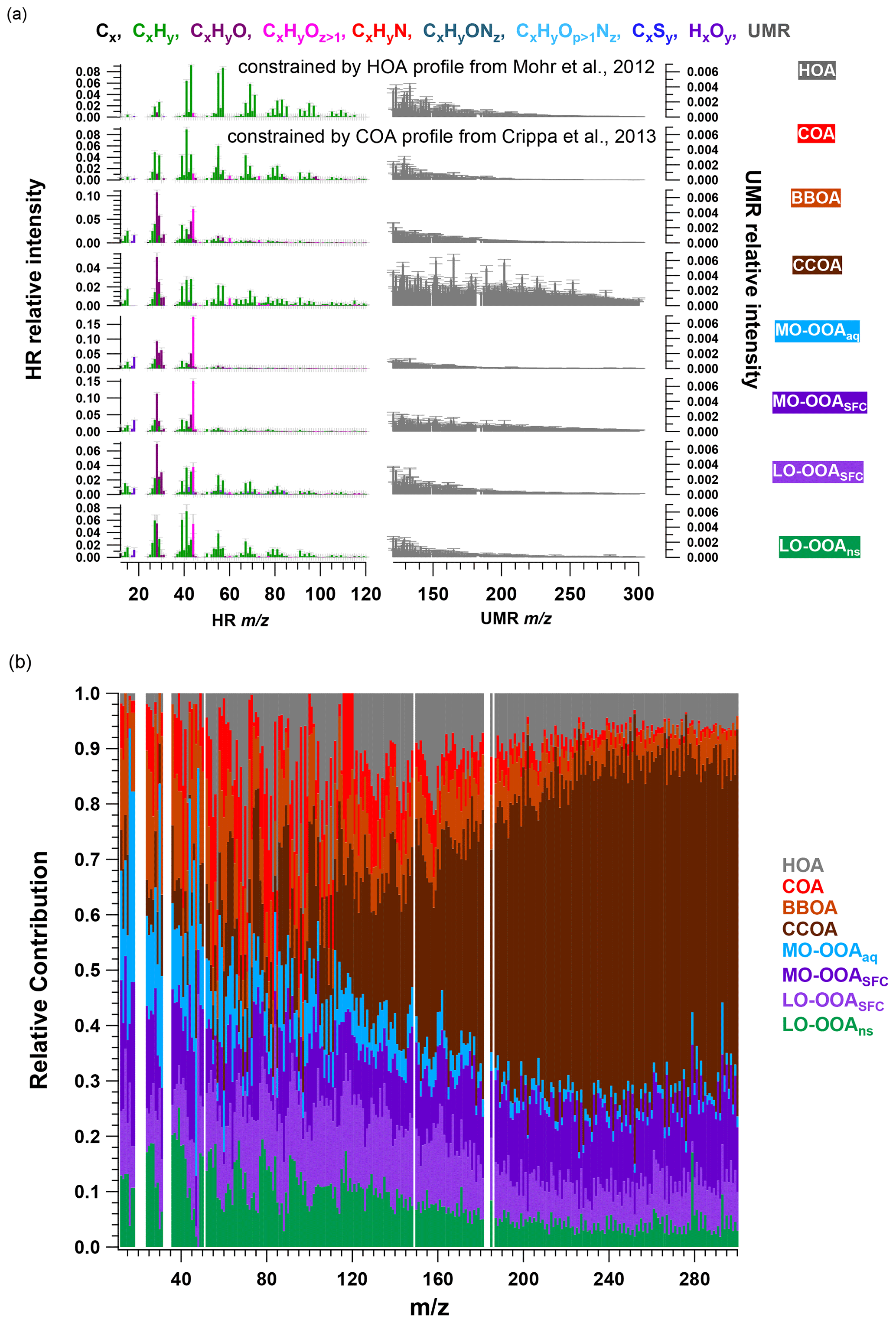
Figure 2Averaged mass spectra (a) and relative contributions (b) of the eight-factor solution from the AMS PMF bootstrap result. The mass spectra consist of HR ions from 12 to 120 and integrated integer (denoted UMR) from 121 to 300, whose intensity is multiplied by 5. In (a), error bars denote standard deviation calculated from all accepted bootstrap solutions.
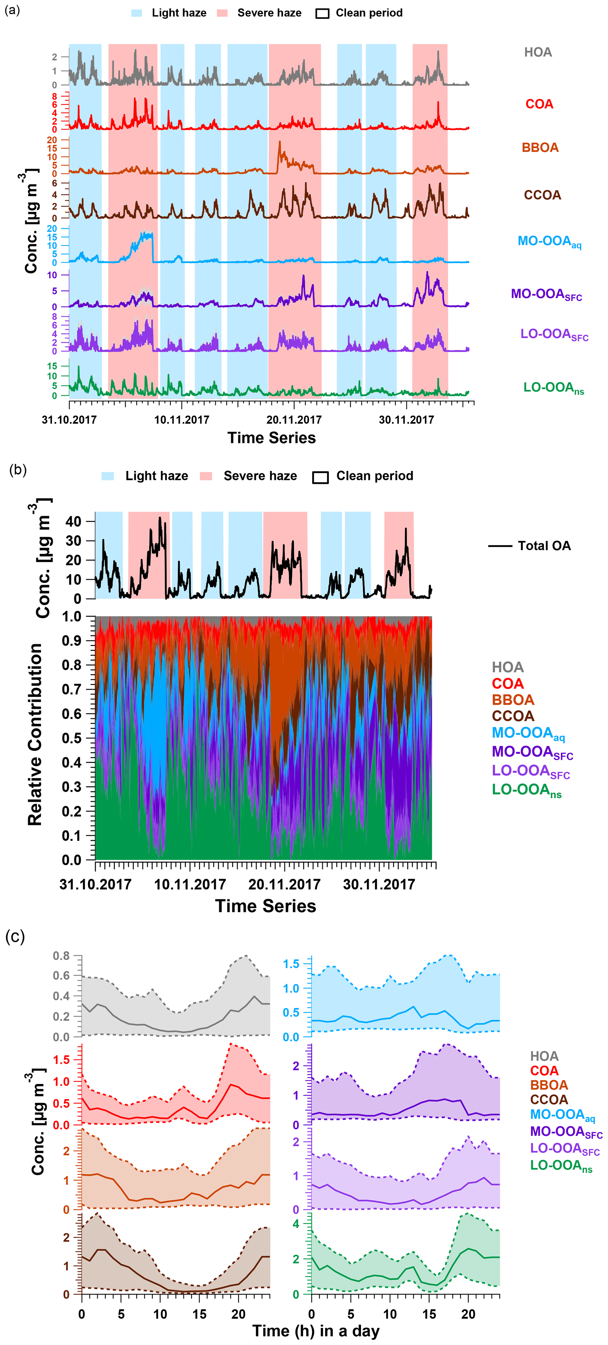
Figure 3(a) Averaged time series with interquartile range (shaded area with same colour as factor), (b) averaged total OA concentration and relative contributions and (c) median diurnal cycle the accepted AMS PMF bootstrap eight-factor solutions based on the criteria discussed in Sect. 2.3. Lower and upper dashed lines in (c) indicate first and third quantiles. In (a) and (b), the shaded areas in red and in blue represent periods of severe haze and light haze, respectively.
In selecting the PMF solution that best represents the AMS dataset, we considered both mathematical diagnostics (e.g. ) and the interpretability of the retrieved factors. Evaluation of factor interpretability includes (1) correlation of the time series with external data; (2) comparison of factor diurnal cycles with known source activity and previous measurements in Beijing; (3) identification of source-specific spectral features; and (4) differences in factor trends between heating/non-heating and/or haze/non-haze periods. Solutions from 5 to 10 factors were explored (Figs. S9 to S14), with an eight-factor solution selected as the best representation of the data according to the above criteria. Solutions with fewer than six factors showed evidence of mixed primary sources. The seven- and eight-factor solutions resolve additional OOA factors, which have clear temporal and compositional differences that support their separation and interpretation. Higher order solutions lead to uninterpretable splitting of OOA factors. Therefore, the eight-factor solution is retained for further analysis.
HOA. The HOA spectrum (Fig. 2a) is characterised by alkyl fragments, especially CnH and CnH. Major ions include C3H, C4H, and C5H (Zhao et al., 2019; Xu et al., 2019; Sun et al., 2016a; Elser et al., 2016; Zhang et al., 2014; Ng et al., 2011). It also shows good correlation with CO and eBC (r2=0.50 and 0.70, Fig. S16), which are tracers for traffic emissions (Sun et al., 2016a; Zhang et al., 2014; Chan et al., 2011). Concentrations of this factor are elevated overnight due to boundary layer dynamics and exhibit peaks from 06:00 to 09:00 and from 17:00 to 21:00, corresponding respectively to the morning and evening rush hours (Figs. 3c and S15). The averaged concentration during the evening peak (0.5 µg m−3) is almost twice as high as the morning peak (∼ 0.3 µg m−3), due to the low planetary boundary layer height and resulting accumulation of vehicle emissions at night (Sun et al., 2016a; Han et al., 2009). This diurnal pattern is consistent with other winter studies in Beijing (Sun et al., 2016a; Zhang et al., 2014). However, the averaged relative contribution of HOA factor to total mass (∼ 3.0 %) is significantly lower than previous studies (∼ 10.0 %) (Elser et al., 2016; Hu et al., 2016; Sun et al., 2016a; Zhang et al., 2014; Huang et al., 2010); this indicates that primary traffic emissions comprise a minor fraction of OA during both non-heating and heating periods.
COA. The COA spectrum contains both alkyl fragments and slightly oxygenated ions, consistent with aliphatic acids from cooking oils (Hu et al., 2016). It is typically characterised by a ratio of C3H3O+ to C3H5O+ greater than 2.0 and is 3.4 in this study (Xu et al., 2019; Zhao et al., 2019; Sun et al., 2016a, b; Crippa et al., 2013; Mohr et al., 2012). The time series of the COA factor strongly correlates with AMS C6H10O+ ( 98), a good tracer for cooking activities reported by many studies (Xu et al., 2019; Zhao et al., 2019; Elser et al., 2016; Hu et al., 2016; Sun et al., 2016a, b; Mohr et al., 2012; Sun et al., 2011), with r2=0.96 and 60.1 % of the mass of this ion being apportioned to COA. The diurnal cycle shows three peaks: from 07:00 to 09:00 LT (UTC+8) at breakfast and from 12:00 to 13:00 at lunchtime and a larger peak from 18:00 to 21:00 during dinner (Figs. 3c and S15). This three-peak diurnal pattern agrees with the diurnal cycle observed by Sun et al. (2016a) but differs from many other studies at different sites during winter in Beijing, where only two peaks are evident and the morning peak from 07:00 to 09:00 is missing. This suggests a dependence on the proximity to local emissions (Xu et al., 2019; Elser et al., 2016; Hu et al., 2016; Zhang et al., 2014). The ratio of dinner peak to lunch peak is about 2.0, similar to the values of ∼ 2.0 and 2.3 observed by Elser et al. (2016) and Hu et al. (2016), respectively, whereas Sun et al. (2016a) reported a ratio of 1.29. Overall, the COA factor is a non-negligible contributor to total OA, with a relative contribution of 6 %, lower than 18 % in 2013 (Sun et al., 2016a), 25 % in 2014, and 16 % in 2016 wintertime (Xu et al., 2019). The mean concentration is 0.3 µg m−3, lower than previous studies (Xu et al., 2019; Zhao et al., 2019; Elser et al., 2016; Hu et al., 2016; Sun et al., 2016a, b; Mohr et al., 2012; Sun et al., 2011).
BBOA. Consistent with other studies in Beijing (Zhao et al., 2019; Elser et al., 2016; Hu et al., 2016; Sun et al., 2016a), a BBOA factor was resolved. Typically, the BBOA factor mass spectrum is characterised by increased contributions from C2H4O at 60 and C3H5O at 73, which is typical of anhydrosugars such as levoglucosan (Alfarra et al., 2007; Lanz et al., 2007; Sun et al., 2011). However, although the contribution of the BBOA factor to C2H4O is the highest (28.6 %) among those factors, and its correlation is also high, with r2=0.62, other primary sources like CCOA and COA also contribute significant fractions of C2H4O signal. BBOA also correlates strongly with C3H5O (r2=0.71) and C6H6O (r2=0.81), which are also typical of biomass burning activities (Lanz et al., 2007; Sun et al., 2011). The O : C ratio and N : C ratio for this factor are 0.4 and 0.02, respectively, agreeing quite well with the values found in other studies (Xu et al., 2019; Zhao et al., 2019; Hu et al., 2016).
The BBOA time series is event-driven, with both concentrations and relative contributions increasing during haze events, especially the haze event from 18 to 22 November (68.7 % of total OA). Apart from this event, the BBOA concentration increase during other haze events is also clear, regardless of non-heating vs. heating season. Overall, the average BBOA concentration for the haze events was 1.9 µg m−3, with a maximum of 19.1 µg m−3 for the event from 18 to 22 November and ∼ 0.1 µg m−3 for the clean periods. These are both lower than the study in midwinter from 2013 to 2014 (Sun et al., 2016a) and studies from early winter in 2014 and 2016 (Xu et al., 2019). The relative contribution of BBOA to total OA is 15.4 % for haze periods and 8.2 % for the clean period, respectively, consistent with observations of Elser et al. (2016), who report 13.9 % and 8.9 % for haze and clean periods in wintertime in Beijing, respectively.
CCOA. Apart from alkyl fragments CnH and CnH, the main feature of the CCOA profile is the high contribution from PAHs (approximately 175 to 300), especially in the high range, consistent with studies from Elser et al. (2016), Zhang et al. (2008), and Xu et al. (2006). In the high mass range, PAHs contribute an increasingly higher fraction with increasing (Fig. 2b). A series of strong signals are found in the factor profile at 115 (C9H), 128, 139, 152, 165, 178, 189, 202, 215, 226, 239, and 252, which have been shown to be characteristic of aromatics and PAHs (Dzepina et al., 2007). Moreover, the time series of this factor and these ions correlate quite well with r2 of 0.81 (C9H), 0.80 ( 128), 0.83 ( 139), 0.90 ( 152), 0.90 ( 165), 0.93 ( 178), 0.94 ( 189), 0.97 ( 202), 0.97 ( 215), 0.98 ( 226), 0.96 ( 239), and 0.98 ( 252), respectively, consistent with observations from Dzepina et al. (2007), Hu et al. (2013, 2016), and Sun et al. (2016a).
Coal is widely used for domestic heating in northern China, including the greater Beijing area and surrounding provinces (Zhang et al., 2008), but is not permitted for residential use in the downtown area. Instead, beginning on 15 November, power plants using natural gas provide heating to every household in the Beijing downtown area, and municipal coal combustion starts providing heat to the surrounding area. Interestingly, the time series of the CCOA factor reflects this seasonal transition, as the mean daily maximum concentration increased from 2.9 µg m−3 before 15 November to 5.9 µg m−3 after. Similar to other studies (Elser et al., 2016; Hu et al., 2016; Sun et al., 2016a; Zhang et al., 2014), the diurnal concentration peaks at night between 21:00 and 06:00, with an average contribution of 15.5 % to total OA and decreases during the day from 07:00 to 20:00 with an average contribution of 7.4 %, consistent with domestic heating (Figs. 3c and S15). Overall, the mean contribution to total OA is 11.4 %, with 7.1 % in the non-heating period and 14.7 % in the heating season. The latter number agrees with observations conducted in the heating period in Beijing during winter, ranging from 10 % to 30 % (Elser et al., 2016; Hu et al., 2016; Zhang et al., 2014; Sun et al., 2013).
OOAs. As noted above, the OOA factors resolved here differ from previous AMS studies in Beijing, where only one or two OOA factors were resolved and classified based on volatility (semi-volatile OOA and low-volatility OOA) (Zhao et al., 2019; Zhang et al., 2014; Hu et al., 2013) or oxidation state (more-oxygenated OOA and less-oxygenated OOA) (Xu et al., 2019; Elser et al., 2016; Sun et al., 2016a, 2013). In this study, two more-oxygenated OOAs (MO-OOA) and two less-oxygenated OOA (LO-OOA) factors were resolved. The OOA factors are characterised by higher signal from CO than found in the POA factors. In this study, CO comprises approximately 15.0 % of the two MO-OOA factors. For the two LO-OOAs, the CO contribution to the total signal is only 3.8 % in LO-OOASFC and 5.4 % in LO-OOAns, while the ratio of CO to C2H3O+ is still higher than for the POAs. Moreover, a higher contribution of the CxHy group is observed in the LO-OOA factors than in the MO-OOA factors. Each OOA factor has a significantly different time series, corresponding to specific haze events and/or seasonal changes, providing a first suggestion that their separation may be meaningful.
Among the MO-OOA factors, one factor (influenced by aqueous-phase chemistry, defined as MO-OOAaq) has high absolute and relative concentrations during a single haze event from 4 to 7 November (maximum 16.2 µg m−3, > 60.0 % of the total OA mass) but is a minor component throughout the rest of the campaign. In contrast, the other MO-OOA factor (aged solid fuel combustion emissions, defined as MO-OOASFC) is a minor component before 15 November, but both its mass and relative contribution steadily increase during the heating season, especially during haze periods. This is consistent with the temporal pattern of CCOA, suggesting this factor may be linked to coal combustion activities. The temporal evolution of the two LO-OOA factors is also distinguishable. The concentration of one factor (LO-OOASFC) increases in every haze episode under stagnant conditions and is correlated with the total OA time series (r2=0.91), whereas the other factor (LO-OOAns) exhibits a clear diurnal pattern in the non-heating season, but this diurnal cycle is absent during the heating season. Interestingly, the contribution of the LO-OOAns factor to total OA is higher during the clean days, suggesting this factor may be more influenced by regional processes. The chemical characteristics and sources and processes governing these OOA factors are discussed in detail in the next section, in conjunction with the EESI-TOF analysis.
3.3 Investigation of factor composition by EESI-TOF
As discussed in Sect. 2.3, PMF of the EESI-TOF mass spectral time series was conducted on a seven-factor solution, whereby all factor time series were constrained by the seven non-HOA factors retrieved from AMS PMF. The EESI-TOF factor time series are compared to their AMS counterparts in Fig. S17, and scatter plots of EESI-TOF vs. AMS on a factor-by-factor basis are shown in Fig. S18. These comparisons suggest that the EESI-TOF factor time series mostly reflect the main trends in the AMS factor time series. This approach enables a more chemically specific interpretation of the retrieved AMS factors, which both supports POA factor identification and provides additional insight into the sources and processes governing SOA. Note that all factors resolved in this study are based on time series derived from AMS PMF analysis; therefore, in the following sections, these factors are discussed from the chemical perspective of the EESI-TOF, and no distinction is made between factors represented by PMF analysis of AMS or EESI-TOF. The PMF result of the EESI-TOF time series was used as the base case for bootstrap runs, and all the bootstrap runs were retained for further analysis. EESI-TOF factor profiles (corresponding to AMS-derived factor time series) are interpreted by (1) comparison between these factor profiles and mass spectra retrieved from a chamber study using an EESI-TOF (Amelie Bertrand, personal communication, 2019) and/or field studies (Qi et al., 2019; Stefenelli et al., 2019); and (2) identification of key ions in the factor profiles by z-score analysis introduced in Sect. 2.3.3. The time series and factor profiles of the seven-factor solution are shown in Fig. 4.
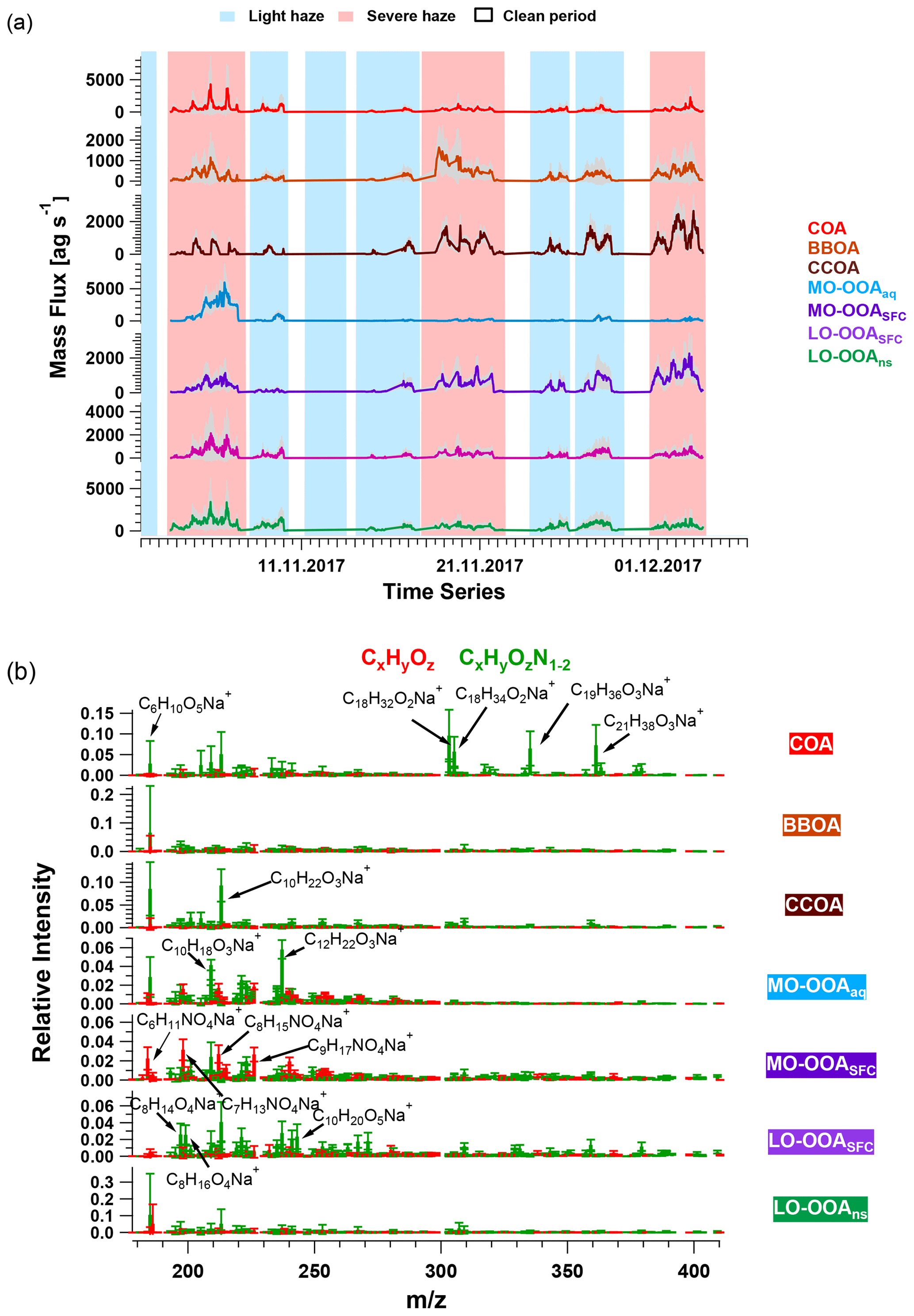
Figure 4The averaged (a) time series and (b) mass spectra of accepted solutions from combined bootstrap/a-value analysis of the EESI-TOF dataset. EESI-TOF time series are constrained by the seven non-HOA factors retrieved from AMS PMF analysis. The shaded area in (a) indicates the anchor of bootstrap/a-value analysis as shown in Eq. (6). Error bars in (b) indicate the standard deviation of each ion calculated from all selected solutions. In (a), the shaded areas in red and in blue represent severe and light haze periods, respectively.
We discuss the three primary factors in Sect. 3.3.1 and the four OOA factors individually in the subsequent sections. Carbon number distribution plots generated from the EESI-TOF factor profiles and colour-coded by different families are presented in Figs. 5 and 6 for the three POA factors and Figs. 7 and 8 for the four OOA factors. In the carbon number distribution plots, ions are classified first based on carbon numbers (x axis) and ions with the same number of carbons are further divided into different categories based on H : C and O : C ratios (colour code). Figure 9 shows Van Krevelen plots (atomic H : C vs. O : C ratio) for the four OOA factors based on AMS factor profiles coloured by the number of nitrogen atoms in each fragment and sized by the median z score across all bootstrap runs, with large markers denoting ions with a z score > 1.5.
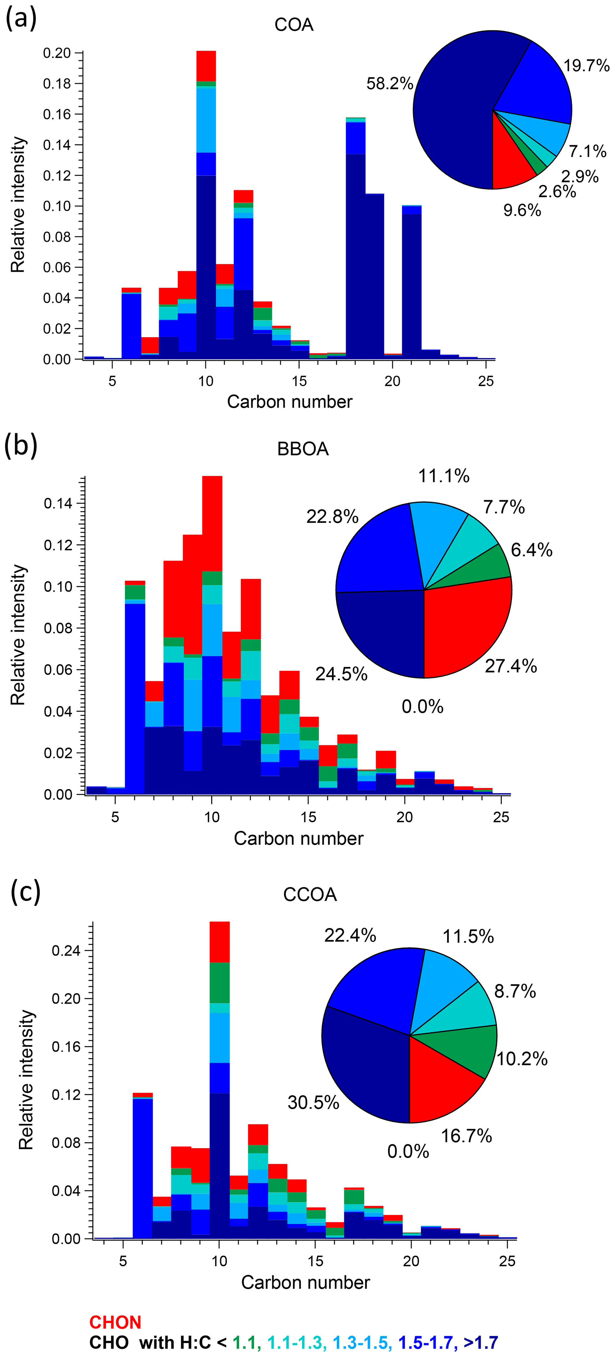
Figure 5Carbon number distribution plots of three primary factors: (a) COA, (b) BBOA, and (c) CCOA, coloured by CxHyOzN1–2, and five different CxHyOz categories based on H : C ratio (H : C < 1.1, 1.1 < H : C < 1.3, 1.3 < H : C < 1.5, 1.5 < H : C < 1.7 and H : C > 1.7). Each distribution is normalised such that its sum is 1.
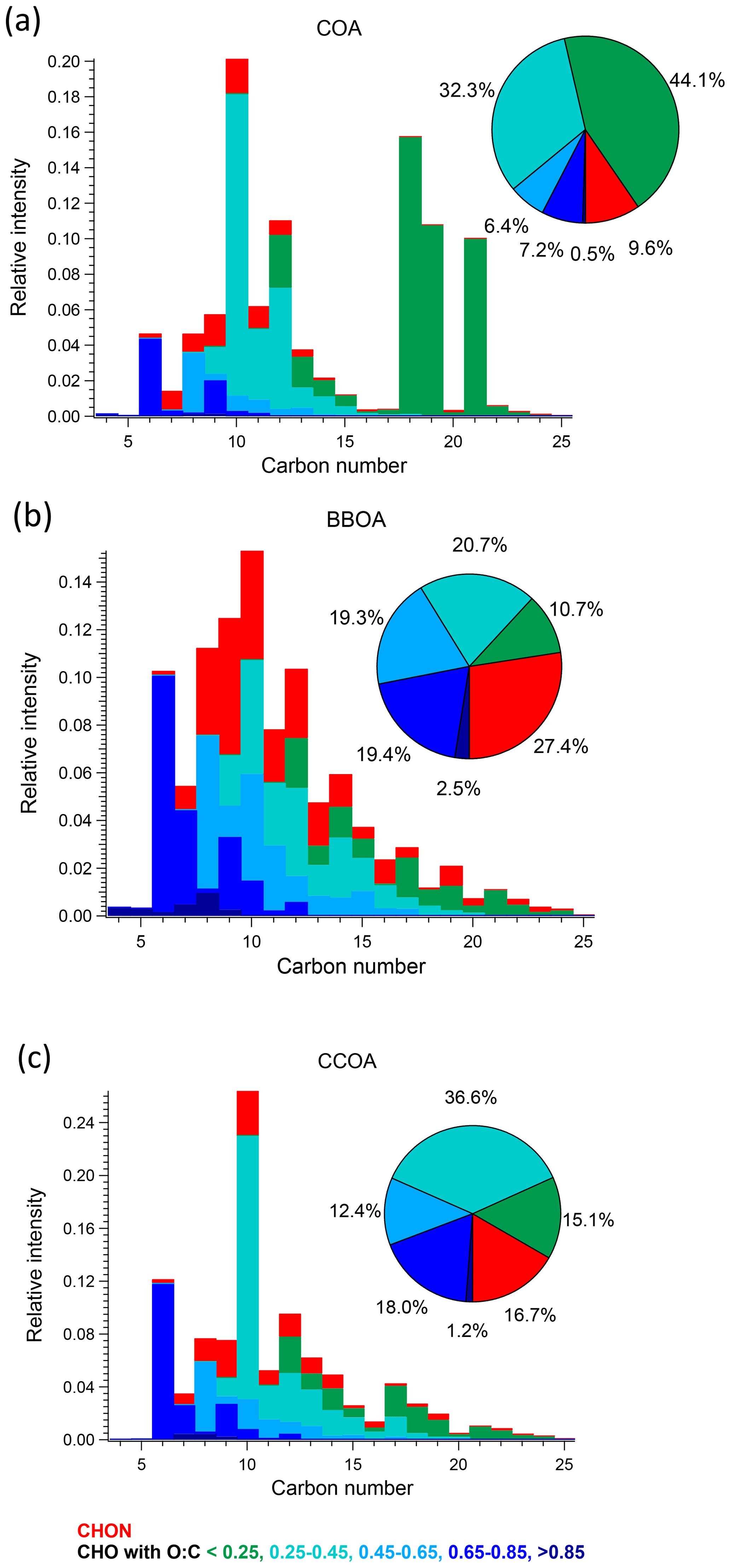
Figure 6Carbon number distribution plots of three primary factors: (a) COA, (b) BBOA, and (c) CCOA, coloured by CxHyOzN1–2, and five different CxHyOz categories based on O : C ratio (O : C < 0.25, 0.25 < O : C < 0.45, 0.45 < O : C < 0.65, 0.65 < O : C < 0.85 and O : C > 0.85). Each distribution is normalised such that its sum is 1.
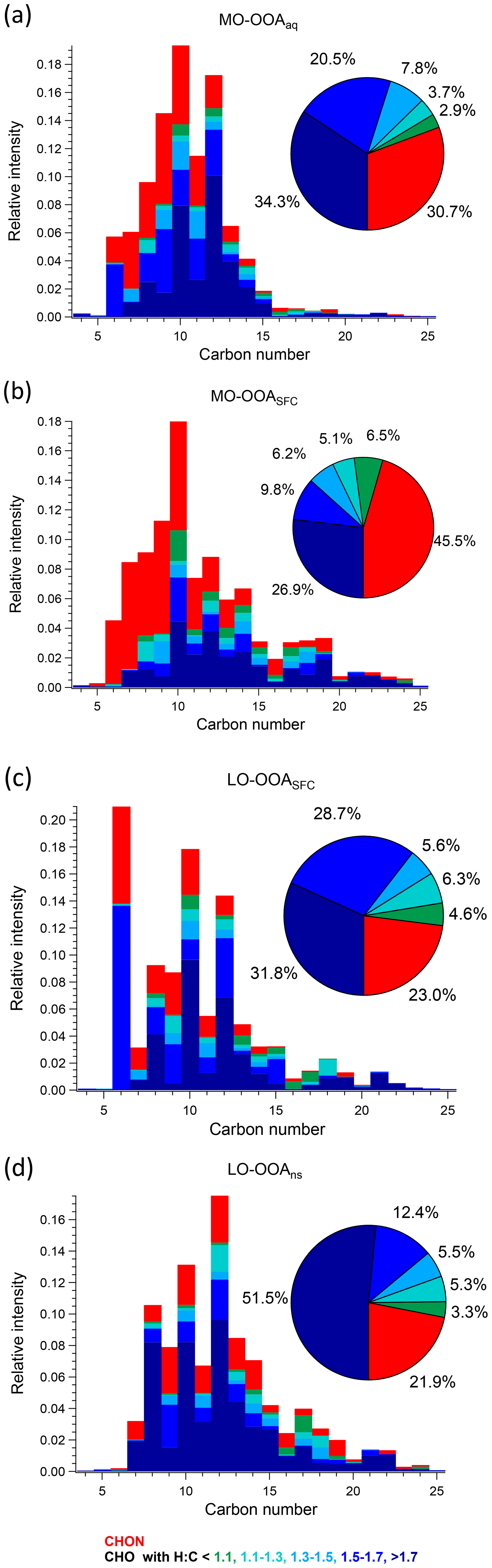
Figure 7Carbon number distribution plots of four OOA factors: (a) MO-OOAaq, (b) MO-OOASFC, (c) LO-OOASFC, and (d) LO-OOAns, coloured by CxHyOzN1–2 (red), and five different CxHyOz categories (green to blue) based on H : C ratio (H : C < 1.1, 1.1 < H : C < 1.3, 1.3 < H : C < 1.5, 1.5 < H : C < 1.7 and H : C > 1.7). Each distribution is normalised such that its sum is 1.
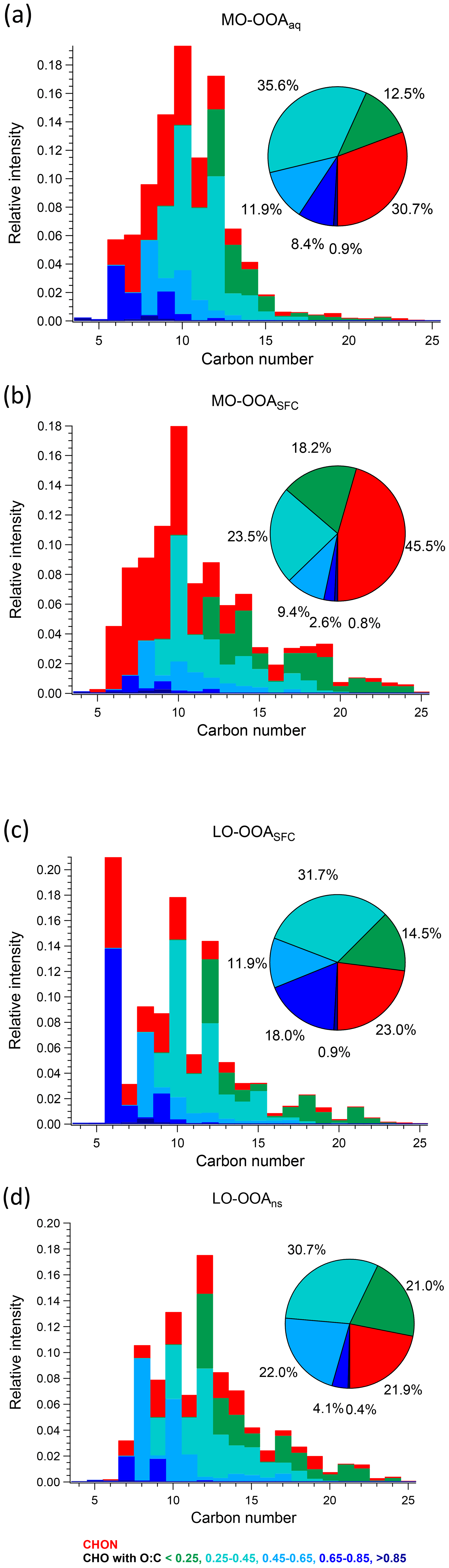
Figure 8Carbon number distribution plots of four OOA factors: (a) MO-OOAaq, (b) MO-OOASFC, (c) LO-OOASFC, and (d) LO-OOAns, coloured by CxHyOzN1–2 (red), and five different CxHyOz categories (green to blue) based on O : C ratio (O : C < 0.25, 0.25 < O : C < 0.45, 0.45 < O : C < 0.65, 0.65 < O : C < 0.85 and O : C > 0.85). Each distribution is normalised such that its sum is 1.
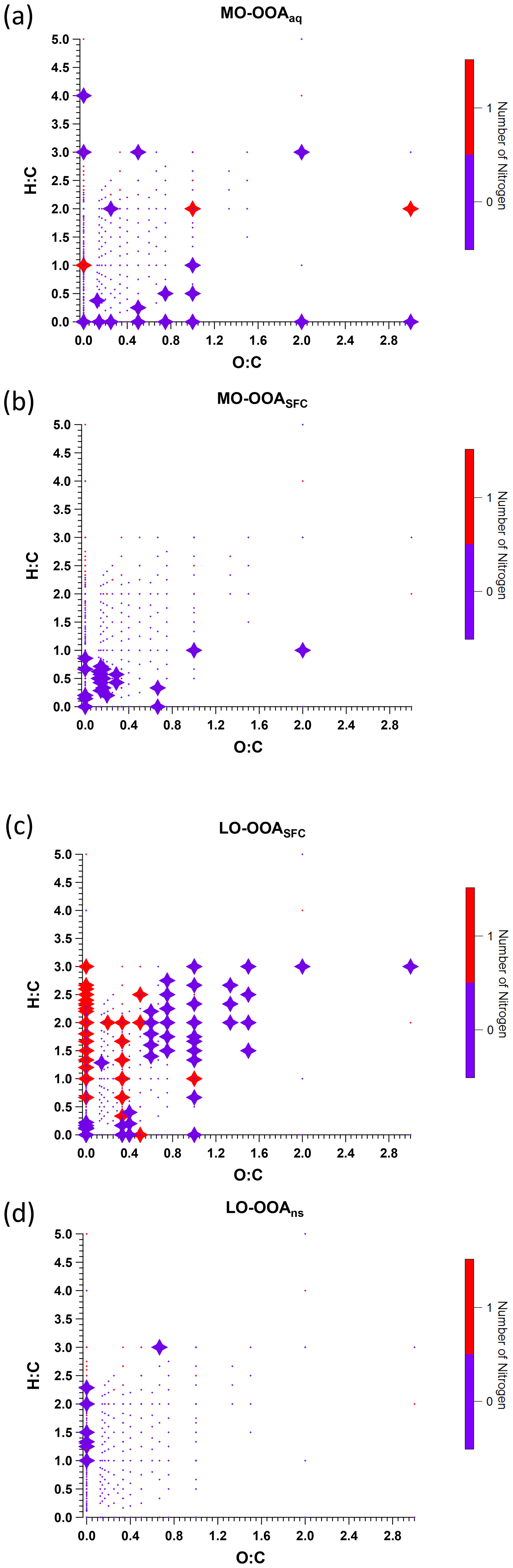
Figure 9Van Krevelen plot of AMS factor mass spectra for (a) MO-OOAaq, (b) MO-OOASFC, (c) LO-OOASFC, and (d) LO-OOAns, coloured by the number of nitrogen atoms. Large symbols denote ions with median z score ≥ 1.5, and small symbols denote median z score < 1.5 for accepted runs from bootstrap analysis.
3.3.1 POA factors
COA. Consistent with Qi et al. (2019) and Stefenelli et al. (2019), the mass spectrum of this factor (Fig. 4b) is characterised by having most of the mass at ions with high . These ions at high are likely long-chain fatty acids or/and alcohols related to cooking emission and oils (Liu et al., 2017b). For example, this factor is characterised by long-chain acids like C18H34O, C19H36O, and C21H38O, which apportion 87.2 %, 76.2 %, and 92.3 % of their total mass to this factor, and they are also unique ions in this factor, with z scores of 2.61, 2.95, and 3.34, respectively.
BBOA. The mass spectrum of BBOA (Fig. 4b) is characterised by a strong signal at C6H10O5, corresponding to levoglucosan and its isomers. Levoglucosan is a well-established tracer for primary aerosols formed from pyrolysis of cellulose in biomass burning activities. This ion contributes 6.6 % to the mass in this factor, about 4.5 times higher than the second strongest ion, consistent with previous field and laboratory measurements of biomass burning by the EESI-TOF. Both winter measurements in Zurich, Switzerland (Qi et al., 2019), and a chamber study of wood burning emissions (Amelie Bertrand, personal communication, 2019) showed levoglucosan and its isomers to be the dominant ion in EESI-TOF spectra of primary wood burning, with contributions of 13.0 % and 21.0 % respectively. In addition, the ion series C10H14Ox (x≥4) is observed in the BBOA and aged-SFC factors, consistent with Qi et al. (2019).
CCOA. As shown in the carbon number distribution plots (Figs. 5 and 6), lower H : C and O : C ratios are observed compared to other factors, especially for species with more than 10 carbons, suggesting increased contributions from aromatic acids. This is consistent with Zhang et al. (2008) who found that particles generated from industrial boilers typically contain a considerable fraction from both aromatic acids and aliphatic acids. Note that PAHs, which comprise the unique AMS spectral marker, are not detectable by the EESI-TOF extraction/ionisation scheme used here.
3.3.2 MO-OOASFC
As noted in Sect. 3.2, the AMS MO-OOASFC mass spectrum is consistent with OOA factors characteristic of SOA and represents aged, oxygenated emissions from solid fuel combustion. The carbon number distribution of the EESI-TOF MO-OOASFC mass spectrum (Fig. 7b) shows several notable features that provide further insight into its source. First, the contribution of CxHyOz ions with low H : C is significantly higher than for the other OOA factors. Specifically, (CxHyOz) comprises 11.6 % of the total signal and 20.9 % of CxHyOz; for the other non-SFC related OOA factors, (CxHyOz) comprises a maximum of 8.6 % of the total signal and 10.9 % of CxHyOz. The high fraction of low H : C ratio ions suggests a higher contribution from aromatic precursors relative to the other OOA factors. The (CxHyOz) signal is consistent with that of aged wood burning factors retrieved during winter in Zurich (13 %–14 %, Qi et al., 2019) (Fig. S19). Aged wood burning factors were also retrieved from source apportionment of wintertime EESI-TOF measurements in Magadino, located in a Swiss alpine valley (Giulia Stefenelli, personal communication, 2019), where (CxHyOz) comprises 9.0 %–23.0 % of the total signal. Different from the aged biomass burning factors found in Zurich and Magadino, C6H10O5 is not observed in MO-OOASFC, but other ions found in the aged biomass burning factors from Qi et al. (2019) and Giulia Stefenelli (personal communication, 2019), including C10H16Ox (x≥3), are also apportioned to SFC-related factors in the present study. Still, the CxHyOz distribution in the MO-OOASFC factor retrieved in Beijing differs from the previous studies in Switzerland in terms of the overall carbon number distribution. Specifically, the Swiss measurement in Magadino, a site strongly influenced by biomass burning activities (Giulia Stefenelli, personal communication, 2019), showed a peak at C6 and a peak from C8 to C10, and the chamber study on coal combustion oxidation (Amelie Bertrand, personal communication, 2019) exhibits a peak from C6 to C12, whereas in Beijing the signal is spread over a much larger range (approximately C7 to C19).
Also evident from Fig. 7 is the high contribution from CxHyOzN1–2 ions, which comprise 45.5 % of the total signal. This is significantly higher than the 18 %–25 % observed in the Zurich factors by Qi et al. (2019) but comparable to 35 %–41 % observed in Magadino. As above, the carbon number distribution of CxHyOzN1–2 differs between Beijing and Switzerland, although the trends are reversed. In Beijing, the CxHyOzN1–2 signal occurs mostly in the C6 to C10 range, with a contribution of 73.0 % to the total CxHyOzN1–2 signal, whereas for the Swiss measurements, it spans C6 to C10, with a contribution of 56 % at most to the total CxHyOzN1–2 signal, and almost evenly distributes into other bins. High-intensity CxHyOzN1–2 ions in Beijing MO-OOASFC include C6H11NO4, C7H13NO4, C8H15NO4, C9H17NO4, and C10H19NO4. The high nitrogen content in MO-OOASFC likely reflects high-NOx concentrations in the Beijing region during wintertime. In addition, ions tentatively attributed to nitrocatechol (C6H5NO4), and its homologous series (C7H7NO4, C8H9NO4) are apportioned predominantly to this factor and CCOA (see Fig. S25b and c), indicating the influence of oxidised aromatics from coal combustion emissions (Mohr et al., 2013).
Interestingly, the AMS MO-OOASFC profile and Van Krevelen plot (Fig. 9) show that the ions for which MO-OOASFC has a high z score (>1.5) predominantly exhibit low H : C ratios. These ions include C7H2O+, C7H3O+, C7H4O+, C7H5O+, C8H4O+, and C8H5O+. Although these ions are not addressed in OOA factor separation in most AMS PMF studies due to their low intensities, their high z score in the present work suggests they may contain some source-specific information. The temporal evolution of these ions is consistent with EESI-TOF ions having a low H : C ratio and thus tentatively attributed to aromatics, e.g. C12H10O8 and C16H14O6 (see Fig. S25d and e). This also suggests an elevated contribution from aromatic oxidation relative to the non-SFC-derived SOA factors. An increased contribution from EESI-TOF ions with low H : C was also observed in oxidised wood burning emissions by Qi et al. (2019).
3.3.3 LO-OOASFC
The LO-OOASFC factor mass spectrum is also consistent with solid fuel combustion but is less oxygenated than MO-OOASFC. The carbon number distribution of the EESI-TOF LO-OOASFC mass spectrum (Fig. 7c) shows a contribution of CxHyOz ions with low H : C comparable to that of MO-OOASFC. Specifically, (CxHyOz) comprises 10.9 % of the total LO-OOASFC signal, compared to 11.6 % from MO-OOASFC. This is consistent with less-aged biomass burning (LABB) factors retrieved from source apportionment of wintertime EESI-TOF data in Zurich and Magadino, where (CxHyOz) contributed 10 %–16 %. LO-OOASFC contains a substantial contribution (10.5 %) from C6H10O5 (levoglucosan and its isomers), which is substantially higher than that of MO-OOASFC (0 %) and LO-OOAns (0 %) and also than for primary BBOA (6.6 %) and CCOA (8.6 %). Interestingly, this factor has a very high fraction (31.8 %) from (CxHyOz), substantially higher than the 12 % to 14 % observed in Zurich and Magadino. It also has 18.9 % contribution from (CxHyOz), half of the fraction (∼ 40 %) of the LABB factors in Zurich and Magadino. The high H : C (1.66) and low O : C (0.41) from EESI-TOF result in low averaged carbon oxidation states (−0.87) of this factor, suggesting that this factor is less oxygenated than the LABB factors in those two studies, which had a minimum of −0.60.
Regarding nitrogen-containing species, CxHyOzN1–2 ions contribute 23.0 % to the total signal in this factor, similar to their contributions in the Zurich and Magadino LABB (17 % to 22 %). However, in Beijing a large fraction (10.7 %) of the CxHyOzN1–2 derives from a single ion (C6H11NO4). Otherwise, the carbon number distribution of CxHyOzN1–2 ions in Beijing is weighted from C7 to C10, consistent with SOA from wood burning experiments with OH or NO3 (Amelie Bertrand, personal communication, 2019) as shown in Fig. S28. Similar to the primary BBOA and CCOA factors, LO-OOASFC is elevated overnight, suggesting a contribution from nighttime chemistry and/or rapid oxidation of primary emissions.
3.3.4 MO-OOAaq
The MO-OOAaq factor time series is dominated by high absolute and relative concentrations during a haze event in the non-heating season. Both the atmospheric conditions during this event and the overall factor composition are consistent with a strong influence from SOA formed by aqueous-phase chemistry.
Figure 10a shows the time series of the CO and CO+ ions from AMS, and the corresponding scatter plot is shown in Fig. 10b. For most of the data, the ratio of CO+ to CO is approximately 1, consistent with the mean value for bulk atmospheric OA (Canagaratna et al., 2015; Aiken et al., 2008) and the assumption in the standard AMS fragmentation table. In contrast, the slope is only 0.5 for the haze event on 4 to 7 November. This relative enhancement of CO is characteristic of small acids or diacids, e.g. oxalic acid, malonic acid, and succinic acid (Canagaratna et al., 2015), shown in Fig. S22. These molecules can enter the particle via solvation, potentially followed by aqueous-phase chemistry (Tan et al., 2012, 2010; Carlton et al., 2007; Ervens et al., 2004), or as condensation products of gas-phase reactions (Mehra et al., 2020; Wang et al., 2020; Zaytsev et al., 2019; Legrand et al., 2005; Sellegri et al., 2003; Sempere and Kawamura, 1994). For example, Lamkaddam et al. (2021) have shown that up to 70 % of isoprene oxidation products can be dissolved in a water film. However, because aqueous reaction pathways under subsaturated conditions favour the uptake of highly soluble molecules such as small acids/diacids, their contribution relative to larger oxygenates is increased, consistent with the lower slope observed here.
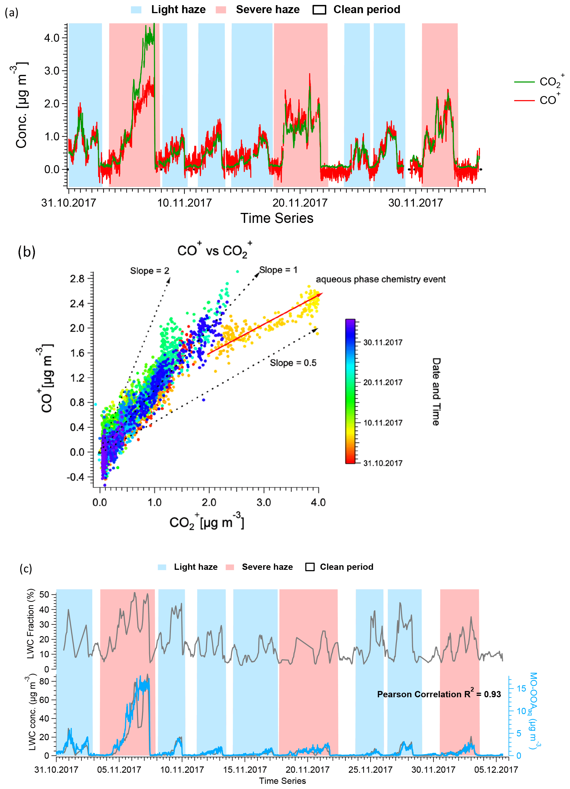
Figure 10(a) Time series of AMS-measured CO+ and CO throughout the campaign. (b) Scatter plot of CO+ and CO, indicating a different slope for the haze event between 4 and 7 November 2017, suggesting aqueous-phase chemistry may happen in this period. (c) Time series of LWC, both in fraction (top) and mass concentration (bottom), complemented by MO-OOAaq, demonstrating the high correlation between the latter two variables. In (a) and (c), the shaded areas in red and in blue represent severe and light haze periods, respectively.
An enhanced contribution from small acids is also suggested by the EESI-TOF MO-OOAaq profile. As shown in Figs. 7 and 8, MO-OOAaq has enhanced signal from ions with low carbon number relative to the other OOA factors. Further, Fig. 7 shows that these low-C ions are highly oxygenated (e.g. C6H6O5), which is likewise consistent with small multifunctional acids and polyacids. The EESI-TOF spectra thus provide further support for the attribution of this factor to the processes discussed in the previous paragraph. However, the carbon number distribution in Fig. 7a shows (CxHyOz) comprises only 6.6 % of the total signal, suggesting these acids are unlikely formed by oxidation of aromatic precursors. Note that due to the application of the volatility-based filter for distinguishing particle phase vs. spurious ions (see Sect. S3), the contribution of such small, highly oxygenated ions presented here represents a lower limit.
As shown in Figs. 3 and 11, MO-OOAaq provides a major fraction of 40.8 % to the total OA during the major haze event on 4 to 7 November (peak concentration >40 µg m−3). In fact, OA concentrations during this event are at least as high as those observed during the heating period, despite the likelihood of reduced concentrations of precursor VOCs due to the mandated reductions in combustion activities related to domestic heating in rural areas. We therefore investigate the reasons for the high SOA production during this specific event. The aerosol liquid water content (LWC) was calculated from ISORROPIA-II (Fountoukis and Nenes, 2007), and a high LWC is typically associated with aqueous-phase chemistry. The LWC concentration is presented in Fig. 10, together with the time series of MO-OOAaq. The two time series are strongly correlated (r2=0.93), and both are dramatically higher during the 4 to 7 November event than for the rest of the study, suggesting the role of the aqueous-phase chemistry in this haze event. Note that the strong correlation between MO-OOAaq and LWC is not driven solely by the event on 4 to 7 November; rather, the two time series are remarkably well correlated throughout the entire campaign. This further supports the interpretation of MO-OOAaq as being characteristic of aqueous SOA production throughout the campaign, rather than being characteristic of only a single event.

Figure 11Time series of total OA and the mean contribution of eight AMS factors in each haze event and clean periods for the non-heating and heating periods. The top two pie charts indicate the averaged contributions for clean periods in non-heating season and heating season, and the three middle and six bottom pie charts indicate the corresponding averaged contributions for three severe haze events (red shaded area) and six light haze events (blue shaded area) according to the time series of total OA below.
The question arises as to whether MO-OOAaq reflects the irreversible production of SOA via aqueous pathways or instead reversible solvation of volatile and semi-volatile organics. To assess this, we look in detail at the MO-OOAaq and LWC correlations during the 4 to 7 November event (shown in Fig. 10) and change of MO-OOAaq in every 2 h interval (Fig. S24). The most significant disagreement between the time series occurs from 08:00 to 23:00 on 6 November, when the LWC sharply decreases while MO-OOAaq remains high. If MO-OOAaq were driven by reversible solvation, this extended decrease in LWC would be expected to drive a corresponding decrease in MO-OOAaq. However, the MO-OOAaq concentrations appear unaffected by the decrease in LWC, suggesting that the MO-OOAaq does indeed consist of irreversibly generated SOA via aqueous chemistry.
The reasons for the high LWC are driven by the combination of high RH and high inorganic fraction (especially NH4NO3), which as shown in Fig. 1 are both maximised during this period. The high NH4NO3 content during 4 to 7 November is in turn driven by a unique air mass source region. Figure 12a shows 72 h backward trajectories calculated from the HYSPLIT transport model (Rolph et al., 2017; Stein et al., 2015) and analysed in Zefir v 4.0 (Petit et al., 2017). Trajectories are coloured by date and time. In the figure, trajectories from 4 to 7 November pass over regions of high-NOx emissions to the east and south of Beijing (Shandong and Henan provinces) before arriving at the sampling site. The air parcel spends approximately 30 h over these high-NOx regions, as shown in Fig. 12b. As shown in Fig. S29, the period of 4 to 7 November is the only time in the campaign during which the back trajectories pass over this region. Due to the high NO2 concentration and high RH in this period, particulate nitrate is produced during this regional transport homogeneously and/or heterogeneously, resulting in water uptake and high LWC in the aerosol phase. The high LWC in turn facilitates further heterogeneous formation of nitrate. This positive feedback provides favourable conditions for efficient aqueous chemistry and thus production of MO-OOAaq (Kuang et al., 2020).
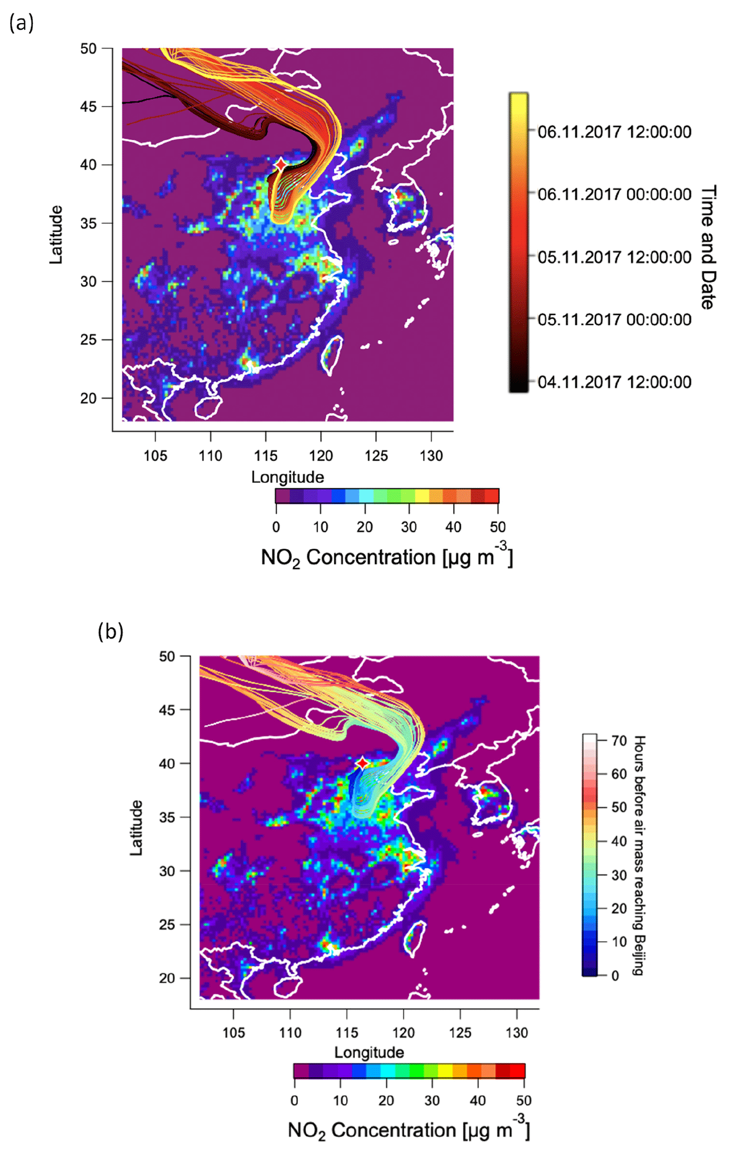
Figure 12Air mass trajectory analysis. (a) 72 h back-trajectories (HYSPLIT) for the haze event from 4 to 7 November, colour-coded by date and time, (b) 72 h back-trajectories for the haze event from 4 to 7 November, colour-coded by hours before the air mass reaches Beijing. In both figures, trajectories are overlaid on a 2015 map of surface NO2 concentrations based on the CHIMERE model and driven by the 2015 DECSO inventory (Liu et al., 2018).
3.3.5 LO-OOAns
In Sect. 3.2, this factor has been identified as LO-OOA because of its moderately high CO signal and non-negligible contribution from the CxHy group. The time series of this factor shows clear diurnal variation, which peaks at around 20:00 in the non-heating season (Fig. 3a and c), but this variation is not clear in the heating season. In addition, the contribution of this factor to total OA is higher in the clean period than during the haze events (Fig. 3b), indicating this may be related to regional sources and processes rather than more local SFC emissions. The diurnal cycle of this factor is similar to COA and LO-OOASFC, but the chemical characteristics of these three factors are different. Compared to LO-OOASFC, this factor is characterised by ions with high H : C and low O : C and does not have a significant contribution from C6H10O5, a key ion in SFC-related LO-OOAs identified in both the present and previous studies (Qi et al., 2019). LO-OOAns also does not have large contributions from ions with the aromatic feature of low H : C. Although the spectrum of COA is also characterised by ions with high H : C and low O : C, the carbon number distribution plots of COA are characterised by significant signal from long-chain acids at high carbon number, whereas the carbon number distribution of this factor is characterised by high signal at low carbon number (from C8 to C12). Compared to other OOA factors, this factor has the lowest O : C ratio (0.33) and highest H : C ratio (1.69) from EESI-TOF. Since it is not characterised by any source-specific ions or signatures identified in previous EESI-TOF studies (e.g. levoglucosan and its isomers), this factor is named as LO-OOAns, representing non-source-specific LO-OOA.
As discussed in Sect. 3.1, meteorological conditions are responsible for an alternating occurrence of haze and clean periods, and these effects from meteorology are well understood (Duan et al., 2020, 2019; Zhao et al., 2019; Xu et al., 2019; Sun et al., 2016a, b). In addition, meteorology can also influence air mass trajectories on the regional scale and mesoscale, which may further influence the aerosol chemical composition. By comparing measurements before and after the start of the heating season (15 November), the effects of heating emissions on clean and haze periods in Beijing can be assessed. Figure 11 shows the time series of total OA and the contribution of different factors to each haze event. Systematic differences between seasons suggest the influences of different sources and processes.
Clean periods in both the non-heating and heating seasons are dominated by SOA, comprising 76.9 % in the non-heating season and 70.3 % in the heating season. In both seasons, the single largest component is LO-OOAns (45.3 % and 33.2 % in the non-heating and heating seasons, respectively), consistent with its identification as regional SOA not specific to a single emissions source. The SFC fraction is higher in the heating season, with CCOA and BBOA jointly comprising 22.7 % (vs. 15.0 % in the non-heating season) and LO-OOASFC and MO-OOASFC jointly comprising 25.1 % (vs. 19.2 % non-heating season).
Seasonal differences become more pronounced under haze conditions. Three light haze events (maximum concentrations between 15.4 and 30.8 µg m−3) were observed in each season. During these events in the non-heating season, LO-OOAns remains the single largest component (33.0 % to 42.7 %), although its fraction is slightly reduced relative to clean conditions (45.3 %). There is no corresponding fractional increase observed in any of the other factors, but rather a relative increase in all across the board, which results in a slightly increased POA fraction (ranging from 29.1 % to 37.5 %, vs. 23.1 % under clean conditions). These changes likely result from an increased role of local emissions and reactivity under the stagnant conditions giving rise to haze. The non-heating light haze events contrast strongly with the heating light haze, where there is a larger reduction in the LO-OOAns fraction (at least 33.0 % in non-heating season to at most 29.6 % in heating season) that corresponds specifically to increased SFC POA (at most 26.7 % in non-heating season to at least 27.5 % in heating season). Interestingly, the SFC SOA fraction is not significantly higher than under clean conditions, although event-to-event variation is large (ranging from 20.3 % to 41.0 % under heating season haze vs. 25.1 % under clean conditions).
In general, the light haze events within a given season are relatively similar to each other. However, significant differences in composition are observed between the light and severe haze events within a given season. The two severe haze events occurring within the heating season are also quite different from each other. The conclusions that can be drawn from this observation are limited by the small number of severe haze events sampled (one non-heating, two heating) but suggest the potential for unique meteorological and transport phenomena that may affect sources and composition during the most extreme events. For example, the non-heating haze event (4 to 7 November) is dominated by MO-OOAaq from aqueous processes (40.8 % of OA) and, as discussed in the previous section, corresponds to unique air mass back-trajectories over high-NOx regions. The event from 18 to 22 November is dominated by SFC, especially BBOA, which comprises 35.8 % of OA (with CCOA contributing an additional 12.5 %), while SFC SOA comprises an only slightly larger fraction (27.8 % of OA) than under clean conditions. In contrast, the severe haze event from 30 November to 3 December has a large contribution from both SFC POA (32.8 %) and SFC SOA (41.0 %). Interestingly, the temporal evolution of these two events is also different, with the 18 to 22 November event (high SFC POA) commencing with a sudden concentration increase but remaining relatively stable thereafter, while concentrations during the 30 November to 3 December event (high SFC POA and SOA) increase gradually over multiple days. However, a close inspection of the 18 to 22 November event in Fig. 3b shows a decrease in the BBOA fraction and increase in MO-OOASFC as the event proceeds, suggesting a generally important role for local SOA formation in a stagnant air mass during the course of a haze event.
As a conclusion, our observation suggests that the sources and processes giving rise to haze events in Beijing are variable and seasonally dependent. Two salient features are observed: (1) in the heating season, SOA formation is driven by oxidation of aromatics from solid fuel combustion, with secondary SFC-related factors (i.e. sum of MO-OOASFC and LO-OOASFC) contributing 37.2 % to 72.8 % of total SOA; and (2) under high-NOx and RH conditions, aqueous-phase chemistry may make a major contribution to SOA formation (with MO-OOAaq comprising 53.7 % of total SOA). The combination of high inorganic content and aqueous SOA can yield total mass concentrations comparable to those observed in the heating season, despite reduced regional VOC emissions in the absence of heating processes.
Back-trajectory analysis shows that from 4 to 7 November, the air masses passed through a high NO2 concentration region and remained for more than 24 h in this region (Fig. 12), which facilitated nitrate formation in the aerosol phase and thus water uptake. This suggests that meteorology cannot only influence the haze evolution on a local scale but can also affect aerosol chemistry and chemical composition by influencing the origin and pathway of air mass.
From a technical perspective, a surprising outcome of this source apportionment analysis was the extent to which the AMS SOA factor profiles contained source-related information corroborating the chemically more specific measurements of the EESI-TOF. Specifically, the SFC-related factors exhibited systematic enhancements in ions with low H : C ratios, while the ratio clearly higher than 1 was found to be a clear indicator for aqueous-phase chemical processing. Although the latter observation requires the improved mass resolution of the L-TOF-AMS and is therefore not retrievable from most existing AMS datasets, taken together they suggest that AMS SOA spectra may contain more source-specific information than is typically recognised. Although these results represent a single case study and so should not be overinterpreted, we suggest that intensity-independent statistical tools such as the z-score analysis employed here may be effective in retrieving such information and in providing additional insight into SOA sources. The combination of quantitative AMS data with semi-quantitative EESI-TOF measurements is also shown to be promising, and alternative methods for combining such datasets (e.g. as discussed in the Methods section) should be pursued.
OA sources were investigated in Beijing during an intensive field deployment of AMS and EESI-TOF instruments from late September to mid-December 2017, covering the transition from the non-heating to heating seasons. This represents the first deployment of the EESI-TOF in a heavily polluted city. The robust quantification of the AMS and high chemical resolution of the EESI-TOF are shown to be highly complementary, facilitating identification of the sources and processes governing SOA concentrations. An integrated source apportionment study was conducted, by the application of PMF to AMS-only data to determine factor time series, followed by PMF on EESI-TOF-only data using AMS-derived factor time series as constraints, to increase the chemical information associated with each factor. The chemical interpretation of the AMS-determined factors was facilitated using z-score analysis and carbon number distribution plots, which successfully resolved and interpreted four SOA sources and processes.
The source apportionment analysis yielded four primary factors and four secondary factors. Primary factors were hydrocarbon-like OA (HOA), characterised by a high fraction of hydrocarbon fragments; cooking-related OA (COA), characterised by long-chain fatty acids; biomass burning OA (BBOA), with a high contribution from levoglucosan; and coal combustion OA (CCOA), with a high PAH signal at a high range. The secondary factors consisted of more- and less-oxygenated oxygenated organic aerosol from solid fuel combustion (MO-OOASFC and LO-OOASFC), more-oxygenated aerosol from aqueous-phase chemistry (MO-OOAaq), and less-oxygenated OA from mixed or indeterminate sources (LO-OOAns). The SFC-related factors were characterised by a low H : C ratio in both the EESI-TOF and AMS spectra and increased concentrations during the heating period. MO-OOAaq was characterised by an increased contribution from small, highly oxygenated ions and a low AMS ratio; taken together, these observations suggest an enhanced contribution from small acids and diacids.
The OA composition in Beijing is dominated by organic aerosols, with a high SOA fraction (66.4±13.5 %) of total OA throughout the campaign. SOA formation during the heating season derives mainly from solid fuel combustion. However, even during the non-heating season when solid fuel combustion was not a major source, an intense haze event was observed, with OA concentrations comparable to the highest concentrations observed during the heating season. These high concentrations were due to substantial SOA production from aqueous-phase chemistry and corresponded to the passage of air parcels over the high-NOx regions to the east and south of Beijing. This suggests that aqueous chemistry may provide a major contribution to SOA formation under certain meteorological conditions, even during periods of intense haze.
The data presented in the text and figures are available in the Zenodo online repository (https://doi.org/10.5281/zenodo.4681762, Tong et al., 2021).
The supplement related to this article is available online at: https://doi.org/10.5194/acp-21-9859-2021-supplement.
JGS, ASHP, JC, and RJH initiated the experiment. YT was in charge of the Beijing campaign. JD, YG, and HZ provided necessary coordination during the campaign. YT, VP, LQ, JD, YG, VK, PR, GS, LW, YW, HZ, and JGS were involved in the measurement campaign. YT mainly analysed the AMS and EESI-TOF data and performed PMF analysis. VP, LQ, and GS provided support for AMS and EESI-TOF data analysis and PMF interpretation. LW, PR, HZ, RJH, and JC provided data collected from supporting measurements. All authors from PSI (YT, VP, LQ, VK, PR, GS, LW, UB, ASHP, and JGS) contributed to the data interpretation. All authors contributed to the manuscript revision.
The authors declare that they have no conflict of interest.
Publisher's note: Copernicus Publications remains neutral with regard to jurisdictional claims in published maps and institutional affiliations.
We gratefully acknowledge the contribution from Fei Liu from NASA for providing NOx emission map of China. We also acknowledge the NOAA Air Resources Laboratory (ARL) for the provision of the HYSPLIT transport and dispersion model and READY website (https://www.ready.noaa.gov, last access: 24 June 2021) used in this publication. Logistical support from André Teixeira (Paul Scherrer Institut) and Yunfei Wu (Institute of Atmospheric Physics, Chinese Academy of Sciences) and coordination support from Chunying Chen (National Center for Nanoscience and Technology, Chinese Academy of Sciences) are gratefully acknowledged.
This study was funded by the Swiss National Science Foundation starting grant BSSGI0_155846 (IPR-SHOP), the EU Horizon 2020 Framework Programme via the ERA-PLANET project SMURBS (grant agreement no. 689443), the National Research Program for Key Issues in Air Pollution Control (grant no. DQGG0105), the National Natural Science Foundation (grant nos. 21661132005 and 41925015), and the Chinese Academy of Sciences (grant no. ZDBS-LY-DQC001). We also acknowledge the contributions of the SNF projects 200020_188624, 200021_162448, and IZLCZ2_169986 and the SDC Clean Air China Programme (grant no. 7F-09802.01.03).
This paper was edited by James Allan and reviewed by two anonymous referees.
Äijälä, M., Heikkinen, L., Fröhlich, R., Canonaco, F., Prévôt, A. S. H., Junninen, H., Petäjä, T., Kulmala, M., Worsnop, D., and Ehn, M.: Resolving anthropogenic aerosol pollution types – deconvolution and exploratory classification of pollution events, Atmos. Chem. Phys., 17, 3165–3197, https://doi.org/10.5194/acp-17-3165-2017, 2017.
Aiken, A. C., Decarlo, P. F., Kroll, J. H., Worsnop, D. R., Huffman, J. A., Docherty, K. S., Ulbrich, I. M., Mohr, C., Kimmel, J. R., Sueper, D., Sun, Y., Zhang, Q., Trimborn, A., Northway, M., Ziemann, P. J., Canagaratna, M. R., Onasch, T. B., Alfarra, M. R., Prevot, A. S. H., Dommen, J., Duplissy, J., Metzger, A., Baltensperger, U., and Jimenez, J. L.: and ratios of primary, secondary, and ambient organic aerosols with high-resolution time-of-flight aerosol mass spectrometry, Environ. Sci. Technol., 42, 4478–4485, https://doi.org/10.1021/es703009q, 2008.
Alfarra, M. R., Prevot, A. S. H., Szidat, S., Sandradewi, J., Weimer, S., Lanz, V. A., Schreiber, D., Mohr, M., and Baltensperger, U.: Identification of the mass spectral signature of organic aerosols from wood burning emissions, Environ. Sci. Technol., 41, 5770–5777, https://doi.org/10.1021/es062289b, 2007.
Allan, J. D., Alfarra, M. R., Bower, K. N., Williams, P. I., Gallagher, M. W., Jimenez, J. L., McDonald, A. G., Nemitz, E., Canagaratna, M. R., Jayne, J. T., Coe, H., and Worsnop, D. R.: Quantitative sampling using an Aerodyne aerosol mass spectrometer: 2. Measurements of fine particulate chemical composition in two UK cities J. Geophys. Res.-Atmos., 108, 4091, https://doi.org/10.1029/2002JD002359, 2003a.
Allan, J. D., Jimenez, J. L., Williams, P. I., Alfarra, M. R., Bower, K. N., Jayne, J. T., Coe, H., and Worsnop, D. R.: Quantitative sampling using an Aerodyne aerosol mass spectrometer: 1. Techniques of data interpretation and error analysis (vol 108, art no 4090, 2003), J. Geophys. Res.-Atmos., 108, 4090, https://doi.org/10.1029/2002JD002358, 2003b.
An, Z., Huang, R.-J., Zhang, R., Tie, X., Li, G., Cao, J., Zhou, W., Shi, Z., Han, Y., Gu, Z., and Ji, Y.: Severe haze in northern China: A synergy of anthropogenic emissions and atmospheric processes, P. Natl. Acad. Sci. USA, 116, 8657–8666, https://doi.org/10.1073/pnas.1900125116, 2019.
Beelen, R., Raaschou-Nielsen, O., Stafoggia, M., Andersen, Z. J., Weinmayr, G., Hoffmann, B., Wolf, K., Samoli, E., Fischer, P., Nieuwenhuijsen, M., Vineis, P., Xun, W. W., Katsouyanni, K., Dimakopoulou, K., Oudin, A., Forsberg, B., Modig, L., Havulinna, A. S., Lanki, T., Turunen, A., Oftedal, B., Nystad, W., Nafstad, P., De Faire, U., Pedersen, N. L., Ostenson, C. G., Fratiglioni, L., Penell, J., Korek, M., Pershagen, G., Eriksen, K. T., Overvad, K., Ellermann, T., Eeftens, M., Peeters, P. H., Meliefste, K., Wang, M., Bueno-de-Mesquita, B., Sugiri, D., Kramer, U., Heinrich, J., de Hoogh, K., Key, T., Peters, A., Hampel, R., Concin, H., Nagel, G., Ineichen, A., Schaffner, E., Probst-Hensch, N., Kunzli, N., Schindler, C., Schikowski, T., Adam, M., Phuleria, H., Vilier, A., Clavel-Chapelon, F., Declercq, C., Grioni, S., Krogh, V., Tsai, M. Y., Ricceri, F., Sacerdote, C., Galassi, C., Migliore, E., Ranzi, A., Cesaroni, G., Badaloni, C., Forastiere, F., Tamayo, I., Amiano, P., Dorronsoro, M., Katsoulis, M., Trichopoulou, A., Brunekreef, B., and Hoek, G.: Effects of long-term exposure to air pollution on natural-cause mortality: an analysis of 22 European cohorts within the multicentre ESCAPE project, Lancet, 383, 785–795, https://doi.org/10.1016/S0140-6736(13)62158-3, 2014.
Brown, W. L., Day, D. A., Stark, H., Pagonis, D., Krechmer, J. E., Liu, X., Price, D. J., Katz, E. F., DeCarlo, P. F., Masoud, C. G., Wang, D. S., Hildebrandt Ruiz, L., Arata, C., Lunderberg, D. M., Goldstein, A. H., Farmer, D. K., Vance, M. E., and Jimenez, J. L.: Real-time organic aerosol chemical speciation in the indoor environment using extractive electrospray ionization mass spectrometry, Indoor Air, 31, 141–155, https://doi.org/10.1111/ina.12721, 2021.
Bryant, D. J., Dixon, W. J., Hopkins, J. R., Dunmore, R. E., Pereira, K. L., Shaw, M., Squires, F. A., Bannan, T. J., Mehra, A., Worrall, S. D., Bacak, A., Coe, H., Percival, C. J., Whalley, L. K., Heard, D. E., Slater, E. J., Ouyang, B., Cui, T., Surratt, J. D., Liu, D., Shi, Z., Harrison, R., Sun, Y., Xu, W., Lewis, A. C., Lee, J. D., Rickard, A. R., and Hamilton, J. F.: Strong anthropogenic control of secondary organic aerosol formation from isoprene in Beijing, Atmos. Chem. Phys., 20, 7531–7552, https://doi.org/10.5194/acp-20-7531-2020, 2020.
Canagaratna, M. R., Jayne, J. T., Jimenez, J. L., Allan, J. D., Alfarra, M. R., Zhang, Q., Onasch, T. B., Drewnick, F., Coe, H., Middlebrook, A., Delia, A., Williams, L. R., Trimborn, A. M., Northway, M. J., DeCarlo, P. F., Kolb, C. E., Davidovits, P., and Worsnop, D. R.: Chemical and microphysical characterization of ambient aerosols with the aerodyne aerosol mass spectrometer, Mass Spectrom. Rev., 26, 185–222, https://doi.org/10.1002/mas.20115, 2007.
Canagaratna, M. R., Jimenez, J. L., Kroll, J. H., Chen, Q., Kessler, S. H., Massoli, P., Hildebrandt Ruiz, L., Fortner, E., Williams, L. R., Wilson, K. R., Surratt, J. D., Donahue, N. M., Jayne, J. T., and Worsnop, D. R.: Elemental ratio measurements of organic compounds using aerosol mass spectrometry: characterization, improved calibration, and implications, Atmos. Chem. Phys., 15, 253–272, https://doi.org/10.5194/acp-15-253-2015, 2015.
Canonaco, F., Crippa, M., Slowik, J. G., Baltensperger, U., and Prévôt, A. S. H.: SoFi, an IGOR-based interface for the efficient use of the generalized multilinear engine (ME-2) for the source apportionment: ME-2 application to aerosol mass spectrometer data, Atmos. Meas. Tech., 6, 3649–3661, https://doi.org/10.5194/amt-6-3649-2013, 2013.
Carlton, A. G., Turpin, B. J., Altieri, K. E., Seitzinger, S., Reff, A., Lim, H. J., and Ervens, B.: Atmospheric oxalic acid and SOA production from glyoxal: Results of aqueous photooxidation experiments, Atmos. Environ., 41, 7588–7602, https://doi.org/10.1016/j.atmosenv.2007.05.035, 2007.
Chan, Y. C., Hawas, O., Hawker, D., Vowles, P., Cohen, D. D., Stelcer, E., Simpson, R., Golding, G., and Christensen, E.: Using multiple type composition data and wind data in PMF analysis to apportion and locate sources of air pollutants, Atmos. Environ., 45, 439–449, https://doi.org/10.1016/j.atmosenv.2010.09.060, 2011.
Chow, J. C., Bachmann, J. D., Wierman, S. S. G., Mathai, C. V., Malm, W. C., White, W. H., Mueller, P. K., Kumar, N., and Watson, J. G.: Visibility: Science and regulation – Discussion, J. Air Waste Manage., 52, 973–999, https://doi.org/10.1016/j.atmosenv.2010.09.060, 2002.
Crippa, M., El Haddad, I., Slowik, J. G., DeCarlo, P. F., Mohr, C., Heringa, M. F., Chirico, R., Marchand, N., Sciare, J., Baltensperger, U., and Prévôt, A. S. H.: Identification of marine and continental aerosol sources in Paris using high resolution aerosol mass spectrometry, J. Geophys. Res.-Atmos., 118, 1950–1963, https://doi.org/10.1002/jgrd.50151, 2013.
Crippa, M., Canonaco, F., Lanz, V. A., Äijälä, M., Allan, J. D., Carbone, S., Capes, G., Ceburnis, D., Dall'Osto, M., Day, D. A., DeCarlo, P. F., Ehn, M., Eriksson, A., Freney, E., Hildebrandt Ruiz, L., Hillamo, R., Jimenez, J. L., Junninen, H., Kiendler-Scharr, A., Kortelainen, A.-M., Kulmala, M., Laaksonen, A., Mensah, A. A., Mohr, C., Nemitz, E., O'Dowd, C., Ovadnevaite, J., Pandis, S. N., Petäjä, T., Poulain, L., Saarikoski, S., Sellegri, K., Swietlicki, E., Tiitta, P., Worsnop, D. R., Baltensperger, U., and Prévôt, A. S. H.: Organic aerosol components derived from 25 AMS data sets across Europe using a consistent ME-2 based source apportionment approach, Atmos. Chem. Phys., 14, 6159–6176, https://doi.org/10.5194/acp-14-6159-2014, 2014.
Daellenbach, K. R., Uzu, G., Jiang, J., Cassagnes, L.-E., Leni, Z., Vlachou, A., Stefenelli, G., Canonaco, F., Weber, S., Segers, A., Kuenen, J. J. P., Schaap, M., Favez, O., Albinet, A., Aksoyoglu, S., Dommen, J., Baltensperger, U., Geiser, M., El Haddad, I., Jaffrezo, J.-L., and Prévôt, A. S. H.: Sources of particulate-matter air pollution and its oxidative potential in Europe, Nature, 587, 414–419, https://doi.org/10.1038/s41586-020-2902-8, 2020.
Davison, A. C. and Hinkley, D. V.: Bootstrap methods and their application, Cambridge University Press, Cambridge, New York, NY, USA, 1997.
DeCarlo, P. F., Kimmel, J. R., Trimborn, A., Northway, M. J., Jayne, J. T., Aiken, A. C., Gonin, M., Fuhrer, K., Horvath, T., Docherty, K. S., Worsnop, D. R., and Jimenez, J. L.: Field-deployable, high-resolution, time-of-flight aerosol mass spectrometer, Anal. Chem., 78, 8281–8289, https://doi.org/10.1021/ac061249n, 2006.
Duan, J., Huang, R.-J., Lin, C., Dai, W., Wang, M., Gu, Y., Wang, Y., Zhong, H., Zheng, Y., Ni, H., Dusek, U., Chen, Y., Li, Y., Chen, Q., Worsnop, D. R., O'Dowd, C. D., and Cao, J.: Distinctions in source regions and formation mechanisms of secondary aerosol in Beijing from summer to winter, Atmos. Chem. Phys., 19, 10319–10334, https://doi.org/10.5194/acp-19-10319-2019, 2019.
Duan, J., Huang, R. J., Li, Y., Chen, Q., Zheng, Y., Chen, Y., Lin, C., Ni, H., Wang, M., Ovadnevaite, J., Ceburnis, D., Chen, C., Worsnop, D. R., Hoffmann, T., O'Dowd, C., and Cao, J.: Summertime and wintertime atmospheric processes of secondary aerosol in Beijing, Atmos. Chem. Phys., 20, 3793-3807, https://doi.org/10.5194/acp-20-3793-2020, 2020.
Dzepina, K., Arey, J., Marr, L. C., Worsnop, D. R., Salcedo, D., Zhang, Q., Onasch, T. B., Molina, L. T., Molina, M. J., and Jimenez, J. L.: Detection of particle-phase polycyclic aromatic hydrocarbons in Mexico City using an aerosol mass spectrometer, Int. J. Mass Spectrom., 263, 152–170, https://doi.org/10.1016/j.ijms.2007.01.010, 2007.
Eichler, P., Müller, M., D'Anna, B., and Wisthaler, A.: A novel inlet system for online chemical analysis of semi-volatile submicron particulate matter, Atmos. Meas. Tech., 8, 1353–1360, https://doi.org/10.5194/amt-8-1353-2015, 2015.
Elser, M., Huang, R.-J., Wolf, R., Slowik, J. G., Wang, Q., Canonaco, F., Li, G., Bozzetti, C., Daellenbach, K. R., Huang, Y., Zhang, R., Li, Z., Cao, J., Baltensperger, U., El-Haddad, I., and Prévôt, A. S. H.: New insights into PM2.5 chemical composition and sources in two major cities in China during extreme haze events using aerosol mass spectrometry, Atmos. Chem. Phys., 16, 3207–3225, https://doi.org/10.5194/acp-16-3207-2016, 2016.
Ervens, B., Feingold, G., Frost, G. J., and Kreidenweis, S. M.: A modeling study of aqueous production of dicarboxylic acids: 1. Chemical pathways and speciated organic mass production, J. Geophys. Res.-Atmos., 109, D15205, https://doi.org/10.1029/2003JD004387, 2004.
Feng, T., Zhao, S., Bei, N., Wu, J., Liu, S., Li, X., Liu, L., Qian, Y., Yang, Q., Wang, Y., Zhou, W., Cao, J., and Li, G.: Secondary organic aerosol enhanced by increasing atmospheric oxidizing capacity in Beijing–Tianjin–Hebei (BTH), China, Atmos. Chem. Phys., 19, 7429–7443, https://doi.org/10.5194/acp-19-7429-2019, 2019.
Fenger, J.: Urban air quality, Atmos. Environ., 33, 4877–4900, https://doi.org/10.1016/S1352-2310(99)00290-3, 1999.
Forster, P., Ramaswamy, V., Artaxo, P., Berntsen, T., Betts, R., Fahey, D. W., Haywood, J., Lean, J., Lowe, D. C., Myhre, G., Nganga, J., Prinn, R., Raga, G., Schulz, M., and Van Dorland, R.: Changes in Atmospheric Constituents and in Radiative Forcing, in: Climate Change 2007: The Physical Science Basis. Contribution of Working Group I to the Fourth Assessment Report of the Intergovernmental Panel on Climate Change, edited by: Solomon, S., Qin, D., Manning, M., Chen, Z., Marquis, M., Averyt, K. B., Tignor, M. and Miller, H. L., Cambridge University Press, Cambridge, United Kingdom and New York, NY, USA, 2007.
Fountoukis, C. and Nenes, A.: ISORROPIA II: a computationally efficient thermodynamic equilibrium model for K+-Ca2+-Mg2+--Na+---Cl−-H2O aerosols, Atmos. Chem. Phys., 7, 4639–4659, https://doi.org/10.5194/acp-7-4639-2007, 2007.
Freney, E., Zhang, Y. J., Croteau, P., Amodeo, T., Williams, L., Truong, F., Petit, J. E., Sciare, J., Sarda-Esteve, R., Bonnaire, N., Arumae, T., Aurela, M., Bougiatioti, A., Mihalopoulos, N., Coz, E., Artinano, B., Crenn, V., Elste, T., Heikkinen, L., Poulain, L., Wiedensohler, A., Herrmann, H., Priestman, M., Alastuey, A., Stavroulas, I., Tobler, A., Vasilescu, J., Zanca, N., Canagaratna, M., Carbone, C., Flentje, H., Green, D., Maasikmets, M., Marmureanu, L., Minguillon, M. C., Prevot, A. S. H., Gros, V., Jayne, J., and Favez, O.: The second ACTRIS inter-comparison (2016) for Aerosol Chemical Speciation Monitors (ACSM): Calibration protocols and instrument performance evaluations, Aerosol Sci. Tech., 53, 830–842, https://doi.org/10.1080/02786826.2019.1608901, 2019.
Ge, X. L., Setyan, A., Sun, Y. L., and Zhang, Q.: Primary and secondary organic aerosols in Fresno, California during wintertime: Results from high resolution aerosol mass spectrometry, J. Geophys. Res.-Atmos., 117, D19201, https://doi.org/10.1029/2012JD018026, 2012.
Halliwell, B. and Cross, C. E.: Oxygen-Derived Species – Their Relation to Human-Disease and Environmental-Stress, Environ. Health Persp., 102, 5–12, https://doi.org/10.1289/ehp.94102s105, 1994.
Hallquist, M., Wenger, J. C., Baltensperger, U., Rudich, Y., Simpson, D., Claeys, M., Dommen, J., Donahue, N. M., George, C., Goldstein, A. H., Hamilton, J. F., Herrmann, H., Hoffmann, T., Iinuma, Y., Jang, M., Jenkin, M. E., Jimenez, J. L., Kiendler-Scharr, A., Maenhaut, W., McFiggans, G., Mentel, Th. F., Monod, A., Prévôt, A. S. H., Seinfeld, J. H., Surratt, J. D., Szmigielski, R., and Wildt, J.: The formation, properties and impact of secondary organic aerosol: current and emerging issues, Atmos. Chem. Phys., 9, 5155–5236, https://doi.org/10.5194/acp-9-5155-2009, 2009.
Han, S., Kondo, Y., Oshima, N., Takegawa, N., Miyazaki, Y., Hu, M., Lin, P., Deng, Z., Zhao, Y., Sugimoto, N., and Wu, Y.: Temporal variations of elemental carbon in Beijing, J. Geophys. Res.-Atmos., 114, D23202, https://doi.org/10.1029/2009JD012027, 2009.
Hildebrandt, L., Engelhart, G. J., Mohr, C., Kostenidou, E., Lanz, V. A., Bougiatioti, A., DeCarlo, P. F., Prevot, A. S. H., Baltensperger, U., Mihalopoulos, N., Donahue, N. M., and Pandis, S. N.: Aged organic aerosol in the Eastern Mediterranean: the Finokalia Aerosol Measurement Experiment – 2008, Atmos. Chem. Phys., 10, 4167–4186, https://doi.org/10.5194/acp-10-4167-2010, 2010.
Hu, W. W., Hu, M., Yuan, B., Jimenez, J. L., Tang, Q., Peng, J. F., Hu, W., Shao, M., Wang, M., Zeng, L. M., Wu, Y. S., Gong, Z. H., Huang, X. F., and He, L. Y.: Insights on organic aerosol aging and the influence of coal combustion at a regional receptor site of central eastern China, Atmos. Chem. Phys., 13, 10095–10112, https://doi.org/10.5194/acp-13-10095-2013, 2013.
Hu, W. W., Hu, M., Hu, W., Jimenez, J. L., Yuan, B., Chen, W. T., Wang, M., Wu, Y. S., Chen, C., Wang, Z. B., Peng, J. F., Zeng, L. M., and Shao, M.: Chemical composition, sources, and aging process of submicron aerosols in Beijing: Contrast between summer and winter, J. Geophys. Res.-Atmos., 121, 1955–1977, https://doi.org/10.1002/2015JD024020, 2016.
Huang, R. J., Zhang, Y. L., Bozzetti, C., Ho, K. F., Cao, J. J., Han, Y. M., Daellenbach, K. R., Slowik, J. G., Platt, S. M., Canonaco, F., Zotter, P., Wolf, R., Pieber, S. M., Bruns, E. A., Crippa, M., Ciarelli, G., Piazzalunga, A., Schwikowski, M., Abbaszade, G., Schnelle-Kreis, J., Zimmermann, R., An, Z. S., Szidat, S., Baltensperger, U., El Haddad, I., and Prevot, A. S. H.: High secondary aerosol contribution to particulate pollution during haze events in China, Nature, 514, 218–222, https://doi.org/10.1038/nature13774, 2014.
Huang, X.-F., He, L.-Y., Hu, M., Canagaratna, M. R., Sun, Y., Zhang, Q., Zhu, T., Xue, L., Zeng, L.-W., Liu, X.-G., Zhang, Y.-H., Jayne, J. T., Ng, N. L., and Worsnop, D. R.: Highly time-resolved chemical characterization of atmospheric submicron particles during 2008 Beijing Olympic Games using an Aerodyne High-Resolution Aerosol Mass Spectrometer, Atmos. Chem. Phys., 10, 8933–8945, https://doi.org/10.5194/acp-10-8933-2010, 2010.
Jimenez, J. L., Canagaratna, M. R., Donahue, N. M., Prevot, A. S. H., Zhang, Q., Kroll, J. H., DeCarlo, P. F., Allan, J. D., Coe, H., Ng, N. L., Aiken, A. C., Docherty, K. S., Ulbrich, I. M., Grieshop, A. P., Robinson, A. L., Duplissy, J., Smith, J. D., Wilson, K. R., Lanz, V. A., Hueglin, C., Sun, Y. L., Tian, J., Laaksonen, A., Raatikainen, T., Rautiainen, J., Vaattovaara, P., Ehn, M., Kulmala, M., Tomlinson, J. M., Collins, D. R., Cubison, M. J., Dunlea, E. J., Huffman, J. A., Onasch, T. B., Alfarra, M. R., Williams, P. I., Bower, K., Kondo, Y., Schneider, J., Drewnick, F., Borrmann, S., Weimer, S., Demerjian, K., Salcedo, D., Cottrell, L., Griffin, R., Takami, A., Miyoshi, T., Hatakeyama, S., Shimono, A., Sun, J. Y., Zhang, Y. M., Dzepina, K., Kimmel, J. R., Sueper, D., Jayne, J. T., Herndon, S. C., Trimborn, A. M., Williams, L. R., Wood, E. C., Middlebrook, A. M., Kolb, C. E., Baltensperger, U., and Worsnop, D. R.: Evolution of Organic Aerosols in the Atmosphere, Science, 326, 1525–1529, https://doi.org/10.1126/science.1180353, 2009.
Junninen, H., Ehn, M., Petäjä, T., Luosujärvi, L., Kotiaho, T., Kostiainen, R., Rohner, U., Gonin, M., Fuhrer, K., Kulmala, M., and Worsnop, D. R.: A high-resolution mass spectrometer to measure atmospheric ion composition, Atmos. Meas. Tech., 3, 1039–1053, https://doi.org/10.5194/amt-3-1039-2010, 2010.
Krapf, M., Kunzi, L., Allenbach, S., Bruns, E. A., Gavarini, I., El-Haddad, I., Slowik, J. G., Prevot, A. S. H., Drinovec, L., Mocnik, G., Dumbgen, L., Salathe, M., Baumlin, N., Sioutas, C., Baltensperger, U., Dommen, J., and Geiser, M.: Wood combustion particles induce adverse effects to normal and diseased airway epithelia, Environ. Sci.-Proc. Imp., 19, 538–548, https://doi.org/10.1039/c6em00586a, 2017.
Kuang, Y., He, Y., Xu, W., Yuan, B., Zhang, G., Ma, Z., Wu, C., Wang, C., Wang, S., Zhang, S., Tao, J., Ma, N., Su, H., Cheng, Y., Shao, M., and Sun, Y.: Photochemical Aqueous-Phase Reactions Induce Rapid Daytime Formation of Oxygenated Organic Aerosol on the North China Plain, Environ. Sci. Technol., 54, 3849–3860, https://doi.org/10.1021/acs.est.9b06836, 2020.
Laden, F., Schwartz, J., Speizer, F. E., and Dockery, D. W.: Reduction in fine particulate air pollution and mortality – Extended follow-up of the Harvard six cities study, Am. J. Resp. Crit. Care, 173, 667–672, https://doi.org/10.1164/rccm.200503-443OC, 2006.
Lamkaddam, H., Dommen, J., Ranjithkumar, A., Gordon, H., Wehrle, G., Krechmer, J., Majluf, F., Salionov, D., Schmale, J., Bjelić, S., Carslaw, K. S., El Haddad, I., and Baltensperger, U.: Large contribution to secondary organic aerosol from isoprene cloud chemistry, Sci. Adv., 7, eabe2952, https://doi.org/10.1126/sciadv.abe2952, 2021.
Lanz, V. A., Alfarra, M. R., Baltensperger, U., Buchmann, B., Hueglin, C., and Prévôt, A. S. H.: Source apportionment of submicron organic aerosols at an urban site by factor analytical modelling of aerosol mass spectra, Atmos. Chem. Phys., 7, 1503–1522, https://doi.org/10.5194/acp-7-1503-2007, 2007.
Larsen, R. J. and Marx, M. L.: An introduction to mathematical statistics and its applications, 6th Edn., Pearson, Boston, MA, USA, 2018.
Legrand, M., Preunkert, S., Galy-Lacaux, C., Liousse, C., and Wagenbach, D.: Atmospheric year-round records of dicarboxylic acids and sulfate at three French sites located between 630 and 4360 m elevation, J. Geophys. Res.-Atmos., 110, D13302, https://doi.org/10.1029/2004JD005515, 2005.
Li, N., Sioutas, C., Cho, A., Schmitz, D., Misra, C., Sempf, J., Wang, M. Y., Oberley, T., Froines, J., and Nel, A.: Ultrafine particulate pollutants induce oxidative stress and mitochondrial damage, Environ. Health Persp., 111, 455–460, https://doi.org/10.1289/ehp.6000, 2003.
Liu, F., van der A, R. J., Eskes, H., Ding, J., and Mijling, B.: Evaluation of modeling NO2 concentrations driven by satellite-derived and bottom-up emission inventories using in situ measurements over China, Atmos. Chem. Phys., 18, 4171–4186, https://doi.org/10.5194/acp-18-4171-2018, 2018.
Liu, J. C., Wilson, A., Mickley, L. J., Dominici, F., Ebisu, K., Wang, Y., Sulprizio, M. P., Peng, R. D., Yue, X., Son, J. Y., Anderson, G. B., and Bell, M. L.: Wildfire-specific Fine Particulate Matter and Risk of Hospital Admissions in Urban and Rural Counties, Epidemiology, 28, 77–85, https://doi.org/10.1097/EDE.0000000000000556, 2017a.
Liu, T., Li, Z., Chan, M., and Chan, C. K.: Formation of secondary organic aerosols from gas-phase emissions of heated cooking oils, Atmos. Chem. Phys., 17, 7333–7344, https://doi.org/10.5194/acp-17-7333-2017, 2017b.
Lohmann, U. and Feichter, J.: Global indirect aerosol effects: a review, Atmos. Chem. Phys., 5, 715–737, https://doi.org/10.5194/acp-5-715-2005, 2005.
Lopez-Hilfiker, F. D., Mohr, C., Ehn, M., Rubach, F., Kleist, E., Wildt, J., Mentel, Th. F., Lutz, A., Hallquist, M., Worsnop, D., and Thornton, J. A.: A novel method for online analysis of gas and particle composition: description and evaluation of a Filter Inlet for Gases and AEROsols (FIGAERO), Atmos. Meas. Tech., 7, 983–1001, https://doi.org/10.5194/amt-7-983-2014, 2014.
Lopez-Hilfiker, F. D., Pospisilova, V., Huang, W., Kalberer, M., Mohr, C., Stefenelli, G., Thornton, J. A., Baltensperger, U., Prevot, A. S. H., and Slowik, J. G.: An extractive electrospray ionization time-of-flight mass spectrometer (EESI-TOF) for online measurement of atmospheric aerosol particles, Atmos. Meas. Tech., 12, 4867–4886, https://doi.org/10.5194/amt-12-4867-2019, 2019.
Mayer, H.: Air pollution in cities, Atmos. Environ., 33, 4029–4037, https://doi.org/10.1016/S1352-2310(99)00144-2, 1999.
Mehra, A., Wang, Y., Krechmer, J. E., Lambe, A., Majluf, F., Morris, M. A., Priestley, M., Bannan, T. J., Bryant, D. J., Pereira, K. L., Hamilton, J. F., Rickard, A. R., Newland, M. J., Stark, H., Croteau, P., Jayne, J. T., Worsnop, D. R., Canagaratna, M. R., Wang, L., and Coe, H.: Evaluation of the chemical composition of gas- and particle-phase products of aromatic oxidation, Atmos. Chem. Phys., 20, 9783–9803, https://doi.org/10.5194/acp-20-9783-2020, 2020.
Middlebrook, A. M., Bahreini, R., Jimenez, J. L., and Canagaratna, M. R.: Evaluation of Composition-Dependent Collection Efficiencies for the Aerodyne Aerosol Mass Spectrometer using Field Data, Aerosol Sci. Tech., 46, 258–271, https://doi.org/10.1080/02786826.2011.620041, 2012.
Mohr, C., DeCarlo, P. F., Heringa, M. F., Chirico, R., Slowik, J. G., Richter, R., Reche, C., Alastuey, A., Querol, X., Seco, R., Peñuelas, J., Jiménez, J. L., Crippa, M., Zimmermann, R., Baltensperger, U., and Prévôt, A. S. H.: Identification and quantification of organic aerosol from cooking and other sources in Barcelona using aerosol mass spectrometer data, Atmos. Chem. Phys., 12, 1649–1665, https://doi.org/10.5194/acp-12-1649-2012, 2012.
Mohr, C., Lopez-Hilfiker, F. D., Zotter, P., Prévôt, A. S., Xu, L., Ng, N. L., Herndon, S. C., Williams, L. R., Franklin, J. P., and Zahniser, M. S.: Contribution of nitrated phenols to wood burning brown carbon light absorption in Detling, United Kingdom during winter time, Environ. Sci. Technol., 47, 6316–6324, https://doi.org/10.1021/es400683v, 2013.
Muller, M., Eicher, P., D'Anna, B., Tan, W., and Wisthaler, A.: Direct Sampling and Analysis of Atmospheric Particulate Organic Matter by Proton-Transfer-Reaction Mass Spectrometry, Anal. Chem., 89, 10889–10897, https://doi.org/10.1021/acs.analchem.7b02582, 2017.
Myhre, G., Shindell, D., Bréon, F.-M., Collins, W., Fuglestvedt, J., Huang, J., Koch, D., Lamarque, J.-F., Lee, D., Mendoza, B., Nakajima, T., Robock, A., Stephens, G., Takemura, T., and Zhang, H.: Anthropogenic and Natural Radiative Forcing, in: Climate Change 2013: The Physical Science Basis. Contribution of Working Group I to the Fifth Assessment Report of the Intergovernmental Panel on Climate Change, edited by: Stocker, T. F., Qin, D., Plattner, G.-K., Tignor, M., Allen, S. K., Boschung, J., Nauels, A., Xia, Y., Bex, V. and Midgley, P. M., Cambridge University Press, Cambridge, United Kingdom and New York, NY, USA, 2013.
Ng, N. L., Canagaratna, M. R., Jimenez, J. L., Zhang, Q., Ulbrich, I. M., and Worsnop, D. R.: Real-Time Methods for Estimating Organic Component Mass Concentrations from Aerosol Mass Spectrometer Data, Environ. Sci. Technol., 45, 910–916, https://doi.org/10.1021/es102951k, 2011.
Paatero, P.: Least squares formulation of robust non-negative factor analysis, Chemometr. Intell. Lab., 37, 23–35, https://doi.org/10.1016/S0169-7439(96)00044-5, 1997.
Paatero, P. and Hopke, P. K.: Discarding or downweighting high-noise variables in factor analytic models, Anal. Chim. Acta, 490, 277–289, https://doi.org/10.1016/S0003-2670(02)01643-4, 2003.
Paatero, P., Eberly, S., Brown, S. G., and Norris, G. A.: Methods for estimating uncertainty in factor analytic solutions, Atmos. Meas. Tech., 7, 781–797, https://doi.org/10.5194/amt-7-781-2014, 2014.
Penner, J. E., Xu, L., and Wang, M. H.: Satellite methods underestimate indirect climate forcing by aerosols, P. Natl. Acad. Sci. USA, 108, 13404–13408, https://doi.org/10.1073/pnas.1018526108, 2011.
Petit, J. E., Favez, O., Albinet, A., and Canonaco, F.: A user-friendly tool for comprehensive evaluation of the geographical origins of atmospheric pollution: Wind and trajectory analyses, Environ. Modell. Softw., 88, 183–187, https://doi.org/10.1016/j.envsoft.2016.11.022, 2017.
Pieber, S. M., El Haddad, I., Slowik, J. G., Canagaratna, M. R., Jayne, J. T., Platt, S. M., Bozzetti, C., Daellenbach, K. R., Frohlich, R., Vlachou, A., Klein, F., Dommen, J., Miljevic, B., Jimenez, J. L., Worsnop, D. R., Baltensperger, U., and Prevot, A. S. H.: Inorganic Salt Interference on CO in Aerodyne AMS and ACSM Organic Aerosol Composition Studies, Environ. Sci. Technol., 50, 10494–10503, https://doi.org/10.1021/acs.est.6b01035, 2016.
Pope, C. A., Burnett, R. T., Thun, M. J., Calle, E. E., Krewski, D., Ito, K., and Thurston, G. D.: Lung cancer, cardiopulmonary mortality, and long-term exposure to fine particulate air pollution, JAMA-J. Am. Med. Assoc., 287, 1132–1141, https://doi.org/10.1001/jama.287.9.1132, 2002.
Qi, L., Chen, M., Stefenelli, G., Pospisilova, V., Tong, Y., Bertrand, A., Hueglin, C., Ge, X., Baltensperger, U., Prévôt, A. S. H., and Slowik, J. G.: Organic aerosol source apportionment in Zurich using an extractive electrospray ionization time-of-flight mass spectrometer (EESI-TOF-MS) – Part 2: Biomass burning influences in winter, Atmos. Chem. Phys., 19, 8037–8062, https://doi.org/10.5194/acp-19-8037-2019, 2019.
Rai, P., Furger, M., Slowik, J. G., Zhong, H., Tong, Y., Wang, L., Duan, J., Gu, Y., Qi, L., Huang, R.-J., Cao, J., Baltensperger, U., and Prévôt, A. S. H.: Characteristics and sources of hourly elements in PM10 and PM2.5 during wintertime in Beijing, Environ. Pollut., 278, 116865, https://doi.org/10.1016/j.envpol.2021.116865, 2021.
Reuter, S., Gupta, S. C., Chaturvedi, M. M., and Aggarwal, B. B.: Oxidative stress, inflammation, and cancer How are they linked?, Free Radical Bio. Med., 49, 1603–1616, https://doi.org/10.1016/j.freeradbiomed.2010.09.006, 2010.
Rolph, G., Stein, A., and Stunder, B.: Real-time Environmental Applications and Display sYstem: READY, Environ. Modell. Softw., 95, 210–228, https://doi.org/10.1016/j.envsoft.2017.06.025, 2017.
Sellegri, K., Laj, P., Marinoni, A., Dupuy, R., Legrand, M., and Preunkert, S.: Contribution of gaseous and particulate species to droplet solute composition at the Puy de Dôme, France, Atmos. Chem. Phys., 3, 1509–1522, https://doi.org/10.5194/acp-3-1509-2003, 2003.
Sempere, R. and Kawamura, K.: Comparative Distributions of Dicarboxylic-Acids and Related Polar Compounds in Snow Rain and Aerosols from Urban Atmosphere, Atmos. Environ., 28, 449–459, https://doi.org/10.1016/1352-2310(94)90123-6, 1994.
Shen, V. K., Siderius, D. W., Krekelberg, W. P., and Hatch, H. W.: NIST standard reference simulation website, NIST Standard Reference Database [data set], 2014–2017, https://doi.org/10.18434/T4M88Q, 2017.
Stefenelli, G., Pospisilova, V., Lopez-Hilfiker, F. D., Daellenbach, K. R., Hüglin, C., Tong, Y., Baltensperger, U., Prévôt, A. S. H., and Slowik, J. G.: Organic aerosol source apportionment in Zurich using an extractive electrospray ionization time-of-flight mass spectrometer (EESI-TOF-MS) – Part 1: Biogenic influences and day–night chemistry in summer , Atmos. Chem. Phys., 19, 14825–14848, https://doi.org/10.5194/acp-19-14825-2019, 2019.
Stein, A. F., Draxler, R. R., Rolph, G. D., Stunder, B. J. B., Cohen, M. D., and Ngan, F.: Noaa's Hysplit Atmospheric Transport and Dispersion Modeling System, B. Am. Meteorol. Soc., 96, 2059–2077, https://doi.org/10.1175/BAMS-D-14-00110.1, 2015.
Sun, Y.-L., Zhang, Q., Schwab, J. J., Demerjian, K. L., Chen, W.-N., Bae, M.-S., Hung, H.-M., Hogrefe, O., Frank, B., Rattigan, O. V., and Lin, Y.-C.: Characterization of the sources and processes of organic and inorganic aerosols in New York city with a high-resolution time-of-flight aerosol mass apectrometer, Atmos. Chem. Phys., 11, 1581–1602, https://doi.org/10.5194/acp-11-1581-2011, 2011.
Sun, Y. L., Wang, Z. F., Fu, P. Q., Yang, T., Jiang, Q., Dong, H. B., Li, J., and Jia, J. J.: Aerosol composition, sources and processes during wintertime in Beijing, China, Atmos. Chem. Phys., 13, 4577–4592, https://doi.org/10.5194/acp-13-4577-2013, 2013.
Sun, Y., Du, W., Fu, P., Wang, Q., Li, J., Ge, X., Zhang, Q., Zhu, C., Ren, L., Xu, W., Zhao, J., Han, T., Worsnop, D. R., and Wang, Z.: Primary and secondary aerosols in Beijing in winter: sources, variations and processes, Atmos. Chem. Phys., 16, 8309–8329, https://doi.org/10.5194/acp-16-8309-2016, 2016a.
Sun, Y. L., Wang, Z. F., Wild, O., Xu, W. Q., Chen, C., Fu, P. Q., Du, W., Zhou, L. B., Zhang, Q., Han, T. T., Wang, Q. Q., Pan, X. L., Zheng, H. T., Li, J., Guo, X. F., Liu, J. G., and Worsnop, D. R.: “APEC Blue”: Secondary Aerosol Reductions from Emission Controls in Beijing, Sci. Rep.-UK, 6, 20668, https://doi.org/10.1038/srep20668, 2016b.
Tan, Y., Carlton, A. G., Seitzinger, S. P., and Turpin, B. J.: SOA from methylglyoxal in clouds and wet aerosols: Measurement and prediction of key products, Atmos. Environ., 44, 5218–5226, https://doi.org/10.1016/j.atmosenv.2010.08.045, 2010.
Tan, Y., Lim, Y. B., Altieri, K. E., Seitzinger, S. P., and Turpin, B. J.: Mechanisms leading to oligomers and SOA through aqueous photooxidation: insights from OH radical oxidation of acetic acid and methylglyoxal, Atmos. Chem. Phys., 12, 801–813, https://doi.org/10.5194/acp-12-801-2012, 2012.
Tong, Y., Pospisilova, V., Qi, L., Duan, J., Gu, Y., Kumar, V., Rai, P., Stefenelli, G., Wang, L., Wang, Y., Zhong, H., Baltensperger, U., Cao, J., Huang, R. J., Prévôt, A. S. H., and Slowik, J.: Quantification of solid fuel combustion and aqueous chemistry contributions to secondary organic aerosol during wintertime haze events in Beijing, Zenodo [data], https://doi.org/10.5281/zenodo.4681762, 2021.
Ulbrich, I. M., Canagaratna, M. R., Zhang, Q., Worsnop, D. R., and Jimenez, J. L.: Interpretation of organic components from Positive Matrix Factorization of aerosol mass spectrometric data, Atmos. Chem. Phys., 9, 2891–2918, https://doi.org/10.5194/acp-9-2891-2009, 2009.
Wang, S., Newland, M. J., Deng, W., Rickard, A. R., Hamilton, J. F., Muñoz, A., Ródenas, M., Vázquez, M. M., Wang, L., and Wang, X.: Aromatic Photo-oxidation, A New Source of Atmospheric Acidity, Environ. Sci. Technol., 54, 7798–7806, https://doi.org/10.1021/acs.est.0c00526, 2020.
Wang, Y., Hu, M., Wang, Y., Zheng, J., Shang, D., Yang, Y., Liu, Y., Li, X., Tang, R., Zhu, W., Du, Z., Wu, Y., Guo, S., Wu, Z., Lou, S., Hallquist, M., and Yu, J. Z.: The formation of nitro-aromatic compounds under high NOx and anthropogenic VOC conditions in urban Beijing, China, Atmos. Chem. Phys., 19, 7649–7665, https://doi.org/10.5194/acp-19-7649-2019, 2019.
Williams, B. J., Goldstein, A. H., Kreisberg, N. M., and Hering, S. V.: An In-Situ Instrument for Speciated Organic Composition of Atmospheric Aerosols: Thermal Desorption Aerosol GC/MS-FID (TAG), Aerosol Sci. Tech., 40, 627–638, https://doi.org/10.1080/02786820600754631, 2006.
Williams, L. R., Gonzalez, L. A., Peck, J., Trimborn, D., McInnis, J., Farrar, M. R., Moore, K. D., Jayne, J. T., Robinson, W. A., Lewis, D. K., Onasch, T. B., Canagaratna, M. R., Trimborn, A., Timko, M. T., Magoon, G., Deng, R., Tang, D., de la Rosa Blanco, E., Prévôt, A. S. H., Smith, K. A., and Worsnop, D. R.: Characterization of an aerodynamic lens for transmitting particles greater than 1 micrometer in diameter into the Aerodyne aerosol mass spectrometer, Atmos. Meas. Tech., 6, 3271–3280, https://doi.org/10.5194/amt-6-3271-2013, 2013.
Xing, L., Wu, J., Elser, M., Tong, S., Liu, S., Li, X., Liu, L., Cao, J., Zhou, J., El-Haddad, I., Huang, R., Ge, M., Tie, X., Prévôt, A. S. H., and Li, G.: Wintertime secondary organic aerosol formation in Beijing–Tianjin–Hebei (BTH): contributions of HONO sources and heterogeneous reactions, Atmos. Chem. Phys., 19, 2343–2359, https://doi.org/10.5194/acp-19-2343-2019, 2019.
Xinhuanet: Beijing achieves air quality goal in 2017: http://english.www.gov.cn/news/top_news/2018/01/03/content_281476000086408.htm, last access: 22 February 2018.
Xu, W. Q., Sun, Y. L., Wang, Q. Q., Zhao, J., Wang, J. F., Ge, X. L., Xie, C. H., Zhou, W., Du, W., Li, J., Fu, P. Q., Wang, Z. F., Worsnop, D. R., and Coe, H.: Changes in Aerosol Chemistry From 2014 to 2016 in Winter in Beijing: Insights From High-Resolution Aerosol Mass Spectrometry, J. Geophys. Res.-Atmos., 124, 1132–1147, https://doi.org/10.1029/2018JD029245, 2019.
Zaytsev, A., Koss, A. R., Breitenlechner, M., Krechmer, J. E., Nihill, K. J., Lim, C. Y., Rowe, J. C., Cox, J. L., Moss, J., Roscioli, J. R., Canagaratna, M. R., Worsnop, D. R., Kroll, J. H., and Keutsch, F. N.: Mechanistic study of the formation of ring-retaining and ring-opening products from the oxidation of aromatic compounds under urban atmospheric conditions, Atmos. Chem. Phys., 19, 15117–15129, https://doi.org/10.5194/acp-19-15117-2019, 2019.
Zhang, J. K., Sun, Y., Liu, Z. R., Ji, D. S., Hu, B., Liu, Q., and Wang, Y. S.: Characterization of submicron aerosols during a month of serious pollution in Beijing, 2013, Atmos. Chem. Phys., 14, 2887–2903, https://doi.org/10.5194/acp-14-2887-2014, 2014.
Zhang, Y. X., Schauer, J. J., Zhang, Y. H., Zeng, L. M., Wei, Y. J., Liu, Y., and Shao, M.: Characteristics of particulate carbon emissions from real-world Chinese coal combustion, Environ. Sci. Technol., 42, 5068–5073, https://doi.org/10.1021/es7022576, 2008.
Zhao, J., Qiu, Y. M., Zhou, W., Xu, W. Q., Wang, J. F., Zhang, Y. J., Li, L. J., Xie, C. H., Wang, Q. Q., Du, W., Worsnop, D. R., Canagaratna, M. R., Zhou, L. B., Ge, X. L., Fu, P. Q., Li, J., Wang, Z. F., Donahue, N. M., and Sun, Y. L.: Organic Aerosol Processing During Winter Severe Haze Episodes in Beijing, J. Geophys. Res.-Atmos., 124, 10248–10263, https://doi.org/10.1029/2019JD030832, 2019.
Zhou, J., Zotter, P., Bruns, E. A., Stefenelli, G., Bhattu, D., Brown, S., Bertrand, A., Marchand, N., Lamkaddam, H., Slowik, J. G., Prévôt, A. S. H., Baltensperger, U., Nussbaumer, T., El-Haddad, I., and Dommen, J.: Particle-bound reactive oxygen species (PB-ROS) emissions and formation pathways in residential wood smoke under different combustion and aging conditions, Atmos. Chem. Phys., 18, 6985–7000, https://doi.org/10.5194/acp-18-6985-2018, 2018.