the Creative Commons Attribution 4.0 License.
the Creative Commons Attribution 4.0 License.
 | 18 Jun 2021
SO2 and BrO emissions of Masaya volcano from 2014 to 2020
Timo Kleinbek
Steffen Dörner
Nicole Bobrowski
Ulrich Platt
Thomas Wagner
Martha Ibarra
Eveling Espinoza
Masaya (Nicaragua, 12.0∘ N, 86.2∘ W; 635 m a.s.l.) is one of the few volcanoes hosting a lava lake, today. This study has two foci: (1) discussing the state of the art of long-term SO2 emission flux monitoring with the example of Masaya and (2) the provision and discussion of a continuous data set on volcanic gas data with a large temporal coverage, which is a major extension of the empirical database for studies in volcanology as well as atmospheric bromine chemistry. We present time series of SO2 emission fluxes and molar ratios in the gas plume of Masaya from March 2014 to March 2020 – covering the three time periods (1) before the lava lake appearance, (2) a period of high lava lake activity (November 2015 to May 2018), and (3) after the period of high lava lake activity. For these three time periods, we report average SO2 emission fluxes of (1000±200), (1000±300), and (700±200) t d−1 and average molar ratios of , , and .
Our SO2 emission flux retrieval is based on a comprehensive investigation of various aspects of spectroscopic retrievals, the wind conditions, and the plume height. We observed a correlation between the SO2 emission fluxes and the wind speed in the raw data. We present a partial correction of this artefact by applying dynamic estimates for the plume height as a function of the wind speed. Our retrieved SO2 emission fluxes are on average a factor of 1.4 larger than former estimates based on the same data.
Further, we observed different patterns in the time series: (1) an annual cyclicity with amplitudes between 1.4 and and a weak semi-annual modulation, (2) a step increase by in late 2015, (3) a linear trend of per year from November 2015 to March 2018, and (4) a linear trend of per year from June 2018 to March 2020. The step increase in 2015 coincided with the lava lake appearance and was thus most likely caused by a change in the magmatic system. We suggest that the cyclicity might be a manifestation of meteorological cycles. We found an anti-correlation between the molar ratios and the atmospheric water concentration (correlation coefficient of −0.47) but, in contrast to that, neither a correlation with the ozone mixing ratio (+0.21) nor systematic dependencies between the molar ratios and the atmospheric plume age for an age range of 2–20 min after the release from the volcanic edifice. The two latter observations indicate an early stop of the autocatalytic transformation of bromide Br− solved in aerosol particles to atmospheric BrO.
- Article
(9507 KB) - Full-text XML
- BibTeX
- EndNote


Volcanic gas emissions consist predominantly of water (H2O), followed in abundance by carbon dioxide (CO2) and sulfur dioxide (SO2) as well as by a large number of trace gases such as halogen halides (Giggenbach, 1996; Aiuppa, 2009; Oppenheimer et al., 2014; Bobrowski and Platt, 2015).
Monitoring the magnitude or chemical composition of volcanic gas emissions can help to forecast volcanic eruptions (e.g. Carroll and Holloway, 1994; Oppenheimer et al., 2014). SO2 emission fluxes, carbon-to-sulfur ratios, and halogen-to-sulfur ratios turned out to be powerful tools enabling the detection of events of magma influx at depth and, respectively, the arrival of magma in shallow zones of the magmatic system (e.g. Edmonds et al., 2001; Métrich et al., 2004; Allard et al., 2005; Aiuppa et al., 2005; Burton et al., 2007; Bobrowski and Giuffrida, 2012).
Monitoring of volcanic gas emissions furthermore allows a quantification of the global volcanic volatile emission fluxes (e.g. Carn et al., 2017; Fischer et al., 2019): it is an important tool for the validation of satellite data (e.g. Theys et al., 2019), provides empirical data on the impact of volcanoes on the chemistry in the local atmosphere (e.g. Bobrowski and Platt, 2015), and is one of the rare possibilities to gain information about the interior of the Earth (e.g. Oppenheimer et al., 2014, https://deepcarbon.net/, last access: 9 June 2021).
The magnitude of volcanic gas emissions can be determined by passive remote-sensing techniques such as differential optical absorption spectroscopy (DOAS, Platt et al., 1980; Platt and Stutz, 2008; Kern, 2009) which allow the recording of semi-continuous (only during daytime) long-term time series (e.g. Galle et al., 2010). In particular, SO2 emission fluxes are considered to be relatively easy to obtain because of the high spectroscopic selectivity for SO2, the typically negligible atmospheric SO2 background, and a typical atmospheric lifetime of SO2 of at least 1 d. The accuracy of the SO2 emission fluxes depends, however, strongly on the accuracy of the available information on the wind conditions and the altitude of the volcanic plume as well as on the radiative transport conditions. The emission fluxes of other volcanic gas species are usually retrieved by scaling the SO2 emission fluxes with the abundance of these species relative to SO2.
The chemical composition of volcanic gas plumes can be determined for many different gas species by in situ sampling and subsequent sample analysis in the laboratory. More recently, automated in situ “multi-gas” sensors are installed in the field, which measure and transmit the concentration of volcanic gases at the location of the instrument with an hourly to daily resolution (e.g. Shinohara, 2005; Aiuppa et al., 2006; Roberts et al., 2017). Chemical composition data retrieved by in situ methods are, however, usually not representative of the bulk gas emissions. Furthermore, in situ methods are rather labour-intensive and dangerous for the scientist and the instruments due to the need to place them in direct proximity of an active volcanic vent. This leads to vulnerability to destruction by a volcanic explosion and the permanent contact with poisonous and corrosive volcanic gases.
Retrieval of the chemical composition by remote sensing overcomes these limitations. For the remote sensing of a molar ratio at least one additional gas species besides SO2 is required. The most desired candidates are the highly abundant H2O or CO2; however, it has not yet been possible to retrieve their volcanic contributions by remote sensing routinely due to their rather high atmospheric backgrounds – although some recent developments succeeded for special conditions (La Spina et al., 2013; Kern et al., 2017; Butz et al., 2017; Queisser et al., 2017). Other obvious candidates are chlorine and fluorine compounds due to their relatively high abundance. Remote-sensing techniques allow a retrieval of hydrogen chloride (HCl) and hydrogen fluorine (HF) via Fourier transform infrared (FTIR) spectroscopy (e.g. Mori and Notsu, 1997; Mori et al., 2002) and chlorine dioxide (OClO) via UV-DOAS (e.g. Bobrowski et al., 2007; Donovan et al., 2014; Gliß et al., 2015; Kern and Lyons, 2018). FTIR systems require, however, high-intensity light sources (i.e. the diffuse solar radiation which is used by passive DOAS systems is usually not sufficient for FTIR) and are significantly more expensive. This is the reason why no continuous monitoring of chlorine or fluorine species has been established, except for the remote-controlled FTIR scanner systems installed at Stromboli since 2009 and at Popocatépetl since 2012 (La Spina et al., 2013; Taquet et al., 2019).
A further emitted halogen species – but with a much lower abundance – is hydrogen bromide (HBr). HBr is rapidly converted in the atmosphere by photochemistry to several bromine species by the so-called bromine explosion process (Platt and Lehrer, 1997; Wennberg, 1999; von Glasow, 2010). One of these secondary species is bromine monoxide (BrO), which can be retrieved from the same UV spectra used for the retrieval of the SO2 emission fluxes. time series are thus in principle available or retrievable for all volcanoes which are monitored for SO2 emission fluxes by UV spectrometers. In consequence, although BrO is not on the list of the most desired plume constituent species, time series of the molar ratios in volcanic gas plumes are the easiest accessible remote-sensing gas proxy for volcanic processes so far (besides the SO2 emission fluxes).
The volcanological interpretation of molar ratios is still difficult, and much work is still required in order to use them as a fully reliable proxy for volcanic activity variations. The challenge is to understand the interplay of the physico-chemical behaviour of bromine causing the relative abundance ratio to be significantly altered by virtually any involved compartment of the volcanic system. The two major sources of uncertainty are the bromine partitioning between the magmatic melt phase and the magmatic gas phase and the bromine chemistry in the volcanic gas plume. With respect to the latter, a robust understanding of the quantitative link between the emitted HBr and the observed BrO is crucial in order to quantify the total volcanic bromine emissions. This link has been studied by empirical observations (Oppenheimer et al., 2006; Bobrowski and Giuffrida, 2012; Gliß et al., 2015; Roberts, 2018; Rüdiger et al., 2021), theoretical models and simulations (Bobrowski et al., 2007; Roberts et al., 2009, 2014; Roberts, 2018; von Glasow, 2010), and lab experiments (Rüdiger et al., 2018). Gutmann et al. (2018) summarised the current state of the art in their review article. The HBr⇌BrO conversion rate and the stationary equilibrium ratio may depend on the chemical plume composition and on the atmospheric conditions such as the solar irradiance, the absolute/relative humidity, the tropospheric background ozone level, and the in-mixing rate of air in the volcanic plume. Based on empirical observations, the equilibrium of the HBr⇌BrO conversion is typically reached within the first 2–10 min after the release of HBr into the atmosphere and remains constant for the next at least 30 min (Bobrowski and Giuffrida, 2012; Lübcke et al., 2014; Platt and Bobrowski, 2015; Gliß et al., 2015). Model simulations have proposed relative BrO equilibrium fractions between % and 50 % (von Glasow, 2010; Roberts et al., 2014).
Masaya (12.0∘ N, 86.2∘ W; 635 m a.s.l.) is located on the Nicaraguan portion of the Central American Volcanic Arc. Its volcanic complex consists of an older shield volcano now hosting a 6 km × 11 km caldera created by three highly explosive basaltic eruptions during the last 6000 years: a VEI6 eruption at ∼6 ka, a VEI5 eruption at 2.1 ka, and a VEI5 eruption at ∼1.8 ka (VEI: volcanic explosivity index, Williams, 1983; Pérez et al., 2009, Smithonian Institution). There is a nearly continuous historic record of its activity since the arrival of the Spanish conquistadors in 1524 (de Oviedo, 1855; McBirney, 1956; Rymer et al., 1998). The Smithsonian Institution lists two major eruptions which occurred in 1670 (VEI3) and 1772 (VEI2) and 28 eruptions (mainly VEI1 and some VEI2) since 1852. Masaya's currently active Santiago pit crater formed in 1858/59 and has since hosted occasionally incandescence vents and lava lakes usually lasting several years (McBirney, 1956; Rymer et al., 1998). Masaya's most recent lava lake cycle started in late 2015, when a lava lake appeared (incandescence observed since November 2015, INETER, 2015a, b; Aiuppa et al., 2018), and started to cease in October 2018, when Masaya's thermal activity decreased to relatively low levels (Global Volcanism Program, 2018). Masaya is one of the strongest degassing volcanoes in the Central American Volcanic Arc (Martin et al., 2010; Aiuppa et al., 2014, 2018). The volcanic gas plume often hovers close to the ground, causing serious issues to the local agriculture and health conditions of the local population (Baxter et al., 1982; Delmelle et al., 2002; van Manen, 2014).
This paper reports and discusses time series of the SO2 emission fluxes and molar ratios in the gas plume of Masaya from 2014 to 2020 measured by UV spectroscopy. We present a comprehensive investigation of frequently ignored effects influencing in the SO2 emission flux retrieval and propose a set of technical extensions which aim to reduce the impact of these systematic effects. Next, we discuss the impact of the meteorology on the bromine chemistry in the volcanic gas plume. Finally, we compare the retrieved gas data with the general volcanic changes from 2014 to 2020.
The SO2 and BrO emissions of Masaya are monitored by the Instituto Nicaragüense de Estudios Territoriales (INETER), which is part of the Network for Observation of Volcanic and Atmospheric Change (NOVAC, Galle et al., 2010). The NOVAC instruments are automated remote-sensing UV spectrometers whose design is simplified in order to reduce their power consumption, costs, and maintenance (e.g. the spectrometers are not actively temperature-controlled). First, NOVAC measurements were conducted at Masaya from April to June 2007 and from September 2008 to February 2009 (these data are not presented in this paper but are listed for completeness in Table 5). From March 2014 to March 2020 (end of this study), the NOVAC station “Caracol” (instrument: D2J2124_0; see Fig. 1 and Table 1) operated continuously, except for two data gaps of several months. From March to October 2014, a second NOVAC station, “Nancital” (D2J2375_0), operated quite closely to Caracol (Fig. 1). No direct measurements of the meteorological conditions in the volcanic gas plume were available (except for the plume heights and the wind directions from March to October 2014 retrieved from the NOVAC data via a triangulation; see next section). Therefore, we accessed the meteorological conditions at Masaya by the European Centre for Medium-Range Weather Forecasts (ECMWF) ERA-Interim model data for an altitude of 700 m a.s.l. (Fig. 2), by operational ECMWF reanalysis data for an altitude of 700 m a.s.l. (Fig. 3), and by ground-based data from Managua airport, which is located 15 km north of Masaya (see Appendix A).
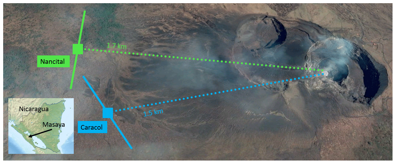
Figure 1Location and scan geometries of the NOVAC stations Caracol and Nancital at Masaya volcano. Coloured squares indicate the instrument location and solid lines the scan direction. For further parameters, see Table 1. The map was created with graphical material from https://commons.wikimedia.org/wiki/File:Nicaragua_relief_location_map.jpg (last access: 9 June 2021) and from © Google Earth.
Table 1Spatial set-up of the NOVAC stations at Masaya: altitude A, horizontal distance D to and angular orientation σ to the volcanic edifice, and orientation of the scan plane β (see Figs. 1 and 5).
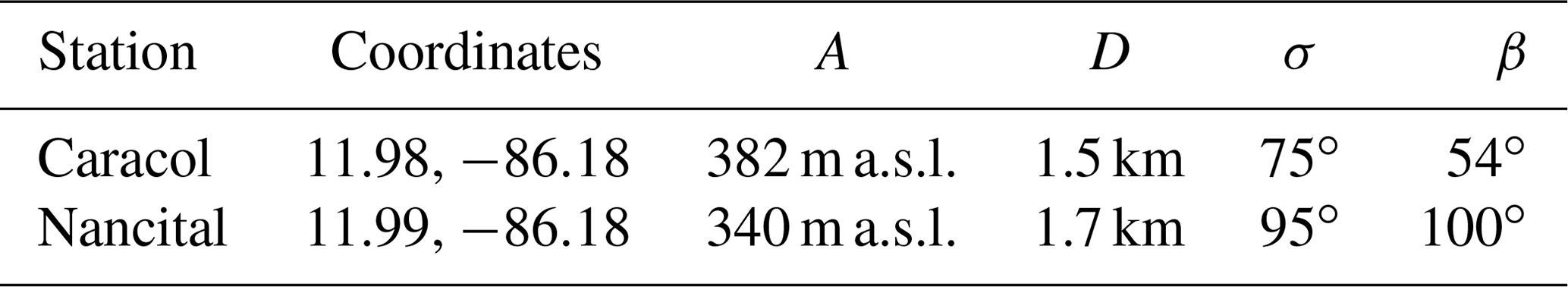

Figure 2Meteorological conditions at Masaya volcano retrieved from ECMWF ERA-Interim data with resolutions of 6 h and and interpolated to an altitude of 700 m a.s.l. Grey lines: 6-hourly data. Blue lines: running means over the 6-hourly data with an averaging window of ±7 d. Black dots: around-noon (18:00 UTC) data. Red lines: running means over the around-noon data with an averaging window of ±7 d. Absolute variations are almost the same for the full data set and the around-noon data only, except for the air temperature and the relative humidity, which follow their expected diurnal cycles.
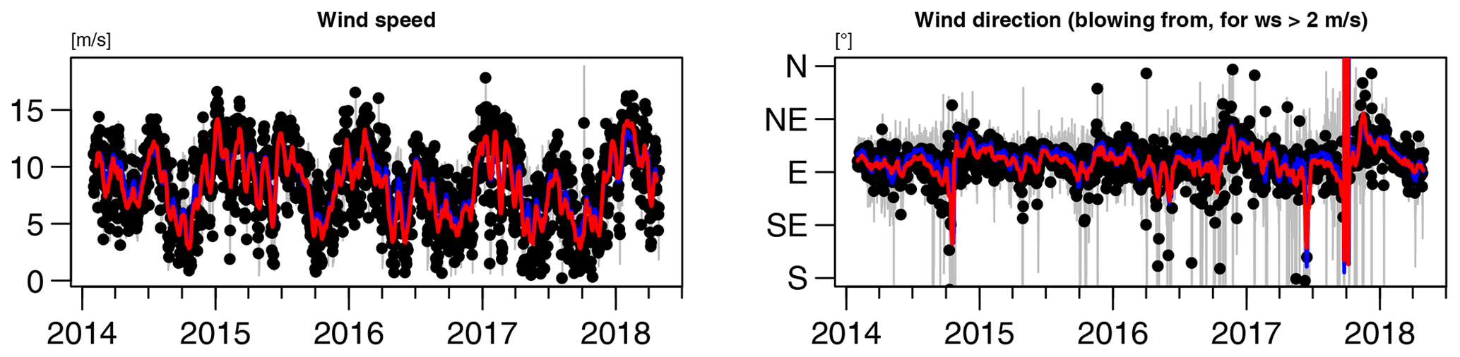
Figure 3Meteorological conditions at Masaya volcano retrieved from the operational ECMWF reanalysis data. See Fig. 2 for details.
2.1 ECMWF ERA-Interim data
The ECMWF ERA-Interim data set has an original spatial resolution of about (at and close to the Equator), a temporal resolution of 6 h (00:00, 6:00, 12:00, and 18:00 UTC), and 60 hybrid pressure layers which follow the terrain close to the ground and in the lower atmosphere and are constant in the higher atmosphere. They reach up to 10 Pa, i.e. about 66 km. The presented ECMWF data are vertically interpolated to an altitude of 700 m a.s.l. and horizontally gridded on a grid (i.e. about 110 km × 110 km at 12∘ N). The preparation of the ERA-Interim data on such a grid was chosen for in general better compatibility with other global data. For local studies, using the original data may be more appropriate, though this distinction becomes mostly obsolete due to our local calibration approach (see Sect. 3).
The following meteorological parameters are presented and discussed in this study: (1) the wind speed and (2) the wind direction in order to reconstruct the plume propagation direction, (3) the barometric pressure, (4) the ambient air temperature, (5) the water vapour concentration, (6) the relative humidity and (7) the ozone mixing ratio in order to investigate their possible influences on the plume chemistry, and (8) the total cloud cover (i.e. the fraction of the ground pixel area hidden from direct solar irradiation by visible clouds anywhere between ground and the top of the model domain) as a proxy for the radiative conditions.
The following quantitative discussion focuses on the 2-weekly moving average of ECMWF data around noon time, though a discussion of the unfiltered time series comes to similar results (see red and blue lines in Fig. 2). The time series exhibit annual cycles for all parameters, however, with different timing and spacing of their extrema and different significance of their amplitudes. The total cloud cover varied between two clearly distinguishable plateaus with mostly clear skies (values of 0.1±0.1) from December to March and predominantly dense coverage (values of 0.8±0.1) from May to October, indicating that Masaya is affected by the intertropical convergence zone (ITCZ) during that latter time interval. The wind speed varied between 3 and 17 m s−1, with maxima in January/February, weaker secondary maxima in July, and minima in June and in October. The average of the wind direction mainly indicates easterlies (75±28)∘ subject to an approximately linear trend each year with a step change each year towards east–northeasterly in October followed by an approximately linear trend towards easterly in September. In addition, the wind conditions are rather unstable each year in June and in October (which corresponds to the times when Masaya is located at the edge of the ITCZ). When those exceptions are ignored by limiting the set of wind directions to 40–110∘ (which contains 88 % of the raw data), the wind conditions were rather stable, with almost exclusively east–northeasterly winds from (75±10)∘ almost all of the year. The barometric pressure varied between 931 and 935 mbar, with weak minima in October/November. The ambient air temperature varied between 294 and 298 K, with maxima in April and minima in January. The water vapour concentration and the relative humidity varied between 4 and 6×10¹⁷ molec cm−3 and between 60 % and 90 %, respectively, with minima in February/March and maxima from June to October. The ozone mixing ratio varied between 20 and 50 ppbv, with minima usually around October and maxima in March.
2.2 Operational ECMWF reanalysis data
The accuracy of weather data, especially in the mountainous regions around the volcano, is directly related to the accuracy of the model topography. Therefore an enhanced (fundamental) model resolution should result in general in more representative data. For this purpose, we investigated the meteorological conditions at Masaya also by using the operational ECMWF reanalysis data with a higher spatial resolution of (modelled in the spectral domain with a truncation of T1279, interpolated to the Gaussian grid N640). The underlying model of the operational ECMWF reanalysis data is, however, updated frequently (e.g. since 8 March 2016 the model has used a finer horizontal resolution of 0.07∘ instead of 0.14∘), and thus there are potentially artificial jumps in its time series. Because this study analyses a long time series, a model set-up with such artificial changes is not suitable for direct application. A full list of modifications to the model set-up in addition to the change in horizontal model resolution can be found at https://www.ecmwf.int/en/forecasts/documentation-and-support/changes-ecmwf-model (last access: 9 June 2021).
2.3 Estimates for the wind speed and the wind direction
We based our analysis in general on the meteorological parameters from the ECMWF ERA-Interim data because this data set allows an analysis consistent in time, i.e. without potential jumps in the time series. Nevertheless, the ERA-Interim data have to be expected to provide only limited accuracy in particular in the complex topology around volcanoes. Therefore, we applied the following local calibrations of the ERA-Interim data.
We compared the wind speeds vera provided by the ERA-Interim data set and voad provided by the operational ECMWF reanalysis data. We consider the latter to be in general a more accurate estimate due to its higher spatial resolution. Despite the wind speeds from both data sets being highly correlated (coefficient of +0.89), their scatter plot deviates significantly from a proportional relationship. Instead,
is apparently a good fit (Fig. 7a). All wind speed data used in our further evaluation steps were retrieved from the ERA-Interim data but calibrated according to Eq. (1).
We consider the wind directions retrieved via the triangulation of the NOVAC results to be the “ground truth” (see Sect. 3). The operational ECMWF reanalysis data match well with these data, which further supports this assumption. The ERA-Interim data, however, provide wind directions which are further to the east–northeast by 11∘ (Fig. 7b). All wind direction data used in our further evaluation steps were retrieved from the ERA-Interim data but calibrated according to Eq. (2):
(the addition of 11∘ corresponds to a shift from east–northeasterly towards easterly).
These two calibrations could not be expected to improve the accuracy for every individual data point but result arguably on average in a more accurate data set.
We derived semi-continuous (only during daytime) time series of the differential slant column densities (dSCDs) of SO2 and BrO via multi-axis differential optical absorption spectroscopy (MAX-DOAS) applied to UV spectra of the diffuse solar irradiation recorded by the NOVAC stations (e.g. Edmonds et al., 2003; Galle et al., 2003; Bobrowski et al., 2003). The SO2 emission fluxes and the molar ratios in the volcanic plume were then derived from the dSCD data.
The spectroscopic retrieval of the SO2 and BrO dSCDs as well as the spectroscopic and post-spectroscopic retrieval of the molar ratios applied in this paper follow in large part the evaluation described by Dinger (2019), which itself follows mainly Lübcke et al. (2014) and Dinger et al. (2018).
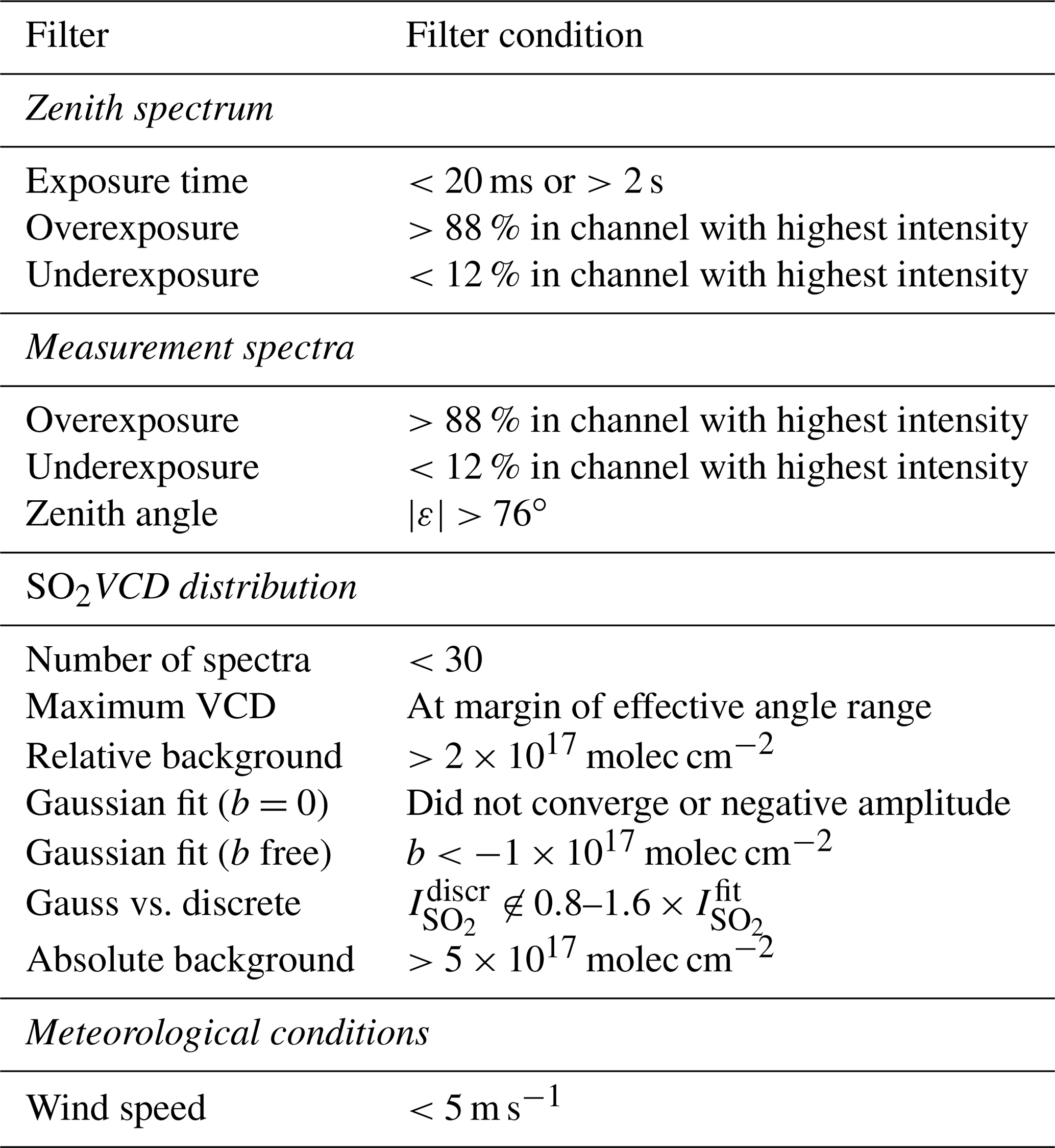
Our retrieval of the SO2 emission fluxes is based on the standard NOVAC approach described by Johansson et al. (2009) but (1) extended by a set of data filters which aim to reduce the amount of potentially problematic measurement conditions (see Table 2); (2) the spectroscopic retrieval was adapted to the high SO2 emission fluxes at Masaya, and (3) information on the plume height and the wind conditions was assessed partially via a triangulation of NOVAC observations. One of these filters uses the absolute SO2 background calibration method described by Lübcke et al. (2016).
Table 2Applied filters in chronological order (if condition fulfilled, reject data). See text for details. For comparison, the standard NOVAC retrieval applies the five following filter conditions (Johansson et al., 2009): (1) overexposure of (any) spectrum by more than 99 %, (2) underexposure of (any) spectrum by less than 2.5 %, (3) for a measurement spectrum, (4) number of passing spectra < 10, and (5) a “plume completeness filter” which rejects a scan if most of the large dSCDs are close to the margin of the effective angle range.
In this section, we describe the applied retrieval steps and data filters (see Table 2; further information on the retrieval can be found in Appendices B–D). A summary and critical assessment of our retrieval steps can be found in the discussion section of this paper.
3.1 Spectroscopic retrieval of the SO2 dSCD distribution
The NOVAC data were recorded by UV spectrometers which scan across the sky from horizon to horizon in steps of 3.6∘ by means of a small field-of-view telescope yielding a mean temporal resolution of about 5–15 min per scan. Each scan contains 53 spectra: an initial zenith spectrum, a dark current spectrum, and 51 measurement spectra (Galle et al., 2010).
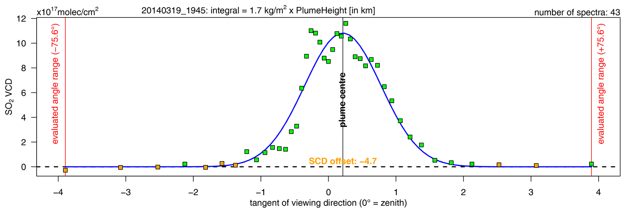
Figure 4SO2 VCD distribution retrieved from the scan starting at 19 March 2014 19:45 UTC recorded at Caracol station. The green and orange squares give the retrieved angular SO2 VCD distribution. Only data for zenith angles between −75.6 and +75.6∘ were considered. The orange squares were used for the retrieval of the background SCD (the set of the lowest SCDs does not necessarily match perfectly with the set of the lowest VCDs). The (negative) background SCD is given in orange. The plume centre is retrieved via the Gaussian fit (solid blue line).
Prior to the spectroscopic retrieval, the individual spectra of a scan were checked for their spectroscopic quality. A scan was rejected if its initial zenith spectrum was either overexposed or underexposed (accept only spectra whose channel with the highest number of counts has recorded within 12 %–88 % of the maximum possible count number, where only the lower boundary is assessed after the dark current correction) or the single exposure time was unreliable (less than 20 ms or more than 2 s). For a passing scan, all its measurement spectra were checked for overexposure or underexposure and individually rejected if necessary. Furthermore, all spectra recorded at scan zenith angles ε with ∘ were rejected in order to avoid large light paths or spectroscopic artefacts due to obstacles in the light path. Accordingly, at most 43 measurement spectra could pass the quality filters. A scan was entirely rejected if less than 30 of its spectra passed.
A remark on the overexposure filter: it was chosen as described above in order to ensure that BrO DOAS fits were not degraded by saturation effects. For the sole retrieval of the SO2 emission fluxes, it may be sufficient to check for overexposure exclusively in the SO2 fit range. Nevertheless, we aimed for the same database for both the molar ratios and the SO2 emission fluxes in order to ensure a consistent comparison of both time series. Further arguments for applying the overexposure filter on the overall spectrum are (1) that overexposure in the spectrum indicates significant variations in the intensity of the back-scattered solar radiations during a scan (caused presumably by variations in the cloudiness of the sky). Accordingly, the overexposure filter would (conveniently?!) reject those times with unstable meteorological conditions. (2) The saturation of any pixel of the charge-coupled device detector may cause the additional photo-electrons to spill over to other pixels and thus could lead to the degradation of the entire spectrum.
For every scan passing the quality filters, SO2 DOAS fits were applied to each of the passing spectra where the initial zenith spectrum of the respective scan was used as a reference spectrum (the DOAS fit scenarios are summarised in Table 3). The result was a distribution of SO2 dSCDs with respect to the zenith spectrum depending on the viewing direction. These SO2 distributions were used for three purposes: (1) the calculation of the SO2 emission fluxes, (2) the triangulation of the plume centre position for a retrieval of the plume height and the wind direction, and (3) the identification of the plume region in preparation for the retrieval.
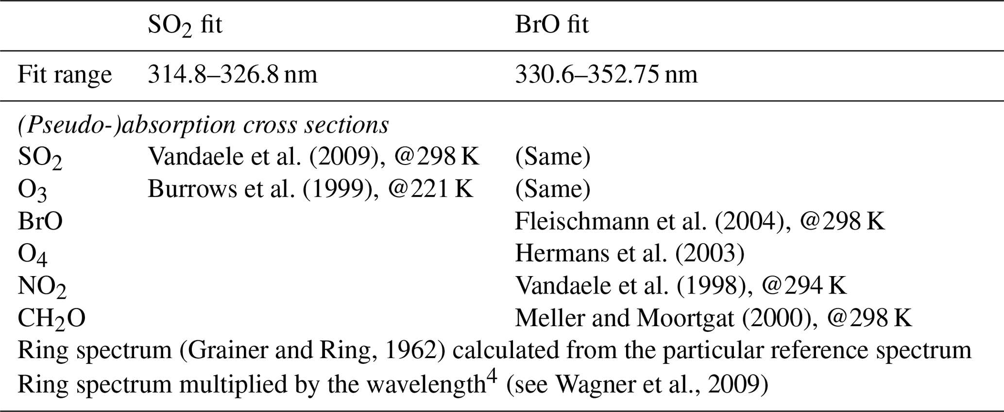
Vandaele et al. (2009)Burrows et al. (1999)Fleischmann et al. (2004)Hermans et al. (2003)Vandaele et al. (1998)Meller and Moortgat (2000)(Grainer and Ring, 1962)(see Wagner et al., 2009)Table 3Applied DOAS fit scenarios. The two lowest lines give the parameter ranges of the Levenberg–Marquardt fit routine. See Appendix B for the chosen wavelength range of the SO2 fit.
3.2 Retrieval of the background SO2 slant column density
The subsequent data analysis requires the absolute SO2 slant column density (SCD) distribution rather than the SO2 dSCD distribution, where . An accurate estimate for the absolute slant column density of the reference spectrum (here: of the initial zenith spectrum) is non-trivial. In the following, four different retrieval approaches are discussed (see Table 4). A pragmatic approach is the assumption that the scan included viewing directions which were not at all affected by a contamination with volcanic gases. This assumption would imply for the background direction εbg. In order to be less susceptible to negative outliers, we calculated as the mean of the eight lowest dSCDs (orange squares in Fig. 4).
Table 4Four different approaches for the retrieval of the background SO2 slant column density.

It has been observed, however, that the assumption of a non-contaminated background direction is not always justified (e.g. Lübcke et al., 2016). Another approach which does not rely on that assumption is the direct retrieval of via a SO2 DOAS fit of the zenith spectrum against a solar-atlas spectrum (see Salerno et al., 2009; Lübcke et al., 2016; Esse et al., 2020; Chance and Kurucz, 2010). This second approach requires, however, retrieval of the instrument characteristics (e.g. via a principal component analysis of the residual spectroscopic structure), which is not only a time-expensive procedure, but is also prone to introducing systematics when not carefully applied.
A third approach is the hybrid of these two approaches with the following subsequent steps: (1) apply the first approach to identify the viewing directions of the eight lowest SO2 dSCDs, (2) co-add these eight spectra, and (3) apply the second approach (i.e. evaluate against a solar-atlas spectrum) on this “added-reference spectrum” (instead of on the zenith spectrum; see Appendix C). In comparison to the pure second approach, the absolute retrieval step in this hybrid approach faces in general low – and mostly negligible – SO2 SCDs. Therefore, the SO2 DOAS fit of the absolute calibration retrieval can start at a wavelength of 310 nm or even lower (see also Appendix B), resulting in general in lower statistical fit errors and weaker effects from possible spectroscopic interferences of the SO2 absorption cross section with e.g. the imperfect estimation of the instrument characteristics. The results of the hybrid approach could be used either as a filter or for correcting the SCD data with respect to the retrieved background SO2 SCD.
A fourth approach extends the third approach by (1) checking for a background contamination but then (2) using a reference spectrum from another time (e.g. from the previous day at the same time) where a background contamination has been ruled out (e.g. via the second approach) for a subsequent iteration of the SO2 fits. Both the third and fourth approaches have in common that the chosen reference spectrum was not recorded under the same conditions as the measurement spectrum. The advantage of the fourth approach with respect to the third approach would be that the chosen reference spectra are expected to be recorded at least under similar conditions to the measurement spectra (at least when the time of day and the ambient temperature have been considered for the selection). The drawback of the fourth approach is the temporal variation of these systematics, while the third approach would cause the same systematics to all contaminated scans.
We applied the third approach to the data but used the results of the absolute calibration only for a rather conservative data filtering: we calculated the absolute background SO2 vertical column density (VCD) as the product of the absolute background SO2 SCD times the mean air mass factor mean(cos (εi∈bg)) but corrected by molec cm−2 for Caracol station and molec cm−2 for Nancital station (such that the peaks of the histograms match zero SO2; see Fig. 7c). A scan was rejected if its (corrected) absolute background SO2 VCD exceeded 5×10¹⁷ molec cm−2.
3.3 Calculation of the SO2 emission fluxes
The retrieval of the background SO2 SCD allows the calculation of the (absolute) vertical SO2 column densities
associated with the coordinates within the scan plane where the horizontal distance with respect to the instrument is H(ε)×tan (ε) and the mean plume height H(ε) (above the horizon of the instrument) can in general vary horizontally. We highlight that Eq. (3) assumes geometric air mass factors, while the real air mass factors could deviate due to angle-dependent atmospheric radiative transport effects (e.g. Mori et al., 2006; Kern et al., 2010). Examples of retrieved SO2 VCD distributions are shown in Figs. 4 and D3.
Precise information on the plume height is usually not available – not to mention spatially resolved variations of the plume height. A commonly applied pragmatic approach is thus the assumption of a plume height constant in space and time. Assuming that the plume height H(ε)=H is constant at least in space, the SO2 emission fluxes for a particular time can be calculated via
with the molar mass of SO2 g mol−1, the absolute wind speed v, and the relative angle between the wind direction and the scan plane (see Fig. 5). We highlight that the integral can be understood as a spatial integral which integrates along a straight horizontal line by steps of .

Figure 5Sketch of the geometric relations which are used to calculate the SO2 emission fluxes, to conduct the plume centre triangulation, and to estimate the plume age.
The angular integral d(tan (ε)) can be calculated in good approximation by a discrete summation of the spectroscopically retrieved SO2 VCD distribution via
where n is the number of all individual spectra (i.e. individual viewing directions) which passed the filters discussed above and Vi are the vertical SO2 column densities calculated according to Eq. (3) and associated with the horizontal coordinates H×tan (εi) as explained above.
Up to here, our methodology followed the standard NOVAC approach (Johansson et al., 2009). This approach tacitly assumes that the measurement conditions did not change significantly during one scan. This assumption could be frequently not justified due to several causes, e.g. unstable wind conditions or intra-minute variations in the volcanic degassing source strength (e.g. Pering et al., 2019). In the next paragraph, we present a set of filters which reject data which are potentially influenced by unstable measurement conditions. Afterwards, we present our approaches to estimate the wind conditions and the plume height.
3.4 Filtering of unstable conditions
For stable meteorological and radiative conditions as well as a constant SO2 emission strength, the horizontal broadening of a volcanic plume is caused predominantly by turbulent diffusion. Under such ideal measurement conditions, the SO2 VCD distribution would be a Gaussian distribution with respect to the distance (in the scan direction) H×tan (εi). A Gaussian shape is indeed observed in good approximation for a large part of the scans where exactly one plume has been identified (e.g. Figs. 4 and D3d). However, there is also a significant number of scans where the retrieved SO2 VCD distribution differs significantly from an ideal Gaussian shape. The predominant reason for such deviations is an apparent secondary plume (presumably either because there was another plume or because the wind direction changed during the scan), but less well-defined, rather random shapes were also observed (see Fig. D3a–c).
As motivated above, scans with unstable conditions should be rejected. We fitted a Gaussian distribution
as a function of tan (ε) to the SO2 VCD distribution (with the fit parameters a, μ, w, and b) as a tool to semi-quantitatively assess the “degree of stability” during that scan. In order to provide an automated test of the “Gaussian shape assumption”, we fitted two Gaussian distributions to the SO2 VCD distribution, one with a fixed b=0 and one with a free b (see the solid and dashed lines in Fig. D3, while both lines perfectly overlap in Fig. 4).
The Gaussian fits (and other criteria) were used to filter the data in six subsequent steps (F1)–(F6). A scan was rejected if: (F1) its highest SO2 VCD was retrieved at the margin of the effective angle range (which is usually at ±75.6∘) because in such a case at least half of the plume area was not included, (F2) the relative SO2 VCD background exceeded 2×10¹⁷ molec cm−2 because for stable conditions that offset should be non-positive by construction, and (F3) the Gaussian fit with fixed b=0 did not converge or proposed a negative amplitude (20 % and 5 % of the scans were rejected by these filters for Caracol station and Nancital station, respectively).
We highlight that the Gaussian fit would tend to propose a positive offset parameter b>0, e.g. if a secondary plume elevates the apparent background level. In contrast to that, significant negative values for b indicate that the effective scan range does not include the gas-free background. Accordingly, a scan was rejected if (F4) molec cm−2 (3 % and 1 % of scans rejected).
Next, we compared the Gaussian integral (retrieved for b=0) and the discrete integral . On the one hand, the Gaussian integral is also for b=0 usually smaller than the discrete integral (e.g. because of a secondary peak or an asymmetric plume shape). On the other hand, our filtering of data with ∘ implies the tacit assumption of Vi=0 for ∘ for Eq. (5). When this assumption does not hold true, the discrete integral underestimates the overall SO2 amount, while the Gaussian integral could correctly include those contributions. Therefore, a scan was rejected if its two integrals differed rather strongly; that is, a scan passed only if (F5) – (20 % and 10 % of scans rejected, with 12 % and 5 % due to the lower threshold and 8 % and 5 % due to the upper threshold). Furthermore, for a passing scan the higher value of the two integrals was chosen (where was chosen for 28 % and 23 % of the scans).
As a last filter (F6), a scan was rejected when its absolute SO2 background VCD exceeded 5×10¹⁷ molec cm−2 (see above; 8 % and 3 % of scans rejected).
In total, 57 % and 82 % of the scans passed the filters for Caracol station and Nancital station, respectively. We consider this a good compromise between the lack of temporal resolution and reducing the risk of systematic errors due to unstable measurement conditions.
3.5 Triangulation of the plume centre position
When the volcanic gas plume is observed simultaneously by two NOVAC stations (as was the case in the period from March to October 2014), the two associated viewing directions towards the plume centre can be used for a triangulation of the spatial position of the plume centre. The relationship between the plume height Hs above the horizon of the NOVAC station s and the wind direction ω is given by
where the fixed station geometry parameters A, D, σ, and β are summarised in Table 1 and the horizontal geometrical considerations are sketched in Fig. 5. We highlight that the total plume altitude Hs+As is the same for both instruments. If NOVAC station s observes εs=0∘, the wind direction is trivially given by ω=σs and the plume height can be retrieved by applying Eq. (7) to the other station.
We used the peak positions of the Gaussian fits introduced above (with b=0) as estimates for the plume centre position. A practical limitation of the triangulation was that the NOVAC stations did not measure exactly simultaneously. Therefore a temporal binning of their data was required. We calculated bins of 30 min. A bin was rejected if the plume centre varied for one instrument within these 30 min such that the standard deviation exceeded 20∘.
The plume centre triangulation proposed an average wind direction of (84±3)∘ and average total plume altitudes of m, which implied an average plume height above ground level of (378±94) m for Caracol station and (420±94) m for Nancital station (Fig. 6).
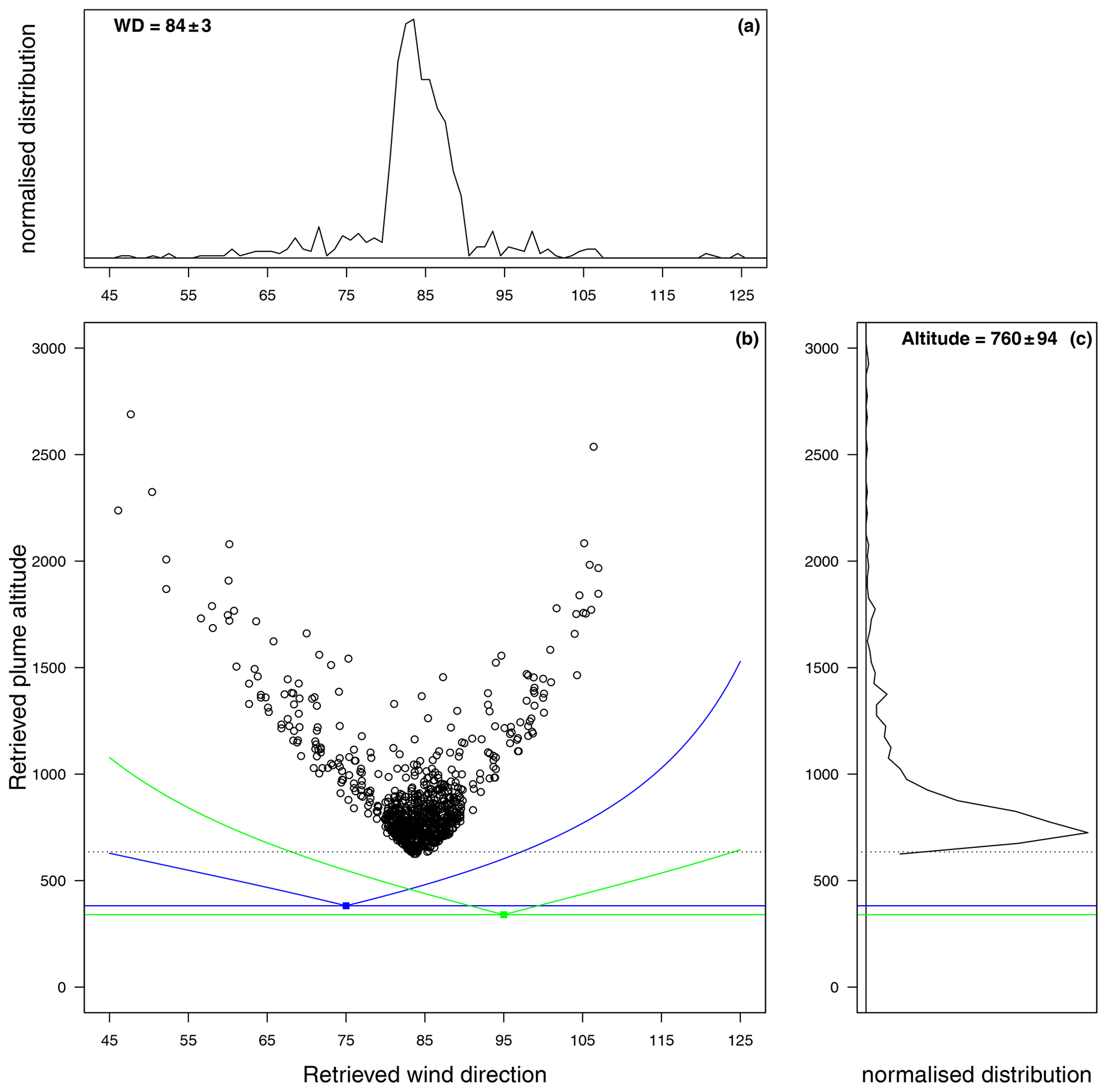
Figure 6Results of the plume centre triangulation. Data have been binned in 30 min intervals, and the means of the plume centre have been compared. A bin has been rejected if the plume centre varied for one instrument such that the standard deviation exceeded 20∘. (a) Histogram of the retrieved wind directions. (b) Scatter plot of the retrieved plume altitudes and the retrieved wind directions. The altitudes of Caracol and Nancital stations and of the volcanic edifice are marked by blue, green, and grey lines. The effective field of view ∘ of the two instruments is given by the curvy blue and green lines. The dominant bulk of observations centred at approximately (84∘, 756 m a.s.l.) refers to observations when both instruments nearly simultaneously recorded the sample plume, while the “wings” to the upper-left and upper-right corners refer to observation where both instruments recorded at the same time different plumes. The wings are presumably artefacts caused by the simplicity of the triangulation approach given in Eq. (7). (c) Histogram of the retrieved plume altitudes.
3.6 Estimates for the plume height
The plume altitude is a major source of uncertainty in the calculation of the SO2 emission fluxes. When lacking visual observations, the plume altitude is usually assumed to be fixed to the altitude level of the volcano summit or the expected effective plume height of the volcanic plume.
The plume height can be considered to vary significantly and depends on the wind conditions. The initial buoyancy of the volcanic plume is just one mechanism which links the plume height and the wind speed. The volcanic plume is usually hotter than the ambient atmosphere and thus rises until its temperature is equilibrated due to adiabatic cooling and mixing with ambient air. Accordingly, higher wind speeds should result on average in lower observed plume heights for at least two reasons: first, the higher the wind speed, the larger the atmospheric turbulence, the larger the cooling rate of the plume, and thus the lower the effective plume height. Second, the higher the (horizontal) wind speed was, the smaller has been the propagation time between release and observation, and thus the lower is the probability that the measured plume has already reached its effective plume height.
We tested this hypothesis with the triangulation results. For this test, we had to get rid of the artificial “wings” in the triangulation results (see Fig. 7). We realised this condition by considering only the 88 % of data below an retrieved plume altitude of 1200 m a.s.l. for the following analysis.
The comparison of the triangulated plume height with the wind speed (calibrated as explained above) confirmed such a causal link between the plume height and the wind speed (correlation coefficient of −0.28 when considering all wind speeds and of −0.25 when considering only wind speeds higher than 5 m s−1). We retrieved for the linear relationship of
a best fit (when Hs and As measured in metres and vcalibrated measured in m s−1) for m and s (when all wind speeds were considered, F statistics of 64.7, p value = ) or m and s (when only wind speeds higher than 5 m s−1 were considered, F statistics of 41.6, p value = ).
As a remark, we also retrieved similarly well-matching fits for a quadratic relationship of
with a best fit for m and s2 m−1 (when all wind speeds were considered, F statistics of 64.8, p value = ) and m and s2 m−1 (when only wind speeds higher than 5 m s−1 were considered, F statistics of 38.9, p value = ).
We chose to use the linear relationship retrieved for wind speeds higher than 5 m s−1 for dynamic estimates of the plume height as a function of the wind speed; i.e. we applied a Hs retrieved via
as the estimate for the plume height in the calculation of the SO2 emission fluxes.
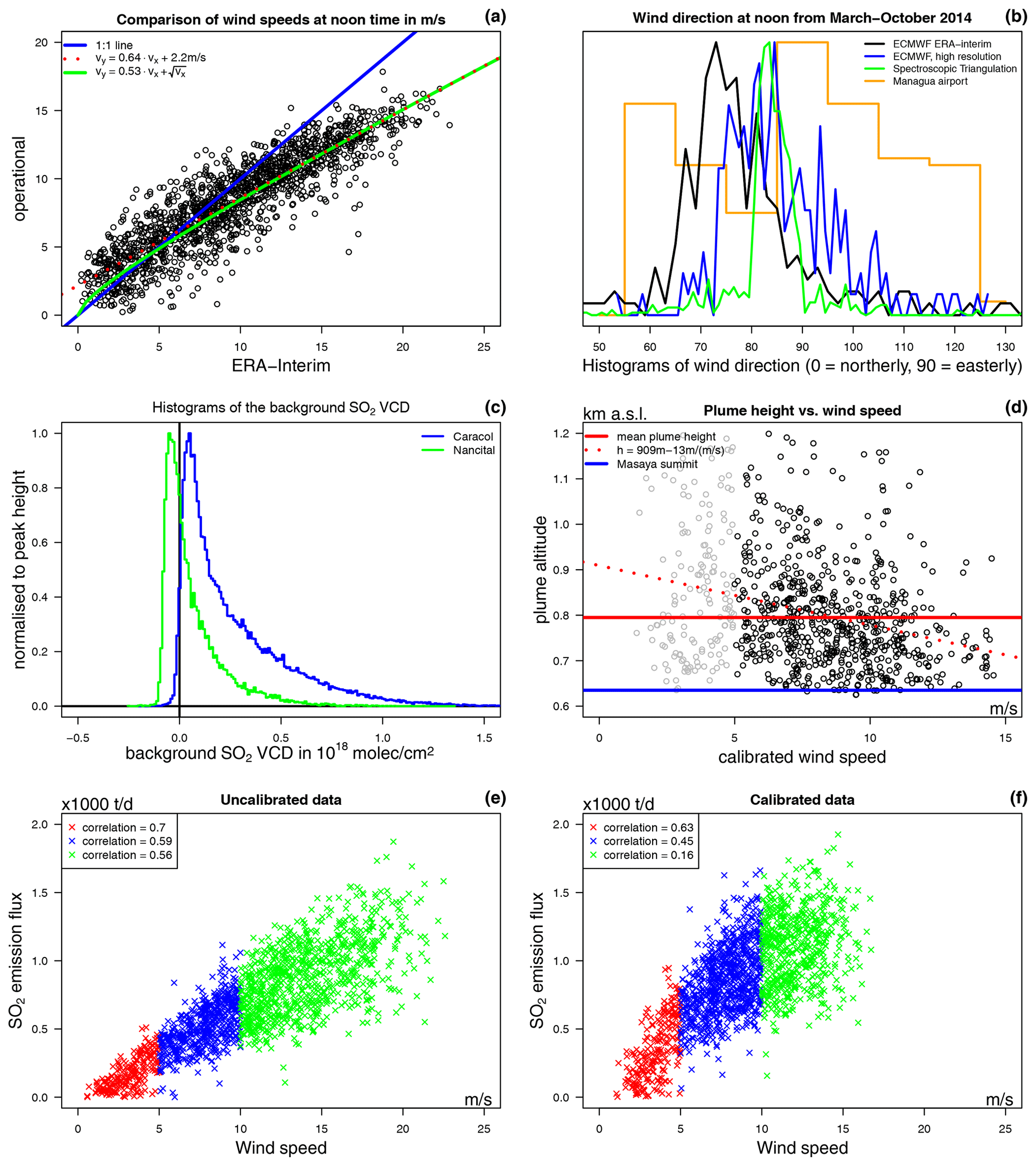
Figure 7Summary of several empirical observations used for filtering and estimations. (a) Comparison of the wind speeds from the ECMWF ERA-Interim data and the operational ECMWF reanalysis data. (b) Comparison of the distribution of the wind directions estimated by four different methods. (c) Histograms of the absolute SO2 SCD of the background spectrum for both instruments for their respective total time series. (d) Scatter plot of the triangulated plume height and the calibrated wind speed. The red dotted line indicates the relationship between wind speed and plume height (fit based on the black circles). (e, f) Correlation between the retrieved SO2 emission fluxes and the wind speed. The plots compare daily SO2 means and the means of the wind speed at the respective measurement times. (e) Original ERA-Interim wind speeds versus the non-calibrated SO2 emission fluxes calculated with original ERA-Interim wind conditions and a fixed plume altitude of 635 m a.s.l. (f) Calibrated wind speeds versus the SO2 emission fluxes calculated with the calibrated wind conditions and a dynamic plume altitude as a function of the wind speed.
We are aware that this relationship is subject to a large scatter, though we consider it a better best guess than applying a fixed plume height. In particular, using a fixed plume height could result in apparent seasonal variations in the SO2 emission fluxes which are, however, possibly only inherited artefacts due to seasonal variations of the wind speed (see next paragraph).
3.7 (Apparent) correlation of SO2 emission fluxes and wind speeds
We initially observed a strong correlation between the SO2 emission fluxes and the wind speeds when none of our estimation approaches for the wind speed, the wind direction, or the plume height were applied (correlation coefficient of +0.84 when all wind speeds are considered and of +0.56 when only wind speeds higher than 10 m s−1 are considered, Fig. 7e). This correlation was lower for the calibrated data (correlation coefficient of +0.71 when all wind speeds are considered) and in particular basically vanished for wind speeds higher than 10 m s−1 (correlation coefficient of +0.16, Fig. 7f). The SO2 emission fluxes are of magmatic origin, and thus no causal link to the meteorological conditions would be expected.
For March–October 2014, the SO2 emission fluxes can be calculated alternatively via the triangulation results, i.e. using the triangulated plume height and plume propagation direction instead of the parameterised plume height and the wind direction from ECMWF. We calculated the SO2 emission fluxes accordingly while using only data with triangulated plume altitudes below 1200 m a.s.l. in order to be consistent with the parametrisation approach explained above (and again in order to avoid the influence of the artificial “wings”). For these alternative SO2 emission flux estimates, the correlation between the SO2 emission fluxes and the wind speeds was significantly lower and completely vanished for wind speeds higher than 10 m s−1 (correlation coefficients of +0.05 and +0.02 for the two NOVAC stations; see Fig. D1).
We conclude that the observed correlation between the SO2 emission fluxes and the wind speed is rather not a real observation but is more likely caused by inaccurate SO2 emission fluxes and in particular by neglecting the variations in the plume height. For better readability, we postponed a more detailed discussion of this observation to Sect. 5 “Discussion of the SO2 emission flux retrieval”.
On the one hand, our proposed calibrations were able to correct this spurious correlation for wind speeds higher than 10 m s−1 (Fig. 7f). On the other hand, we were not able to explain or correct for that correlation for wind speeds lower than 10 m s−1. Accordingly, it could be appropriate to reject all data with wind speeds smaller than 10 m s−1, but this would massively reduce our data set (this would reject 72 % and 78 % of the remaining scans for Caracol and Nancital stations, respectively). As a compromise between data reliability and temporal resolution, we thus applied a more conservative filter and reject only those data with wind speeds smaller than 5 m s−1. This subsequent filter rejected 15 % and 22 % of the remaining scans for Caracol and Nancital stations, respectively.
3.8 Retrieval of the molar ratios
When retrieving BrO column densities in a volcanic gas plume from DOAS measurements, the expected optical depth of BrO absorption bands is at least 1 order of magnitude smaller than for SO2. Thus, a better photon statistic is required for sufficiently precise BrO results beyond the detection limit. At manually controlled measurements, this is often realised by averaging over a sufficiently large number of consecutive exposures (and besides, typical state-of-the-art campaign DOAS instruments are much more precise than NOVAC instruments due to better spectrometers and an active temperature stabilisation; see e.g. Kern and Lyons, 2018). For NOVAC data optimised with respect to the SO2 retrieval requirements, the required larger number of exposures per spectrum can be realised by a subsequent co-adding of multiple spectra which are recorded in temporal proximity and in the same or at least a similar viewing direction.
For this purpose, the retrieved SO2 dSCD distribution was used to identify all spectra which were predominantly part of the volcanic plume, and then these spectra were added in order to get one “added-plume spectrum” per scan. Analogously, the spectra which were associated with the 10 lowest SO2 dSCDs were added in order to get one “added-reference spectrum”. The drawback of this approach is the loss of spatial information because the retrieval derives only 1 averaged value for the BrO dSCDs and thus for the molar ratios. Accordingly, this approach does not allow us to investigate possible variations of the molar ratio as a function of e.g. the distance to the plume centre.
As mentioned above, a volcanic gas plume can be expected to have an approximately Gaussian-shaped angular gas distribution embedded in a flat, gas-free reference region. Therefore we fitted a Gaussian distribution to the SO2 dSCD distribution as a function of the zenith angles. The standard deviation range of the Gaussian distribution (αpeak±σGauss) was then defined as the plume region. The applied filters of the retrieval were less strict than for the SO2 emission flux retrieval: a scan was rejected from the further analysis only if the Gaussian fit failed to converge or if σGauss<5∘. Furthermore, if σGauss was rather large, the such defined plume region may have overlapped with the reference region. To avoid this inconsistency, we implemented the following procedure: if the derived (Gaussian) plume region included more than 10 spectra, the plume region was instead defined as the angle range with the highest running mean value over 10 spectra for the SO2 dSCD. The spectra associated with the plume region were spectroscopically added to a single “added-plume spectrum”.
We highlight that it would be more consistent to fit the Gaussian distribution to the SO2 VCD distribution as a function of the tangent of the zenith angles (instead of a fit to the SO2 dSCD distribution as a function of the zenith angles). Nevertheless, the maximum possible effect would be that the ±1 spectrum is included in the plume region. We used the fit in the dSCD–angle space for practical and historical reasons but, in the future, would encourage fitting in the VCD–tangent space instead for maximum consistency with the SO2 flux retrieval.
The added-plume spectra and added-reference spectra per scan were used for a second iteration of the spectroscopic retrieval in order to retrieve SO2 and BrO dSCDs representative of the plume centre. From this set of scans, all scans with sufficiently reliable BrO fits (here: scans with a fit quality of ) were used for a third iteration: the added-plume spectra and added-reference spectra of four consecutive scans were added, and again SO2 and BrO DOAS fits were applied. An I0 correction was applied to these final data (Platt and Stutz, 2008), which had not been done beforehand in order to save evaluation time.
The SO2 and BrO dSCDs and the molar ratios discussed in this paper refer to the results of the third spectroscopic iteration (Fig. 8). We highlight that these dSCDs are not absolutely calibrated for a background contamination (see above) because no reliable method for a absolute calibration of a background contamination with BrO has been developed (in contrast to the SO2 retrieval). The interpretation of the molar ratios thus tacitly assumes that a possible background contamination has the same molar ratio as the main plume. For the first investigations of this assumption and possible advances towards a correction of a BrO contamination, see Wilken (2018).
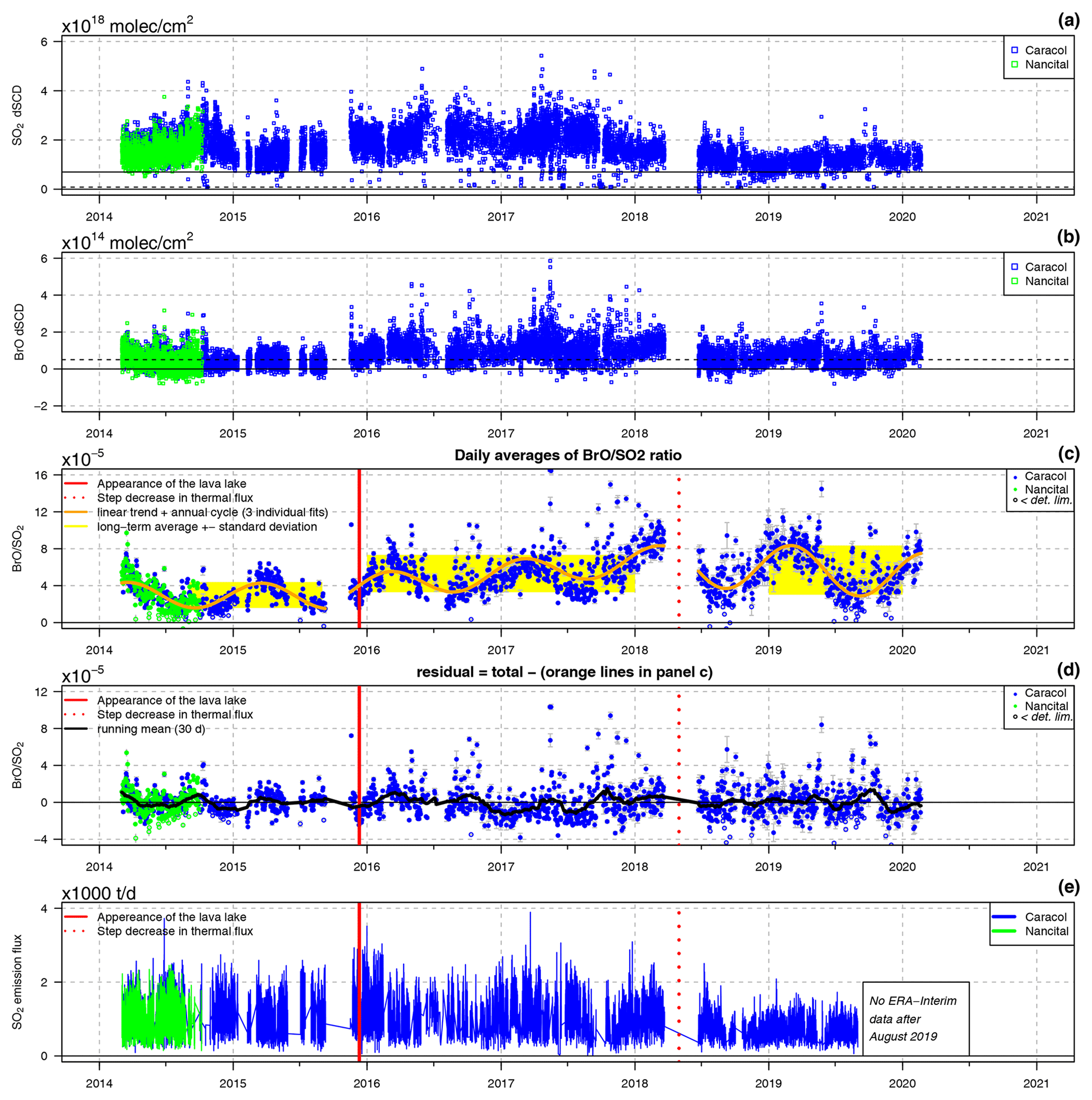
Figure 8(a–c) Time series of the differential slant column densities of SO2 and BrO and calculated daily means of the molar ratios in the gas plume emitted from Masaya (long/short tick marks indicate 1 January/July). The two NOVAC stations are indicated by the different colours. (c) Best fits of the long-term pattern are given for three individual time intervals (orange lines). The yellow bands indicate the long-term averages and the standard deviations. (d) Residual time series when subtracting the best fits from the three individual parts of the time series. e) Daily means of the SO2 emission fluxes.
We highlight that the retrieval of the molar ratios is hardly affected by the numerous potential sources of systematic effects, as is the case for the SO2 emission fluxes. For instance, the molar ratio is not affected by assumptions about the air mass factor and about the plume height. In addition, when BrO and SO2 are retrieved from similar wavelength regions, the molar ratio appears to be hardly susceptible to systematic effects in the radiative transport, because then the quantitative effects are similar for BrO and SO2 and thus cancel in good approximation (Lübcke et al., 2014).
In this section, we present the SO2 and BrO time series retrieved from the NOVAC data. There were two major data gaps in the NOVAC time series from 9 September to 16 November 2015 and from 21 March to 23 June 2018. The statistical analysis results discussed in the following, therefore, refer to the time intervals (1) March 2014–September 2015, (2) November 2015–March 2018, and (3) June 2018–March 2020.
This separation into three time series is also in good agreement with the three episodes of general volcanological observations of the lava lake activity: (1) “prior to the lava lake appearance (until November 2015)”, (2) “period of high lava lake activity” (from November 2015 to October 2018, where the thermal activity started at the latest on 15 November and the lava lake visualised on 15 December; INETER, 2015a, b; Aiuppa et al., 2018), and (3) “period of low lava lake activity (from October 2018 on)” (Global Volcanism Program, 2018). It has been reported that Masaya was already relatively calm before May 2018 (Global Volcanism Program, 2018), indicating that the major transition from high to low activity may have happened sometime during the data gap from March to June 2018. The minor discrepancy in separation with respect to the time span from June to October 2018 was not elaborated on in our study.
The long-term averages of these time intervals were retrieved for intervals spanning exact multiples of a year in order to avoid biases due to the seasonal modulation, namely 1 September 2014–1 September 2015, 1 January 2016–1 January 2018, and 1 January 2019–1 January 2020.
4.1 SO2 and BrO dSCDs
The data from Caracol station and Nancital station were in general in good agreement (correlation coefficients of +0.82 and +0.77 for daily averages of SO2 and BrO dSCDs). Caracol station observed on average higher dSCDs with relative factors of 1.18±0.21 for SO2 and 1.06±0.24 for BrO (when neglecting data with BrO dSCDs below 5×10¹³ molec cm−2, as these were deemed too close to the instrument detection limit). Analogously, relative factors of 1.12±0.20 and 0.99±0.19 were observed for the daily averages of the SO2 emission fluxes (see Sect. 5 and Fig. 9) and of the molar ratios, respectively.

Figure 9Comparison of the SO2 emission flux estimates when both NOVAC stations observed volcanic plumes within the same time bin of hourly means (grey triangles) and daily means (black circles). The plot compares the bin averages, and only data for wind speeds higher than 5 m s−1 were considered.
In the following, we discuss the typical variations observed by Caracol station. From March 2014 to September 2015, the SO2 dSCDs varied between 1 and 3×10¹⁸ molec cm−2, and the BrO dSCDs had daily maxima of about 1.5×10¹⁴ molec cm−2 but with peaks of up to 3×10¹⁴ molec cm−2. From November 2015 to March 2018, the SO2 dSCDs varied predominantly between 1 and 4×10¹⁸ molec cm−2 but with 9 % of the data varying between 4 and 8×10¹⁸ molec cm−2, and the BrO dSCDs doubled with daily maxima of about 3×10¹⁴ molec cm−2 with peaks of up to 6×10¹⁴ molec cm−2. From June 2018 to March 2020, the SO2 dSCDs were lower again and varied between 1 and 2×10¹⁸ molec cm−2, and the BrO dSCDs had daily maxima of about 1.5×10¹⁴ molec cm−2. In summary, for the second time interval the SO2 and BrO dSCDs time series showed enhanced long-term averages but also a significantly larger variability.
Furthermore, a Lomb–Scargle periodicity analysis indicated that the SO2 dSCDs followed an annual cycle with pronounced minima during January of each year (false alarm probability of ) and that the BrO dSCDs followed an annual cycle () with an additional semi-annual modulation ().
4.2 Patterns in the time series
Considering the whole time series from 2014 to 2020, the average molar ratios were and subject to characteristic variations between 1 and . The molar ratios strongly differed between the three periods of volcanic activity, with average molar ratios of , , and (see yellow bars in Fig. 8c).
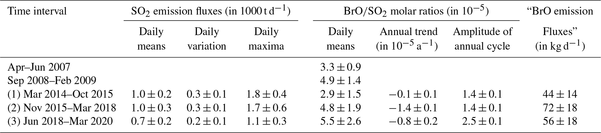
In addition to the variations described in the previous section, the time series indicated an annual cycle with maxima in early March accompanied by a semi-annual modulation (indicated by a Lomb–Scargle analysis, false alarm probability of ) as well as a varying long-term trend. These patterns were investigated for each of the three time intervals separately by fitting linear trends plus a sinusoidal variation with a period of 1 year to the respective time series. All fits were significant, with p values < , and the same holds for all individual regressors if not stated differently. For all three time intervals the phase of the annual cycle remained basically the same, but the average amplitude of the cycle varied between the three time intervals, being , , and , respectively. The accompanying linear trends in the time series were (p value = 0.48), , and per year for the three time intervals (see Table 5). An extrapolation of the trends of the two earlier time intervals to 11 December 2015, which is the date of the lava lake appearance, implied an apparent step increase by in the average molar ratios.
Table 5Main statistical properties of the spectroscopic results for Caracol station. Early NOVAC observations between 2007 and 2009 are listed for completeness. The daily variations are based on the standard deviations of the single days. The given errors are standard deviations, except for the annual trend and the amplitude of the annual cycle for the molar ratios where the errors refer to the standard regression error.
The residual patterns were investigated by subtracting the fitted variations (annual cycle and trend) from the respective time series for the three time intervals. Most residual variations spanned between subject to a standard deviation of and some outliers of up to (Fig. 8d). A Lomb–Scargle periodicity analysis indicated a weak semi-annual modulation with an amplitude of of the dominant annual periodicity with maxima in each March and September (false alarm probability of ).
4.3 SO2 and minimum bromine emission fluxes
For Caracol station separated for the three time intervals, (a) the mean daily averages of the SO2 emission fluxes, (b) the average daily variability, and (c) the averages of the daily maximum SO2 emission fluxes are listed in Table 5. From March 2014 to March 2018, the daily means of the SO2 emission fluxes were in general constant at t d−1, with the exception of December 2015–February 2016 (i.e. in the 3 months after lava lake appearance), when they were enhanced at t d−1. Furthermore, a Lomb–Scargle analysis indicated a weak semi-annual cyclicity in the SO2 emission fluxes (false alarm probability of ). The product of the SO2 emission fluxes and the molar ratios allowed the calculation of the apparent BrO emission fluxes (with the molar masses Mi). The according apparent BrO emission fluxes would be 44, 72, and 56 kg d−1 for the three time intervals. The apparent BrO emission fluxes multiplied by can be considered lower limits for the total bromine emission fluxes, because not all emitted bromine would have been transformed into BrO. According to model studies, the total bromine emissions would likely have been at least a factor of 2 larger than the derived apparent BrO emission fluxes (von Glasow, 2010; Roberts et al., 2014).
5.1 Intrinsic uncertainty in the SO2 emission fluxes
The simultaneous observation of basically the same volcanic gas plumes by two close NOVAC stations was a rare opportunity to retrieve empirically the lower limit of the uncertainty of the SO2 emission fluxes. For ideal measurements, both stations would observe identical SO2 emission fluxes, but under real measurement conditions systematic as well as statistical deviations can be expected.
It is important to note that the two stations usually did not record exactly the same plume, but their telescopes pointed at different times to the volcanic plume, with time differences of several minutes between their “simultaneous” observations. Pering et al. (2019) reported for SO2 camera measurements at the crater rim that the SO2 emission fluxes frequently vary by more than 100 % within minutes. We observed a similar variability when we analysed the SO2 emission fluxes retrieved by the two stations, with only several minutes between their observations. Accordingly, the higher the temporal resolution of the compared data, the larger the expected scatter of the comparison.
We calculated the ratios (called “relative factors” in the following) of the SO2 emission fluxes retrieved by Caracol station divided by the SO2 emission fluxes retrieved by Nancital station using several temporal bin sizes. The relative factor and standard deviation of the scatter were 1.22±0.55 for a 10 min binning, 1.19±0.40 for a 1 h binning, 1.13±0.21 for daily means, and 1.11±0.15 for weekly means (the 1-hourly data and the daily means are shown in Fig. 9). Our observations confirmed the significant reduction in the scatter with increasing bin size. In contrast to that, we observed a rather persistent relative factor of 1.1–1.2 for all bin sizes, with nevertheless a weakly decreasing trend as a function of the bin size.
The observed relative factor of 1.13 for daily means is relatively small in view of the uncertainties in the estimates of the meteorological conditions but also other measurement uncertainties. There are four obvious candidates for effects which may have contributed to the deviation of that factor from unity: (i) wrong geometric parameters of the NOVAC stations, (ii) misestimations of the wind direction or the plume height, (iii) systematic deviations in a possible underestimation of the SO2 dSCD, and (iv) radiative transport effects.
- i.
The most mundane cause of the observed offset would be wrong information on the viewing directions of the telescopes of the NOVAC instruments. For instance, with respect to a wind direction of 84∘ a variation of the scan plane orientation β by ±15∘ would result in a systematic miscalculation of the SO2 emission fluxes by a factor of 0.92–1.01 for Caracol station or 0.92–1.02 for Nancital station, i.e. up to a relative factor of 1.11. Analogously, a misalignment of the zenith angle by as little as ±5∘ can cause a systematic miscalculation of the VCDs (and thus the SO2 emission fluxes) by a factor of 0.9–1.1 when the volcanic plume is observed at ±50∘. If both stations are affected, such apparently negligible misalignments of the zenith angle can cause a relative factor of about 1.2 between both stations.
- ii.
A misestimation of the plume altitude can not only result in an absolute misestimation of the SO2 emission fluxes, but can also contribute to the observed relative factor because the stations are installed at different altitudes. For instance, and for the particular conditions at Masaya, using a mean plume altitude of 1000 m a.s.l. instead of 635 m a.s.l. would cause a relative factor of 1.09.
- iii.
A more subtle source for the observed relative factor and scatter could be the relation between an underestimation of the SO2 VCD and the absolute zenith angle: given a fixed SO2 VCD, the larger the absolute zenith angle, the larger the observed SO2 dSCD and thus the larger the probability of a significant underestimation of the SO2 VCD. Accordingly, if one of the instruments records shallow plumes systematically more often than the other instrument, this instrument would thus retrieve systematically lower SO2 emission fluxes. Both instruments, nevertheless, observed the volcanic plumes on average at the same (absolute) zenith angles, and thus this possible candidate appears to be irrelevant here.
- iv.
There could be significant deviations in the SO2 emission fluxes recorded by the two stations due to different radiative transport effects. For Masaya, the radiative transport effects associated with the relative position of the Sun were, however, presumably rather similar for both NOVAC stations because for March–October the Sun was for most of the day close to the zenith. Relative differences in the radiative transport caused e.g. when there were systematically more clouds either to the north or the south of the NOVAC stations could nevertheless not be ruled out as a source of the relative factor deviating from unity.
5.2 Correlation of SO2 emission fluxes and wind speeds
We observed a strong correlation between the SO2 emission fluxes and the wind speeds when none of our correction approaches for the wind speed, the wind direction, or the plume height were applied (correlation coefficient of +0.84 when all wind speeds are considered and of +0.56 when only wind speeds higher than 10 m s−1 are considered, Fig. 7e). This correlation was lower for the calibrated data (correlation coefficient of +0.71 when all wind speeds are considered) and in particular basically vanished for wind speeds higher than 10 m s−1 (correlation coefficient of +0.16, Fig. 7f).
The SO2 emission fluxes are of magmatic origin, and thus no causal link to the meteorological conditions would be expected. There are three groups of possible causes of this observation: (1) a chance coincidence of shared long-term patterns (e.g. an annual cyclicity), (2) causal links between the wind speed and the “volcanic” (in contrast to “magmatic”) gas emission flux, and (3) a systematically wrong calculation of the SO2 emission fluxes. In the following the plausibility of these options is discussed.
-
The wind speed followed a semi-annual cyclicity with strong maxima in January/February and weaker maxima in July. If the observed correlation was caused by a chance coincidence, this would imply an annual cyclicity in the volcanic degassing behaviour with maxima in January/February. Such an annual cycle could e.g. be caused by an astronomical forcing. The two best candidates, the solar irradiance and the Earth tidal potential, are indeed at Masaya minimum in December/January and June/July. Nevertheless, it is still far from obvious that these forcings can cause such a strong annual modulation of the SO2 emission flux.
-
There is indeed a plausible mechanism which links the wind speed and the SO2 emission flux: volcanic gas emissions often accumulate in the crater of Masaya. The larger the wind speed, the higher the atmospheric turbulence and thus the lower the accumulation. Accordingly and if the wind speed is subject to significant short-term fluctuations, over-proportionally much volcanic gas gets effectively released from the volcanic edifice into the atmosphere during high wind speed peaks. However, the observed correlation is based on long-term variations in the wind speeds but not on short-term fluctuations. While the temporal variability of our SO2 time series could be partially caused by this mechanism, our wind data (with a temporal resolution of 6 h) are insensitive to short-term effects, and that causal link can be ruled out as a cause of the observed correlation. We highlight that this mechanism may partially explain the high variability in the SO2 emission fluxes as observed by Pering et al. (2019).
-
There are a number of possibilities how the observed correlation could be caused by systematic effects in the retrieval of the SO2 emission fluxes: the plume height estimate could systematically depend on (a) the wind speed, (b) the SO2 emission flux, (c) the retrieval of the background SO2 SCD, or (d) an observational bias caused by the applied filters.
- a.
As discussed above, we expected and indeed observed a weak anti-correlation between the plume height and the wind speeds (Fig. 7d), which can explain the observed correlation for wind speeds higher than 10 m s−1 (Fig. 7f). We therefore conclude that this mechanism is one of the predominant causes of the observed correlation.
- b.
The stronger the absolute volcanic gas emission fluxes (i.e. in particular of H2O), the slower the cooling of the volcanic plume due to in-mixing of air and thus the higher the effective plume height of the buoyant gas plume. Combined with the general expectation that the wind speed is larger with increasing height above ground, we conclude that the higher the SO2 emission flux (when assuming that it is proportional to the absolute gas emission flux), the higher the wind speed at plume propagation altitude. Using only wind speeds for a fixed altitude level to calculate the SO2 emission fluxes, we can then expect an anti-correlation between the SO2 emission flux estimates and the applied wind speed.
- c.
Lübcke et al. (2016) reported for Nevado del Ruiz and Tunguragua that the probability of the clear-sky reference spectrum being contaminated with SO2 is higher for low wind speeds. Thus, at low wind speeds the SO2 SCD (and hence the SO2 emission flux) is more likely to be underestimated than at high wind speeds. Nevertheless, applying our method for removing SO2 contaminated references had practically no effect on the correlation of emission rate and wind speed, thus indicating that background contamination was not a major cause of the observed correlation.
- d.
The more strongly the observed plume shape deviates from an ideal Gaussian shape, the larger the probability that the scan will be rejected from the applied data filters. The plume shape is arguably better confined for larger wind speeds because then the relatively short time interval prior to the observation implies a smaller horizontal plume dispersion. Nevertheless, we would neither expect nor did some data checks support the assumption that such observational biases could have caused the observed correlation.
- a.
5.3 Comparison with reported SO2 emission fluxes
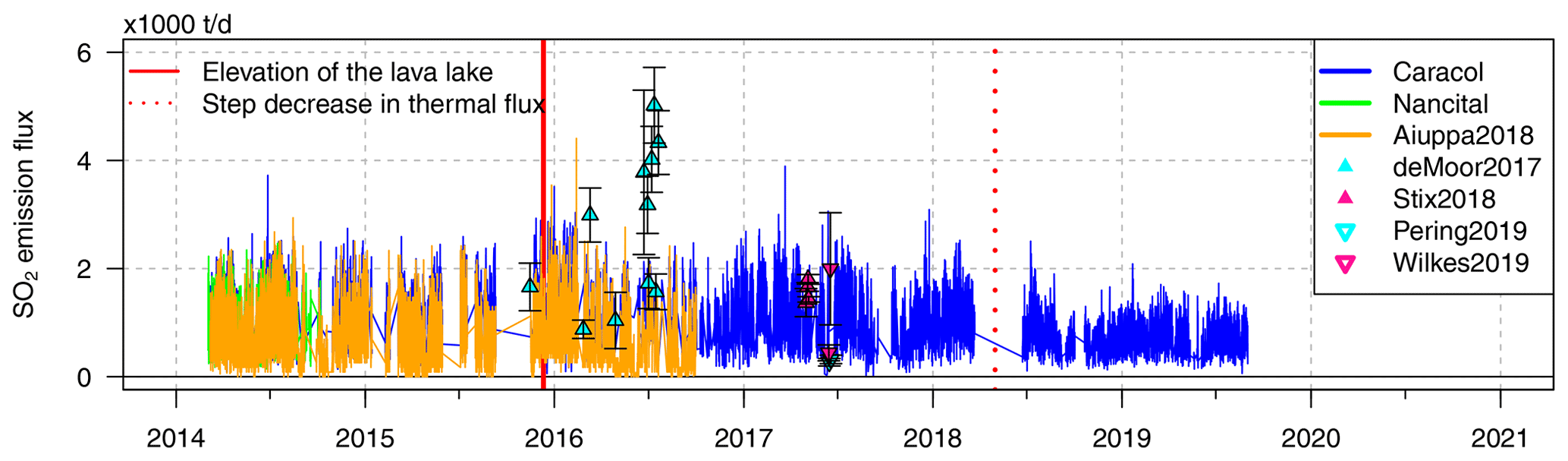
For 2014–2017, Aiuppa et al. (2018) retrieved from the same NOVAC data and ERA-Interim data mean SO2 emission fluxes of (700±400) t d−1 subject to variations between 0 and 2600 t d−1 (Fig. 10). Our and their SO2 time series show a good agreement in relative variability, but we observed considerably higher values with average relative factors of 1.42±0.46 (Fig. 11). This relative factor can be explained by the combination of the deviations in (1) the SO2 dSCD retrieval, (2) the plume height estimates, and (3) the wind speed estimates, as detailed in the following.
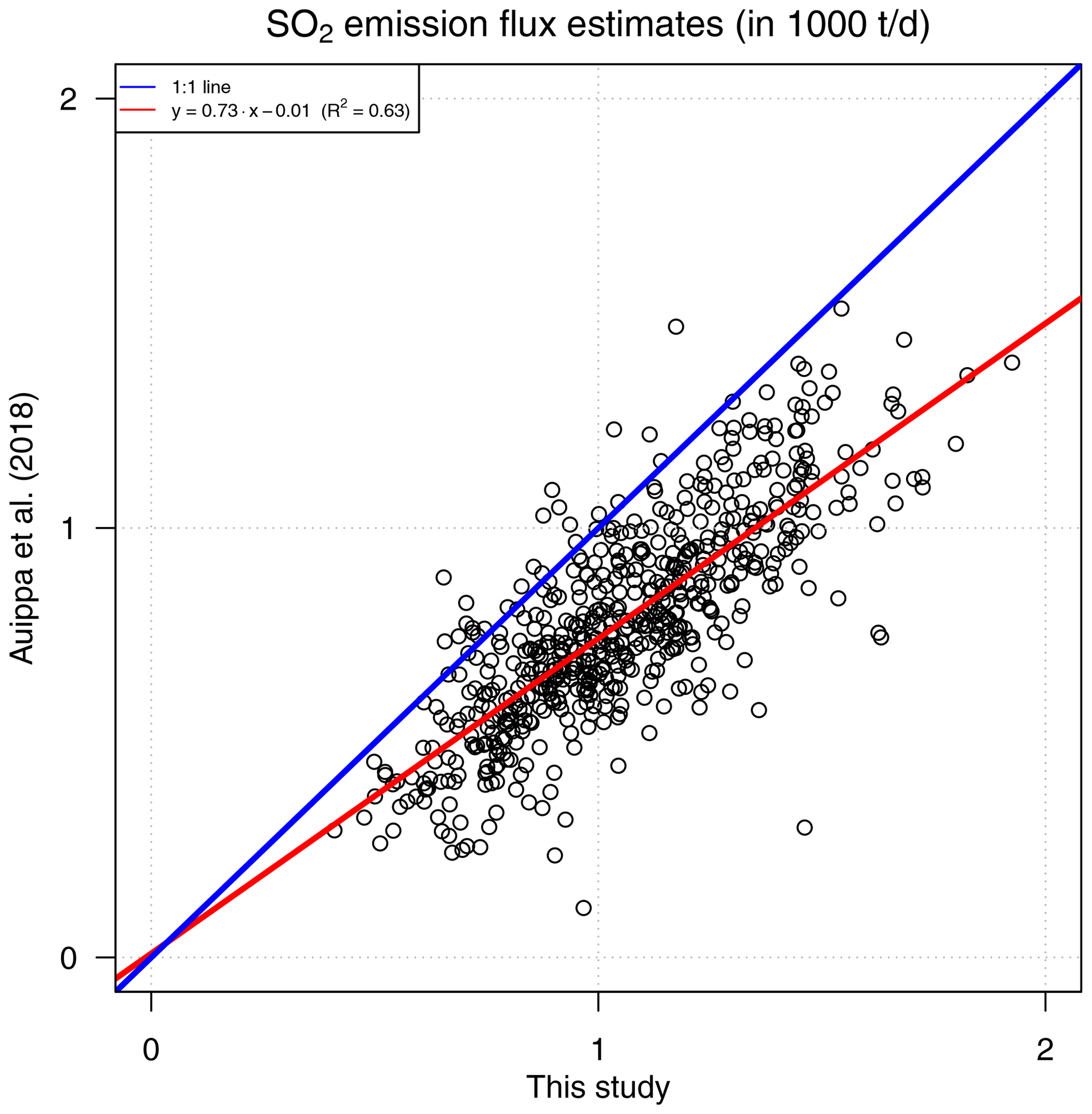
Figure 11Comparison of the SO2 emission fluxes from Caracol station reported in this study and by Aiuppa et al. (2018).
-
Aiuppa et al. (2018) used the standard NOVAC SO2 dSCD retrieval whose fit range starts as low as 310 nm. As motivated in Appendix B, we argue that they therefore may have underestimated the SO2 dSCDs at Masaya by up to a factor of 1.25 (or, to be more precise, their underestimation relative to our underestimation was up to a factor of 1.25; see Fig. B1).
-
The different estimates in the plume height explain another relative factor of (we applied on average a plume altitude of 756 m a.s.l., implying an average plume height of 374 m above Caracol station, while Aiuppa et al. (2018) applied a constant plume altitude of 635 m a.s.l., implying a plume height of 253 m above Caracol station).
-
Aiuppa et al. (2018) provided their wind data as an upload that allowed a direct comparison with our wind data. They interpolated the ERA-Interim data to the location of the volcano and used only data where the plume propagated in the proximity of Caracol station (personal communication Santiago Arellano, Chalmers University of Technology). The seasonality in their wind speed data is in good agreement with our data. The long-term ratio (from March 2014 to October 2016) between their wind speed data (interpolated to 635 m a.s.l.) and our ERA-Interim data or our operational ECMWF reanalysis data (both interpolated to 700 m a.s.l.) was 1.02 and 1.28, respectively (see also Fig. 7a). We remark that in contrast to that, actually a factor of less than 1 would be expected because of their lower retrieval altitude of 635 m a.s.l. instead of our 700 m a.s.l.
For a complete record, there are further deviations between both retrievals which manifest predominantly in the extended filtering for unstable measurement conditions in our retrieval (see Sect. 3).
We highlight nevertheless that the conditions at Masaya are rather an exception than the rule. Most NOVAC stations are usually more than 4 km away from the volcanic edifice, and their altitudes are usually more than 1 km below the altitude of the volcanic summit. In consequence, a given absolute uncertainty in the plume height of e.g. 100 m results usually in relative uncertainties in the plume height of less than 10 %. Accordingly, for other volcanoes the uncertainty in the SO2 emission fluxes may be dominated by other sources of uncertainty. Similar considerations hold for the proposed weak anti-correlation of the plume height and the wind speed.
Besides the NOVAC long-term time series, the SO2 emission fluxes of Masaya were also determined episodically by short-term (at most of several weeks) measurement campaigns. From 1976 to 2010, reported SO2 emission fluxes varied between (300±100) and (2100±900) t d−1 with all-time averages of roughly 800 t d−1 (Nadeau and Williams-Jones, 2009; Martin et al., 2010; de Moor et al., 2013). Since 2014, SO2 emission fluxes spanning between 1000 and 5000 t d−1 were reported, determined via DOAS traverse measurements (de Moor et al., 2017) or via SO2 camera measurements (Stix et al., 2018; Pering et al., 2019; Wilkes et al., 2019). Those campaign data match in general well with our observed range of SO2 emission fluxes, with the exception of most of the June 2016 data from de Moor et al. (2017) (see Fig. 10).
5.4 Critical assessment of our SO2 emission flux retrieval
This paragraph summarises the extensions implemented in our retrieval as well as a set of possible future advances which have not yet been investigated. Furthermore, the justifications for some retrieval steps introduced in Sect. 2 of this paper are motivated. The main findings are summarised in Table 6.
Table 6Applied and possible future advances in the SO2 and BrO analysis. See text for details.

-
Spectroscopic retrieval: we documented the possibility of an underestimation of the SO2 dSCDs when the SO2 DOAS fit range is not chosen appropriately (see Appendix B). For strongly degassing volcanoes, we recommend using a fit range which starts at least at 314 nm (see Table 3). Furthermore, we encourage investigating the possibility of a hybrid retrieval using an interpolation of the dSCDs retrieved from two or more fit ranges. Another source of possible errors can be a missing I0 correction of the absorption cross section of a strongly absorbing gas species. We highlight that, nevertheless, the I0 correction appears to be relevant to reduce the fit errors but is usually of negligible importance for the accuracy of the retrieved SO2 dSCD. For instance, even for SO2 dSCDs of about 4×10¹⁸ molec cm−2, the difference in the retrieved dSCDs was usually less than 1 %, but the peak-to-peak ranges of the residual structures were reduced by about 10 %–15 %. Because precision is quite relevant for the BrO retrieval but not for the SO2 retrieval, we applied the I0 correction routinely to the final data of the retrieval but not to the final data of the SO2 flux retrieval. The reason for this was the pragmatic decision to save computer run time: the effective number of spectra was more than 2 orders of magnitude lower for the retrieval than for the SO2 flux retrieval – and so was the run time required for the I0 correction. Nevertheless, we encourage the use of the I0 correction when aiming for a spectroscopically optimal retrieval.
-
Filter unstable conditions: we documented unstable measurement conditions for a significant fraction of the scans. We recommend filtering for unstable conditions, but our filters should be understood as first proposals. A logical advance would be for instance an additional check via a 2-modal Gaussian fit or applying filter thresholds which more dynamically adjust to the conditions of the investigated NOVAC station. Another filter whose potential is clearly not yet exhausted is the absolute SO2 background calibration – neither with respect to its spectroscopically optimisation nor in the use of its results. Here, we need to highlight that these filters for unstable conditions were applied only in the SO2 flux retrieval but not transferred to the retrieval. The investigation of such a filtering in the retrieval is a logical extension of the current retrieval.
-
Wind conditions: lacking measurement data for the wind conditions, the best proxies for wind data are usually weather model data. We compared the wind conditions proposed by the ECMWF ERA-Interim data ( resolution) with operational ECMWF reanalysis data (up to resolution). We documented that the ERA-Interim data proposed for Masaya were on average systematically higher wind speeds with deviations of up to 30 % for wind speeds of 20 m s−1 (or, respectively, 15 m s−1) and wind directions which were 11∘ further east–northeasterly (in contrast to easterly) than both the operational ECMWF reanalysis data and the triangulation results. We hesitated, however, to exclusively use the operational ECMWF reanalysis data due to the frequent jumps in the model set-up. As a cautious compromise, we calibrated the ERA-Interim data such that they matched the operational ECMWF reanalysis data in the long-term average and used these calibrated ERA-Interim data in all further evaluation steps (see Fig. 7a, b). We encourage, nevertheless, a comprehensive investigation of the jumps in the operational data set-up with the possible finding that exclusive use of the operational data is the best available proxy for the wind data.
-
Plume height estimate: the triangulation results documented a standard deviation of about 100 m which corresponds to a relative error of the plume height estimate of 30 %–40 % (see Fig. 7). As long as no temporally resolved information on the plume height is available, this has to be seen as a fundamental lowest limit for the uncertainty of the retrieved SO2 emission fluxes at Masaya. Furthermore, the retrieved mean plume height deviated just 100 m from the plausible best guess used by Aiuppa et al. (2018), but this deviation in the applied plume height resulted directly in a deviation by a factor of 1.5. While these numbers are extreme for Masaya and presumably less drastic for most other NOVAC volcanoes, this shows that the estimate of the plume height can be an important source of uncertainty in the SO2 emission flux retrieval. Furthermore, we observed a weak anti-correlation between the wind speed and the plume height, which is also expected because of the buoyancy of the initially hot gas plume. Ignoring this relationship could cause a spurious correlation of the SO2 emission fluxes with the wind speed (see below). We highlight that the applied triangulation algorithm is rather simple, and several advances are desired, e.g. a filter when both instruments simultaneously see different plumes (see “wings” in Fig. 6).
-
Correlation of SO2 emission flux and wind speed?: we observed a strong correlation between the original ERA-Interim wind data and the SO2 emission fluxes when these were calculated without our proposed retrieval advances (+0.84 when all wind speeds are considered, Fig. 7e). This correlation is weaker when our retrieval advances are applied (+0.71 when all wind speeds are considered) and basically vanishes for wind speeds higher than 10 m s−1 (then only +0.16, Fig. 7f). As mentioned above, this apparent correlation was most likely caused by systematics in the SO2 emission flux calculation and namely the ignorance of the variations in the plume height. Correlation checks like this should be used to validate under which measurement conditions the applied assumptions are justified. Considering Fig. 7f, we highlight that our proposed retrieval advances were able to correct this spurious correlation only for high wind speeds higher than 10 m s−1.
-
Instrument line function: we retrieved the instrument line function (ILF) from a mercury emission spectrum recorded prior to the installation of the instrument in the field (this is the standard approach for NOVAC data). The ILF varies, however, in general with temperature and due to ageing, and such variations of the ILF could be another important limitation of the accuracy of gas data from NOVAC (and presumably of most automated measurement platforms). A frequent recording of the ILF could reduce ILF-related uncertainties, but this is not always feasible at each location. Another approach would be the retrieval of the ILF directly from the recorded spectra. Such retrievals have been developed e.g. for satellite data (Sun et al., 2017) and are for example available in the QDOAS software package (http://uv-vis.aeronomie.be/software/QDOAS/, last access: 9 June 2021). However, as of today none of those retrievals has been optimised for the specifications of NOVAC instruments (i.e. rather low quality of recorded spectra and no active temperature stabilisation). The first steps in this direction have been made by Kleinbek (2020) using the HeiDOAS software package (currently under development by Udo Frieß, University of Heidelberg). Nevertheless, we highlight that both instruments enjoyed a surprisingly good long-term stability in their wavelength-to-pixel calibration, which may indicate that their ILFs were also rather stable (see variations of their wavelength-to-pixel calibration in Fig. D2). Furthermore, Dinger (2019) investigated the effect of the variations in the ILF for a NOVAC instrument installed at Nevado del Ruiz. That exemplary study concluded that for the molar ratios the ILF-related uncertainties are 1 order of magnitude smaller than the typical measurement error. While such exemplary findings cannot be adopted directly for other instruments, this has been another hint that the ILF-related effects may be in reality contribute only insignificantly to the total measurement error.
-
Network design: NOVAC has been conceptualised such that the available NOVAC stations may be distributed as a good compromise between covering most of the relevant plume propagation directions but also allowing for a retrieval of the wind direction and plume height directly via triangulation. The triangulation results presented here gave a rare opportunity to validate the use of weather model data as a proxy for the meteorological conditions at a volcano. While similar results could be retrieved also by a single NOVAC station using the optional “flux measurement mode” (Galle et al., 2010), this mode has hardly been used in the past, indicating that maintaining two rather autarkic stations is apparently more likely to happen than actively scheduling the NOVAC measurements. While there are of course financial and maintenance limitations in adding another station, we highlight that there is a significant number of NOVAC volcanoes with at least three NOVAC stations where a re-positioning of one of the stations may be beneficial in the long run. As an even further advance, McGonigle et al. (2005) demonstrated that installing three instruments in the main plume direction would also allow a direct retrieval of the wind speed.
6.1 Correlations between gas data and meteorology
We investigated the NOVAC data and ERA-Interim data for correlations. For this purpose the daily means of the SO2 dSCDs, of the BrO dSCDs, of the molar ratios, and of the SO2 emission fluxes and the noon-time ERA-Interim data were compared (Fig. 12).
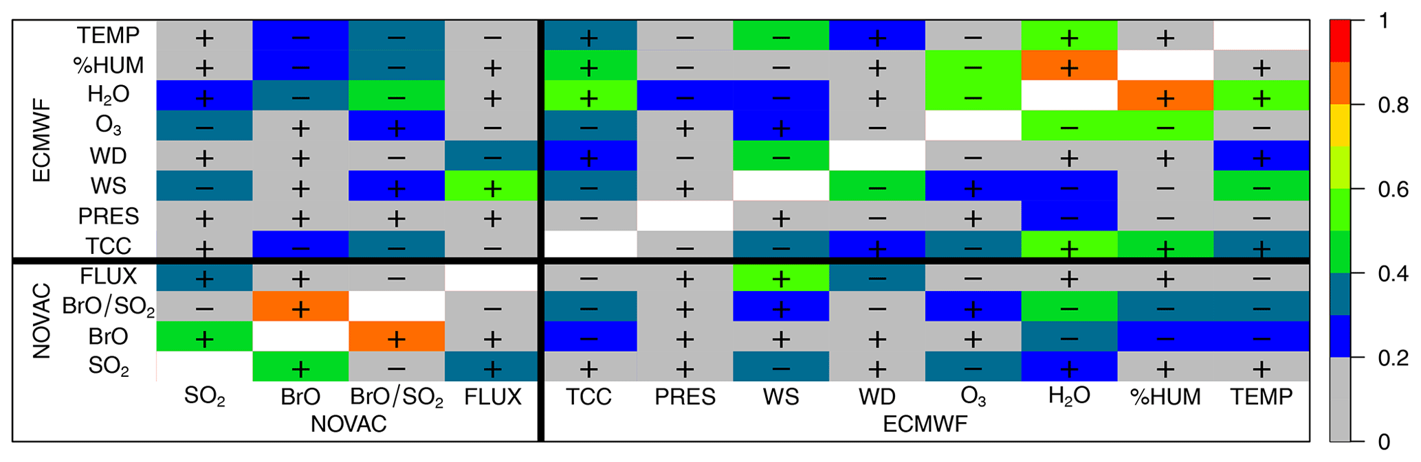
Figure 12Correlation matrix between the different NOVAC parameters and the original ECMWF ERA-Interim parameters. The colour bar indicates the absolute value of the correlation coefficient and the plus and minus signs indicate the sign of the correlation coefficient. The abbreviated parameters are, from left to right, daily means of SO2 dSCDs, BrO dSCDs, molar ratios, and SO2 emission fluxes and noon-time time series of total cloud cover, pressure, wind speed, wind direction, ozone mixing ratio, water vapour concentration, relative humidity, and ambient temperature. The auto-correlation pixels are removed for better readability.
A correlation analysis of the ERA-Interim parameters with each other indicated that (1) the barometric pressure was not correlated with any of the other parameters. (2) All remaining ERA-Interim parameters (except the wind direction) were correlated with the total cloud cover (absolute correlation coefficients between 0.36 and 0.56). This was presumably mainly a manifestation of the shared general seasonality of the weather conditions with extrema roughly in March and in October where the total cloud cover represents the seasonality apparently most clearly. (3) As expected, the three water-related parameters (water vapour concentration, relative humidity, total cloud cover) were strongly correlated and the atmospheric water vapour concentration correlated with the temperature. (4) The ozone mixing ratio was anti-correlated with the water vapour concentration (−0.55); however, this was presumably first of all the shared seasonality. (5) The wind speed and the wind direction were correlated (−0.44).
A correlation of the NOVAC parameters with each other indicated that (1) the variability in the time series originated almost exclusively from the variability in the BrO dSCDs (+0.81) and not at all from the variability in the SO2 dSCDs (−0.15). (2) The correlation between the SO2 and BrO dSCDs was far from proportional (+0.40), indicating that these two parameters were sufficiently independent of each other (i.e. the BrO data are an independent proxy for magmatic or atmospheric processes). (3) The SO2 emission fluxes were only relatively weakly correlated with the daily average of the SO2 dSCDs (+0.35). This can be explained by the two processes which presumably predominantly control the variability in the SO2 dSCDs: on the one hand, strong long-term variations in the SO2 emission flux should manifest proportionally in the long-term means of the SO2 dSCDs, but on the other hand, the variability of the SO2 dSCDs in the plume centre is also significantly controlled by the horizontal plume dispersion and thus the wind speed (see also Fig. 12). Given that the SO2 emission fluxes of Masaya have been basically constant for several years, the observed absence of such a correlation hints towards the latter reasoning.
A cross-correlation between the NOVAC data and the ERA-Interim data indicated two strong correlations: (1) a correlation between the SO2 emission fluxes and the wind speed (+0.57) and (2) an anti-correlation of the molar ratios with the water vapour concentration (−0.47). As explained above, this correlation between the SO2 emission fluxes and the wind speed was most likely predominantly an artefact because in this correlation analysis the original ERA-Interim data were used for consistency within the comparison of the meteorological data. The correlation became insignificant (+0.16) when the wind speeds are calibrated and only wind speeds higher than 10 m s−1 are considered (see Fig. 7e and f).
We highlight that the molar ratios were at most weakly correlated with the other meteorological parameters (except the water vapour concentration). In particular, the correlation coefficients with respect to the wind speed (+0.26) and the ozone mixing ratio (+0.22) were remarkably small. The correlations between the molar ratios and the three highlighted meteorological parameters are discussed in the next three paragraphs.
6.2 and atmospheric humidity
The oxidation of bromide ions (Br−) to BrO in a volcanic gas plume is an autocatalytic process; thus it is plausible that the HBr → Br− ⇌ BrO formation rate in a volcanic gas plume could be positively correlated with the Br− concentration in the aerosol phase. A slower BrO formation rate also implies a lower BrO equilibrium level because the equilibrium level of BrO/Brtotal is reached once the BrO formation rate is equalled by the rate of the BrO destruction mechanisms.
A higher humidity level could cause a smaller Br− concentration and thus a slower BrO formation rate, as supported by model simulations and experimental results (Rüdiger et al., 2018, and personal communication with Stefan Schmitt, 2019). As a remark, H+ concentration in the aerosol phase (i.e. its pH value) should be affected similarly; however, it can be expected that the H+ concentration far exceeds the Br− concentration, and thus this effect on the pH value is presumably negligible.
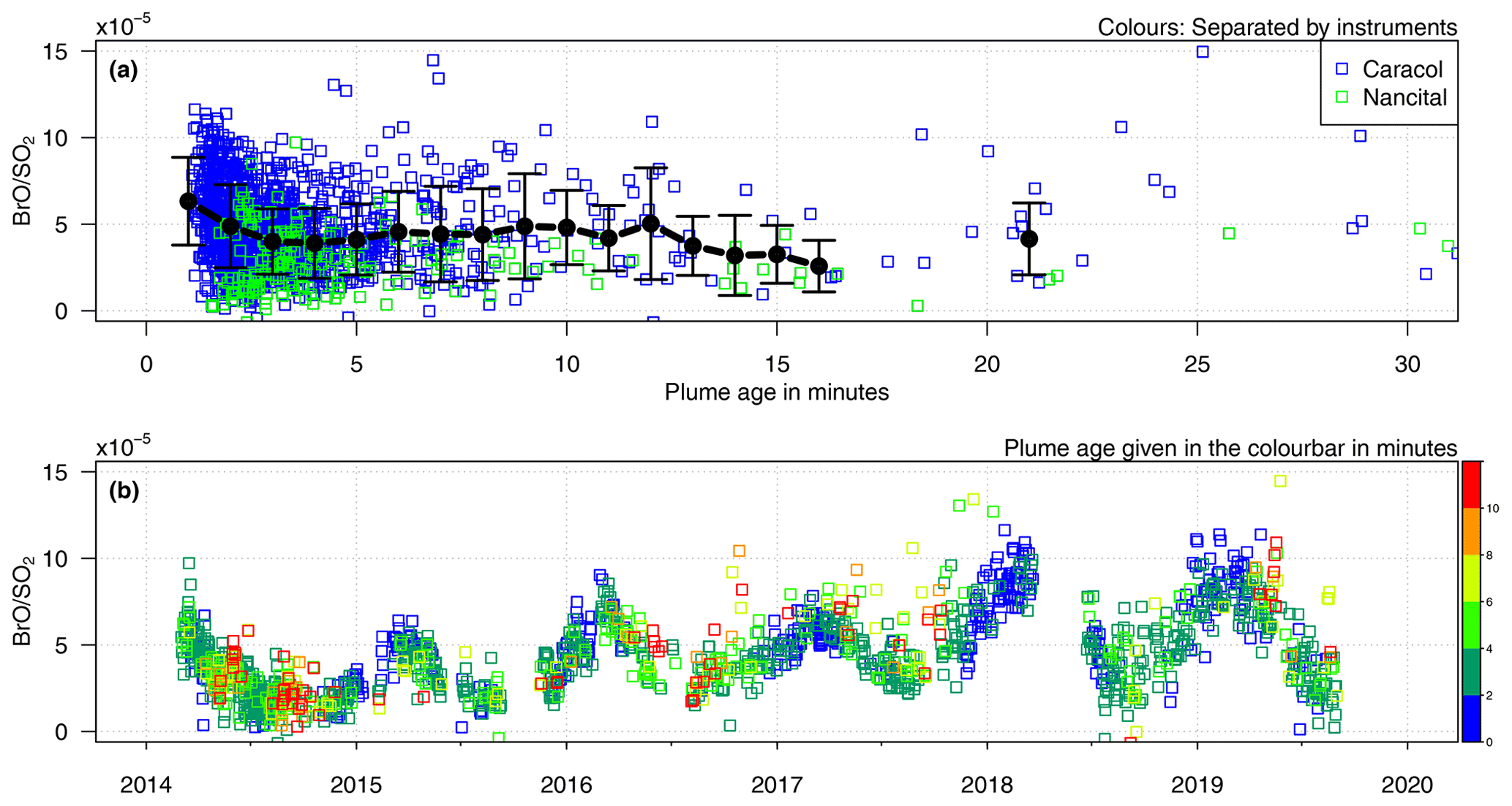
Figure 13 molar ratios in the gas plume of Masaya depending on the plume age. The wind data imply for some data that the plumes did not transact the scan planes; these data are excluded from the plot. (a) The black dots refer to the averages of the respective 1 min bins. (b) The red-coloured data span a plume age between 10 and 20 min.
The observed anti-correlation between the molar ratios and the humidity supports this hypothesis for the rather humid conditions at Masaya. Accordingly, the BrO conversion at Masaya is humidity-limited in summer and autumn when the atmospheric humidity is rather high, while this mechanism is much weaker in spring when the atmospheric humidity is in its annual minimum.
6.3 and wind conditions
The NOVAC stations at Masaya were located in close proximity to the volcanic edifice; thus they almost exclusively observed volcanic gas plumes with an atmospheric plume age between 2 and 8 min (see Fig. 13, where the calibrated wind data were used). Furthermore, almost all outliers in the time series were associated with plume ages larger than 10 min or with measurements when the plume had allegedly not transacted the scan planes at all.
The molar ratio apparently reached a maximum within the first 2 min after the release from the volcanic edifice, decreased to a slightly lower value within the third minute, and remained on this long-term equilibrium level for at least the first 20 min. We highlight that the very young plumes, whose observation indicated the early peak in the molar ratio, were observed almost exclusively in spring, when by coincidence the atmospheric humidity is also minimum and the wind speeds are maximum (Fig. 13b). This early peak may thus not necessarily imply a “fundamental overshoot” in the BrO formation but could be explained as a manifestation of higher BrO equilibrium level at times of relatively low atmospheric humidity or enhanced ozone in-mixing.
We may highlight that the lack of significant correlation between molar ratios and the plume age could be in principle also a chance result caused by two opposing wind-speed-dependent processes: on the one hand, in-mixing of ambient air (and in particular ambient ozone) would be more efficient at high wind speeds. This speeds up the chemistry but also reduces the time that elapses before the plume is measured by the NOVAC instrument. On the other hand, in-mixing is less efficient at low wind speed, but more time elapses before the ratio is measured.
As a remark for completeness: the molar ratios were not correlated with the plume altitude for March–October 2014.
6.4 and ozone mixing ratio
The bromide-to-BrO conversion requires ozone, whose destruction is catalysed by BrO. If insufficient atmospheric ozone is mixed into the volcanic plume, the BrO formation stops. The amount of ozone mixed into the plume depends on the ambient ozone background concentration and on the degree of turbulent mixing. A comparison of the data with the ERA-Interim ozone time series (Fig. 2) does not allow a detailed investigation of the chemical processes in the volcanic gas plume. Nevertheless, the ERA-Interim data allow an investigation of the Br−-to-BrO conversion in the context of the temporal variations in the general ozone availability.
On the one hand, the observed correlation coefficients between the molar ratios and the atmospheric ozone mixing ratio and the wind speeds were both rather small, indicating that the BrO conversion is not predominantly controlled by the background ozone mixing ratio or the air in-mixing rate. On the other hand, the maxima in the molar ratios coincide with the observed maxima in the wind speeds as well as in the ozone mixing ratio. Accordingly and despite the low general correlation coefficient, strong Br−-to-BrO conversion rates may be possible only for relatively large wind speeds and/or ozone background concentrations.
6.5 and SO2 emission fluxes and magmatic processes
Aiuppa et al. (2018) suggested a model, based on their data and past studies, where the (re)appearance of the lava lake on the surface was most likely caused by the enhanced magma convection supplying CO2-rich gas bubbles from minimum equivalent depths of 0.36–1.4 km. They proposed that this elevated gas bubble supply destabilised Masaya's shallow magma reservoir (<1 km depth). The model is not completely new: Rymer et al. (1998) and Williams-Jones et al. (2003) already proposed that Masaya's cyclic degassing crises are caused by convective replacement of dense, degassed magma by gas-rich vesicular magma in the shallow plumbing system (<1 km depth). Their ideas were based on results of periodic gravity surveys, and they also argued that such convective overturning is not necessarily triggered by intrusion of fresh (gas-rich) magma but may simply be initiated by degassing/crystallisation (and consequent sinking) of shallow resident magma. The data from Aiuppa et al. (2018) seem to confirm this model.
Our data are characterised by a pronounced annual cycling, but in addition we observed further changes in our gas data, which might be linked to the magma dynamics connected to the lava lake. As stated already in Aiuppa et al. (2018) and confirmed with the data presented here, no significant long-term changes in the SO2 emission fluxes were observed when the lava lake became visible at the surface. However, a step increase in the molar ratios can be noted after September 2015 (happening sometime between September and November 2015, covered by a data gap). This change in the gas composition was thus caused by variations in the volcanic bromine emissions rather than in the sulfur emissions, similar to the change in molar ratios noted by Aiuppa et al. (2018), which, respectively, was caused mainly by the variation of the CO2 emission flux. Those authors interpret these observations as evidence for supply of CO2-rich gas bubbles, sourced by enhanced magma transport and degassing at a depth > (0.36–1.4) km. Following their interpretation and assuming that BrO is somehow an indicator of bromine emissions, that would mean that either also bromine is degassing below that depth or that there is another process which leads to an enhanced transformation of HBr into BrO.
By ignoring the latter possibility, the increasing molar ratios would thus indicate that bromine degasses together with or is enhanced/driven by CO2 degassing. Unfortunately, there are to our knowledge no studies (apart from conceptual models) to prove or disprove the counter-intuitive early degassing of halogens, specifically bromine. However, Bobrowski et al. (2017) also described a similar behaviour between and in connection with a lava lake level change.
Aiuppa et al. (2018) further observed an increase in the SO2 degassing after the appearance of the lava lake at the surface, which is a further argument for their hypothesis for a faster shallow magma convection. Our data confirm an enhancement of the mean SO2 emission fluxes by 30 % for the period from December 2015 to February 2016 when compared with the previous and subsequent degassing behaviour. The described observation of Aiuppa et al. (2018) ends with March 2017. The decrease in the lava lake activity in mid-2018 is therefore not described by those authors. We here report a significant decrease in the SO2 emission fluxes after June 2018 (happening sometime between March and June 2018, covered by a data gap), while the molar ratios hardly changed. This decrease in the SO2 emission fluxes in time in connection with the decrease in the lava lake activity is consistent with the interpretation that the convection of the magma inside the conduit below the upper reservoir slowed down again after 2018, and an important further indicator to sustain this hypothesis could be additional molar ratios. Unfortunately no molar ratios were available to the authors at the time of writing of the paper.
An unchanged ratio and a lower SO2 emission flux would lead to lower bromine emission as well, if we assume a correlation of bromine emissions and amount of BrO. We might further speculate that the bromine emission and carbon emission are characterised again by a similar pattern, which would mean that we also see a decrease in the CO2 emission flux.
This study contributes to three independent fields of research: (1) a comprehensive discussion of a reliable retrieval of SO2 emission fluxes from ground-based remote sensing data, (2) a data set for the bromine chemistry in volcanic gas plumes with extraordinary temporal coverage and resolution, and (3) an investigation of the molar ratio as a proxy for magmatic processes.
7.1 SO2 emission flux retrieval
An important conclusion of our study is the reminder that calculating reliable SO2 emission fluxes requires a careful investigation of the local conditions. This holds true not only for their accuracy, but also for the patterns in the data.
We reported suggestions for the retrieval of SO2 emission fluxes from ground-based remote sensing data and retrieved SO2 emission fluxes, which are on average a factor of 1.4 larger than those retrieved by Aiuppa et al. (2018) from the same spectroscopic data. This factor is an accumulation of three major differences between the two retrieval approaches: the SO2 fit range, the wind speed estimate, and the plume height estimate. (1) The different choices of the SO2 fit ranges (our range starts at 314 nm, theirs starts at 310 nm) causes a relative factor of 1.25, indicating their systematic underestimation of the rather strong SO2 SCDs in Masaya's gas plume. (2) Both studies estimated the wind speeds based on ERA-Interim data, but we calibrated those wind speeds to the local conditions by using the higher resolved operational ECMWF reanalysis data. In consequence, our estimates for the wind speeds are on average a factor of 0.8 smaller than theirs. (3) Aiuppa et al. (2018) assumed a plume height fixed at Masaya's summit altitude, while we used a dynamic estimate of the plume height based on our triangulation results and the observed weak dependency on the wind speed. In consequence, our estimates for the plume height were on average a factor of 1.5 larger than theirs.
When it comes to spurious patterns, we observed a strong correlation between the SO2 emission fluxes and the wind speeds when several of our retrieval extensions are not applied (correlation coefficient of +0.84 when all wind speeds are considered and of +0.56 for wind speeds higher than 10 m s−1). We showed that no such correlation is expected and that it is most likely an artefact, e.g. due to the assumed fixed plume height. In consequence, the SO2 emission fluxes would then falsely inherit patterns from the variability of the wind speeds, and thus conclusions drawn from the variability of the SO2 emission fluxes would be only of limited reliability. The correlation was significantly reduced (+0.71) after retrieval extensions were applied and in particular basically vanished for wind speeds higher than 10 m s−` (+0.16). Another conclusion is thus that low wind speeds can result in rather unreliable results (at least at Masaya).
We encourage future publications on SO2 emission fluxes to state detailed information on the used SO2 emission retrieval algorithm. The investigation strategy presented in this study may provide a framework for that task. We nevertheless highlight the large set of further possible advances which can still be applied and highlight that the choice and setting of the filters may vary significantly for different volcanoes.
7.2 Atmospheric bromine chemistry
We observed an annual cyclicity in the time series. This annual cyclicity was most likely a manifestation of the meteorological seasonality. In particular, an anti-correlation (coefficient of −0.47) was observed between the molar ratios and the atmospheric water vapour concentration. In contrast to that, no clear correlation was observed between the molar ratios and the atmospheric ozone mixing ratio (coefficient of +0.21) or the wind speed (coefficient of +0.25). A comparison of the molar ratio and the atmospheric age of the volcanic plume suggested that the reached in the long-term average maximum values within the first 2 min after the release from the volcanic edifice, dropped to a slightly lower level within the third minute, and remained at this level for at least the next 20 min. The enhancement prior to the third minute may be real but could also be explained by an observational bias. We conclude that the BrO formation rate at Masaya may be partly controlled by the rather high ambient humidity, with higher humidity leading to dilution of the bromide concentration in the aerosol phase and thus a lower BrO conversion rate.
7.3 Volcanological findings
We observed a complementary sensitivity of the SO2 emission fluxes and the molar ratios to magmatic processes. The long-term trend of the SO2 emission fluxes was hardly affected by the initial lava lake appearance but dropped in mid 2018, when the lava lake activity ceased, to significantly lower SO2 emission fluxes. In contrast to that, the molar ratios doubled due to the lava lake appearance but showed only a weak response to the reduced lava lake activity since mid 2018. Accordingly, the combination of SO2 emission fluxes and molar ratios – the latter one showing a similar behaviour to the molar ratios for the period both data sets are available – might give new possibilities for monitoring.
When corrected for the annual cyclicity, we observed an approximately linearly increasing trend in the molar ratios during the period for high lava lake activity (November 2015 until March 2018) and an approximately linearly decreasing trend in the molar ratios since May 2018. The isolated interpretation of these observations did not provide clear information on e.g. the degassing order of sulfur and bromine of the juvenile magma at Masaya. However, the provided data may help to double-check and enhance models on the magmatic processes at Masaya.
The ground-based data from Managua airport are recorded at an altitude of 59 m a.s.l., and thus their quantitative values are expected to differ from the meteorological data modelled for 700 m a.s.l. Nevertheless, the ground base data agree with the ERA-Interim data in the general patterns and relative variations, with variations in the ambient temperature between 302 and 307 K, variations in the relative humidity between 40 % and 70 %, variations in the wind speeds between 2 and 8 m s−1, and a mean wind direction of (86±31)∘ (Fig. A1). The wind directions differ significantly with (102±29)∘ when considering all times of the day.

Figure A1Meteorological conditions measured by a ground-based station at Managua airport (15 km north of Masaya volcano). The data were provided by Iowa State University (https://mesonet.agron.iastate.edu, last access: 9 June 2021). Grey lines: hourly data. Blue lines: sliding average over the hourly data (±2-week window). Black dots: noon-time (18:00 UTC) data. Red lines: same sliding average but over the around-noon data.
The choice of the wavelength range (and in particular its lower limit) used in the SO2 DOAS fit can cause major deviations in the spectroscopic results. The standard NOVAC evaluation routine uses 310 nm for the lower limit because this value is optimal for detecting low SO2 dSCDs of several 1017 molec cm−2 (which is the case for volcanoes with a low to moderate degassing strength or considerable distances of the DOAS instrument to the emission source). As a drawback, such a short wavelength for the lower limit makes the SO2 DOAS fit susceptible to saturation effects and spectrometer stray light, resulting in an underestimation of SO2 dSCDs larger than 1×10¹⁸ molec cm−2 (see Fig. B1a and e.g. Bobrowski et al., 2010; Fickel and Delgado Granados, 2017). In contrast to that, our choice of 314.9–326.8 nm can be considered to be hardly affected by saturation effects up to SO2 SCDs of 1×10¹⁸ molec cm−2 (3 % underestimation; see Fig. B1b) and still of acceptable accuracy at SO2 SCDs of 3×10¹⁸ molec cm−2 (9 % underestimation). We observed at Masaya, nevertheless, a significant amount of data with SO2 SCDs above 3×10¹⁸ molec cm−2 which were underestimated also by our retrieval (Figs. B1b and 8). A separated retrieval of those data with an alternative fit range starting e.g. at 319 nm would in general result in more accurate estimates for these particularly large SO2 SCDs. Fickel and Delgado Granados (2017) proposed such an approach for Popocatépetl using even three wavelength ranges at 310–322, 314.7–326.7, and 322–334 nm. The risk of such a compound retrieval would be, however, artificial jumps along the chosen thresholds. We therefore hesitated to use such an approach but encourage further investigations, e.g. whether an interpolation between the results retrieved by several fit ranges could avoid this risk while enhancing the accuracy of large SO2 SCDs (see e.g. Theys et al., 2017; Elias et al., 2018, for the implementation of such an approach in satellite and ground-based observations, respectively).
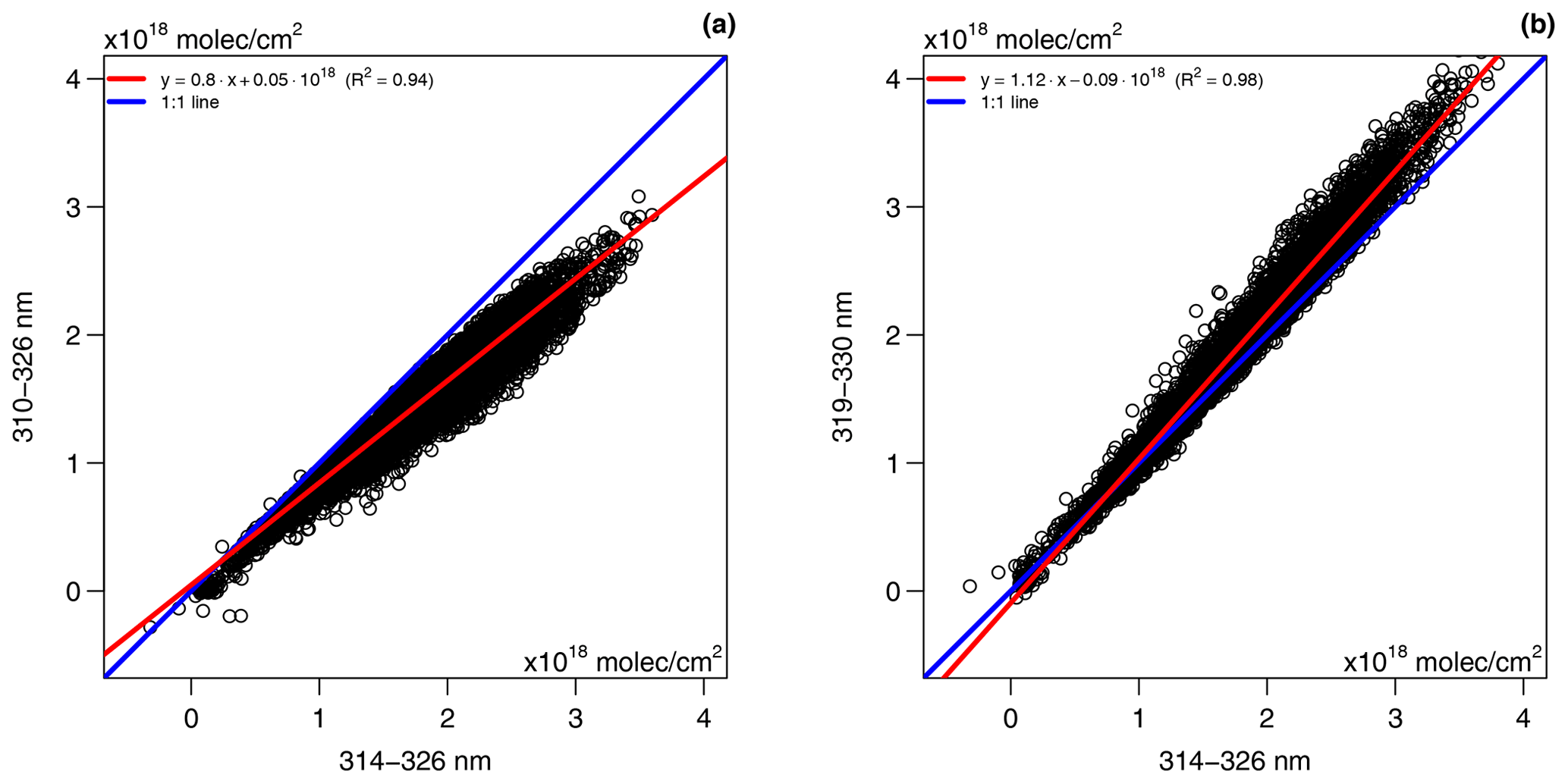
Figure B1SO2 dSCDs retrieved in the chosen wavelength range compared with those retrieved in other wavelength ranges, as retrieved for Caracol station from 2014 to 2020. For statistical interpretation of the 314–326 nm data, 9 % of the SO2 dSCDs were lower than 1×10¹⁸ molec cm−2, 63 % were between 1 and 2×10¹⁸ molec cm−2, 26 % were between 2 and 3×10¹⁸ molec cm−2, and 2 % were larger than 3×10¹⁸ molec cm−2.
We checked for an SO2 contamination of the background by applying the absolute calibration algorithm described by Lübcke et al. (2016). This algorithm performs SO2 DOAS fits where the recorded added-reference spectrum is used as the measurement spectrum and the solar atlas provided by Chance and Kurucz (2010) – convoluted with the instrument line function – is used as the reference spectrum. Such a fit results in large residual spectroscopic structures because the solar atlas does not contain information on the instrument characteristics. These characteristics can, nevertheless, be determined from the fit residual structures via a principal component analysis applied to a time series of the residual structures. Hereby, it is important that the principal components do not contain structures caused by an interference with the major absorbers in the investigated wavelength range. Accordingly, we used only those residual structures for the principal component analysis (1) where the retrieved SO2 SCD was smaller than 2 times the (individual) SO2 fit error, (2) where the solar elevation angle was >30∘ to avoid large tropospheric ozone columns, and (3) where the SO2 fit had a fit quality of χ2<0.1 to avoid potentially problematic spectra. We retrieved a unique fixed first principal component for the total 6-year time series and added it as a pseudo-absorber to the DOAS fit. This second iteration of the DOAS retrieval gave the absolute SO2 SCD of the added-reference spectrum (see histograms of these results in Fig. 7c). We highlight that the second principal component for the total 6-year time series explains only 1 % of the residual structures, and thus adding this component to the fit scenario would not have improved the spectroscopic retrieval.
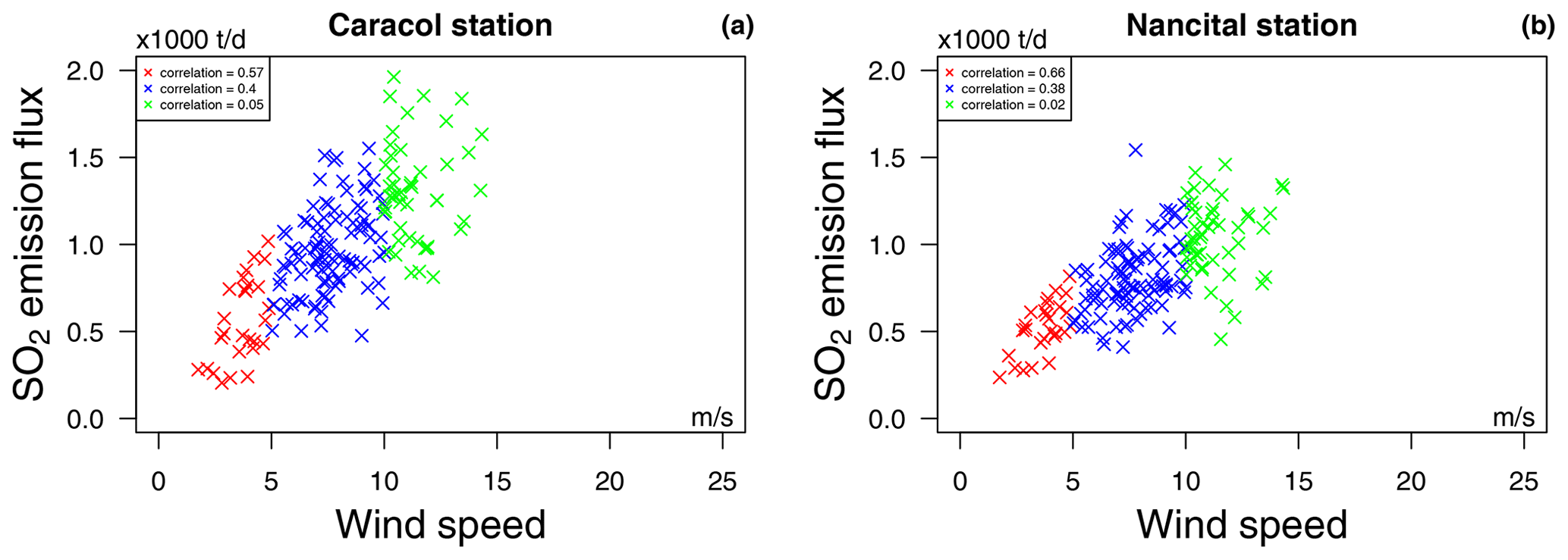
Figure D1Correlation between the retrieved SO2 emission fluxes and the wind speed for March to October 2014 and when the triangulation results are directly used. The plots compare daily SO2 means and the means of the calibrated wind speed at the respective measurement times. The fluxes were calculated based on the triangulated plume height and plume propagation direction and based on the calibrated wind speeds.
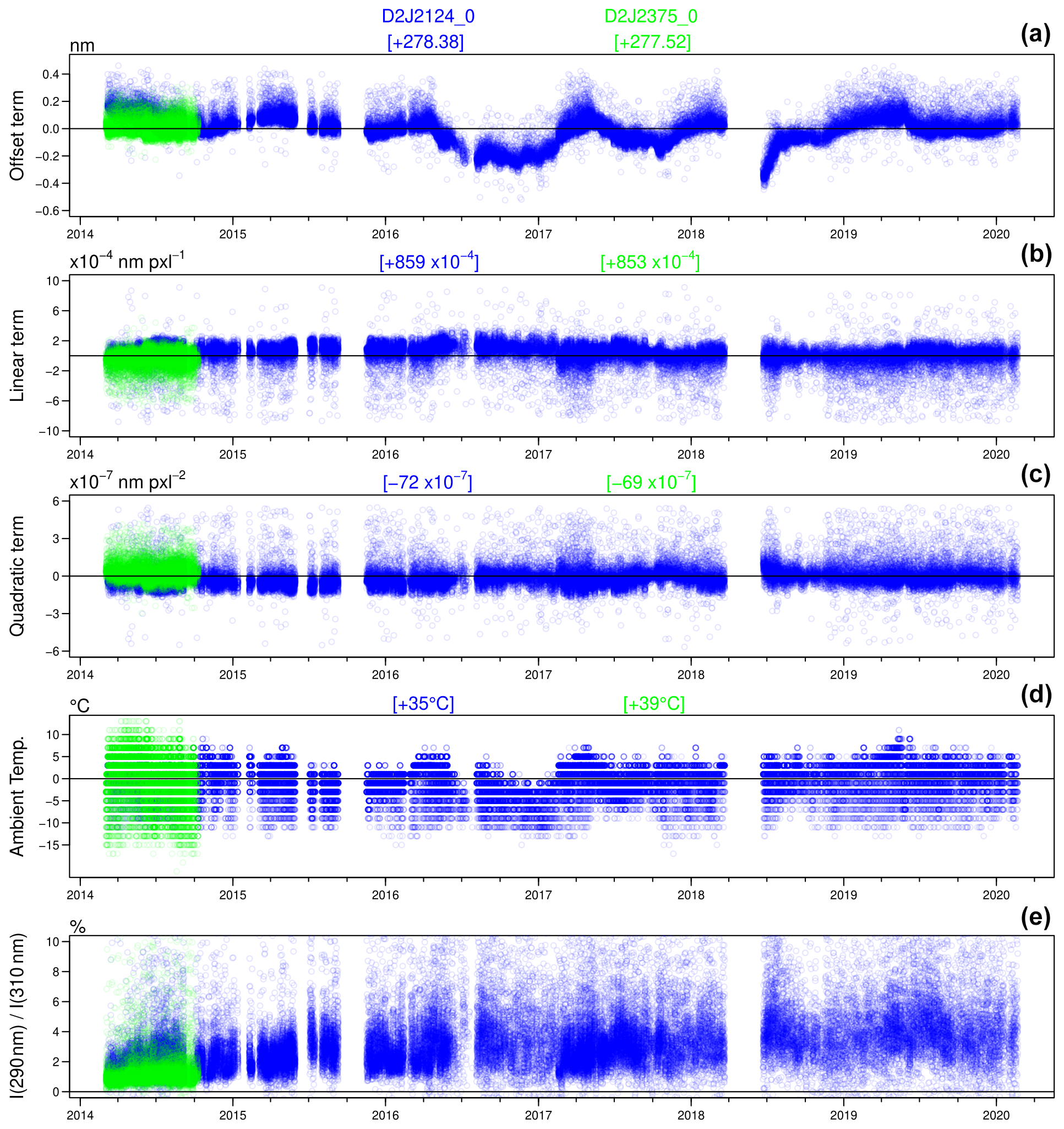
Figure D2Variation of the instruments' wavelength-to-pixel calibration and stray light and the ambient temperature. For each parameter, the total values are given by the rough estimate for the mean value (given for each instrument in blue and green above the particular panel) and the variation shown in the plots. The zero lines are chosen arbitrarily and should not be confused with mean values. (a–c) All spectra were calibrated by matching their Fraunhofer lines with the Fraunhofer lines of a solar atlas, and wavelength calibration was given by a calibration polynomial of second order (see e.g. Dinger, 2019, for details). The three panels give for each scan the three coefficients of the wavelength calibration polynomial. The variability is already as displayed rather low but is actually much lower (most of the indicated scatter is predominantly caused by the first scans in the morning when the temperature is significantly lower than for the rest of the day). (d) Variation of the ambient temperature. (e) Ratio of the intensity at around 290 and 310 nm (each time average over 10 channels) as a proxy for the magnitude and variation of the stray light.
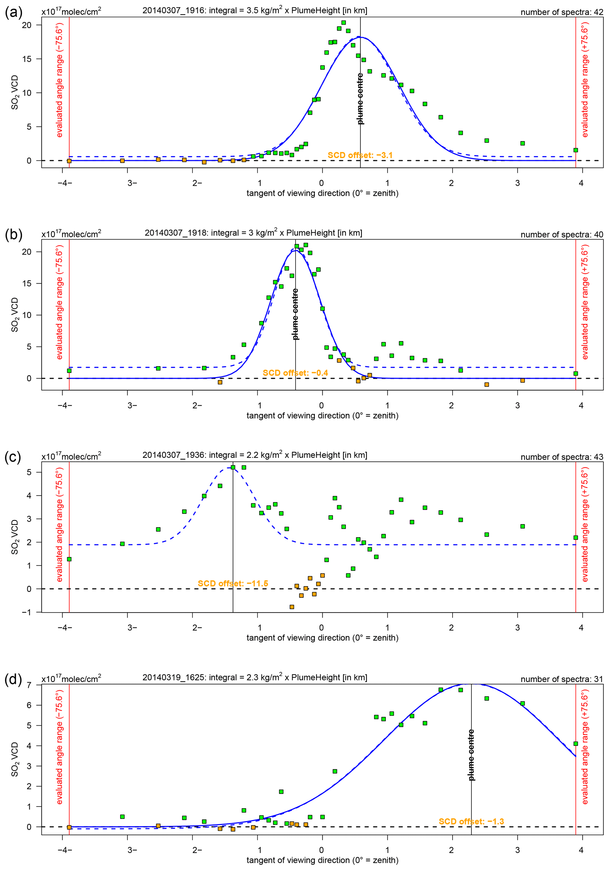
Figure D3SO2 distribution retrieved (a) from the scan starting at 7 March 2014 19:16 UTC recorded at Nancital station and (b–d) from the scans starting at 7 March 2014 19:18 UTC, 7 March 2014 19:36 UTC, and 19 March 2014 16:25 UTC recorded at Caracol station.
Please refer to the author list for access to the code.
The time series of the SO2 SCDs, of the BrO SCDs, of the SO2 emission fluxes, of the molar ratios, and of several filter parameters can be access on https://doi.org/10.11588/data/IX51KS (Dinger et al., 2021). Raw spectral data used to obtain the results presented in this study have been acquired within the NOVAC collaboration. Access to these data is permitted with consent of the respective volcanological observatories that own the source instruments, according to their internal policies for data administration. Access to the presented meteorological data is possible with an ECMWF licence.
Data provision: MI and EE provided the raw spectrosopic data. FD and TK retrieved the spectroscopic results. SD and FD provided and processed the weather data. Data analysis: FD performed the statistical data analysis. FD, TW, UP, and NB assessed the retrieval method of SO2 emission fluxes and molar ratios. Discussion: FD, TW, UP, NB, and SD discussed the implications of the data for the atmospheric bromine chemistry. NB, FD, MI, and EE discussed the implications of the data for volcanology. FD wrote the manuscript. NB, UP, TW, and SD contributed to text editing.
The authors declare that they have no conflict of interest.
We express our thanks to Santiago Arellano for critically reading our manuscript and for helpful discussions. Florian Dinger wants to thank Stefan Schmitt (IUP Heidelberg) for fruitful discussions on the bromine chemistry in volcanic gas plumes. We would like to thank Tom Pering and Christopher Kern for their comments on the paper.
This work has been supported by the Deutsche Forschungsgemeinschaft within project DFG PL193/14-1.
The article processing charges for this open-access publication were covered by the Max Planck Society.
This paper was edited by Markus Ammann and reviewed by Christoph Kern, Tom D. Pering and one anonymous referee.
Aiuppa, A.: Degassing of halogens from basaltic volcanism: Insights from volcanic gas observations, Chem. Geol., 263, 99–109, https://doi.org/10.1016/j.chemgeo.2008.08.022, 2009. a
Aiuppa, A., Federico, C., Franco, A., Giudice, G., Gurrieri, S., Inguaggiato, S., Liuzzo, M., McGonigle, A. J. S., and Valenza, M.: Emission of bromine and iodine from Mount Etna volcano, Geochem. Geophy. Geosy., 6, Q08008, https://doi.org/10.1029/2005GC000965, 2005. a
Aiuppa, A., Federico, C., Giudice, G., Gurrieri, S., Liuzzo, M., Shinohara, H., Favara, R., and Valenza, M.: Rates of carbon dioxide plume degassing from Mount Etna volcano, J. Geophys. Res.-Solid, 111, B09207, https://doi.org/10.1029/2006JB004307, 2006. a
Aiuppa, A., Robidoux, P., Tamburello, G., Conde, V., Galle, B., Avard, G., Bagnato, E., De Moor, J. M., Martínez, M., and Muñóz, A.: Gas measurements from the Costa Rica–Nicaragua volcanic segment suggest possible along-arc variations in volcanic gas chemistry, Earth Planet. Sc. Lett., 407, 134–147, 2014. a
Aiuppa, A., de Moor, J. M., Arellano, S., Coppola, D., Francofonte, V., Galle, B., Giudice, G., Liuzzo, M., Mendoza, E., Saballos, A., Tamburello, G., Battaglia, A., Bitetto, M., Gurrieri, S., Laiolo, M., Mastrolia, A., and Moretti, R.: Tracking Formation of a Lava Lake From Ground and Space: Masaya Volcano (Nicaragua), 2014–2017, Geochem. Geophy. Geosy., 19, 496–515, https://doi.org/10.1002/2017GC007227, 2018. a, b, c, d, e, f, g, h, i, j, k, l, m, n, o, p, q
Allard, P., Burton, M., and Muré, F.: Spectroscopic evidence for a lava fountain driven by previously accumulated magmatic gas, Nature, 433, 407–410, https://doi.org/10.1038/nature03246, 2005. a
Baxter, P., Stoiber, R., and Williams, S.: Volcanic Gases And Health: Masaya Volcano, Nicaragua, Lancet, 320, 150–151, 1982. a
Bobrowski, N. and Giuffrida, G.: Bromine monoxide/sulphur dioxide ratios in relation to volcanological observations at Mt. Etna 2006–2009, Solid Earth, 3, 433–445, https://doi.org/10.5194/se-3-433-2012, 2012. a, b, c
Bobrowski, N. and Platt, U.: Quantification of volcanic reactive halogen emissions, in: chap. 24, Cambridge University Press, Cambridge, 2015. a, b
Bobrowski, N., Hönninger, G., Galle, B., and Platt, U.: Detection of bromine monoxide in a volcanic plume, Nature, 423, 273–276, https://doi.org/10.1038/nature01625, 2003. a
Bobrowski, N., von Glasow, R., Aiuppa, A., Inguaggiato, S., Louban, I., Ibrahim, O. W., and Platt, U.: Reactive halogen chemistry in volcanic plumes, J. Geophys. Res.-Atmos., 112, d06311, https://doi.org/10.1029/2006JD007206, 2007. a, b
Bobrowski, N., Kern, C., Platt, U., Hörmann, C., and Wagner, T.: Novel SO2 spectral evaluation scheme using the 360–390 nm wavelength range, Atmos. Meas. Tech., 3, 879–891, https://doi.org/10.5194/amt-3-879-2010, 2010. a
Bobrowski, N., Giuffrida, G. B., Yalire, M., Lübcke, P., Arellano, S., Balagizi, C., Calabrese, S., Galle, B., and Tedesco, D.: Multi-component gas emission measurements of the active lava lake of Nyiragongo, DR Congo, J. Afr. Earth Sci., 134, 856–865, 2017. a
Burrows, J. P., Richter, A., Dehn, A., Deters, B., Himmelmann, S., Voigt, S., and Orphal, J.: Atmospheric remote-sensing reference data from GOME. 2. Temperature dependent absorption cross sections of O3 in the 231–794 nm range, J. Quant. Spectrosc. Ra., 61, 509–517, https://doi.org/10.1016/S0022-4073(98)00037-5, 1999. a
Burton, M., Mader, H., and Polacci, M.: The role of gas percolation in quiescent degassing of persistently active basaltic volcanoes, Earth Planet. Sc. Lett., 264, 46–60, https://doi.org/10.1016/j.epsl.2007.08.028, 2007. a
Butz, A., Dinger, A. S., Bobrowski, N., Kostinek, J., Fieber, L., Fischerkeller, C., Giuffrida, G. B., Hase, F., Klappenbach, F., Kuhn, J., Lübcke, P., Tirpitz, L., and Tu, Q.: Remote sensing of volcanic CO2, HF, HCl, SO2, and BrO in the downwind plume of Mt. Etna, Atmos. Meas. Tech., 10, 1–14, https://doi.org/10.5194/amt-10-1-2017, 2017. a
Carn, S. A., Fioletov, V. E., McLinden, C. A., Li, C., and Krotkov, N. A.: A decade of global volcanic SO2 emissions measured from space, Scient. Rep., 7, 44095, https://doi.org/10.1038/srep44095, 2017. a
Carroll, M. R. and Holloway, J. R. (Eds.): Volatiles in Magma, De Gruyter, Mineralogical Society Of America, BookCrafters, Inc., Fredericksburg, Virginia, 1994. a
Chance, K. and Kurucz, R.: An improved high-resolution solar reference spectrum for earth's atmosphere measurements in the ultraviolet, visible, and near infrared, J. Quant. Spectrosc. Ra., 111, 1289–1295, https://doi.org/10.1016/j.jqsrt.2010.01.036, 2010. a, b
Delmelle, P., Stix, J., Baxter, P., Garcia-Alvarez, J., and Barquero, J.: Atmospheric dispersion, environmental effects and potential health hazard associated with the low-altitude gas plume of Masaya volcano, Nicaragua, Bull. Volcanol., 64, 423–434, https://doi.org/10.1007/s00445-002-0221-6, 2002. a
de Moor, J. M., Fischer, T. P., Sharp, Z. D., King, P. L., Wilke, M., Botcharnikov, R. E., Cottrell, E., Zelenski, M., Marty, B., Klimm, K., Rivard, C., Ayalew, D., Ramirez, C., and Kelley, K. A.: Sulfur degassing at Erta Ale (Ethiopia) and Masaya (Nicaragua) volcanoes: Implications for degassing processes and oxygen fugacities of basaltic systems, Geochem. Geophy. Geosy., 14, 4076–4108, https://doi.org/10.1002/ggge.20255, 2013. a
de Moor, J. M., Kern, C., Avard, G., Muller, C., Aiuppa, A., Saballos, A., Ibarra, M., LaFemina, P., Protti, M., and Fischer, T. P.: A New Sulfur and Carbon Degassing Inventory for the Southern Central American Volcanic Arc: The Importance of Accurate Time-Series Data Sets and Possible Tectonic Processes Responsible for Temporal Variations in Arc-Scale Volatile Emissions, Geochem. Geophy. Geosy., 18, 4437–4468, https://doi.org/10.1002/2017GC007141, 2017. a, b
de Oviedo, G. F.: Historia general y natural de las Indias, edited by: Amador de los Ríos, J., Real Academia de la Historia, Spain, available at: https://archive.org/details/historiageneraly01fern/mode/2up (last access: 9 June 2021), 1855. a
Dinger, F.: On long-term variations in the BrO/SO2 molar ratios in volcanic gas plumes, PhD thesis, Johannes Gutenberg University of Mainz, Mainz, Germany, 2019. a, b, c
Dinger, F., Bobrowski, N., Warnach, S., Bredemeyer, S., Hidalgo, S., Arellano, S., Galle, B., Platt, U., and Wagner, T.: Periodicity in the molar ratios in the volcanic gas plume of Cotopaxi and its correlation with the Earth tides during the eruption in 2015, Solid Earth, 9, 247–266, https://doi.org/10.5194/se-9-247-2018, 2018. a
Dinger, F., Kleinbek, T., Dörner, S., Bobrowski, N., Platt, U., Wagner, T., Ibarra, M., and Espinoza, E.: SO2 and BrO emissions of Masaya volcano from 2014 to 2020 [Research Data], heiDATA, V1, https://doi.org/10.11588/data/IX51KS, 2021. a
Donovan, A., Tsanev, V., Oppenheimer, C., and Edmonds, M.: Reactive halogens (BrO and OClO) detected in the plume of Soufrière Hills Volcano during an eruption hiatus, Geochem. Geophy. Geosy., 15, 3346–3363, https://doi.org/10.1002/2014GC005419, 2014. a
Edmonds, M., Pyle, D., and Oppenheimer, C.: A model for degassing at the Soufrière Hills Volcano, Montserrat, West Indies, based on geochemical data, Earth Planet. Sc. Lett., 186, 159–173, https://doi.org/10.1016/S0012-821X(01)00242-4, 2001. a
Edmonds, M., Herd, R. A., Galle, B., and Oppenheimer, C. M.: Automated, high time-resolution measurements of SO2 flux at Soufrière Hills Volcano, Montserrat, Bull. Volcanol., 65, 578–586, https://doi.org/10.1007/s00445-003-0286-x, 2003. a
Elias, T., Kern, C., Horton, K. A., Sutton, A. J., and Garbeil, H.: Measuring SO2 Emission Rates at Kīlauea Volcano, Hawaii, Using an Array of Upward-Looking UV Spectrometers, 2014–2017, Front. Earth Sci., 6, 214, https://doi.org/10.3389/feart.2018.00214, 2018. a
Esse, B., Burton, M., Varnam, M., Kazahaya, R., and Salerno, G.: iFit: A simple method for measuring volcanic SO2 without a measured Fraunhofer reference spectrum, J. Volcanol. Geoth. Res., 402, 107000, https://doi.org/10.1016/j.jvolgeores.2020.107000, 2020. a
Fickel, M. and Delgado Granados, H.: On the use of different spectral windows in DOAS evaluations: Effects on the estimation of SO2 emission rate and mixing ratios during strong emission of Popocatépetl volcano, Chem. Geol., 462, 67–73, 2017. a, b
Fischer, T. P., Arellano, S., Carn, S., Aiuppa, A., Galle, B., Allard, P., Lopez, T., Shinohara, H., Kelly, P., Werner, C., Cardellini, C., and Chiodini, G.: The emissions of CO2 and other volatiles from the world's subaerial volcanoes, Scient. Rep., 9, 18716, https://doi.org/10.1038/s41598-019-54682-1, 2019. a
Fleischmann, O. C., Hartmann, M., Burrows, J. P., and Orphal, J.: New ultraviolet absorption cross-sections of BrO at atmospheric temperatures measured by time-windowing Fourier transform spectroscopy, J. Photochem. Photobiol. A, 168, 117–132, https://doi.org/10.1016/j.jphotochem.2004.03.026, 2004. a
Galle, B., Oppenheimer, C., Geyer, A., McGonigle, A. J., Edmonds, M., and Horrocks, L.: A miniaturised ultraviolet spectrometer for remote sensing of SO2 fluxes: a new tool for volcano surveillance, J. Volcanol. Geoth. Res., 119, 241–254, https://doi.org/10.1016/S0377-0273(02)00356-6, 2003. a
Galle, B., Johansson, M., Rivera, C., Zhang, Y., Kihlman, M., Kern, C., Lehmann, T., Platt, U., Arellano, S., and Hidalgo, S.: Network for Observation of Volcanic and Atmospheric Change (NOVAC) – A global network for volcanic gas monitoring: Network layout and instrument description, J. Geophys. Res.-Atmos., 115, d05304, https://doi.org/10.1029/2009JD011823, 2010. a, b, c, d
Giggenbach, W. F.: Chemical Composition of Volcanic Gases, Springer, Berlin, Heidelberg, 221–256, https://doi.org/10.1007/978-3-642-80087-0_7, 1996. a
Gliß, J., Bobrowski, N., Vogel, L., Pöhler, D., and Platt, U.: OClO and BrO observations in the volcanic plume of Mt. Etna – implications on the chemistry of chlorine and bromine species in volcanic plumes, Atmos. Chem. Phys., 15, 5659–5681, https://doi.org/10.5194/acp-15-5659-2015, 2015. a, b, c
Global Volcanism Program: Report on Masaya (Nicaragua), in: Bulletin of the Global Volcanism Network, edited by: Krippner, J. B. and Venzke, E., Smithsonian Institution, 2018. a, b, c
Grainer, J. F. and Ring, J.: Anomalous Fraunhofer Line Profiles, Nature, 193, 762–762, https://doi.org/10.1038/193762a0, 1962. a
Gutmann, A., Bobrowski, N., Roberts, T. J., Rüdiger, J., and Hoffmann, T.: Advances in Bromine Speciation in Volcanic Plumes, Front. Earth Sci., 6, 213, https://doi.org/10.3389/feart.2018.00213, 2018. a
Hermans, C., Vandaele, A. C., Fally, S., Carleer, M., Colin, R., Coquart, B., Jenouvrier, A., and Merienne, M.-F.: Absorption Cross-section of the Collision-Induced Bands of Oxygen from the UV to the NIR, Springer Netherlands, Dordrecht, 193–202, https://doi.org/10.1007/978-94-010-0025-3_16, 2003. a
INETER: Boletín mensual Sismos y Volcanes de Nicaragua, Noviembre 2015, Tech. rep., available at: https://webserver2.ineter.gob.ni/boletin/2015/11/boletin-1511.pdf (last access: 9 June 2021), 2015a. a, b
INETER: Boletín mensual Sismos y Volcanes de Nicaragua, Diciembre 2015, Tech. rep., available at: https://webserver2.ineter.gob.ni/boletin/2015/12/boletin-1512.pdf (last access: 9 June 2021), 2015b. a, b
Johansson, M., Galle, B., Zhang, Y., Rivera, C., Chen, D., and Wyser, K.: The dual-beam mini-DOAS technique – measurements of volcanic gas emission, plume height and plume speed with a single instrument, Bull. Volcanol., 71, 747–751, https://doi.org/10.1007/s00445-008-0260-8, 2009. a, b, c
Kern, C.: Spectroscopic measurements of volcanic gas emissions in the ultra-violet wavelength region, PhD thesis, Ruperto Carola University of Heidelberg, Heidelberg, Germany, 2009. a
Kern, C. and Lyons, J. J.: Spatial Distribution of Halogen Oxides in the Plume of Mount Pagan Volcano, Mariana Islands, Geophys. Res. Lett., 45, 9588–9596, https://doi.org/10.1029/2018GL079245, 2018. a, b
Kern, C., Deutschmann, T., Vogel, L., Wöhrbach, M., Wagner, T., and Platt, U.: Radiative transfer corrections for accurate spectroscopic measurements of volcanic gas emissions, Bull. Volcanol., 72, 233–247, https://doi.org/10.1007/s00445-009-0313-7, 2010. a
Kern, C., Masias, P., Apaza, F., Reath, K. A., and Platt, U.: Remote measurement of high preeruptive water vapor emissions at Sabancaya volcano by passive differential optical absorption spectroscopy, J. Geophys. Res.-Solid, 122, 3540–3564, https://doi.org/10.1002/2017JB014020, 2017. a
Kleinbek, T.: Retrieval of SO2 and BrO slant column densities from Network for Observation of Volcanic and Atmospheric Change data with the software HeiDOAS, Bachelor Thesis, Ruperto Carola University of Heidelberg, Heidelberg, Germany, 2020. a
La Spina, A., Burton, M., Harig, R., Mure, F., Rusch, P., Jordan, M., and Caltabiano, T.: New insights into volcanic processes at Stromboli from Cerberus, a remote-controlled open-path FTIR scanner system, J. Volcanol. Geoth. Res., 249, 66–76, https://doi.org/10.1016/j.jvolgeores.2012.09.004, 2013. a, b
Lübcke, P., Bobrowski, N., Arellano, S., Galle, B., Garzón, G., Vogel, L., and Platt, U.: molar ratios from scanning DOAS measurements in the NOVAC network, Solid Earth, 5, 409–424, https://doi.org/10.5194/se-5-409-2014, 2014. a, b, c
Lübcke, P., Lampel, J., Arellano, S., Bobrowski, N., Dinger, F., Galle, B., Garzón, G., Hidalgo, S., Chacón Ortiz, Z., Vogel, L., Warnach, S., and Platt, U.: Retrieval of absolute SO2 column amounts from scattered-light spectra: implications for the evaluation of data from automated DOAS networks, Atmos. Meas. Tech., 9, 5677–5698, https://doi.org/10.5194/amt-9-5677-2016, 2016. a, b, c, d, e
Martin, R. S., Sawyer, G. M., Spampinato, L., Salerno, G. G., Ramirez, C., Ilyinskaya, E., Witt, M. L. I., Mather, T. A., Watson, I. M., Phillips, J. C., and Oppenheimer, C.: A total volatile inventory for Masaya Volcano, Nicaragua, J. Geophys. Res.-Solid, 115, B09215, https://doi.org/10.1029/2010JB007480, 2010. a, b
McBirney, A. R.: The Nicaraguan volcano Masaya and its caldera, Eos Trans. Am. Geophys. Union, 37, 83–96, https://doi.org/10.1029/TR037i001p00083, 1956. a, b
McGonigle, A. J. S., Hilton, D. R., Fischer, T. P., and Oppenheimer, C.: Plume velocity determination for volcanic SO2 flux measurements, Geophys. Res. Lett., 32, L11302, https://doi.org/10.1029/2005GL022470, 2005. a
Meller, R. and Moortgat, G. K.: Temperature dependence of the absorption cross sections of formaldehyde between 223 and 323 K in the wavelength range 225–375 nm, J. Geophys. Res.-Atmos., 105, 7089–7101, https://doi.org/10.1029/1999JD901074, 2000. a
Métrich, N., Allard, P., Spilliaert, N., Andronico, D., and Burton, M.: 2001 flank eruption of the alkali- and volatile-rich primitive basalt responsible for Mount Etna's evolution in the last three decades, Earth Planet. Sc. Lett., 228, 1–17, https://doi.org/10.1016/j.epsl.2004.09.036, 2004. a
Mori, T. and Notsu, K.: Remote CO, COS, CO2, SO2, HCl detection and temperature estimation of volcanic gas, Geophys. Res. Lett., 24, 2047–2050, https://doi.org/10.1029/97GL52058, 1997. a
Mori, T., Sato, M., Shimoike, Y., and Notsu, K.: High ratio detected in Satsuma-Iwojima volcano's plume by remote FT-IR observation, Earth Planets Space, 54, 249–256, https://doi.org/10.1186/BF03353024, 2002. a
Mori, T., Mori, T., Kazahaya, K., Ohwada, M., Hirabayashi, J., and Yoshikawa, S.: Effect of UV scattering on SO2 emission rate measurements, Geophys. Res. Lett., 33, l17315, https://doi.org/10.1029/2006GL026285, 2006. a
Nadeau, P. A. and Williams-Jones, G.: Apparent downwind depletion of volcanic SO2 flux–lessons from Masaya Volcano, Nicaragua, Bull. Volcanol., 71, 389–400, https://doi.org/10.1007/s00445-008-0251-9, 2009. a
Oppenheimer, C., Tsanev, V. I., Braban, C. F., Cox, R. A., Adams, J. W., Aiuppa, A., Bobrowski, N., Delmelle, P., Barclay, J., and McGonigle, A. J.: BrO formation in volcanic plumes, Geochim. Cosmochim. Ac., 70, 2935–2941, 2006. a
Oppenheimer, C., Fischer, T., and Scaillet, B.: Volcanic Degassing: Process and Impact, in: Treatise on Geochemistry., 2nd Edn., Elsevier, Amsterdam, the Netherlands, 111–179, https://doi.org/10.1016/B978-0-08-095975-7.00304-1, 2014. a, b, c
Pérez, W., Freundt, A., Kutterolf, S., and Schmincke, H.-U.: The Masaya Triple Layer: A 2100 year old basaltic multi-episodic Plinian eruption from the Masaya Caldera Complex (Nicaragua), J. Volcanol. Geoth. Res., 179, 191–205, https://doi.org/10.1016/j.jvolgeores.2008.10.015, 2009. a
Pering, T. D., Ilanko, T., Wilkes, T. C., England, R. A., Silcock, S. R., Stanger, L. R., Willmott, J. R., Bryant, R. G., and McGonigle, A. J. S.: A Rapidly Convecting Lava Lake at Masaya Volcano, Nicaragua, Front. Earth Sci., 6, 241, https://doi.org/10.3389/feart.2018.00241, 2019. a, b, c, d
Platt, U. and Bobrowski, N.: Quantification of volcanic reactive halogen emissions, in: Volcanism and Global Environmental Change, edited by: Schmidt, A., Fristad, K. E., and Elkins-Tanton, L. T., Cambridge University Press, Cambridge, https://doi.org/10.1017/CBO9781107415683.011, 2015. a
Platt, U. and Lehrer, E.: ARCTOC final report, Tech. rep., European Union, available at: https://op.europa.eu/en/publication-detail/-/publication/1e273d34-4b02-4c4a-845f-e7acb0ea4651/language-en (last access: 9 Jume 2021), 1997. a
Platt, U. and Stutz, J.: Differential Optical Absorption Spectroscopy, Springer, Berlin, Heidelberg, 2008. a, b
Platt, U., Perner, D., Harris, G. W., Winer, A. M., and Pitts, J. N.: Observations of nitrous acid in an urban atmosphere by differential optical absorption, Nature, 285, 312–314, https://doi.org/10.1038/285312a0, 1980. a
Queisser, M., Burton, M., Allan, G. R., and Chiarugi, A.: Portable laser spectrometer for airborne and ground-based remote sensing of geological CO2 emissions, Opt. Lett., 42, 2782–2785, https://doi.org/10.1364/OL.42.002782, 2017. a
Roberts, T., Braban, C., Martin, R., Oppenheimer, C., Adams, J., Cox, R., Jones, R., and Griffiths, P.: Modelling reactive halogen formation and ozone depletion in volcanic plumes, Chem. Geol., 263, 151–163, https://doi.org/10.1016/j.chemgeo.2008.11.012, 2009. a
Roberts, T. J.: Ozone Depletion in Tropospheric Volcanic Plumes: From Halogen-Poor to Halogen-Rich Emissions, Geosciences, 8, 68, https://doi.org/10.3390/geosciences8020068, 2018. a, b
Roberts, T. J., Martin, R. S., and Jourdain, L.: Reactive bromine chemistry in Mount Etna's volcanic plume: the influence of total Br, high-temperature processing, aerosol loading and plume–air mixing, Atmos. Chem. Phys., 14, 11201–11219, https://doi.org/10.5194/acp-14-11201-2014, 2014. a, b, c
Roberts, T. J., Lurton, T., Giudice, G., Liuzzo, M., Aiuppa, A., Coltelli, M., Vignelles, D., Salerno, G., Couté, B., Chartier, M., Baron, R., Saffell, J. R., and Scaillet, B.: Validation of a novel Multi-Gas sensor for volcanic HCl alongside H2S and SO2 at Mt. Etna, Bull. Volcanol., 79, 36, https://doi.org/10.1007/s00445-017-1114-z, 2017. a
Rüdiger, J., Schmitt, S., Pitton, D., Tirpitz, J.-L., Gutmann, A., Gutiérrez, X., Pöhler, D., Lampel, J., Horbanski, M., Sander, R., Zetzsch, C., Hoffmann, T., Held, A., Platt, U., and Bobrowski, N.: HALVIRE: HALogen activation in Volcanic plumes In Reaction chamber Experiments, in: EGU General Assembly Conference Abstracts, vol. 20 of EGU General Assembly Conference Abstracts, 8–13 April 2018, Vienna, 14827, 2018. a, b
Rüdiger, J., Gutmann, A., Bobrowski, N., Liotta, M., de Moor, J. M., Sander, R., Dinger, F., Tirpitz, J.-L., Ibarra, M., Saballos, A., Martínez, M., Mendoza, E., Ferrufino, A., Stix, J., Valdés, J., Castro, J. M., and Hoffmann, T.: Halogen activation in the plume of Masaya volcano: field observations and box model investigations, Atmos. Chem. Phys., 21, 3371–3393, https://doi.org/10.5194/acp-21-3371-2021, 2021. a
Rymer, H., van Wyk de Vries, B., Stix, J., and Williams-Jones, G.: Pit crater structure and processes governing persistent activity at Masaya Volcano, Nicaragua, Bull. Volcanol., 59, 345–355, https://doi.org/10.1007/s004450050196, 1998. a, b, c
Salerno, G., Burton, M., Oppenheimer, C., Caltabiano, T., Randazzo, D., Bruno, N., and Longo, V.: Three-years of SO2 flux measurements of Mt. Etna using an automated UV scanner array: Comparison with conventional traverses and uncertainties in flux retrieval, J. Volcanol. Geoth. Res., 183, 76–83, https://doi.org/10.1016/j.jvolgeores.2009.02.013, 2009. a
Shinohara, H.: A new technique to estimate volcanic gas composition: plume measurements with a portable multi-sensor system, J. Volcanol. Geoth. Res., 143, 319–333, 2005. a
Stix, J., de Moor, J. M., Rüdiger, J., Alan, A., Corrales, E., D'Arcy, F., Diaz, J. A., and Liotta, M.: Using Drones and Miniaturized Instrumentation to Study Degassing at Turrialba and Masaya Volcanoes, Central America, J. Geophys. Res.-Solid, 123, 6501–6520, https://doi.org/10.1029/2018JB015655, 2018. a
Sun, K., Liu, X., Huang, G., González Abad, G., Cai, Z., Chance, K., and Yang, K.: Deriving the slit functions from OMI solar observations and its implications for ozone-profile retrieval, Atmos. Meas. Tech., 10, 3677–3695, https://doi.org/10.5194/amt-10-3677-2017, 2017. a
Taquet, N., Stremme, W., Grutter, M., Baylón, J., Bezanilla, A., Schiavo, B., Rivera, C., Campion, R., Boulesteix, T., Nieto-Torres, A., Espinasa-Pereña, R., Blumenstock, T., and Hase, F.: Variability in the Gas Composition of the Popocatépetl Volcanic Plume, Front. Earth Sci., 7, 114, https://doi.org/10.3389/feart.2019.00114, 2019. a
Theys, N., De Smedt, I., Yu, H., Danckaert, T., van Gent, J., Hörmann, C., Wagner, T., Hedelt, P., Bauer, H., Romahn, F., Pedergnana, M., Loyola, D., and Van Roozendael, M.: Sulfur dioxide retrievals from TROPOMI onboard Sentinel-5 Precursor: algorithm theoretical basis, Atmos. Meas. Tech., 10, 119–153, https://doi.org/10.5194/amt-10-119-2017, 2017. a
Theys, N., Hedelt, P., De Smedt, I., Lerot, C., Yu, H., Vlietinck, J., Pedergnana, M., Arellano, S., Galle, B., Fernandez, D., Carlito, C. J. M., Barrington, C., Taisne, B., Delgado-Granados, H., Loyola, D., and Van Roozendael, M.: Global monitoring of volcanic SO2 degassing with unprecedented resolution from TROPOMI onboard Sentinel-5 Precursor, Scient. Rep., 9, 2643, https://doi.org/10.1038/s41598-019-39279-y, 2019. a
Vandaele, A., Hermans, C., Simon, P., Carleer, M., Colin, R., Fally, S., Mérienne, M., Jenouvrier, A., and Coquart, B.: Measurements of the NO2 absorption cross-section from 42 000 cm−1 to 10 000 cm−1 (238–1000 nm) at 220 K and 294 K, J. Quant. Spectrosc. Ra., 59, 171–184, https://doi.org/10.1016/S0022-4073(97)00168-4, 1998. a
Vandaele, A., Hermans, C., and Fally, S.: Fourier transform measurements of SO2 absorption cross sections: II.: Temperature dependence in the 29 000–44 000 cm−1 (227–345 nm) region, J. Quant. Spectrosc. Ra., 110, 2115–2126, https://doi.org/10.1016/j.jqsrt.2009.05.006, 2009. a
van Manen, S.: Perception of a chronic volcanic hazard: persistent degassing at Masaya volcano, Nicaragua, J. Appl. Volcanol., 3, 9, https://doi.org/10.1186/s13617-014-0009-3, 2014. a
von Glasow, R.: Atmospheric chemistry in volcanic plumes, P. Natl. Acad. Sci. USA, 107, 6594–6599, 2010. a, b, c, d
Wagner, T., Beirle, S., and Deutschmann, T.: Three-dimensional simulation of the Ring effect in observations of scattered sun light using Monte Carlo radiative transfer models, Atmos. Meas. Tech., 2, 113–124, https://doi.org/10.5194/amt-2-113-2009, 2009. a
Wennberg, P.: Atmospheric chemistry: Bromine explosion, Nature, 397, 299–301, https://doi.org/10.1038/16805, 1999. a
Wilken, E.: Retrieval Advances of Molar Ratios from NOVAC, MS thesis, Ruperto Carola University of Heidelberg, Heidelberg, Germany, https://doi.org/10.11588/heidok.00029494, 2018. a
Wilkes, T. C., Pering, T. D., McGonigle, A. J. S., Willmott, J. R., Bryant, R., Smalley, A. L., Mims, F. M., Parisi, A. V., and England, R. A.: The PiSpec: A Low-Cost, 3D-Printed Spectrometer for Measuring Volcanic SO2 Emission Rates, Front. Earth Sci., 7, 65, https://doi.org/10.3389/feart.2019.00065, 2019. a
Williams, S.: Geology and eruptive mechanisms of Masaya Caldera Complex, Nicaragua, USA, available at: https://www.osti.gov/biblio/6676327 (last access: 9 June 2021), 1983. a
Williams-Jones, G., Rymer, H., and Rothery, D. A.: Gravity changes and passive SO2 degassing at the Masaya caldera complex, Nicaragua, J. Volcanol. Geoth. Res., 123, 137–160, 2003. a
- Abstract
- Introduction
- Measurement site and meteorology
- Methods
- SO2 and BrO time series at Masaya
- Discussion of SO2 emission flux retrieval
- Discussion of SO2 and BrO time series
- Conclusions
- Appendix A: Ground-based data from Managua airport
- Appendix B: Choice of the wavelength range in the SO2 DOAS fit
- Appendix C: Absolute calibration of background SCD
- Appendix D: Additional supportive figures
- Code availability
- Data availability
- Author contributions
- Competing interests
- Acknowledgements
- Financial support
- Review statement
- References