the Creative Commons Attribution 4.0 License.
the Creative Commons Attribution 4.0 License.
 | 17 Jun 2021
A large-eddy simulation study of deep-convection initiation through the collision of two sea-breeze fronts
Shizuo Fu
Richard Rotunno
Jinghua Chen
Xin Deng
Huiwen Xue
Deep convection plays important roles in producing severe weather and regulating the large-scale circulation. However, deep-convection initiation (DCI), which determines when and where deep convection develops, has not yet been fully understood. Here, large-eddy simulations are performed to investigate the detailed processes of DCI, which occurs through the collision of two sea-breeze fronts developing over a peninsula. In the simulation with a maximum total heat flux over land of 700 or 500 W m−2, DCI is accomplished through the development of three generations of convection. The first generation of convection is randomly produced along the colliding sea-breeze fronts. The second generation of convection only develops in regions where no strong downdrafts are produced by the first generation of convection and is also mainly produced through the collision of the sea-breeze fronts. The third generation of convection mainly develops from the intersection points of the cold pools produced by the second generation of convection and is produced through the collision between the gust fronts and the sea-breeze fronts. Decreasing the maximum total heat flux from 700 to 500 W m−2 weakens each generation of convection. Further decreasing the maximum total heat flux to 300 W m−2 leads to only one generation of shallow convection.
- Article
(6924 KB) - Full-text XML
- Companion paper
- BibTeX
- EndNote


Deep-convection initiation (DCI) is the process through which air parcels reach their level of free convection (LFC), and remain positively buoyant over a substantial vertical excursion (Markowski and Richardson, 2010, p. 183). DCI determines when and where deep convection forms. In terms of weather forecasting, DCI may lead to severe weather phenomena, such as strong winds, heavy precipitation, hail, and/or tornadoes (e.g., Bai et al., 2019; Zhang et al., 2019). In terms of climate projection, DCI affects the correct representation of the diurnal cycle of deep convection (Birch et al., 2015; Wang et al., 2015) and hence affects the large-scale circulation (Marsham et al., 2013) and water budget (Birch et al., 2014).
DCI relies on the presence of certain conditions. Doswell et al. (1996) proposed three ingredients for DCI: first, the environmental temperature profile must be conditionally unstable; second, sufficient moisture must be available so the rising parcels can reach saturation; third, there must be some mechanism through which the parcels are lifted to their LFC. Although the three ingredients are necessary for DCI, they are not sufficient. Many studies have shown that deep convection failed to develop despite the presence of the three ingredients (e.g., Crook, 1996; Ziegler and Rasmussen, 1998; Arnott et al., 2006; Markowski et al., 2006; Wakimoto and Murphey, 2010). Thus, ingredients other than those listed above need to be considered.
Previous studies have identified a fourth ingredient; i.e., the cloud must be sufficiently large, so it is less diluted by entrainment and can reach higher levels (e.g., Khairoutdinov and Randall, 2006; Böing et al., 2012; Schlemmer and Hohenegger, 2014; Feng et al., 2015). Cloud tracking shows that the cloud size near its base plays an important role in determining the cloud size aloft (Dawe and Austin, 2012; Rousseau-Rizzi et al., 2017). We note that it is the size of the boundary-layer thermal that determines the cloud size near its base. In addition, Glenn and Krueger (2017) suggested that the merger of clouds also increases cloud size and hence invigorates the clouds.
Boundary-layer convergence zones can trigger deep convection (e.g., Wilson and Schreiber, 1986; Weckwerth and Parsons, 2006; Reif and Bluestein, 2017; Huang et al., 2019). The cold front is a type of boundary-layer convergence zone (Bluestein, 2008). Although the cold front is a synoptic-scale phenomenon, its effect can also be seen on much smaller scales. Geerts et al. (2006) found that the cold front behaves as a density current on the meso-γ scale and produces strong updrafts near its leading edge. The dryline, which is the boundary separating the moist air from the dry air (American Meteorological Society, 2020a), is another type of boundary-layer convergence zone (Bluestein, 2008). It promotes DCI by producing a deep moist layer and a deep updraft (Ziegler and Rasmussen, 1998; Miao and Geerts, 2007; Wakimoto and Murphey, 2010). The gust front, which is the leading edge of the outflow (American Meteorological Society, 2020b), is also a common type of boundary-layer convergence zone. Under suitable conditions, gust front can consecutively trigger new convection (Rotunno et al., 1988; Fu et al., 2017). In addition, compared to an isolated boundary-layer convergence zone, the synergy of multiple boundary-layer convergence zones is even more favorable for DCI (e.g., Wakimoto et al., 2006).
When synoptic-scale forcing is weak, surface heterogeneity can produce boundary-layer convergence zones (Drobinski and Dubos, 2009) and thereby trigger deep convection (e.g., Hanesiak et al., 2004; Frye and Mote, 2010; Taylor et al., 2011; Guillod et al., 2015). Previous modeling studies revealed that DCI tends to occur over the patch of surface with a stronger sensible heat flux because stronger updrafts and higher humidity coexist over this patch (Patton et al., 2005; van Heerwaarden and de Arellano, 2008; Kang and Bryan, 2011; Garcia-Garreras et al., 2011). In an idealized modeling study by Rieck et al. (2014), it was found that although deep convection is able to develop in the absence of surface heterogeneity, it occurs later and is weaker than in the presence of surface heterogeneity.
Land–sea contrast is an important type of surface heterogeneity. It is capable of producing the sea-breeze circulation (Miller et al., 2003; Antonelli and Rotunno, 2007; Crosman and Horel, 2010). As a type of boundary-layer convergence zone, the sea-breeze front is also capable of triggering deep convection. A sea-breeze front can trigger deep convection on its own (Blanchard and Lopez, 1985). However, it mostly triggers deep convection by interacting with other boundary-layer convergence zones, such as horizontal convective rolls (Wakimoto and Atkins, 1994; Dailey and Fovell, 1999; Fovell, 2005), gust fronts (Kingsmill, 1995; Carbone et al., 2000), or river breezes (Laird et al., 1995).
In this study, we explore a special type of land–sea contrast, i.e., a peninsula. In this situation, two sea-breeze circulations develop, with their sea-breeze fronts moving toward each other. Both observational studies (Blanchard and Lopez, 1985; Carbone et al., 2000) and numerical studies (Nicholls et al., 1991; Zhu et al., 2017) showed that the oppositely moving sea-breeze fronts over a peninsula can collide with each other and produce deep convection.
The processes involved in DCI occur at very small spatiotemporal scales (∼1 km and ∼1 min; Weckwerth, 2000; Wilson and Roberts, 2006; Soderholm et al., 2016). However, the grid interval is typically ∼1 km in the aforementioned numerical studies (Nicholls et al., 1991; Zhu et al., 2017) and is not sufficient to resolve these processes. Other studies have shown that large-eddy simulations (LESs) could realistically simulate the small-scale processes occurring in either a single sea-breeze circulation (Antonelli and Rotunno, 2007; Crosman and Horel, 2012) or two colliding sea-breeze circulations (Rizza et al., 2015). However, those studies did not investigate the processes of DCI. In this study, DCI is simulated with an LES whose spatial resolution is 100 m and output frequency is 1 min. As shown below, simulations with such a high spatiotemporal resolution allow for a deeper understanding of DCI.
Section 2 presents the methods. Section 3 describes the general evolution of the simulated convection. Section 4 analyzes the environment before DCI. The process of DCI is presented in Sect. 5. In Sect. 6, the sensitivity to the total heat flux from the surface is discussed. Section 7 summarizes the major findings.
2.1 Case
Deep convection frequently occurs over the Leizhou Peninsula (Bai et al., 2020), which is the southernmost part of mainland China. A deep-convection case on 25 September 2018 was chosen for this study. Figure 1 shows the albedo and cloud-top height observed by the geosynchronous Himawari-8 satellite. At 11:00 LST (local standard time; Fig. 1a), the clouds are weak and disorganized. As time goes by (Fig. 1b and c), the clouds become stronger and organize themselves along the centerline of the peninsula. At 14:00 LST (Fig. 1d), an even stronger cloud forms over the southern part of the peninsula. Figure 1e reveals that the cloud top is higher than 12 km at 14:00 LST, indicating that deep convection has formed.

Figure 1Observed albedo at the wavelength of 0.47 µm and at (a) 11:00, (b) 12:00, (c) 13:00, and (d) 14:00 LST, 25 September 2018. (e) Retrieved cloud-top height (km) at 14:00 LST. The black dot in panel (a) indicates the location of Haikou station, where the sounding was obtained.
Figure 2 shows the sounding at Haikou station at 08:00 LST. The location of Haikou station (20.03∘ N, 110.35∘ E) is indicated by the black dot in Fig. 1a. The thick lines in Fig. 2 show the profiles used to initialize the simulations. The initial profiles are obtained by smoothing the observed profiles, which are shown with the thin lines. In the troposphere, the initial temperature profile has a three-layer structure. From the surface to 925 hPa, the temperature profile follows a moist adiabat. Such a layer is stable with respect to a dry adiabatic process but neutral with respect to a saturated, moist adiabatic process. This layer is probably the result of radiative cooling during the preceding night. From 925 to 700 hPa, the temperature decreases with height slower than the dry adiabat but faster than the moist adiabat. Such a layer is stable with respect to a dry adiabatic process but unstable with respect to a saturated, moist adiabatic process. From 700 hPa to the top of the troposphere, the temperature profile again follows a moist adiabat. We analyzed several soundings from the same station and found similar three-layer structures on days with deep convection. Similar three-layer structures are also seen in other studies (e.g., Beringer et al., 2001; Shepherd et al., 2001).

Figure 2The thin lines show the observed sounding from Haikou station at 08:00 LST, 25 September 2018. The thick lines show the smoothed sounding used to initialize the simulations. The red lines show the temperature and the green lines show the dew point temperature.
The environmental wind speed is generally less than 2 m s−1 below 700 hPa, and is approximately 4 m s−1 between 700 and 400 hPa (not shown). This is consistent with the known fact that sea-breeze circulation develops preferentially when the environmental wind is sufficiently weak (Miller et al., 2003; Crosman and Horel, 2010). In this study, the environment wind is set to zero to simplify the analysis.
2.2 Model
The present simulations were conducted with release 19.7 of Cloud Model 1 (CM1; Bryan and Fritsch, 2002). CM1 solves the nonhydrostatic equations using the time-splitting method, which explicitly calculates the acoustic term in the horizontal while implicitly calculating the acoustic term in the vertical (Skamarock and Klemp, 1994). In this study, CM1 is configured as an LES, where the subgrid-scale turbulence is parameterized with the turbulence kinetic energy (TKE) scheme (Deardorff, 1980). Cloud microphysics is represented with the one-moment Kessler scheme, which predicts the cloud water mixing ratio and the rain water mixing ratio. A sensitivity test using the Morrison two-moment microphysics scheme is shown in Appendix A. The Coriolis factor is s−1, which is the value at 20∘ N. Radiative transfer is not considered.
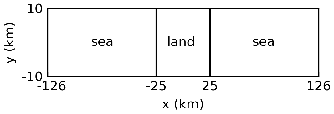
Figure 3 shows the domain configuration. A peninsula is located at the domain center. The sea is to the left and right sides of the peninsula. The width of the peninsula is 50 km, which is approximately the width of Leizhou Peninsula (Fig. 1). The domain is 252 km in the cross-coast direction (x direction hereafter), 20 km in the along-coast direction (y direction hereafter), and 17 km in the vertical direction (z direction hereafter). In the x direction, tests show that a length of ∼250 km is sufficient to accommodate the sea-breeze circulations; i.e., the lateral “open” boundary conditions do not affect the simulated sea-breeze circulations. In the y direction, tests show that a periodicity length of 20 km is large enough to capture the largest eddies because further increasing this length to 30 km produces similar results. The horizontal resolution is uniformly 100 m. The vertical resolution is 40 m from the surface to 4 km, then it gradually stretches to 200 m at 6.4 km, and then remains at 200 m up to the model top. The vertical resolution in this study is even higher than that in Antonelli and Rotunno (2007), where the sea-breeze circulation is reasonably well simulated. A Rayleigh damping layer is used above 13 km to absorb gravity waves. An adaptive time step is used, and the longest time step is 2 s.
Idealized surface fluxes are prescribed based on the ERA5 reanalysis data (Hersbach et al., 2020). For the sea surface, the Bowen ratio is 0.1, and the total heat flux (which is the sum of sensible heat flux and latent heat flux) is constant at 100 W m−2 during the considered time. For the land surface, the Bowen ratio is 0.2, and the total heat flux displays a prominent diurnal cycle. Therefore, the total heat flux is prescribed as
where THFm is the maximum total heat flux, and t is time. On the chosen day, the maximum total heat flux over the peninsula is 480 W m−2. However, during all of September 2018, the maximum total heat flux varies between 700 and 300 W m−2. Therefore, three values are tested here, i.e., 700, 500, and 300 W m−2. Hereafter, the three simulations are, respectively, referred to as THF700, THF500, and THF300. In addition, the roughness length is set to 0.1 m for the land surface and m for the sea surface (Wieringa, 1993).
Each simulation is run from t=0 to 12 h. The three-dimensional (3-D) fields were saved every 10 min. However, our initial analysis showed that the 10 min data could not resolve the DCI processes. Therefore, the model was restarted and the 3-D fields were saved every 1 min during the DCI period. In simulations THF700, THF500, and THF300, the 1 min data cover t=7.5 to 9.5 h, t=8.5 to 10.5 h, and t=10.5 to 12 h.
Online Lagrangian parcels were used to investigate the processes of DCI. The resolved-scale velocity is linearly interpolated to the position of the parcel, and the second-order Runge–Kutta method is used to update the position of the parcel. A similar method is used by Yang et al. (2015). Note that the subgrid-scale velocity is not considered in this calculation. Although including the subgrid-scale velocity may change the individual parcel trajectory (Weil et al., 2004; Yang et al., 2008), it does not change the statistics of a large number of parcel trajectories (Yang et al., 2008). The latter is the case in this study. Parcels were released at every grid point in the region of −10 km<x<10 km, −10 km<y<10 km, and 0 km<z<2 km. The total number of parcels is 2×10⁶. By restarting the simulations, we can release the parcels at different times. The release times will be mentioned in the appropriate sections.
Figure 4a–d show the pseudo albedo at four times in simulation THF700. The pseudo albedo is the parameterized albedo of the simulated clouds. It is calculated in order to compare the simulated clouds with the satellite-observed clouds (Zhang et al., 2005). Note that the Sun rises at t= 0 h in model time but at 06:00 in LST, so model time +6 h is LST. The four times in Fig. 4a–d correspond to the four times of Fig. 1a–d. Clouds do not develop over the sea in our simulations (not shown); thus, only the land part is shown in Fig. 4. A comparison of Figs. 1 and 4 indicates that the simulation qualitatively reproduces the observed evolution of the convection. At t=5 h, Fig. 4a shows that the clouds are small and disorganized. As time goes by (Fig. 4b and c), the cloud field shrinks and finally becomes a line of strong convective cells near the domain center (Fig. 4d). Figure 4e reveals that the cloud top of the strongest convective cell is higher than 12 km at t=8 h. Note that the cloud top is defined as the highest grid point with cloud water mixing ratio greater than 0.01 g kg−1. In addition, Fig. 4a–c also indicate that the convective cells near the edges of the cloud field, which are actually the positions of the sea-breeze fronts, are bigger than those between the two edges. This point will be revisited in Sect. 4.1.
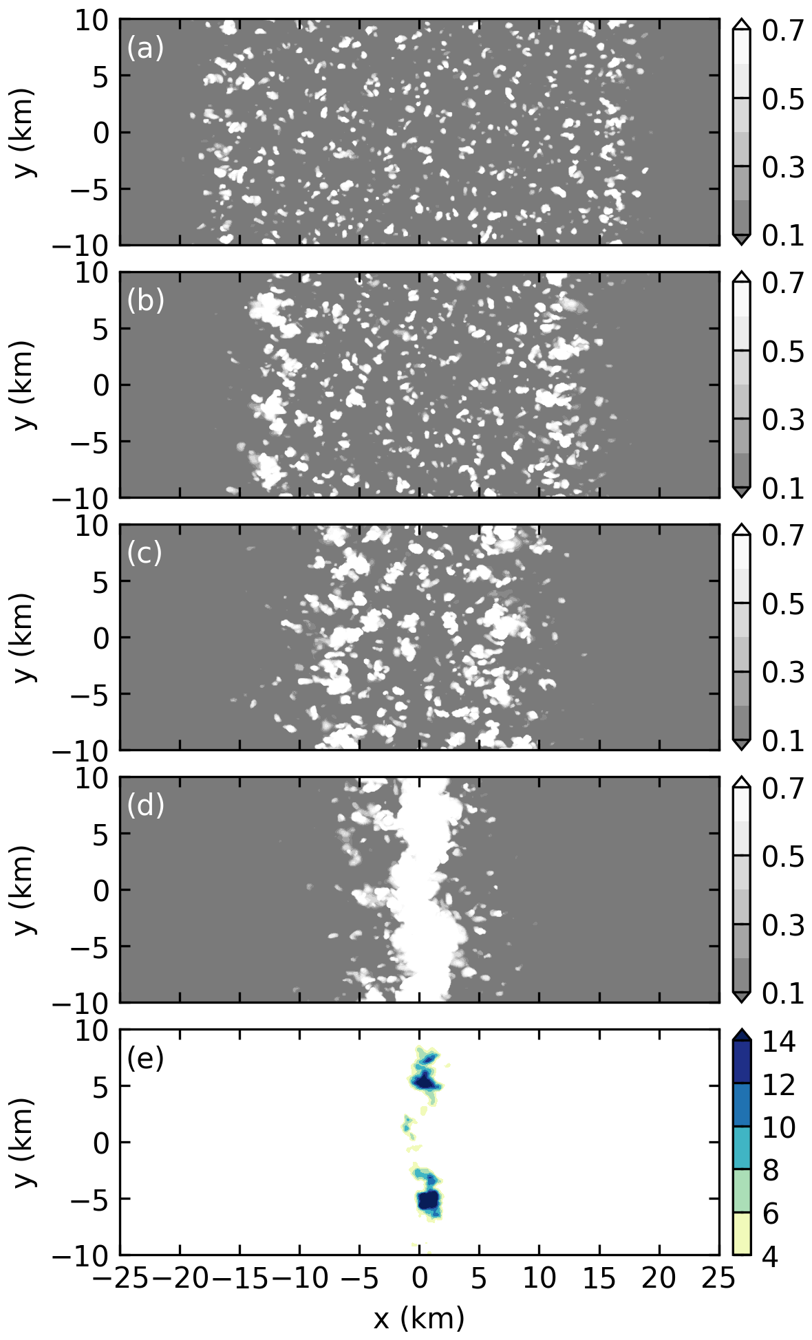
Figure 4Pseudo albedo in simulation THF700 at (a) t=5 h, (b) t=6 h, (c) t=7 h, and (d) t=8 h. (e) Cloud-top height (km) at t=8 h. Note that only the land part is shown.
The reanalysis data show that the maximum total heat flux is 480 W m−2 on the chosen day. However, a maximum total heat flux of 700 W m−2 is required for the model to reproduce the observed time of DCI. In simulations THF500 and THF300, the DCI is, respectively, delayed by 1 and 3 h. Several reasons may explain the difference in DCI time between the simulations and the observations. For example, Miller et al. (2003) pointed out that the environmental wind increases the low-level convergence associated with the sea-breeze front. Therefore, the omission of environmental wind may produce weaker sea-breeze fronts and hence postpone DCI. In addition, the omission of topography, the cyclic boundary condition in the y direction (i.e., the peninsula is infinite in the y direction), and the simplification of coastline shape may all contribute to the difference in DCI time between the simulations and the observations.
It is found that the effect of sea-breeze circulation on the preconvective environment is similar in all three simulations. Thus, only simulation THF700 is presented. As shown later, the effect of the sea-breeze circulation is different before and after the collision of sea-breeze fronts. These two periods are therefore discussed separately.
4.1 Before the collision of sea-breeze fronts
Figure 5 shows the y-averaged cross-coast wind, along-coast wind, potential temperature, vapor mixing ratio, convective available potential energy (CAPE), and convective inhibition (CIN) at t=6 h in simulation THF700. In this study, CAPE and CIN are calculated by lifting a parcel that possesses the mean properties of the lowest 0.2 km. Two sea-breeze circulations develop, with the left one around the left coast and the right one around the right coast (Fig. 5a). Weak mean winds also develop in the y direction due to the Coriolis effect (Fig. 5b). At t=6 h, the sea-breeze fronts have moved inland by 15 km (Fig. 5a). As the sea breeze moves inland, the sensible heat flux increases its potential temperature (Fig. 5c), and the latent heat flux increases its vapor mixing ratio (Fig. 5d). Therefore, CAPE increases while CIN decreases from the coast to the sea-breeze front (Fig. 5e and f). Figure 5f also indicates that CIN maximizes near the coasts. As found by Cuxart et al. (2014), this is because the return flow has a downward component near the coast, which produces subsidence warming and thereby stabilizes the atmosphere.
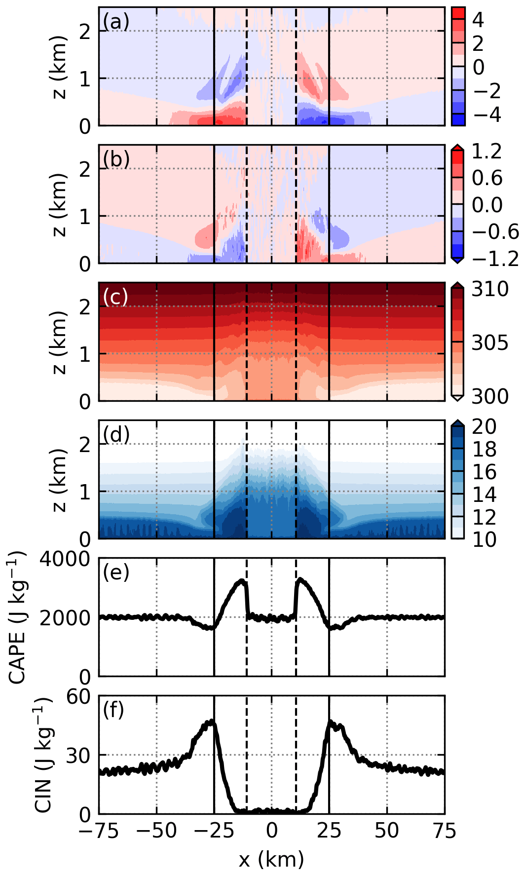
Figure 5y-averaged (a) cross-coast wind (m s−1), (b) along-coast wind (m s−1), (c) potential temperature (K), (d) vapor mixing ratio (g kg−1), (e) CAPE, and (f) CIN at t=6 h in simulation THF700. The solid lines at and 25 km denote the coasts. The dashed lines denote the identified positions of the sea-breeze fronts.
Between the two sea-breeze fronts, Fig. 5c indicates that the potential temperature is higher than that in the sea breeze. For the air between the sea-breeze fronts, it is always heated by the stronger sensible heat flux from the land surface, while for the air in the sea breeze it is first heated by the weaker sensible heat flux from the sea surface, and then heated by the stronger sensible heat flux from the land surface. Therefore, the air between the sea-breeze fronts receives more heat and is hence warmer than the air in the sea breeze. In addition, the large sensible heat flux between the sea-breeze fronts forces the boundary layer to grow rapidly, entraining a significant amount of dry air into the boundary layer. Therefore, the vapor mixing ratio between the sea-breeze fronts slowly decreases with time (not shown). At t=6 h, the vapor mixing ratio between the sea-breeze fronts is lower than that in the sea breeze (Fig. 5d). As a result, CAPE between the sea-breeze fronts is substantially smaller than that in the sea breeze (Fig. 5e). Figure 5f shows that CIN has been completely removed between the sea-breeze fronts. It is worth mentioning that although CAPE is large and CIN is nearly zero over a large portion of the land, deep convection does not develop at this time.
Thermal size plays an important role in determining DCI, as mentioned in Sect. 1. It is therefore interesting to investigate whether the thermal size is affected by the sea-breeze circulation. This is done by comparing the thermal sizes near the sea-breeze fronts to those between the sea-breeze fronts. The thermals within the sea breezes are small and weak (not shown) and are thus not analyzed. Due to the turbulent nature of the flow, it is probably not useful to investigate the size of individual thermals. Therefore, we, respectively, composite the thermals near the sea-breeze fronts and those between the sea-breeze fronts and then compare the sizes of the composite thermals.
Here, we briefly present the method of compositing. The details are given in Appendix B. First, we define the positions of the sea-breeze fronts. Second, we identify thermals and define the position of each thermal. Third, a thermal is defined as a “left-front thermal” if its distance from the left sea-breeze front is less than 1 km; a thermal is defined as a “right-front thermal” if its distance from the right sea-breeze front is less than 1 km; and a thermal is defined to be an “intermediate thermal” if it is between the two sea-breeze fronts and is more than 1 km away from each sea-breeze front. Fourth, a procedure similar to that used by Finnigan et al. (2009) and Schmidt and Schumann (1989) is used to composite the thermals at a given output time. Note that the three types of thermals are composited separately. Finally, the size and vertical velocity of the composite thermals are, respectively, non-dimensionalized by the boundary-layer height (zi) and the convective velocity scale (w*) and averaged over a period of time to give the mean composite thermal.
Figure 6 shows the mean composite left-front thermal, mean composite intermediate thermal, and mean composite right-front thermal averaged from t=5 h 30 min to 6 h 30 min. Figure 6a indicates that the mean composite left-front thermal tilts to the left; and Fig. 6e indicates that the mean composite right-front thermal tilts to the right. This tilting is why we composite the left-front thermal and the right-front thermal separately. Due to the convergence near the sea-breeze fronts, Fig. 6 shows that the mean composite thermals near the sea-breeze fronts are substantially larger than the mean composite intermediate thermal. Furthermore, the mean composite thermals near the sea-breeze fronts are moister than the mean composite intermediate thermal. The larger and moister thermals near the sea-breeze fronts explain the fact that the horizontal scales of the clouds near the sea-breeze fronts are bigger than those between the two sea-breeze fronts (Fig. 4).
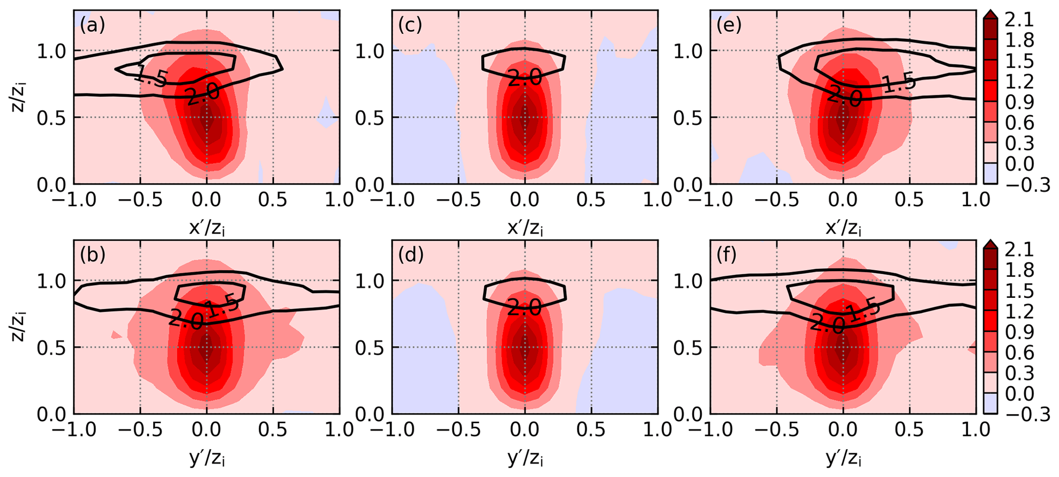
Figure 6(a) x–z cross section and (b) y–z cross section of the composite left-front thermal averaged from t=5 h 30 min to 6 h 30 min in simulation THF700. The filled contours indicate the non-dimensionalized vertical velocity, and the black contours indicate the dew point depression (K). Panels (c, d) are the same as (a, b) except for the composite intermediate thermal. Panels (e, f) are the same as (a, b) except for the composite right-front thermal.
Interestingly, Fig. 6 also shows that the vertical velocity of the mean composite thermals near the sea-breeze fronts is similar to that of the mean composite intermediate thermal. This suggests that, in the present simulation, the effect of a sea-breeze front is to increase the size of the thermal but not to strengthen the updraft of the thermal. Many previous studies showed that the updraft near the front of a gravity current is strengthened (e.g., Iwai et al., 2011); however, several observational studies indicate that the magnitude of updraft is not changed by boundary-layer convergence zones (e.g., Kraus et al., 1990; Wood et al., 1999). Hence, further studies are required to understand the effect of sea-breeze fronts on the magnitude of the thermal updrafts.
4.2 After the collision of sea-breeze fronts
Figure 7 shows the y-averaged cross-coast wind, along-coast wind, potential temperature, vapor mixing ratio, CAPE, and CIN at t=7 h 50 min in simulation THF700. Figure 7a shows that the two sea-breeze fronts have collided near the domain center. The potential temperature near the domain center is almost the same as that at t=6 h (cf. Figs. 5c and 7c). Figure 7d shows that the vapor mixing ratio near the domain center is much higher than that at t=6 h (cf. Figs. 5d and 7d) as a result of the sea breezes transporting vapor inland. Consequently, CAPE near the domain center becomes much higher than that at t=6 h (cf. Figs. 5e and 7e) and is greater than 3000 J kg−1 (Fig. 7e). Figure 7f shows that the distribution of CIN at t=7 h 50 min is similar to that at t=6 h, except that the portion with near-zero CIN becomes smaller.

After the collision of sea-breeze fronts, deep convection quickly develops, which does not allow us to composite the thermals. Figure 8a shows the horizontal cross section of vertical velocity at z=0.5zi and at t=7 h 50 min, and indicates that updrafts exist along most of y direction around x=0 km. In order to compare the vertical velocity at t=7 h 50 min to the mean composite thermals, the length and the vertical velocity are, respectively, non-dimensionalized by zi and w* and shown in Fig. 8b. At various places, the length of the non-dimensional updraft is greater than 2 in the x direction, comparable to the mean composite thermals near the sea-breeze fronts (cf. Fig. 6). In the y direction, the length of the non-dimensional updraft is much larger than that of the mean composite thermals near the sea-breeze fronts shown in Fig. 6b and f. Strictly speaking, the non-dimensional updraft in Fig. 8b should not be compared to the mean composite thermals in Fig. 6 because the former is an instantaneous cross section, while the latter is the mean of multiple thermals. Nevertheless, we think it is safe to conclude that the horizontal scale of the thermals after the collision is even larger than that before the collision. Thus, due to the higher CAPE and even bigger thermal, the environment after the collision of sea-breeze fronts is a more favorable environment for DCI.
As shown above, the deep convective cells align along the centerline of the domain and are mostly confined between and 2 km (Fig. 4d). Thus, the fields averaged from to 2 km include the information of all convective cells. By analyzing the 1 min instantaneous fields averaged from to 2 km (see Fu, 2021), it is clearly seen that DCI is not a one-step process; instead, DCI is accomplished through the development of multiple generations of convection. Here, we define the first generation of convection as the convective cells initiated solely by the sea-breeze fronts and the second generation of convection as the convective cells affected by the first generation of convection. Similarly, we can also define the third generation of convection. In simulations THF700 and THF500, three generations of convection can be identified. In simulation THF300, only one generation of convection develops. It is worth pointing out that each generation usually contains multiple convective cells, and these convective cells may not develop synchronously. Due to this complexity, subjectivity is unavoidable when identifying the different generations of convection. In this section, we use simulation THF700 to show the detailed processes involved in DCI.
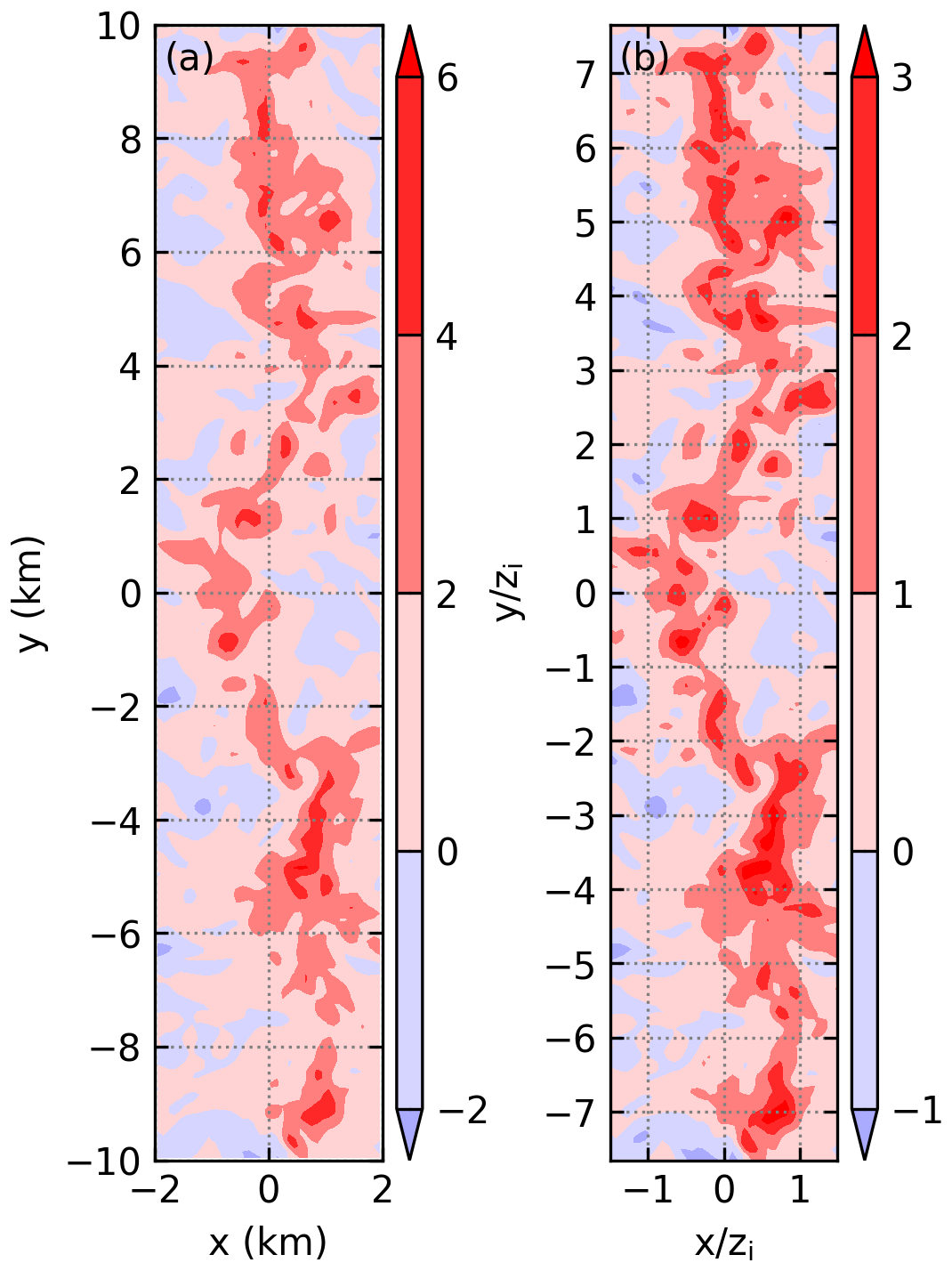
Figure 8Horizontal cross section of (a) dimensional vertical velocity (m s−1) and (b) non-dimensional vertical velocity at z=0.66 km and at t=7 h 50 min in simulation THF700.
Some definitions that are frequently used in this section are presented here. For a parcel that is initially below the LFC, it must be lifted by some lifting mechanism before it can ascend to LFC (Sect. 1). A parcel is defined as “having been lifted” if it is below the LFC at time t0, above the LFC at time t0+1 min, and ascends by more than 0.12 km from time t0 to t0+1 min (corresponding to a mean vertical velocity of 2 m s−1). We further define time t0 as the time when the parcel is lifted, and the position of the parcel at t0 as the position where the parcel is lifted.
We define a grid point to be within a cold pool if its surplus in density potential temperature (temperature surplus hereafter) satisfies
The density potential temperature , where θ is potential temperature, qv the vapor mixing ratio, qc the cloud water mixing ratio, qr the rain water mixing ratio, with Rd and Rv, respectively, the gas constants of dry air and vapor. The reference density potential temperature is the θρ averaged from to 10 km and from to 10 km at the start of the 1 min output. A column is defined to be within the cold pool if its lowest grid point satisfies Eq. (2). We search upward along the column and label the index of the first grid point not satisfying Eq. (2) as k; then the height of (k-1)th grid point is defined as the depth of the cold pool. The temperature surplus averaged over all the grid points below the kth grid point is defined as the mean temperature surplus of the column.
5.1 First generation of convection
Figure 9a shows the vertical velocity at z=0.88 km, which is the LFC averaged from to 1 km and from to 10 km right after the collision of sea-breeze fronts. Due to the collision of the oppositely moving sea-breeze fronts, a quasi-linear updraft develops around x=0 km (Fig. 9a). Parcels are released at t=7 h 35 min and tracked forward for 20 min to investigate where the first generation of convection develops. Figure 9b shows the number of parcels that are lifted at t= 7 h 47 min at each grid point. Inspection of Fig. 9a and b shows that the positions where the parcels are lifted are almost the same as the positions where the vertical velocity is greater than 2 m s−1. This is a direct result of the definition. Figure 9b also indicates that more parcels are lifted from regions with stronger updrafts (cf. Fig. 9a), similar to that found by Tang and Kirshbaum (2020).
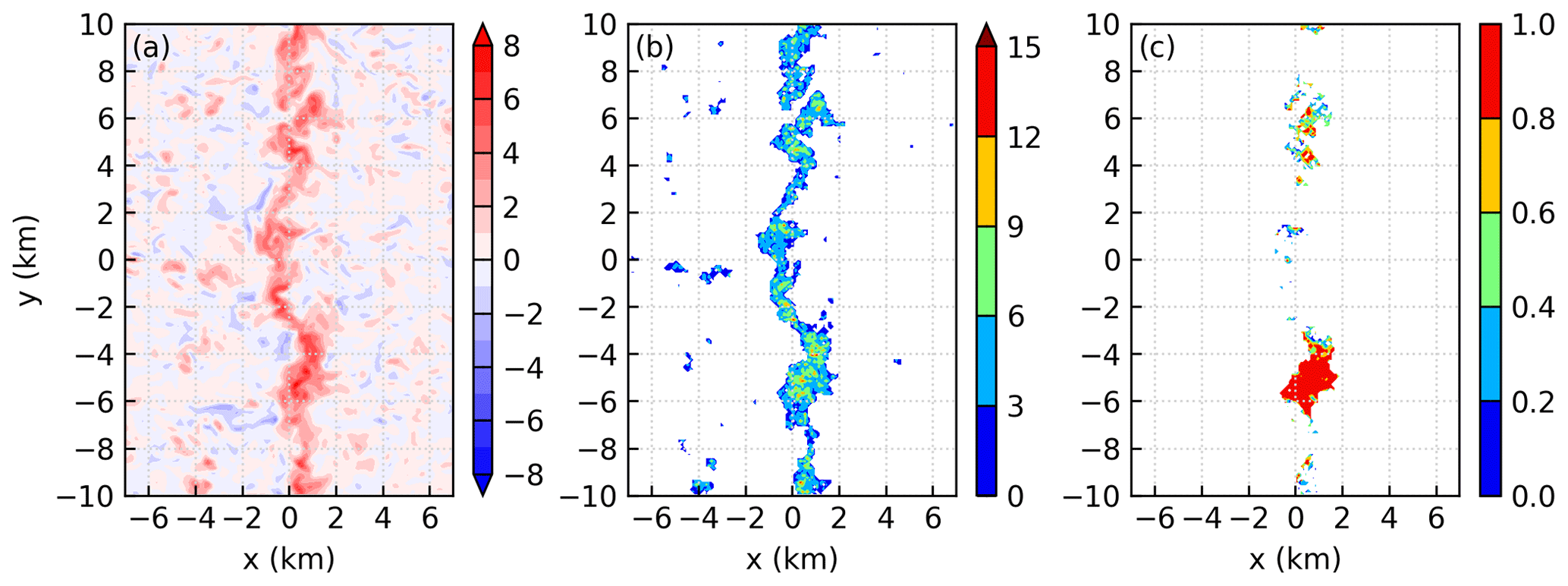
Figure 9(a) The vertical velocity at z=0.88 km. (b) The number of parcels that are lifted at each grid point. (c) The fraction of parcels that rise above 4 km in all parcels that are lifted. The parcels are released at t=7 h 35 min and tracked forward for 20 min. The results are at t=7 h 47 min of simulation THF700.
A critical height is used to distinguish the parcels that rise to high levels from the parcels that do not rise to high levels. The maximum height reached by the first generation of convection is approximately 6 km, as shown below. We therefore set the critical height to be 4 km. Figure 9c shows the fraction of parcels that rise above 4 km in all the parcels that are lifted at t= 7 h 47 min. Not all the parcels that are lifted manage to rise above 4 km. Furthermore, the parcels that rise above 4 km are mainly lifted from the regions where the updrafts are wider in the x direction. In this simulation, the updraft is nearly continuous in the y direction (Figs. 9a and 8). In this situation, the dimension in the y direction is not an appropriate measure of the updraft size, but the dimension in the x direction is an appropriate measure. Therefore, Fig. 9 suggests that convective cells developing from larger updrafts rise to higher levels, consistent with previous studies (e.g., Dawe and Austin, 2012; Rousseau-Rizzi et al., 2017). It is worth mentioning that at the time of Fig. 9, the convective cells are still below z=4 km (see Fu, 2021), so the wide updraft is mostly produced by the boundary-layer forcing and has not been substantially affected by the convective cell.
Figure 10a–c, respectively, show the vertical velocity, cloud water mixing ratio, and rain water mixing ratio averaged from to 2 km at t=7 h 56 min. The mean vertical velocity is defined as , where f(w)=1 if w>0 and f(w)=0 if w≤0. N is the number of grid points between to 2 km, either with w>0 or ≤0, so the number of grid points going into the averaging procedure is fixed. The two convective cells around and 5 km in Fig. 10a correspond to the two clusters of parcels that rise above 4 km (cf. Fig. 9c). They are produced directly through the collision of sea-breeze fronts and hence belong to the first generation of convection. At this time, these two convective cells have reached their mature stages and the cloud tops are close to their maximum heights. Cloud water forms as a result of the strong updrafts (Fig. 10b). Through a series of cloud microphysical processes (Fu et al., 2019), rain water forms around and 5 km (Fig. 10c).

Figure 10(a) Vertical velocity (m s−1), (b) cloud water mixing ratio (g kg−1), and (c) rain water mixing ratio (g kg−1) averaged from to 2 km at t=7 h 56 min in simulation THF700.
The rain shafts around , 0, and 10 km are produced by the earlier convective cells, which also belong to the first generation of convection but develop several minutes earlier than the convective cells around and 5 km. In addition, it is found that the convective cell around km is the strongest in the first generation of convection, and its position along the colliding sea-breeze fronts seems to be random. A detailed analysis indicates that the randomness is related to the variability of the sea-breeze fronts in the y direction (not shown). We note that because of the cyclic boundary condition in the y direction, the rain shafts around and 10 km are actually produced by the same convective cell. Similar caution should be used when interpreting other variables.
5.2 Second generation of convection
Figure 11a and b, respectively, show the depth and the temperature surplus of the cold pools at t=8 h. Four cold pools can be identified, corresponding to the four rain shafts in Fig. 10c. At this time, the cold pools have not yet merged and are generally shallower than 0.2 km and warmer than −2 K near their edges.
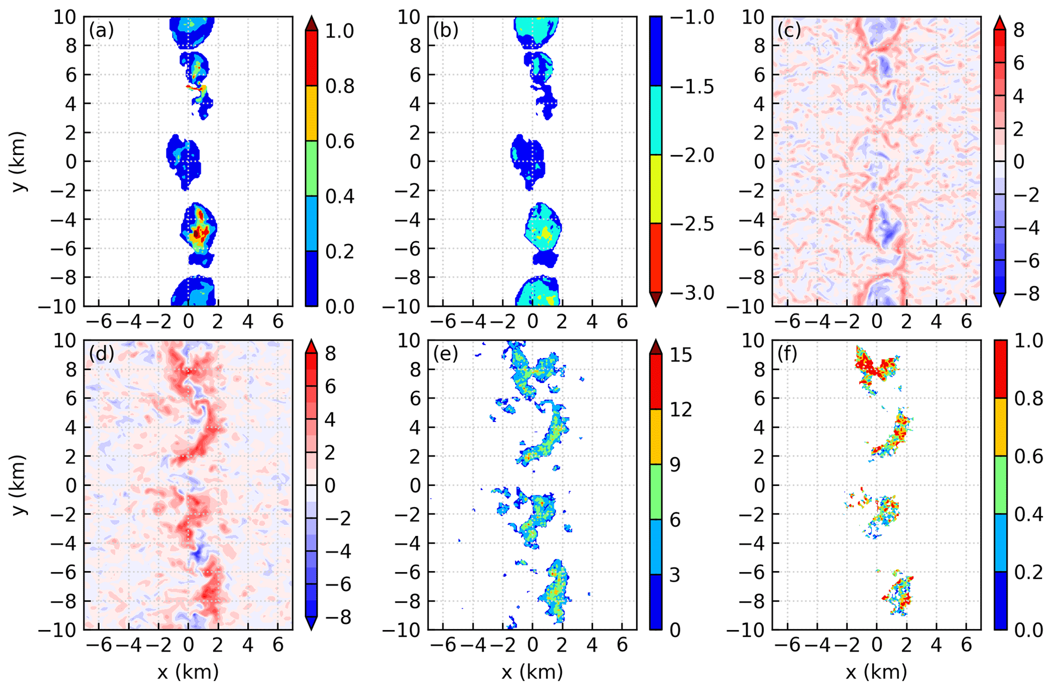
Figure 11Panels (a) and (b) are, respectively, the depth (km) and temperature surplus (K) of the cold pools. Panels (c) and (d) are, respectively, the vertical velocity at z=0.2 and 0.88 km. (e) The number of parcels that are lifted at each grid point. (f) The fraction of parcels that rise above 6 km in all parcels that are lifted. The parcels are released at t=7 h 55 min and tracked forward for 25 min. The results are at t=8 h of simulation THF700.
Figure 11c and d, respectively, show the vertical velocity at z= 0.2 and 0.88 km. At z=0.2 km, downdrafts exist in the interiors of the cold pools. Closed rings of updraft can be seen near the edges of the cold pools. At z=0.88 km, downdrafts are also discernable at the centers of the cold pools. However, updrafts do not form closed rings; instead, four updrafts are produced. Figure 11d also shows that the updrafts are separated by the downdrafts. A comparison of Fig. 11c and d reveals that some updrafts are deep because they are seen at both z=0.2 and 0.88 km, while the other updrafts are shallow because they are seen at z=0.2 km but not at z=0.88 km. The formation of deep and shallow updrafts will be further explored below. Note that at the time for Fig. 11, the convective cells of the second generation are mostly below z=4 km (see Fu, 2021), so the wide updrafts shown in Fig. 11d are also mostly produced by the boundary-layer forcing and are not substantially affected by the convective cells, similar to the first generation of convection.
Parcels are released at t=7 h 55 min and tracked forward for 25 min to investigate the development of the second generation of convection. Figure 11e shows that parcels are lifted from the regions with vertical velocity greater than 2 m s−1 (cf. Fig. 11d), similar to that observed in Fig. 9. The second generation of convection is stronger than the first generation, as seen below. We accordingly use a higher critical height, i.e., 6 km, to distinguish the parcels that rise to high levels from the parcels that do not rise to high levels. The fraction of parcels that rise above 6 km is shown in Fig. 11f. Each updraft produces some parcels that rise above 6 km. At the time shown in Fig. 11f, the fraction of parcels that rise above 6 km is generally small for each updraft. However, the fraction will increase to over 0.8 in the following 8 min (not shown).
Figure 12a and c, respectively, show the vertical cross section of cross-coast wind and vertical velocity at km. The black contour indicates the edge of the cold pool. At this time, the cold pool spans from to 0.8 km and is generally shallower than 0.2 km. The sea breezes experience weak lifting when they encounter the shallow gust fronts (Fig. 12a). After being lifted, the sea breezes continue to move and collide with each other, producing a wide and deep updraft (Fig. 12c). Obviously, the dominant forcing mechanism of the updraft is the collision of the sea-breeze fronts rather than the collision between the gust fronts and the sea-breeze fronts. In fact, this vertical cross section is representative of all regions where deep updrafts are produced. In particular, in regions not covered by cold pools, the collision of sea-breeze fronts is the only forcing mechanism that produces the updraft.
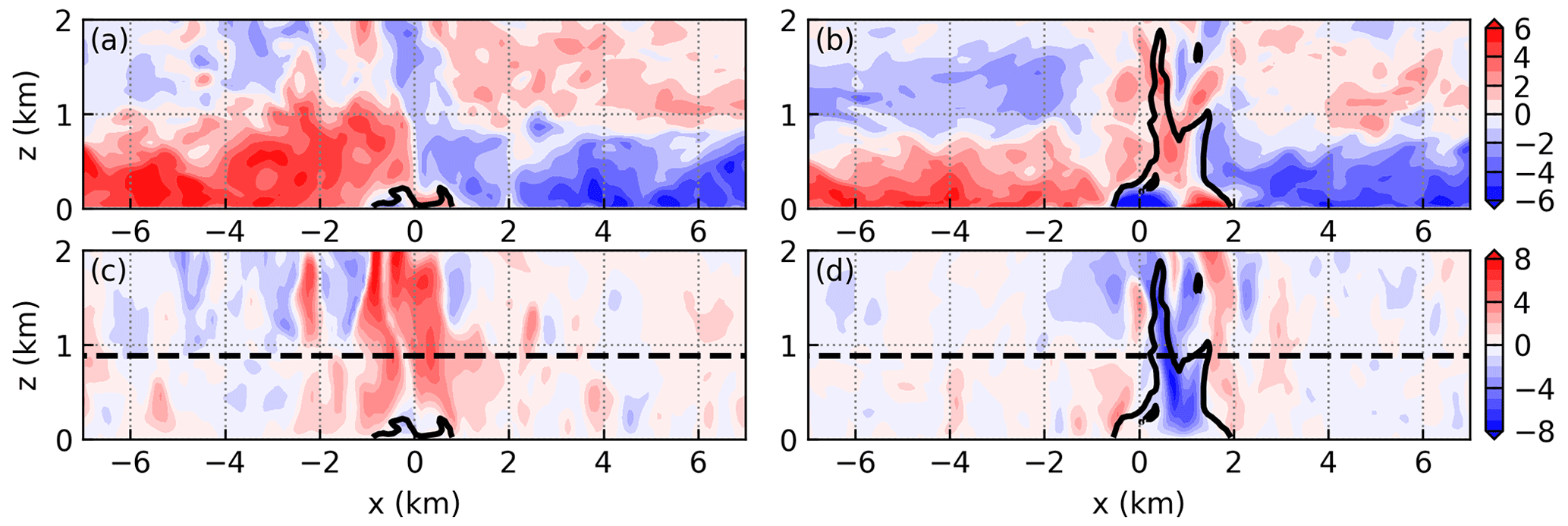
Figure 12Vertical cross section of (a) cross-coast wind and (c) vertical velocity at km. Panels (b) and (d) are, respectively, the same as (a) and (c) except at km. The black contour indicates the edge of the cold pool. The dashed line indicates the LFC. The results are at t=8 h of simulation THF700.
Figure 12b and d show the vertical cross section at km. This vertical cross section is representative of the regions where only shallow updrafts are produced. The cold pool is readily seen in Fig. 12b. The cold-pool depth near the edge is approximately 0.2 km, which is rather shallow. The updraft forced by the gust front is also shallow (Fig. 12d). More importantly, although the sea breezes that are lifted by the gust fronts continue to move toward each other and collide around x=1 km (Fig. 12b), deep updraft is produced. This is because the downdraft from aloft suppresses the development of updraft.
We can now summarize the processes through which the second generation of convection is produced. In the regions where downdrafts exist, deep updrafts cannot be produced because of the suppression effect exerted by the downdrafts produced by the first generation of convection. As a result, new convection does not develop in these regions. In the regions where downdrafts do not exist, the collision of sea-breeze fronts produces deep and wide updrafts. The second generation of convection therefore develops from these regions.
Figure 13a–c, respectively, show the y–z plots of the vertical velocity, cloud water mixing ratio, and rain water mixing ratio averaged from to 2 km at t=8 h 13 min. Figure 13a reveals multiple convective cells, corresponding to the clusters of parcels that rise above 6 km (cf. Fig. 11f). The animation of y–z plots (see Fu, 2021) reveals that the second generation of convection eventually rises above 10 km. These convective cells produce more cloud water (Fig. 13b) and consequently more rain water (Fig. 13c) than the first generation of convection.
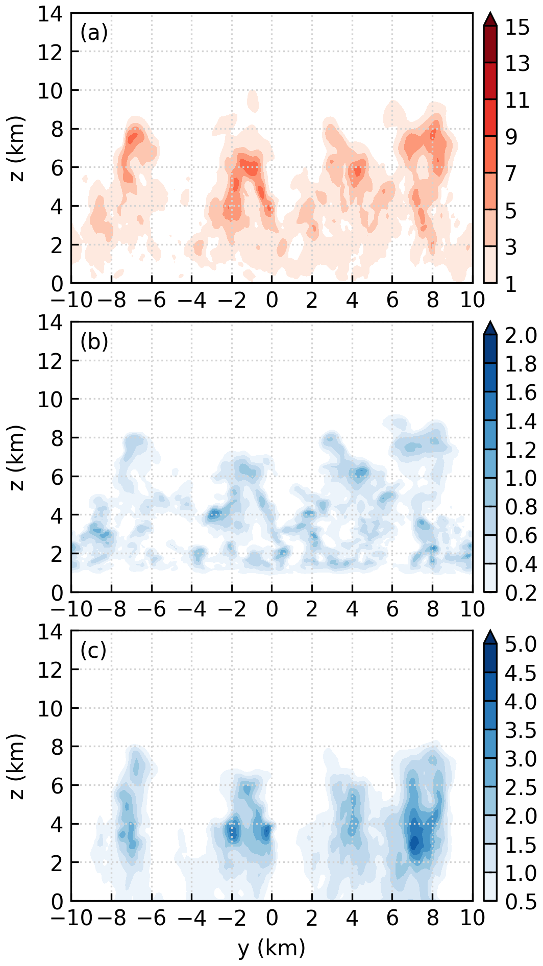
Three factors contribute to the result that the second generation of convection is deeper than the first generation of convection. First, the updrafts that produce the second generation of convection are more organized and are generally wider in the x direction than the updrafts that produce the first generation (cf. Figs. 9a and 11d). Second, the two convective cells between x=2 and 10 km are very close to each other (Fig. 13a). They might invigorate each other by moistening the environment, as suggested by Böing et al. (2012). Third, the first generation of convection moistens the troposphere below z=6 km. This reduces the dilution of the subsequent convective cells and hence tends to invigorate the second generation of convection. This point is supported by a sensitivity test, where the vapor mixing ratio of the non-cloudy grid points is strongly nudged to the mean vapor mixing ratio averaged from to 2 km and from to 10 km at 7 h 30 min. A grid point is defined as non-cloudy if its sum of cloud water and rain water mixing ratio is less than 0.01 g kg−1. The nudging is applied only for z>2 km. The sensitivity test (not shown) shows that the second generation of convection is only slightly stronger than the first generation of convection.
5.3 Third generation of convection
Figure 14a and b, respectively, show the depth and the temperature surplus of the cold pool at t= 8 h 17 min, when the cloud top of the third generation is near z=4 km (see Fu, 2021). It reveals a single cold pool that spans the whole y direction. This cold pool is generally deeper and colder than the cold pools at t=8 h (cf. Figs. 11 and 14). A careful examination of Fig. 14b reveals that the cold pool is not homogeneous but composed of two cold pools that are separated by the warmer regions (indicated by the blue color) around y=1 and 10 km. This conclusion is further confirmed by the inspection of the evolution of cold pools (see Fu, 2021). The collision of these two cold pools produces several intersection points. The most prominent intersection points are at and (2, 10) km.
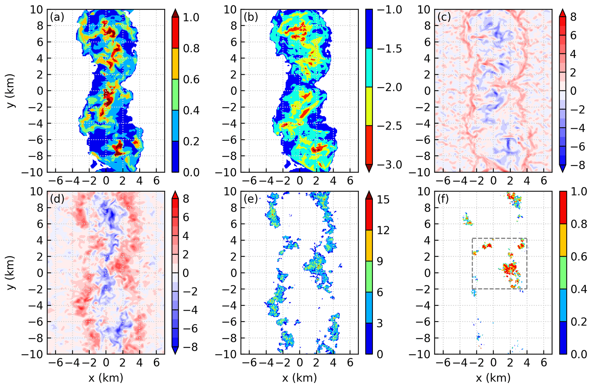
Figure 14Panels (a) and (b) are, respectively, the depth (km) and temperature surplus (K) of the cold pools. Panels (c) and (d) are, respectively, the vertical velocity at z=0.2 and 0.88 km. (e) The number of parcels that are lifted at each grid point. (f) The fraction of parcels that rise above 8 km in all parcels that are lifted. The gray rectangle encloses the parcel clusters that merge. The parcels are released at t=8 h 5 min and tracked forward for 40 min. The results are at t=8 h 17 min of simulation THF700.
Figure 14c and d, respectively, show the vertical velocity at z=0.2 and 0.88 km. Downdrafts can been seen in the interiors of the cold pools, both at z=0.2 and 0.88 km. At z=0.2 km, updrafts are produced at the edges of the cold pools and are nearly continuous. However, the updrafts at z=0.88 km are broken at various places. This means that some updrafts are deep while the other updrafts are shallow, similar to what we have seen at t=8 h. However, the mechanism that produces deep updrafts at t=8 h 17 min is different from that at t=8 h, as presented below. Furthermore, Fig. 14d reveals that the updrafts at the intersection points are wider in the x direction than the updrafts in other regions. This phenomenon is also seen in previous studies (e.g., Bai et al. 2019).
The parcels that are used to investigate the development of the third generation of convection are released at t=8 h 5 min and tracked forward for 40 min. Figure 14e shows that parcels are lifted from the regions with vertical velocity greater than 2 m s−1. For the third generation of convection, we use a critical height of 8 km to distinguish the parcels that rise to high levels from the parcels that do not rise to high levels. Figure 14f indicates that most of the parcels that rise above 8 km are lifted from the two intersection points; only a small number of parcels that rise above 8 km are lifted from regions other than the two intersection points.
Figure 15a and c, respectively, show the vertical cross section of cross-coast wind and vertical velocity at y=6.55 km at t=8 h 17 min. Near their edges, the depths of the cold pool are comparable to those of the sea breezes. In this situation, it is the collisions between the gust fronts and the sea-breeze fronts (Fig. 15a), instead of the collision of the sea-breeze fronts (cf. 12a), that produce the deep updrafts (Fig. 15c). Actually, deep updrafts are produced near almost all edges where the cold pool is deeper than 0.4 km (cf. Fig. 14a and d).
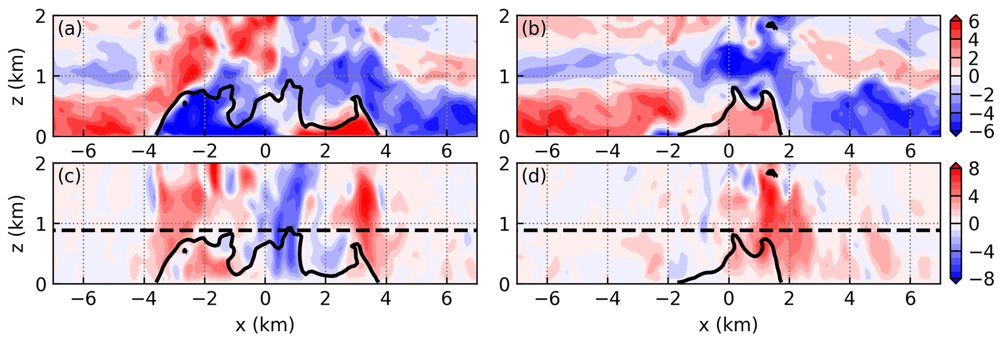
Figure 15Vertical cross section of (a) cross-coast wind and (c) vertical velocity at y=6.55 km. Panels (b) and (d) are the same as (a) and (c) except at y=0.75 km. The black contour indicates the edge of the cold pool. The dashed line indicates the LFC. The results are at t=8 h 17 min of simulation THF700.
Figure 15c also shows that the left updraft is farther away from the downdraft than the right updraft. In the following 20 min, some of the parcels lifted by the left updraft do not encounter strong downdrafts (Fig. 14f), so the convective cells developing from the left updraft rise above 8 km. However, the parcels that are lifted from the right updraft are quickly entrained into the downdrafts (not shown), so the convective cells developing from the right updraft quickly dissipate.
Figure 15b and d show the vertical cross section at y=0.75 km, which is close to the intersection point at km. The cold pool depth is approximately 0.7 km near the right edge (Fig. 15b). A deep updraft is produced through the collision between the gust front and the sea-breeze front (Fig. 15d). Figure 15d also shows that the updraft at y=0.75 km is much wider than that at y=6.55 km (cf. Fig. 15c), as mentioned above. Furthermore, the updraft shown in Fig. 15d is away from any major downdrafts, so the parcels lifted by it do not encounter strong downdrafts in the following 20 min. Thus, the convective cells developing from the intersection points manage to rise above 8 km.
Another factor is found to invigorate the third generation of convection. In the regions enclosed by the gray rectangle (Fig. 14f), there are multiple clusters of parcels that rise above 8 km, indicating that multiple convective cells are produced. Parcel trajectory analysis reveals that these convective cells merge with each other (not shown). As mentioned in Sect. 1, the merger of convective cells reduces the detrimental effect of entrainment, so the convective cells that merge rise to higher levels than the convective cells that do not merge.
We now summarize the processes through which the third generation of convection is produced. Two cold pools are produced by the second generation of convection. Near the intersection points of the cold pools, deep and wide updrafts are produced through the collision between the gust front and the sea-breeze front, and these updrafts are generally away from the major downdrafts produced by the second generation of convection. Therefore, convective cells develop from these deep and wide updrafts. Besides, minor convective cells also develop from regions other than the intersection points. Furthermore, the convective cells that are close to each other merge, consequently producing a deep convective cell.
Figure 16a–c, respectively, show the y–z plots of the vertical velocity, cloud water mixing ratio, and rain water mixing ratio averaged from to 2 km at t=8 h 35 min. The cloud top has reached the height of 13 km. Such a strong convective cell produces even more cloud water (Fig. 16b) and rain water (Fig. 16c) than the second generation of convection.
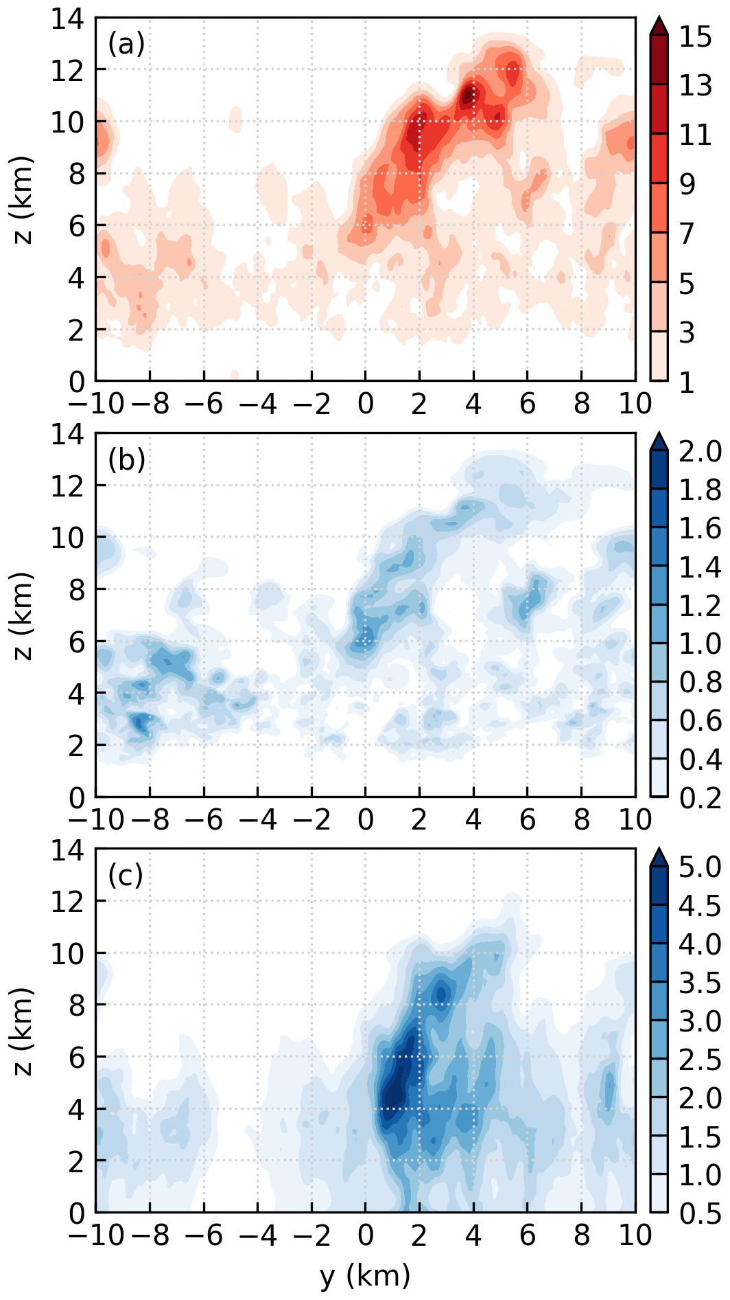
There are also three factors contributing to the result that the third generation of convection is stronger than the second generation of convection. First, it has been shown that the updrafts producing the third generation of deep convection are wider than those producing the second generation (cf. Figs. 11 and 14). Second, the merger of convective cells invigorates the third generation of convection. Third, the moistening effect by the first two generations of convection further promotes the development of the third generation of convection. In the sensitivity test where the vapor mixing ratio of the non-cloudy grid points is strongly nudged, the third generation of convection is only slightly stronger than the second generation of convection, which is only slightly stronger than the first generation of convection.

Figure 17(a) Number, (b) mean size (km), and (c) mean temperature surplus (K) of the convective cells in simulation THF700. Note that a logarithmic scale is used in panel (a). Panels (d–f) and (g–i) are the same as (a–c) except for simulations THF500 and THF300. The black, green, and red ellipses indicate the first, second, and third generations of convection, respectively.
Before discussing the difference among the three simulations, we tabulate two important parameters in Table 1. The first is zi, which is known to scale with the depth of the sea breeze (Antonelli and Rotunno, 2007). The second is a horizontal velocity scale (U). Similar to Antonelli and Rotunno (2007), it is defined as , where Ul and Ur are, respectively, the maximum wind speed of the y-averaged cross-coast wind at the left and right coasts. We note that zi and U are calculated at the last 10 min output time before the collision of sea-breeze fronts. As expected, Table 1 indicates that the sea breeze becomes shallower and slower as total heat flux decreases.
Figure 17 shows the number, mean horizontal size, and mean temperature surplus of the convective cells in each simulation. At each height, a grid point is defined as within a convective cell if its vertical velocity is greater than a threshold of 10 m s−1. Tests show that using a threshold of 5 or 15 m s−1 gives qualitatively the same results. These grid points are then four-way connected to form clusters, and each cluster is defined as a convective cell. The size of the convective cell , where A is the area of the convective cell. Note that the mean size of the convective cells is the size averaged over all convective cells, while the mean temperature surplus is the temperature surplus averaged over all grid points identified as within the convective cells. In addition, the ellipses in Fig. 17 indicate different generations of convection.
In simulations THF700 and THF500, there are more than 10 convective cells below z=4 km (Fig. 17a and d), and their mean size is less than 0.4 km (Fig. 17b and e). Above z=4 km, the number of convective cells generally decreases with height (Fig. 17a and d), while the mean size of the convective cells generally increases with height (Fig. 17b and e). Two factors contribute to this phenomenon: first, the small convective cells dissipate during their ascent and only the big convective cells rise to high levels; second, mergers occur among some convective cells. In addition, the convective cells are always positively buoyant above z=4 km (Fig. 17c and f), indicating that they are resistant to the detrimental effect of entrainment.
Table 1Boundary-layer height (zi) and the horizontal velocity scale (U).
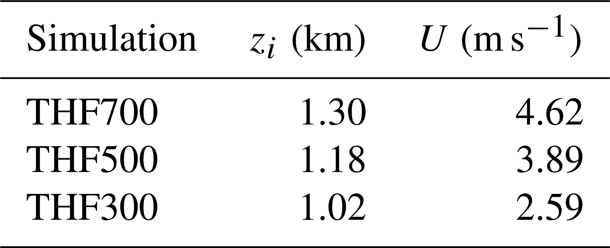
Figure 17a–c show that the later generation of convection is stronger than the earlier generation of convection in simulation THF700, as explained in Sect. 5. In simulation THF500, the development of the three generations of convection is generally similar to that in simulation THF700, so the later generation of convection is also stronger than the earlier generation of convection. However, because the sea breezes are shallower and slower (Table 1), the forcing of the first and second generations of convection is weaker in simulation THF500. As a result, the first and second generations of convection in simulation THF500 are both weaker than their counterparts in simulation THF700. Furthermore, the weaker second generation of convection produces shallower cold pools. The forcing of the third generation of convection is therefore weaker. As a result, the third generation of convection in simulation THF500 is also weaker than in simulation THF700. In simulation THF300, the sea breezes are even weaker, so only a few weak convective cells are produced (Fig. 17g–i).
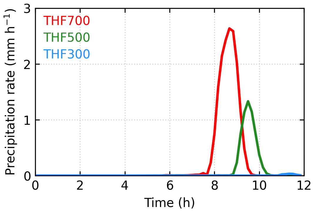
Figure 18 shows the mean surface precipitation rates over the land part for the three simulations. In simulation THF700, the sea-breeze fronts collide at t=7 h 50 min. Before the collision, negligible surface precipitation is produced; after the collision, a large surface precipitation rate is produced as a result of the successive developments of convection. In simulation THF500, the two sea-breeze fronts collide at t=8 h 50 min, which is 1 h later than that in simulation THF700. This is because decreasing sensible heat flux reduces the propagation speed of the sea-breeze fronts (Antonelli and Rotunno, 2007). Due to the weaker convection, a smaller surface precipitation rate is produced in simulation THF500 than in simulation THF700. In simulation THF300, the sensible heat flux is even smaller, so the sea-breeze fronts move even more slowly and collide at t=10 h 50 min. Negligible surface precipitation is produced in this simulation.
A series of large-eddy simulations are performed to investigate the processes involved in deep-convection initiation (DCI) over a peninsula. In each simulation, two sea-breeze circulations develop, with the two sea-breeze fronts moving inland. When the sea-breeze fronts collide near the centerline of the domain, CAPE is substantially increased due to the vapor transported by the sea breezes and the surface heating, and strong updrafts are produced due to the collision of sea-breeze fronts.
DCI occurs after the collision of sea-breeze fronts. In the simulations with a maximum total heat flux of 700 and 500 W m−2, DCI occurs through the development of three generations of convection. The first generation of convection develops as a direct result of the sea-breeze-front collisions, and the position of the first generation of convection along the colliding sea-breeze fronts is random. The second generation of convection is also produced mainly through the collision of sea-breeze fronts, and the collision between the gust fronts and the sea-breeze fronts plays a minor role. The position of the second generation of convection is affected by the first generation of convection: the second generation of convection does not develop in regions where strong downdrafts are produced by the first generation of convection but instead develops in regions where no strong downdrafts are produced. The third generation of convection mainly develops from the intersection points of the cold pools that are produced by the second generation of convection. Near the intersection points, the updrafts are deep and wide, and no major downdraft is present. Parcels lifted from regions other than the intersection points also play a minor role in producing the third generation of convection. In addition, merger occurs to convective cells that are close to each other, further invigorating the third generation of convection. A sensitivity test shows that the moistening effect by the earlier convection also promotes the development of the later convection.
As the total heat flux decreases from 700 to 500 W m−2, both the height and speed of the sea breezes are reduced, so the forcing of the first and second generations of convection is reduced. These two generations of convection are therefore weaker. Furthermore, the weaker second generation of convection produces shallower cold pools, reducing the forcing of the third generation. Consequently, the third generation of convection is also weaker. As the total heat flux further decreases to 300 W m−2, the sea breezes are even shallower and weaker. Only one generation of shallow convection is produced.
Simulation THF500 is rerun using the Morrison two-moment microphysics scheme. We perform a sensitivity test on simulation THF500 instead of THF700, because the maximum total heat flux over the peninsula is approximately 500 W m−2 on the chosen day. There are two major differences between the simulation using the Morrison scheme and that using the Kessler scheme. The first difference is that the peak strength of convection in the simulation using the Morrison scheme is stronger than that in the simulation using the Kessler scheme. This is due to the slower development of precipitation, which postpones the development of downdrafts, and the extra heating from the freezing processes, which increases the buoyancy of the clouds. The second difference is that there are only two generations of convection in the simulation using the Morrison scheme, while there are three generations of convection in the simulation using the Kessler scheme. This is probably because CAPE has been consumed by the end of the stronger second generation in the simulation using the Morrison scheme. Nevertheless, detailed analysis shows that the development of the two generations of convection in the simulation using the Morrison scheme is similar to the first two generations of convection in the simulation using the Kessler scheme.
Before performing the compositing, we need to define the positions of sea-breeze fronts. Because the simulation setup is nearly homogeneous in the y direction, we only need to define the positions of sea-breeze fronts in the x direction. First, the cross-coast wind at the lowest level (z=0.02 km) is averaged along the y direction. Then, a running average is performed to remove the effects of turbulence. By trial and error, we find that performing the running average twice to the y-averaged cross-coast wind gives the best result. The window for running average is 5 km. Finally, the location having the maximum horizontal convergence in the left half of the domain is defined as the position of the left sea-breeze front; the location having the maximum horizontal convergence in the right half of the domain is defined as the position of the right sea-breeze front.
We also need to define the position of each thermal. Similarly, we only define the position of a thermal in the x direction. On a reference horizontal plane at z=0.5zi, any grid point with vertical velocity greater than 1.5 w* is defined as within a thermal. Here, the boundary-layer height zi is defined as the height of the lowest grid point with K km−1, where is the potential temperature averaged from to 1 km and to 10 km. The convective velocity scale w* is defined as
where g is the gravitational acceleration, and is the turbulent flux of potential temperature at the surface. All grid points that are identified as within a thermal are then four-way connected in the horizontal plane to form clusters. Each cluster is defined as a thermal. The mean x coordinate of all grid points within the thermal is defined as the position of the thermal. According to the distance between the thermal and the sea-breeze front, a thermal is further categorized as a left-front thermal, a right-front thermal, or an intermediate thermal, as described in Sect. 4.1.
A procedure similar to that used by Finnigan et al. (2009) and Schmidt and Schumann (1989) is used to composite the thermals at a given output time. As an example, we detail the procedure of compositing the left-front thermals. First, for each left-front thermal, we find the grid point having the maximum vertical velocity in the plane at z=0.5zi. The positions of these grid points are labeled as (xm, ym)i, where i is the index of the left-front thermals. Note that each (xm, ym)i indicates a 3-D thermal. Then, all the left-front thermals are shifted horizontally so that all (xm, ym)i coincide. A new coordinate system is therefore established where the coincident (xm, ym) is at (0, 0). Finally, ensemble averaging is performed over all the left-front thermals, giving rise to the composite left-front thermal at the output time. By repeating this procedure, we can obtain the composite left-front thermals at all output times.
We also need to average the composite left-front thermals over a certain period of time. Because the boundary layer is deepening, the thermal size tends to increase with time. In addition to the boundary-layer height, the sensible heat flux is also evolving, so the updraft strength also varies with time. In this situation, the size and vertical velocity of the composite thermal are, respectively, non-dimensionalized by zi and w* before they are averaged over time. The same procedure is used to calculate the mean composite right-front thermal and mean composite intermediate thermal.
Please contact Shizuo Fu for the details of the model setup and model output data. Figures showing the 1 min instantaneous fields can be downloaded from https://doi.org/10.17605/OSF.IO/JZETH (Fu, 2021).
SF and RR designed the study. SF performed the simulations and analyzed the results. All authors commented on the results and co-wrote the paper.
The authors declare that they have no conflict of interest.
The research product of L1 gridded data (produced from Himawari-8) that was used in this paper was supplied by the P-Tree System, Japan Aerospace Exploration Agency (JAXA). The sounding data were downloaded from http://weather.uwyo.edu/upperair/sounding.html (last access: 6 June 2019). ERA5 data were generated using Copernicus Climate Change Service Information (2019). We thank George Bryan for providing and helping us with the CM1 model, and Edward Patton for useful comments.
This research has been supported by the National Natural Science Foundation of China (grant nos. 41930968, 42075067, and 42005059). The visit of Shizuo Fu to the National Center for Atmospheric Research is supported by the China Scholarship Council. The National Center for Atmospheric Research is sponsored by the National Science Foundation.
This paper was edited by Holger Tost and reviewed by Daniel Kirshbaum and one anonymous referee.
American Meteorological Society: Dryline, Glossary of Meteorology, available at: http://glossary.ametsoc.org/wiki/dryline, last access: 20 December 2020a.
American Meteorological Society: Gust front, Glossary of Meteorology, available at: http://glossary.ametsoc.org/wiki/gust_front, last access: 20 December 2020b.
Antonelli, M. and Rotunno, R.: Large-eddy simulation of the onset of the sea breeze, J. Atmos. Sci., 64, 4445–4457, https://doi.org/10.1175/2007jas2261.1, 2007.
Arnott, N. R., Richardson, Y. P., Wurman, J. M., and Rasmussen, E. M.: Relationship between a weakening cold front, misocyclones, and cloud development on 10 June 2002 during IHOP, Mon. Weather Rev., 134, 311–335, https://doi.org/10.1175/MWR3065.1, 2006.
Bai, L., Meng, Z., Huang, Y., Zhang, Y., Niu, S., and Su, T.: Convection Initiation Resulting From the Interaction Between a Quasi-Stationary Dryline and Intersecting Gust Fronts: A Case Study, J. Geophys. Res.-Atmos., 124, 2379–2396, https://doi.org/10.1029/2018JD029832, 2019.
Bai, L., Chen, G., and Huang, L.: Convection Initiation in Monsoon Coastal Areas (South China), Geophys. Res. Lett., 47, e2020GL087035, https://doi.org/10.1029/2020GL087035, 2020.
Beringer, J., Tapper, N. J., and Keenan, T. D.: Evolution of maritime continet thunderstorms under varying meteorological conditions over the Tiwi Islands, Int. J. Climatol., 21, 1021–1036, https://doi.org/10.1002/joc.622, 2001.
Birch, C. E., Parker, D. J., Marsham, J. H., Copsey, D., and Garcia-Carreras, L.: A seamless assessment of the role of convection in the water cycle of the west African Monsoon, J. Geophys. Res.-Atmos., 119, 2890–2912, https://doi.org/10.1002/2013JD020887, 2014.
Birch, C. E., Roberts, M. J., Garcia-Carreras, L., Ackerley, D., Reeder, M. J., Lock, A. P., and Schiemann, R.: Sea-breeze dynamics and convection initiation: The influence of convective parameterization in weather and climate model biases, J. Climate, 28, 8093–8108, https://doi.org/10.1175/JCLI-D-14-00850.1, 2015.
Blanchard, D. O. and Lopez, R. E.: Spatial patterns of convection in South Florida, Mon. Weather Rev., 113, 1282–1299, https://doi.org/10.1175/1520-0493(1985)113<1282:SPOCIS>2.0.CO;2, 1985.
Bluestein, H. B.: Surface Boundaries of the Southern Plains: Their Role in the Initiation of Convective Storms, in: Synoptic-Dynamic Meteorology and Weather Analysis and Forecasting, 5–33, American Meteorological Society, 2008.
Böing, S. J., Jonker, H. J. J., Siebesma, A. P., and Grabowski, W. W.: Influence of the subcloud layer on the development of a deep convective ensemble, J. Atmos. Sci., 69, 2682–2698, https://doi.org/10.1175/JAS-D-11-0317.1, 2012.
Bryan, G. H. and Fritsch, J. M.: A Benchmark Simulation for Moist Nonhydrostatic Numerical Models, Mon. Weather Rev., 130, 2917–2928, https://doi.org/10.1175/1520-0493(2002)130<2917:absfmn>2.0.co;2, 2002.
Carbone, R. E., Wilson, J. W., Keenan, T. D., and Hacker, J. M.: Tropical Island Convection in the Absence of Significant Topography, Part I: Life Cycle of Diurnally Forced Convection, Mon. Weather Rev., 128, 3459–3480, https://doi.org/10.1175/1520-0493(2000)128<3459:ticita>2.0.co;2, 2000.
Crook, N. A.: Sensitivity of moist convection forced by boundary layer processes to low-level thermodynamic fields, Mon. Weather Rev., 124, 1767–1785, 1996.
Crosman, E. T. and Horel, J. D.: Sea and lake breezes: A review of numerical studies, Bound.-Lay. Meteorol., 137, 1–29, https://doi.org/10.1007/s10546-010-9517-9, 2010.
Crosman, E. T. and Horel, J. D.: Idealized Large-Eddy Simulations of Sea and Lake Breezes: Sensitivity to Lake Diameter, Heat Flux and Stability, Bound.-Lay. Meteorol., 144, 309–328, https://doi.org/10.1007/s10546-012-9721-x, 2012.
Cuxart, J., Jiménez, M. A., Prtenjak Telišman, M., and Grisogono, B.: Study of a sea-breeze case through momentum, temperature, and turbulence budgets, J. Appl. Meteorol. Clim., 53, 2589–2609, https://doi.org/10.1175/JAMC-D-14-0007.1, 2014.
Dailey, P. S. and Fovell, R. G.: Numerical Simulation of the Interaction between the Sea-Breeze Front and Horizontal Convective Rolls, Part I: Offshore Ambient Flow, Mon. Weather Rev., 127, 858–878, https://doi.org/10.1175/1520-0493(1999)127<0858:nsotib>2.0.co;2, 1999.
Dawe, J. T. and Austin, P. H.: Statistical analysis of an LES shallow cumulus cloud ensemble using a cloud tracking algorithm, Atmos. Chem. Phys., 12, 1101–1119, https://doi.org/10.5194/acp-12-1101-2012, 2012.
Deardorff, J. W.: Stratocumulus-capped mixed layers derived from a three-dimensional model, Bound.-Lay. Meteorol., 18, 495–527, https://doi.org/10.1007/BF00119502, 1980.
Doswell, C. A., Brooks, H. E., and Maddox, R. A.: Flash flood forecasting: An ingredients-based methodology, Weather Forecast., 11, 560–581, https://doi.org/10.1175/1520-0434(1996)011<0560:FFFAIB>2.0.CO;2, 1996.
Drobinski, P. and Dubos, T.: Linear breeze scaling: from large-scale land/sea breezes to mesoscale inland breezes, Q. J. Roy. Meteor. Soc., 135, 1766–1775, https://doi.org/10.1002/qj.496, 2009.
Feng, Z., Hagos, S., Rowe, A. K., Burleyson, C. D., Martini, M. N., and De Szoeke, S. P.: Mechanisms of convective cloud organization by cold pools over tropical warm ocean during the AMIE/DYNAMO field campaign, J. Adv. Model. Earth Sy., 7, 357–381, https://doi.org/10.1002/2014MS000384, 2015.
Finnigan, J. J., Shaw, R. H., and Patton, E. G.: Turbulence structure above a vegetation canopy, J. Fluid Mech., 637, 387–424, https://doi.org/10.1017/S0022112009990589, 2009.
Fovell, R. G.: Convective initiation ahead of the sea-breeze front, Mon. Weather Rev., 133, 264–278, https://doi.org/10.1175/mwr-2852.1, 2005.
Frye, J. D. and Mote, T. L.: Convection Initiation along Soil Moisture Boundaries in the Southern Great Plains, Mon. Weather Rev., 138, 1140–1151, https://doi.org/10.1175/2009MWR2865.1, 2010.
Fu, S.: DCI through the collision of sea-breeze fronts, https://doi.org/10.17605/OSF.IO/JZETH, 2021.
Fu, S., Deng, X., Li, Z., and Xue, H.: Radiative effect of black carbon aerosol on a squall line case in North China, Atmos. Res., 197, 407–414, https://doi.org/10.1016/j.atmosres.2017.07.026, 2017.
Fu, S., Rotunno, R., and Xue, H.: Response of orographic precipitation to subsaturated low-level layers, J. Atmos. Sci., 76, 3753–3771, https://doi.org/10.1175/JAS-D-19-0115.1, 2019.
Garcia-Carreras, L., Parker, D. J., and Marsham, J. H.: What is the mechanism for the modification of convective cloud distributions by land surface-induced flows?, J. Atmos. Sci., 68, 619–634, https://doi.org/10.1175/2010jas3604.1, 2011.
Geerts, B., Damiani, R., and Haimov, S.: Finescale vertical structure of a cold front as revealed by an airborne Doppler radar, Mon. Weather Rev., 134, 251–271, https://doi.org/10.1175/MWR3056.1, 2006.
Glenn, I. B. and Krueger, S. K.: Connections matter: Updraft merging in organized tropical deep convection, Geophys. Res. Lett., 44, 7087–7094, https://doi.org/10.1002/2017GL074162, 2017.
Guillod, B. P., Orlowsky, B., Miralles, D. G., Teuling, A. J., and Seneviratne, S. I.: Reconciling spatial and temporal soil moisture effects on afternoon rainfall, Nat. Commun., 6, 6443, https://doi.org/10.1038/ncomms7443, 2015.
Hanesiak, J. M., Raddatz, R. L., and Lobban, S.: Local initiation of deep convection on the Canadian prairie provinces, Bound.-Lay. Meteorol., 110, 455–470, https://doi.org/10.1023/B:BOUN.0000007242.89023.e5, 2004.
Hersbach, H., Bell, B., Berrisford, P., Hirahara, S., Horányi, A., Muñoz-Sabater, J., Nicolas, J., Peubey, C., Radu, R., Schepers, D., Simmons, A., Soci, C., Abdalla, S., Abellan, X., Balsamo, G., Bechtold, P., Biavati, G., Bidlot, J., Bonavita, M., De Chiara, G., Dahlgren, P., Dee, D., Diamantakis, M., Dragani, R., Flemming, J., Forbes, R., Fuentes, M., Geer, A., Haimberger, L., Healy, S., Hogan, R. J., Hólm, E., Janisková, M., Keeley, S., Laloyaux, P., Lopez, P., Lupu, C., Radnoti, G., de Rosnay, P., Rozum, I., Vamborg, F., Villaume, S., and Thépaut, J.-N.: The ERA5 Global Reanalysis, Q. J. Roy. Meteor. Soc., 146, 1999–2049, https://doi.org/10.1002/qj.3803, 2020.
Huang, Y., Meng, Z., Li, W., Bai, L., and Meng, X.: General Features of Radar-Observed Boundary Layer Convergence Lines and Their Associated Convection Over a Sharp Vegetation-Contrast Area, Geophys. Res. Lett., 46, 2865–2873, https://doi.org/10.1029/2018GL081714, 2019.
Iwai, H., Murayama, Y., Ishii, S., Mizutani, K., Ohno, Y., and Hashiguchi, T.: Strong Updraft at a Sea-Breeze Front and Associated Vertical Transport of Near-Surface Dense Aerosol Observed by Doppler Lidar and Ceilometer, Bound.-Lay. Meteorol., 141, 117–142, https://doi.org/10.1007/s10546-011-9635-z, 2011.
Kang, S.-L. and Bryan, G. H.: A Large-Eddy Simulation Study of Moist Convection Initiation over Heterogeneous Surface Fluxes, Mon. Weather Rev., 139, 2901–2917, https://doi.org/10.1175/mwr-d-10-05037.1, 2011.
Khairoutdinov, M. and Randall, D.: High-resolution simulation of shallow-to-deep convection transition over land, J. Atmos. Sci., 63, 3421–3436, https://doi.org/10.1175/JAS3810.1, 2006.
Kingsmill, D. E.: Convection Initiation Associated with a Sea-Breeze Front, Mon. Weather Rev., 123, 2913–2933, 1995.
Kraus, H., Hacker, J. M., and Hartmann, J.: An observational aircraft-based study of sea-breeze frontogenesis, Bound.-Lay. Meteorol., 53, 223–265, https://doi.org/10.1007/BF00154443, 1990.
Laird, N. F., Kristovich, D. A. R., Rauber, R. M., Ochs, H. T., and Miller, L. J.: The Cape Canaveral Sea and River Breezes: Kinematic Structure and Convective Initiation, Mon. Weather Rev., 123, 2942–2956, https://doi.org/10.1175/1520-0493(1995)123<2942:tccsar>2.0.co;2, 1995.
Markowski, P. and Richardson, Y.: Mesoscale Meteorology in Midlatitudes, Wiley-Blackwell, 430 pp., 2010.
Markowski, P., Hannon, C., and Rasmussen, E.: Observations of convection initiation “failure” from the 12 June 2002 IHOP deployment, Mon. Weather Rev., 134, 375–405, https://doi.org/10.1175/MWR3059.1, 2006.
Marsham, J. H., Dixon, N. S., Garcia-Carreras, L., Lister, G. M. S., Parker, D. J., Knippertz, P., and Birch, C. E.: The role of moist convection in the West African monsoon system: Insights from continental-scale convection-permitting simulations, Geophys. Res. Lett., 40, 1843–1849, https://doi.org/10.1002/grl.50347, 2013.
Miao, Q. and Geerts, B.: Finescale vertical structure and dynamics of some dryline boundaries observed in IHOP, Mon. Weather Rev., 135, 4161–4184, https://doi.org/10.1175/2007MWR1982.1, 2007.
Miller, S. T. K., Keim, B. D., Talbot, R. W., and Mao, H.: Sea breeze: Structure, forecasting, and impacts, Rev. Geophys., 41, 1011, https://doi.org/10.1029/2003RG000124, 2003.
Nicholls, M. E., Pielke, R. A., and Cotton, W. R.: A two-dimensional numerical investigation of the interaction between sea breezes and deep convection over the Florida Peninsula, Mon. Weather Rev., 119, 298–323, https://doi.org/10.1175/1520-0493(1991)119<0298:ATDNIO>2.0.CO;2, 1991.
Patton, E. G., Sullivan, P. P., and Moeng, C. H.: The influence of idealized heterogeneity on wet and dry planetary boundary layers coupled to the land surface, J. Atmos. Sci., 62, 2078–2097, https://doi.org/10.1175/JAS3465.1, 2005.
Reif, D. W. and Bluestein, H. B.: A 20-year climatology of nocturnal convection initiation over the Central and Southern Great Plains during the warm season, Mon. Weather Rev., 145, 1615–1639, https://doi.org/10.1175/mwr-d-16-0340.1, 2017.
Rieck, M., Hohenegger, C., and van Heerwaarden, C. C.: The influence of land surface heterogeneities on cloud size development, Mon. Weather Rev., 142, 3830–3846, https://doi.org/10.1175/mwr-d-13-00354.1, 2014.
Rizza, U., Miglietta, M. M., Anabor, V., Degrazia, G. A., and Maldaner, S.: Large-eddy simulation of sea breeze at an idealized peninsular site, J. Marine Syst., 148, 167–182, https://doi.org/10.1016/j.jmarsys.2015.03.001, 2015.
Rotunno, R., Klemp, J. B., and Weisman, M. L.: A theory for strong, long-lived squall lines, J. Atmos. Sci., 45, 463–485, https://doi.org/10.1175/1520-0469(1988)045<0463:ATFSLL>2.0.CO;2, 1988.
Rousseau-Rizzi, R., Kirshbaum, D. J., and Yau, M. K.: Initiation of Deep Convection over an Idealized Mesoscale Convergence Line, J. Atmos. Sci., 74, 835–853, https://doi.org/10.1175/JAS-D-16-0221.1, 2017.
Schlemmer, L. and Hohenegger, C.: The formation of wider and deeper clouds as a result of cold-pool dynamics, J. Atmos. Sci., 71, 2842–2858, https://doi.org/10.1175/JAS-D-13-0170.1, 2014.
Schmidt, H. and Schumann, U.: Coherent structure of the convective boundary layer derived from large-eddy simulations, J. Fluid Mech., 200, 511–562, https://doi.org/10.1017/S0022112089000753, 1989.
Shephered, J. M., Ferrier, B. S., and Ray, P. S.: Rainfall morphology in Florida convergence zones: A numerical study, Mon. Weather Rev., 129, 177–197, https://doi.org/10.1175/1520-0493(2001)129<0177:rmifcz>2.0.co;2, 2001.
Skamarock, W. C. and Klemp, J. B.: Efficiency and accuracy of the Klemp-Wilhelmson time-splitting technique, Mon. Weather Rev., 122, 2623–2630, https://doi.org/10.1175/1520-0493(1994)122<2623:EAAOTK>2.0.CO;2, 1994.
Soderholm, J., McGowan, H., Richter, H., Walsh, K., Weckwerth, T., and Coleman, M.: The coastal convective interactions experiment (CCIE): Understanding the role of sea breezes for hailstorm hotspots in Eastern Australia, B. Am. Meteorol. Soc., 97, 1687–1698, https://doi.org/10.1175/BAMS-D-14-00212.1, 2016.
Tang, S. L. and Kirshbaum, D. J.: On the sensitivity of deep-convection initiation to horizontal grid resolution, Q. J. Roy. Meteor. Soc., 146, 1085–1105, https://doi.org/10.1002/qj.3726, 2020.
Taylor, C. M., Gounou, A., Guichard, F., Harris, P. P., Ellis, R. J., Couvreux, F., and De Kauwe, M.: Frequency of sahelian storm initiation enhanced over mesoscale soil-moisture patterns, Nat. Geosci., 4, 430–433, https://doi.org/10.1038/ngeo1173, 2011.
van Heerwaarden, C. C. and de Arellano, J. V. G.: Relative humidity as an indicator for cloud formation over heterogeneous land surfaces, J. Atmos. Sci., 65, 3263–3277, https://doi.org/10.1175/2008JAS2591.1, 2008.
Wakimoto, R. M. and Atkins, N. T.: Observations of the sea-breeze front during CaPE, Part I: single-Dopper, satellite, and cloud photogrammetry analysis, Mon. Weather Rev., 122, 1092–1114, https://doi.org/10.1175/1520-0493(1994)122<1092:OOTSBF>2.0.CO;2, 1994.
Wakimoto, R. M. and Murphey, H. V.: Analysis of convergence boundaries observed during IHOP_2002, Mon. Weather Rev., 138, 2737–2760, https://doi.org/10.1175/2010MWR3266.1, 2010.
Wakimoto, R. M., Murphey, H. V., Browell, E. V., and Ismail, S.: The “triple point” on 24 May 2002 during IHOP, Part I: Airborne Doppler and LASE analyses of the frontal boundaries and convection initiation, Mon. Weather Rev., 134, 231–250, https://doi.org/10.1175/MWR3066.1, 2006.
Wang, Y. C., Pan, H. L., and Hsu, H. H.: Impacts of the triggering function of cumulus parameterization on warm-season diurnal rainfall cycles at the Atmospheric Radiation Measurement Southern Great Plains Site, J. Geophys. Res.-Atmos., 120, 10681–10702, https://doi.org/10.1002/2015JD023337, 2015.
Weckwerth, T. M.: The Effect of Small-Scale Moisture Variability on Thunderstorm Initiation, Mon. Weather Rev., 128, 4017–4030, https://doi.org/10.1175/1520-0493(2000)129<4017:TEOSSM>2.0.CO;2, 2000.
Weckwerth, T. M. and Parsons, D. B.: A Review of Convection Initiation and Motivation for IHOP_2002, Mon. Weather Rev., 134, 5–22, https://doi.org/10.1175/MWR3067.1, 2006.
Weil, J. C., Sullivan, P. P., and Moeng, C. H.: The use of large-eddy simulations in Lagrangian particle dispersion models, J. Atmos. Sci., 61, 2877–2887, https://doi.org/10.1175/JAS-3302.1, 2004.
Wieringa, J.: Representative roughness parameters for homogeneous terrain, Bound.-Lay. Meteorol., 63, 323–363, https://doi.org/10.1007/BF00705357, 1993.
Wilson, J. W. and Roberts, R. D.: Summary of convective storm initiaiton and evolution during IHOP: Observational and modeling perspective, Mon. Weather Rev., 134, 23–47, https://doi.org/10.1175/MWR3069.1, 2006.
Wilson, J. W. and Schreiber, W. E.: Initiation of convective storms at Radar-Observed Boundary-Layer Convective lines, Mon. Weather Rev., 114, 2516–2536, 1986.
Wood, R., Stromberg, I. M., and Jonas, P. R.: Aircraft observations of sea-breeze frontal structure, Q. J. Roy. Meteor. Soc., 125, 1959–1995, 1999.
Yang, F., Ovchinnikov, M., and Shaw, R. A.: Long-lifetime ice particles in mixed-phase stratiform clouds: Quasi-steady and recycled growth, J. Geophys. Res.-Atmos., 120, 11617–11635, https://doi.org/10.1002/2015JD023679, 2015.
Yang, Y., He, G. W., and Wang, L. P.: Effects of subgrid-scale modeling on Lagrangian statistics in large-eddy simulation, J. Turbul., 9, N8, https://doi.org/10.1080/14685240801905360, 2008.
Zhang, M., Meng, Z., Huang, Y., and Wang, D.: The mechanism and predictability of an elevated convection initiation event in a weak-lifting environment in central-eastern China, Mon. Weather Rev., 147, 1823–1841, https://doi.org/10.1175/MWR-D-18-0400.1, 2019.
Zhang, Y., Stevens, B., and Ghil, M.: On the diurnal cycle and susceptibility to aerosol concentration in a stratocumulus-topped mixed layer, Q. J. Roy. Meteor. Soc., 131, 1567–1583, https://doi.org/10.1256/qj.04.103, 2005.
Zhu, L., Meng, Z., Zhang, F., and Markowski, P. M.: The influence of sea- and land-breeze circulations on the diurnal variability in precipitation over a tropical island, Atmos. Chem. Phys., 17, 13213–13232, https://doi.org/10.5194/acp-17-13213-2017, 2017.
Ziegler, C. L. and Rasmussen, E. N.: The initiation of moist convection at the dryline: Forecasting issues from a case study perspective, Weather Forecast., 13, 1106–1131, https://doi.org/10.1175/1520-0434(1998)013<1106:tiomca>2.0.co;2, 1998.
- Abstract
- Introduction
- Methods
- General evolution of the convection
- The preconvective environment
- The processes of DCI
- Sensitivity to total heat flux
- Summary
- Appendix A
- Appendix B
- Code and data availability
- Author contributions
- Competing interests
- Acknowledgements
- Financial support
- Review statement
- References