Boundary layer structure characteristics under objective classification of persistent pollution weather types in the Beijing area

Different types of pollution boundary layer structures form via the coupling of different synoptic systems and local mesoscale circulation in the boundary layer; this coupling contributes toward the formation and continuation of haze pollution. In this study, we objectively classify the 32 heavy haze pollution events using integrated meteorological and environmental data and ERA-Interim analysis data based on the rotated empirical orthogonal function method. The thermodynamic and dynamic structures of the boundary layer for different pollution weather types are synthesized, and the corresponding three-dimensional boundary layer conceptual models for haze pollution are constructed. The results show that four weather types mainly influence haze pollution events in the Beijing area: (a) type 1 – southerly transport, (b) type 2 – easterly convergence, (c) type 3 – sinking compression, and (d) type 4 – local accumulation. The explained variances in the four pollution weather types are 43.69 % (type 1), 33.68 % (type 2), 16.51 % (type 3), and 3.92 % (type 4). In persistent haze pollution events, type 1 and type 2 surpass 80 % on the first and second days, while the other types are present alternately in later stages. The atmospheric structures of type 1, type 2, and type 3 have typical baroclinic characteristics at mid–high latitudes, indicating that the accumulation and transport of pollutants in the boundary layer are affected by coupled structures in synoptic-scale systems and local circulation. The atmospheric structure of type 4 has typical barotropic characteristics, indicating that the accumulation and transport of pollutants is primarily affected by local circulation. In type 1, southerly winds with a specific thickness and intensity prevail in the boundary layer, which is favorable for the accumulation of pollutants in plain areas along the Yan and Taihang Mountains, whereas haze pollution levels in other areas are relatively low. Due to the interaction between weak easterly winds and the western mountains, pollutants accumulate mainly in the plain areas along the Taihang Mountains in type 2. The atmospheric vertical structure is not conducive to upward pollutant diffusion. In type 3, the heights of the inversion and boundary layers are the lowest due to a weak sinking motion while relative humidity is the highest among the four types. The atmosphere has a small capacity for pollutant dispersion and is favorable to particulate matter hygroscopic growth; as a result, type 3 has the highest PM_2.5 concentration. In type 4, the boundary layer is the highest among the four types, the relative humidity is the lowest, and the PM_2.5 concentration is relatively lower under the influence of local mountain–plain winds. Different weather types will shape significantly different structures of the pollution boundary layer. The findings of this study allow us to understand the inherent difference among heavy pollution boundary layers; in addition, they reveal the formation mechanism of haze pollution from an integrated synoptic-scale and boundary layer structure perspective. We also provide scientific support for the scientific reduction of emissions and air quality prediction in the Beijing–Tianjin–Hebei region of China.

1 Introduction

Over the past 40 years, rapid industrialization and urbanization have caused serious haze pollution problems in China, especially in the North China Plain (NCP). Beijing, located in the NCP region, suffers from frequent haze pollution, which has become one of the greatest issues of concern for the public and government (Huang, et al., 2018). High concentrations of fine particulates not only affect the climate system but also reduce visibility, affect city operation (Wang et al., 2015a; Luan et al., 2018; Li et al., 2020), and have a significant negative impact on human health (Gong et al., 2019; Han et al., 2019, 2020a–c). Haze pollution creates health costs for residents (Dockery et al., 1993; McDonnell et al., 2000) and emission reductions costs (Hou et al., 2016). Governments must play a more flexible role and adopt an optimized strategy between health costs and economic costs of controlling emissions based on national or local economic affordability to reduce emissions (Lee et al., 2016). From an operability perspective, the timings of different emission reductions strategies are largely dependent on trends in atmospheric pollution dispersion conditions (Zhai et al., 2016). Haze pollution is the combined effect that excessive emissions and adverse meteorological conditions have on the dispersion of pollutants (He et al., 2010; Li et al., 2017). With relatively few changes in the emission source, the diffusion conditions largely determine the duration and pollution level of a haze event.

First, from an atmospheric circulation perspective, persistent haze pollution generally corresponds to persistent adverse meteorological conditions for pollutant dispersion (Zheng et al., 2015), where persistent anomalies in atmospheric circulation are an important contributing factor (Inness et al., 2015). These conditions cause stabilized vertical stratification and low horizontal wind speeds (Chamorro et al., 2010; Park et al., 2014), such that the combination of these two conditions forms “calm weather”. From a large-scale climate circulation perspective (Markakis et al., 2016; Zou et al., 2017), previous studies have suggested that, if global warming trends continue, the probability of adverse atmospheric pollutant dispersion will continue to increase (Cai et al., 2017). The reduction in sea ice can lead to the weakening of the Rossby wave activity south of 40^∘ N, rendering the lower layer colder and resulting in a reduced moisture content, a stable atmosphere, weaker wind speeds, and an increased chance of heavy haze pollution (Wang et al., 2015b; Chen et al., 2015). These results show that the troposphere in the Beijing–Tianjin–Hebei area can produce a continuous deep downdraft under flat circulation or a weak high-pressure system, along with the boundary layer's southerly wind yielding the temperature inversion height and decrease in the atmospheric capacity, which provides a favorable dynamic condition for the maintenance and aggravation of haze pollution (Wu et al., 2017). Zhang et al. (2016) used the Kirchhofer technique (El-Kadi et al., 1992) to classify the circulation patterns during the time period of 1980–2013 and examined the air quality associated with those patterns. The circulation patterns were classified into five categories. The stagnant weather condition when widespread stable conditions controlled most parts of the NCP resulted in the highest air pollution. The westerly and southerly wind caused both the regional transport and local build-up of air pollutants.

Second, the pollutant concentration also depends on local mesoscale circulation coupled with a stable boundary layer and synoptic-scale system (Miao et al., 2017); for example, valley wind, sea–land wind, heat island circulation, and mountain–plain wind. Even under conditions associated with weaker synoptic circulations, these mesoscale systems largely determine the peak concentration and spatiotemporal distribution of the pollutants (Miao et al., 2017; Li et al., 2019). Millan et al. (1997) studied the mechanism of aerosol transport back and forth along the coast under the combined action of weather systems, sea–land winds, and slope winds. In coastal cities of West Africa, Deroubaix et al. (2019) simulated the transport and mixing processes of biomass combustion aerosols in the boundary layer and at the top of the boundary layer under the action of dry convection and sea breeze front. Tobias et al. (2017) studied pollution in coastal valley cities (Bergen, Norway), where the concentration of pollutants is determined by both large-scale topography and small-scale sea–land winds; when there is a strong background wind, the sea–land wind will submerge in the large-scale circulation, and the large-scale circulation and the local circulation in the boundary layer will cancel each other out, causing ground-level air to stagnate and pollution levels to rise. Zhai et al.(2019) suggested that the easterly wind reached the strength of low-level jet streams and blew towards the mountains in Beijing. Aerosols below 2.0 km were lifted to the upper atmosphere and blown downstream by the strong southwesterly wind. Quan et al. (2020) suggested that a combination of topography and planetary boundary layer (PBL) processes can drive the regional atmospheric pollutant transport over NCP. A mountain-induced vertical vortex elevated ground pollutants to form an elevated pollutant layer (EPL) which was transported to Beijing by southerly winds and downward to the surface through PBL processes finally.

In summary, meteorological conditions can be divided into a large-scale circulation type and local meteorological conditions at different spatial scales. The circulation type governs local meteorological conditions and is effective in the identification of haze pollution. Although, many studies have investigated the influence of the circulation type on the haze pollution (or air quality) (Oanh et al., 2005; Zhang et al., 2016; Wu et al., 2017; He, et al., 2018). A comprehensive analysis combining weather systems and the structure of the boundary layer with objective synoptic classification method, however, is still rare. Liao et al. (2018) use the self-organizing map method to classify the boundary layer in the Beijing area with radiosonde data. A continuum of nine atmospheric boundary layer types was obtained from the near-neutral to strong stable conditions, which resulted in the dramatically increased pollutants during all seasons except summer. For typical wintertime months, they suggested that atmospheric boundary layer types are one of the primary drivers of day-to-day PM_2.5 variations in Beijing. Miao et al. (2017) use the obliquely rotated principal component analysis in T-mode (T-PCA) approach to classify summertime synoptic patterns over Beijing. Three types of synoptic patterns (67 % of the total) favoring the occurrence of heavy aerosol pollution were identified, which were characterized by southerly winds that favor the transport of pollutants to Beijing. The clouds and cold/warm advection modulate the planetary boundary layer structure in Beijing in the afternoon. Xu et al. (2016) also used T-PCA method to classify synoptic weather types during autumn and winter months in Shanghai. Their study indicated that transport resulting from the cold front had a significant impact on PM_2.5 levels in Shanghai, whereas persistent server pollution events were more closely related to weak pressure before high. All these studies presented a good view of air pollution formation influenced by weather system and planetary boundary layer structure with the objective synoptic classification method. But the classifications of weather system or boundary layer meteorology were carried out separately, and the influences of these weather type or PBL type on air pollution were investigated for a long-time-average state. Classifications of haze pollution weather types accompanied by different PBL structure and their associations with haze formation have seldom been reported in previous works, which is especially rare for the severe haze pollution events.

The Beijing area is located in the transition zone between the plain and mountainous areas, with mountains to the west, north, and east. The southeastern region of Beijing is a flat plain that slopes toward the Bohai Sea. More than 20 million people who are affected by both the weather system and local circulation in the boundary layer live in Beijing. To formulate optimized emission reduction strategies, we must master the main control factors that affect the haze pollution diffusion conditions in Beijing under different weather and boundary layer conditions. In this study, based on the objective classification of persistent pollution weather types, we examine the boundary layer structures of different weather types, revealing that the thermal and dynamic mechanisms of the boundary layer structures influence the evolution of haze pollution. This study will extend previous studies as it is an attempt to investigate the meteorological mechanism of haze pollution formation from the perspective of interaction between weather system and boundary layer structure. In this paper, Sect. 2 provides descriptions of methodology and data. In Sect. 3, the pollution weather types are classified, the 3D conceptual model for the pollution boundary layer is established for different weather types, and then their influences on spatiotemporal evolution of haze pollution are investigated. The main findings are summarized in Sect. 4.

2 Data and methods

2.1 Meteorological data

The weather classification data were derived from the ERA-Interim data from 2014–2017. ERA-Interim (0.125^∘ × 0.125^∘) is a new reanalysis data from the ECMWF (European Centre for Medium-Range Weather Forecasts) after the ERA40, with 60 vertical layers, and partially overlaps with the ERA40 in time. However, significant progress has been made in data processing, for example, from the three-dimensional assimilation system (3D-Var) to the four-dimensional assimilation system (4D-Var). There are four soil moisture layers with the depth of 7, 28, 100, and 255 cm, respectively. The model contains 20 vegetation types, and the land surface parameters change with the change of vegetation types (https://apps.ecmwf.int/datasets/, last access: 7 June 2021).

The 850 hPa geopotential height field (30–50^∘ N, 110–128^∘ E) of ERA-Interim was used to classify the weather system. The meteorological elements at 850 hPa interact with the meteorological elements in the boundary layer. At the same time, the 850 hPa is evidently influenced by the free atmosphere, especially in the Beijing area, which can be regarded as the transition layer between local thermal circulation (valley wind, sea–land wind, and mountain–plain wind ) and the free atmosphere. In addition, the hourly relative humidity, visibility, and wind speed observed at the Beijing observatory (39.93^∘ N, 116.28^∘ E) were used in this study.

A 12-channel (5 water channels and 7 oxygen channels) microwave radiometer (Radiometrics, Romeoville, IL, USA) was used to measure the hourly relative humidity and temperature profile in the atmosphere. The microwave radiometer was installed in the Beijing observatory (39.93^∘ N, 116.28^∘ E) and was calibrated every 3 months. The wind profiles, including the wind speed and direction between 100 and 5000 m, are measured at the same station by a wind profiler. The wind profiler radar provides a set of profile data every 6 min at a detection height of ∼ 12–16 km, and hourly data were used in this study. In data analysis, Beijing local time (China standard time, CST) was used.

2.2 Air quality monitoring data and haze pollution event definition

Hourly PM_2.5 concentrations at 12 national stations and the daily air quality index (AQI) in the Beijing are available from http://zx.bjmemc.com.cn/getAqiList.shtml?timestamp=1621574187545 (last access: 7 June 2021). Surface PM_2.5 mass concentrations were measured by the tapered element oscillating microbalance method. The measurements were calibrated and quality controlled according to the Chinese environmental protection standard (HJ 618-2011).

As this study focuses on episodes of heavy haze pollution, we first defined the criteria. Haze is defined by the relative humidity and visibility. Considering that haze pollution mainly refers to reduced visibility caused by fine particulate matter, as well as taking into account the effects of the pollution levels and duration, the screening criteria for heavy haze pollution were still based on the AQI, PM_2.5 concentration, and the duration of low visibility. The specific criteria of a haze pollution event can be defined as follows: the AQI reaches a moderate pollution level (AQI ≥ 150) for more than or equal to 3 d in which at least 1 d reaches the heavy pollution level (AQI > 200). The primary pollutant is PM_2.5 in the Beijing area. As defined by the AQI, the 24 h average concentration of PM_2.5 must be above 115 µg m⁻³ for more than 3 consecutive days and above 150 µg m⁻³ for at least 1 d. At the same time, the accumulated time of horizontal visibility, that is, less than 5 km, has a duration of at least 12 h each day at the Beijing observatory station.

Based on these criteria, 32 events (125 d) were screened for heavy haze pollution in Beijing between 2014 and 2016. Eight events occurred in spring and summer while 24 events were concentrated in autumn and winter, with 32 events accounting for 75 % of the events that occurred during the study period (2014–2016). We collected ground-based routine meteorological observation data in North China: L-band radar second-order sounding data (including wind, temperature, and humidity), wind profile data, ceilometer data, and tower data during these events.

2.3 Attenuated backscattering coefficient measurements and boundary layer height calculation

2.3.1 Attenuated backscattering coefficient measurements

We used the CL31 and CL51 Vaisala-enhanced single-lens ceilometer instrument, which uses the pulse diode laser lidar (laser detection and ranging) technology to measure the backscattering profile of atmospheric particles and the cloud height. The main parameters of the CL31 and CL51 are, respectively, as follows: range of 7.6 and 13 km, reporting periods of 2–120 and 6–120 s, reporting accuracy of 5 and 10 m/33 ft, peak power of 310 W, and wavelength of 910 mm. The geographic location of the station is 39.974^∘ N and 116.372^∘ E, with an elevation of approximately 60 m (Tang et al., 2016).

2.3.2 Boundary layer height calculation

As the lifetime of fine particles is long, that is, several days or weeks, the particle concentration in the boundary layer is generally uniform but is significantly different from that in the free atmosphere where particle concentration is much lower (Lin et al., 2007; Kang et al., 2019). By analyzing the backscattering profile of the atmospheric particles, we located the abrupt change in backscattering at the top of the boundary layer.

This study used the gradient method (Christoph et al., 2007; Zhang et al., 2013; Tang et al., 2015) to determine the boundary layer heights. The maximum negative gradient in the aerosol backscattering coefficient profile occurs at the top of the boundary layer but is easily disturbed by data noise and the aerosol structure. Therefore, we must select a continuous region of time or space for averaging to smooth the contour map vertically after averaging and adopt an improved gradient (Tang et al.,2015) method to manage severe weather (such as precipitation and fog). Despite this, the gradient method still has certain defects, especially for neutral atmospheric stratification, where the inverse calculation of the boundary layer height is not accurate.

2.4 Objective classification of pollution weather types

The 925 hPa geopotential height field is affected by both synoptic and local circulations, which can simultaneously reflect the variation characteristics of the weather system and boundary layer. Thus, the 925 hPa geopotential heights of all pollution events were analyzed in this study by using the 6 h ERA-Interim reanalysis data. With 500 samples (four times each day in 125 d), the rotated empirical orthogonal function (REOF) was used to determine which mode the pollution events belong to according to the characteristic values of the different pollution events (Paegle and Mo, 2002; Li et al., 2009). Since Lorenz (1956) introduced empirical orthogonal function (EOF) analysis to atmospheric science, this simple and effective method has been widely used in atmospheric, oceanic, and climatic studies. The essence of EOF analysis is to identify and extract the spatiotemporal modes that are ordered in terms of their representations of data variance (Lian and Chen, 2012). In the empirical orthogonal function (EOF) analysis, the first few main components are the focus of the analysis element variance, such that the EOF method can highlight the entire correlation structure of the analysis element. However, the local correlation structure is not sufficient, which is a defect of the pollution weather classification based on the EOF. The spatial patterns (EOFs) and the temporal coefficients of these modes are orthogonal. This orthogonality has the advantage of separating unrelated patterns, but it sometimes leads to the complexity of spatial structure and the difficulty of physical interpretation (Hannachi, 2007). Based on the EOF analysis, the REOF transforms the load characteristic vector field into a maximum rotation variance, as a result of which each point in the rotation space vector field is only highly correlated with one or a few rotation time coefficients. Previous studies have shown that REOF analysis can avoid non-physical dipole-like EOF analysis patterns, which often occur when known dominant patterns have the same symbols in the region (Dommenget and Latif, 2002). REOF analysis outperforms EOF analysis in reconstructing spatially overlapped modes, and this superiority is stable, which does not change or decline with the number of modes, the spatial scale of the signal, and the degree of rotation (Lian and Chen, 2012). Thus, the high load value areas are concentrated in smaller areas, while the remaining areas are relatively small and nearly 0, highlighting the pattern and characteristics of the abnormal distribution of elements (Paegle and Mo, 2002; Chen et al., 2003); the classification of heavy pollution weather types based on this method is more consistent with the requirements of this study. Pollution weather types were classified by the REOF method to analyze the differences in the structures of the pollution boundary layer.

Figure 1 Sea level pressure (unit: hPa, left), geopotential height of 925 hPa (unit: gpm, right), and wind field (wind direction bar) for the four heavy pollution weather types in the Beijing area: (a, e) type 1, (b, f) type 2, (c, g) type 3, and (d, h) type 4. Topography height of the North China (i, unit: m). BJ, TJ, and HB represent Beijing, Tianjin, and Hebei. Yan and Taihang represent the Yan and Taihang Mountains.

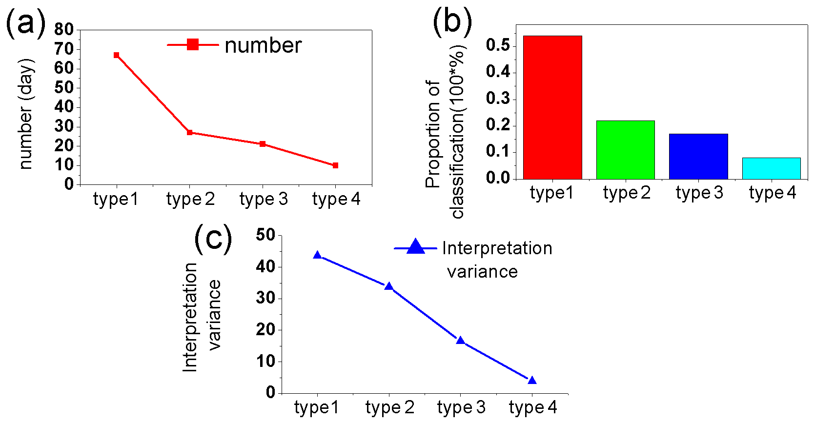
Figure 2 The four pollution weather types as a function of their (a) number of samples, (b) proportion with respect to the total number of samples, and (c) interpretation variance.

3 Results and discussion

3.1 Pollution weather type classification and horizontal characteristic analysis

In this study, the 925 hPa geopotential height was used to classify the pollution weather types into four categories with the REOF method, as shown in Fig. 1: (a) type 1, that is, influenced by southerly winds at the rear of the high-pressure system; (b) type 2, that is, influenced by easterly winds at the bottom of the high-pressure system; (c) type 3, that is, a weak downdraft effect in the high-pressure system; and (d) type 4: no significant weather system. In this study, we observed 125 d of heavy polluted weather. Among these days, type 1, type 2, type 3, and type 4 had 67, 27, 21, and 10 d, respectively (Fig. 2), where the four weather types accounted for 53.6 %, 21.6 %, 16.8 %, and 8.0 % of the total sampled weather event days, respectively. The total interpretation variance of the four types for all events was 97.8 %, while the independent interpretation variance was 43.69 %, 33.68 %, 16.51 %, and 3.92 %, respectively (Fig. 2). This indicates that an objective weather classification can effectively obtain the main feature information of the pollution weather types.

As shown in Fig. 1, the Beijing area is located toward the west of the high-pressure system that has its center located in the sea. The low-pressure system is located in the northern Hebei province for type 1, where southerly winds control the 925 hPa, which is favorable for the regional transportation of pollutants. Type 1 is similar to the results of pattern 2 and patter 4 by Zhang et al. (2016) accompanied by regional transmission characteristics. Type 1 is also similar to the results of type 1 by Miao et al. (2017), with southerly winds throughout the layer. When type 2 appears, the Beijing area is located at the bottom of the high-pressure system in Northeast or North China. In the plain area, the sea level pressure in the eastern part of Beijing is higher than that in the central Beijing area, such that there is an evident pressure gradient. Due to pressure-gradient forcing, the boundary layer appears within the easterly wind component while the easterly wind speed is smaller, which leads to pollutant convergence into the plains along the Taihang Mountains. When type 3 appears, the high-pressure center is located in the middle of Mongolia, where Beijing is in the front of the weak high-pressure system, with a northwest current at 925 hPa. However, the wind speed is lower than that affected by strong cold air, because of which it is difficult to penetrate the lower layer of the boundary layer and the wind can only exist in the upper atmosphere of the boundary layer. When type 4 appears, western Mongolia is a high-pressure region and southern Hebei province is a low-pressure area, where there is only a low-pressure system with a smaller spatial and temporal scale. The synoptic-scale low-pressure system is already located over the sea in the eastern Jianghuai region, showing that the high and low pressures corresponding to the synoptic-scale system are far from the Beijing area, which results in a weak synoptic-scale pressure gradient in Beijing and the surrounding areas (Fig. 1d). Most areas in North China do not have strong weather systems, and the average wind speed in the boundary layer is smaller, which is favorable to the formation and maintenance of the local circulation considering the topography in the Beijing area (Fig. 1i). The wind speed of type 4 in the lower boundary layer is more difficult to regulate via the evolution of the wind field based on the effect of descending momentum. Therefore, the dynamic pollutant process in the boundary layer in type 4 is more related to the local circulation.

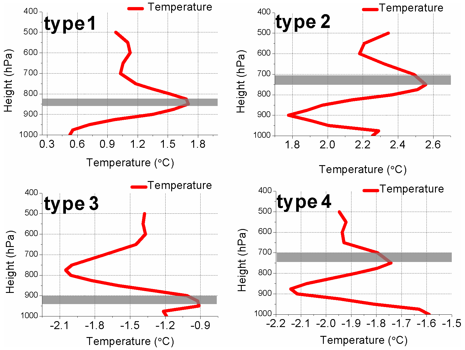
Figure 3 Vertical distribution of temperature in the pollution boundary layer of four types in the Beijing area. Solid red lines represent temperatures at different heights. Gray shade represents the top of the inversion layer.

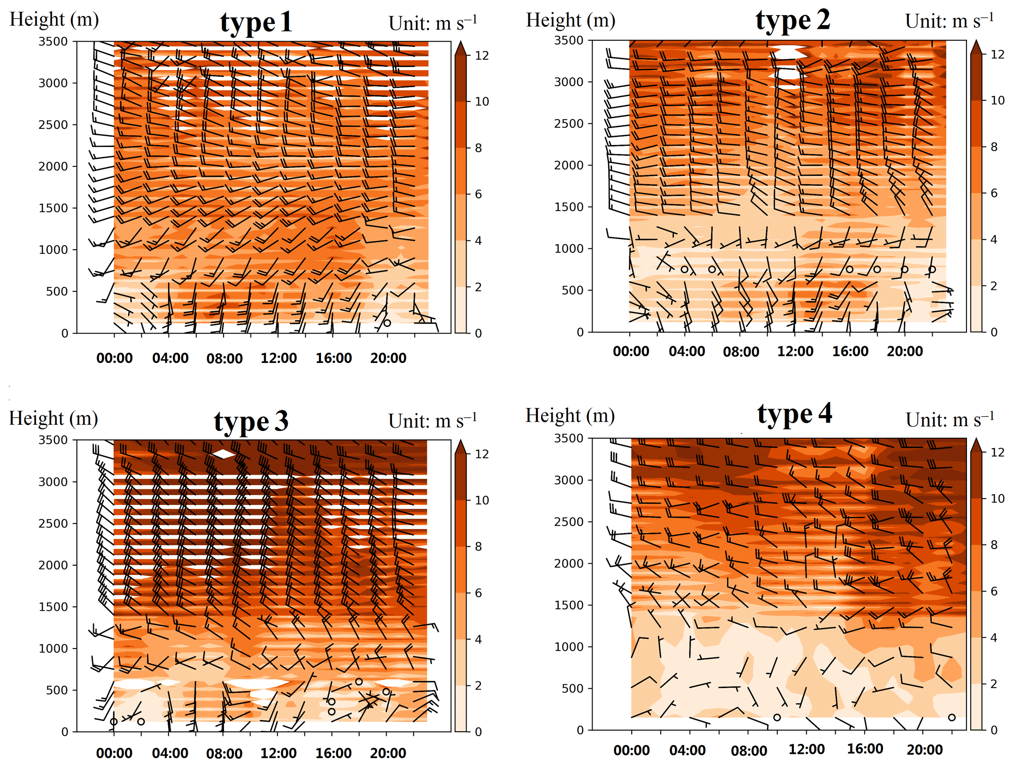
Figure 4 The mean wind field characteristics of the four pollution weather types in the Beijing observatory (39.93^∘ N, 116.28^∘ E) (varying colors, based on the color bar to the right of each panel, represent the wind speed in m s⁻¹; the x axis is in Beijing time from 00:00 to 23:00 CST; the y axis is the height in m).

Figure 5 The vertical speed profiles in the four pollution weather types (type 1: red, type 2: blue, type 3: green, and type 4: red) in the Beijing observatory (39.93^∘ N, 116.28^∘ E). The negative values represent ascending motion while positive values represent descending motion under the pressure coordinate (unit: Pa s⁻¹).

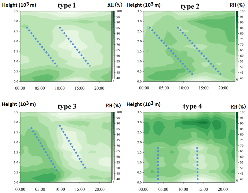
Figure 6 Average characteristics of the relative humidity (RH) field in the boundary layer under four pollution types in the Beijing observatory (39.93^∘ N, 116.28^∘ E) (shadow represents relative humidity, unit: %; x axis is Beijing time from 00:00 to 23:00 CST; y axis is height, unit: km).

3.2 Vertical thermal and dynamic structure characteristics under four weather types

The vertical structure of the atmosphere is very important for the formation and evolution of extreme haze events. The vertical thermal and dynamic structures of four weather types are investigated in three-dimensional view. Figures 3 to 6 presented the vertical distribution of temperature, wind, and RH, respectively. The temperature in Fig. 3 and vertical speed profiles in Fig. 5 are averaged for each weather type by using the 6 h ERA-Interim reanalysis data, respectively. The hourly mean wind profiles in Fig. 4 are observed at the Beijing observatory, and the hourly mean relative humidity in Fig. 6 is measured with a microwave radiometer at the same site. According to the classification of weather type, the spatiotemporal average analysis of the observed data is carried out. To classify the pollutant regimes according to the various meteorological features, we summarized relevant thermodynamic and dynamic parameters in Table S1.

Figure 3 shows that the strong inversion is located at 800–900 hPa for type 1. In type 2, easterly winds with low temperatures influence the temperatures below 800 hPa, where a cooling layer appears at 900 hPa, with the height of inversion between 700 and 800 hPa. The inversion height for type 3 is the lowest among the four types due to the sinking motion, where the inversion is mainly below 900 hPa, which causes a rapid decline in the atmospheric capacity. The atmospheric structure is also relatively stable in type 4, whose inversion structure is similar to type 2. However, the inversion intensity (0.4 ^∘C) in type 4 is weaker than that in type 2 (0.7 ^∘C), and the wind speed is also small in type 4.

As shown in Fig. 4, the basic flow is the southerly wind below 2000 m in type 1, where a southwest wind appears from 500–2000 m. The south wind is below 500 m between 04:00 and 20:00 CST, and the easterly wind appears at other times. The south wind speed below 500 m is 4–6 m s⁻¹, which is higher than the easterly wind (2–4 m s⁻¹). In type 2, the basic flow above 1000 m is westerly wind, where the layer between 500 and 1000 m is a weak wind layer. We note that the wind velocity in this layer is the smallest when there is an increase in the easterly component below 500 m. This indicates that the weak wind layer is the wind shear transition layer between the westerly wind above 500 m and the easterly wind below 500 m. The easterly and westerly winds cancel each other out at this height and form a small wind velocity layer. From 04:00 to 20:00 CST, southerly winds appear below 500 m while we observe the appearance of easterly winds at other times. The space–time structure of the wind field below 500 m was similar to that of type 1, but the southerly wind speed was lower than in case of type 1. In type 3, the wind above 500 m originates from the northwest from 04:00 to 14:00 CST. At altitudes below 500 m, the wind is southerly during these hours and northerly at other times. Whether it is southerly or northerly, the wind speed is smaller. Mountain–plain wind in the Beijing area causes this diurnal and nocturnal circulation of the wind field. In type 3, the wind velocity below 500 m is less than that of type 1 and type 2 because the basic flow is northerly, where northerly wind is superposed onto the plain wind (southerly), which may weaken the southerly wind speed. The observed data are the superposition results of two-scale wind fields (i.e., local circulation and synoptic airflow). Westerly or weak northerly winds above 1000 m in type 4 control the atmosphere, where the wind velocity below 1000 m is significantly weak. For the majority of the time, the wind velocity is less than 4 m s⁻¹, but the mountain–plain diurnal cycle wind can still be observed from the diurnal variation in the wind direction. From 08:00 to 18:00 CST, the wind is southerly while mainly northerly at night. Weak wind speeds last for a long period in the boundary layer of type 4, because of which the local thermal and dynamic conditions can become the main factors that affect the spatiotemporal distribution of haze pollutants in Beijing.

Figure 5 shows that, above 700 hPa, type 1, type 2, and type 4 are ascending movements. The maximum of the synoptic-scale ascending movement appears in 900–950 hPa. With an increase in height, the intensity of the ascending movement gradually weakens, whereas in type 3, below 750 hPa can be characterized as a sinking movement. The intensity of the sinking movement increases gradually with decreasing pressure, where the maximum of the sinking movement appears at 900–950 hPa. The intensity of the subsidence movement from this layer at 900–950 hPa to the ground decreases a second time. Therefore, the sinking movement affects the inversion layer of type 3, where the height of the inversion layer is the lowest of all types, resulting in type 3 characterized by the smallest atmospheric capacity among the four types.

Based on Fig. 6, the relative humidity profiles for the four weather types have both similarities and differences in their space–time structures. The similarities in the four types are the increased and decreased relative humidity below 1000 m during the night and day, respectively, with a reverse in the relative humidity appearing at an altitude about 500 m during the day. The relative humidity of the surface layer decreases daily from 10:00 to 20:00 CST with an increase in the solar radiation. The thickness of the dry layer in the surface layer increases continuously, reaching its maximum height at ca. 14:00 or 15:00 CST every day, but the maximum height of the dry layer does not exceed 500 m. The top of the dry layer is the reverse of the relative humidity layer. Above 1000 m, the relative humidity of the other three types, except type 2, decreases significantly during the day. However, the relative humidity increased evidently in type 4 above 2000 m. As mentioned in Sect. 3.1, in type 4, Beijing is located between a high pressure and a low pressure and in the front of the weak frontal zone. Stratus clouds with high stability are located in the front of the weak frontal zone above 2000 m, so relative humidity above 2000 m is higher.

The difference in the relative humidity field among the four types can be summarized as follows. The average relative humidity below 1000 m is higher than that above 1000 m. The inverse relative humidity structure appears below 500 m in type 2 and type 3 from 00:00 to 05:00 CST, with a maximum relative humidity center of more than 90 %. Above 500 m, the relative humidity also increases from 05:00 to 12:00 CST. The relative humidity structures of type 1, type 2, and type 3 all contain a baroclinic structure from lower to higher levels, where the baroclinic structure in type 2 is more evident because the basic flow in type 2 is westerly, which reflects the baroclinic characteristics of the atmosphere in the mid–high latitudes of East Asia. The basic flow is generally westerly in this area, where type 1 and type 3 are more typical of the disturbances in the northerly and southerly wind in the westerlies, which is the fluctuation feature of the basic flow (Fig. 6). The relative humidity profile in the pollution boundary layer formed under the condition of wave–current interaction in the atmosphere.

Type 2 has strong westerly characteristics below 3000 m (Fig. 4), which reflects more baroclinic characteristics in the atmospheric vertical structure for the westerlies. Based on the analysis of the wind field, type 4 is characterized by an average wind speed that is the weakest among the four types. Three important factors determine the baroclinicity, that is, the density gradient, the pressure gradient, and the intersection angle between the density surface and pressure surface. This may be an important factor for why the relative humidity field has more barotropic characteristics. From the analysis of the baroclinic and barotropic characteristics, we can observe that the weather systems of type 1, type 2, and type 3 have a significant influence on the accumulation and transport of pollutants in the Beijing area. The mountain–plain wind in type 4 can occur due to weakening in the weather system (Fig. 4).

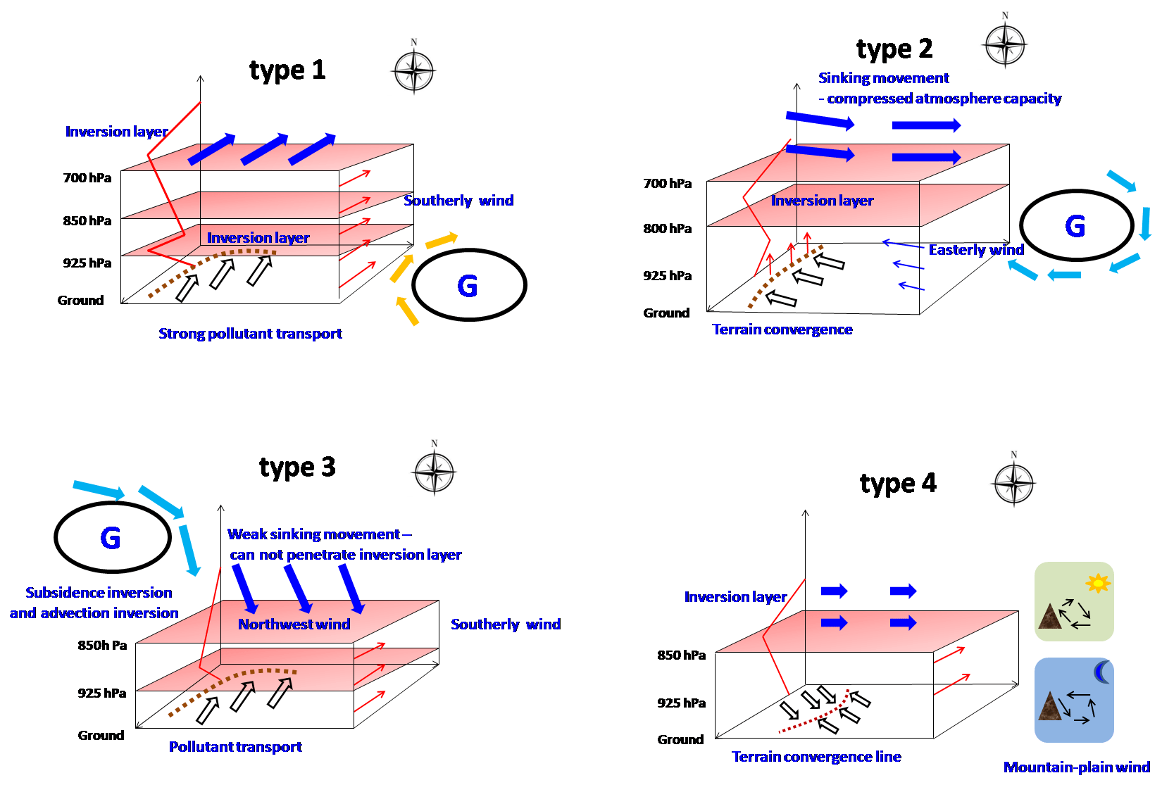
Figure 7 A thermodynamic and dynamic structure conceptual model of the pollution boundary layer for the four types of weather in the Beijing area. Arrows represent wind directions at different heights. Hollow arrows represent the ground horizontal wind field, thin red and blue arrows represent wind fields at different heights, and thick blue arrow represents the upper wind field. The dark red dots represent ground convergence lines, including (1) convergence between wind fields and (2) convergence between wind fields and topography. The solid red line is temperature. The Beijing area is located within the lowest rectangle, and the small figure in type 4 represents mountain–plain winds with a daily cycle.

3.3 Construction of 3D conceptual model for the pollution boundary layer

Based on the characteristics of the circulation field and the vertical thermodynamic structure for the four weather types, we established conceptual models of the boundary layer structure under the influence of the four pollution weather types. Because the vertical axes are different for the wind profile and temperature profile, we chose the pressure axis, which is widely used in meteorology, to make conceptual model. In the Beijing area, 700, 850, and 925 hPa layers are generally located at a height of about 3000, 1500, and 800 m, The four types are as follows: (a) type 1 – southerly transport, (b) type 2 – easterly convergence, (c) type 3 – sinking compression, and (d) type 4 – local accumulation (Fig. 7). When type 1 appears, the Beijing area is located at the rear of the high-pressure system, consistent with southerly winds throughout the atmosphere (Figs. 1e and 4), and multilayer inversion occurs in the boundary layer (Fig. 3). Under the influence of a southerly wind, haze pollutants accumulate in front of the Yan and Taihang Mountains. The air pollutants in the Hebei region have evident regional transport features (Fig. 1). When type 2 appears, the Beijing area is located at the bottom of the high-pressure system, where the air above 850 hPa (about 1500 m in Beijing) is a westerly wind, with easterly winds below 850 hPa. Under the influence of easterly winds below 850 hPa, haze pollutants tend to accumulate in front of the Taihang Mountains. The cross-mountain air mass flows from west to east, preventing the further dispersion of air pollutants in front of the Taihang Mountains. When type 3 appears, a weak high-pressure system controls the Beijing area. A weak subsidence northwest flow influences the atmosphere above 850 hPa, which further compresses the capacity of the atmosphere to absorb pollutants in the boundary layer. The southerly wind at 850 hPa is favorable for pollutant transportation in the region and accumulation in front of the Yan and Taihang Mountains. The atmospheric vertical structure in the high-level northwest wind and low-level southward wind provides excellent conditions for the stability of atmospheric stratification with respect to dynamic conditions and a thermal structure. The 850 hPa southerly winds favor regional pollutant transport and their accumulation in the area along the Yan and Taihang Mountains. The atmospheric vertical structure of the high-level northwest wind and low-level southerly wind provides excellent conditions for stratification stability in terms of dynamic–thermal structures because southerly wind at 850 hPa is warm advection, where advection inversion can form in the boundary layer, while weak subsidence above 850 hPa can cause subsidence inversion. These two inversion mechanisms are coupled at the interface between the northwest wind and southerly wind, resulting in stable atmospheric stratification. When type 4 appears, there is often no evident synoptic-scale system surrounding Beijing, with a weak pressure gradient above 850 hPa. Therefore, the average wind speed is weak. The most important local circulation in Beijing, that is, the mountain–plain wind, begins to form in the boundary layer and plays an important role in the spatial and temporal distribution of atmospheric pollutants, with the wind direction continuously shifting from the south to the north. The air pollutants accumulate near the terrain convergence line formed by the mountain–plain wind. The terrain convergence line also swings from north to south, such that air pollution in the Beijing area often appears as a “different sky” relative to a clean sky in the north and a polluted sky in the south.

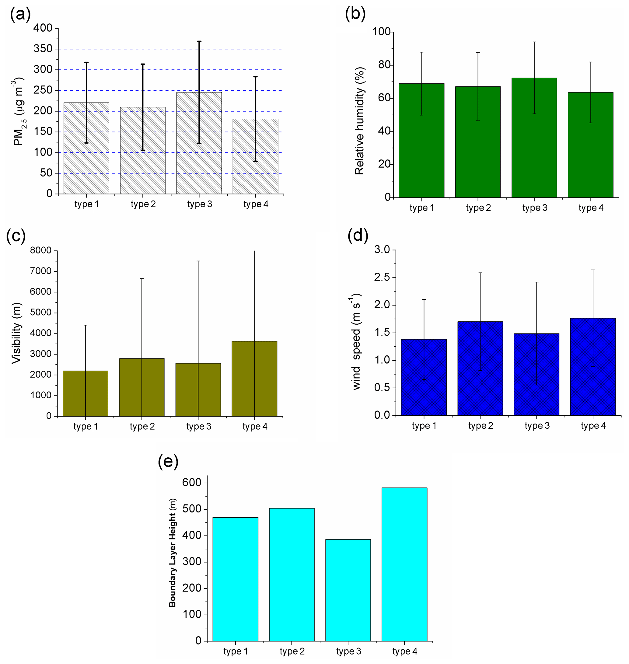
Figure 8 The four pollution weather types in the Beijing area: (a) average daily PM_2.5 concentration at 12 state-controlled stations (unit: µg m⁻³), (b) average daily relative humidity at the Beijing observatory (unit: %), (c) average daily visibility at the Beijing observatory (unit: m), (d) average daily wind speed at the Beijing observatory (m s⁻¹), and (e) the boundary layer height from the tower station at the Institute of Atmospheric Physics, Chinese Academy of Sciences (unit: m).

3.4 Effects of the four pollution weather types

3.4.1 Statistical analysis: effects of the four weather types on haze pollution

Figure 8 shows the statistical characteristics of the PM_2.5 concentrations and meteorological elements in terms of the four polluted weather types. The daily average PM_2.5 concentration in type 3 is the highest at 245 µg m⁻³, and type 4 is the lowest at 181 µg m⁻³ (Fig. 4). The daily average relative humidity values of the four pollution weather types are >60 %, with a maximum relative humidity of 72.3 % in type 3 and a minimum relative humidity of 63.5 % in type 4 (Fig. 8b). Under the influence of a high relative humidity and high PM_2.5 concentration, the daily average visibility for the four heavy pollution weather types is less than 4000 m, with a minimum daily average visibility of 2193 m in type 1. The maximum daily average visibility is 3624 m in type 4 (Fig. 8c). The mean 24 h wind speeds for the four pollution weather types are all less than 2.0 m s⁻¹.

The mean daily wind speeds of type 1 and type 3 are both smaller, that is, 1.38 and 1.49 m s⁻¹, respectively. The mean daily wind speeds of type 2 and type 4 are relatively higher, that is, 1.70 and 1.76 m s⁻¹, respectively (Fig. 8d). There is a significant negative correlation between the boundary layer height and PM_2.5 concentration. The lowest boundary layer height was 386.5 m for type 3, followed by type 1, whereas type 4 had the highest boundary layer height.

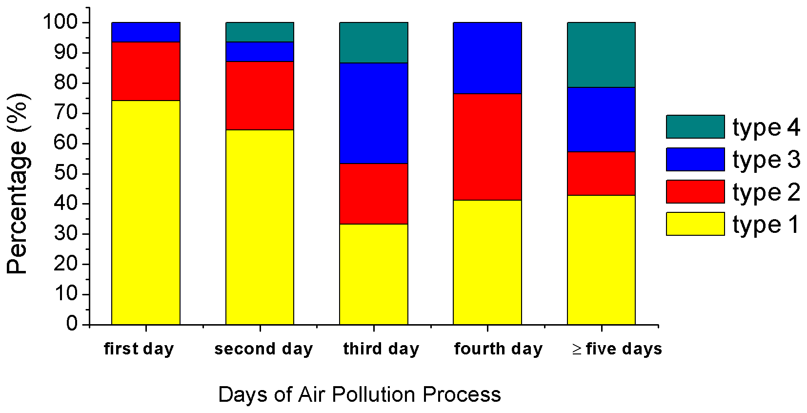
Figure 9 Time distribution of the four pollution weather types (yellow, red, blue, and green represent type 1, type 2, type 3, and type 4, respectively) during pollution events in the Beijing area.

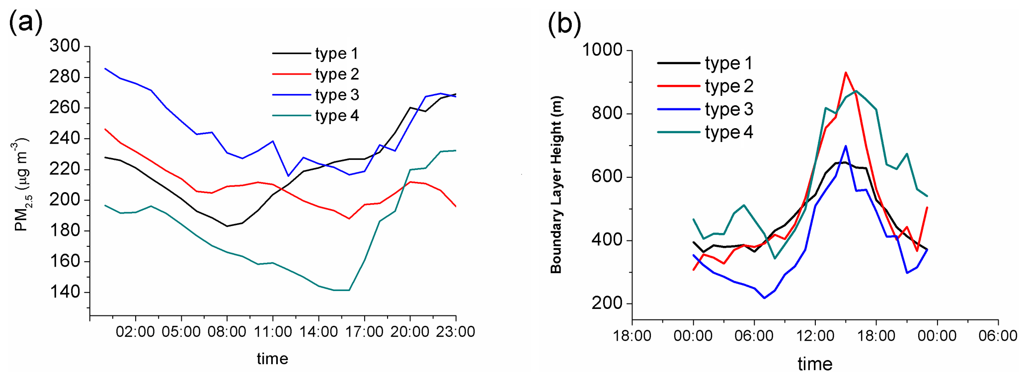
Figure 10 Diurnal variation characteristics of the (a) PM_2.5 averaged concentration (µg m⁻³) and (b) boundary layer height (m) under the four pollution weather types in the Beijing area (39.974^∘ N, 116.372^∘ E,) (x axis: 00:00–23:00 CST).

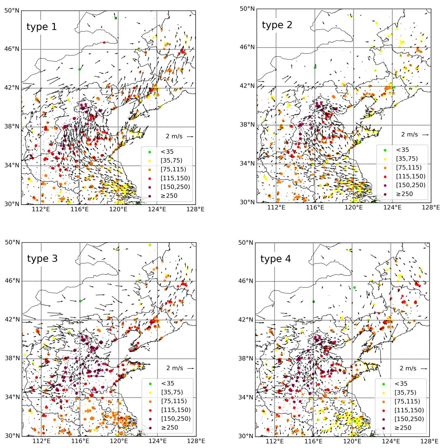
Figure 11 Spatial distribution of the PM_2.5 concentration (unit: µg m⁻³) and wind field near the ground.

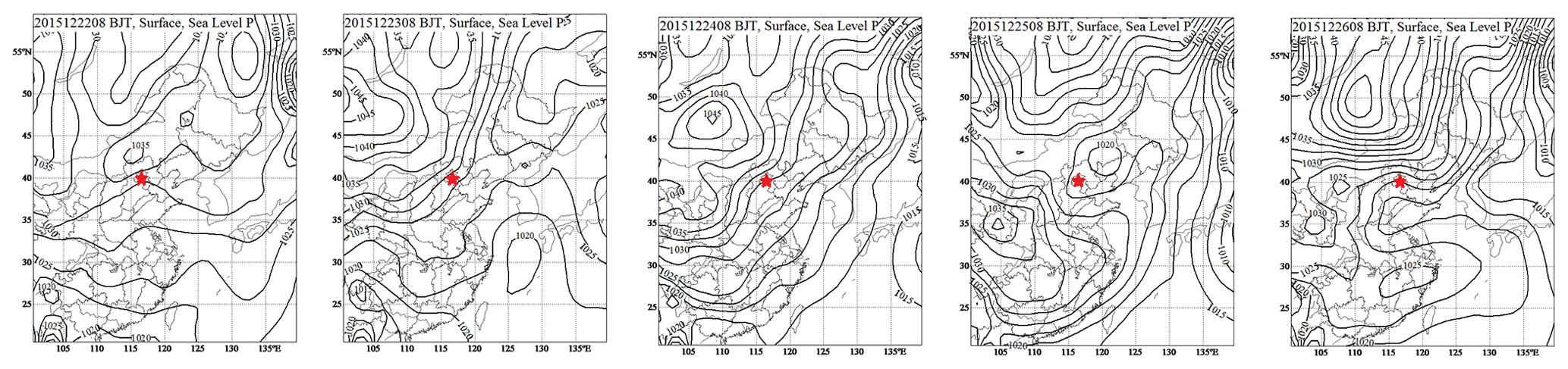
Figure 12 Sea level pressure (hPa) at 08:00 CST from 22 to 26 December 2015 (the red five-pointed star represents the Beijing area).

In this study, we calculated the distribution of the weather types from the first to last day of the persistent haze pollution events (Fig. 9). The daily synoptic types from the first to eighth day of persistent haze pollution events were calculated. As the number of pollution events that lasted more than 5 d is relatively small, the classification results were combined with the statistics for the events defined as greater than or equal to 5 d. The results show that the cumulative proportion of type 1 and type 2 occurrences on the first and second pollution day are more than 80 %, indicating that regional transport plays a more prominent role in the initial stage of haze pollution formation, which is consistent with previous analyses (Zhong et al., 2018). On the third day and thereafter, the proportion of type 1 began to decrease but still exceeded 30 %. Type 2, type 3, and type 4 began to alternately affect the Beijing area. This indicates that, after the first and second days, the center of high pressure over East China in type 1 began to move eastward away from the mainland. Beijing is located at the rear of the high-pressure system, where the PM_2.5 concentration corresponding to type 1 increases throughout most of the day. The timing of the initial rise in the PM_2.5 concentration is the earliest among the four types (Fig. 10a), which indicates the role of the rear within the high-pressure system in the transmission of pollutants (Fig. 11). When the upstream weather system begins to affect the Beijing area, it is occasionally located at the bottom of the high-pressure system (type 2). The diurnal variation in the PM_2.5 concentration in type 2 was similar to the mean annual variation in the PM_2.5 concentration in the Beijing area. The first peak was at 10:00 and the second was at 20:00 (Zhao et al., 2009) (Fig. 10a). Easterly or southeasterly winds appear near the ground and the concentration of PM_2.5 in Tianjin drops (Fig. 11). The weak high-pressure system in type 3 can directly affect the haze pollution diffusion conditions in the Beijing area, but the intensity of the cold air behind the upper trough is weak. The PM_2.5 concentration in type 3 is higher at night and lower during the day, with the highest average PM_2.5 concentration among the four types. Based on this analysis, we can observe that, in type 3, the height of the inversion layer is the lowest and the atmospheric capacity to contain pollutants is also the lowest under the influence of a weak downdraft (Fig. 10a). This has resulted in very small wind speed near the ground and large areas of air pollution in the north of China (Fig. 11). In type 4, there is no evident weather system that affects the Beijing area. An increase in the thermal difference between the mountain and plain affects local circulation development. A shear line of the wind field formed by local circulation can be seen in the North China Plain (Fig. 11). The average PM_2.5 concentration in type 4 is the lowest among the four types. The diurnal variation in the PM_2.5 concentration shows a typical “v” pattern. After sunrise, the PM_2.5 concentration begins to decrease, while, after sunset, the PM_2.5 concentration increases significantly, which was due to the fluctuation of aerosols under local meteorological conditions (Fig. 10a). Based on Fig. 10b, the boundary layer height of type 3 is the lowest among all types for the major part of a day, which is mainly related to the suppression of the weak synoptic-scale downdraft. The change in the trend of the boundary layer height is similar between type 2 and type 4 for most of the day. However, the boundary layer height is less developed when the thermal conditions are strongest between 12:00 and 18:00 CST, which is similar to type 3. The boundary layer heights of type 2 and type 4 are relatively high, and the corresponding PM_2.5 concentrations are the lowest out of the four pollution types (Fig. 10b).

The above analysis shows that in one persistent multi-day pollution event the weather patterns that affect the Beijing area change daily; that is, they also change according to the basic principles of synoptic dynamics, which is the natural development and evolution of Rossby waves in the mid–high-latitude westerly belt. This also indicates that it is not appropriate to classify a multi-day pollution event as a defined type (such as the low-pressure or high-pressure type). We can not rule out the possibility that a pollution event may occur for several consecutive days under the influence of a low-pressure system, which is a rare event. Even then, this may also be a combination of different low-pressure systems. In addition, we note that, in one persistent multi-day heavy pollution event, different types of pollution weather types are linked together in a permutation that affects the structure of the boundary layer and thus the change in the PM_2.5 concentration (Fig. 9). As different types of weather systems form different haze pollution events, we discuss the type of boundary layer structure formed by certain weather systems in the Beijing area and how this boundary layer structure influences the evolution of haze pollution formation in the next section.

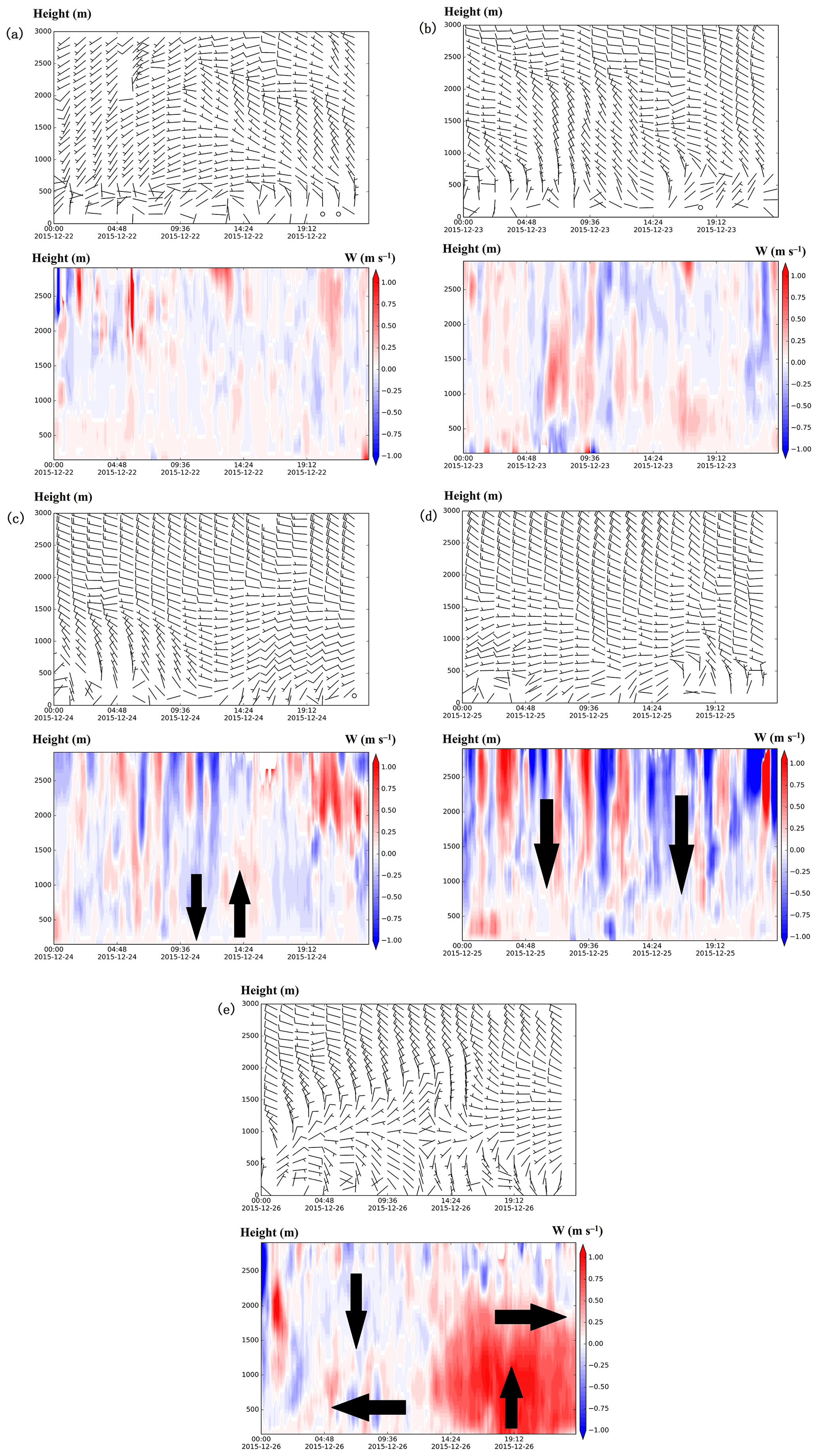
Figure 13 The horizontal and vertical wind field characteristics in the Beijing observatory (39.93^∘ N, 116.28^∘ E) from 22 to 26 December 2015 (a–e, above is the horizontal wind field, below is the vertical wind speed (W), wind speed is in m s⁻¹, and the red shadow represents the upward movement; blue represents the sinking movement; the x axis is in Beijing time; the y axis is the height in meters).

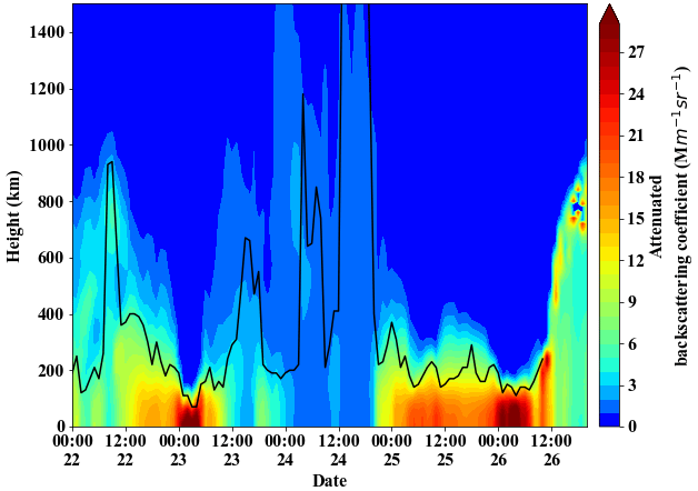
Figure 14 Aerosol backscattering intensity (${\mathrm{Mm}}^{-\mathrm{1}}{\mathrm{sr}}^{-\mathrm{1}}$) from 22 to 26 December 2015 in the Beijing area (39.974^∘ N, 116.372^∘ E) (they axis is the height in meters and the x axis is in Beijing time).

Figure 15 Vertical temperature profile of Beijing from 22 to 26 December 2015 in the Beijing observatory (39.93^∘ N, 116.28^∘ E) (unit: ^∘C).

3.4.2 Effects of four weather types on the 3D spatiotemporal evolution of haze pollution

An example of a 5 d haze process (22 to 26 December 2015) is adopted to investigate the effects of four weather types including the boundary layer structure on the three-dimensional structure of the haze pollution process. The day of 22 December is type 1, the whole layer is southerly wind (Fig. 13), and the ground is the convergence zone (Fig. 12), which facilitates regional pollutant transport (Fig. 14). The vertical wind speed is weak upward movement (Fig. 13), and the temperature inversion is maintained throughout the day (Fig. 15), which is favorable for the accumulation of pollutants. Under the influence of southerly winds, the sensitive source areas related to the Beijing area are generally the plain areas along the Taihang Mountains in Hebei province (Wang et al., 2018). According to the dynamics, the positive vorticity advection in the direction of Beijing forms in the plain area. The positive vorticity advection in this boundary layer has two functions. First, the positive vorticity airflow is affected by the friction, coriolis effect, and pressure-gradient force. Second, the positive vorticity advection continuously transports the converging space field to the Beijing area and, at the same time, also transfers a large amount of external pollutants.

Type 3 is on 23 December. The ground is controlled by high pressure (Fig. 12), the atmosphere is prevailing northwest wind below 3000 m (Fig. 13), and the boundary layer height further decreases (Fig. 15). There are few relevant studies on type 3. Normally, northerly winds originate from regions with low emissions, which carry clean air to Beijing and the surrounding area and dilute pollutants, but the northerly winds should reach the surface. In some cases, the northerly winds only occur above the boundary layer, which causes the subsidence motion and further results in local pollutant accumulation. We found that the research results of Wu et al. (2017) put emphasis on the importance of subsidence motion on the haze formation mechanism in the conceptual model, which is consistent with the key role of weak subsidence motion in type 3. The thickness of the haze layer formed by regional transmission and local accumulation is less than 300 m (Fig. 14).

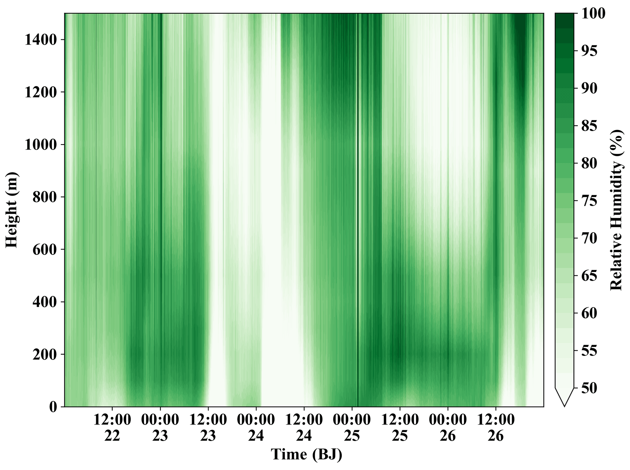
Figure 16 Vertical relative humidity profile of Beijing at 08:00 and 20:00 CST from 22 to 26 December 2015 in the Beijing observatory (39.93^∘ N, 116.28^∘ E) (unit: %).

Type 4 is on 24 December, and the ground is the convergence zone (Fig. 12). The aerosol concentration and relative humidity in the Beijing area drops rapidly and then rises rapidly, and the boundary layer rises to more than 1500 m during the period when the aerosol concentration drops (Figs. 14 and 16). Under the interaction of the weak synoptic system and local circulation, the pollution zone swings in adjacent areas along the mountains. Some studies have revealed that the effects of local circulation on pollutants are mainly caused by local mountain–plain breeze circulation and sea–land breeze circulation (Li et al., 2018, 2020). These studies require observations with high spatial and temporal resolution to identify boundary layer structures.

Type 3 occurs on 25 December once again when the northwest wind appears again in the upper atmosphere, the vertical movement is a continuous weak sinking movement (Fig. 13), and the boundary layer height continues to maintain below 300 m (Fig. 14). The temperature inversion is maintained throughout the day (Fig. 15). The day of 26 December is type 2. The Beijing area is located at the bottom of the high-pressure system (Fig. 12), and easterly winds prevail in the lower layer of the boundary layer (Fig. 13). The diffusion conditions of air pollution here can be divided into two stages. In the first stage, the easterly wind is below 1000 m, and the northerly wind is above 1000 m, so the aerosol can not spread to the upper atmosphere (Fig. 13). In the second stage, the high pressure continued to move eastward and lost its influence on the Beijing area. When the northerly wind over 1000 m changed to the westerly or southwesterly wind, the upper and lower atmosphere were connected, and the upward movement of m s⁻¹ magnitude was stimulated in the boundary layer (Fig. 13); the haze process ends when the aerosol is lifted into the upper atmosphere (Fig. 14).

4 Conclusions

In this study, we objectively classified pollution weather events based on the REOF method using integrated observation data from meteorology and the environment, combined with the ERA-Interim reanalysis data (0.125^∘ × 0.125^∘). We then synthesized the thermodynamic and dynamic structures of the boundary layer under the different pollution weather types to construct the corresponding boundary layer conceptual models. The results show that four weather types mainly affect the pollution events in Beijing: (a) type 1 – southerly transport, (b) type 2 – easterly convergence, (c) type 3 – sinking compression, and (d) type 4 – local accumulation. The explained variance in the four pollution weather types were 43.69 % (type 1), 33.68 % (type 2), 16.51 % (type 3), and 3.92 % (type 4), respectively.

In persistent pollution events, the proportion of type 1 and type 2 occurrences was more than 80 % on the first and second days, with subsequent alternations to the other types. The atmospheric structures of type 1, type 2, and type 3 have typical baroclinic characteristics in the mid–high latitudes, indicating that synoptic-scale systems, together with local circulation, affect the accumulation and transport of pollutants in the boundary layer. On the other hand, the atmospheric structures of type 4 have typical barotropic characteristics, which indicates that local circulation plays a major role in pollutant accumulation and transport. This is the first time that the baroclinic and barotropic characteristics of the atmosphere have been introduced into the discussion of pollution boundary layer.

Among the four types, southerly winds, with certain thicknesses and intensities, appeared in the boundary layer of type 1, which was favorable for the transportation of pollutants to Beijing, accumulating more in areas along the Yan and Taihang Mountains. On the other hand, the pollution level in the central plain area of Hebei was relatively small. For type 2, the pollutants mainly concentrated along the Taihang Mountains due to the influence of the interaction between weak easterly winds and topography. The vertical structure of the atmosphere was unfavorable for pollutants to ascend into the mountains. Type 3 had the lowest inversion height and boundary layer height and the highest surface relative surface humidity, which are favorable for PM_2.5 hygroscopic growth. Correspondingly, type 3 had the highest PM_2.5 concentration. Type 4 had the highest boundary layer height and lowest surface relative humidity among the four pollution types, whose PM_2.5 concentration was relatively low when exposed to local mountain–plain winds. Pollutant accumulation is related to dynamic oscillation along the convergence line of the mountain terrain. The results of this study allow us to understand the formation mechanism of different heavy pollution boundary layers from synoptic-scale and boundary layer perspectives, as well as to provide scientific support for scientific emission reduction and air quality prediction. The different heavy pollution weather types and heavy pollution boundary layers not only reflect the interaction between the atmospheric mean flow and fluctuation, but also reflect the process of heavy pollution weather types shaping the boundary layer. In addition, through the analysis of the 1–4 types of pollution processes (22 to 26 December 2015), we further illustrate the influence of different weather systems on the shaping of the pollution boundary layer in the continuous pollution process.

Although we attempted to collect data on all types of atmospheric pollution boundary layer structures in the Beijing area, there are still certain data samples that were not collected. These data can also explain the pollution characteristics associated with the four heavy pollution boundary layers from other factors, such as PM_2.5 composition data. We also speculate that there is feedback between aerosols and the boundary layer, which was not examined in this study. Although there have been numerous studies on atmospheric pollutant transport, there are few studies on 3D pollutant transportation, which will be the focus of our future investigations.