Modeling the impact of COVID-19 on air quality in southern California: implications for future control policies

In response to the coronavirus disease of 2019 (COVID-19), California issued statewide stay-at-home orders, bringing about abrupt and dramatic reductions in air pollutant emissions. This crisis offers us an unprecedented opportunity to evaluate the effectiveness of emission reductions in terms of air quality. Here we use the Weather Research and Forecasting model with Chemistry (WRF-Chem) in combination with surface observations to study the impact of the COVID-19 lockdown measures on air quality in southern California. Based on activity level statistics and satellite observations, we estimate the sectoral emission changes during the lockdown. Due to the reduced emissions, the population-weighted concentrations of fine particulate matter (PM_2.5) decrease by 15 % in southern California. The emission reductions contribute 68 % of the PM_2.5 concentration decrease before and after the lockdown, while meteorology variations contribute the remaining 32 %. Among all chemical compositions, the PM_2.5 concentration decrease due to emission reductions is dominated by nitrate and primary components. For O₃ concentrations, the emission reductions cause a decrease in rural areas but an increase in urban areas; the increase can be offset by a 70 % emission reduction in anthropogenic volatile organic compounds (VOCs). These findings suggest that a strengthened control on primary PM_2.5 emissions and a well-balanced control on nitrogen oxides and VOC emissions are needed to effectively and sustainably alleviate PM_2.5 and O₃ pollution in southern California.

1 Introduction

Anthropogenic emissions from various emission sources, including transportation, industrial, agricultural, residential, and commercial sectors, contribute to California's long-existing air pollution problems (e.g., Shirmohammadi et al., 2016; Hong et al., 2015; Warneke et al., 2013). The major pollutants include, but are not limited to, fine particulate matter (PM_2.5), nitrogen dioxide (NO₂), sulfur dioxide (SO₂), and ozone (O₃). Exposure to these pollutants has been correlated with an increased rate of morbidity and mortality (Wang et al., 2019). Mitigating the adverse effects of air pollution by reducing air pollutant emissions from major sectors has been and will continue to be a major public policy challenge. However, the effect of emission reductions from various sources on air quality improvement is subject to substantial uncertainties because such effects cannot be directly measured and because the atmospheric chemistry processes are highly nonlinear and complicated (Zhao et al., 2019b, 2015; Chen et al., 2013). The recent coronavirus disease of 2019 (COVID-19) provides an unprecedented opportunity for a more robust understanding of the environmental impacts brought by the emission reductions.

More than 200 countries and territories around the world have reported a total of about 53 million confirmed cases of COVID-19 that originated from Wuhan, China, and a death toll of more than 1 300 000 (World Health Organization, 2020). California is one of the most affected states in the United States (US), partly because its poor air quality makes Californians more susceptible to infectious diseases such as COVID-19 (Bashir et al., 2020; Copat et al., 2020). In response to the emergence of COVID-19, statewide stay-at-home orders and related actions (e.g., closure of nonessential businesses) took effect on 19 March 2020 in California. These orders are expected to reduce vehicle traffic and industrial activities, thereby changing the air pollutant emissions and air quality in the state. It is essential to obtain a high-spatiotemporal-resolution estimation of air pollution for a better understanding of the atmospheric impacts caused by changes in anthropogenic activity associated with the COVID-19 pandemic.

A number of studies emerged soon after the start of the COVID-19 pandemic and the subsequent lockdown to assess the impact of the pandemic on air quality over various regions around the world. For example, Archer et al. (2020) compared the observed concentrations at all available ground monitoring sites in the US between April 2020 and the prior 5 years (2015–2019) and found statistically significant decreases in NO₂ concentrations at more than 65 % of the monitoring sites, with an average drop of 2 ppb. Pan et al. (2020) compared the surface air quality monitoring data in California during the period 20 March–5 May 2020 with those in 2015–2019 and found that PM_2.5 in 2020 exhibited a notable decrease, which could result from emission reductions associated with the COVID-19 lockdown. Similar findings, i.e., reduced PM_2.5 and NO₂ concentrations, are also reported for China (e.g., Chu et al., 2021; Le et al., 2020; Liu et al., 2020; Marlier et al., 2020; Shi and Brasseur, 2020; Miyazaki et al., 2020b), India (e.g., Pathakoti et al., 2020; Sharma et al., 2020), and Europe (e.g., Chen et al., 2020; Menut et al., 2020; Sicard et al., 2020; Ordóñez et al., 2020) based on surface and/or satellite observations. For O₃, the concentrations either increased or slightly decreased during the pandemic, depending on the region (Bekbulat et al., 2020; Huang et al., 2021; Pan et al., 2020; Zhao et al., 2020). Most of the above studies, however, are limited to comparing observations with and without lockdown measures, which correspond to different time periods under different meteorological conditions.

Meteorology plays significant roles in air pollution formation, transport, deposition, and transformation (P. Wang et al., 2020), which is a very important factor that affects concentrations of O₃ and PM_2.5 (Stewart et al., 2017). The changes in air quality due to meteorological variations may obscure the effects of emission changes during the COVID-19 lockdown. Using the Community Multiscale Air Quality model, P. Wang et al. (2020) showed that the benefits of emission reductions were overwhelmed by adverse meteorology over the North China Plain, and severe air pollution events were thus not avoided. Goldberg et al. (2020) reported that meteorological patterns were especially favorable for low NO₂ in much of the United States in spring 2020, complicating comparisons with spring 2019; meteorological variations between years can cause ∼ 15 % differences in monthly mean column NO₂. In view of this, a modeling approach is necessary to accurately assess the impact of lockdown measures by excluding the possible effects of meteorological conditions and to examine the possible mechanisms responsible for the changes in the air pollutant concentrations. In addition, while previous studies have evaluated air quality changes in different regions due to the emission reductions associated with the COVID-19 lockdown, it remains unclear how the COVID-19-induced emission reductions and the concurrent meteorological variations influence air quality in California.

The objective of this study is to investigate the air quality impact of the emission reductions in southern California in association with COVID-19 by employing high-resolution atmospheric modeling in combination with surface observations. Based on the statistics of activity levels together with constraints from satellite observations, we estimate the sectoral emission changes during the COVID-19 lockdown. We then conduct model simulations using the Weather Research and Forecasting model with Chemistry (WRF-Chem) for the periods before and during the COVID-19 lockdown to investigate the effects of reduced emissions and meteorology on air pollution, respectively. Understanding how air quality responds to the emission reductions during the COVID-19 pandemic will provide important insight into the future development and optimization of effective air pollution control strategies in southern California.

2 Method and data

2.1 Model configuration and emission estimation

We simulate the impact of COVID-19 lockdown measures on air quality using the WRF-Chem version 3.9.1, which considers highly nonlinear and complex meteorological and atmospheric chemistry processes. The simulation period is 18 February to 23 April 2020, which includes about 1 month before and after the California governor issued the stay-at-home (lockdown) order on 19 March (Pan et al., 2020). We apply the model to two nested domains: Domain 1 covers the western United States and its surrounding areas at a 12 km × 12 km horizontal resolution; Domain 2 covers California with a 4 km × 4 km resolution (Fig. 1). We focus our analysis on southern California (the red rectangle in Fig. 1), the largest metropolitan area in California, which is significantly affected by the lockdown measures. We classify model grids in southern California into urban and rural areas to facilitate the analysis of O₃ simulation results. To be classified as urban, an area in the US needs to have a population density of 1000 people per square mile (Ratcliffe et al., 2016), i.e., about 6000 people per 4 km × 4 km model grid. As we focus our analysis on southern California, one of the most densely populated areas in the US, we use a higher population density threshold of 30 000 people per model grid to better distinguish areas with different photochemistry regimes (Fig. S1 in the Supplement). We employ an extended Carbon Bond 2005 (CB05) (Yarwood et al., 2005) with chlorine chemistry (Sarwar et al., 2008) coupled with the Modal for Aerosol Dynamics in Europe volatility basis set (MADE VBS) (K. Wang et al., 2015; Ahmadov et al., 2012). MADE VBS uses a modal aerosol size representation and an advanced secondary organic aerosol (SOA) module based on the VBS approach. The aqueous-phase chemistry is based on the AQChem module used in the Community Multiscale Air Quality (CMAQ) model (K. Wang et al., 2015). The chemical initial and boundary conditions were extracted from the output of the Whole Atmosphere Community Climate Model (WACCM) (Marsh et al., 2013). A 6 d spin-up period is used to minimize the influence of initial conditions on simulation results. The vertical resolution, meteorological initial and boundary conditions, and physical options are the same as our previous modeling studies based on WRF-Chem for California (Zhao et al., 2019a; T. Y. Wang et al., 2020; Shi et al., 2019).

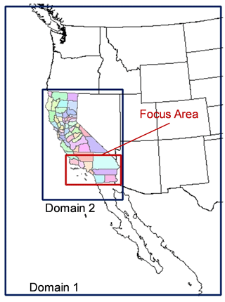
Figure 1 Simulation domains in this study. The red rectangle denotes the area of southern California where most analyses in this study are focused.

We obtain anthropogenic emissions in California without the influence of COVID-19 lockdown measures from the California Air Resources Board (CARB) for 2012, the latest year for which data are available (California Air Resources Board, 2018). We scale the 2012 emissions to 2020 levels by employing the relative changes for 2012–2018 in California from the National Emissions Inventory (NEI) trend report (US Environmental Protection Agency, 2018a) and assuming that the trends continued during 2018–2020. The anthropogenic emissions outside California are derived from the National Emission Inventory (US Environmental Protection Agency, 2018b) in 2011 and are scaled to 2020 following the same method. The biogenic, wind-blown dust, sea salt, and wildfire emissions are calculated online in WRF-Chem, as detailed in our previous studies (Zhao et al., 2019a; T. Y. Wang et al., 2020; Shi et al., 2019).

Table 1 Summary of model scenarios developed in this study.

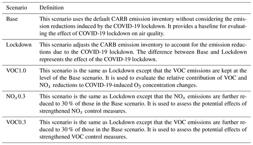
Table 2 The percentage of changes in air pollutant emissions during the COVID-19 lockdown relative to a hypothetical scenario without the lockdown in southern California.

In our baseline simulation (Base scenario in Table 1), we use the above emission inventories. To evaluate the effect of the COVID-19 response actions, we conduct another simulation (Lockdown scenario in Table 1) in which the CARB anthropogenic emission inventory after 19 March is adjusted to account for the emission changes due to the COVID-19 lockdown. Because of the lack of detailed emission data, which often take years to update, we rely on a number of key activity indicators to estimate the sector-specific relative changes in anthropogenic emissions (as summarized in Table 2), which are subsequently evaluated against satellite-derived emission estimates. For the transportation sector, we separately estimate the reduction rates for on-road, off-road, and aircraft emissions due to the COVID-19 lockdown. Specifically, we assume the reduction rates in gasoline and diesel vehicle emissions in the on-road sector to be the same as the reduction rates in gasoline and diesel production from the pre-lockdown period to the lockdown period, as documented by the California Energy Commission's Weekly Fuels Watch Reports (California Energy Commission, 2020b). We then estimate the reduction rates in total emissions from the on-road sector based on the relative fractions of gasoline and diesel vehicle emissions reported by the CARB emission inventory. Since the off-road sector involves few gasoline vehicles, we assume the reduction rates in off-road emissions to be the same as the reduction rate in diesel production. For the aircraft sector, we assume the reduction rates in aircraft emissions to be the same as the reduction rate in jet fuel production from the Weekly Fuels Watch Reports (California Energy Commission, 2020b). The changes in emissions from the industrial, residential, and commercial sectors are assumed to be proportional to the changes in electricity consumption by the corresponding sector, as summarized in the Energy Insights Reports of the California Energy Commission (California Energy Commission, 2020a). The changes in emissions from power plants are estimated as a function of the total electricity demand in California (California Energy Commission, 2020a). We also checked the emission change for power plants measured by the Continuous Emission Monitoring System (CEMS). There are certain differences between the emission reduction rates estimated based on the CEMS and electricity demand, but the difference only results in a less than 1 % difference in the total emissions of any pollutant (from 0.05 % to 1 %), which is expected to have a limited effect on the simulation results for mean air pollutant concentrations in southern California (see details in the Supplement and Fig. S3). Having estimated the emission changes using the preceding bottom-up method, in order to prove the reliability of our bottom-up emissions, we compare the changes in nitrogen oxide (NO_x) emissions with a top-down satellite-based emission inventory – an extended calculation of the Tropospheric Chemistry Reanalysis version 2 (TCR-2) (Miyazaki et al., 2020a). This data product has been obtained from the assimilation of multiple satellite measurements of ozone, CO, NO₂, HNO₃, and SO₂ from the OMI (Ozone Monitoring Instrument), TROPOMI (TROPOspheric Monitoring Instrument), MLS (Microwave Limb Sounder), and MOPITT (Measurement Of Pollution In The Troposphere) satellite instruments. The reanalysis calculation for the COVID-19 time period was conducted at 0.56^∘ horizontal resolution using the global chemical transport model MIROC-CHASER (Watanabe et al., 2011) and an ensemble Kalman filter technique that optimizes chemical concentrations of various species and emissions of NO_x, SO₂, and CO. The extended reanalysis data for 2020 have already been used by Miyazaki et al. (2020b) to study the air quality response to the Chinese COVID-19 lockdown measures. Here we use the NO_x emission product, which has a sufficiently high quality on the spatiotemporal scales of interest for this study. Using this product, we first calculate NO_x emissions in a hypothetical scenario without considering the COVID-19 effect. Here the hypothetical emission trend in 2020 is averaged from those trends from the top-down NO_x emission inventory in prior years (2017–2019). We subsequently quantify the emission changes due to COVID-19 using the difference between the hypothetical and real-world emissions (see details in Fig. 2). The estimated NO_x reduction ratio induced by the COVID-19 lockdown measures averaged during 19 March to 23 April in southern California is 27.2 % based on the top-down method, which is in good agreement with the 28.3 % (see Table 2) reduction estimated based on the bottom-up method. That said, we acknowledge that, since more detailed data to support a more accurate estimation are not yet available, the estimates of the sector-specific relative changes in emissions inevitably involve some degree of uncertainty, which can be improved in future work.

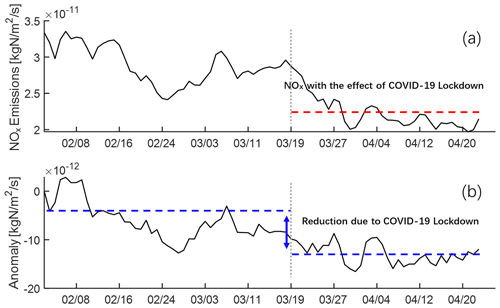
Figure 2 Satellite-derived NO_x emission estimates in southern California. (a) Daily NO_x emissions from 1 February to 23 April 2020. The red line represents the average emissions during the period after 19 March. (b) NO_x emission changes due to COVID-19 (i.e., the anomaly), which are quantified using the difference between the real-world NO_x emissions and the emissions in a hypothetical scenario without considering COVID-19. The emissions in the hypothetical scenario are estimated based on emission trends in prior years (2017–2019) using 1 February as a reference. The difference between two blue dashed lines represents the average reductions of NO_x emissions induced by the COVID-19 lockdown measures that took effect on 19 March. The local valley between 24 February and 3 March is caused by retrieval uncertainties due to unfavorable meteorology conditions and is thus excluded when we estimate the average NO_x emissions before the lockdown.

2.2 Observational data and model evaluation

We use a series of meteorology and air quality observations to evaluate the model performance and help analyze the influence of the COVID-19 lockdown. For meteorology, we use observational data obtained from the National Climatic Data Center (NCDC), from which hourly or 3 h observations of wind speed at 10 m (WS10), temperature at 2 m (T2), and water vapor mixing ratio at 2 m (Q2) are available for 82 sites distributed southern California (the red rectangle in Fig. 1). We compare the WRF-Chem meteorological simulations with these measurements and apply a number of statistical indices defined in Emery et al. (2001) to quantitatively evaluate the model performance, as summarized in Table 3. In general, the model simulations agree fairly well with surface meteorological observations. The performance statistics for WS10, T2, and Q2 are all within the benchmark ranges proposed by Emery et al. (2001).

Table 3 Evaluation of meteorological simulation results compared to observational data from the National Climatic Data Center.

^a The reference values are taken from Emery et al. (2001). ^b IOA: index of agreement.

For air quality, we achieve hourly observations of PM_2.5, O₃, NO₂, and SO₂ from CARB (California Air Resources Board, 2020) and use them to evaluate the air quality simulations of WRF-Chem (see the “Results and discussion” section). The observational data are available at 42 sites for PM_2.5, 63 sites for O₃, 48 sites for NO₂, and 12 sites for SO₂ in southern California (the red rectangle in Fig. 1) during the simulation period. We do not evaluate the model performance in simulating the chemical composition of PM_2.5 because the composition data from major observational networks were not available by the time we completed the present study. Nevertheless, our previous studies using almost the same model configurations showed fairly good agreement with PM_2.5 composition observations during January, April, July, and October 2012 (Zhao et al., 2019a; T. Y. Wang et al., 2020).

3 Results and discussion

3.1 Evaluation of the simulated results with surface observations

In this study, we simulated the major air pollutants using WRF-Chem under two scenarios, Base and Lockdown (Table 1). To evaluate the model performance with regard to the temporal variations in air pollutants, we compared the simulated concentrations of PM_2.5, maximum daily 8 h average (MDA8) O₃, NO₂, and SO₂ with observational data from CARB in southern California.

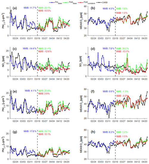
Figure 3 Time series of observed and simulated concentrations of major pollutants. (a–d) Time series of (a) PM_2.5, (b) MDA8 O₃, (c) NO₂, and (d) SO₂ averaged across all observational stations from CARB over southern California. (e–f) Time series of (e) PM_2.5 and (f) MDA8 O₃ across all stations over the urban areas of southern California. (g–h) The same as (e)–(f) but for the rural areas. Black lines are surface observations from the CARB network. Blue, green, and red lines are simulated air pollutant concentrations during the pre-lockdown period (18 February to 18 March) under the Base scenario (Pre_Base), during the lockdown period (19 March to 23 April) under the Base scenario (Post_Base), and during the lockdown period under the Lockdown scenario (Post_Lockdown). The definitions of the Base and Lockdown scenarios are summarized in Table 1. Normalized mean bias (NMB) is given by $={\sum }_{i=\mathrm{1}}^N({\mathrm{Var}}_{\mathrm{m}}-{\mathrm{Var}}_{\mathrm{o}})/{\sum }_{i=\mathrm{1}}^N{\mathrm{Var}}_{\mathrm{o}}$, where N is the number of sites, and Var_m and Var_o are modeled and observed concentrations, respectively.

Before the COVID-19 lockdown (18 February to 18 March), results from model simulations under the Base scenario (Pre_Base) capture the magnitude and temporal evolution of the four key air pollutants reasonably well, with normalized mean biases (NMBs) of 11.7 %, 4.5 %, −14.4 %, and 7.8 % for PM_2.5, MDA8 O₃, NO₂, and SO₂, respectively (Fig. 3). During the COVID-19 lockdown period (19 March to 23 April), compared to the simulations for the Base scenario (Post_Base), which overestimates the surface concentrations with NMBs of 28.1 %, 1.6 %, 21.4 %, and 39.2 % for PM_2.5, MDA8 O₃, NO₂, and SO₂, respectively, the simulated results using the adjusted emission inventory (Post_Lockdown) not only agree better with surface observations for all four air pollutants (with NMBs of 10.6 %, 1.0 %, −12.6 %, and −13.1 % for PM_2.5, MDA8 O₃, NO₂, and SO₂, respectively), but also show NMBs generally closer to those during the pre-lockdown period (Fig. 3). The improvement in model performance is observed for both urban and rural areas. In the urban areas, the NMB for PM_2.5 drops from 25.8 % under the Base scenario to 3.9 % under the Lockdown scenario, getting closer to the NMB of 4.0 % during the pre-lockdown period. The corresponding NMB in rural areas drops from 29.7 % to 15.1 %, also getting closer to 17.8 % during the pre-lockdown period (Fig. 3e, g). Regarding MDA8 O₃, although the differences between the Base and Lockdown scenarios are quite small (Fig. 3b), the NMB is slightly improved from −1.5 % (Post_Base) to −0.2 % (Post_Lockdown) in urban areas and from 3.2 % to 1.5 % in rural areas (Fig. 3f, h).

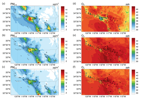
Figure 4 Overlay plots of the simulated (contour) and observed (circles) PM_2.5 and MDA8 O₃ concentrations in southern California. Panels (a)–(c) are for PM_2.5 and (d)–(f) are for MDA8 O₃. Panels (a) and (d) are for the pre-lockdown period (18 February to 18 March) under the Base scenario (Pre_Base); (b) and (e) are for the lockdown period (19 March to 23 April) under the Base scenario (Post_Base); (c) and (f) are for the lockdown period under the Lockdown scenario (Post_Lockdown).

Subsequently, we evaluated the spatial distributions of simulated PM_2.5 and MDA8 O₃ concentrations using observational data averaged during the pre-lockdown and lockdown periods in southern California (Fig. 4). Figure S4 shows the scattergrams of the simulated and observed monthly average PM_2.5 and MDA8 O₃ concentrations in southern California. The Base scenario can simulate the spatial patterns of PM_2.5 and MDA8 O₃ reasonably well (Fig. 4a–b and d–e), but it overestimates the observations of PM_2.5 concentrations during the lockdown period (Post_Base, Figs. 4b and S4b). The simulated distributions of PM_2.5 concentrations under the Lockdown scenario (Post_Lockdown) match the observations better than those for the Base scenario (Post_Base) (Figs. 4b–c and S4b–c); the hot spots occurring over Los Angeles County become less polluted and more consistent with the surface observations after considering the emission reductions associated with the COVID-19 lockdown (Fig. 4b–c).

3.2 Effects of anthropogenic emission reductions and meteorology conditions on air pollutants

Both observations and simulations in Fig. 3 show significant changes in air pollutant concentrations during the COVID-19 lockdown relative to the pre-lockdown period, resulting from a combination of emission reductions and meteorology variations. Our model simulations allow us to quantify the relative contributions of these two factors. Figure 5a–f illustrate population-weighted concentrations of simulated PM_2.5 components, NO₂, SO₂, MDA8 O₃ in southern California, and MDA8 O₃ over the urban and rural areas of southern California under the Base and Lockdown scenarios. We use population-weighted concentrations because they are more relevant to the health impacts of air pollutants (PM_2.5 and O₃), the mitigation of which is an ultimate goal of controlling air pollution. Figure S5 shows the mean concentrations of simulated PM_2.5 components, MDA8 O₃, NO_2, and SO₂ in southern California.

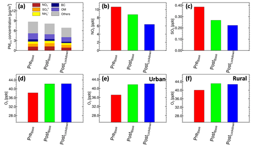
Figure 5 Effects of emission reductions and meteorology conditions on air pollutants. (a–d) Population-weighted concentrations of simulated air pollutant concentrations in southern California: (a) PM_2.5 components; (b) NO₂; (c) SO₂; (d) MDA8 O₃ over southern California; (e) MDA8 O₃ over the urban areas of southern California; (f) MDA8 O₃ over the rural areas of southern California. Pre_Base, Post_Base, and Post_Lockdown have the same meanings as in Fig. 3.

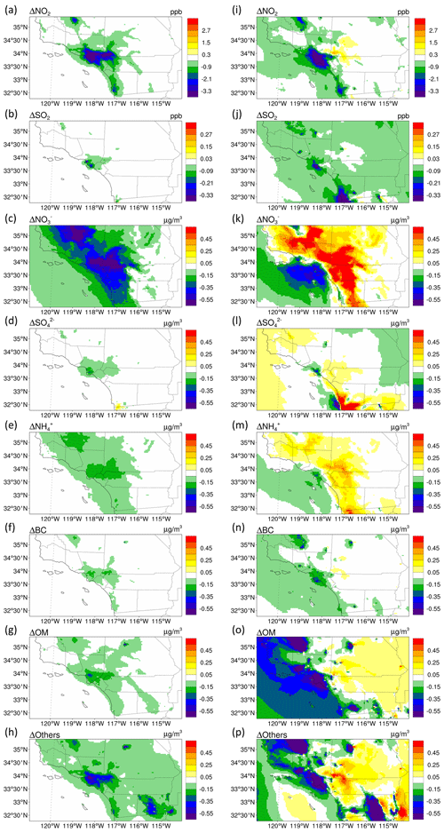
The simulations of the Base and Lockdown scenarios during the lockdown period (Post_Base and Post_Lockdown) have the same model configurations and inputs (same large-scale meteorological conditions) except for different emission inventories. The concentration differences between the two scenarios during the lockdown period (Post_Lockdown-Post_Base) represent the effect of anthropogenic emission reductions. Strictly speaking, while the large-scale meteorological fields are the same in Post_Base and Post_Lockdown, the different emission inputs could cause small differences in regional meteorology fields through the interactions between air pollutants and meteorology. Such a meteorology perturbation is considered to be part of the emission reduction effect because it is fundamentally caused by emission reductions. The simulations of the Base scenario during the lockdown and pre-lockdown periods (Post_Base and Pre_Base) both use the emission inventories without considering COVID-19-induced emission reductions. The differences between Post_Base and Pre_Base can be regarded as the impact of meteorology variations. Here our intention is to examine the relative contribution of meteorological variations to the population-weighted air pollutant concentrations before and after the lockdown instead of the changes relative to the climatological conditions. However, we acknowledge that it is more meaningful and informative to assess the meteorological effect by conducting ensemble simulations over multiple years or using multiyear averaged meteorological conditions to serve as a reference state (Le et al., 2020), which warrants further studies in the future. Figures 6 and 7 further show the spatial distribution of the concentration changes caused by anthropogenic emission reductions and meteorology variations.

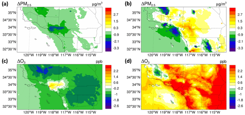
Figure 6 Spatial distributions of the emission reductions and meteorology condition effects on air pollutants. (a, c) Emission reductions and (b, d) meteorology variations in (a, b) PM_2.5 and (c, d) MDA8 O₃ concentrations.

Figure 7 The same as Fig. 6 but for NO₂, SO₂, and different PM_2.5 chemical components.

The simulated population-weighted NO₂ concentrations during the lockdown decrease by 4.3 ppb (from 10.7 to 6.4 ppb) relative to the pre-lockdown period, to which the anthropogenic emission reductions and meteorology conditions contribute 2.4 ppb (56 %) and 1.9 ppb (44 %), respectively (Fig. 5b). The decrease in NO₂ concentrations as a result of the anthropogenic emission reductions (27 %) is similar to the reduction ratio in NO_x emissions (28 %), indicating that the NO_x emission reductions can be almost fully transferred to ambient concentrations. According to our emission estimation, over 80 % of the NO_x reductions is attributed to the substantially lowered traffic intensity due to the stay-at-home order. Note that the soil NO_x emissions are not taken into account in our WRF-Chem simulation. According to Guo et al. (2020), the total soil NO_x emissions in California account for only about 1.1 % of the state's total anthropogenic NO_x emissions (California Air Resources Board, 2017). The soil NO_x emissions in southern California are generally even lower compared to other parts of the state (Guo et al., 2020). Since our study focuses on the impact of anthropogenic emission reductions on air quality during the COVID-19 lockdown period, the absence of soil NO_x emissions has little impact on our main results and will not change the main findings of this study. The population-weighted concentrations of SO₂ also show a decreasing trend (Fig. 5c). Compared with NO₂, the decrease in SO₂ concentrations due to emission reductions is smaller (17 %), partly because power generators and heavy industry (the main sources of SO₂) are less affected by the COVID-19 lockdown (see Table 2).

Coinciding with the decrease in NO₂ and SO₂, the simulated population-weighted PM_2.5 concentrations decrease by 1.8 µg m⁻³ from 8.7 µg m⁻³ during the pre-lockdown period (Pre_Base) to 6.9 µg m⁻³ during the lockdown period (Post_Lockdown). The emission reductions contribute 1.2 µg m⁻³ (67 %) of the above decrease, which translates into a 15 % reduction in population-weighted PM_2.5 concentrations from the levels without the lockdown (i.e., Post_Base) (Fig. 5a). The decrease occurs almost everywhere across the domain (Fig. 6a), consistent with the results in the last section that PM_2.5 concentrations are lowered in both urban and rural areas as a result of the emission reductions (Fig. 3e, g). The concentration decrease is higher in urban areas than in rural areas (Figs. 6a and 3e, g), with the most significant decline occurring in urban areas of Los Angeles County (Fig. 6a). In contrast, the meteorology variations can increase the PM_2.5 concentrations in some regions (mainly the inland regions) and decrease them in others (mainly the coastal regions) (Fig. 6b). The net effect is to reduce the population-weighted concentration by 0.6 µg m⁻³ since the concentration decrease happens to occur in more densely populated regions (Fig. 5a).

The concentrations of PM_2.5 are affected by emissions of multiple pollutants through both primary emissions and chemical reactions. To further explore the reasons behind the PM_2.5 concentration changes, we examine the changes in individual chemical components, as shown in Figs. 5a and 7. Following the emission changes (from Post_Base to Post_Lockdown), all major PM_2.5 components experience a concentration decrease throughout almost the entire domain (Fig. 7), since the emissions of essentially all pollutants are reduced to some extent due to the lockdown measures (Table 2). The population-weighted concentrations of nitrate decrease the most (0.42 µg m⁻³), followed by “others” (0.32 µg m⁻³, including all other components besides the key components listed here), organic matter (OM, 0.16 µg m⁻³), ammonium (0.15 µg m⁻³), black carbon (BC, 0.10 µg m⁻³), and sulfate (from 0.07 µg m⁻³) (Fig. 5a). The largest decrease in nitrate is tied to the substantial reduction in NO_x emissions, which is further explained by a larger reduction ratio in transportation emissions (by 30 %–70 %) compared to other emission sources (Table 2). In addition, the decreases in others, elemental carbon (EC), and primary OM (a fraction of the total OM) are attributable to the reductions in primary PM_2.5 emissions. In our emission estimates, the sector-specific relative emission changes of EC, primary OM, and others are assumed to be the same as the total primary PM_2.5, as summarized in Table 2. For the total emissions of all sectors, the reductions in EC, primary OM, and others are 22.7 %, 15.8 %, and 13.5 %, respectively, which are slightly different from the reduction in total primary PM_2.5 since different chemical components have different sectoral distributions. The overall concentration decrease in these primary chemical components even exceeds that of nitrate; this clearly indicates an important role of primary PM_2.5 components in improving PM_2.5 air quality during the lockdown period, although the primary PM_2.5 emissions have only been reduced by 15 %.

The simulated population-weighted O₃ concentrations increase noticeably from 38 ppb in the pre-lockdown period (Pre_Base) to 42 ppb (Post_Lockdown) during the lockdown, and the effects of meteorological changes (i.e., Post_Base−Pre_Base) play a dominant role in the variation of O₃. The O₃ level is strongly affected by ambient conditions like temperature and solar radiation (Z. Wang et al., 2015). As the temperature gets warmer and the radiation gets stronger over time, the O₃ concentrations are elevated in most areas during the COVID-19 lockdown compared to the pre-lockdown period (Fig. 6d). The emission reductions cause an O₃ decrease in rural areas but a slight increase in the urban areas (Figs. 6c and 3f, h), which is consistent with previous findings (Zhao et al., 2019a; T. Y. Wang et al., 2020; Martien et al., 2003; Qin et al., 2004). In urban areas where NO_x emissions are high, a volatile-organic-compound-limited (VOC-limited) regime is seen, while in rural areas, a NO_x-limited regime is observed (Martien et al., 2003; Qin et al., 2004). It follows that the decrease in NO_x emissions leads to opposite changes in O₃ concentrations in urban and rural areas. The increase and decrease in different areas largely offset each other, resulting in a negligible change in population-weighted O₃ concentrations (0.07 ppb) (Fig. 5d) and a slight decrease in area-averaged O₃ concentrations over the modeling domain (0.77 ppb) (Figs. 6c and S5b). Last but not least, the small sensitivity of O₃ to emission reductions is also partly explained by the fact that 75 % of the ambient O₃ concentration is background O₃ (Zhao et al., 2019a; T. Y. Wang et al., 2020).

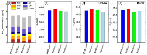
Figure 8 Simulated population-weighted PM_2.5 and O₃ concentrations under three sensitivity scenarios (VOC1.0, NO_x0.3, and VOC0.3) during the lockdown period (19 March to 23 April) over southern California. (a) PM_2.5 components, (b) MDA8 O₃, and (c) MDA8 O₃ over the urban areas, as well as (d) MDA8 O₃ over the rural areas. The definitions of all scenarios are summarized in Table 1.

3.3 Effects of anthropogenic NO_x and VOC emission reductions on ozone concentration

Our modeling results showed an increase in O₃ in urban areas due to the emission reductions in association with the lockdown during the COVID-19 pandemic. The O₃ concentrations are most significantly affected by emissions of NO_x and VOCs (Stewart et al., 2017). To further explore the drivers of the O₃ changes and potential approaches to effectively reduce O₃ concentrations, we conduct three sensitivity experiments involving NO_x and VOC emission perturbations, as summarized in Table 1. Figure 8 illustrates population-weighted concentrations of simulated PM_2.5 components and MDA8 O₃ after the COVID-19 lockdown under these sensitivity scenarios. Figure 9 shows the spatial distribution of the differences in MDA8 O₃ between the sensitivity scenarios and the Base scenario. Figure 10 shows the concentration time series for the sensitivity scenarios. The first sensitivity experiment is the VOC1.0 scenario, which is the same as Lockdown except that the VOC emissions are kept at the level of the Base scenario (Table 1). This scenario, in combination with the Base and Lockdown scenarios, can be used to evaluate the response of O₃ concentrations if the COVID-19-induced emission reductions of NO_x and VOC were implemented in sequence. Without the control of VOC emissions in VOC1.0 (Fig. 9a), the increase in urban O₃ concentration relative to the Base scenario becomes larger than the Lockdown scenario (Fig. 6c). This confirms our conclusion in the last section that the NO_x emission control elevates urban O₃ concentrations under the VOC-limited regime and meanwhile indicates that the VOC control is conducive to O₃ decrease. To assess the potential effects of strengthened NO_x and VOC control measures, we conduct two other sensitivity experiments named NO_x0.3 and VOC0.3, which are the same as Lockdown except that the anthropogenic NO_x (for the NO_x0.3 scenario) and VOC (for the VOC0.3 scenario) emissions are further reduced to 30 % of those in the Base scenario. As a 70 % reduction is close to the maximum reductions in NO_x and VOC emissions that could be achieved through the full implementation of technologically and economically feasible control measures (Amann et al., 2020), we select an emission ratio of 0.3 (70 % reduction) to represent the potential impact of highly stringent control policies in the future. Figure 8a and b show that strengthened NO_x control further reduces the population-weighted concentrations of PM_2.5, while further reduction of anthropogenic VOCs helps to decrease the concentration of MDA8 O₃. Differences in O₃ concentration clearly illustrate different spatial distribution patterns for urban and suburb areas (Fig. 9b, c). For the suburbs with high O₃ values, reducing anthropogenic NO_x and VOCs is conducive to the decline of O₃ (Fig. 8d). For urban areas, however, strengthened control with anthropogenic NO_x reduced by 70 % (NO_x0.3) results in even more O₃ increase in the central urban area (Figs. 9b and 8c). Amplified ozone pollution has also been reported by Sicard et al. (2020) based on their observational studies in four southern European cities and Wuhan, China, associated with NO_x reductions in response to COVID-19. To control O₃ concentrations in urban areas, VOC control may be an effective method. While a NO_x emission reduction might cause an increase in O₃ concentration, a VOC reduction generally leads to a monotonous reduction of O₃ concentrations regardless of the O₃ formation regime, as indicated by the classical O₃ EKMA isopleth (Fig. 6-1 of National Research Council, 1991, or Fig. 3.2.1 of Donahue, 2018) as well as some recent studies in southern California (Fujita et al., 2013; Collet et al., 2018; Qian et al., 2019). We find that in the VOC0.3 scenario, there is almost no O₃ concentration increase relative to the Base scenario, in contrast to a significant urban O₃ increase in the Lockdown scenario (Fig. 9c). This means that a 70 % reduction in anthropogenic VOCs can offset the increases in O₃ caused by the 28.3 % NO_x reduction during the lockdown. Note that we are specifically looking at the extent of VOC emission reductions that are needed to offset the 28.3 % NO_x reduction caused by the lockdown, which minimizes the complexity due to the nonlinear O₃ responses when the NO_x emissions change simultaneously. Furthermore, Wang et al. (2019) found that 75 % of the average O₃ concentration in California was due to distant emissions outside the western United States. Many other studies have also revealed that background O₃ dominates over the contribution from local emissions in the western US (Huang et al., 2015; Oltmans et al., 2008; Fiore et al., 2014; Emery et al., 2012; Zhang et al., 2011). Therefore, cooperating with other regions and countries in emission reductions may be another way to control O₃ in urban areas of southern California.

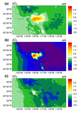
Figure 9 Spatial distribution of the differences in MDA8 O₃ between the three sensitivity scenarios and the Base scenario: (a) VOC1.0 minus Base; (b) NO_x0.3 minus Base; (c) VOC0.3 minus Base. The definitions of all scenarios are summarized in Table 1.

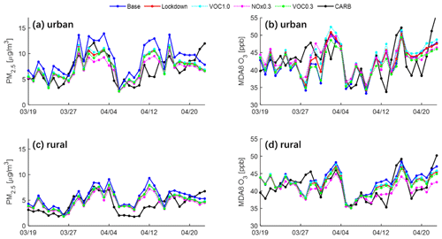
Figure 10 Time series of simulated and observed PM_2.5 concentrations (a, c) and MDA8 O₃ concentrations (b, d) under several sensitivity scenarios averaged across the CARB observational stations over the urban (a, b) and rural (c, d) areas of southern California during the lockdown period (19 March to 23 April). Black lines are surface observations from CARB networks. Blue, red, cyan, magenta, and green lines are simulated results for the Base, Lockdown, VOC1.0, NO_x0.3, and VOC0.3 scenarios. The definitions of all scenarios are summarized in Table 1.

4 Conclusion and policy implications

In this study, we investigated the air quality impact of emission reductions in southern California in association with COVID-19 by employing WRF-Chem to conduct high-resolution atmospheric modeling during 18 February to 23 April 2020.

Based on the statistics of activity levels, we first adjusted the emission inventory considering the emission reductions during the COVID-19 lockdown. The adjusted emission inventory is shown to be consistent with the emission inventory based on satellite observations. The simulated magnitude and temporal evolution of the concentrations of the key air pollutants, including PM_2.5, NO₂, SO₂, and MDA8 O₃, using the adjusted emission inventory agree better with surface observations than simulation results without considering the COVID-19-induced emission reductions. Due to the reduced emissions, the population-weighted concentrations of NO₂ and PM_2.5 decreased by 27 % and 15 %, respectively, in southern California in the 5 weeks after the stay-at-home orders. Emission reductions and meteorological variations contributed about two-thirds and one-third, respectively, to the total decrease in population-weighted PM_2.5 concentrations before and after the lockdown. For O₃ concentration, however, the COVID-19-related emission reductions caused a decrease in suburb areas but a slight increase in the urban areas. In order to further explore the effects of anthropogenic NO_x and VOC emission reductions on O₃ concentration, we conducted sensitivity experiments by strengthening VOC and NO_x controls. Our results showed that strengthened control with NO_x reduced by 70 % (NO_x0.3) results in even more O₃ increase in the central urban area, and anthropogenic VOC control may be an effective method to reduce O₃ concentrations in urban areas. A 70 % reduction in anthropogenic VOCs can effectively offset all the increases in O₃ caused by NO_x reduction during the lockdown.

Using COVID-19 as an unprecedented experiment with substantial emission reductions from multiple sectors, especially transportation, this study helps to elucidate the complex and nonlinear response of chemical compositions to air pollution control measures and thus provides important insight into the development and optimization of effective air pollution control strategies in southern California. We find that the reduced NO_x emissions (∼ 28 %) have been almost fully transferred to the reduction in the ambient concentration of NO₂ (∼ 27 %). This further translates into a remarkable reduction in nitrate, which makes the largest contribution to the PM_2.5 concentration decrease among all individual chemical components. Therefore, to alleviate PM_2.5 pollution, measures focusing on sectors such as transportation, which is among the main sources of NO_x emissions, could be effective. Moreover, we find that a moderate 15 % reduction of primary PM_2.5 emissions has resulted in a substantial reduction in ambient PM_2.5 concentrations, with the total concentration decreases in all primary PM_2.5 components exceeding that of nitrate. Therefore, a strengthened control on primary PM_2.5 emissions could be an effective strategy to sustainably mitigate PM_2.5 pollution. For O₃, reduction of NO_x can effectively reduce high O₃ concentrations in suburban areas but may cause an increase in urban concentrations. A 70 % VOC emission reduction is found to fully offset the urban O₃ increase caused by the lockdown. Therefore, the reduction in NO_x emissions needs to be accompanied by a well-balanced reduction in VOC emissions to avoid side effects on urban O₃ pollution.