Uncertainties in eddy covariance air–sea CO₂ flux measurements and implications for gas transfer velocity parameterisations

Air–sea carbon dioxide (CO₂) flux is often indirectly estimated by the bulk method using the air–sea difference in CO₂ fugacity (ΔfCO₂) and a parameterisation of the gas transfer velocity (K). Direct flux measurements by eddy covariance (EC) provide an independent reference for bulk flux estimates and are often used to study processes that drive K. However, inherent uncertainties in EC air–sea CO₂ flux measurements from ships have not been well quantified and may confound analyses of K. This paper evaluates the uncertainties in EC CO₂ fluxes from four cruises. Fluxes were measured with two state-of-the-art closed-path CO₂ analysers on two ships. The mean bias in the EC CO₂ flux is low, but the random error is relatively large over short timescales. The uncertainty (1 standard deviation) in hourly averaged EC air–sea CO₂ fluxes (cruise mean) ranges from 1.4 to 3.2 $\mathrm{mmol}{\mathrm{m}}^{-\mathrm{2}}{\mathrm{d}}^{-\mathrm{1}}$. This corresponds to a relative uncertainty of ∼ 20 % during two Arctic cruises that observed large CO₂ flux magnitude. The relative uncertainty was greater (∼ 50 %) when the CO₂ flux magnitude was small during two Atlantic cruises. Random uncertainty in the EC CO₂ flux is mostly caused by sampling error. Instrument noise is relatively unimportant. Random uncertainty in EC CO₂ fluxes can be reduced by averaging for longer. However, averaging for too long will result in the inclusion of more natural variability. Auto-covariance analysis of CO₂ fluxes suggests that the optimal timescale for averaging EC CO₂ flux measurements ranges from 1 to 3 h, which increases the mean signal-to-noise ratio of the four cruises to higher than 3. Applying an appropriate averaging timescale and suitable ΔfCO₂ threshold (20 µatm) to EC flux data enables an optimal analysis of K.

1 Introduction

Since the Industrial Revolution, atmospheric CO₂ levels have risen steeply due to human activities (Broecker and Peng, 1998). The ocean plays a key role in the global carbon cycle, having taken up roughly one-quarter of anthropogenic CO₂ emissions over the last decade (Friedlingstein et al., 2020). Accurate estimates of air–sea CO₂ flux are vital to forecast climate change and to quantify the effects of ocean CO₂ uptake on the marine biosphere.

Air–sea CO₂ flux (F, e.g. in $\mathrm{mmol}{\mathrm{m}}^{-\mathrm{2}}{\mathrm{d}}^{-\mathrm{1}}$) is typically estimated indirectly by the bulk equation:

$$\begin{array}{}\text{(1)}& F=K_{\mathrm{660}}(\mathit{Sc}/\mathrm{660}{)}^{-\mathrm{0.5}}\mathit{\alpha }(f{\mathrm{CO}}_{\mathrm{2}\mathrm{w}}-f{\mathrm{CO}}_{\mathrm{2}\mathrm{a}}),\end{array}$$

where K₆₆₀ (in cm h⁻¹) is the gas transfer velocity, usually parameterised as a function of wind speed (e.g. Nightingale et al., 2000); Sc (dimensionless) is the Schmidt number (Wanninkhof, 2014); and α ($\mathrm{mol}{\mathrm{L}}^{-\mathrm{1}}{\mathrm{atm}}^{-\mathrm{1}}$) is the solubility (Weiss, 1974). Sc is equal to 660 for CO₂ at 20 ^∘C and 35 ‰ saltwater (Wanninkhof et al., 2009). fCO_2w and fCO_2a are the CO₂ fugacity (in µatm) at the sea surface and in the overlying atmosphere, respectively, with fCO_2w−fCO_2a the air–sea CO₂ fugacity difference (ΔfCO₂). Uncertainties in the K₆₆₀ parameterisation and limited coverage of fCO_2w measurements result in considerable uncertainties in global bulk flux estimates (Takahashi et al., 2009; Woolf et al., 2019).

Eddy covariance (EC) is the most direct method for measuring the air–sea CO₂ flux F:

$$\begin{array}{}\text{(2)}& F=\mathit{\rho }\stackrel{\mathrm{‾}}{w^{\prime }{c}^{\prime }},\end{array}$$

where ρ is the mean mole density of dry air (e.g. in mol m⁻³). The dry CO₂ mixing ratio c (in ppm or µmol mol⁻¹) is measured by a fast-response gas analyser, and the vertical wind velocity w (in m s⁻¹) is often measured by a sonic anemometer. The prime denotes the fluctuations from the mean, while the overbar indicates time average. Equation (2) does not rely on ΔfCO₂ measurements, nor empirical parameters and assumptions of the gas properties (Wanninkhof, 2014). EC flux measurements can therefore be considered useful as an independent reference for bulk air–sea CO₂ flux estimates. Furthermore, the typical temporal and spatial scales of EC flux measurements are ca. hourly and 1–10 km². These scales are much smaller than the temporal and spatial scales of alternative techniques for measuring gas transfer, e.g. by dual tracer methods (daily and 1000 km²) (Nightingale et al., 2000; Ho et al., 2006). EC measurements are thus potentially better suited to capture variations in gas exchange due to small-scale processes at the air–sea interface (Garbe et al., 2014).

The EC CO₂ flux method has developed and improved over time. Before 1990, EC was successfully used to measure air–sea momentum and heat fluxes. EC air–sea CO₂ flux measurements made during those times were unreasonably high (Jones and Smith, 1977; Wesely et al., 1982; Smith and Jones, 1985; Broecker et al., 1986). After 1990, with the development of the infrared gas analyser, EC became routinely used for terrestrial carbon cycle research (Baldocchi et al., 2001). Development of the EC method was accompanied by improvements in the flux uncertainty analysis, which was generally based on momentum, heat and land–atmosphere gas flux measurements (Lenschow and Kristensen, 1985; Businger, 1986; Lenschow et al., 1994; Wienhold et al., 1995; Mahrt, 1998; Finkelstein and Sims, 2001; Loescher et al., 2006; Rannik et al., 2009, 2016; Billesbach, 2011; Mauder et al., 2013; Langford et al., 2015; Post et al., 2015).

In the late 1990s, the advancement in motion correction of wind measurements (Edson et al., 1998; Yelland et al., 1998) facilitated ship-based EC CO₂ flux measurements from a moving platform (McGillis et al., 2001; 2004). After 2000, a commercial open-path infrared gas analyser LI-7500 (Li-COR Inc. USA) became widely used for air–sea CO₂ flux measurements (Weiss et al., 2007; Kondo and Tsukamoto, 2007; Prytherch et al., 2010; Edson et al., 2011; Else et al., 2011; Lauvset et al., 2011). The LI-7500 generated extremely large and highly variable CO₂ fluxes in comparison to expected fluxes (Kondo and Tsukamoto, 2007; Prytherch et al., 2010; Edson et al., 2011; Else et al., 2011; Lauvset et al., 2011). This problem is generally considered to be an artefact caused by water vapour cross-sensitivity (Kohsiek, 2000; Prytherch et al., 2010; Edson et al., 2011; Landwehr et al., 2014). Mathematical corrections proposed to address this artefact (Edson et al., 2011; Prytherch et al., 2010) were later shown to be unsatisfactory (Else et al., 2011; Ikawa et al., 2013; Blomquist et al., 2014; Tsukamoto et al., 2014) or incorrect (Landwehr et al., 2014).

The most reliable method for measuring EC air–sea CO₂ fluxes involves the physical removal of water vapour fluctuations from the sampled air. The simplest approach is to combine a closed-path gas analyser with a physical dryer to eliminate most of the water vapour fluctuation (Miller et al., 2010; Blomquist et al., 2014; Landwehr et al., 2014; Yang et al., 2016; Nilsson et al., 2018). The tuneable-diode-laser-based cavity ring-down spectrometer (CRDS) made by Picarro Inc. (Santa Clara, California, USA) is the most precise closed-path analyser currently available (Blomquist et al., 2014). The closed-path infrared gas analyser LI-7200 (LI-COR Biosciences, Lincoln, Nebraska, USA) is another popular choice.

The advancements in instrumentation and in motion correction methods have significantly improved the quality of air–sea EC CO₂ flux observations, but, despite these changes, the flux uncertainties have not been well quantified. The aims of this study are to (1) analyse uncertainties in EC air–sea CO₂ flux measurements; (2) propose practical methods to reduce the systematic and random flux uncertainty; and (3) investigate how the EC flux uncertainty influences our ability to estimate and parameterise K₆₆₀.

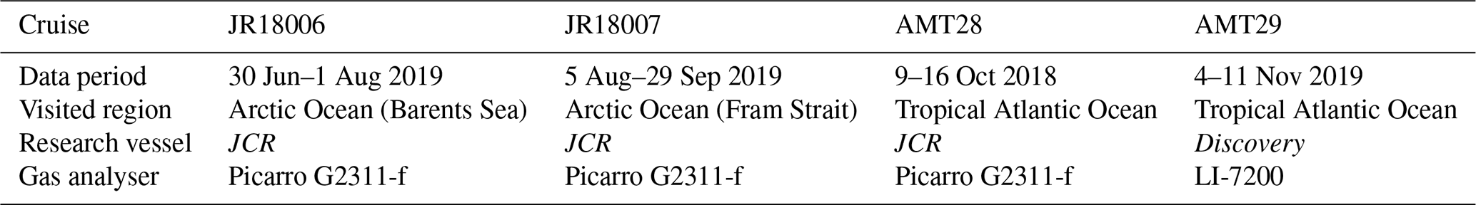
Table 1 Basic information for all four cruises on the RRS James Clark Ross (JCR) and RRS Discovery that measured air–sea EC CO₂ fluxes.

2 Experiment and methods

2.1 Instrumental setup

The basic information of four cruises is summarised in Table 1. Appendix A shows the four cruise tracks (Figs. A1 and A2). Data from the Atlantic cruises (AMT28 and AMT29) are limited to 3^∘ N–20^∘ S in order to focus specifically on the performance of two different gas analysers in the same region with low flux signal (tropical zone).

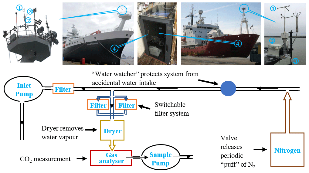
Figure 1 EC system (upper panel) and a diagram of the system setup (bottom panel). EC instruments: (1) sonic anemometer, (2) motion sensor, (3) air sample inlet for gas analyser, (4) data logger/gas analyser. Arctic and Atlantic data from 2018 were collected on the RRS James Clark Ross (JCR; upper right) using a Picarro G2311-f, and Atlantic data from 2019 were collected using a LI-7200 on the RRS Discovery (upper left).

The CO₂ flux and data logging systems installed on the JCR and Discovery were operated autonomously. The EC systems were approximately 20 $\mathrm{m}\mathrm{a}.\mathrm{m}.\mathrm{s}.\mathrm{l}.$ on both ships (at the top of the foremasts; Fig. 1) to minimise flow distortion and exposure to sea spray. Computational fluid dynamics (CFD) simulation indicates that the airflow distortion at the top of the JCR foremast is small (∼ 1 % of the free stream wind speed when the ship is head to wind; Moat and Yelland, 2015). The hull structure of RRS Discovery is nearly identical to that of RRS James Cook. CFD simulation of the James Cook indicates that the airflow at the top foremast is distorted by ∼ 2 % for bow-on flows (Moat et al., 2006). The deflection of the streamline from horizontal and effects on the vertical wind component is accounted for by the double rotation (motion correction processes; see Sect. 2.2) prior to the EC flux calculation for both ships.

The EC system on the JCR consists of a three-dimensional sonic anemometer (Metek Inc., Sonic-3 Scientific), a motion sensor (initially Systron Donner Motionpak II, which compared favourably with and was then replaced by a Life Performance-Research LPMS-RS232AL2 in April 2019), and a Picarro G2311-f gas analyser. All instruments sampled at a frequency of 10 Hz or greater, and the data were logged at 10 Hz with a data logger (CR6, Campbell Scientific, Inc.), similar to the setup by Butterworth and Miller (2016). Air is pulled through a long tube (30 m, inner diameter 0.95 cm, Reynolds number 5957) with a dry vane pump at a flow rate of ∼ 40 L min⁻¹ (Gast 1023 series). The Picarro gas analyser subsamples from this tube through a particle filter (Swagelok 2 µm) and a dryer (Nafion PD-200T-24M) at a flow of ∼ 5 L min⁻¹ (Fig. 1). The dryer is set up in the “re-flux” configuration and uses the lower pressure Picarro exhaust to dry the sample air. This method removes ∼ 80 % of the water vapour and essentially all of the humidity fluctuations (Yang et al., 2016). The Picarro internal calculation accounts for the detected residual water vapour and yields a dry CO₂ mixing ratio that is used in the flux calculations. A valve controlled by the Picarro instrument injects a “puff” of nitrogen (N₂) into the tip of the inlet tube for 30 s every 6 h. This enables estimates of the time delay and high-frequency signal attenuation (Sect. 2.2).

The EC system on RRS Discovery consists of a Gill R3-50 sonic anemometer, a LPMS motion sensor package, and a LI-7200 gas analyser. The LI-7200 gas analyser was mounted within the enclosed staircase, directly underneath the meteorological platform and close to the inlet (inlet length 7.5 m, inner diameter 0.95 cm, Reynolds number 1042). A single pump (Gast 1023) was sufficient to pull air through a particle filter (Swagelok 2 µm), a dryer (Nafion PD-200T-24M), and the LI-7200 at a flow of ∼ 7 L min⁻¹. There was no N₂ puff system setup on Discovery, but equivalent lab tests confirmed that the delay time was less than on the JCR because of the shorter inlet line. The dryer on the Discovery is set up in the same re-flux configuration as the JCR and uses the lower pressure at the LI-7200 exhaust (limited by an additional 0.08 cm diameter critical orifice) to dry the sample air. This setup removes ∼ 60 %–70 % of the water vapour and essentially all of the humidity fluctuations. The dry CO₂ mixing ratio, computed by accounting for the LI-7200 temperature, pressure, and residual water vapour measurements, is used in the flux calculations.

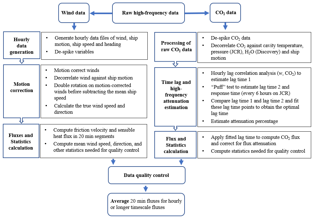
Figure 2 Flow chart of EC data processing. The raw high-frequency (10 Hz) wind and CO₂ data were initially processed separately and then combined to calculate fluxes. CO₂ fluxes were filtered by a series of data quality control criteria. The 20 min flux intervals were averaged to longer timescales (hourly or more). The data processing is detailed in the text.

2.2 Flux processing

The EC air–sea CO₂ flux calculation steps using the raw data are outlined with a flow chart (Fig. 2) and detailed below. The raw high-frequency wind and CO₂ data are processed first, yielding fluxes in 20 min averaging time interval and related statistics. These statistics are then used for quality control of the fluxes. Further averaging of the quality-controlled 20 min fluxes to hourly or longer timescales is then used to reduce random error (Sect. 4.1). Linear detrending was used to identify the turbulent fluctuations (i.e. w^′ and c^′) throughout the analyses.

To correct the wind data for ship motion, we first generated hourly data files containing the measurements from the sonic anemometer (three-dimensional wind speed components: u, v, and w and sonic temperature T_s), motion sensor (three axis accelerations: accel_x, accel_y, accel_z; and rotation angles: rot_x, rot_y, rot_z), ship heading over ground (HDG; from the gyro compass), and ship speed over ground (SOG; from Global Position System). Spikes larger than 4 standard deviations (SDs) from the median were removed. Secondly, a complementary filtering method using Euler angles (see Edson et al., 1998) was applied to the hourly data files to remove apparent winds generated by the ship movements. The motion-corrected winds were further decorrelated against ship motion to remove any residual motion-sensitivity (Miller et al., 2010; Yang et al., 2013). The motion-corrected winds were double-rotated to account for the wind streamline over the ship, yielding the vertical wind velocity (w) required in Eq. (2). Inspection of frequency spectra showed that the spectral peak at the ship motion frequencies (approximately 0.1–0.3 Hz) had disappeared after the motion correction (Fig. S1 in the Supplement). This indicates that the majority of ship motion had been removed from the measured wind speed. The last step in the wind data processing was the calculation of 20 min average friction velocity, sensible heat flux, and other key variables used for data quality control (Table S1 in the Supplement).

The CO₂ data were de-spiked (by removing values > 4 SDs from the median). The Picarro CO₂ mixing ratio was further decorrelated against analyser cell pressure and temperature to remove CO₂ variations due to the ship's motion. The LI-7200 CO₂ mixing ratio was further decorrelated against the LI-7200 H₂O mixing ratio and temperature to remove residual air density fluctuations, following Landwehr et al. (2018). CO₂ data were also decorrelated against the ship's heave and accelerations because these can produce spurious CO₂ variability (Miller et al., 2010; Blomquist et al., 2014).

A lag between CO₂ data acquisition and the wind data is created because of the time taken for sample air to travel through the inlet tube. On the JCR, we use the puff system where the lag time is the time difference between the N₂ puff start (when the on/off valve is switched) and the time when the diluted signal is sensed by the gas analyser. The lag time can also be estimated by the maximum covariance method, calculated by shifting the time base of the CO₂ signal and finding the shift that achieves maximum covariance between the vertical wind velocity (w) signal and the shifted CO₂ signal. The lag times estimated by the maximum covariance method agree well with the estimates of the puff procedure (Fig. S2 in the Supplement). These estimates indicate a lag time of 3.3–3.4 s for the Arctic cruises and 3.3 s for cruise AMT28 on the JCR. The lag time on Discovery (AMT29) estimated by the maximum covariance method was 2.6 s, consistent with laboratory test results prior to the cruise.

The inlet tube, particle filter, and dryer cause high-frequency CO₂ flux signal attenuation. The N₂ puff was also used to assess the response time by considering the e-folding time in the CO₂ signal change (similar approaches have been used by Bariteau et al., 2010; Blomquist et al., 2014, Bell et al., 2015). The response time is 0.35 s for the EC system on JCR and 0.25 s for the EC system on Discovery (estimated in the laboratory prior to cruise). These response times were combined with the relative wind speed-dependent, theoretical shapes of the cospectra (Kaimal et al., 1972) to estimate the percentage flux loss due to the inlet attenuation (Yang et al., 2013). The mean attenuation percentage is less than 10 %, with a relative wind speed dependence (Fig. S3 in the Supplement). The attenuation percentage value was applied to the computed flux to compensate for the flux loss due to the high-frequency signal attenuation. Finally, horizontal CO₂ fluxes and other statistics such as CO₂ range and CO₂ trend were computed for quality control purposes (Table S1, Supplement).

The computed 20 min fluxes were filtered for non-ideal ship manoeuvres or violations of the homogeneity/stationary requirement of EC (see Supplement for the quality control criteria).

2.3 Uncertainty analysis methods

2.3.1 Uncertainty components

Uncertainty contains two components: systematic error (δF_S) and random error (δF_R). According to propagation of uncertainty theory (JCGM, 2008), the total uncertainty in EC CO₂ fluxes (from random and systematic errors) can be expressed as

$$\begin{array}{}\text{(3)}& \mathit{\delta }F=\sqrt{\mathit{\delta }{F}_{\mathrm{R}}^{\mathrm{2}}+\mathit{\delta }{F}_{\mathrm{S}}^{\mathrm{2}}}.\end{array}$$

Systematic errors (Sect. 2.3.2) will cause bias in the flux. They thus should be eliminated/minimised with the appropriate system setup and, if needed, effective numerical corrections. Random error results in imprecision (but not bias) and can be reduced by averaging repeated measurements (Sect. 2.3.3). Errors due to insufficient sampling and instrument noise are generally considered most important in EC flux measurements (Lenschow and Kristensen, 1985; Businger, 1986; Mauder et al., 2013; Rannik et al., 2016).

Sampling error is an inherent issue for EC flux measurements and is typically the main source of the CO₂ flux uncertainty (Mauder et al., 2013). The sampling error is caused by the difference between the ensemble average and the time average. The calculation of EC flux (Eq. 2) requires the separation between the mean and fluctuating components, which can be represented fully for CO₂ mixing ratio c as

$$\begin{array}{}\text{(4)}& c(x,t)=\stackrel{\mathrm{‾}}{c}(x,t)+c^{\prime }(x,t).\end{array}$$

The mean component $\stackrel{\mathrm{‾}}{c}$ represents ensemble average over time (t) and space (x) and does not contribute to the flux. The time average of a stationary turbulent signal and space average of a homogenous turbulent signal theoretically converge on the ensemble average when the averaging time approaches infinity, i.e. T→∞ (Wyngaard, 2010). In practice, Reynolds averaging over a much shorter time interval (10 min to an hour) is typically used for EC flux measurements from a fixed point or from a slow-moving platform such as a ship. This is because the atmospheric boundary layer is only quasi-stationary for a few hours. Non-stationarity (e.g. diurnal variability and synoptic conditions) is an inherent property of the atmospheric boundary layer (Wyngaard, 2010). EC flux observations thus inevitably contain some random error due to insufficient sampling time, and this error is greater at shorter averaging times.

Random error due to instrument noise comes mainly from the white noise of the gas analyser, as the noise from the sonic anemometer is relatively unimportant (Blomquist et al., 2010; Fairall et al., 2000; Mauder et al., 2013). Blomquist et al. (2014) show “pink” noise with a weak spectral slope for their CRDS gas analyser (G1301-f), but the gas analysers on JCR (G2311-f) and Discovery (LI-7200) demonstrate white noise with a constant variance at high frequency (Fig. B2, Appendix B).

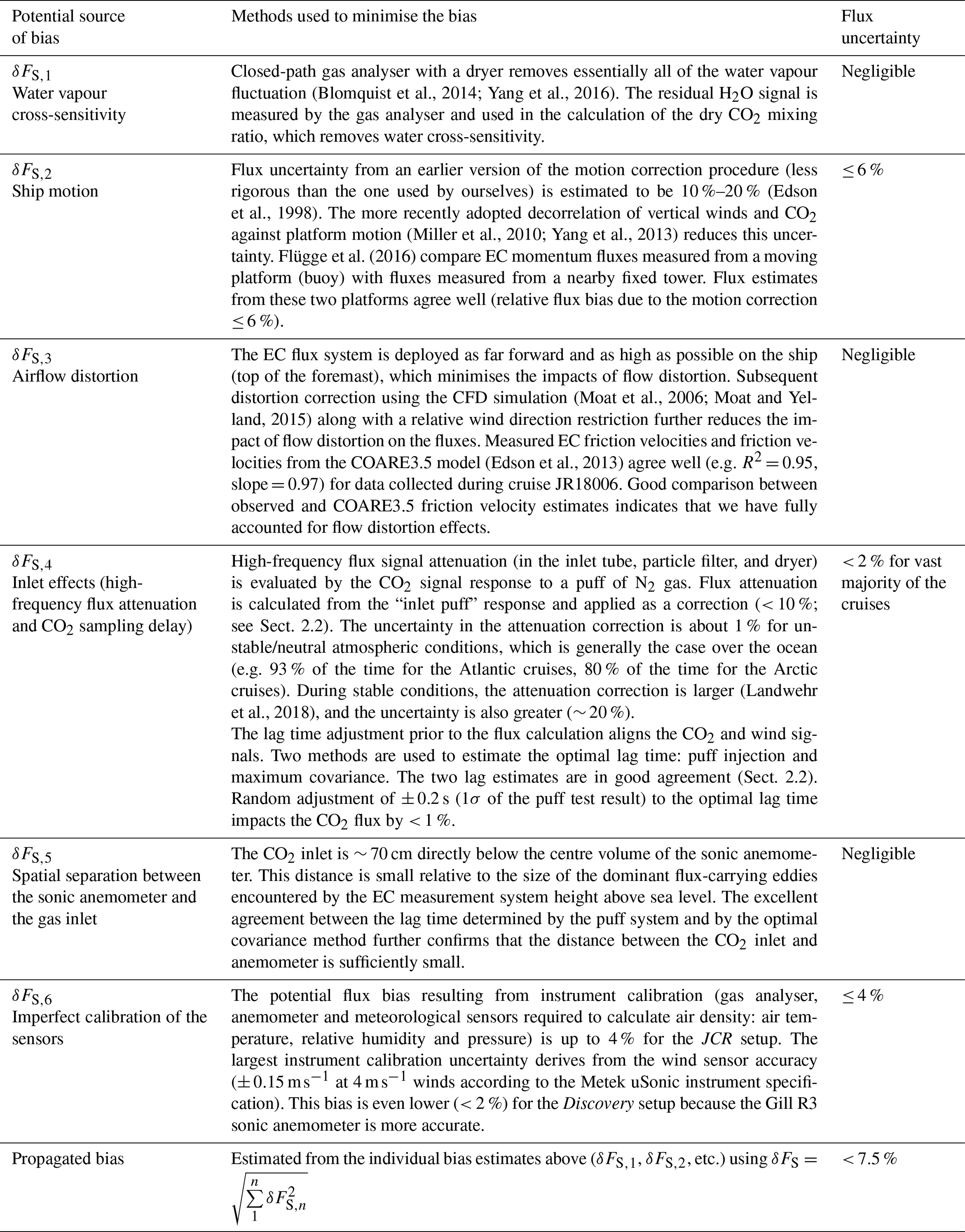
Table 2 Potential sources of bias in our EC air–sea CO₂ flux measurements and the methods used to minimise them.

2.3.2 Systematic error

Table 2 details the measures taken during instrument setup and data processing that help eliminate most sources of systematic error in EC CO₂ fluxes.

In addition to bias sources related to the instrument setup (Table 2), insufficient sampling time (an inherent issue of EC fluxes) may also generate a systematic error. We use a theoretical method to estimate this systematic error in EC CO₂ flux (Lenschow et al., 1994):

$$\begin{array}{}\text{(5)}& \mathrm{|}\mathit{\delta }{F}_{\mathrm{S}}\mathrm{|}\le \mathrm{2}{\mathit{\sigma }}_{\mathrm{w}}{\mathit{\sigma }}_{{\mathrm{c}}_{\mathrm{a}}}{\displaystyle \frac{\sqrt{{\mathit{\tau }}_{\mathrm{w}}{\mathit{\tau }}_{\mathrm{c}}}}{T}},\end{array}$$

where σ_w (m s⁻¹) and ${\mathit{\sigma }}_{{\mathrm{c}}_{\mathrm{a}}}$ (ppm) are the standard deviations of the vertical wind velocity and the CO₂ mixing ratio due to atmospheric processes, respectively. T is the averaging time interval (s), and τ_w and τ_c are integral timescales (s) for vertical wind velocity and CO₂ signal, respectively. The definition and estimation of the integral timescale are shown in Appendix B. The sign of δF_S could be positive or negative (i.e. under- or overestimation) because of the poor statistics in capturing low-frequency eddies within the flux averaging period (Lenschow et al., 1993). The mean hourly relative systematic error due to insufficient sampling time for four cruises estimated by Eq. (5) is < 5 %. According to propagation of uncertainty theory (JCGM, 2008), the total systematic error is less than 9 % (= $\sqrt{\mathrm{7.5}{\mathit{\%}}^{\mathrm{2}}+\mathrm{5}{\mathit{\%}}^{\mathrm{2}}}$).

2.3.3 Random error

Five approaches used to estimate the total random error (A–C) and the random error component due to instrument noise (C–E) in EC CO₂ fluxes are discussed below. The random error assessments are empirical (A and D) or theoretical (B, C, and E).

• A.

  An empirical approach to estimate total random error involves shifting the w data relative to the CO₂ data (or vice versa) by a large, unrealistic time shift and then computing the “null fluxes” from the time-desynchronized CO₂ and w time series (Rannik et al., 2016). The shift removes any real correlation between CO₂ and w due to vertical exchange. The standard deviation of the resultant null fluxes represents the random flux uncertainty (Wienhold et al., 1995). We applied a series of time shifts of ∼ 20–60 ⋅ τ_w (i.e. using time shifts ranging from −300 to −100 and 100 to 300 s; Rannik et al., 2016). This empirical estimation of total random flux uncertainty will hereafter be referred to as δF_R,Wienhold.

• B.

  Lenschow and Kristensen (1985) derived a rigorous theoretical equation for total random error estimation, which contains both the auto-covariance and cross-covariance functions. The theoretical equation has been numerically approximated by Finkelstein and Sims (2001):

  $$\begin{array}{}\text{(6)}& \begin{array}{rl}\mathit{\delta }{F}_{\text{R,Finkelstein}}=& \mathit{\{}{\displaystyle \frac{\mathrm{1}}{n}}\left[\sum _{p=-m}^m{r}_{\text{ww}}\left(p\right)r_{\text{cc}}\left(p\right)\right.\\ & \left.+\sum _{p=-m}^m{r}_{\text{wc}}\left(p\right)r_{\text{cw}}\left(p\right)\right]{\mathit{\}}}^{\mathrm{1}/\mathrm{2}}\end{array},\end{array}$$

  where n is the number of data points within an averaging time interval, and p is the number of shifting points. The maximum shifting point m can be chosen subjectively ( < n). We found that the random error for m between 1000 and 2000 data points was similar, so for this study we use m=1500 (150 s shift time). The first term in the brackets represents the auto-covariance component, and the second term is the cross-covariance component. r_ww and r_cc are the auto-covariance functions for vertical wind velocity (w) and CO₂ mixing ratio (c), respectively. r_wc and r_cw are the cross-covariance functions for w and c. Here r_wc represents shifting w data relative to CO₂ data, while r_cw represents shifting CO₂ data relative to w data.

• C.

  Blomquist et al. (2010) attributed the sources of CO₂ variance ${\mathit{\sigma }}_{\mathrm{c}}^{\mathrm{2}}$ to atmospheric processes (${\mathit{\sigma }}_{{\mathrm{c}}_{\mathrm{a}}}^{\mathrm{2}}$) and white noise (${\mathit{\sigma }}_{{\mathrm{c}}_{\mathrm{n}}}^{\mathrm{2}}$). The sources of variance are considered to be independent of each other, and the sonic anemometer is assumed to be relatively noise-free. According to propagation of uncertainty theory (JCGM, 2008), the total random flux error can be defined as

  $$\begin{array}{}\text{(7)}& \mathit{\delta }{F}_{\text{R,Blomquist}}\le {\displaystyle \frac{a{\mathit{\sigma }}_{\mathrm{w}}}{\sqrt{T}}}{\left({\mathit{\sigma }}_{{\mathrm{c}}_{\mathrm{a}}}^{\mathrm{2}}{\mathit{\tau }}_{\text{wc}}+{\mathit{\sigma }}_{{\mathrm{c}}_{\mathrm{n}}}^{\mathrm{2}}{\mathit{\tau }}_{{\mathrm{c}}_{\mathrm{n}}}\right)}^{\mathrm{1}/\mathrm{2}},\end{array}$$

  where the constant a varies from $\sqrt{\mathrm{2}}$ to 2, depending on the relationship between the covariance of the two variables (w and CO₂) and the product of their auto-correlations (Lenschow and Kristensen, 1985). Here, τ_wc is equal to the shorter of τ_w and τ_c, which is typically τ_w (Blomquist et al., 2010), and ${\mathit{\tau }}_{{\mathrm{c}}_{\mathrm{n}}}$ is the integral timescale of white noise in the CO₂ signal. The CO₂ variance due to atmospheric processes (${\mathit{\sigma }}_{{\mathrm{c}}_{\mathrm{a}}}^{\mathrm{2}}$) includes two components: variance due to vertical flux (i.e. air–sea CO₂ flux), ${\mathit{\sigma }}_{{\mathrm{c}}_{\mathrm{av}}}^{\mathrm{2}}$, and variance due to other atmospheric processes, ${\mathit{\sigma }}_{{\mathrm{c}}_{\mathrm{ao}}}^{\mathrm{2}}$ (Fairall et al., 2000). The variance in CO₂ due to vertical flux (${\mathit{\sigma }}_{{\mathrm{c}}_{\mathrm{av}}}^{\mathrm{2}}$) depends on atmospheric stability. ${\mathit{\sigma }}_{{\mathrm{c}}_{\mathrm{av}}}^{\mathrm{2}}$ can be estimated with Monin–Obukhov similarity theory (Blomquist et al., 2010, 2014; Fairall et al., 2000):

  $$\begin{array}{}\text{(8)}& {\mathit{\sigma }}_{{\mathrm{c}}_{\mathrm{av}}}^{\mathrm{2}}={\left[\mathrm{3}{\displaystyle \frac{\stackrel{\mathrm{‾}}{w^{\prime }{c}^{\prime }}}{u_{\ast }}}{f}_{\mathrm{c}}(z/L)\right]}^{\mathrm{2}},\end{array}$$

  where u_∗ is the friction velocity (m s⁻¹), and the similarity function (f_c) depends on the stability parameter $z/L$, where z is the observational height (m), and L is the Obukhov length (m). The expression of f_c can be found in Blomquist et al. (2010).

  Equation (7) can be used to assess the random error due to instrument noise by setting ${\mathit{\sigma }}_{{\mathrm{c}}_{\mathrm{a}}}^{\mathrm{2}}=\mathrm{0}$, referred to hereafter as δF_RN,Blomquist. We use the CO₂ variance spectra to directly estimate the white noise term ${\mathit{\sigma }}_{{\mathrm{c}}_{\mathrm{n}}}^{\mathrm{2}}{\mathit{\tau }}_{{\mathrm{c}}_{\mathrm{n}}}$ in Eq. (7). The variance is fairly constant at high frequency (1–5 Hz; Fig. B2, Appendix B), which is often referred to as band-limited white noise. The relationship between ${\mathit{\sigma }}_{{\mathrm{c}}_{\mathrm{n}}}^{\mathrm{2}}{\mathit{\tau }}_{{\mathrm{c}}_{\mathrm{n}}}$ and the band-limited noise spectral value ${\mathit{\phi }}_{{\mathrm{c}}_{\mathrm{n}}}$ is expressed in Blomquist et al. (2010) as

  $$\begin{array}{}\text{(9)}& {\mathit{\sigma }}_{{\mathrm{c}}_{\mathrm{n}}}^{\mathrm{2}}{\mathit{\tau }}_{{\mathrm{c}}_{\mathrm{n}}}={\displaystyle \frac{{\mathit{\phi }}_{{\mathrm{c}}_{\mathrm{n}}}}{\mathrm{4}}}.\end{array}$$
• D.

  Billesbach (2011) developed an empirical method to estimate the random error due to instrument noise alone (referred to as ΔF_{RN,Billesbach}). This involves random shuffling of the CO₂ time series within an averaging interval and then calculating the covariance of w and CO₂. The correlation between w and CO₂ is minimised by the shuffling, and any remaining correlation between w and CO₂ is due to the unintentional correlations contributed by instrument noise.

• E.

  Mauder et al. (2013) describe another theoretical approach to estimate the random flux error due to instrument noise:

  $$\begin{array}{}\text{(10)}& \mathit{\delta }{F}_{\text{RN,Mauder}}={\displaystyle \frac{{\mathit{\sigma }}_{\mathrm{w}}{\mathit{\sigma }}_{{\mathrm{c}}_{\mathrm{n}}}}{\sqrt{n}}}.\end{array}$$

  White noise correlates with itself but is uncorrelated with atmospheric turbulence. Thus, the white-noise-induced CO₂ variance (${\mathit{\sigma }}_{{\mathrm{c}}_{\mathrm{n}}}$) only contributes to the total variance. The value of ${\mathit{\sigma }}_{{\mathrm{c}}_{\mathrm{n}}}$ can be estimated from the difference between the zero-shift auto-covariance value (CO₂ variance ${\mathit{\sigma }}_{\mathrm{c}}^{\mathrm{2}}$) and the noise-free variance extrapolated to a time shift of zero (Lenschow et al., 2000):

  $$\begin{array}{}\text{(11)}& {\mathit{\sigma }}_{{\mathrm{c}}_{\mathrm{n}}}^{\mathrm{2}}={\mathit{\sigma }}_{\mathrm{c}}^{\mathrm{2}}-{\mathit{\sigma }}^{\mathrm{2}}(t\to \mathrm{0}),\end{array}$$

  where σ²(t→0) represents the extrapolation of auto-covariance to a zero shift, which is considered equal to variance due to atmospheric processes (${\mathit{\sigma }}_{{\mathrm{c}}_{\mathrm{a}}}^{\mathrm{2}}$). Figure 3 shows the normalised auto-covariance function curves of w and CO₂ as measured by the Picarro G2311-f and the LI-7200. There is a sharp decrease in the CO₂ auto-covariance when shifting from 0 s shift to 0.1 s shift for both the Picarro G2311-f and LI-7200 gas analyser. The same sharp decrease is not seen in the vertical wind velocity (w) auto-covariance. The relative difference in the change in normalised auto-covariance shows that white noise makes a much larger relative contribution to the CO₂ variance than to the vertical wind velocity variance.

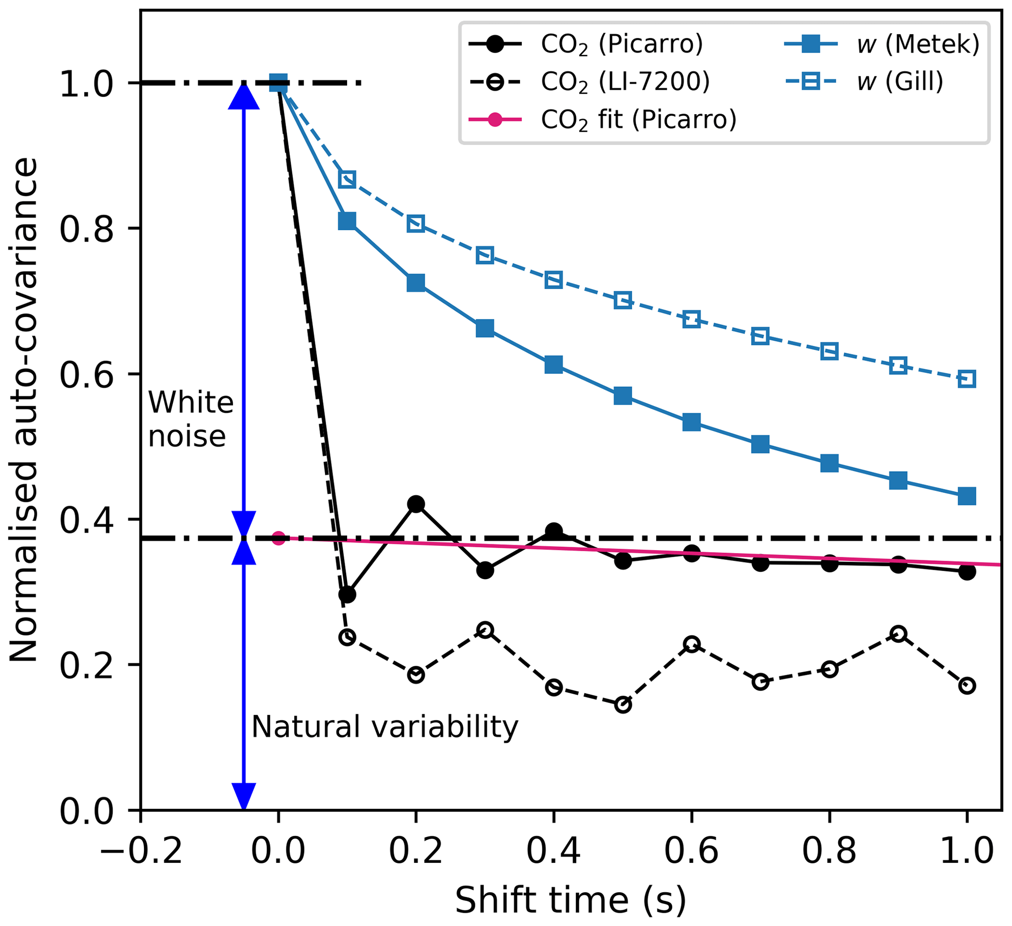
Figure 3 Mean normalised auto-covariance functions of CO₂ and vertical wind velocity (w) by four different instruments. The magenta line represents a fit to the noise-free auto-covariance function of CO₂ (measured by Picarro) extrapolated back to a zero time shift. An example of the white noise and natural variability contributions to the total CO₂ (measured by Picarro) variance is indicated by two blue arrows. The sharp decrease of the CO₂ auto-covariance between the zero shift and the initial 0.1 s shift corresponds to the large contribution of white noise from the gas analysers. The LI-7200 is the noisier instrument. The noise contributions from the anemometer are relatively small (< 10 %).

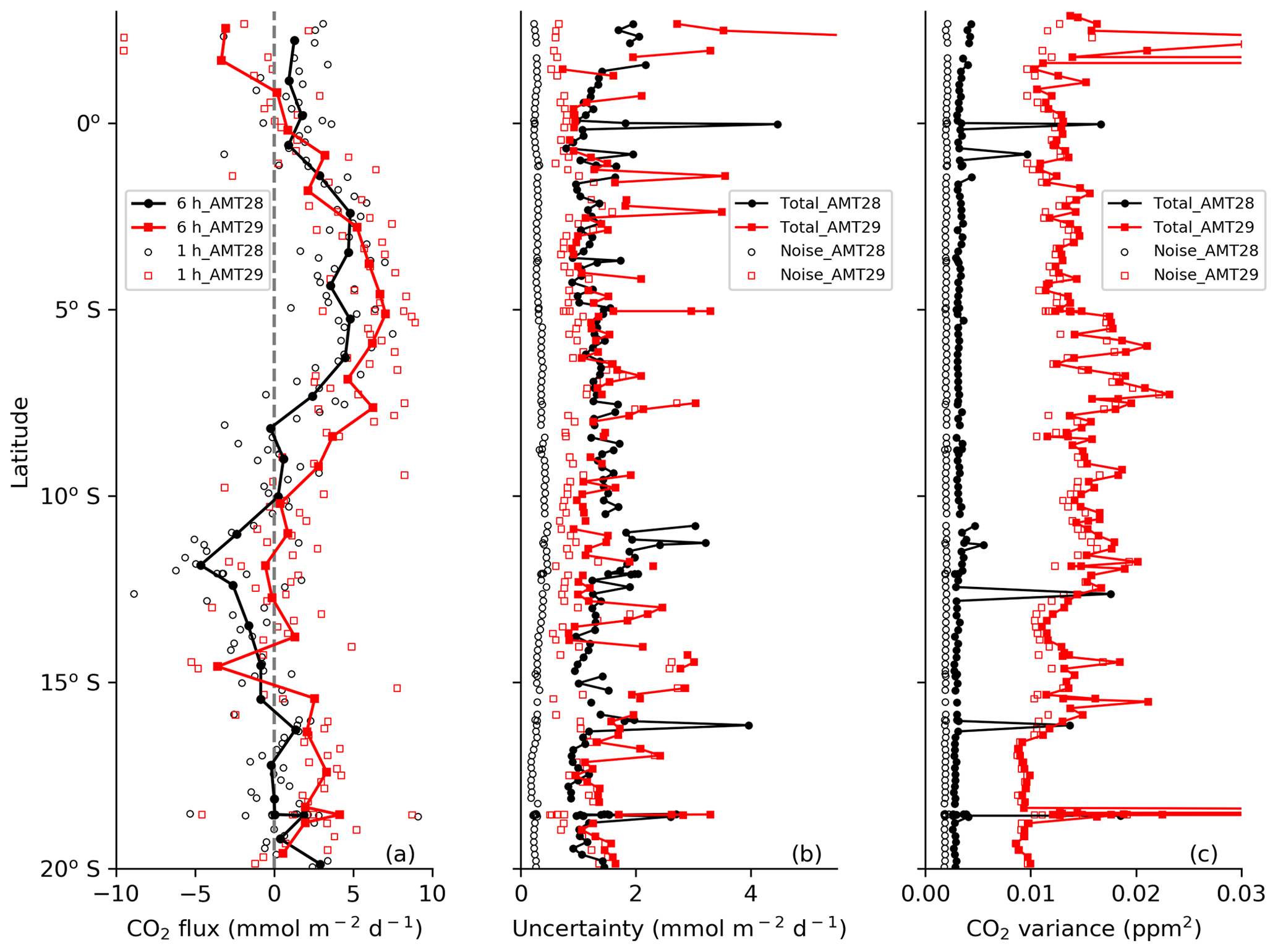
Figure 4 (a) Air–sea CO₂ fluxes (hourly and 6 h averages), (b) random uncertainty in flux (total and due to instrument noise only), and (c) variance in CO₂ mixing ratio (total and due to instrument noise only) for two Atlantic cruises.

3 Results

Measurements from AMT28 and AMT29 set the scene for our uncertainty analysis. These two Atlantic cruises transited across the same tropical region (Fig. A2, Appendix A) in October 2018 and September 2019 with different eddy covariance systems (Sect. 2.1). AMT28 and AMT29 show broadly similar latitudinal patterns (Fig. 4a). An obvious question of interest is whether the measured fluxes were the same for the 2 years. To answer this question, the measurement uncertainties must be quantified. The total random uncertainties in CO₂ flux (δF_{R,Finkelstein}) are comparable for the two cruises, even though the random error component due to instrument noise (δF_RN,Mauder) is about 3 times higher during AMT29 using LI-7200 than during AMT28 using Picarro G2311-f (Fig. 4b; Fig. D1, Appendix D). The similar total random uncertainty in the AMT28 and AMT29 fluxes shows that both gas analysers are equally suitable for air–sea EC CO₂ flux measurements. The variance budgets of atmospheric CO₂ mixing ratio (used to estimate random flux uncertainty; see Sect. 3.1) are shown in Fig. 4c. Total variance in CO₂ mixing ratio is dominated by instrument noise on both cruises. CO₂ mixing ratio variance (total and instrument noise) was substantially higher during AMT29.

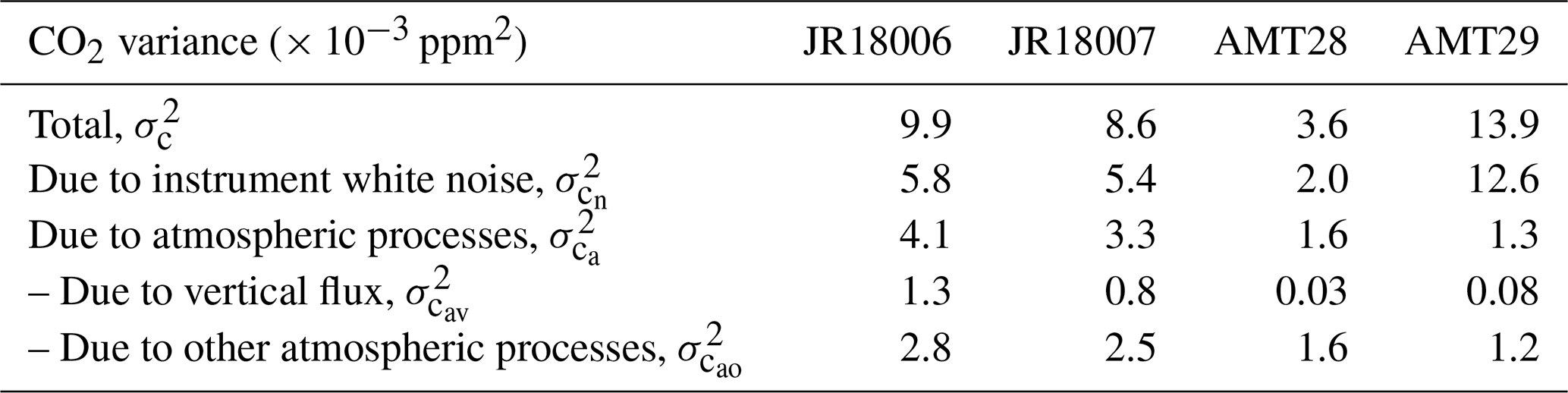
Table 3 Variance in the CO₂ mixing ratio estimated using Eqs. (8) and (11) for the Arctic (JR18006/7, Picarro G2311-f) and Atlantic cruises (AMT28, Picarro G2311-f; AMT29, LI-7200). Total CO₂ variance (${\mathit{\sigma }}_{\mathrm{c}}^{\mathrm{2}}$) consists of white noise (${\mathit{\sigma }}_{{\mathrm{c}}_{\mathrm{n}}}^{\mathrm{2}}$) and atmospheric processes (${\mathit{\sigma }}_{{\mathrm{c}}_{\mathrm{a}}}^{\mathrm{2}}$). The latter can be further broken down to the CO₂ variance due to vertical flux (${\mathit{\sigma }}_{{\mathrm{c}}_{\mathrm{av}}}^{\mathrm{2}}$) and due to other processes (${\mathit{\sigma }}_{{\mathrm{c}}_{\mathrm{ao}}}^{\mathrm{2}}$).

3.1 Random uncertainty

Theoretical derivation of flux uncertainty (δF_RN,Blomquist, Eq. 7) requires knowledge of the contributions to CO₂ mixing ratio variance. Total CO₂ variance is made up of instrument noise (${\mathit{\sigma }}_{{\mathrm{c}}_{\mathrm{n}}}^{\mathrm{2}}$) and atmospheric processes (${\mathit{\sigma }}_{{\mathrm{c}}_{\mathrm{a}}}^{\mathrm{2}}$). Atmospheric processes include vertical flux (${\mathit{\sigma }}_{{\mathrm{c}}_{\mathrm{av}}}^{\mathrm{2}}$) and other atmospheric processes (${\mathit{\sigma }}_{{\mathrm{c}}_{\mathrm{ao}}}^{\mathrm{2}}$). The variance budgets of CO₂ mixing ratio for the four cruises are listed in Table 3. Atmospheric processes contribute a larger CO₂ variance in the Arctic (where flux magnitudes are greater) compared to the Atlantic. Vertical flux accounts for ∼ 10 % of the variance in CO₂ mixing ratio in the Arctic and ∼ 1 % of the CO₂ variance in the Atlantic. Previous results demonstrate that horizontal transport is a major source of ${\mathit{\sigma }}_{{\mathrm{c}}_{\mathrm{ao}}}^{\mathrm{2}}$ for long-lived greenhouse gases (Blomquist et al., 2012). Small changes in CO₂ mixing ratio transported horizontally can yield variance that greatly exceeds the variance from vertical flux.

Three quasi-independent methods were used to estimate random uncertainty in EC air–sea CO₂ fluxes caused by instrument noise (δF_RN; Methods C–E, Sect. 2.3.3). Good agreement was found between all three estimates (Fig. C2, Appendix C) when $\sqrt{\mathrm{2}}$ is used as the constant in Eq. (7) (a). The ΔF_{RN,Billesbach} estimates have more scatter and are slightly higher than the theoretical results, possibly because the random shuffling of data fails to fully exclude the contribution from atmospheric turbulence (Rannik et al., 2016). For the remainder of this study, we use the δF_RN,Mauder method to estimate δF_RN.

We used three methods to estimate the total random uncertainty (δF_R; Methods A–C, Sect. 2.3.3) in the hourly averaged air–sea CO₂ fluxes. There is good agreement among the three estimates (r > 0.88; Fig. C1, Appendix C). Again, the constant in Eq. (7) (a) is set to $\sqrt{\mathrm{2}}$, as informed by the instrument noise uncertainty analysis above. We use δF_{R,Finkelstein} (Eq. 6) to estimate the total random flux uncertainty hereafter. Our decision is based on δF_{R,Finkelstein} not requiring the integral timescale (unlike δF_R,Blomquist) and showing less scatter than δF_R,Wienhold.

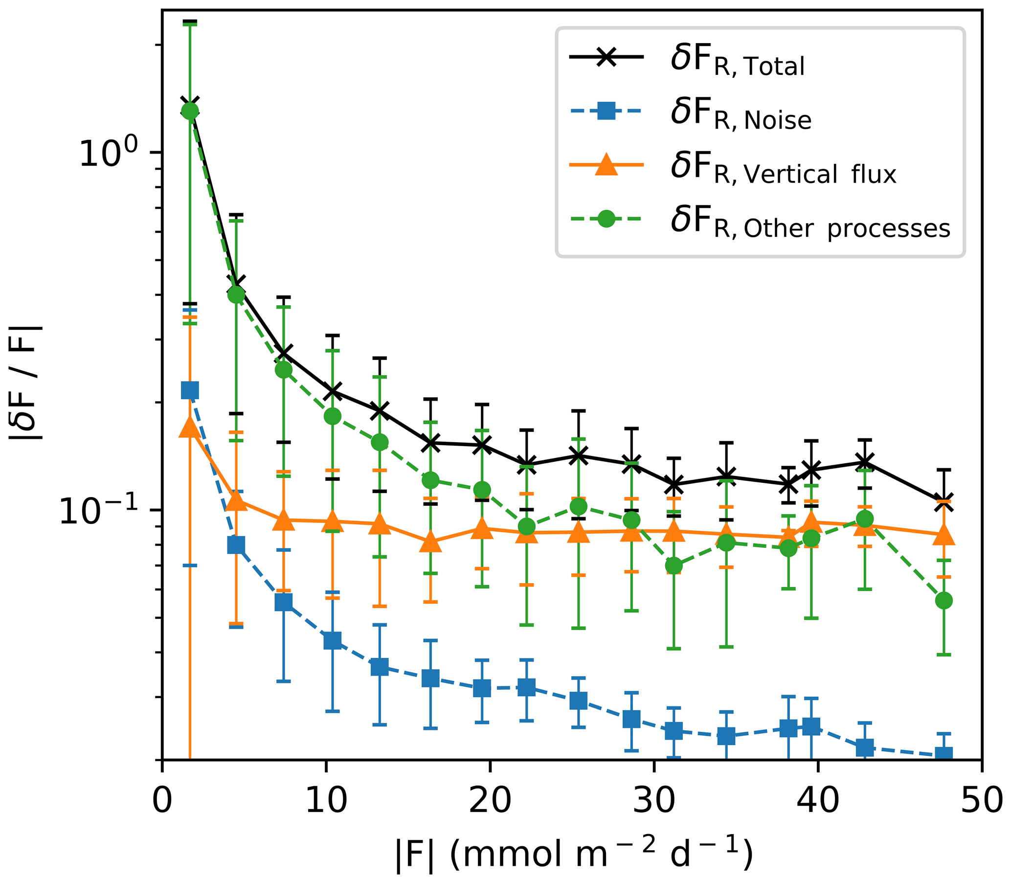
Figure 5 Relative random uncertainty in hourly CO₂ flux and its contribution from noise, vertical flux, and other processes during two Arctic cruises. Relative random uncertainty data are binned into 3 $\mathrm{mmol}{\mathrm{m}}^{-\mathrm{2}}{\mathrm{d}}^{-\mathrm{1}}$ flux magnitude bins (error bars represent 1 standard deviation).

Figure 5 shows the different relative contributions to the random flux uncertainty for the Arctic cruises (hourly average). Here the uncertainty is normalised by the flux magnitude and then averaged into flux magnitude bins. When the flux magnitude is sufficiently large (> 20 $\mathrm{mmol}{\mathrm{m}}^{-\mathrm{2}}{\mathrm{d}}^{-\mathrm{1}}$), the total relative random uncertainty in flux asymptotes to about 15 % and is driven by variance associated with both vertical flux and other atmospheric processes. This estimate is similar to uncertainties in air–sea fluxes of other well resolved (i.e. high signal-to-noise ratio) variables (Fairall et al., 2000). At a lower flux magnitude, uncertainty due to atmospheric processes other than vertical flux dominates the total random uncertainty. Uncertainty due to the white noise from the Picarro G2311-f gas analyser is small.

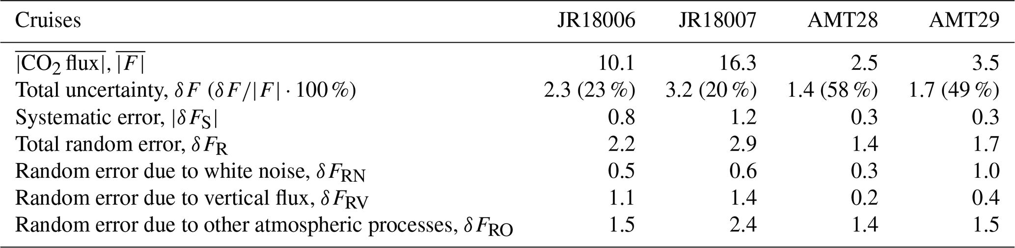
Table 4 Summary of hourly average EC CO₂ fluxes and associated uncertainties in the mean for the four cruises ($\mathrm{mmol}{\mathrm{m}}^{-\mathrm{2}}{\mathrm{d}}^{-\mathrm{1}}$). Shown are the mean CO₂ flux magnitude ($\stackrel{\mathrm{‾}}{\mathrm{|}F\mathrm{|}}$, $\mathrm{mmol}{\mathrm{m}}^{-\mathrm{2}}{\mathrm{d}}^{-\mathrm{1}}$), upper limitation of the total uncertainty (δF; Eq. 3), upper limitation of the absolute systematic error (|δF_S|; propagated from Table 2 and Eq. 5), and random error (δF_R; Eq. 6). The random error components are white noise (δF_RN; Eq. 10), vertical flux (δF_RV; Eqs. 7 and 8), and other atmospheric processes ($\mathit{\delta }{F}_{\text{RO}}=\sqrt{\mathit{\delta }{F}_{\mathrm{R}}^{\mathrm{2}}-\mathit{\delta }{F}_{\text{RN}}^{\mathrm{2}}-\mathit{\delta }{F}_{\text{RV}}^{\mathrm{2}}}$). The total uncertainty is also expressed as a percentage of the mean flux magnitude ($\mathit{\delta }F/\mathrm{|}F\mathrm{|}\cdot \mathrm{100}\mathit{\%}$).

3.2 Summary of systematic and random uncertainties

The total uncertainty δF in the hourly average EC CO₂ flux (estimated using Eq. 3) ranges from 1.4 to 3.2 $\mathrm{mmol}{\mathrm{m}}^{-\mathrm{2}}{\mathrm{d}}^{-\mathrm{1}}$ in the mean for the four cruises (Table 4). Our EC flux system setup was optimal, and subsequent corrections have minimised any bias to < 9 % (Sect. 2.3.2). Systematic error is on average much lower than random error (Table 4). This means the accuracy of the EC CO₂ flux measurements is very high, but the precision of hourly averaged EC CO₂ air–sea flux measurements is relatively low. In Sect. 4.1, we discuss how the precision can be improved by averaging the observed fluxes for longer.

The theoretical uncertainty estimates above can be compared with a portion of the AMT28 cruise data (15–20^∘ S, ∼ 25^∘ W; Fig. 4), when the ship encountered sea surface CO₂ fugacity close to equilibrium with the atmosphere (i.e. ΔfCO₂ ∼ 0; Fig. A2, Appendix A). The data from this region are useful for assessing the random and systematic flux uncertainties. The standard deviation of the EC CO₂ flux during cruise AMT28 when ΔfCO₂ ∼ 0 is 1.6 $\mathrm{mmol}{\mathrm{m}}^{-\mathrm{2}}{\mathrm{d}}^{-\mathrm{1}}$, which compares well with the theoretical random flux uncertainty in this region (1.4 $\mathrm{mmol}{\mathrm{m}}^{-\mathrm{2}}{\mathrm{d}}^{-\mathrm{1}}$). The mean EC CO₂ flux from this region was 0.5 $\mathrm{mmol}{\mathrm{m}}^{-\mathrm{2}}{\mathrm{d}}^{-\mathrm{1}}$, which is indistinguishable from zero considering the random uncertainty. This further confirms the minimal bias in our flux observations.

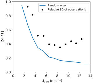
Figure 6 Comparison of relative random uncertainty in hourly CO₂ flux and relative standard deviation (RSTD; $\text{standard\hspace{0.17em} deviation}/\mathrm{|}\text{flux\hspace{0.17em} mean}\mathrm{|}$) of the EC CO₂ flux from two Arctic cruises. These results are binned in 1 m s⁻¹ wind speed bins.

Figure 6 shows a comparison between the relative uncertainty and the relative standard deviation (RSTD) in the hourly CO₂ flux for the two Arctic cruises. Results have been binned into 1 m s⁻¹ wind speed bins. Wind speed was converted to 10 m neutral wind speed (U_10N) using the COARE3.5 model (Edson et al., 2013). The relative random error decreases with increasing wind speed. This is partly because the fluxes tend to be larger at higher wind speeds, and so the signal-to-noise ratio in the flux is greater. In addition, at higher wind speeds, a greater number of high-frequency turbulent eddies are sampled by the EC system, providing better statistics of turbulent eddies and lower sampling error.

The RSTD of the flux is greater in magnitude than the estimated flux uncertainty because it also contains environmental variability. The CO₂ flux auto-covariance analysis (Sect. 4.1) shows that random error in hourly flux explains ∼ 20 % of the flux variance on average for the two Arctic cruises. This implies that the remaining variability in the EC flux (∼ 80 %) is due to natural phenomena (e.g. changes in ΔfCO₂ or wind speed). Similarly, substantial variability is typical in EC-derived CO₂ gas transfer velocity at a given wind speed (e.g. Edson et al., 2011; Butterworth and Miller, 2016). K₆₆₀ is derived from $\left(\text{EC}{\mathrm{CO}}_{\mathrm{2}}\text{flux}\right)/\mathrm{\Delta }f{\mathrm{CO}}_{\mathrm{2}}$, and thus an understanding of EC flux uncertainty can help understand and explain the variability in EC-derived gas transfer velocity estimates (Sect. 4.2).

4 Discussion

4.1 Impact of averaging timescale on flux uncertainty

The random error in flux decreases with increasing averaging time interval T or the number of sampling points n (Eqs. 6, 7, and 10). This is because a longer averaging time interval results in better statistics of the turbulent eddies. However, averaging for too long is also not ideal since the atmosphere is less likely to maintain stationarity. The typical averaging time interval is thus typically between 10 min and 60 min for air–sea flux measurements (20 min intervals were used in this study). The time series of quality controlled 20 min flux intervals can be further averaged over a longer timescale to reduce the random uncertainty. Averaging the 20 min flux intervals assumes that the flux interval data are essentially repeat measurements within a chosen averaging timescale. If the 20 min flux intervals are averaged, one can ask the following question: what is the optimal averaging timescale for interpreting air–sea EC CO₂ fluxes?

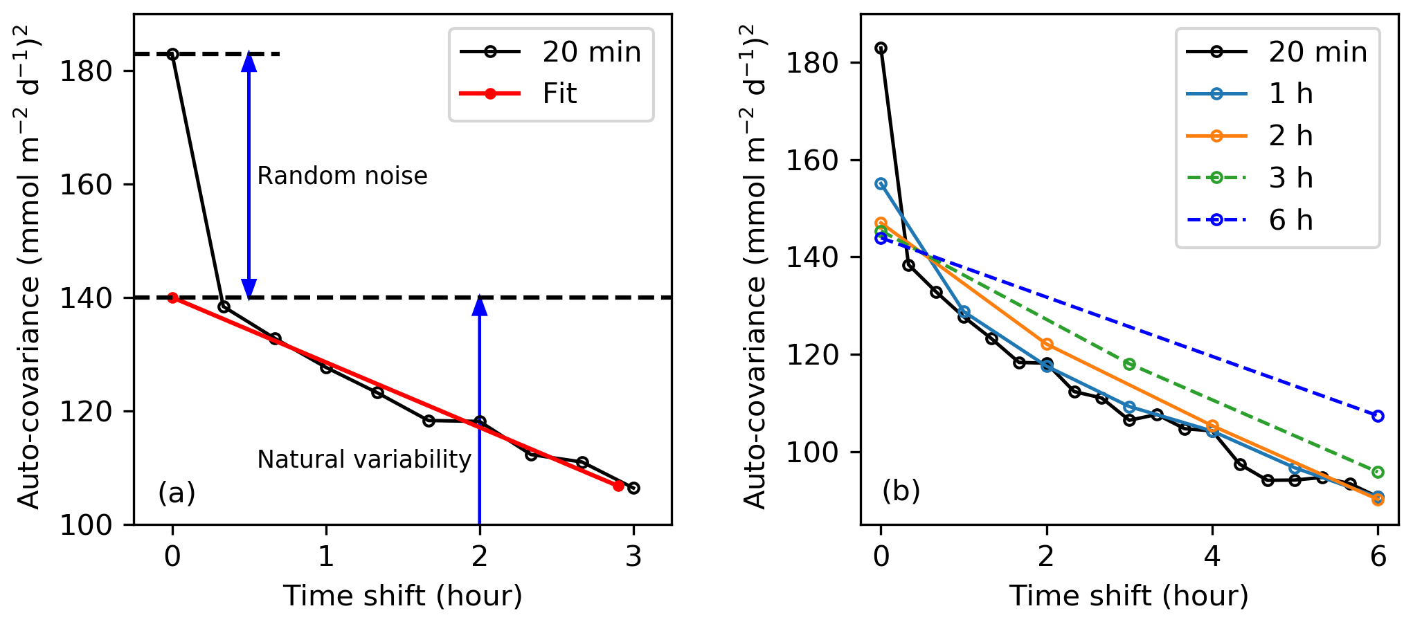
Figure 7 (a) Auto-covariance of the original 20 min fluxes (cruise JR18007) and a fit to the noise-free auto-covariance function extrapolated back to a zero time shift. (b) CO₂ flux auto-covariance functions with different averaging timescales. The black line represents the auto-covariance of the original 20 min fluxes. The 20 min fluxes are further averaged at different timescales (1, 2, 3, and 6 h), and the corresponding auto-covariance functions are shown with different colours (dark blue, orange, green, and light blue).

We use an auto-covariance method to determine the optimal averaging timescale. The observed variance in CO₂ flux consists of random uncertainty (random noise) as well as natural variability. The random noise component should only contribute to the CO₂ flux variance when the data are zero-shifted. After the CO₂ flux data are shifted, the noise will not contribute to the auto-covariance function. Figure 7 shows the auto-covariance function of the air–sea CO₂ flux with different averaging timescales for Arctic cruise JR18007. For the 20 min fluxes (Fig. 7a), the auto-covariance decreases rapidly between the zero shift and the initial time shift, which indicates that a large fraction of the 20 min flux variance is due to random noise.

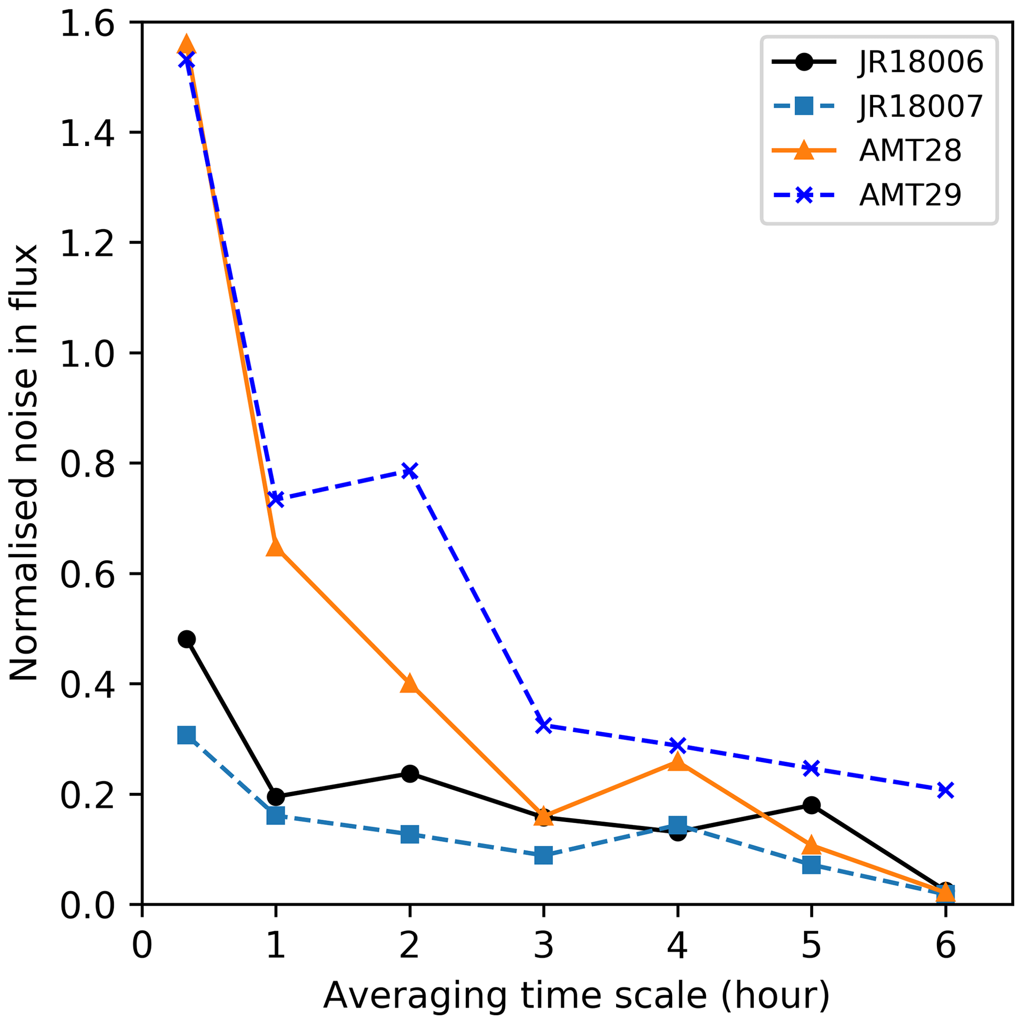
Figure 8 Effect of the averaging timescale on the noise:signal ($\text{random\hspace{0.17em} noise\hspace{0.17em} in\hspace{0.17em} flux}/\text{natural\hspace{0.17em} flux\hspace{0.17em} variability}$) for EC air–sea CO₂ flux measurements during four cruises.

The random noise in the CO₂ fluxes decreases with a longer averaging timescale, with the greatest effect observed from 20 min to 1 h (Fig. 7b). A fit to the noise-free auto-covariance function extrapolated back to a zero time shift gives us an estimate of the non-noise variability in the natural CO₂ flux. Subtracting the extrapolated natural flux variability from the total variance in CO₂ flux provides an estimate of the random noise in the flux for each averaging timescale (Fig. 7a). All four cruises consistently demonstrate a non-linear reduction in the noise contribution to the flux measurements when the averaging timescale increases (Fig. 8). The random noise in flux can be expressed relative to the natural variance in flux representing the inverse of the signal-to-noise ratio (i.e. $\text{random\hspace{0.17em} noise\hspace{0.17em} in\hspace{0.17em} flux}/\text{natural\hspace{0.17em} flux\hspace{0.17em} variability}$, hereafter referred to as noise:signal).

The noise:signal also facilitates comparison of all four cruises (Fig. 8) and demonstrates the consistent effect that increasing the averaging timescale has on noise:signal. Consistent with Table 4, the Arctic cruises show much lower noise:signal because the flux magnitudes are much larger. Typical detection limits in analytical science are often defined by a 1:3 noise:signal ratio. A 1:3 noise:signal is achieved with a 1 h averaging timescale for the Arctic cruises. The Atlantic cruises encountered much lower air–sea CO₂ fluxes, and an averaging timescale of at least 3 h is required to achieve the same 1:3 noise:signal ratio.

The flux measurement uncertainty at a 6 h averaging timescale for the AMT cruises is ∼ 0.6 $\mathrm{mmol}{\mathrm{m}}^{-\mathrm{2}}{\mathrm{d}}^{-\mathrm{1}}$. The analysis presented above permits an answer to the question posed at the beginning of the Results section. The mean difference between the 6 h averaged EC CO₂ flux observations on AMT29 and AMT28 (1.3 $\mathrm{mmol}{\mathrm{m}}^{-\mathrm{2}}{\mathrm{d}}^{-\mathrm{1}}$; Fig. 4a) is much greater than the measurement uncertainty. This significant difference was likely because of the interannual variability in AMT CO₂ flux due to changes in the natural environment (e.g. ΔfCO₂, sea surface temperature, and physical drivers of interfacial turbulence such as wind speed) during the two cruises.

At a typical research ship speed of ∼ 10 knots, the AMT cruises cover ∼ 110 km in 6 h, which is equivalent to ∼ 1^∘ latitude. Averaging for longer than 6 h is likely to cause substantial loss of real information about the natural variations in air–sea CO₂ flux and the drivers of flux variability. For example, the mean flux between 0–20^∘ S during cruise AMT28 is 0.9 $\mathrm{mmol}{\mathrm{m}}^{-\mathrm{2}}{\mathrm{d}}^{-\mathrm{1}}$. However, the 6 h average EC measurements show that the flux varied between +5 $\mathrm{mmol}{\mathrm{m}}^{-\mathrm{2}}{\mathrm{d}}^{-\mathrm{1}}$ (∼ 2–6^∘ S) and −5 $\mathrm{mmol}{\mathrm{m}}^{-\mathrm{2}}{\mathrm{d}}^{-\mathrm{1}}$ (∼ 11–13^∘ S; Fig. 4a).

4.2 Effect of CO₂ flux uncertainty on the gas transfer velocity K

The uncertainties in the EC CO₂ air–sea flux measurement will influence the uncertainty that translates to EC-based estimates of the gas transfer velocity, K. For illustration, K is computed for Arctic cruise JR18007, which had a high flux signal:noise ratio of ∼ 5 (Fig. 8). Any data potentially influenced by ice and sea ice melt were excluded using a sea surface salinity filter (data excluded when salinity < 32). Equation (1) is rearranged and used with concurrent measurements of CO₂ flux (F), ΔfCO₂, and sea surface temperature (SST) to obtain K adjusted for the effect of temperature (K₆₆₀).

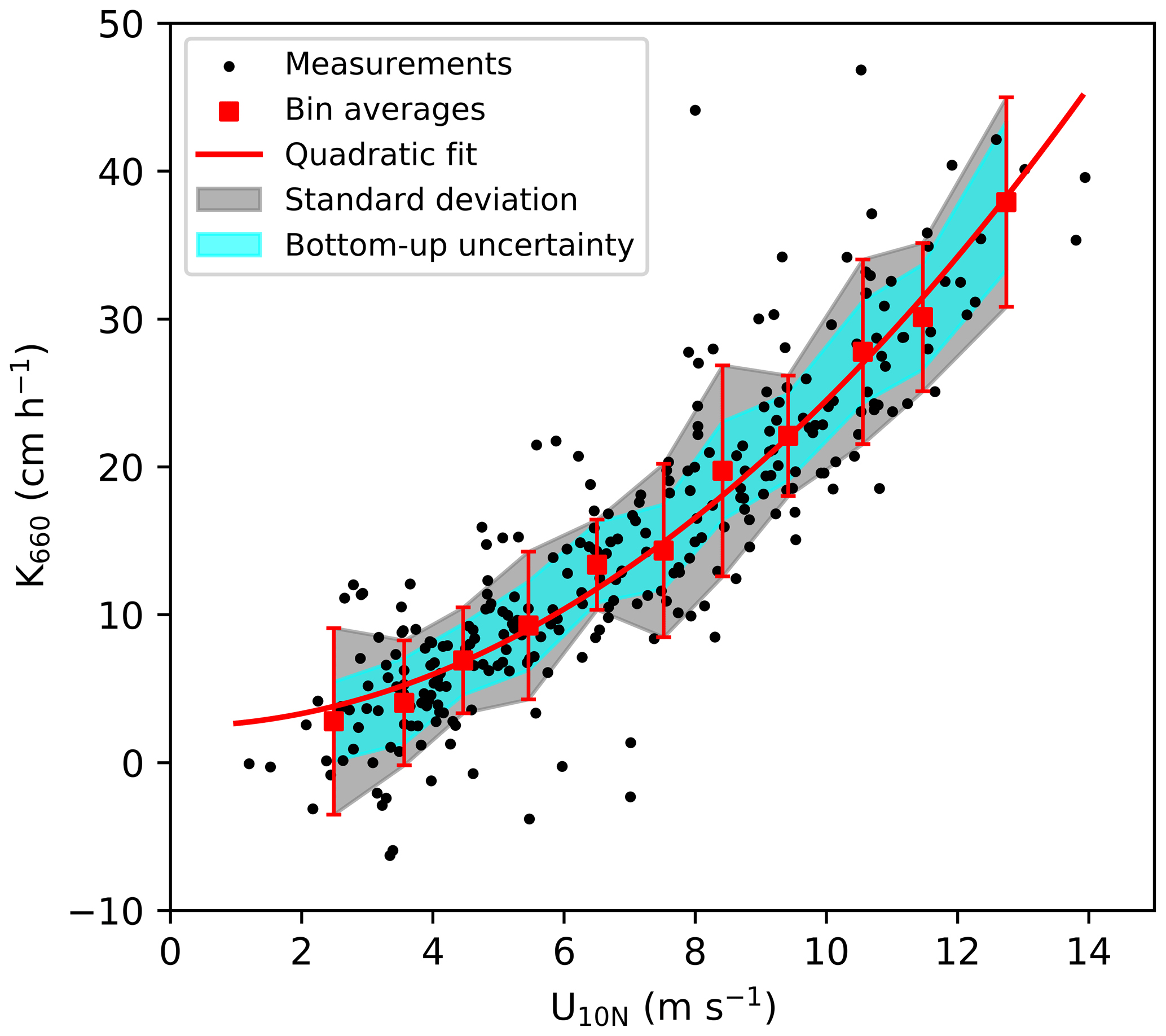
Figure 9 Gas transfer velocity (K₆₆₀) measured on Arctic cruise JR18007 (hourly average, signal:noise ∼ 5) vs. 10 m neutral wind speed (U_10N). Red squares represent 1 m s⁻¹ bin averages, with error bars representing 1 standard deviation (SD). The red curve represents a quadratic fit using the bin averages: K₆₆₀ = 0.22 $U_{\mathrm{10}\mathrm{N}}^{\mathrm{2}}$ + 2.46 (R² = 0.76). The grey shaded area represents the standard deviation calculated for each wind speed bin (K₆₆₀ ± 1 SD). The cyan region represents the upper and lower bounds in K₆₆₀ uncertainty computed from the EC flux uncertainty (K₆₆₀ ± δK₆₆₀; see text for detail).

The determination coefficient (R²) of the quadratic fit between wind speed (U_10N) and EC-derived K₆₆₀ (Fig. 9) demonstrates that wind speed explains 76 % of the K₆₆₀ variance during Arctic cruise JR18007. How much of the remaining 24 % can be attributed to uncertainties in EC CO₂ fluxes?

Variability in K₆₆₀ within each 1 m s⁻¹ wind speed bin can be considered to have minimal wind speed influence. It is thus useful to compare the variability within each wind speed bin (K₆₆₀ ± 1 SD) with the upper and lower uncertainty bounds derived from the EC flux measurements. Uncertainty in EC flux-derived K₆₆₀ (δK₆₆₀) is calculated from the uncertainty in hourly EC flux (δF) by rearranging Eq. (1) (bulk flux equation) and replacing F with δF. The resultant δK₆₆₀ is then averaged in wind speed bins. The shaded cyan band in Fig. 9 (K₆₆₀ ± δK₆₆₀) is consistently narrower than the grey shaded band (K₆₆₀ ± 1 SD). On average, EC flux-derived uncertainty in K₆₆₀ can only account for a quarter of the K₆₆₀ variance within each wind speed bin, and the remaining variance is most likely due to the non-wind speed factors that influence gas exchange (e.g. breaking waves, surfactants).

The analysis above can be extended to assess how EC flux-derived uncertainty affects our ability to parameterise K₆₆₀ (e.g. as a function of wind speed). To do so, a set of synthetic K₆₆₀ data is generated (same U_10N as the K₆₆₀ measurements in Fig. 9). The synthetic K₆₆₀ data are initialised using a quadratic wind speed dependence that matches JR18007 (i.e. K₆₆₀ = 0.22 $U_{\mathrm{10}\mathrm{N}}^{\mathrm{2}}$ + 2.46). Random Gaussian noise is then added to the synthetic K₆₆₀ data, with relative noise level corresponding to the relative flux uncertainty values taken from JR18007 (mean of 20 %; Table 4). The relative uncertainty in K₆₆₀ due to EC flux uncertainty ($\mathit{\delta }{K}_{\mathrm{660}}/K_{\mathrm{660}}$) shows a wind speed dependence (Fig. S4a in the Supplement), and the artificially generated Gaussian noise incorporates this wind speed dependence (Fig. S4b, Supplement). The R² of the quadratic fit to the synthetic data as a function of U_10N is 0.90 (the rest of the variance is due to uncertainty in K₆₆₀). Since wind speed explains 76 % of variance in the observed K₆₆₀, it can be inferred that non-wind speed factors can account for 14 % (i.e. (100–76) %–(100–90) %) of the total variance in K₆₆₀ from this Arctic cruise. If the synthetic K₆₆₀ data are assigned a relative flux uncertainty of 50 % (reflective of a region with low fluxes, e.g. AMT28/29), the R² of the wind speed dependence in the synthetic data decreases to 0.60.

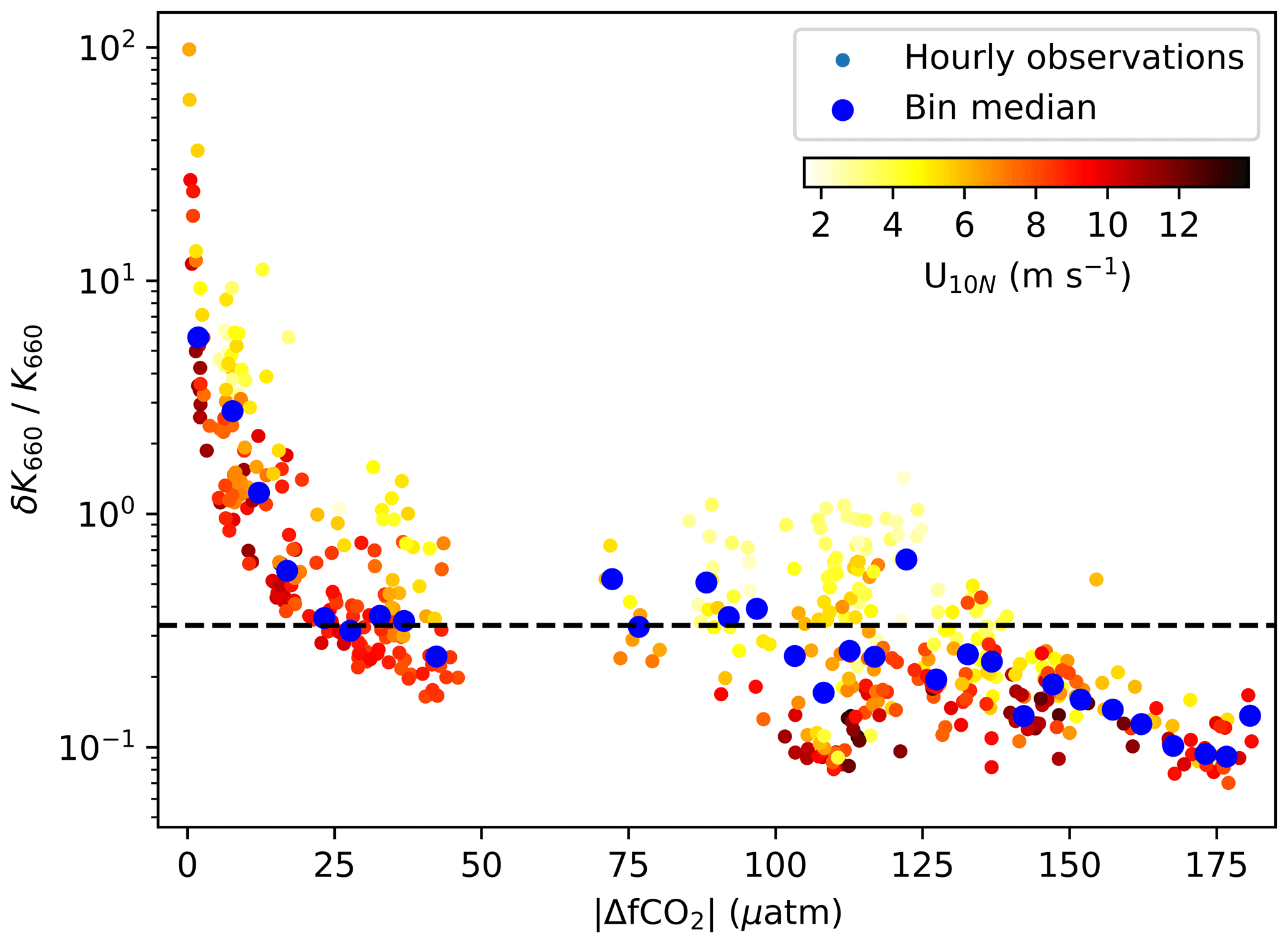
Figure 10 Relative uncertainty in EC-estimated hourly K₆₆₀ ($\mathit{\delta }{K}_{\mathrm{660}}/K_{\mathrm{660}}$) vs. the magnitude of the air–sea CO₂ fugacity difference (|ΔfCO₂|) during Arctic cruise JR18007 and Atlantic cruises AMT28 and AMT29 (no ΔfCO₂ data were collected on JR18006). The data points are colour-coded by wind speed. Blue points are medians of $\mathit{\delta }{K}_{\mathrm{660}}/K_{\mathrm{660}}$ in 5 µatm bins. Here we use the parameterised K₆₆₀ (= 0.22 $U_{\mathrm{10}\mathrm{N}}^{\mathrm{2}}$ + 2.46) to normalise the uncertainty in K₆₆₀. The dashed line represents the 3:1 signal:noise ratio ($\mathit{\delta }{K}_{\mathrm{660}}/K_{\mathrm{660}}=\mathrm{1}/\mathrm{3})$.

The relative uncertainty in EC flux-derived K₆₆₀ ($\mathit{\delta }{K}_{\mathrm{660}}/K_{\mathrm{660}}$) is large when |ΔfCO₂| is small (Fig. 10). Previous EC studies have filtered EC flux data to remove fluxes when the |ΔfCO₂| falls below a specified threshold (e.g. 20 µatm, Blomquist et al. (2017); 40 µatm, Miller et al. (2010), Landwehr et al. (2014), Butterworth and Miller (2016), Prytherch et al. (2017); 50 µatm, Landwehr et al. (2018)). Analysis of the data presented here suggests that a |ΔfCO₂| threshold of at least 20 µatm is reasonable for hourly K₆₆₀ measurements, leading to δK₆₆₀ of ∼ 10 cm h⁻¹ ($\mathit{\delta }{K}_{\mathrm{660}}/K_{\mathrm{660}}$ ∼ $\mathrm{1}/\mathrm{3}$) or less on average. At very large |ΔfCO₂| of over 100 µatm, δK₆₆₀ is reduced to only a few centimetres per hour (cm h⁻¹) ($\mathit{\delta }{K}_{\mathrm{660}}/K_{\mathrm{660}}$ ∼ 1/5). At longer flux averaging timescales, it may be possible to relax the minimal |ΔfCO₂| threshold.

5 Conclusions

This study uses data from four cruises with a range in air–sea CO₂ flux magnitude to comprehensively assess the sources of uncertainty in EC air–sea CO₂ flux measurements. Data from two ships and two different state-of-the-art CO₂ analysers (Picarro G2311-f and LI-7200, both fitted with a dryer) are analysed using multiple methods (Sect. 2.3). Random error accounts for the majority of the flux uncertainty, while the systematic error (bias) is small (Table 4). Random flux uncertainty is primarily caused by variance in CO₂ mixing ratio due to atmospheric processes. The random error due to instrument noise for the Picarro G2311-f is 3-fold smaller than for LI-7200 (Table 4 and Fig. D1, Appendix D). However, the contribution of the instrument noise to the total random uncertainty is much smaller than the contribution of atmospheric processes such that both gas analysers are well suited for air–sea CO₂ flux measurements.

The mean uncertainty in hourly EC flux is estimated to be 1.4–3.2 $\mathrm{mmol}{\mathrm{m}}^{-\mathrm{2}}{\mathrm{d}}^{-\mathrm{1}}$, which equates to the relative uncertainty of ∼ 20 % in high CO₂ flux regions and ∼ 50 % in low CO₂ flux regions. Lengthening the averaging timescale can improve the signal:noise ratio in EC CO₂ flux through the reduction of random uncertainty. Auto-covariance analysis of CO₂ flux is used to quantify the optimal averaging timescale (Figs. 7 and 8, Sect. 4.1). The optimal averaging timescale varies between 1 h for regions of large CO₂ flux (Arctic in our analysis) and at least 3 h for regions of low CO₂ flux (tropical/subtropical Atlantic in our analysis).

The measurement uncertainty in EC CO₂ flux contributes directly to scatter in the derived gas transfer velocity, K₆₆₀. Flux uncertainties determined in this paper are applied to a synthetic K₆₆₀ dataset. This enables a partitioning of the variance in measured K₆₆₀ that is due to EC CO₂ flux uncertainty, wind speed, and other processes (10 %, 76 %, 14 % for Arctic cruise JR18007). At a given averaging timescale, a |ΔfCO₂| threshold helps to reduce the scatter in K₆₆₀. A minimum |ΔfCO₂| filter of 20 µatm is needed for interpreting hourly K₆₆₀ data, with the signal:noise ratio in K₆₆₀ improving further at higher |ΔfCO₂|.

Appendix A: Cruise tracks

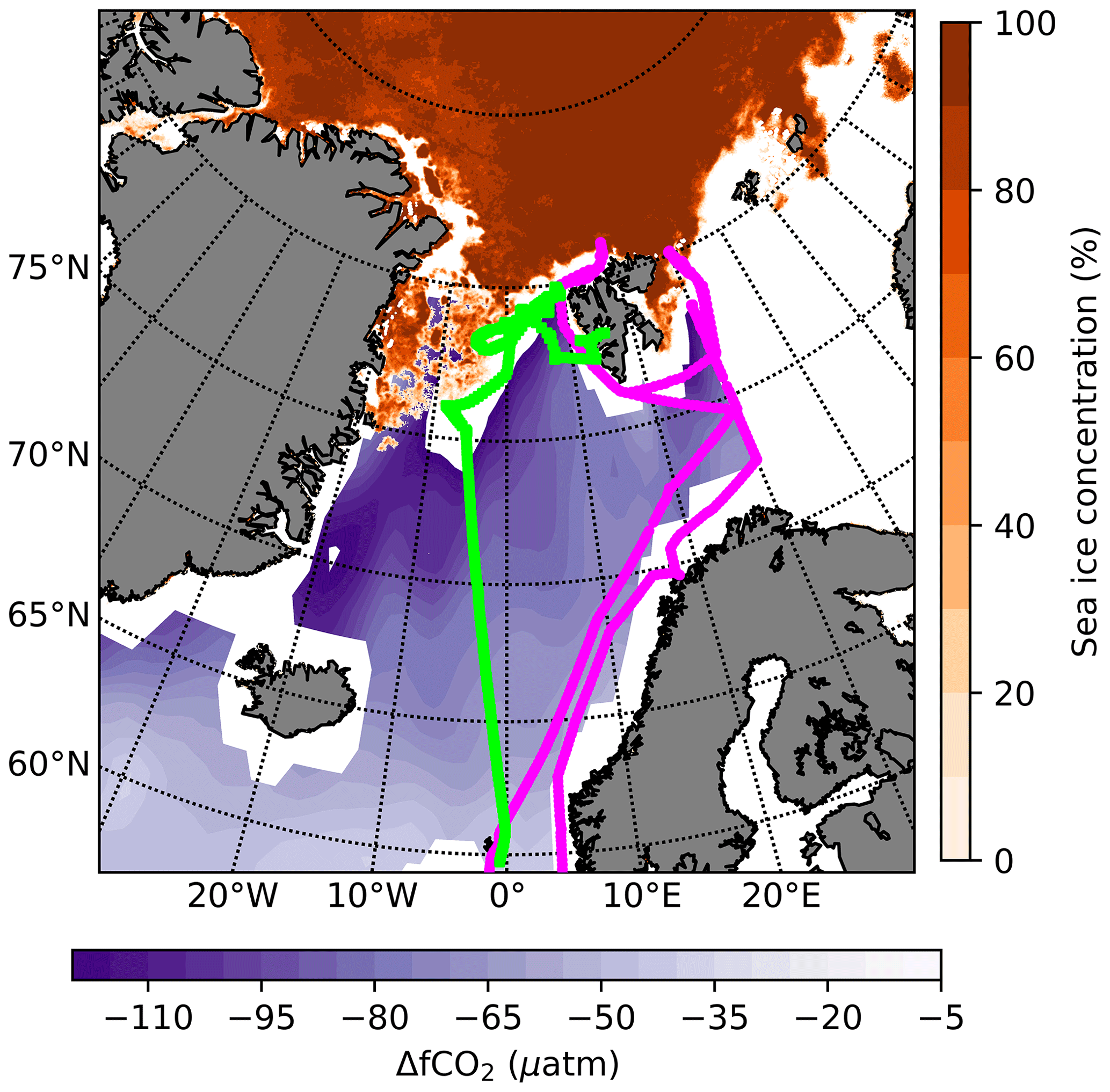
Figure A1 Cruise tracks of JR18006 (magenta) and JR18007 (green). The bottom colour bar indicates the CO₂ fugacity difference (ΔfCO₂) of August 2019 (Bakker et al., 2016; Landschützer et al., 2020), while the right colour bar shows the Arctic sea ice concentrations of 1 August 2019 measured by Advanced Microwave Scanning Radiometer – Earth Observing System Sensor (AMSR-E; Spreen et al., 2008).

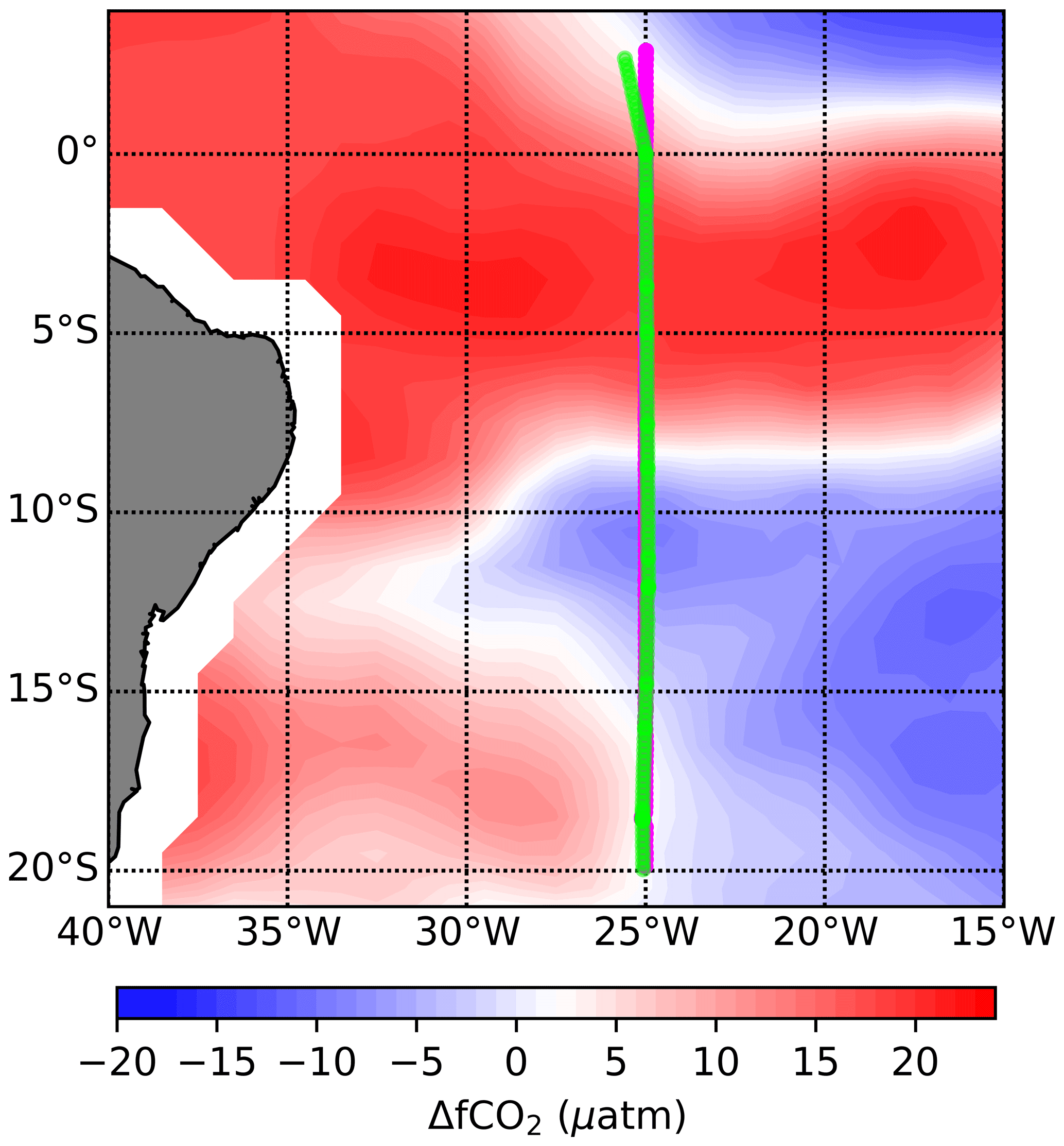
Figure A2 Cruise tracks of AMT28 (magenta) and AMT29 (green). The ocean is coloured with the ΔfCO₂ for October 2018 (Bakker et al., 2016; Landschützer et al., 2020).

Appendix B: Integral timescale and variance spectra of CO₂ and vertical wind velocity

Integral timescale is used in the flux uncertainty calculation (Eqs. 5 and 7). The definition of integral timescale τ_x of variable x is

$$\begin{array}{}\text{(B1)}& {\mathit{\tau }}_x={\displaystyle \frac{\mathrm{1}}{{\mathit{\sigma }}_x^{\mathrm{2}}}}\underset{\mathrm{0}}{\overset{\mathrm{\infty }}{\int }}{r}_{xx}\left(t\right)\mathrm{d}t,\end{array}$$

where ${\mathit{\sigma }}_x^{\mathrm{2}}$ is the variance of x, and r_xx is the auto-covariance function of x. t is the shifting time of auto-covariance (which is different from the lag time between w and CO₂ in the EC flux calculation). We can use Eq. (B1) to estimate the integral timescale of w and CO₂ directly. However, integration up to infinity is not practical. Instead we can numerically estimate the timescale by determining the time corresponding to the auto-covariance coefficient function ($r_{xx}/{\mathit{\sigma }}_x^{\mathrm{2}}$) value decaying to $\mathrm{1}/e$ ($\mathrm{1}/e$ decaying method) or by integrating the auto-covariance function up to the first zero crossing of the function (zero crossing method) (Rannik et al., 2009).

One can also use similarity theory to estimate the integral timescale theoretically (Blomquist et al., 2010):

$$\begin{array}{}\text{(B2)}& {\mathit{\tau }}_{\mathrm{w}}=\mathrm{2.8}{\displaystyle \frac{z}{\stackrel{\mathrm{‾}}{u_{\mathrm{r}}}}}{f}_{\mathit{\tau }}(z/L).\end{array}$$

Here, $\stackrel{\mathrm{‾}}{u_{\mathrm{r}}}$ is the relative wind speed. The similarity function $f_{\mathit{\tau }}(z/L)$ is described by the stability parameter $z/L$, where z is the observation height (m), and L is the Obukhov length (m) (Blomquist et al., 2010).

Yet another method to estimate the integral timescale is from the peak frequency (f_max) in the w variance spectrum (Kaimal and Finnigan, 1994):

$$\begin{array}{}\text{(B3)}& {\mathit{\tau }}_{\mathrm{w}}={\displaystyle \frac{\mathrm{1}}{\mathrm{2}\mathit{\pi }{f}_{max}}}.\end{array}$$

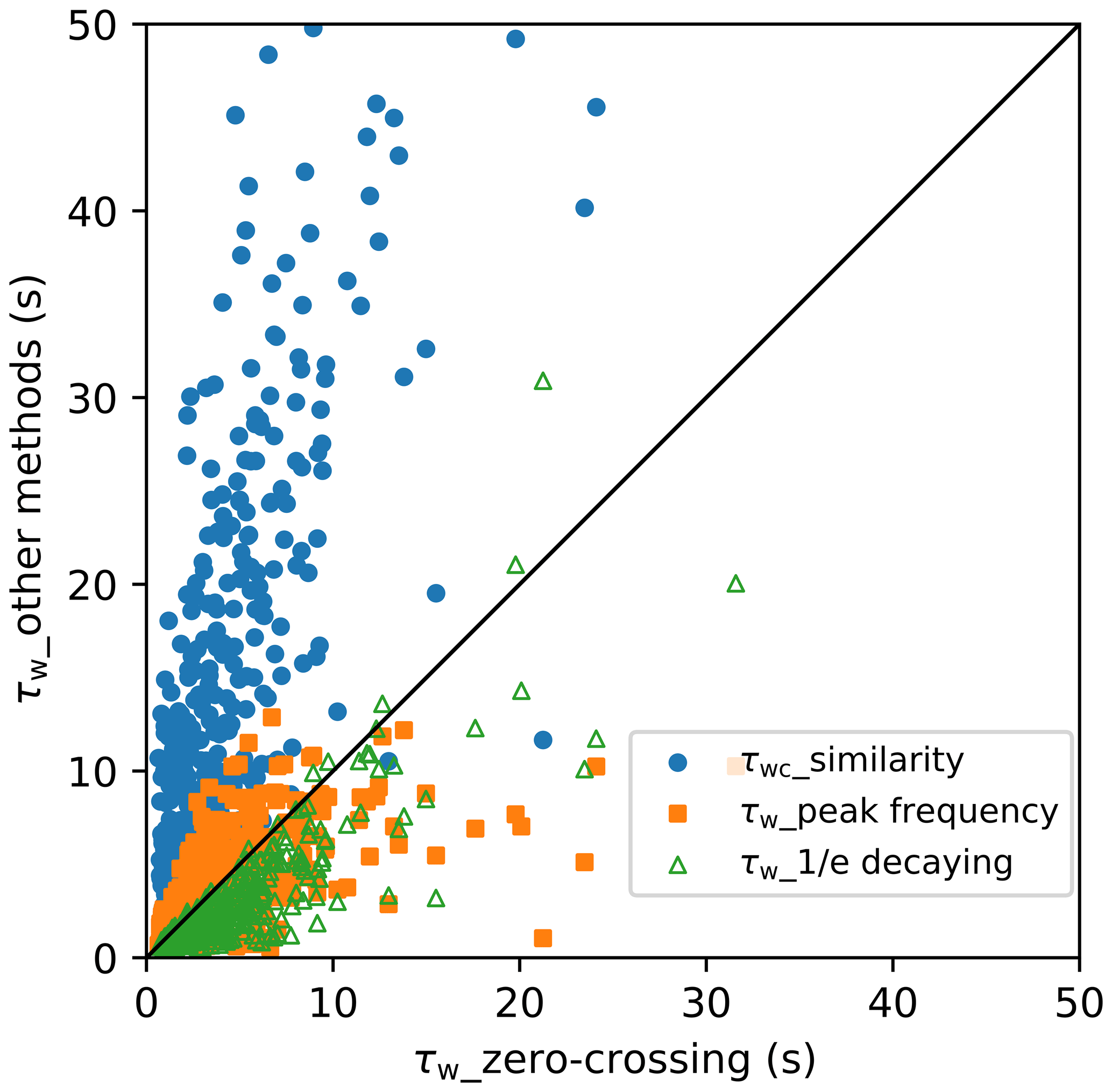
Figure B1 Comparison of integral timescales of w estimated by four different methods. Estimated integral timescales from the zero crossing method (integrating the auto-covariance function up to first zero crossing the function) agree well with the estimation of peak frequency method (Eq. B3). However, the similarity method (Eq. B2) overestimates the integral timescale, whereas the $\mathrm{1}/e$ decaying method (determining the time needed for the auto-covariance coefficient function value to decay to $\mathrm{1}/e$) tends to underestimate the integral timescale.

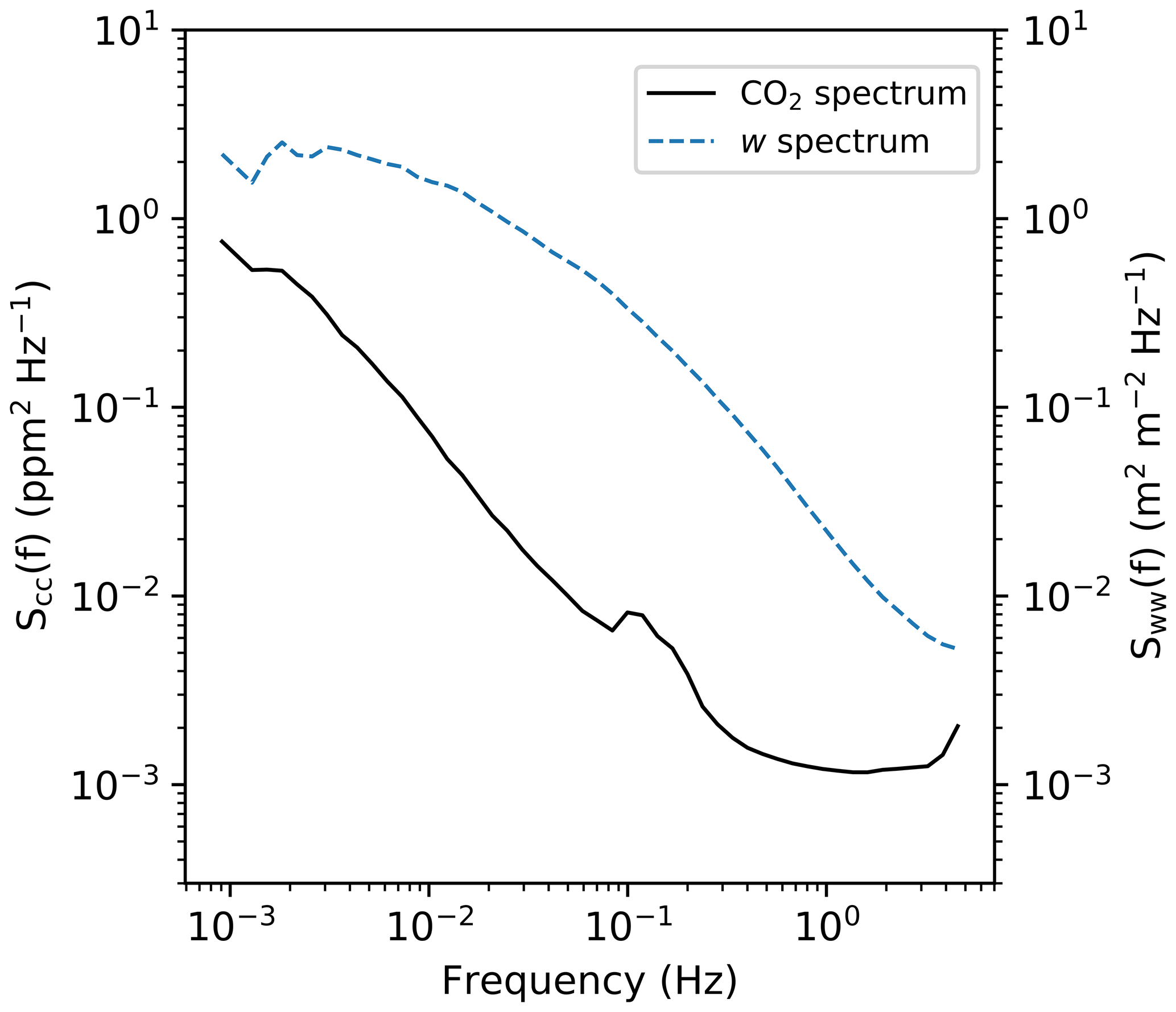
Figure B2 Mean variance spectra for CO₂ and w for one Arctic cruise JR18007. The near-constant CO₂ variance at high frequency (1–5 Hz) indicates the band-limited noise in the CO₂ signal. In contrast, the w spectrum does not show a similar band-limited noise at < 10 Hz.

The integral timescales of w estimated by these four methods for cruise JR18007 are shown in Fig. B1. The integral timescale estimated by the zero crossing method agrees well with the peak frequency estimates using Eq. (B3). The $\mathrm{1}/\mathrm{e}$ decaying method tends to underestimate the integral timescale, which is generally observed for turbulent signals (Rannik et al., 2009), whereas the similarity method (Eq. B2) considerably overestimates the integral timescale. Based on the recent analysis (as yet unpublished) of the entire NOAA PSL flux database, the Eq. (B2) formulation is now thought to be an overestimate (review comment for this paper from Blomquist, 2021). In this study we use the integral timescale of w from the zero crossing method to estimate the theoretical flux uncertainty (Eqs. 5 and 7). The theoretical systematic error estimates (Eq. 8) also require the integral timescale of CO₂. The integral timescale of CO₂ is difficult to evaluate from the above four methods due to instrument noise. Instead, we estimate it by directly integrating the auto-covariance function (Eq. B1) to a shift time of 200 s (we found no significant difference of the integral timescale when integrating the CO₂ auto-covariance function for shift times ranging from 150 to 250 s).

Appendix C: Comparison of the uncertainty estimates by different methods

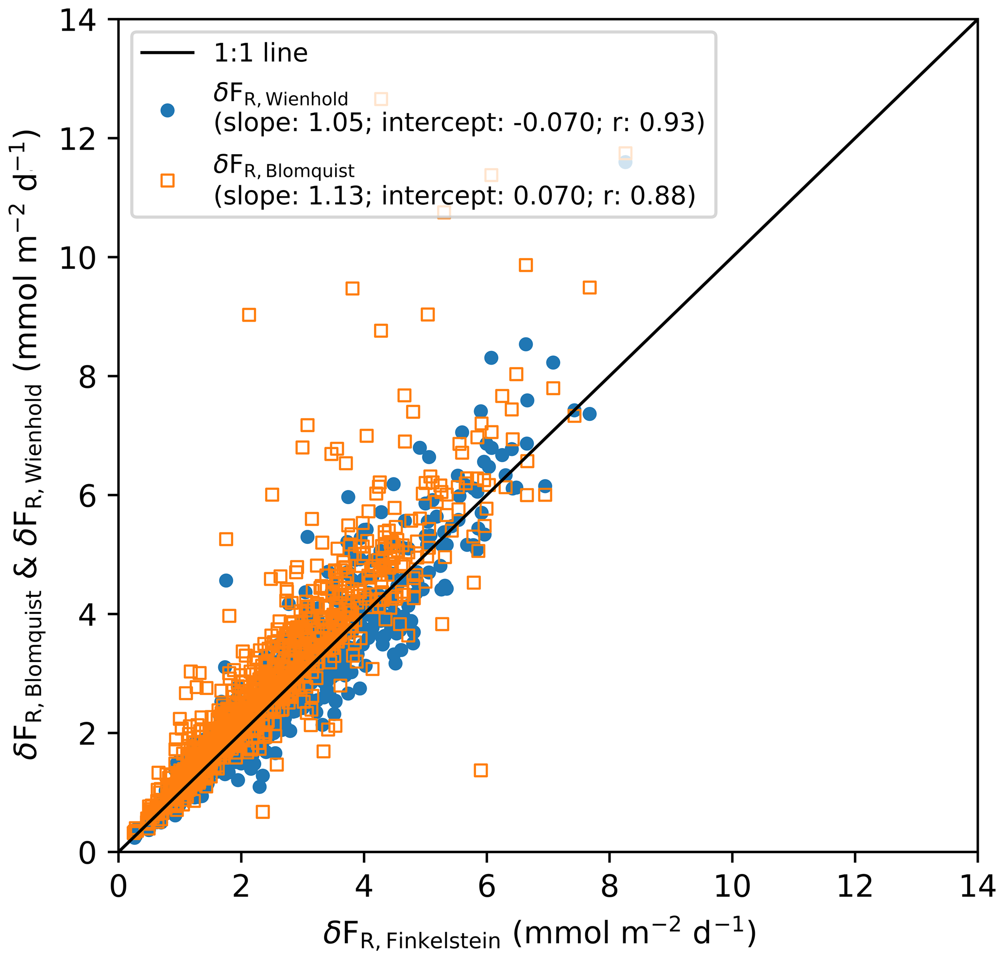
Figure C1 Comparison of total random uncertainties in hourly flux estimated by three different methods for the Arctic cruises. The empirical estimates F_R,Wienhold agree well with one of the theoretical estimates ΔF_{R,Finkelstein} (r=0.93). The other theoretical estimate ΔF_R,Blomquist is slightly higher than the random uncertainties ΔF_{R,Finkelstein} (slope = 1.13) if the constant in Eq. (8) is set equal to $\sqrt{\mathrm{2}}$.

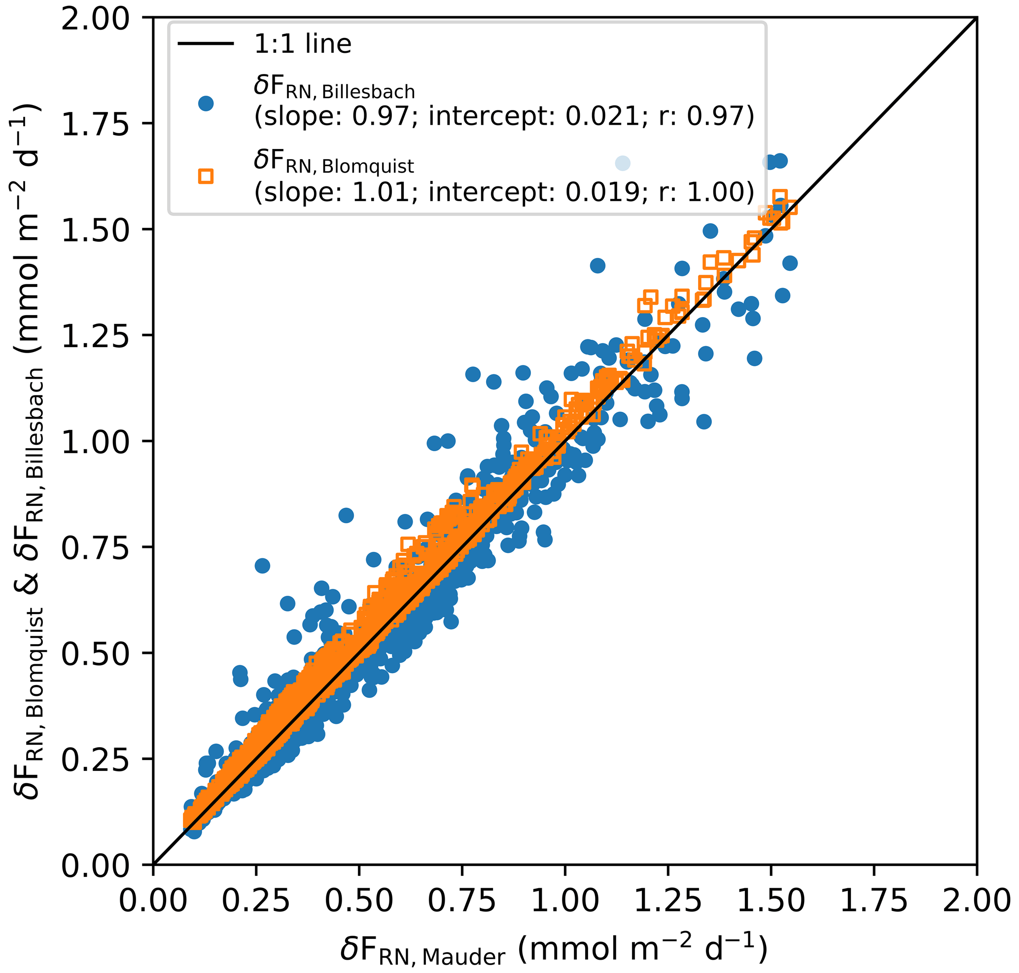
Figure C2 Comparison of random error in hourly flux due to instrument white noise, estimated by three different methods for the Arctic cruises. The three uncertainty estimations agree well. The correlation coefficient (r) between δF_RN,Mauder and δF_RN,Blomquist is 1 if the constant in Eq. (7) (a) is set to $\sqrt{\mathrm{2}}$.

Appendix D: Performance of two gas analysers

Figure D1 shows a comparison between the performance of the Picarro 2311-f and the LI-7200 gas analysers. We estimated that the noise of the LI-7200 is on average 3 times higher than that of the Picarro 2311-f (Table 3). Indeed, random error in the CO₂ flux due to the white noise is much higher for the LI-7200 than for the Picarro 2311-f, but the total flux uncertainty of the EC system with the LI-7200 on AMT29 is only slightly higher than that of the EC system with the Picarro 2311-f on AMT28 (Table 4). Again, this is because for both EC systems, sampling error dominates the total random uncertainty, while the contribution of instrument noise (< 30 %) to the total uncertainty is relatively small (Billesbach, 2011; Langford et al., 2015; Mauder et al., 2013; Rannik et al., 2016). Another often used CRDS gas analyser in EC measurements is the Los Gatos Research (LGR) Fast Greenhouse Gas Analyser (FGGA) (Prytherch et al., 2017). Yang et al. (2016) showed that LGR FGGA is ca. 10 times noisier than the Picarro G2311-f, and as a result, the total CO₂ flux uncertainty measured by the LGR is 4 times higher than that by the Picarro. From the perspective of measurement noise, Picarro and LI-7200 gas analysers are better suited for air–sea CO₂ flux measurements than the LGR FGGA.

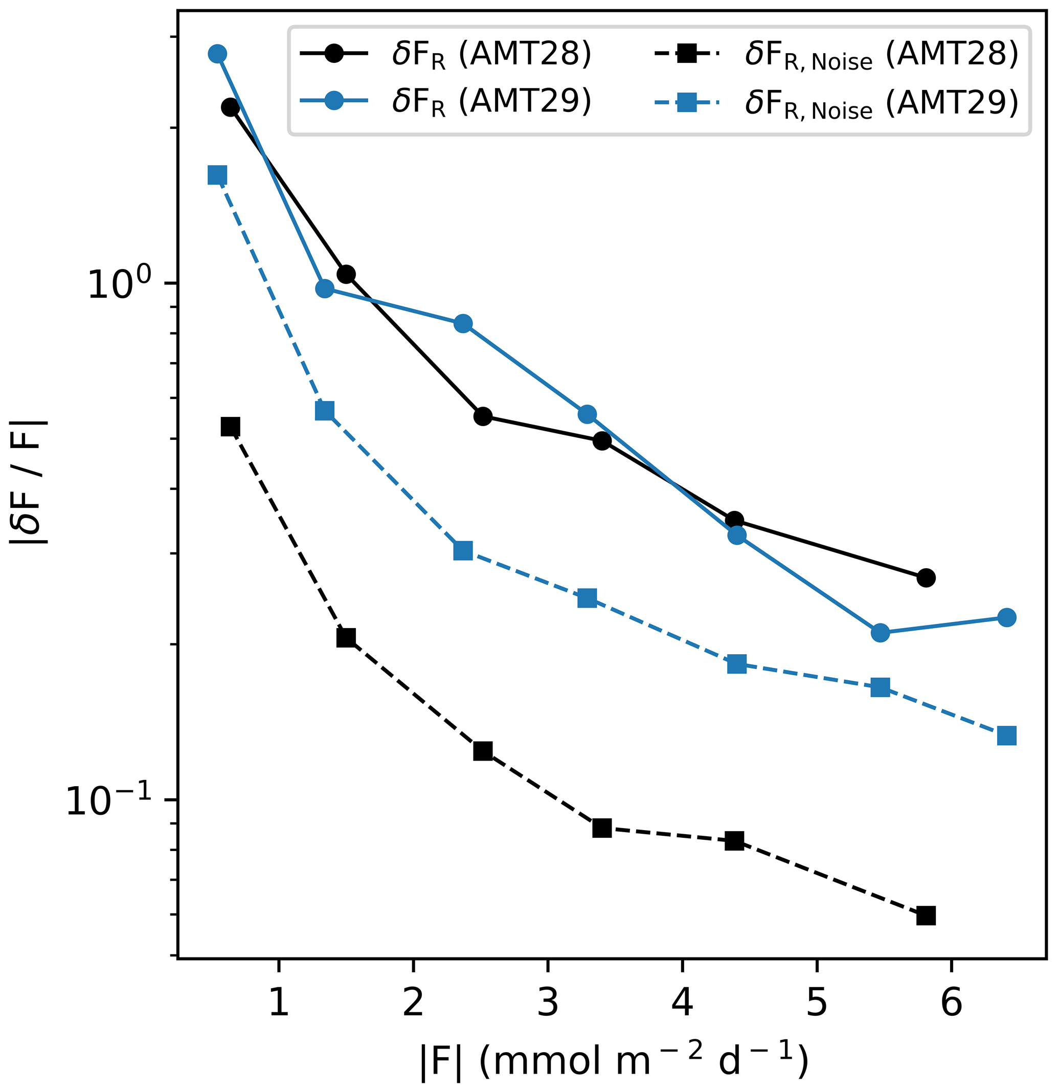
Figure D1 Comparison of the relative total random uncertainty and the relative random error component due to white noise for different gas analysers. A Picarro G2311-f gas analyser was used on AMT28 and a LI-7200 infrared gas analyser on AMT29.