Stratospheric gravity waves over the mountainous island of South Georgia: testing a high-resolution dynamical model with 3-D satellite observations and radiosondes

Atmospheric gravity waves (GWs) play an important role in atmospheric dynamics but accurately representing them in general circulation models (GCMs) is challenging. This is especially true for orographic GWs generated by wind flow over small mountainous islands in the Southern Ocean. Currently, these islands lie in the “grey zone” of global model resolution, where they are neither fully resolved nor fully parameterised. It is expected that as GCMs approach the spatial resolution of current high-resolution local-area models, small-island GW sources may be resolved without the need for parameterisations. But how realistic are the resolved GWs in these high-resolution simulations compared to observations? Here, we test a high-resolution (1.5 km horizontal grid, 118 vertical levels) local-area configuration of the Met Office Unified Model over the mountainous island of South Georgia (54^∘ S, 36^∘ W), running without GW parameterisations. The island's orography is well resolved in the model, and real-time boundary conditions are used for two time periods during July 2013 and June–July 2015. We compare simulated GWs in the model to coincident 3-D satellite observations from the Atmospheric Infrared Sounder (AIRS) on board Aqua. By carefully sampling the model using the AIRS resolution and measurement footprints (denoted as model sampled as AIRS hereafter), we present the first like-for-like comparison of simulated and observed 3-D GW amplitudes, wavelengths and directional GW momentum flux (GWMF) over the island using a 3-D S-transform method. We find that the timing, magnitude and direction of simulated GWMF over South Georgia are in good general agreement with observations, once the AIRS sampling and resolution are applied to the model. Area-averaged zonal GWMF during these 2 months is westward at around 5.3 and 5.6 mPa in AIRS and model sampled as AIRS datasets respectively, but values directly over the island can exceed 50 mPa. However, up to 35 % of the total GWMF in AIRS is actually found upwind of the island compared to only 17 % in the model sampled as AIRS, suggesting that non-orographic GWs observed by AIRS may be underestimated in our model configuration. Meridional GWMF results show a small northward bias (∼20 %) in the model sampled as AIRS that may correspond to a southward wind bias compared to coincident radiosonde measurements. Finally, we present one example of large-amplitude ($T^{\prime }\approx \mathrm{15}$–20 K at 45 km altitude) GWs at short horizontal wavelengths (λ_H≈30–40 km) directly over the island in AIRS measurements that show excellent agreement with the model sampled as AIRS. This suggests that orographic GWs in the full-resolution model with $T^{\prime }\approx \mathrm{45}$ K and λ_H≈30–40 km can occur in reality. Our study demonstrates that not only can high-resolution local-area models simulate realistic stratospheric GWs over small mountainous islands but the application of satellite sampling and resolution to these models can also be a highly effective method for their validation.

1 Introduction

Atmospheric gravity waves (GWs) are a key dynamical component of the Earth's atmosphere. Through the vertical transport of energy and momentum, these waves are an important coupling mechanism between atmospheric layers (e.g. Fritts and Alexander, 2003; Fritts et al., 2006). When they break or dissipate, GWs deposit a horizontal momentum forcing into the background flow, resulting in a drag or driving force that drives circulations away from states expected under radiative equilibrium.

But despite their importance, accurately representing GWs in global circulation models (GCMs) used for numerical weather and climate forecasting has proved challenging (Alexander et al., 2010; Plougonven et al., 2020). One reason for this is that a large fraction of GWs and their sources lie at physical scales that are below the spatial resolution of GCMs. The momentum forcing of these subgrid waves on the background flow must instead be simulated by parameterisations. (e.g. Warner and McIntyre, 1996; Kim et al., 2003; Alexander et al., 2010).

This is especially significant for small mountainous islands in the Southern Ocean. Observations reveal intense “hot spots” of stratospheric GW activity over these islands during austral winter (Alexander and Grimsdell, 2013; Hoffmann et al., 2013, 2016; Hindley et al., 2020), but due to their small size, islands like these lie in the grey zone of orographic GW parameterisations, where they are neither fully resolved nor fully parameterised (Vosper, 2015). Thus, orographic GW drag from small mountainous islands can often be inaccurately simulated in GCMs, which can in turn result in a significant underestimation of GW momentum (McLandress et al., 2012; Vosper et al., 2016; Garfinkel and Oman, 2018).

These islands also lie beneath a “belt” of intense wintertime GW activity at latitudes near 60^∘ S, which also includes the well-known hot spot of GW activity over the Southern Andes and Antarctic Peninsula. Gravity wave activity in this region and the surrounding 60^∘ S belt have been explored in numerous observational and modelling studies in the past 2 decades (Eckermann and Preusse, 1999; Jiang et al., 2002; de la Torre and Alexander, 2005; de la Torre et al., 2006; Hertzog et al., 2008; Alexander et al., 2009; Llamedo et al., 2009; Alexander et al., 2010; de la Torre et al., 2012; Plougonven et al., 2013; Hendricks et al., 2014; Alexander et al., 2015; Hindley et al., 2015; Wright et al., 2016b; Lilienthal et al., 2017; Hierro et al., 2018; Llamedo et al., 2019; Alexander et al., 2020).

Recent studies have suggested that “missing” GW momentum flux near 60^∘ S may be a significant contributing factor to the wintertime “cold-pole problem”, a significant and long-standing bias in nearly all major weather and climate models (Scaife et al., 2002; Butchart et al., 2011; McLandress et al., 2012; Alexander and Grimsdell, 2013; Garfinkel and Oman, 2018). The cold-pole problem refers to a simulated wintertime stratospheric polar vortex that is too cold by around 5 to 10 K, has winds that are too strong by around 10 m s⁻¹ and breaks up around 2 to 3 weeks too late into spring compared to observations (e.g. Butchart et al., 2011). This dynamical bias also causes difficulty in simulating chemical systems such as the stratospheric ozone cycle (e.g. Garcia et al., 2017), global chemical transport (e.g. McLandress et al., 2012) and surface climate change in the Antarctic (Thompson et al., 2011).

At larger horizontal scales of a few hundreds of kilometres, GWs can usually be directly resolved in current operational GCMs. To resolve GWs at fine horizontal and vertical scales, dedicated offline simulations are needed, which have provided encouraging results in recent years (e.g. Watanabe et al., 2008; Sato et al., 2012; Holt et al., 2017; Becker and Vadas, 2018). High horizontal resolution offline simulations can also be used to help improve GW parameterisations for subgrid-scale orography in operational GCMs (e.g. Vosper, 2015; Vosper et al., 2016, 2020).

Future advances in computing power will likely result in ever-finer horizontal and vertical grids in operational GCMs, which will enable the resolution of a large part of the GW spectrum. A question then arises, as posed by Preusse et al. (2014): in the future, will ever-higher spatial resolution in GCMs remove the need for GW parameterisations altogether? For orographic GWs from small mountainous islands, where spatial resolution is a key limiting factor in their representation, this seems to be a realistic possibility. But how realistic are simulated GWs in high spatial resolution simulations over these islands?

In this study, we address this question for one such island: South Georgia (54^∘ S, 36^∘ W) in the Southern Ocean. Despite being only around 170 km long, South Georgia is entirely mountainous with interior peaks exceeding 3000 m. During winter, the abrupt orientation of the topography relative to the strong prevailing wind provides favourable conditions for orographic GW generation and vertical propagation. Previous observational and modelling studies over South Georgia have revealed intense wintertime GW activity in the troposphere and stratosphere over the island (e.g. Alexander et al., 2009; Hoffmann et al., 2013; Vosper, 2015; Vosper et al., 2016; Hoffmann et al., 2016; Moffat-Griffin et al., 2017; Garfinkel and Oman, 2018; Jackson et al., 2018; Hindley et al., 2019, 2020).

To investigate simulated GWs over South Georgia, we use a dedicated high-resolution local-area configuration of the UK Met Office Unified Model (1.5 km grid, 118 vertical levels). The local-area model is nested in a real-date configuration for two time periods during July 2013 and June–July 2015, where lateral boundary conditions are provided by a global forecast, which ensures that simulated conditions are close to reality. No GW parameterisations are applied in the local-area model. After validating the model winds with coincident radiosonde observations, we compare simulated GWs over South Georgia to observed GWs in coincident 3-D satellite observations from AIRS/Aqua for the same time periods. By applying the vertical resolution, horizontal sampling and retrieval noise of the AIRS (Atmospheric Infrared Sounder) measurements to the model, we are able to make a direct like-for-like comparison of observed and simulated GW amplitudes, wavelengths and directional momentum fluxes over the island.

In Sect. 2 we describe the model, satellite and radiosonde datasets used in this study. In Sects. 3 and 4 we validate background winds in the model using the radiosonde observations and inspect the simulated GWs. Then in Sect. 5 we apply the AIRS resolution, sampling and retrieval noise to the model to make a fair comparison of GW measurements in AIRS and the model sampled as AIRS. A 3-D S-transform (3DST) analysis method for measuring GW properties is described in Sect. 6, after which we present a comparison of measured GW amplitudes, wavelengths and directional momentum fluxes over South Georgia in the model and satellite observations in Sect. 7. In Sect. 8 we investigate a case study of large-amplitude GWs at short horizontal wavelengths over the island. These results are discussed in Sect. 9, and we draw our conclusions in Sect. 10.

2 Data

Three atmospheric datasets over South Georgia are analysed in this study: (1) modelling simulations in a local-area domain centred on the island, (2) 3-D satellite observations from AIRS/Aqua and (3) radiosonde observations launched from the British Antarctic Survey (BAS) base at King Edward Point (KEP).

The spatial extent of these three datasets is shown in Fig. 1. South Georgia is located around 2000 km east of South America and the Antarctic Peninsula in the Southern Ocean. The 1200 km×900 km local-area modelling simulation over the island is shown by the light blue box in Fig. 1a, while the two dashed red and white boxes show two example overpasses of the AIRS instrument (one during an ascending node orbit and one during a descending node). Note that the exact location of each of the overpasses varies with each orbit, as discussed below. Figure 1b and c show 3-D views of these domains, through which the trajectories of radiosondes launched from the island during January and June–July 2015 are shown by dashed orange and green lines respectively. Note that the June–July radiosondes travelled much further downwind due to stronger stratospheric zonal winds during austral winter, and many of these travelled so far east that they exited the local-area model domain.

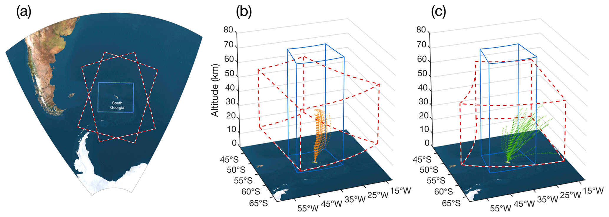
Figure 1 Maps showing the horizontal and vertical extent of the local-area model (blue lines) over the island of South Georgia and two examples of the typical extent of AIRS satellite measurements (dashed red and white lines) used in this study. Panel (a) shows a map of the local region around South Georgia, plotted on a regular distance grid. Panels (b and c) show the vertical extent of the model on a latitude–longitude grid. The vertical extent of usable temperature data from the 3-D AIRS retrieval scheme of Hoffmann and Alexander (2009) is shown in dashed red lines for both an ascending (b) and descending (c) overpass. Orange (green) lines show the trajectories of radiosondes launched from the island during a summer (winter) campaign in January (June–July) 2015.

2.1 Numerical modelling: local-area simulations over South Georgia

Here we use model output from specialised high-resolution runs of the UK Met Office Unified Model using the Even Newer Dynamics for General Atmospheric Modelling of the Environment (ENDGame) dynamical core (Davies et al., 2005; Wood et al., 2014). The model consists of a nested high-resolution local-area domain 1200 km×900 km around the island of South Georgia and is run in a real-date configuration with lateral boundary conditions supplied by a global forecast.

The nested local-area domain simulation consists of an 800×600-pixel latitude–longitude grid centred at 54.5^∘ S, 37.1^∘ W, with 118 vertical levels from the surface to altitudes near 80 km. The simulations are run in a rotated-pole coordinate frame in order to provide latitude–longitude spacing that is close to Cartesian. This grid gives a horizontal spacing of roughly 1.5 km×1.5 km, for which the island's orography is well resolved (Jackson et al., 2018). As described by Vosper (2015), a simultaneous run with a 750 m horizontal grid was also performed, but here we analyse the 1.5 km run due to computational constraints. Jackson et al. (2018) found no significant differences in the dominant stratospheric GW characteristics between these two runs, suggesting that the 1.5 km grid is sufficient to resolve the main features of the island's orography.

The vertical grid spacing of the local-area model increases from around 10 m near the surface to around 700 m at 25 km altitude and 1.9 km at 55 km altitude (Vosper, 2015, their Fig. 2). A damping layer is applied above 58.5 km altitude to suppress reflection effects near the model top. Sensitivity tests for vertical grids of 70, 118 and 173 vertical levels were performed by Vosper (2015). They found a high degree of similarity between resolved zonal GW momentum fluxes in the 118-level and 173-level simulations from the surface to altitudes near 40 km. Both of these configurations exhibited more realistic values than the 70-level simulation at high altitudes. Therefore, the 118-level configuration is selected to reduce the computational load and permit the use of a fine horizontal grid over the island. It should be mentioned that although this vertical grid spacing is sufficient to resolve wintertime orographic waves over South Georgia, the vertical grid spacing of around 1.5–2 km in the upper stratosphere is unlikely to accurately simulate body forces under wave breaking that are necessary for secondary GW generation (e.g. Becker and Vadas, 2018). The Unified Model uses a semi-Lagrangian dynamical core, so there is some implicit numerical diffusion as a result of the interpolation methods used to determine the departure points. In the local-area simulations used here, the “Smagorinsky-type” 3-D subgrid horizontal turbulence scheme is used (e.g. Pearson et al., 2014; Boutle et al., 2014, and citations therein).

Meteorological initial and lateral boundary conditions for the local-area domain are provided by a global N512 simulation with 70 vertical levels from the surface to altitudes near 80 km. At latitudes near South Georgia, this global model has a horizontal grid spacing of Δx≈46 km. This simulation is provided by Met Office operational analyses and re-initialised every 24 h, providing hourly forecasts that supply lateral boundary conditions for the local-area configuration over South Georgia. At the edges of the local-area domain, these hourly forecasts are linearly interpolated in time to the time step of the local-area model (30 s). As mentioned above, no orographic or non-orographic GW parameterisations were included in the local-area simulations. Output fields were archived hourly. More information on the configuration of these simulations is described in detail by Vosper (2015), Vosper et al. (2016) and Jackson et al. (2018).

The model run used here is for two time periods: 1 to 31 July 2013 and 11 June to 8 July 2015. These austral wintertime periods were chosen to coincide with the high probability of strong orographic GW forcing and deep vertical propagation due the strong prevailing winds at these latitudes during winter. A third model run for January 2015 was also conducted and analysed, but due to the weak stratospheric winds during austral summer, too few GWs (orographic or non-orographic) were visible in AIRS measurements for a meaningful comparison. Both model simulations during 2015 were designed to coincide with summer and winter radiosonde campaigns on South Georgia (Moffat-Griffin et al., 2017; Jackson et al., 2018) that are described below.

2.2 AIRS 3-D satellite observations

The Atmospheric Infrared Sounder (AIRS) (Aumann et al., 2003; Chahine et al., 2006) flies aboard NASA's Aqua satellite in a ∼100 min near-polar sun-synchronous orbit. AIRS is a nadir-sounding hyperspectral radiometer that measures radiances in 2378 infrared spectral channels in a continuous 90-element, ∼1800 km wide swath in the across-track direction at scan angles between $\pm \mathrm{49.5}{}^{\circ }$ from the nadir. The across-track horizontal spacing of these elements varies from around 13.5 km at nadir to 41 km at track edge.

Here we use 3-D AIRS temperature measurements derived using the retrieval scheme of Hoffmann and Alexander (2009). This retrieval uses multiple 4.3 and 15 µm CO₂ spectral channels to produce estimates of stratospheric temperature for each individual measurement footprint on a 3 km vertical grid. For each height level, retrieved temperatures have a vertical resolution related to the kernel functions of the selected AIRS channels used, which varies between 7–14 km for altitudes between 20 and 60 km (Hoffmann and Alexander, 2009; Hindley et al., 2019). The retrieval is optimised for GW analysis, where a balance is achieved between retrieval noise and vertical resolution. At high southern latitudes during winter, temperature measurement error is typically ≲1.5 K (Hoffmann and Alexander, 2009; Hindley et al., 2019). Validation of the 3-D AIRS temperature retrievals is described by Hoffmann and Alexander (2009) and Meyer and Hoffmann (2014).

There are typically two AIRS/Aqua overpasses per day over South Georgia, but due to the precession of the orbit, the locations of AIRS measurements during each overpass are not at the same geographic locations each day. For our study, we select only AIRS overpasses where the measurement swath covers at least three out of four corners of the local-area model domain, as shown in Fig. 1a. During the model runs in July 2013 and June–July 2015, we found that 39 and 48 AIRS overpasses respectively met this three-corner criterion, giving 87 coincident 3-D AIRS measurements in total for our comparison. These overpasses occurred within ±20 min of 03:00 and 17:00 UTC each day and measurements typically cover around 80 % to 90 % of the local-area model domain due to the high inclination of the AIRS/Aqua orbit.

2.3 Radiosondes

We also use wind measurements from radiosonde campaigns that took place on South Georgia during January (austral summer) 2015 and June–July (austral winter) 2015, the details of which are described by Moffat-Griffin et al. (2017). Balloons were launched twice daily from the British Antarctic Survey base at King Edward Point (54.3^∘ S, 37.5^∘ W), equipped with Vaisala RS92-SGP radiosondes, with additional launches timed to coincide with AIRS overpasses or when forecasts predicted strong winds suitable for GW generation. Meteorological and geolocation parameters are recorded at 2 s intervals during the flight.

The trajectories of the balloons are shown by the orange and green lines in Fig. 1b and c. Fifty-four balloons were successfully launched during the wintertime period of 13 June to 6 July 2015. Due to challenging local environmental conditions, 10 launches failed to reach the tropopause and only 20 reached altitudes of 25 km or above. During summer, nearly all of the 44 balloons launched reached their target altitudes near 35 km during January 2015. It can also be seen in Fig. 1c that during winter the balloons travelled much further downwind to the east than in summer due to the strong westerly wintertime winds. Several balloons were blown so far that they even travelled beyond the eastern boundary of the model domain, 600 km to the east, before reaching their final altitude. Wind measurements from these balloons are used to validate the direction and magnitude of the background wind in the local-area model to assess conditions for orographic GW generation and propagation. A comparison for both the summer and winter campaigns was performed, but due to reduced stratospheric GW activity in the model during summer, only a comparison for the wintertime measurements is shown below.

3 Model wind validation using co-located radiosonde measurements

Before we compare our simulated GW fields to satellite observations, we first use our co-located radiosonde observations to validate the model wind fields. Surface wind flow over orography is the key driver of mountain wave activity over the island (e.g Alexander and Grimsdell, 2013; Vosper, 2015; Moffat-Griffin et al., 2017; Jackson et al., 2018), and upper tropospheric and stratospheric winds determine the upward propagation of these orographically forced waves. Thus, model winds should first be tested to ensure they are a fair representation of reality before any GW investigations are undertaken.

The boundary conditions of the local-area model are initialised daily by Met Office operational analyses, but these winds are poorly constrained by conventional observations over the Southern Ocean, relying largely on temperatures nudged by assimilated satellite radiances. Wright and Hindley (2018) showed that a lack of observations can result in significant stratospheric biases in this region in global models. The radiosonde measurements described here are not assimilated into the operational analysis. Thus, to our knowledge, these radiosonde observations are the only coincident and independent wind measurements available to assess the tropospheric wind fields in the model over the island during our period of study.

Figure 2 shows hourly zonal and meridional wind against height for the two model runs during July 2013 and June–July 2015. These values are horizontally averaged over the whole model domain, so they are representative of the large-scale background flow. As would be expected for a wintertime study at these latitudes, wind speeds in the zonal direction are eastward and generally increase strongly with height, with values reaching 120 m s⁻¹ above 50 km altitude. In the meridional direction, frequent changes between northward and southward flow are observed, with speeds reaching values near ±40 m s⁻¹ above 40 km altitude. Gravity wave activity in the model for this time period is shown in panels e and f discussed later in Sect. 4.

Figure 2 Hourly zonal and meridional wind speeds against altitude in the local-area model over South Georgia during July 2013 (a, c) and June–July 2015 (b, d) averaged over a horizontal region 600 km×400 km centred on the island (region C in Fig. 4). Panels (e, f) show average zonal (blue) and meridional (orange) gravity wave momentum fluxes (GWMFs) $\stackrel{\mathrm{‾}}{\mathit{\rho }}\left(\stackrel{\mathrm{‾}}{u^{\prime }{w}^{\prime }},\stackrel{\mathrm{‾}}{v^{\prime }{w}^{\prime }}\right)$ over the same horizontal region but between 25 and 45 km altitude. Positive (negative) values indicate eastward (westward) zonal GWMF and northward (southward) meridional GWMF. Dotted lines in (e, f) show the percentage of the total model GWMF (right axis) downwind of the island (region B in Fig. 4), which is a strong indication of mountain wave activity.

To compare the model winds to radiosonde observations, each radiosonde trajectory is traced through the hourly model winds fields. Because of the large horizontal distances travelled by the radiosondes (up to 600 km) and the length of the flight times (up to around 2.5 h), it is necessary to evaluate the hourly model data along a path that varies in horizontal space, height and time. To do this, all hourly model outputs are loaded for the duration of each radiosonde flight, including 1 h before and 1 h after, and four-dimensional linear interpolants ($x,y,z,t$) of zonal u and meridional v wind fields are constructed. These interpolants are then evaluated for each point along the radiosonde's trajectory using the measured time, height and location of the balloon. This approach allows us to compensate for any time-varying effects in the model wind speeds during the radiosonde flights. The model winds along the radiosonde trajectories (denoted as model-as-sondes hereafter) are then compared to the radiosonde wind observations themselves. Figure 3a shows the results of our wind comparison. Radiosonde launch times (UTC) and maximum recorded altitudes during the winter campaign are shown by the black lines and circles in Fig. 3a. For illustration, the mean zonal wind speed over the modelling domain against altitude in also shown in panel a, which gives us an indication of the background wind conditions through which the balloons travelled.

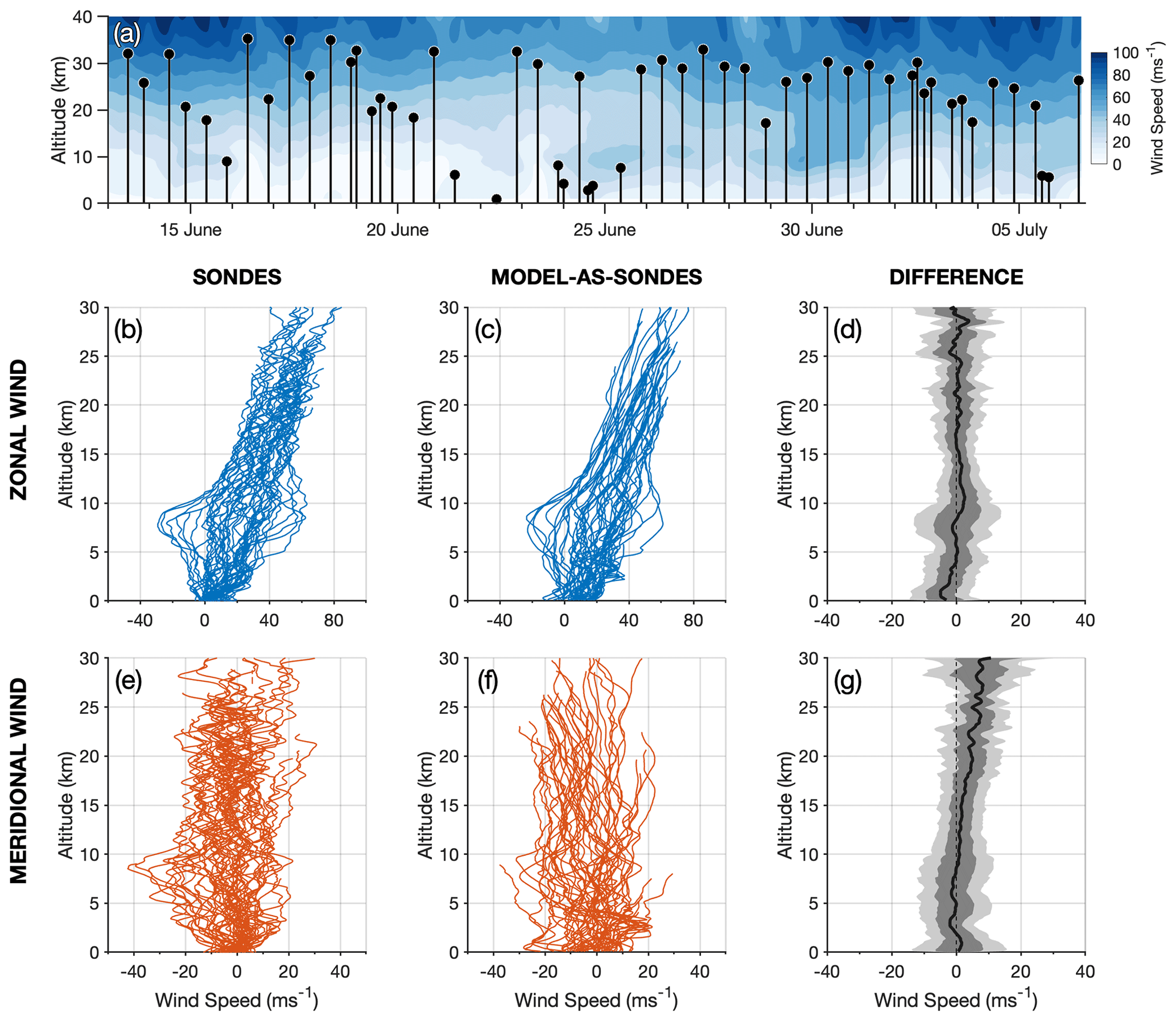
Figure 3 Comparison of wind speeds from the local-area model to coincident radiosonde observations launched from South Georgia during June–July 2015. Panel (a) shows launch times and maximum altitudes of the radiosonde observations (black lines), while coloured contours show the magnitude of the model wind speed for illustration. Panels (b, e, c, f) show profiles of zonal (blue) and meridional (orange) wind against height for the radiosonde measurements and the model wind, where the model wind has been evaluated along each radiosonde's trajectory. Panels (d, g) show the mean difference (thick black line) between the radiosonde and model wind speeds (the former minus the latter) for each height, while dark grey and light grey shading indicates 1 and 2 standard deviations respectively.

As can be seen in Fig. 3a, several of the radiosonde balloons did not reach their desired altitudes near 30 km, instead bursting soon after launch. This was usually due to the extreme weather conditions at low altitudes during the fieldwork campaign, as reported by the radiosonde launch team. In some cases, surface winds were so strong that radiosonde balloons did not ascend fast enough to exit the bay around the launch site, colliding instead with the slopes of nearby mountains.

Panels b–g in Fig. 3 show the measured radiosonde wind speed and the model wind speed evaluated along the radiosonde paths (model-as-sondes) in the zonal and meridional directions. The two datasets are in good general agreement, with measured and simulated zonal winds in Fig. 3b and c increasing from a few metres per second near the surface to around 60 m s⁻¹ near 30 km altitude. In the meridional direction, both datasets show wind speeds between around ±15 m s⁻¹ with little variation with altitude in Fig. 3e and f. The radiosonde measurements are found to exhibit more small-scale variability than the model fields, likely due to small-scale wave or turbulence features and measurement errors which are not present in the model. Some instances are also found where sonde measurements are present but no model-as-sonde data are available, which is due to the balloons horizontally exiting the model domain (see Fig. 1c).

To further compare the simulated and measured wind speeds, the difference between the sonde and the model-as-sonde winds (the former minus the latter) against altitude is shown in Fig. 3d and g for the zonal and meridional directions respectively. Shaded dark and light grey regions show 1 and 2 standard deviations of all differences respectively, while the thick black line shows the mean difference for the June–July 2015 run.

In the zonal direction, the time-averaged difference in wind speed is less than 5 m s⁻¹ for most altitudes above 10 km and close to zero in the low to mid-stratosphere between 15 and 25 km altitude. The largest differences between the sonde and model-as-sonde winds are seen for altitudes below 10 km in Fig. 3d. This is near the tropopause and could suggest that short-timescale variability of the tropospheric jet observed over the island is not so well represented in the model. This could influence the upward propagation of mountain waves. Near the surface, below altitudes of around 3 km, a slight bias towards stronger zonal winds in the model is observed. We suspect that this is due to slight underrepresentation of the “roughness” of the complex local topographic features around the launch site in the model. King Edward Point is located in a sheltered bay 2 km east of the main mountain ridge of the Thatcher Peninsula, which peaks at nearly 2 km high. At the 1.5 km model horizontal resolution used in this study, this mountain ridge will be at most one model grid cell away from the launch site. Thus, accurately simulating surface winds at this site will be quite challenging. Further, the model winds are not well constrained by surface observations in the area, so small surface biases are to be expected.

In the meridional direction, the time-averaged wind speed differences are generally less than 10 m s⁻¹ in Fig. 3g. However, a clear positive difference is observed above around 15 km altitude, which increases to near 10 m s⁻¹ at 30 km altitude. This indicates that the model slightly overestimates (underestimates) the southward (northward) winds in the mid-stratosphere. Because the mean difference is zero for the zonal component, this then not only tends in a small directional bias but also in a small positive bias in the net horizontal wind speed. Given that global models are very poorly constrained by conventional observations at high southern latitudes, this directional bias is actually quite reasonable. While we do not expect this to affect our results significantly, we acknowledge that a difference in the rotation of the simulated wind vector compared to reality could have an effect on wave propagation and thus the measured orientations of simulated mountain waves over the island.

It should be mentioned that some of the differences between the model and model-as-sonde winds could be due to timing or lag issues in the model, such as in the arrival of synoptic systems. Anecdotal reports from the radiosonde launch team on South Georgia suggested that the arrival of synoptic systems such as fronts and weather systems could differ from the Unified Model forecast by several hours. Although these are tropospheric phenomena, they may have a stratospheric response that is earlier or later than predicted. These would manifest as pseudo-random errors in our analysis, which could explain some of the spread in the wind speed differences. Aside from these differences, however, we conclude that overall the model wind speed and direction over the island is simulated reasonably well during the June–July 2015 campaign.

Caution should be taken when measuring gravity wave momentum fluxes from slanted vertical profiles through mountain wave fields (such as radiosonde measurements here). The usual assumptions required for the measurement of vertically integrated momentum fluxes of planar monochromatic waves do not hold true for mountain waves sampled with a slanted vertical profile (e.g. de la Torre and Alexander, 1995; de la Torre et al., 2018; Vosper and Ross, 2020). For this reason, we do not conduct a GW comparison between the model and the radiosonde measurements here and only use the radiosonde measurements to validate the model winds.

4 Gravity waves over South Georgia in the full-resolution model

After validating the simulated winds in our local-area model, we now consider simulated GW activity in the model. A key quantity in GW research is the vertical flux of horizontal pseudo-momentum, generally referred to as momentum flux. This property helps to quantify the vertical transfer of horizontal momentum by GWs. When a GW breaks, horizontal momentum will be deposited in the mean flow, resulting in a drag or driving effect on the background wind. Measuring and quantifying the momentum fluxes of mountain waves from small, isolated islands is an important area of current research (McLandress et al., 2012; Alexander and Grimsdell, 2013; Garfinkel and Oman, 2018; Jackson et al., 2018).

Figure 2e and f show zonal and meridional gravity wave momentum flux (GWMF) averaged between 25 and 45 km altitude and over a horizontal area 600 km×400 km centred on the island, denoted by region C in Fig. 4. Here, zonal GWMF F_x and meridional GWMF F_y are calculated as

$$\begin{array}{}\text{(1)}& \left(F_x,F_y\right)=\stackrel{\mathrm{‾}}{\mathit{\rho }}\left(\stackrel{\mathrm{‾}}{u^{\prime }{w}^{\prime }},\stackrel{\mathrm{‾}}{v^{\prime }{w}^{\prime }}\right),\end{array}$$

where ρ is the background atmospheric density; u^′, v^′, and w^′ are wind perturbations in the zonal, meridional, and vertical directions; and the overbar denotes an area average over GW scales (Fritts and Alexander, 2003; Ern et al., 2004). Wind perturbations u^′, v^′ and w^′ are separated from the background flow by subtracting a fourth-order polynomial fit in the zonal direction. This ensures reasonable consistency with the method used for the AIRS satellite observations described in Sect. 2.2, but the two methods are not identical and therefore should be considered separately.

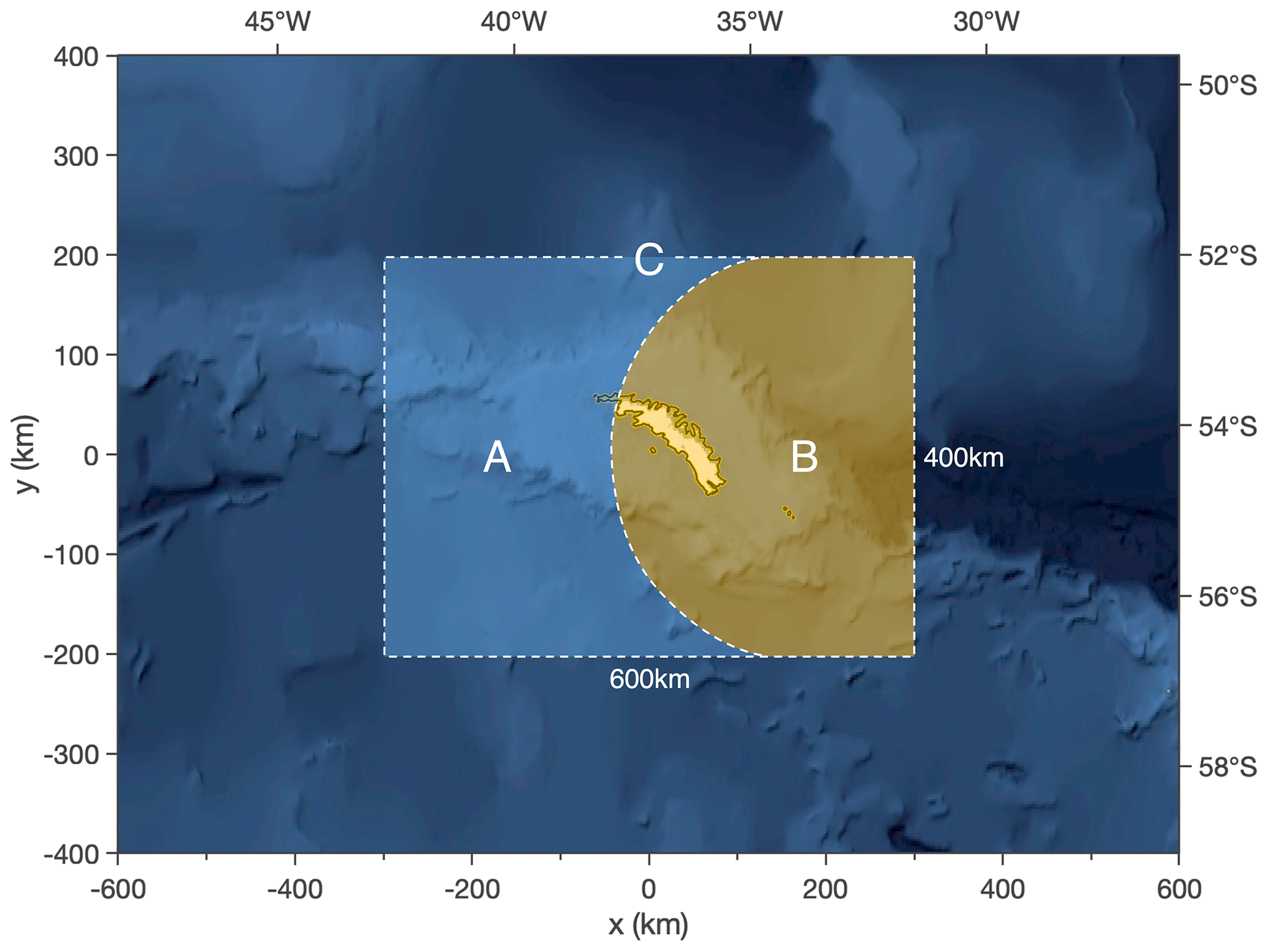
Figure 4 Illustration of the two regions to the east and west of South Georgia used to produce the values in Table 1. Region A is upwind of the island and region B is over and downwind of the island. The two regions have equal area.

Zonal and meridional GWMF time series in Figs. 2e and f indicate that stratospheric GW activity over the island in the full-resolution model is intermittent, with bursts of GWMF up to around 60 mPa occurring during 7–11 July 2013, 24–30 July 2013 and 4–6 July 2015. These bursts of GWMF generally coincide with periods of increased winds speeds from the surface through to the mid-stratosphere, as shown in Fig. 2a–d. This is indicative of strong mountain wave forcing by the surface winds and strong upper tropospheric and stratospheric winds that combine to provide good conditions for mountain wave propagation to greater heights. Indeed, during periods shown in Fig. 2a and b where the surface zonal winds are weak, stratospheric GWMF in Fig. 2e and f is low.

The average zonal direction of GWMF is generally westward, which is consistent with what we would expect for a mountain wave propagating against the background zonal wind in Fig. 2a. Interestingly, the area-averaged meridional GWMF is generally southward, regardless of the direction of the background meridional wind. For a typical mountain wave over an isolated island source, a characteristic bow-wave pattern is formed that has GWMF directed opposite to the wind but with additional northward and southward GWMF to the north and south. The distribution of GWMF around the island, shown later in this study, indicates that the southward component of this mountain wave field over the island (e.g. Alexander et al., 2009; Alexander and Grimsdell, 2013) is considerably larger than the northern component, likely due to the orientation of the island with respect to the background wind, which results in a southward area-average overall.

Dotted grey lines (right axes) in Fig. 2e and f show the percentage of the total absolute GWMF $(F_x^{\mathrm{2}}+F_y^{\mathrm{2}}{)}^{\frac{\mathrm{1}}{\mathrm{2}}}$ in region C contained within region B, located downwind of the island as shown in Fig. 4. Regions A and B have areas equal to half of region C, so a value of 50 % indicates a uniform distribution of GWMF between the upwind and downwind regions to the west and east of the island. A fraction larger than 50 % indicates more GWMF in the downwind region, which is a strong indication of mountain wave activity. It can be seen that during nearly all of the periods of increased GWMF in the model, this fraction is close to around 75 % to 100 %, which suggests that mountain waves are the dominant source of GW activity in the local-area model. This fraction rarely falls below 50 % and when it does it is during periods of low GWMF. This suggests that, relatively, non-orographic GW activity makes only a small contribution to the GWMF in the local-area model at full resolution.

5 Applying the AIRS observational filter to the model

The GWMF results in the previous section indicate significant GW activity in the full-resolution model. But these results cannot be directly compared to AIRS satellite measurements, because GW measurements in AIRS are subject to the AIRS observational filter. The observational filter (Preusse et al., 2002; Alexander and Barnet, 2007) is a key concept in GW observations. No single instrument or technique can measure the full GW spectrum. For example, the standard retrievals of nadir-sounding instrument such as AIRS will generally have relatively low vertical resolution (ΔZ≈15–20 km) for GWs in the stratosphere but relatively high horizontal resolution (ΔL≈50–100 km). In contrast, limb-sounding instruments and techniques such as HIRDLS (e.g. Gille et al., 2003) or GPS radio occultation (e.g. Kursinski et al., 1997) will have relatively high vertical resolution (ΔZ≈1 km) but relative low horizontal resolution (ΔL≈150–270 km). To make a fair comparison between GWs in our local-area model and coincident AIRS satellite observations, we must ensure that both datasets have the same observational filter.

For satellite observations, the observational filter is primarily dependent upon two things: sampling and resolution (Wright and Hindley, 2018). Below, we describe how we apply the sampling pattern and resolution of the AIRS observations to the local-area model to create a model-sampled-as-AIRS dataset that is comparable to the satellite observations.

5.1 Horizontal sampling

To create the model-sampled-as-AIRS dataset for our comparison to AIRS observations, we use hourly temperature output fields from the local-area model. As described above, model temperature fields are on a 1.5 km horizontal grid, with 118 vertical levels from the surface to near 70 km altitude.

The first step is to simulate the AIRS horizontal footprint and sampling pattern. The AIRS sampling pattern is well illustrated in Hoffmann et al. (2014, their Fig. 2). AIRS measurements are made on a 90-element wide horizontal across-track swath, where each measurement footprint is approximately 13.5 km×13.5 km wide (Hoffmann et al., 2014, their Table 1). The horizontal sampling distance between the centres of these footprints increases with increasing distance from the nadir from around 13.5 to 42 km near the track edge, so it is important to consider this for GWs with relatively short horizontal scales, such as those expected directly over South Georgia.

To simulate the AIRS measurement footprints in the model, each vertical level of each model temperature field is convolved with a horizontal Gaussian function with a full width at half maximum (FWHM) equal to 13.5 km×13.5 km. We then interpolate the smoothed model temperatures onto the horizontal sampling grid of the AIRS overpass that is closest in time to each hourly model output. The Gaussian smoothing step above ensures that this is a reasonable approximation to the horizontal sampling of an AIRS measurement footprint wherever the model is sampled. This gives us model temperatures at the horizontal sampling and resolution of the nearest coincident AIRS overpass to each hourly model output.

5.2 Vertical resolution

Next, we consider the vertical resolution of the AIRS measurements. To apply this vertical resolution to the model, we first need to interpolate the model onto a regular vertical grid. The chosen grid is from the surface to 75 km altitude in 1.5 km steps. This grid spacing is finer than the model vertical grid in the stratosphere but coarser in the troposphere. Because our comparison to AIRS measurements takes place in the stratosphere, this choice will not significantly affect our results.

The vertical resolution of the 3-D AIRS retrieval for different atmospheric conditions is shown in Fig. 2 of Hindley et al. (2019), where resolution values are derived using the approach of Hoffmann and Alexander (2009). The vertical resolution varies, on average, between 7 to 14 km between 20 and 60 km altitude. Using the values shown by Hindley et al. (2019), we apply the AIRS vertical resolution to the model temperature fields. This is a step-by-step process which involves the convolution of the model temperatures with vertical Gaussian functions with different FHWMs for each altitude. For example, the vertical resolution at 30 km altitude is approximately 7.5 km (Hindley et al., 2019, their Fig. 2b) so the full 3-D temperature volume is convolved with a vertical Gaussian function with FWHM equal to 7.5 km, and the horizontal level at 30 km altitude is then extracted and stored separately. This process is performed for each altitude level, allowing us to build up a smoothed temperature field, layer by layer, for each hourly model output. The result of this procedure is a 3-D volume of model temperatures sampled on the AIRS horizontal scan track and smoothed to the AIRS vertical resolution.

5.3 Retrieval noise

Finally, we consider the effect of AIRS retrieval noise. Noise in AIRS measurements can arise due to thermal noise in the AIRS instrument and/or deviations of the atmospheric state from local thermodynamic equilibrium, which is assumed in the retrieval (Hoffmann and Alexander, 2009). These factors vary for different spectral channels in the AIRS instrument, and as a result the estimated retrieval noise varies between 1.2 and 1.5 K between 25 and 45 km altitude, as shown in Fig. 2a of Hindley et al. (2019) and Fig. 5 of Hoffmann and Alexander (2009). However, because the retrieval noise is pseudo-random and incoherent in the horizontal, coherent wave features at large horizontal scales with amplitudes slightly below these noise values can be detected under reasonable conditions (Hindley et al., 2019). In the general case however, we cannot routinely separate retrieval noise from GW perturbations in AIRS measurements, and so to rule out the possibility of retrieval noise affecting our comparison, we add specified AIRS retrieval noise to our the model sampled as AIRS.

To apply the AIRS retrieval noise to the model, we select an AIRS overpass at 17:00 UTC on 20 June 2015 (granule numbers 174 and 175) containing no discernible wave features at any altitude level. Once the background temperature is removed using the method below, the residual perturbations exhibit an approximate standard deviation of around 0.5 K at 39 km altitude. For each altitude level, the residual noise perturbations from this overpass are randomised and then added to the model temperature fields for each hourly model output to simulate AIRS retrieval noise. The use of synthetic random Gaussian noise was considered for this purpose, but since AIRS noise characteristics vary with altitude, we found that using genuine AIRS noise provided more realistic results.

6 Measuring 3-D gravity wave properties

To investigate the properties of the GWs over South Georgia in our AIRS and model-sampled-as-AIRS datasets, we first extract GW temperature perturbations from the background; then we measure GW properties using the 3-D S-transform spectral analysis technique.

6.1 Extracting gravity waves temperature perturbations

As a result of the steps in the previous section, the temperature data for each hourly model-sampled-as-AIRS output lie on the same grid as the nearest AIRS overpass. This means that we can use the same background removal method to extract GW temperature perturbations from both datasets. This is important because it ensures that our analysis method does not introduce differences in the spectral range of GWs visible to each dataset that would invalidate our comparison.

To extract GW temperature perturbations at each altitude level, a horizontal fourth-order polynomial fit is performed in the across-track direction for each cross-track row (e.g. Wu, 2004; Alexander and Barnet, 2007; Hoffmann et al., 2014; Wright et al., 2017; Hindley et al., 2019). Slowly varying background signals due to large-scale temperature gradients or planetary wave activity are contained in this fit. This is then subtracted from each cross-track row to reveal residual GW perturbations.

As a result of the steps above, our AIRS and model-sampled-as-AIRS temperature perturbations are sensitive to GWs with vertical wavelengths between 8≲λ_z≲40 km, as defined by the AIRS vertical resolution. In the horizontal, the sensitivity cutoff for short horizontal wavelengths is determined by the AIRS footprint spacing (2 × 13.5 km = 27 km at nadir and 2 × 40 km = 80 km at the scan edges). For longer horizontal wavelengths, sensitivity falls below 90 % for λ_H≳700 km and below 10 % at λ_H≳1400 km as a result of the fourth-order polynomial background fit (Hoffmann et al., 2014). Sensitivity functions for the 3-D AIRS retrieval to stratospheric GWs can be found in Hindley et al. (2019), Hoffmann et al. (2014) and Ern et al. (2017).

Because the AIRS temperature retrieval has reduced vertical resolution and accuracy outside the height range 20 to 60 km altitude (Hoffmann and Alexander, 2009), we set AIRS and model-sampled-as-AIRS GW perturbations outside this range to zero and apply a half-bell tapering window to the upper and lower boundaries. This minimises any impact of edge effects in our subsequent spectral analysis.

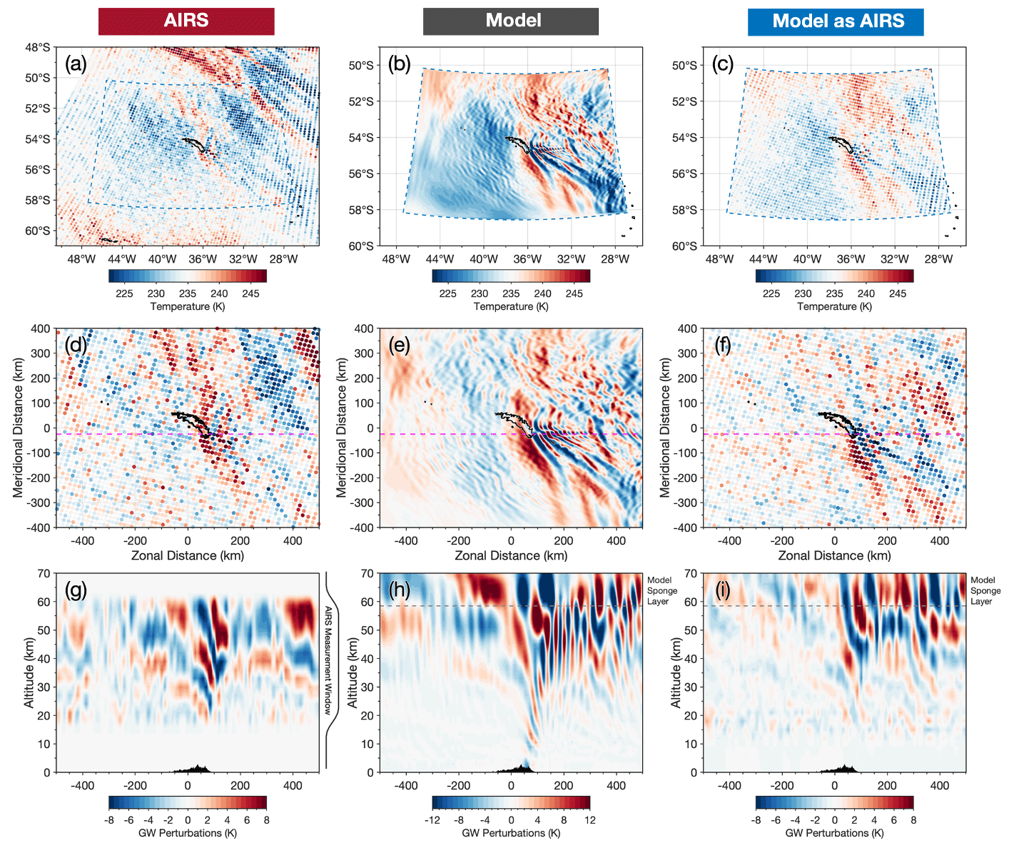
Figure 5 Observed and modelled temperatures (a–c) and temperature perturbations (d–f) at 45 km altitude over South Georgia at 03:00 UTC on 5 July 2015 in AIRS measurements, the full-resolution local-area model and the model sampled as AIRS. Coloured circles in (a, c) and (d, f) indicate the size and locations of the AIRS measurement footprints. The bottom row shows vertical cuts through the temperature perturbations along the dashed pink line in (d–f). See Sect. 5 for details on the model-sampled-as-AIRS data.

Figure 5 shows temperature measurements near 45 km altitude from AIRS, the full-resolution model and the model sampled as AIRS during an AIRS overpass at 03:00 UTC on 5 July 2015. Coloured circles in a, c, d, and f show the locations and horizontal sampling of the AIRS measurements footprints for this overpass. The dashed blue line denotes the horizontal boundary of the model domain.

Characteristic bow-wave patterns are visible over South Georgia in all three datasets in Figs. 5a–c. These are typical of orographic “mountain waves” from a small isolated island source. These features are apparent as GW perturbations in Fig. 5d–f. Significant fine-horizontal-scale wave structure is also visible in the full-resolution model, where temperature perturbations exceed ±12 K directly over the island. The horizontal scales and amplitudes of GW perturbations in the AIRS and model-sampled-as-AIRS datasets, however, show good qualitative similarity, with GW amplitudes around 6–8 K over the island in both datasets. The addition of the AIRS retrieval noise in the model sampled as AIRS is also apparent in Fig. 5c and f.

Figure 5g–i show a vertical cut through the AIRS, model and the model sampled as AIRS temperature perturbations along the dashed pink line shown in panels d–f. Both AIRS and model-sampled-as-AIRS measurements are limited to between 20 to 60 km altitude, where the retrieval is most reliable (Hoffmann and Alexander, 2009), but for this example we show the full height range of data in the model sampled as AIRS for completeness. Westward-sloping GW phase fronts with increasing altitude are found over the island in each of the datasets. These are characteristic of upwardly propagating mountain waves subject to eastward prevailing winds (e.g. Vosper, 2015). Again, the full-resolution model in Fig. 5h exhibits large-amplitude wave structure at short horizontal scales (λ_H around 30–40 km) over the island and up to around 300 km to the east. However, once the AIRS vertical resolution and horizontal sampling is applied in the model sampled as AIRS (Fig. 5i), these short-horizontal-scale structures are diminished, and the remaining wave structures with larger horizontal scales (λ_H≈50–150 km) are qualitatively similar to the wave features found in AIRS in Fig. 5g. While it is not expected that the phase structure of the mountain wave field in the model and observations should match exactly, the agreement is reasonable. This example indicates that the horizontal and vertical scales of GWs in the model sampled as AIRS show good qualitative agreement with GWs observed in AIRS.

To the north-east of the island in Fig. 5a, a large-horizontal-scale GW structure is observed in the AIRS measurements. Close inspection of this example suggests that the phase fronts shown in the AIRS vertical cut in Fig. 5h between 300 and 500 km east of the island are part of this same wave structure. We find that wave structures of this kind are commonly observed in AIRS measurements in the region during winter (e.g. Hindley et al., 2019, their Fig. 1), but their origin is unclear (Hendricks et al., 2014). Due to their physical scale and orientation, waves like this example are unlikely to have originated from South Georgia.

No clear evidence of this wave is found in the model or the model sampled as AIRS, but this is not unexpected. The global forecast that supplies the lateral boundary conditions for our local-area model has a coarse vertical grid, with only 70 vertical levels from the surface to near 80 km, so GWs such as this one are unlikely to be accurately simulated. Furthermore, even if they are accurately simulated, it is not clear how realistically these GWs would be transferred through the model boundary conditions into the local-area model. As a result, we expect our model and model-sampled-as-AIRS temperature fields to underrepresent GWs of this kind. This is discussed further in Sect. 9.

6.2 Measuring gravity wave properties with a 3-D S-transform

In Sect. 4 we used directional wind perturbations u^′, v^′ and w^′ to estimate GW momentum flux in the full-resolution model via Eq. (1). However, AIRS can only measure GW temperature perturbations, so we must use these to make our comparison between AIRS and the model sampled as AIRS.

We can use spatially localised measurements of GW temperature amplitudes T^′, horizontal wavenumbers k and l, and vertical wavenumber m to estimate directional GWMF in AIRS and model-sampled-as-AIRS measurements via the relation

$$\begin{array}{}\text{(2)}& \left({\text{MF}}_x,{\text{MF}}_y\right)={\displaystyle \frac{\mathit{\rho }}{\mathrm{2}}}{\left({\displaystyle \frac{g}{N}}\right)}^{\mathrm{2}}{\left({\displaystyle \frac{\left|T^{\prime }\right|}{\stackrel{\mathrm{‾}}{T}}}\right)}^{\mathrm{2}}\left({\displaystyle \frac{k}{m}},{\displaystyle \frac{l}{m}}\right),\end{array}$$

where MF_x and MF_y are the zonal and meridional components of GWMF, ρ is atmospheric density, g is the acceleration due to gravity, N is the buoyancy frequency, and $\stackrel{\mathrm{‾}}{T}$ is the background atmospheric temperature (Ern et al., 2004). Zonal, meridional and vertical wavenumbers k, l and m are related to spatial wavelengths as $k=\mathrm{2}\mathit{\pi }/{\mathit{\lambda }}_x$, $l=\mathrm{2}\mathit{\pi }/{\mathit{\lambda }}_y$ and $m=\mathrm{2}\mathit{\pi }/{\mathit{\lambda }}_z$ respectively. This relation is valid for mid-frequency GWs, where the intrinsic frequency ${\widehat{\mathit{\omega }}}^{\mathrm{2}}\gg f^{\mathrm{2}}$, where f is the inertial frequency (Fritts and Alexander, 2003). Ern et al. (2017) showed that this relation is valid for GWs within the spectral range visible to AIRS.

To obtain spatially localised measurements of GW amplitudes and wavelengths, we use a 3-D adaptation of the S-transform (also known as the Stockwell transform). Developed by Stockwell et al. (1996), the S-transform is a widely used spectral analysis technique that can localise and measure the amplitudes of individual frequencies (or wavenumbers) in a time series or distance profile. The S-transform has been applied for GW analysis in a variety of geophysical datasets (e.g. Fritts et al., 1998; Stockwell and Lowe, 2001; Alexander and Barnet, 2007; Alexander et al., 2008; Stockwell et al., 2011; McDonald, 2012; Wright and Gille, 2013; Alexander, 2015; Sato et al., 2016; Hindley et al., 2016; Wright et al., 2017; Hindley et al., 2019; Hu et al., 2019a, b; Hindley et al., 2020) and has also been applied in a variety of other fields, such as the planetary (Wright, 2012), engineering (Kuyuk, 2015) and biomedical sciences (e.g. Goodyear et al., 2004; Brown et al., 2010; Yan et al., 2015).

Here we use the N-dimensional S-transform (NDST) software package as described by Hindley et al. (2019). This version builds on the work of previous multidimensional S-transform analysis by Hindley et al. (2016) and Wright et al. (2017) but applies a superior wave amplitude measurement technique and features a much faster computational methodology which reduces computation time by around a factor of 10 compared to previous 3DST versions for AIRS analysis. A step-by-step guide describing how the 3DST method is applied to 3-D AIRS measurements is described in Hindley et al. (2019, their Sect. 3).¹ Validation of the 3DST analysis method using synthetic wave fields can be found in Hindley et al. (2016) and Hindley et al. (2019).

To make meaningful 3DST measurements of wavelengths, a regular orthogonal grid is required. The AIRS and model-sampled-as-AIRS datasets have irregular across-track spacing (Fig. 5), so we interpolate the GW temperature perturbations for each AIRS overpass and each hourly model-sampled-as-AIRS output onto a 10 km×10 km horizontal grid centred on South Georgia. This is finer than the horizontal sampling of the AIRS grid, so aliasing effects are unlikely to be significant. If any aliasing effects do occur, their effects will be equal for the AIRS and the model sampled as AIRS, so this will not affect our comparison. In the vertical, we interpolate onto a 1.5 km vertical grid which is finer than the stratospheric vertical grids (and vertical resolutions) of both the AIRS retrieval and the model. This regridding is therefore unlikely to affect our results.

We apply the 3DST to regularly gridded GW temperature perturbations for 87 three-dimensional AIRS measurements and 1320 hourly model-sampled-as-AIRS outputs during July 2013 and June–July 2015. Following the approach of Hindley et al. (2019), we set the 3DST scaling parameter $c_x=c_y=c_z=\mathrm{0.25}$ and analyse for the 1000 largest-amplitude wave signals with wavelengths greater than 27, 27 and 6 km in the x, y and z directions respectively. These are Nyquist sampling limits of twice the smallest separation of original AIRS sampling pattern (2 km×13.5 km) in the horizontal, and twice the spacing of original vertical grid of the AIRS retrieval (2×3 km). Because both datasets are analysed on the same regular grid, the exact same frequencies are to be analysed for both. These steps provide spatially localised measurements of GW temperature amplitudes, wavelengths and directions for the AIRS and model-sampled-as-AIRS datasets.

6.3 Case study comparison of 3-D gravity wave properties in AIRS and the model sampled as AIRS

We inspect 3DST measurements of GW properties in AIRS and the model sampled as AIRS for an AIRS overpass at 17:00 UTC on 5 July 2015 in Figs. 6 and 7. This overpass occurs 14 h after the example shown in Fig. 5 and is one of the most intense examples of mountain wave activity observed during the time periods of the model runs. The purpose of this case study comparison is not only to compare the model sampled as AIRS to the AIRS observations but also to confirm that we can measure the 3-D properties of the dominant wave structure with the 3DST.

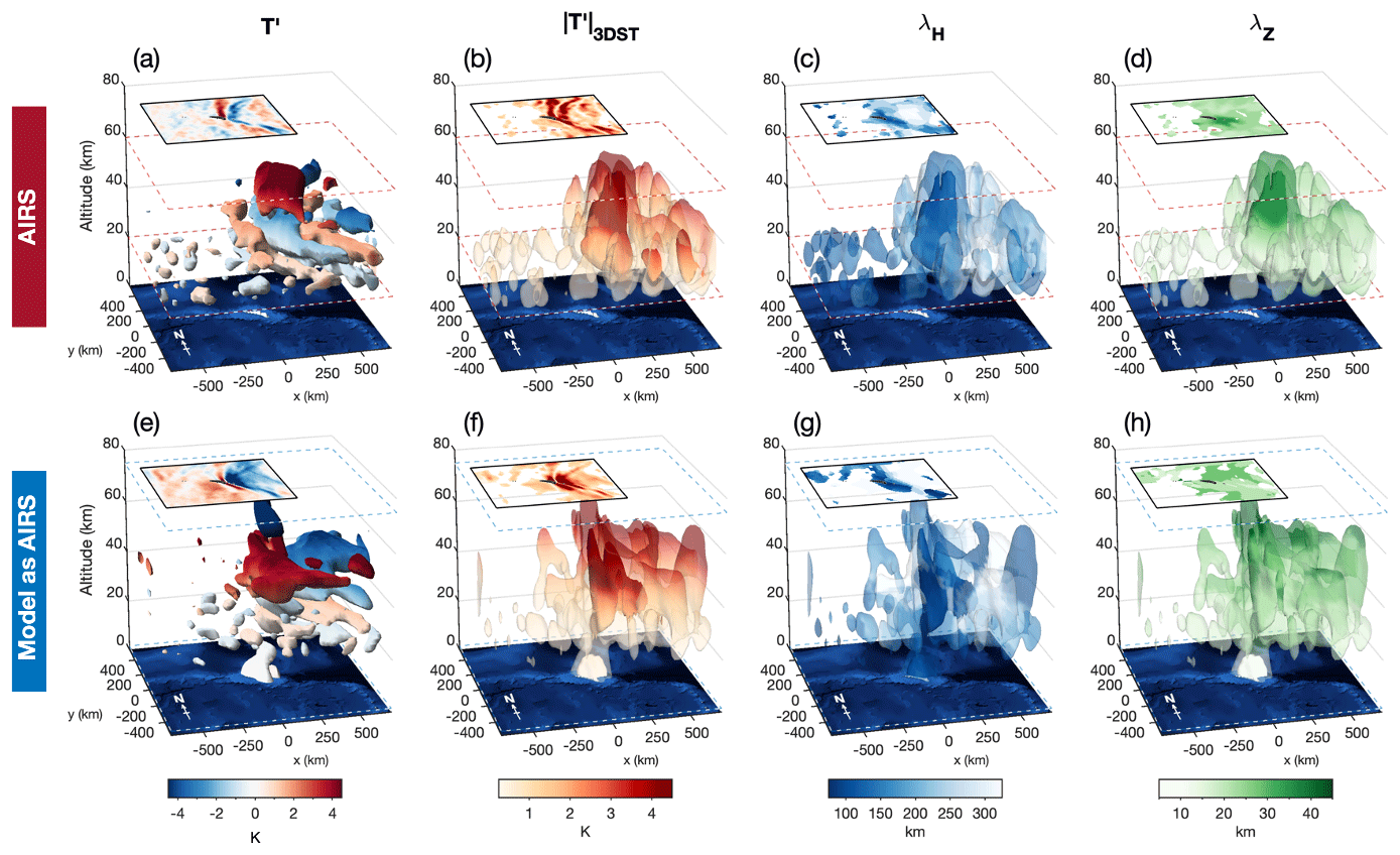
Figure 6 The 3-D S-transform (3DST) analysis of temperature perturbations from AIRS satellite observations (a–d) and the model sampled as AIRS (e–h) over South Georgia for 17:00 UTC on 5 July 2015. Coloured isosurfaces in (a, e) show the AIRS and model-sampled-as-AIRS temperature perturbations T^′, while (b, f), (c, g), and (d, h) show 3DST-measured absolute wave amplitude $|T^{\prime }{|}_{\text{3DST}}$, horizontal wavelength λ_H, and vertical wavelength λ_z respectively. Dashed blue and dashed red lines denote the upper and lower boundaries of the model domain and the AIRS measurements respectively. Horizontal cuts through the data at 40 km altitude are shown in the top left corners of each panel, which share a colour scale with the isosurfaces.

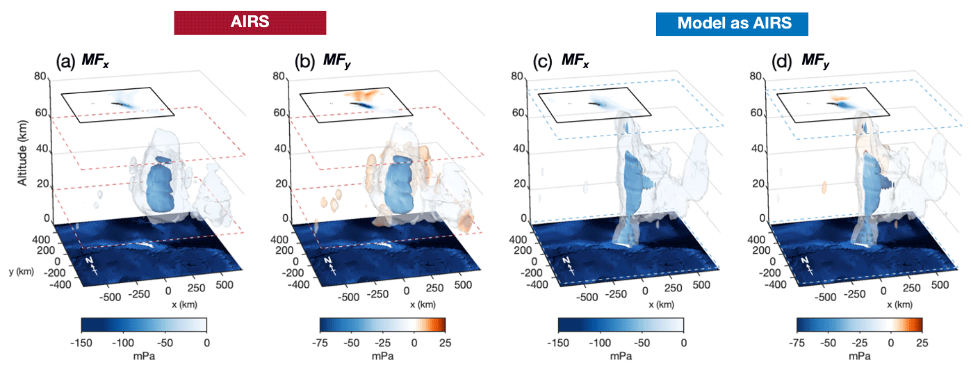
Figure 7 Same as Fig. 6 but for the zonal and meridional components of gravity wave momentum flux MF_x and MF_y for the AIRS and model-sampled-as-AIRS data at 17:00 UTC on 5 June 2015. In this example, westward propagation has been assumed based on sequential model results, indicating quasi-stationary mountain wave phase fronts with time subject to eastward wind conditions. This allows us to constrain the directional ambiguity in the zonal and meridional measurements.

6.3.1 3DST measurements of GW amplitude and wavelength

Figure 6 shows the 3DST analysis results for AIRS measurements (a–d) and the model sampled as AIRS (e–g) at 17:00 UTC on 5 July 2015. Input temperature perturbations are shown in panels a and e, and measured wave amplitudes are shown in panels b and f. Horizontal wavelengths (λ_H) are shown in panels c and g, and vertical wavelengths (λ_z) are shown in panels d and h. In each panel, a horizontal cross section through the data at an altitude of 40 km is overlaid in the top left corner, which shares a colour scale with the isosurfaces. The extents of the AIRS and model data are shown by dashed red and dashed blue lines respectively. In this figure, a 3×3-element horizontal boxcar filter has been applied to make the isosurfaces smoother for visual clarity.

In both the AIRS measurements and the model sampled as AIRS, temperature perturbations exhibit a bow-wave pattern, which is characteristic of a mountain wave field over a small isolated island such as South Georgia (e.g. Vosper, 2015). The largest wave amplitudes are localised over the island in both datasets, where values exceed 5 K at 40 km altitude directly over and immediately downwind of the island. The leeward “wings” of the mountain wave field that extend to the north and south are more prominent in AIRS measurements than in the model sampled as AIRS, but measured wave amplitudes closer to the island are comparable. As in Fig. 5, real and specified retrieval noise is apparent in the AIRS and model-sampled-as-AIRS temperature perturbations respectively, as we intended.

Figure 6c and g show measured horizontal wavelengths, ${\mathit{\lambda }}_{\mathrm{h}}=({\mathit{\lambda }}_x^{-\mathrm{2}}+{\mathit{\lambda }}_y^{-\mathrm{2}}{)}^{-\frac{\mathrm{1}}{\mathrm{2}}}$, for the AIRS and the model sampled as AIRS respectively. In both datasets, short horizontal wavelengths, λ_h<50–100 km, are located in a vertical column directly over the island. The bow-wave patterns to the north and south exhibit longer measured horizontal wavelengths of around 200 km in AIRS but shorter wavelengths at around 150 km in the model sampled as AIRS.

Away from the island, long horizontal wavelengths are measured. This is due to a design choice in our 3DST analysis. For regions with no clear wave activity, only retrieval noise is present. The wavelength limits and scaling parameter settings in our 3DST analysis are designed so that the dominant measured horizontal wavelength in these regions is long (λ_H≳600–1200 km), analogous to a horizontal “flat field”, following the approach of Hindley et al. (2019). In practice, we find that this choice is advantageous, because measurements of incoherent small-scale retrieval noise could otherwise be confused with measurements of short horizontal wavelength GWs (Alexander et al., 2009; Hindley et al., 2016, 2019). Other studies, such as Ern et al. (2017), choose to measure these regions as having short horizontal wavelengths using the S3D method of Lehmann et al. (2012).

Measured vertical wavelengths for AIRS and the model sampled as AIRS are shown in Fig. 6d and h. Vertical wavelengths are found to increase with altitude in both datasets. This is consistent with the expected refraction of mountain waves that are subject to increasing background wind speed with altitude, as indicated by the model winds in Fig. 2a and b. It is also consistent with the reduced vertical resolution of the AIRS retrieval with increasing height above around 40 km altitude (Hoffmann and Alexander, 2009, their Fig. 5). In the AIRS measurements, longer vertical wavelengths, λ_z≳35–40 km, are found directly over and immediately to the east of the island near 40 km altitude. In the model sampled as AIRS, vertical wavelengths are slightly shorter, with λ_z≳25–35 km near 40 km altitude. This could help to explain why the measured AIRS GW temperature amplitudes in Fig. 6b exhibit slightly larger values than in the model sampled as AIRS. If the real GW structure exhibited a slightly longer vertical wavelength compared to the simulated GW, this would increase the sensitivity of AIRS to this wave, resulting in larger measured temperature amplitudes. This could arise due to slightly stronger wind speeds than simulated in the model. Unfortunately, the radiosondes launched from South Georgia on the afternoon of 5 July 2015 did not reach their intended altitudes (Fig. 3a) due to extreme weather conditions reported at the launch site, so we cannot investigate this further for this example.

6.3.2 Zonal and meridional momentum fluxes

Figure 7 shows zonal and meridional momentum fluxes MF_x and MF_y calculated using Eq. (2) for measured GW properties in AIRS and the model sampled as AIRS at 17:00 UTC on 5 July 2015. As in Fig. 6, horizontal cross sections through the data at an altitude of 40 km are overlaid in the top left corner of each panel.

To show directional GWMF, we must also break a directional ambiguity in our 3-D measurements. Because each AIRS overpass only provides observations for a single moment in time, we cannot distinguish between GWs that propagate “upwards and forwards” or “downwards and backwards” (Wright et al., 2016a). For the example in Fig. 6, we inspected the time-varying wave structure in the model-sampled-as-AIRS temperature fields to determine that the simulated wave is a quasi-stationary westward-propagating mountain wave subject to eastward wind conditions. This means we can confidently break the directional ambiguity for this example and assume westward propagation, since the agreement in the mountain wave structure between the AIRS and the model sampled as AIRS is good. But this is not possible for all AIRS and model-sampled-as-AIRS measurements in our study, because not all measured waves are expected to be clear mountain waves. In the general case, therefore, we assume upward propagation (m<0) for observed waves in all subsequent results. This follows the approach of several previous studies involving AIRS measurements (Ern et al., 2017; Wright et al., 2017; Hindley et al., 2019, 2020). Ern et al. (2017) and Hindley et al. (2020) found that a realistic horizontal directionality of global stratospheric GWMF can be obtained by making this upward assumption.

The largest GWMF values in Fig. 7 are observed in a vertical column directly over the island in both the AIRS and model-sampled-as-AIRS wave fields. These regions coincide with the largest wave amplitudes, shortest horizontal wavelengths and longest vertical wavelengths in Fig. 6. Zonal momentum fluxes are directed westward, with values between 50–150 mPa over the island. Meridional GWMF is predominantly directed southward over the island, with values between 50–75 mPa in both datasets, indicating a south-westward direction of the net GWMF. A northward component of MF_y is also found to the north of the island. This is an encouraging result that suggests our 3DST analysis is correctly localising the diverging meridional components of the characteristic bow-wave pattern to the north and south of the island.

7 Gravity wave properties in AIRS and the model sampled as AIRS over South Georgia

The examples shown in Sect. 6 demonstrate that the AIRS sampling and resolution can be applied to the model to make a comparable model-sampled-as-AIRS dataset. We then showed that wave amplitudes, wavelengths and directional momentum fluxes can be measured using a 3DST method in a case study example. Here, we apply this method to all available AIRS observations and hourly model-sampled-as-AIRS outputs during the model runs in July 2013 and June–July 2015.

7.1 Time series of wave amplitude and directional GWMF

Figure 8 shows measured wave amplitudes and zonal and meridional momentum fluxes against time for AIRS and model-sampled-as-AIRS measurements. Values are averaged over a horizontal region 600 km×400 km centred on the island (region C in Fig. 4) between 25 and 45 km altitude. The shaded grey areas in Fig. 8 show the extent of the 10th and 90th percentiles of measured wave amplitude and GWMF over this region for AIRS (light grey) and the model sampled as AIRS (dark grey) respectively.

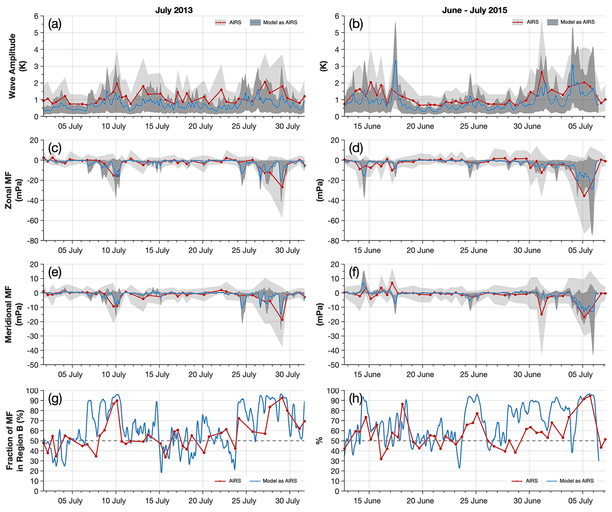
Figure 8 Time series of median GW amplitudes and net zonal and meridional momentum fluxes derived from AIRS measurements (red) and the model sampled as AIRS (blue) for July 2013 and June–July 2015. Values are averaged between altitudes of 25 and 45 km over a horizontal region 600 km×400 km centred on the island (region C in Fig. 4). Red circles show the overpass times of the AIRS measurements. Light and dark shaded grey areas show the 5th and 95th percentiles of measured wave amplitudes and momentum fluxes over the same region for AIRS and the model sampled as AIRS respectively. As in Fig. 2, panels (g and h) show the percentage of the total GWMF measured downwind of South Georgia (region B in Fig. 4). Percentage values larger 50 % are a good indication of mountain wave activity.

The time series in Fig. 8 indicate that GW activity over South Georgia is highly intermittent during our period of study. Several time periods of increased gravity activity are observed in both the AIRS and the model sampled as AIRS, such as during 7–11 July and 24–31 July 2013 and during 14–16 June, 24–26 June, and 29 June–6 July 2015. Figure 8a and b indicate that during these events, area-averaged GW amplitudes increase to around 1–2 K. The shaded percentile regions, however, reveal that some locations in the region can exhibit much larger amplitudes during these periods, where the 90th percentile of measured amplitudes can exceed 5 K. This is consistent with the large wave amplitudes measured over the island in the examples in Figs. 5 and 6 for the overpasses on 5 July 2015.

The time series of net zonal and meridional momentum fluxes in Fig. 8c–f also reveal high intermittency. During periods of increased GW activity, area-averaged GWMF values are found to increase to around 20–40 mPa in the zonal direction and 10–20 mPa in the meridional. As with the wave amplitudes, the 10th and 90th percentile shading regions indicate that peak GWMF values in the region reached much higher values, exceeding 70 mPa in the zonal direction and 40 mPa in the meridional during the largest wave events in July 2015.

The directionality of net zonal and meridional GWMF in Fig. 8c–f is generally negative for both AIRS and the model sampled as AIRS, indicating a predominantly south-westward net direction. This is consistent with the results for the case study in Fig. 7, but we should recall here that for this time series we assumed upward propagation for all measured waves. The fact that the horizontal directionality agrees well with the case study example, where westward propagation was assumed, gives us additional confidence in the directionality of our measured GWMF values. Further, we can see from Fig. 8f that during the mountain wave event on 5 July 2015, the shaded percentile regions reveal increased northward and southward meridional momentum fluxes, although the southward component is dominant. This is consistent with the northward and southward components of a characteristic mountain wave field from an island source (e.g. Vosper, 2015).

Panels g and h in Fig. 8 show the percentage of the total GWMF in region C that was contained in region B, as illustrated in Fig. 4. Since region C is made up of the two regions A and B, both of which have equal area, this percentage provides us with a useful metric for determining how much of the total GWMF was distributed upwind or downwind of the island. This metric is useful, because it is consistent for both the AIRS and model-sampled-as-AIRS GWMF measurements.

During periods of increased wave activity, a larger percentage of the total GWMF is usually measured downwind of the island in region B in both datasets. This is a strong indication of mountain wave activity, since we would normally expect that non-orographic wave activity would be distributed more evenly over regions A and B, although we acknowledge this may not always be the case. During periods around 29 July 2013 and 5 July 2015, however, where large GWMF values are measured, over 90 % of the total GWMF was contained downwind of the island in region B in both AIRS and the model sampled as AIRS. Inspection of the temperature perturbations during these events revealed characteristic bow-wave mountain wave patterns downwind of South Georgia. During periods of relatively low wave activity, such as during 15–23 July 2013 or 19–24 June 2015, then this percentage is close of 50 %, indicating a relatively uniform distribution of GWMF over regions A and B.

The agreement between the AIRS measurements and the model sampled as AIRS in Fig. 8 is generally reasonable. The timing and magnitude of increased GWMF found during GW events is similar between the two datasets. However, although GWMF results indicate similar magnitudes, GW temperature amplitudes in the model sampled as AIRS are consistently around 20 %–30 % smaller than found in AIRS. One reason for this could be due to the use of the area average. If AIRS measurements exhibit more GW activity at large distances from the island, which could be indicative of non-orographic GW activity, this would lead to a larger area average. But the shaded percentile regions in Fig. 8a and b also indicate that the 90th percentile of measured amplitudes in AIRS is consistently larger than in the model sampled as AIRS by a similar amount. This suggests that large-amplitude events in AIRS also exhibit larger amplitudes than their counterparts in the model sampled as AIRS. These results are discussed further in Sect. 9.

7.2 Horizontal distributions of wave amplitude, λ_H and directional GWMF

The horizontal distribution of GW properties around South Georgia is shown in Fig. 9. For this analysis, measured GW amplitudes, horizontal wavelengths λ_H, and zonal and meridional momentum fluxes for AIRS and the model sampled as AIRS are averaged over 25 to 45 km altitude for all measurements during July 2013 and June–July 2015. For λ_H, only values for GWs with amplitudes $T^{\prime }>\mathrm{1.5}$ K are included in the average (Hindley et al., 2019).

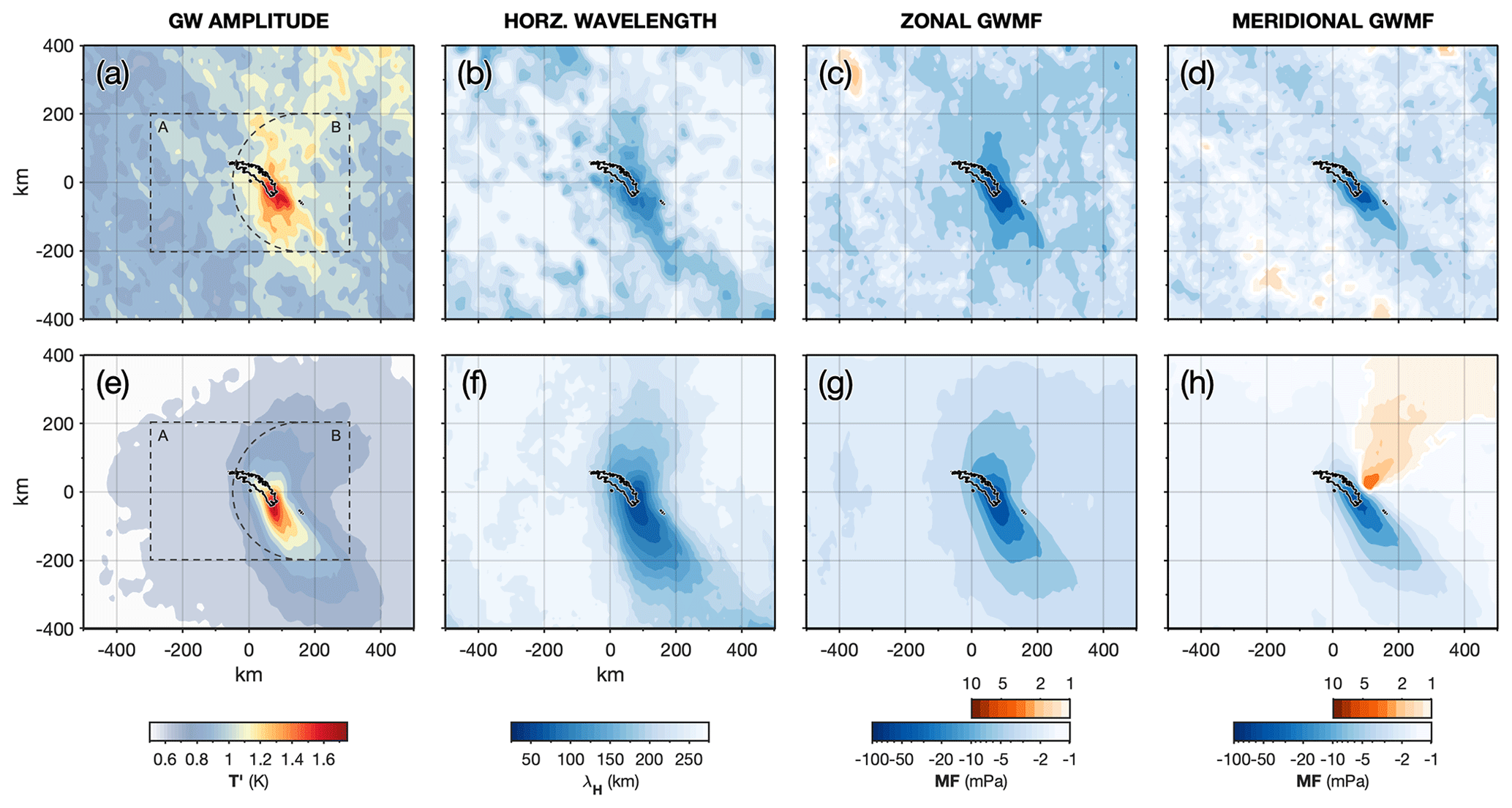
Figure 9 Average GW temperature amplitudes T^′, horizontal wavelengths λ_H, and zonal and meridional momentum flux (GWMF) MF_x and MF_y over South Georgia from AIRS measurements (a–d) and the model sampled as AIRS (e–h) during both modelling campaigns in July 2013 and June–July 2015. Data are averaged over a vertical region between 25 and 45 km altitude. For horizontal wavelengths, only λ_H measurements for GWs with amplitudes $T^{\prime }>\mathrm{1.5}$ K are included in the average. Black dashed lines in (a) and (e) show the extent of the regions described in Fig. 4.

Average GW amplitudes in Fig. 9a and e exceed 1.5 K directly over the island in both AIRS and the model sampled as AIRS for this 2-month period. Both datasets exhibit increased GW amplitudes directly over the island and in a region extending around 150 km to the south, but AIRS exhibits regions of increased GW amplitudes further to the north and south in a somewhat disorderly pattern. To the east and west of the island, GW amplitudes near 0.9 K are measured in AIRS compared to just 0.7 K in the model sampled as AIRS.

Because we added specified AIRS retrieval noise to the model sampled as AIRS, it is unlikely that this difference is due to noise in AIRS measurements. Instead, it may be due to non-orographic GWs (NGWs) in the real atmosphere that are not well represented in this local-area model configuration. Recent satellite and modelling studies have suggested significant NGW activity can be found in this region during winter (e.g. Sato et al., 2012; Choi and Chun, 2013; Hendricks et al., 2014; Plougonven and Zhang, 2014; Hindley et al., 2015; Polichtchouk and Scott, 2020; de la Cámara et al., 2016). Even if such NGWs are poorly resolved by AIRS, their partial detection creates general variability and anisotropy in the AIRS temperature perturbations, which are then measured as GW amplitudes in our 3DST analysis. Direct inspection of the AIRS measurements suggests that this effect is quite different from the effects of pixel-scale retrieval noise and does not appear in the model sampled as AIRS. This is discussed further in Sect. 9.

The shortest average horizontal wavelengths in Fig. 9b and f are found directly over the island, with values around 60 and 80 km in the model sampled as AIRS and AIRS respectively. But caution should be taken when considering time-averaged wavelengths. The characteristic horizontal wavelength of a generalised mountain wave field directly over the island is related to the size of the orographic obstacle in the direction of the prevailing wind. This is around 30–40 km for South Georgia under westerly wind conditions. The fact that both datasets exhibit longer horizontal wavelengths over the island suggests that other (probably non-orographic) waves with longer λ_H are included in the average. Because AIRS exhibits around 30 % longer average horizontal wavelengths over the island than in the model sampled as AIRS, this could indicate that NGWs with $T^{\prime }>\mathrm{1.5}$ K are more often found in the AIRS observations here.

Zonal GWMF in Fig. 9c and g is almost entirely westward, which is consistent with expected propagation of GWs into the background wind. Over the island, westward GWMF exceeds 50 mPa in both datasets. Meridional GWMF in Fig. 9h exhibits a north–south divergence in the model sampled as AIRS that is centred on the island. This is characteristic of a bow-wave mountain wave field. We recall here that we did not specify this horizontal directionality and only upward propagation was assumed. This further suggests that our assumption of upward propagation for GWs visible to AIRS during winter in this region is generally valid. We acknowledge, however, that any downwardly propagating waves (m>0) will exhibit the opposite horizontal directionality ($k\to -k$ and $l\to -l$) in our analysis due to being mislabelled as upwardly propagating. Our results here, however, do not suggest that this has a significant effect on the directionality of our measured GWMF over long timescales and, even if such an effect is present it would be equal for both AIRS and the model sampled as AIRS, so it would not affect the validity of our comparison.

Both the AIRS and the model sampled as AIRS exhibit large southward GWMF of more than 50 mPa to the south of the island in Fig. 9d and h, but only the model sampled as AIRS exhibits a clear northward component in this time average, albeit at comparatively weak values of up to 4 mPa. One reason for this could be due to the small meridional wind bias in the model wind shown in Sect. 3. We found that the model exhibited a southward wind bias of up to 10 m s⁻¹ between 15 to 30 km altitude compared to coincident radiosonde observations. Although our radiosonde measurements do not extend further than 30 km, it is possible that this observed wind bias could persist to altitudes between 25 and 45 km, where our GWMF measurements in Fig. 9 are shown. This southward wind bias could lead to a stronger northward section of the simulated mountain wave field than is observed in AIRS, due to the preferential propagation of mountain waves into the background wind.

Table 1 Measured GW amplitudes and directional momentum fluxes in upwind (A) and downwind (B) regions of South Georgia in the full-resolution model, AIRS observations and the model sampled as AIRS. Values are averaged between 25 and 45 km altitude over regions A and B (see Fig. 4) for all GW measurements during July 2013 and June–July 2015. The two rightmost columns show the fractions of total absolute GWMF in region C that were measured in regions A and B. Note that GWMF in the full-resolution model is calculated using Eq. (1), but AIRS and the model sampled as AIRS GWMF is calculated via Eq. (2).

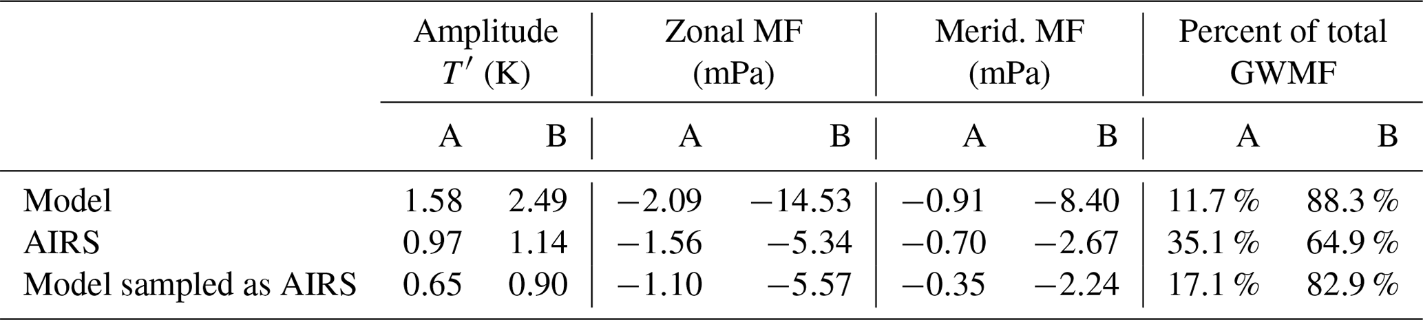
The results of Fig. 9a–f are summarised in Table 1 over the two regions A and B. Here, average wave amplitudes and net GWMF are shown for AIRS, the model sampled as AIRS and full-resolution model for all GW measurements during July 2013 and June–July 2015. Note that amplitudes and GWMF in the full-resolution model are not directly comparable to values in the AIRS or the model sampled as AIRS, due to the different observational filter and processing methods, but they are included for context.

All three datasets exhibit larger wave amplitudes and net GWMF in region B (downwind) than in region A (upwind), but average wave amplitudes in region B in the model sampled as AIRS are around 20 % smaller than found in AIRS. Despite this, average GWMF values in region B are similar, where the magnitude of the net flux $({\text{MF}}_x^{\mathrm{2}}+{\text{MF}}_y^{\mathrm{2}}{)}^{\frac{\mathrm{1}}{\mathrm{2}}}$ in both datasets is around 6 mPa. This suggests that because average λ_H over the island is longer in AIRS than in the model sampled as AIRS, the larger average wave amplitudes in AIRS do not lead to larger GWMF values via Eq. (2).

The two rightmost columns of Table 1 show the fractions of the total absolute GWMF measured upwind and downwind of the island. Around 35 % of the total GWMF in AIRS is found upwind of the island in region A compared to only 17 % in the model sampled as AIRS. Further, the magnitude of the net GWMF in the upwind region is around 45 % larger in AIRS than in the model sampled as AIRS. These results indicate that the model sampled as AIRS may underestimate NGW activity upwind of South Georgia compared to observations.

There is also a small difference in the direction ${\tan }^{-\mathrm{1}}\left({\text{MF}}_x/{\text{MF}}_y\right)$ of the net GWMF in region B between the AIRS and the model sampled as AIRS, which exhibit directions of 243 and 248^∘ clockwise from north respectively. Although these directions are close, this indicates a small northward bias in the model sampled as AIRS, which could be related to a southward wind bias in the background stratospheric wind, as discussed in Sect. 7.2 above.

7.3 Wave amplitude growth with height

The results in previous sections show persistent differences in measured wave amplitudes between AIRS and the the model sampled as AIRS. To investigate how these differences vary with altitude, Fig. 10 shows vertical profiles of measured GW amplitudes in AIRS, the full-resolution model and the model sampled as AIRS averaged over region B during June 2013 and June–July 2015.

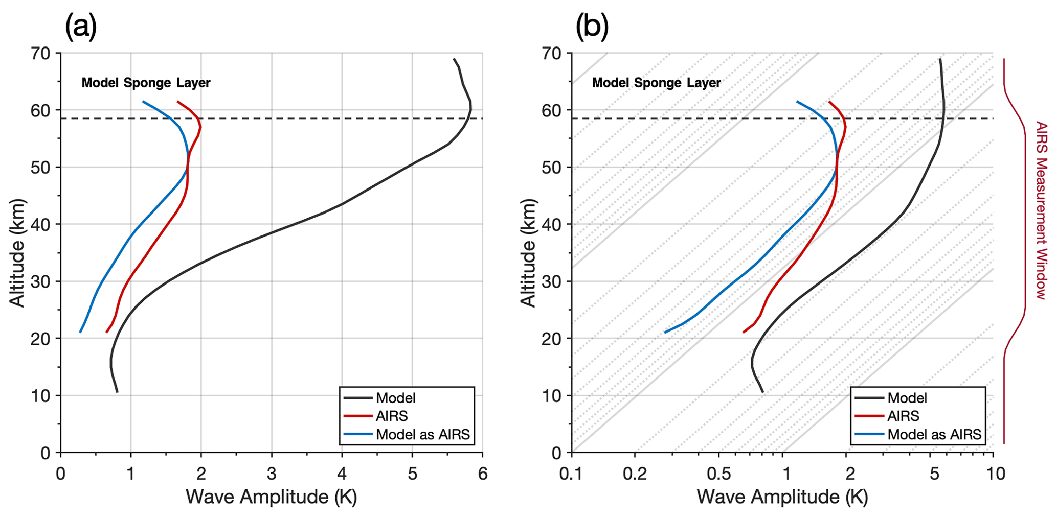
Figure 10 Vertical profiles of the average measured wave amplitudes over South Georgia in AIRS observations (red), the full-resolution model (black) and the model sampled as AIRS (blue) for June–July 2013 and 2015. Values are averaged over a horizontal area 600×400 km centred on the island (region C in Fig. 4). Both (a) and (b) show the same data, but in (b) the data are plotted on a logarithmic x axis where thin grey diagonal lines show the exponential adiabatic growth rate of GW amplitude with altitude $e^{\frac{z}{\mathrm{2}H}}$ expected from theory for an atmospheric scale height of H=7 km. The model damping “sponge” layer (dashed black line) begins at z=58.5 km and extends to the model top.

Average wave amplitudes in AIRS are up to 0.4 K larger than in the model sampled as AIRS at all altitudes up to around 45 km. As shown in Fig. 9a and e, this is likely due to larger GW amplitudes found at large distances from the island in AIRS, which increases the area average. Interestingly, however, although stratospheric GW amplitudes increase exponentially with altitude in all three datasets, but they appear to increase at different rates.

Figure 10b shows the same data as 10a but on a logarithmic amplitude scale. Between 25 and 45 km altitude, the model and the model sampled as AIRS closely follow the expected exponential adiabatic amplitude growth with height as $e^{\frac{z}{\mathrm{2}H}}$ (thin grey lines), where H=7 km is the approximate scale height of the atmosphere. Linear fits to the curves in Fig. 10b between altitudes of 25 and 45 km altitude yield gradients of 0.032 and 0.028 for the full-resolution model and the model sampled as AIRS respectively. These values are close to the gradient of around 0.031 (thin grey lines) that denotes theoretical exponential growth with height.

AIRS GW amplitudes, however, are found to increase more slowly with height. This is particularly evident even for altitudes between 25 and 35 km, despite the fact that this is where the AIRS vertical resolution is best (∼7–8 km; Hoffmann and Alexander, 2009). The amplitude growth rate in AIRS is the smallest over this height range. But this reduced growth rate is consistent with growth rates in GW potential energy during winter from limb-sounding observations as found by Wright et al. (2016b). A linear fit of the AIRS curve in Fig. 10b between 25 and 45 km altitude yields a gradient of 0.015, approximately half the growth rate found in the model. The fact that the model sampled as AIRS does not follow the same reduced growth rate as in the AIRS observations indicates that this difference is not likely to be due to changes in AIRS vertical resolution or retrieval noise with altitude. The reduced growth rate in AIRS could simply be because the scale height in the real atmosphere during this time period was greater than in the model, or it could indicate that some wave breaking, saturation or dissipation effects are not accurately simulated in the model. If the vertical resolution of our local-area model is too coarse, GWs are prevented from dissipating and would continue to increase in amplitude exponentially with altitude.

8 Large-amplitude mountain waves at short horizontal scales

In this section we consider GW measurements over the island at the very shortest horizontal scales visible to AIRS. Large-amplitude mountain waves are generally expected either directly above or just downwind of an orographic obstacle. The horizontal wavelength for the central region of a mountain wave field is primarily determined by the size of the obstacle in the direction of the prevailing wind, which is around 30–40 km for South Georgia. These large-amplitude and short-horizontal-wavelength waves can carry large momentum fluxes. In this section we show that, under favourable viewing conditions, AIRS can observe these waves.

Figure 11a–c shows AIRS, model and model-sampled-as-AIRS temperature measurements at 45 km altitude over South Georgia during an overpass at 17:00 UTC on 5 July 2015. As in Fig. 5, coloured circles indicate the location and extent of the AIRS measurement footprints. Alternating red–blue circles close to the island are indicative of large-amplitude GWs at the Nyquist sampling limit of the AIRS instrument, with a horizontal wavelength of around two AIRS footprints (∼27 km at nadir). Normally, we would be suspicious of such wave detections in AIRS measurements due to the retrieval noise, but the orientation of these features, their large magnitudes and their proximity to the island show close agreement with the expected mountain wave field in the full-resolution model.

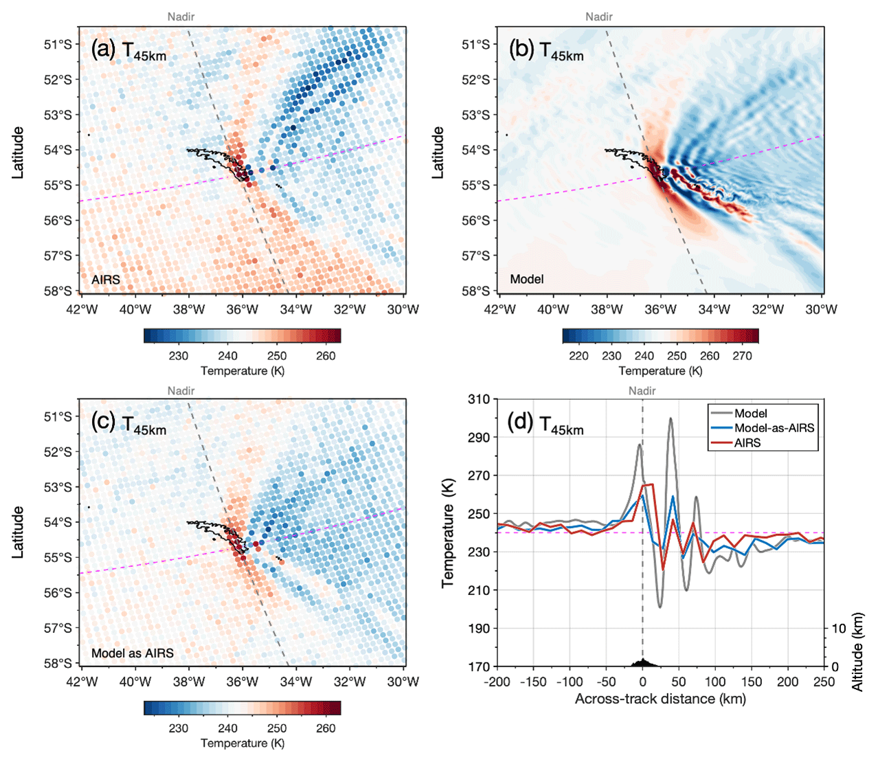
Figure 11 Temperature measurements over South Georgia at 45 km altitude at 17:00 UTC on 5 July 2015 for (a) AIRS satellite observations, the (b) full-resolution model and (c) the model sampled as AIRS. Coloured circles in (a) and (c) show the locations of the AIRS measurement footprints, while dashed grey lines show the satellite nadir, which passes directly over the island in this example. Panel (d) shows measured temperature at 45 km altitude against horizontal across-track distance along the dashed pink line in (a–c). Surface elevation along this path (right axes) is shown in black at the bottom of (d).

Inspection of the AIRS sampling pattern in Fig. 11a reveals three preferential conditions for the measurement of short-horizontal-scale mountain waves over South Georgia. Firstly, this overpass occurred during intense mountain wave activity in our study, as shown in Figs. 2 and 8. GWMF values near to this overpass are some of the largest measured during the time period studied here. Secondly, the nadir of the AIRS scan track passed directly over the island, as shown by the dashed grey line in Fig. 11a–c. The horizontal sampling between adjacent AIRS footprints is closest at nadir (∼13.5 km), which provides the best possible horizontal resolution for GWs.

Thirdly, we can see from Fig. 11a that the across-track scan direction is aligned perpendicular to the central section of the chevron-shaped mountain wave field, where the horizontal wavelengths are shortest. This means that these across-track rows, shown by the dashed pink line, bisect the mountain wave field perpendicular to the GW phase fronts in the central section of the mountain wave field, providing the most favourable viewing geometry for these short horizontal wavelengths. The orientation of the mountain wave field over the island, which is strongly related to the direction of the prevailing wind, does not always preferentially align with the across-track scan direction in such a way. For all the AIRS overpasses in our study that were inspected, only this example on 5 July 2015 showed such a clear alignment.

The full-resolution model in Fig. 11b exhibits a mountain wave field with fine-horizontal-scale structure. Short horizontal wavelengths near 30–40 km are found over and immediately downwind of the island, while turbulent eddies are apparent on the southern part of the mountain wave field. When the AIRS sampling and resolution is applied to the model, the mountain wave structure in panel c exhibits good qualitative agreement with the AIRS observations in panel a. As was shown in Fig. 6 above, the AIRS observations exhibit more mountain wave structure at larger horizontal distances to the north and south of the island.

We next take an across-track cut along the dashed pink line at 45 km altitude through all three datasets in Fig. 11a–c to show temperature against horizontal distance from the island in Fig. 11d. Because it is not straightforward to extract GW perturbations from model temperatures in the same way as the AIRS and the model sampled as AIRS, we present raw temperature measurements here to avoid any artefacts that may arise from inconsistent background removal methods for this example.

Temperatures rise and fall with increasing horizontal distance downwind of the island to the east in all three datasets with an apparent horizontal wavelength close to ∼30–40 km, and there is good agreement in GW phase. The full-resolution model exhibits large temperature perturbations of around ±45 K above and below the “background” temperatures of ∼245 K that are measured upwind of the island to the west. When the AIRS sampling and resolution are applied, the model sampled as AIRS exhibits perturbations close to ±15 K. These are in reasonable agreement with AIRS measurements, which exhibit temperature perturbations of around 15–20 K. Interestingly, positive perturbations in AIRS are larger than in the model sampled as AIRS in the first positive peak directly over the island but smaller in the second peak at around 40 km to the east. The third peak exhibits comparable perturbation amplitudes. This discrepancy could be caused by a slight offset in the position of the mountain wave structure in the model compared to observations or a slightly different horizontal wavelength, which could affect the measured wave amplitude when the AIRS sampling is applied to the model.

Several conclusions can be drawn from Fig. 11. Overall, the physical scale of observed and modelled mountain wave structures over the island shows good qualitative agreement for this example. The full-resolution model (1.5 km horizontal grid) indicates that the shortest characteristic horizontal wavelength of mountain waves directly over the island is around 30–40 km. When the AIRS sampling pattern is aligned preferentially, AIRS can resolve these short-horizontal-scale waves, as shown in AIRS measurements and in the model sampled as AIRS.

This is significant because the GW temperature perturbations over the island at these short horizontal wavelengths in this example are very large. If we had only found these waves in the model, we may ask the question of whether they could be supported in the real atmosphere. But because measured amplitudes in AIRS and the model sampled as AIRS show reasonable agreement, this suggests that the magnitude of wave amplitudes close to 45 K in the full-resolution model is realistic. These temperature perturbations of around ±45 K in the full-resolution model correspond to large horizontal and vertical wind perturbations near 45 km altitude of up to ±80 and ±60 m s⁻¹ respectively. To our knowledge, stratospheric GW temperature perturbations of this magnitude at such small horizontal scales are rarely seen in satellite observations. This is partly due to the limited observational filters of spaceborne instruments, but as we can see in Fig. 11, viewing geometry and horizontal sampling are also important.

Recent ground-based lidar observations austral during winter over the well-known GW hot spot of the Southern Andes by Kaifler et al. (2020) revealed GW temperature perturbations near ±40 K with vertical wavelengths around 16–18 km. Comparison with operational models in their study found good agreement between simulated and observed GWs. But the horizontal scale of the large-amplitude GWs measured by Kaifler et al. (2020) was close to λ_H≈400 km, which is around 10 times larger than we find over South Georgia in Fig. 11. This is an important result, because it suggests that the GWMF of such large-amplitude, short-λ_H waves over small mountainous islands can be very large and that high-resolution and favourable sampling is required in models and observations to simulate and measure this GWMF.

9 Discussion

9.1 Model sampled as AIRS: sensitivity to horizontal sampling and retrieval noise

One key process in this study is the application of the AIRS resolution and horizontal sampling to the model to create model-sampled-as-AIRS temperature perturbations that can be directly compared to AIRS observations. We found that our results were highly sensitive to the accuracy of this procedure. It is not enough to simply apply the horizontal and vertical resolutions of AIRS to the model; we must ensure that accurate horizontal sampling is also applied. This is because short-horizontal-scale (λ_H≲40 km) GWs directly over the island, which carry large momentum fluxes, are easily resolved on the model grid but are not always resolved in the AIRS observations due to limitations in sampling caused by inconsistent viewing geometry, as shown in Sect. 8. Therefore, if the AIRS horizontal sampling were not applied, the model sampled as AIRS would always overestimate these short-λ_H GWs compared to observations.

It is perhaps counterintuitive to apply unwanted retrieval noise to model output, but we found that this was also an essential step in our comparison. By applying the specified AIRS retrieval noise to the model sampled as AIRS, we can cancel out any effects of noise in our regional comparisons, specifically the comparison of upwind and downwind GW properties. Because GW temperature perturbations cannot always be separated from noise perturbations, the more retrieval noise that is present in measurements, the more even the distribution of GWMF between the upwind and downwind regions in Table 1. If we did not apply retrieval noise to the model sampled as AIRS, a fair comparison would not be possible.

We should note, however, that the specified retrieval noise that we applied is randomised to uncorrelated pixel-scale noise for each altitude level, so if there are elements of retrieval noise in AIRS measurements that have larger horizontal scales greater than around 30–50 km, these may not be correctly applied to the model sampled as AIRS.

9.2 Simulation of NGWs in the local-area model

In Sect. 7.2 we found that, compared to the AIRS observations, the model sampled as AIRS may underestimate NGW wave activity at large horizontal distances from the island, particularly upwind. This is significant because de la Cámara et al. (2016) recently showed that an even balance between orographic and NGW parameterisations near 60^∘ S had a significant impact on reducing the cold-pole biases. They found that sporadic large-amplitude NGW parameterisations from specific sources provide greater forcing on the circulations than a homogeneous distribution of NGW parameterisations.

Hindley et al. (2019, their Fig. 1) reported that sporadic large-amplitude NGWs can often be found in AIRS observations around the Southern Ocean during winter. We also find suggestions of such waves in our Fig. 5a, so their apparent underestimation in our local-area model is important. As discussed in Sect. 6, the global forecast that supplies the lateral and initial boundary conditions for the local-area model has a coarser vertical and horizontal resolution, with only 70 vertical levels from the surface to near 80 km and a horizontal grid spacing close to 60 km at latitudes near South Georgia. Even if NGWs are realistically simulated in the global forecast, it is not clear how well these waves would be “transmitted” through the interface between the global forecast and the local-area model. Further, the time integration used between the global forecast and the local-area model time step may further invalidate the realism of any transferred waves. As a result, non-stationary NGWs generated outside the local-area model, such as those from storms, jets, fronts and geostrophic adjustment processes, are unlikely to be realistically simulated in the local-area model. This is a consequence of the nested model configuration used here, which is designed to produce realistic wind conditions over South Georgia for mountain wave generation. If the horizontal extent of the local-area simulation and the number of vertical levels in the global forecast are increased, we would expect that transitory NGWs would be better simulated in the local-area model.

It is also important to note that it is not just model resolution which is important for accurate gravity wave simulations. Model numerics can also be significant. The Met Office Unified Model used here uses semi-implicit time integration for operational efficiency, but choosing too large a time step can make the model dissipative to GWs (e.g. Shutts and Vosper, 2011; Vosper, 2015), which could lead to an underestimation of gravity wave amplitudes. However, time-averaged GW amplitudes directly over the island in Fig. 9 appear to show a reasonable agreement between AIRS and the model sampled as AIRS, suggesting that this effect is small for mountain waves, which have ground-based horizontal phase speeds close to zero.

9.3 Large-amplitude mountain waves directly over the island

In Sect. 8 we found good agreement between the AIRS and the model sampled as AIRS for the shortest characteristic horizontal wavelengths around 30–40 km for mountain waves directly over South Georgia. Here, these waves have large amplitudes up to 20 K in AIRS measurements and can carry large momentum fluxes.

But these GWs at short horizontal wavelengths lie at the sampling and resolution limits of AIRS measurements. They are only visible in Fig. 11 due to the favourable viewing geometry of this specific AIRS overpass, where the satellite nadir passes directly over the island and the across-track direction is aligned parallel (perpendicular) to the background wind vector (GW phase fronts). Because these conditions are not the same for each overpass, this means that the GWMF from these large-amplitude, short-λ_H waves may be underestimated in recent AIRS GWMF climatologies (Hindley et al., 2020). This underscores the importance of considering how instrument sampling patterns contribute to the observational filters of spaceborne GW measurements and further highlights that future comparisons between models and observations should consider both horizontal sampling and resolution (Wright and Hindley, 2018).

10 Summary and conclusions

In this study, we compare simulated stratospheric gravity waves (GWs) over the small mountainous island of South Georgia to coincident 3-D AIRS satellite observations. Such islands currently lie in the grey zone of global model resolution, where they are neither fully resolved nor fully parameterised (Vosper, 2015; Vosper et al., 2016). Thus, critically assessing simulated GW momentum fluxes generated by these islands is crucial for the development of accurate future global models.

We use a local-area model configuration with a high spatial resolution (1.5 km horizontal grid, 118 vertical levels) that can resolve the mountainous orography of the island and accurately simulate mountain wave generation and propagation. We apply the sampling and resolution of AIRS to the model to create a model-sampled-as-AIRS dataset. This allows us to make direct like-for-like comparisons of simulated and observed GW amplitudes, wavelengths and directional momentum fluxes during two periods in July 2013 and June–July 2015. We find the following:

1. The timing of GW activity in the local-area model generally agrees well with the AIRS observations. This suggests that mountain wave forcing, propagation and background winds in the model are accurately simulated to first order and that the 1.5 km horizontal grid is sufficient to generate realistic stratospheric mountain waves.

2. When the model is sampled as AIRS, good agreement is found in net GW momentum flux (GWMF) over the island. Average zonal (meridional) GWMF over this 2-month period is westward (southward) at 5.3 (2.7) and 5.6 mPa (−2.2 mPa) in AIRS and the model sampled as AIRS respectively.

3. Both peak and area-averaged GW amplitudes in the model sampled as AIRS are ∼20 %–30 % smaller than seen in AIRS. Upwind of the island, 35 % of the total GWMF is found in AIRS compared to only 17 % in the model sampled as AIRS. This suggests that although the model configuration used here simulates realistic orographic GWMF over the island, it underestimates non-orographic GW activity over the surrounding ocean.

4. Average GW amplitudes in AIRS, but not the model sampled as AIRS, are found to increase more slowly with height than expected from theory. This could be because simulated wave breaking or dissipation processes in the model are incomplete, either due to insufficient vertical grid spacing or underrepresented wave–wave or wave–mean-flow interactions.

5. An ∼20 % northward bias in meridional GWMF is found in the model sampled as AIRS. This bias could be related to, or even caused by, a large southward wind bias of up to 10 m s⁻¹ in the model compared to coincident radiosonde observations at altitudes above ∼10 km.

6. Finally, AIRS measurements reveal large-amplitude ($T^{\prime }\approx \mathrm{15}$–20 K at 45 km altitude) mountain waves with λ_H≈30–40 km directly over the island. These waves are at the shortest horizontal scales visible to AIRS, and they are only detectable due to favourable viewing geometry during one specific overpass. AIRS-measured λ_H and T^′ for this example show excellent agreement with the model sampled as AIRS. This example provides valuable experimental evidence that large-amplitude (up to $T^{\prime }\approx \mathrm{45}$ K at 45 km altitude) short horizontal wavelength (λ_H≈30–40 km) mountain waves, as seen in the full-resolution model here, are physical and can occur in the real atmosphere.

Despite the increasing availability of global GW observations in recent years, direct comparisons of GWs in observations and models have been limited by several fundamental factors, including (a) the observational filter problem, (b) a lack of the 3-D observations needed to constrain the directionality of GW momentum fluxes, (c) insufficient model resolution to accurately resolve small-scale GWs and (d) the need for realistic background wind conditions for specific time periods for dedicated high-resolution offline simulations.

In this study, we have overcome each of these obstacles to make accurate and detailed comparisons between observed and simulated GWs over the mountainous island of South Georgia. We find that, for a high-resolution real-time simulation that is guided by a global forecast, good agreement can be found between simulated wintertime GWs and coincident 3-D GW observations if the observational filter of the instrument is carefully applied to the model. In particular, we show that when the sampling pattern is orientated favourably with respect to the wave, agreement between GWs in AIRS observations and the model can be excellent.

However, some important biases do remain between the model and the observations. Specifically, our model configuration exhibits directional biases and underestimates non-orographic GW activity in the region compared to observations. These discrepancies likely arise from the nested local-area configuration used here, and they may be greatly reduced in a global model operating at this spatial resolution. As such models become available in the future, our study points to an effective way forward for future comparisons of GWs in high-resolution models and observations.