the Creative Commons Attribution 4.0 License.
the Creative Commons Attribution 4.0 License.
 | 20 May 2021
Time-dependent 3D simulations of tropospheric ozone depletion events in the Arctic spring using the Weather Research and Forecasting model coupled with Chemistry (WRF-Chem)
Maximilian Herrmann
Holger Sihler
Udo Frieß
Thomas Wagner
Ulrich Platt
Eva Gutheil
Tropospheric bromine release and ozone depletion events (ODEs) as they commonly occur in the Arctic spring are studied using a regional model based on the open-source software package Weather Research and Forecasting model coupled with Chemistry (WRF-Chem). For this purpose, the MOZART (Model for Ozone and Related chemical Tracers)–MOSAIC (Model for Simulating Aerosol Interactions and Chemistry) chemical reaction mechanism is extended by bromine and chlorine reactions as well as an emission mechanism for reactive bromine via heterogeneous reactions on snow surfaces. The simulation domain covers an area of 5040 km×4960 km, centered north of Utqiaġvik (formerly Barrow), Alaska, and the time interval from February through May 2009. Several simulations for different strengths of the bromine emission are conducted and evaluated by comparison with in situ and ozone sonde measurements of ozone mixing ratios as well as by comparison with tropospheric BrO vertical column densities (VCDs) from the Global Ozone Monitoring Experiment-2 (GOME-2) satellite instrument. The base bromine emission scheme includes the direct emission of bromine due to bromide oxidation by ozone. Results of simulations with the base emission rate agree well with the observations; however, a simulation with 50 % faster emissions performs somewhat better. The bromine emission due to bromide oxidation by ozone is found to be important to provide an initial seed for the bromine explosion. Bromine release due to N2O5 was found to be important from February to mid March but irrelevant thereafter. A comparison of modeled BrO with in situ and multi-axis differential optical absorption spectroscopy (MAX-DOAS) data hints at missing bromine release and recycling mechanisms on land or near coasts. A consideration of halogen chemistry substantially improves the prediction of the ozone mixing ratio with respect to the observations. Meteorological nudging is essential for a good prediction of ODEs over the 3-month period.
- Article
(20924 KB) - Full-text XML
- Companion paper
-
Supplement
(9099 KB) - BibTeX
- EndNote


Ozone is an important constituent of the troposphere due to its high oxidation potential. In the Arctic troposphere, ozone mainly originates from transport and photochemical reactions involving nitrogen oxides and volatile organic compounds, resulting in a background mixing ratio of 30 to 50 nmol mol−1 (ppb). During polar spring, so-called tropospheric ozone depletion events (ODEs) are regularly observed, in which ozone mixing ratios in the boundary layer drop to almost zero levels coinciding with a surge in reactive bromine levels on a timescale of hours to days (e.g., Oltmans, 1981; Bottenheim et al., 1986; Barrie et al., 1988; Hausmann and Platt, 1994; Wagner and Platt, 1998; Frieß et al., 2004; Wagner et al., 2007; Helmig et al., 2012; Halfacre et al., 2014). ODEs strongly shorten the lifetime of ozone and organic gases, they cause the removal and deposition of mercury as well as the transport of reactive bromine into the free troposphere. During an ODE, ozone is destroyed by Br atoms in the catalytic reaction cycle (e.g., Barrie et al., 1988; S. Wang et al., 2019)
resulting in the following net reaction:
The rate-limiting reaction in this cycle is usually the BrO self-reaction (R2) with a reaction rate that is quadratic in the BrO concentration. The source of the reactive bromine is thought to be sea salt, i.e., aerosol, which deposits on the snow (Fan and Jacob, 1992; McConnell et al., 1992; Platt and Janssen, 1995; Pratt et al., 2013; Simpson et al., 2015; Custard et al., 2017). However, it is not fully understood how the salt bromide is oxidized and how the reactive bromine is released into the air. The most widely accepted emission mechanism is autocatalytic and termed “bromine explosion” (Platt and Janssen, 1995; Platt and Lehrer, 1997; Wennberg, 1999), which consists of the Reactions (R1) and (R3) and the following two Reactions (R5) and (R6):
Reaction (R6) is a heterogeneous reaction, i.e., a reaction involving gaseous components (HOBr) and liquid-phase components (H+ and Br−). The concentration of atomic gas-phase bromine doubles in each reaction cycle as can be seen in the following net reaction:
Since H+ ions are consumed, it implies the need for acidic solutions for this reaction to occur, and a pH of at most 6.5 is suggested by Fickert et al. (1999) for this reaction to occur efficiently. A pH dependence of the Br2 production was shown by Pratt et al. (2013) through field-based experiments and by Wren et al. (2013) and Halfacre et al. (2019) through lab-based experiments.
Other pathways to activate bromide were suggested, involving nitrogen oxides,
as well as a direct emission due to bromide oxidation by ozone (e.g., Oum et al., 1998; Artiglia et al., 2017), which are likely to need sunlight to efficiently occur (Pratt et al., 2013):
In the following discussion, the term bromine explosion mechanism includes the original Reactions (R1), (R3), (R5), and (R6) as well as Reaction (R9), which also generates two bromine atoms out of one gas-phase bromine atom and represents an extended bromine explosion mechanism. Reaction (R10) is considered independently of this terminology as bromide oxidation due to ozone.
A further Br2 release mechanism initiated by a reaction of the hydroxyl radical OH with bromide inside the surface layer of the snow grains under sunlight was suggested (Sjostedt and Abbatt, 2008; Pratt et al., 2013). Evidence for this mechanism was found in a laboratory study (Halfacre et al., 2019). The release mechanism may be summarized in the net reaction
A consequence of the reduced ozone levels during an ODE is that reactions of reactive bromine with OH or certain organic species producing chemically inert HBr are favored (essentially reactive bromine is returned to the bromide reservoir), e.g.,
HBr then deposits into the ground or onto aerosols, ultimately terminating the ODE. Chlorine and iodine play a smaller role for the occurrence of ODEs (Thompson et al., 2015). The reaction of methane with chlorine atoms quickly produces chemically inert HCl. Since Cl atoms react with CH4 (while Br and I atoms do not) and due to the large abundance of methane in the atmosphere, chlorine explosions cannot occur in the atmosphere. The iodine concentration (I− and ) is approximately 20 times smaller than bromide in seawater (Luther et al., 1988; Grebel et al., 2010), which is likely the reason why detectable amounts of gaseous iodine have been rarely found in the Arctic and the Antarctic (Wittrock et al., 2000; Schönhardt et al., 2008; Saiz-Lopez et al., 2007; Atkinson et al., 2012; Zielcke, 2015; Raso et al., 2017). Both iodine and chlorine, however, may still play a role due to inter-halogen reactions:
with X=Cl or I, which occur faster by an order of magnitude (Atkinson et al., 2007) than the BrO self-reaction (R2).
Similarly, chloride can speed up bromine activation (Simpson et al., 2007a):
aqueous BrCl can further be converted into Br2:
ODEs are observed mostly in the polar spring. During winter, radical bromine chemistry cannot occur due to the lack of sunlight. Temperatures below −20 ∘C are likely to favor the occurrence of ODEs (Tarasick and Bottenheim, 2002; Pöhler et al., 2010). However, Bottenheim et al. (2009) observed ODEs at −6 ∘C and Halfacre et al. (2014) found no apparent temperature dependence for the presence of an ODE in ozone measurements at five buoys across the Arctic. Shallow boundary layers are also likely to be beneficial (Wagner et al., 2001; Frieß et al., 2004; Lehrer et al., 2004; Koo et al., 2012), since they increase the speed of the autocatalytic bromine release by confining the released bromine to a smaller space. The age of the sea ice is also an important factor. Snow covering first-year (FY) ice, which has more accessible salt than multi-year (MY) ice, is expected to be the main source of bromine (Simpson et al., 2007b; Abbatt et al., 2012). Despite being often depleted in bromide, snow covering MY ice may still play an active role in the release of reactive bromine (Peterson et al., 2019). Pratt et al. (2013) did not directly observe Br2 emissions from the sea ice, which is likely due to a higher pH of the sea ice due to buffering (Wren and Donaldson, 2012). ODEs are much less pronounced in polar fall with rare measurements of partial ODEs in the Antarctic (Nasse, 2019) because most of the brine covering FY ice will have drained away during the summer melt (Simpson et al., 2007b) even though meteorological conditions are similar to those in spring time.
Snow covering land surfaces may also play an active role in the release of Br2, as several studies suggest (Simpson et al., 2005; Peterson et al., 2018). Custard et al. (2017) simultaneously measured Br2, BrCl, and Cl2 in the snowpack interstitial air and also provided estimates of Br2 and Cl2 emission rates. McNamara et al. (2020) measured the release of BrCl from snow surfaces, and the dominant pathways of BrCl were identified in a box model simulation. Thomas et al. (2011) extended the 1D model called MISTRA with a snowpack module and validated their results with observations at Summit, Greenland. They found the solar actinic flux to be the main driver of reactive bromine release from the liquid-like layer (LLL) of the snow grain surface and a dependence of bromine release from the LLL on the OH concentration in the LLL. Wang and Pratt (2017) attributed approximately 20 % of the total Br2 production to the mechanism of snow Br2 production. S. Wang et al. (2019) measured atomic bromine and related it to BrO and snow-released Br2, finding 3 to 10 times higher levels of atomic bromine than previous estimates suggested.
From the outline above it is clear that ODEs are a complex function of chemistry and meteorology; therefore, 3D simulations are useful to learn about the interaction of meteorology and chemistry in generating ODEs. Earlier studies estimated boundary layer BrO from measurements of satellite BrO vertical column densities (VCDs) (e.g., Wagner and Platt, 1998; Zhao et al., 2008) by estimating the BrO release from sea-salt aerosols produced from abraded frost flowers (Kaleschke et al., 2004; Zhao et al., 2008) or from blowing-snow events (Yang et al., 2008, 2010). Toyota et al. (2011) reproduced major features of satellite BrO VCDs and in situ measurements using a simple parameterization of bromine emissions from bulk ice and snow with the 3D air quality model Global Environmental Multiscale model with Air Quality processes (GEM-AQ). Falk and Sinnhuber (2018) integrated this mechanism into the ECHAM/MESSy Atmospheric Chemistry (EMAC) model, investigating and reproducing important features of ODEs for a full annual cycle.
In the present study, the regional 3D online numerical weather prediction system Weather Research and Forecasting model coupled with Chemistry (WRF-Chem) is used to investigate the ODEs during Arctic spring from 1 February through 1 May 2009 since for this period of time, extensive data from observations are available from the National Oceanic and Atmospheric Administration (NOAA) institute or collected as part of the Ocean–Atmosphere Sea-Ice Snowpack (OASIS) field initiative for comparison with the numerical results. The chemical reaction scheme MOZART (Model for Ozone and Related chemical Tracers)–MOSAIC (Model for Simulating Aerosol Interactions and Chemistry) is extended by bromine and chlorine reactions to study their impact on the ODEs. The emission scheme developed by Toyota et al. (2011) is adopted and a parameter study for the reactive surface ratio (Cao et al., 2014) of the ice or snow surface is performed.
First, the configuration of WRF-Chem (Grell et al., 2005; Skamarock et al., 2008) will be presented, then the modifications to the standard configuration will be discussed and the initial and boundary conditions will be provided.
2.1 Configuration of WRF-Chem
The physical area (displayed in Fig. 1) of 5040 km×4960 km, centered north of Utqiaġvik is modeled for the time interval of 1 February through 1 May 2009, for which Global Ozone Monitoring Experiment-2 (GOME-2) data with a stratospheric correction for BrO VCDs (Sihler et al., 2012) as well as surface ozone and ozone sonde data are available for model evaluation.

Figure 1Domain of the simulations presented in this publication and sea ice type (Aaboe et al., 2017) with the locations of (•) Utqiaġvik, Alaska, and (⧫) Summit, Greenland, respectively. For latitudes larger than 88∘, missing sea ice type data are filled up with FY ice. The horizontal line refers to the x coordinate in Fig. 6.
Table 1Summary of the configuration of WRF-Chem. RRTMG refers to the Rapid Radiative Transfer Model for GCMs (global circulation models), LW stands for longwave, SW stands for shortwave, WSM denotes WRF Single Moment, TUV stands for Tropospheric Ultraviolet and Visible, EDGAR-HTAP stands for Emissions Database for Global Atmospheric Research – Hemispheric Transport of Air Pollution, and MEGAN stands for Model of Emissions of Gases and Aerosols from Nature.
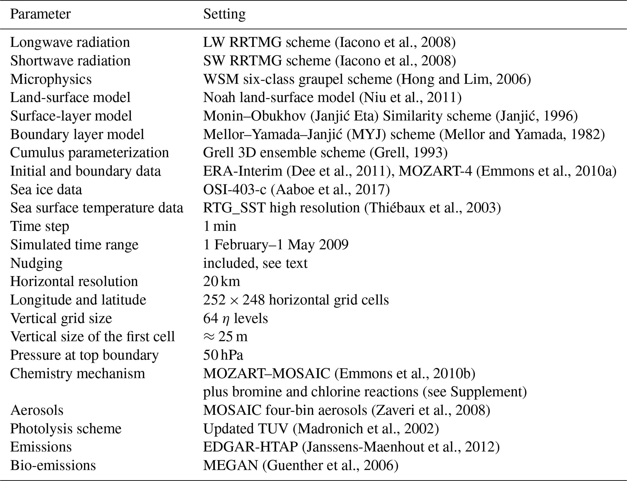
The software Weather Research and Forecasting model coupled with Chemistry (WRF-Chem) version 3.9 is employed. WRF-Chem (Skamarock et al., 2008; Grell et al., 2005) is a state-of-the-art regional numerical weather prediction system with online computation of chemistry. Table 1 summarizes the configuration of the software. The physics modules are chosen following recommendations of the polar WRF community (Bromwich et al., 2009, 2013; Wilson et al., 2011); the modules include the meteorology and the emission, transport, mixing, and chemical reactions of trace gases as well as aerosols.
The simulation domain is centered north of Utqiaġvik using the polar stereographic projection at a true latitude of 83∘ with a reference longitude of 156∘ W. A horizontal grid resolution of 20 km for the 5040 km×4960 km domain is employed, allowing a comparison to GOME-2 BrO satellite data (Sihler et al., 2012) with a resolution of approximately 40 km×30 km. In the vertical direction, 64 non-equidistant grid cells with a finer resolution near the ground are used, starting with approximately 25 m at the ground level. Half of the grid cells used in the present study are in the first 2 km of the atmosphere, allowing a detailed representation of the Arctic boundary layer. The vertical grid is provided in the Supplement of this paper.
The meteorological time step of 1 min is chosen to fulfill the Courant criterion. Chemistry is updated between every meteorology time step, and radiative transfer is updated every 10th meteorological time step.
In the present model, the Mellor–Yamada–Janjić (MYJ) planetary boundary layer (PBL) scheme (Mellor and Yamada, 1982; Janjić, 1990) is employed, which is a 1.5-order local turbulence closure model. Prognostically determined turbulent kinetic energy is used to determine the eddy diffusion coefficients. The MYJ PBL scheme is best suited for stable to slightly unstable conditions (Mellor and Yamada, 1982).
2.2 Gas-phase chemistry
WRF-Chem offers several implementations of chemical reaction schemes. In the present study, the MOZART–MOSAIC mechanism based on MOZART-4 gas-phase chemistry (Emmons et al., 2010a) is used, which includes 85 gas-phase species, 237 gas-phase reactions, and 49 photolysis reactions. An additional 18 gas-phase species, 73 gas-phase reactions, and 13 photolysis reactions (Herrmann et al., 2019) account for the bromine and chlorine chemistry (termed “full chemistry”, see Table 2). Observations of reactive iodine in the Arctic region (Zielcke, 2015; Raso et al., 2017) suggest only low mixing ratios of iodine. Even though small mixing ratios of iodine can significantly enhance ozone depletion (Raso et al., 2017), iodine is neglected due to the uncertainties in the abundance of iodine in the Arctic atmosphere and in snowpacks. The photolysis rates are calculated with the “Updated TUV” (Tropospheric Ultraviolet–Visible) scheme (Madronich et al., 2002), which already contains the halogen photolysis reaction rates. The added bromine and chlorine chemical reactions are provided in the Supplement.
2.3 Aerosol-phase chemistry
The MOZART–MOSAIC mechanism employs four-bin MOSAIC aerosols (Zaveri et al., 2008). In WRF-Chem, MOSAIC is implemented using a sectional approach, where size bins are defined by the upper and lower dry particle diameters. In MOSAIC, the mass and number density for each bin are considered, and the processes of nucleation, coagulation, condensation, evaporation, and aerosol chemistry are modeled. The mass transfer rate ki,m for gas species i and aerosol size section m is calculated using the following parameterization (Wexler and Seinfeld, 1991):
where Dg,i is the gas diffusivity of species i, Rp,m is the wet mean particle radius of size bin m, Nm the number density of size bin m, and is the Knudsen number of size bin m with the free mean path λ. f(Knm,γi) is the transition regime correction factor (Fuchs and Sutugin, 1971) and accounts for the interfacial mass transport limitation:
where γi is the accommodation coefficient for gas-phase species i taken from the CAABA/MECCA (Chemistry As A Boxmodel Application/Module Efficiently Calculating the Chemistry of the Atmosphere) model (Sander et al., 2011). Aerosol forms of bromine are currently not implemented in the MOSAIC framework and are treated as gas-phase species. The transfer reactions of bromine gas-phase species X to aerosol-size bin m are assumed to produce species Xaq,m as
which may produce gas-phase Br2 (McConnell et al., 1992; Peterson et al., 2017):
Reactions (R17)–(R20) may only occur if the aerosol is in a liquid state, and, in addition, Reaction (R20) requires the aerosol to have a pH of 6 or less. The heterogeneous reactions and parameters required to calculate the reaction rates are listed in the Supplement. Heterogeneous BrCl production (Reactions R15 and R16) is not implemented in the model.
2.4 Bromine emission scheme
Emissions of bromine species on snow surfaces are parameterized following Toyota et al. (2011). Numerically, bromine emissions are coupled to vertical diffusion. In WRF-Chem, vertical (turbulent) diffusion for each species and horizontal grid cell is solved using a Peaceman–Rachford alternating direction implicit method (Peaceman and Rachford, 1955). The bromine emissions are added as boundary conditions to the tridiagonal diffusion matrix. For the surface emission in Reactions (R6), (R9), and (R10), the boundary flux for instance of Reaction (R6), Fd(Br2|HOBr) for Br2 due to HOBr is
where ρd,0 is the dry air density of the lowest grid cell and [HOBr]0 is the HOBr mixing ratio in the lowest grid cell. The species-dependent deposition velocity vd≈1 cm s−1 is calculated using the WRF-Chem Wesely deposition module (Wesely, 1989) under an additional assumption of near-zero surface resistance. Thus, the turbulent transfer resistance dominates the deposition velocity, and the bromine emissions increase with larger wind speeds. β≥1.0 is the reactive surface ratio (Cao et al., 2014) of the ice or snow surface, accounting for non-flat surfaces such as ice or snow and frost flowers. For simplicity, β is set as a global value in this study to allow for the investigation of the strength of bromine emissions in a parameter study. For the direct emission of bromine due to ozone oxidation of bromide (see Reaction R10 above), the factor α is used to control the emission probability:
and
The value of α is parameterized with a dependence on the solar zenith angle (SZA) (Toyota et al., 2011):
The deposition velocity for ozone is dominated by the surface resistance (Wesely, 1989), leading to vd(O3)≈0.01 cm s−1. An emission mechanism relating to the bromide oxidation by the hydroxyl radical (see Reaction R11) is currently not implemented in the model. All sea ice is assumed to be snow covered for the simulated time range. On snow covering FY ice, it is assumed that the bromide content is infinite, so that unrestricted gaseous bromine emissions are possible, and emissions of Br2 due to O3 and N2O5 depositions are only active on snow covering FY ice. On snow covering MY ice, no bromide content but infinite chlorine is assumed. HOBr depositions only release Br2 up to the combined depositions of gaseous and aerosol HBr, whereas excess HOBr depositions release BrCl. On snow-covered land, neither bromide nor chloride content is assumed, so that excess HOBr depositions are lost. A list of the depositions and emissions added to the MOZART mechanism can be found in the Supplement. Br2 production from the sunlit condensed phase without any depositions of gas-phase species as found under certain conditions by Pratt et al. (2013) and Halfacre et al. (2019) as well as possible oceanic emissions of very short-lived brominated species are currently not considered in the model.
2.5 Initial and boundary conditions
ERA-Interim (Dee et al., 2011) is used to generate both the initial and boundary meteorological and sea ice cover data. ERA-Interim was found to perform well in polar regions in various studies (e.g., Bracegirdle and Marshall, 2012; Bromwich et al., 2016) and was successfully used in various modeling studies in polar regions (e.g., Hines et al., 2015; Cai et al., 2018), which is why it was chosen in the present study. Nudging of temperature, horizontal wind speed, humidity, and surface fields to ERA-Interim data ensures the validity of the simulation meteorology over the simulated 3-month period. The idea of the present work is not to try to make meteorological predictions (which would not be meaningful anyway on the timescale of a few months) but rather to model chemistry under meteorological conditions prevailing over a particular period of time. Nudging is active for the entire duration of the simulation and is inactive inside the boundary layer. The nudging timescale is set to 1 h. MOZART-4 results driven by Goddard Earth Observing System (GEOS-5) meteorological fields are used as initial and boundary data for all non-halogen species (Emmons et al., 2010a). For most halogen species, initial and boundary conditions are set to near-zero values. The initial mixing ratio of HBr and Br2 is set to 0.3 ppt in the lowest 200 m of the atmosphere. The mixing ratio of CHBr3 is fixed to 3.5 ppt (Toyota et al., 2014). The bromide oxidation of ozone in the dark for an ozone deposition velocity of 0.01 cm s−1, a boundary layer height of 200 m, an emission probability of Φ=0.001, and 40 nmol mol−1 ozone will release approximately 2 pmol mol−1 Br2 on FY ice per day. This emission rate is assumed to prevail for all simulations with active halogen chemistry. The chosen initial halogen concentrations and the fixed mixing ratio of CHBr3 are thus irrelevant. The RTG_SST (where RTG stands for real-time global) high-resolution dataset (Thiébaux et al., 2003) is used for the sea surface temperature (SST). The present model differentiates between FY and MY sea ice in order to estimate bromine emissions. For this purpose, the OSI-403-c (where OSI stands for ocean and sea ice) sea ice type dataset (Aaboe et al., 2017) is used. The original dataset does not provide values for latitudes larger than about 88∘ due to a lack of satellite measurements for these latitudes. In the present study, these values are filled with first-year sea ice. Figure 1 shows the simulation domain and the locations of FY and MY sea ice. Grid cells with a mixed FY–MY sea ice type are treated as multi-year sea ice in the bromine emission mechanism described above. Sea ice cover, SST, and sea ice type are updated online during the numerical simulations. EDGAR-HTAP (Janssens-Maenhout et al., 2012) and MEGAN (Guenther et al., 2006) are used as anthropogenic emissions and bio-emissions, respectively.
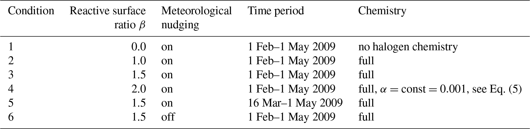
2.6 Conducted simulations and observations for comparison
The conducted simulations are summarized in Table 2. Five different observational datasets are used for comparison to the simulation results:
-
ground-based in situ ozone measurements at Utqiaġvik, Alaska, and Summit, Greenland (McClure-Begley et al., 2014);
-
ground-based in situ BrO measurements at Utqiaġvik, Alaska (Liao et al., 2012);
-
vertical profiles of the ozone mixing ratio derived from ozone sonde measurements at Utqiaġvik (Oltmans et al., 2012);
-
vertical profiles of the BrO mixing ratio derived from multi-axis differential optical absorption spectroscopy (MAX-DOAS) measurements at Utqiaġvik (Frieß et al., 2011);
-
maps of vertical BrO column densities from GOME-2 satellite measurements (Sihler et al., 2012).
For comparison of the observations and the simulations, three different statistical parameters are used. For model variable M and the corresponding observation variable O, the Pearson correlation R, the mean bias MB, and the root mean square error RMSE are calculated by
where 〈〉 is the mean and σM and σO denote the standard deviations of M and O, respectively.
2.6.1 Retrieval of the tropospheric BrO VCD from GOME-2 observations
The tropospheric BrO vertical column density (VCD) is derived from GOME-2 observations as described in detail by Sihler et al. (2012). GOME-2 is a UV–visible or near-IR spectrometer with moderate spectral resolution aboard the Meteorological Operational (MetOp) satellite (Callies et al., 2000; Munro et al., 2006, e.g.,), which was launched in 2006. With a swath width of 1920 km, almost global coverage is achieved every day. In polar regions, the same location is observed several times during 1 d. The ground pixel size is approximately 80 km×40 km.
The atmospheric BrO absorption is analyzed in the spectral range from 336–360 nm. In order to obtain the tropospheric BrO column, the stratospheric BrO column is estimated using the simultaneously retrieved stratospheric columns of O3 and NO2. In the final step, the retrieved tropospheric BrO slant column density (SCD) is converted into the tropospheric BrO VCD using simultaneous measurements of O4 and the radiance at 372 nm. Finally, the retrieved BrO VCDs are filtered and only measurements above a chosen sensitivity threshold of 0.5 for the air mass factor (AMF) of the lowest 500 m are used. More details on the data analysis are provided by Sihler et al. (2012)
2.6.2 Retrieval of BrO vertical profiles from MAX-DOAS
Vertical profiles of BrO are derived from MAX-DOAS measurements during the OASIS campaign at Utqiaġvik between February to April 2009 as described by Frieß et al. (2011). In brief, BrO and aerosol profiles are retrieved on vertical layers of 100 m thickness in the lowermost 2 km of the atmosphere with a temporal resolution of 15 min using the HEIPRO (Heidelberg PROfile) retrieval algorithm (Frieß et al., 2019). HEIPRO is based on the well-established optimal estimation method (Rodgers, 2000), with SCDs of atmospheric trace gases observed at different elevation angles serving as measurement vector. In a first step, aerosol extinction vertical profiles are determined using the observed optical thickness of the oxygen collision complex O4 as a proxy for the atmospheric light path (Frieß et al., 2006). In a second step, BrO vertical profiles are retrieved using BrO slant column densities, together with the aerosol extinction profiles retrieved in the first step. The limited information content of MAX-DOAS measurements requires the usage of appropriate a priori aerosol and BrO vertical profiles as described in Frieß et al. (2011). Averaging kernels quantify the sensitivity of the retrieved profile to the true profile x. In order to account for the limited vertical resolution of MAX-DOAS measurements and to allow for a quantitative comparison of model and measurement, modeled vertical profiles are convoluted with the MAX-DOAS averaging kernels according to Rodgers and Connor (2003):
Here, xm is the modeled and xa the a priori BrO profile. It is important to note that the vertical sensitivity strongly depends on visibility that varied strongly during the OASIS campaign due to frequent storms with blowing snow.
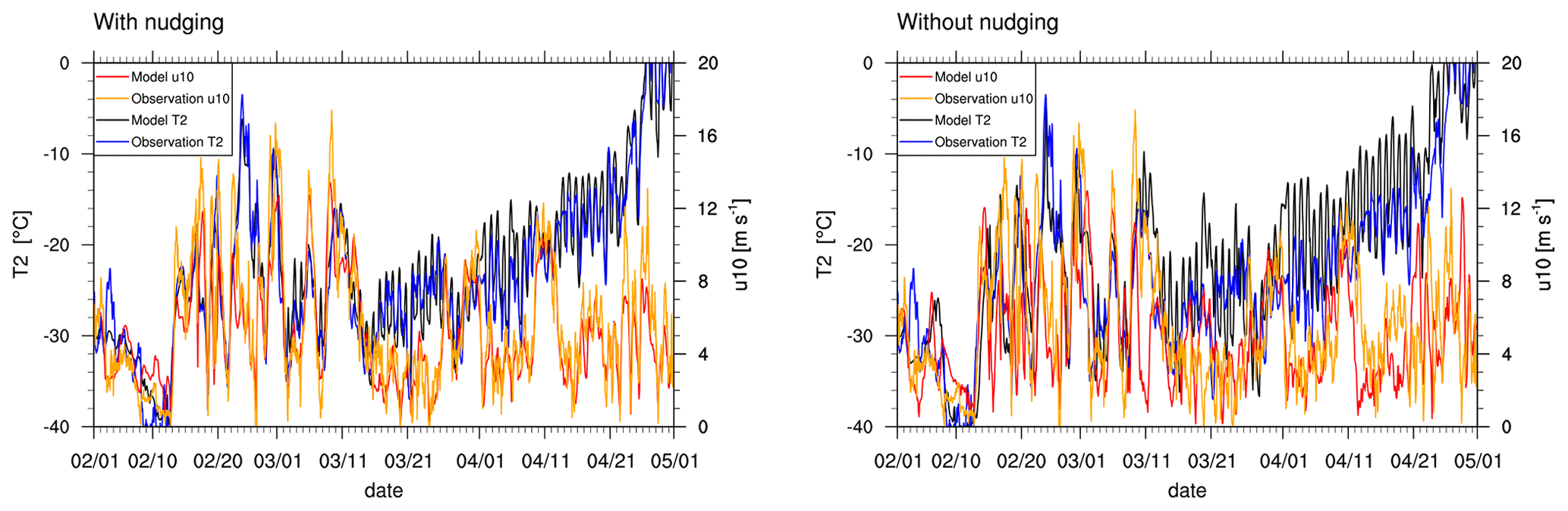
Figure 2Profiles of 2 m temperature and 10 m wind speed at Utqiaġvik in February through May 2009. The data are shown at 06:00 GMT+0. Measurements are taken from the Barrow Atmospheric Baseline Observatory (Mefford et al., 1996).
In the following, the results of the six different simulations are compared to the measurements described in Sect. 2.6.
3.1 Surface ozone and meteorology at Utqiaġvik and at Summit
The NOAA and ESRL (Earth System Research Laboratories) Global Monitoring Division Surface Ozone (McClure-Begley et al., 2014) measurements near Utqiaġvik and Summit are compared to the simulation results for the numerical grid cell closest to the observation site under consideration where the numerical results in the lowest grid cell are used. The temperature at 2 m, wind speed, and wind directions at 10 m of the Barrow Atmospheric Baseline Observatory (Mefford et al., 1996) are compared to the corresponding simulated surface fields.

Figure 3Correlation of observed and modeled temperature and wind speed at Utqiaġvik for the complete time range from 1 February through 1 May 2009. The black and blue lines show perfect agreement and the regression line of the simulation and the observation, respectively.
Figure 2 shows simulated and observed temperatures, T, at 2 m height and wind speeds u at 10 m height at Utqiaġvik. Simulations 1–5 share the meteorology shown in the left of Fig. 2, whereas results of simulation 6 with deactivated meteorological nudging are shown in the right of Fig. 2. The first 11 d in February are very cold, reaching temperatures as low as −40 ∘C, and the wind speed is very low during this period of time, which is likely to inhibit BrO emission due to the wind dependence of the emission. Both the wind speed and the temperature increase during the following 3 weeks: wind speeds increase to values up to 16 m s−1 and temperature reaches up to −5 ∘C. On 21 and 23 February and 1 March, wind speed is notably underpredicted by the model with nudging. Both temperature and wind speed vary strongly during that time. From mid March onwards, temperature increases gradually with fewer day-to-day variations compared to the previous weeks. Simulations 1–5 predict both temperature and wind speed very well during this time period with the exception of underpredictions of wind speed occurring on 16–17 March and at the end of April. Simulation 6 produces higher errors in the second half of the simulation where temperature is consistently too large by several degrees in April and overpredictions of wind speed on 18–22 March and 22 and 29 April. The results of simulation 6 appear not to be very realistic.
Figure 3 shows the correlation of the observed (vertical axis) and the modeled (horizontal axis) temperatures, where a correlation of unity applies if the data lie on the diagonal marked in the figure. Shown in blue is the regression line, for which the observed and measured variables are assumed to be the independent and dependent variables, respectively. The results of the entire simulation period are displayed, where the first week should be regarded as spin-up period. For simulations 1–5, there is an overestimation of the temperature when it is cold, which is likely due to the lowest temperatures occurring during the spin-up time during which the modeling errors are larger compared to other times. ERA-Interim is known to have a warm bias for temperatures below −25 ∘C (C. Wang et al., 2019), which may also explain the deviations. Simulations 1–5 perform well throughout the simulation in contrast to simulation 6 with no nudging. In simulations 1–5, a maximum deviation in temperature of about 8 ∘C occurs, and in simulation 6, a stronger temperature difference of up to 20 ∘C is observed. The statistical parameters (see Eq. 8), at Utqiaġvik for the entire time range are shown in Table 3. The simulations with nudging perform better in all regards, emphasizing the necessity of data assimilation. Temperature is predicted best with almost perfect correlation and relatively small mean bias and RMSE. Temperature is overpredicted in all simulations by approximately 0.55 and 1.71 ∘C for simulations 1–5 and 6, respectively. Colder temperatures are generally favorable for ODEs, both by changing the boundary layer configuration and affecting chemical reaction constants, which could result in an underestimation of ODEs. Both wind speed and direction are predicted less accurately, which might result in wrong source locations or times of the occurrence of ODEs; this is likely to explain some of the differences between simulations and observations. Wind speed is underestimated on average by about 0.52 and 0.66 m s−1 for simulations 1–5 and 6, respectively, which may contribute to a slight underestimation of bromine emissions due to the dependence of the deposition velocity on wind speed. The Barrow Meteorological Station (BMET) Handbook (Ritsche, 2004) mentions an instrument accuracy of 0.17 m s−1 for wind speeds between 0.4 and 75 m s−1, a 5.6∘ wind direction resolution, and 0.25 ∘C instrument accuracy for temperatures between −65 to −20 ∘C. The RMSE is at least 1 order of magnitude higher than the mentioned instrument accuracies and resolutions for all simulations, so that the errors of the observations can be neglected in comparison to the model errors.
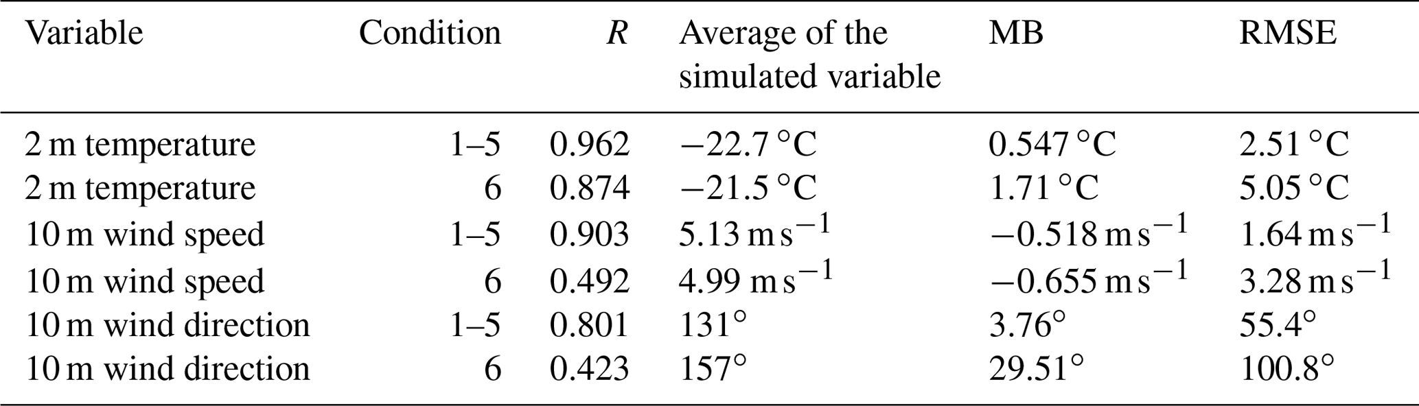

Figure 4Ozone at Utqiaġvik and at Summit from observations and simulations 1 (no halogens) and 3 (increased emissions, β=1.5). Modeled BrO mixing ratios are also shown. The data are shown at 06:00 GMT+0. The legend is the same for all panels.
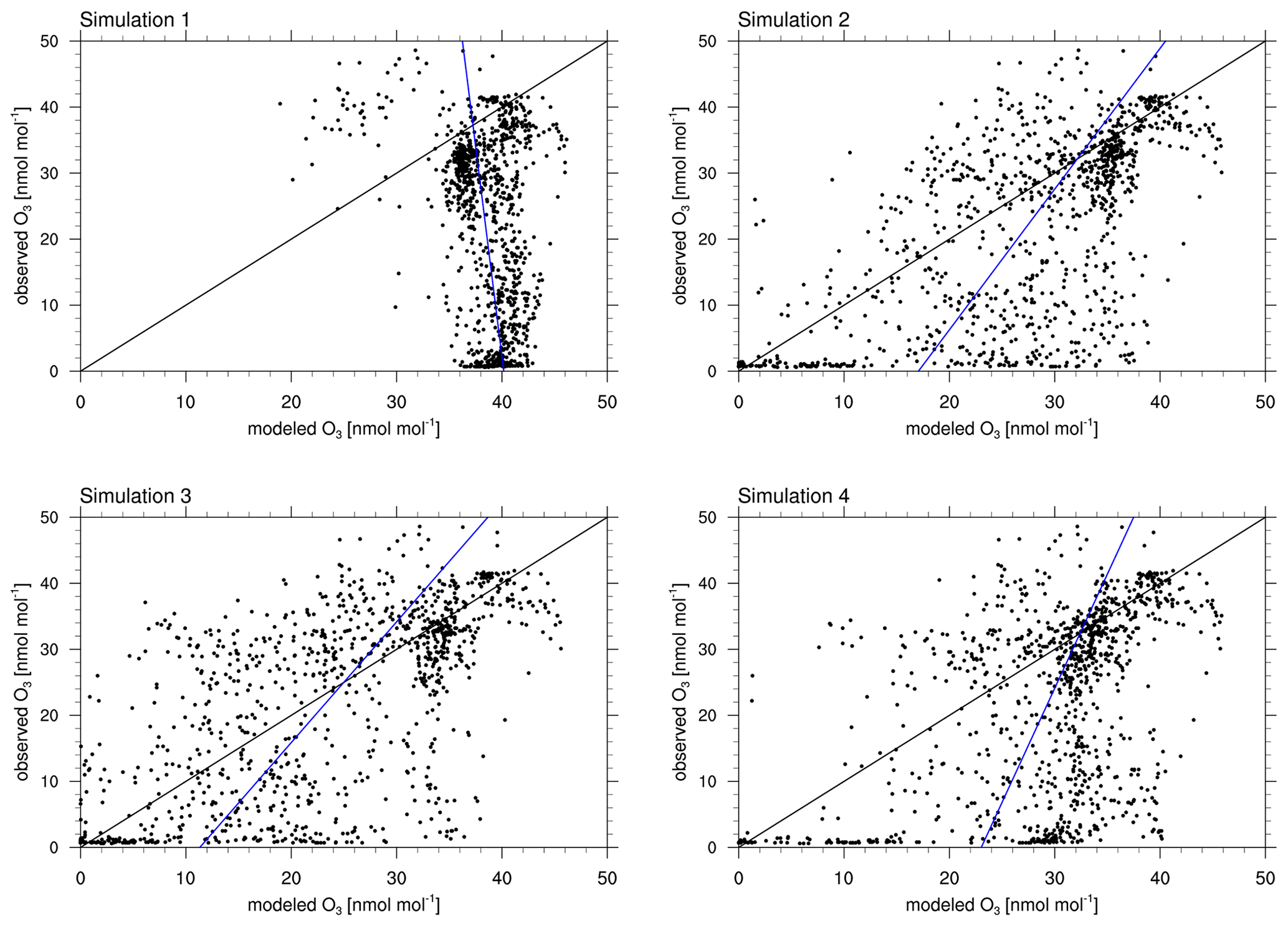
Figure 5Correlation of observed and modeled ozone at Utqiaġvik for the complete time range of 1 February through 1 May 2009. The black and blue lines show perfect agreement and the regression line of simulation and observation, respectively.
Table 4Statistics at Utqiaġvik and Summit for the ozone mixing ratio for 1 February through 1 May 2009.
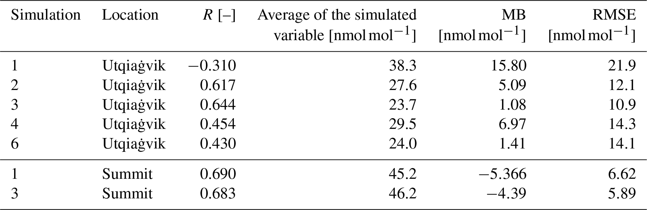
Figure 4 shows modeled and observed surface ozone and BrO at Utqiaġvik and at Summit. Only results of simulations 1 and 3 are shown for visual clarity. Figure S1 in the Supplement displays ozone mixing ratios modeled by simulations 1–4 and 6. The correlations of modeled and observed ozone can be seen in Fig. 5. Statistics are summarized in Table 4. Simulations 2–5 perform considerably better than simulation 1 for which halogen chemistry is turned off. Simulation 3 with enhanced emission performs best, with the correlation increasing from −0.31 to 0.644 compared to simulation 1. Quite a few ODEs are not captured by simulation 4, for which the emission probability for bromine emissions due to ozone under sunlight is reduced from 7.5 % to 0.1 %. Thus, direct emissions of bromine due to ozone are nearly completely turned off in simulation 4. This suggests a strong underestimation of bromine emissions without a direct emission of bromine due to ozone. A possible conclusion is that the bromine explosion mechanism is insufficient to explain ODEs in the Arctic, or the present bromine explosion scheme is incomplete, for instance with respect to emissions of bromide containing aerosols due to blowing snow and/or regions of increased β such as frost flowers. On 4 March an ODE is predicted by simulation 4 which, however, is not seen in the observations. The model predicts too large wind speeds for the preceding days, causing larger BrO emissions that ultimately result in a predicted ODE being advected to Utqiaġvik. For the first 3 weeks of February, the observations and results of simulations 2–6 are similar to those of simulation 1, in which halogen reactions are turned off, but afterwards, they differ increasingly. This suggests a weak initial influence of halogen chemistry during the first 3 weeks of February, which might be due to the low wind speeds during this time or due to the weak solar irradiation. Partial ODEs occur on 14, 17, 19, and 22 February 2009. The first full ODE in the observations occurred on 13 February, which is predicted by the model only as a partial ODE with 1 d of delay. The partial ODE observed on 17 February is found in simulations 2–5 with a delay of a few hours; simulations 3 and 4 find a stronger ozone depletion more consistent with the observations. On 21 February 2009, simulations 2 and 3 and simulations 4 and 5 predict partial and full ODEs, respectively, which are not seen in the observations. The strength of the ODEs in February is underestimated by the model. A possible cause for this is an overestimation of halogen deposition over land, which can be seen in the comparison to satellite data and is discussed in Sect. 3.3. Most of the model BrO capable of reaching Utqiaġvik can only be produced in the Bering Sea during February due to a lack of sunlight in the northern regions. Since BrO over land is removed too quickly in the model, BrO can only be sustained through heterogeneous reactions while being transported from Bering Sea to Utqiaġvik by trajectories that go mostly over the sea ice.
In March, both simulations and observations agree in the occurrence of at least partial ODEs during most of the month, whereas times without any ozone depletion at all are rare. Around 4 March, the model predicts a partial ODE in simulations 2–4, whereas simulation 6 predicts a full ODE, neither of which is found in the observations. Four days later, all simulations predict a partial ODE even though a full ODE is seen in the observations. The following ODE-free time period until 13 March is predicted in agreement with the observations; however, the full ODE on 15 March appears as partial ODE in all simulations, and the simulations with enhanced emission find the partial ODE to continue for 3 more days. The ODE on March 19 is found in simulations 2–6. The simulations predict a near-full recovery of ozone levels over 3 d, which, however, is interrupted in the observations on 21 March. The following ODE episodes are captured quite well by the simulations with an overprediction of ozone levels on 25 and 28 March. ODEs around 1, 14, and 18 April are underestimated in the simulations, whereas all other ODEs and ozone regeneration episodes are predicted quite well. At the end of April, the observations find enhanced ozone levels which are not captured by the model, not even by the simulation without the halogens. The enhanced ozone levels in the observations might be due to Arctic haze, i.e., enhanced photochemical ozone formation due to air pollution originating from lower latitudes. Walker et al. (2012) found that the decomposition of peroxyacyl nitrates (PAN), transported from lower latitudes or the upper troposphere to the Arctic boundary layer, can account for up to 93 % of the ozone production in the Arctic. The domain modeled in this work (see Fig. 1) does not consider the lower latitudes, so that the simulation itself cannot predict the production and transport of Arctic haze. However, pollution from the lower latitudes might be correctly modeled by the MOZART-4 model and thus be present in the lateral boundary conditions. The model does not find these enhanced ozone levels, which suggests inaccuracies in the MOZART-4 boundary conditions. Simulation 3 finds a partial ODE on 29 April, which is not present in the observations. The other simulations also find a slight decrease in the ozone mixing ratio; however, for these simulations, the BrO levels are not predicted to be large enough for an ODE to happen. Summarizing the entire period of 3 months, simulation 1 shows two ODEs where none were observed. Twenty-two ODEs are identified in the observations, half of which are found by simulation 2. Simulation 3, however, identifies four additional ODEs compared to simulation 2 which were not found in the observations. Simulation 3 misses only 6 of the 22 observed ODEs.
The results of simulation 6 differ strongly from the other simulation results starting mid March and the correlation coefficient R of 0.435 compared to simulation 2 with R=0.62. The RMSE is 14.1 compared to 12.1 nmol mol−1. The mean bias is improved, but this is simply due to the enhanced emissions, resulting in more ODEs, and not due to actually predicting the ODEs better. All statistics are worse compared to simulation 3. As discussed previously in this section, simulation 6 predicts meteorology much worse due to the lack of nudging, which also leads to wrong predictions in the ozone mixing ratio. As can be seen in the correlation plots, simulations 2 and 4 rarely find ODEs were there are none in the observations. There is a notable accumulation of points in all four simulations at ozone mixing ratios of about 30–40 nmol mol−1 for both the observations and the model. In this range of ozone mixing ratios, both the model and observations do not show any ODEs. Halogen chemistry, which has large uncertainties regarding the chemical reactions and the source of bromine, is less important in this case, which explains the high density of points in this regime. This accumulation is denser for simulations with weaker bromine emissions, since those simulations less often predict ODEs which do not exist in the observations. There is an additional accumulation of points around an ozone mixing ratio of 0 in both the model and the observations for simulations 2–4, which are ODEs found by both model and simulation. This accumulation is less dense for simulation 4 compared to simulations 2 and 3. Simulation 4 performed worst regarding both mean bias and RMSE. In simulation 4, there is an accumulation of points at around modeled ozone values of 30 nmol mol−1 and observed ozone values of 0, which are the ODEs missed by the simulation, which suggests an underestimation of the occurrences of ODEs. Simulation 4 with a strongly enhanced β=2.0 but a reduced bromine emission due to direct bromide oxidation by ozone during the daytime (Φ=0.1) suggests that the bromine explosion mechanism alone is insufficient to properly predict the bromine production.
Simulations 2–4 and 6 reproduce ozone levels and ODEs much better than simulation 1, where the mean bias is smaller by at least 9 nmol mol−1. For simulation 3, all statistics are improved compared to the base simulation 2, with both the correlation and RMSE being only slightly better and the mean bias being about 80 % smaller (1.1 vs. 5.1 nmol mol−1) than in simulation 2. Figure 5 shows a strong increase in the number of ODEs that occur in the model but not in the observations, which explains the strongly improved mean bias while the other statistics only improved slightly.
At Summit, ODEs were found by none of the simulations and not in the observations which lack data for 29 April as can be seen in Fig. 4. The differences between a simulation without halogens and with halogens are negligible. Ozone mixing ratios are underpredicted with a mean bias of −4.3 nmol mol−1 for simulation 2. This is in contrast to Utqiaġvik, where ozone was generally overpredicted. In April, ozone levels at Summit are found to exceed 60 nmol mol−1 for several time periods in the observations. This is probably due to the high elevation of 3200 m a.s.l. of Summit in contrast to Utqiaġvik. At Summit, the time with the highest ozone level, which occurs on 18 April, is found by the model. The high ozone mixing ratio in the model is due to stratospheric ozone, reaching the troposphere due to a tropopause fold event as shown in Fig. 6. The other time periods of enhanced ozone levels found by the observations may also be due to a tropopause fold or possibly Arctic haze events.
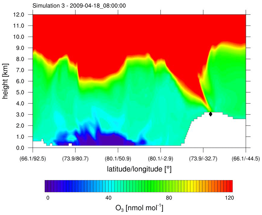
Figure 6Ozone mixing ratio obtained from simulation 3 (β=1.5) against height along a horizontal line through Summit; see Fig. 1. A tropopause fold reaches Summit (⧫). The time zone is GMT+0.
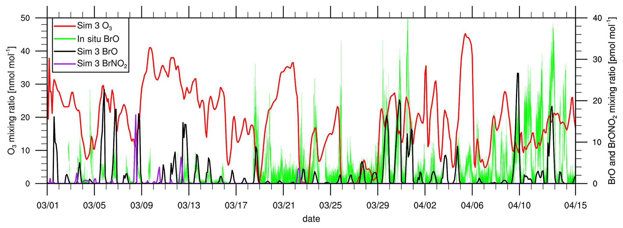
Figure 7Comparison of modeled BrO and in situ observations of BrO at Utqiaġvik (Liao et al., 2011) and modeled O3 and BrNO2; the numerical results are for simulation 3. The data are shown at 00:00 GMT+0.
Figure 7 shows modeled BrNO2 and BrO of simulation 3 and in situ observations of BrO (Liao et al., 2012) at Utqiaġvik. In order to improve the comparability of the observed data with a 10 min resolution and the model results, which were saved every 2 h, a seven-point moving average is applied to the observations, taking the average of the time point under consideration and three time points prior to and after that time point. Modeled BrO is underpredicted with a mean bias of −1.65 pmol mol−1, and a correlation of 0.472 is found. In early to mid March, BrO is less underpredicted with an overprediction of BrO for some days. For most of these days, enhanced BrO levels are due to NOx-catalyzed release of reactive bromine. NOx is emitted at Prudhoe Bay and can then produce N2O5, which further releases BrNO2 on FY ice via the heterogeneous reaction
BrNO2 can then photolyze to Br, which may further release bromine on FY ice through the bromine explosion mechanism. In the current model, the above heterogeneous reaction is the only source of BrNO2, so that any enhanced mixing ratios of BrNO2 at Utqiaġvik can be attributed to polluted air from Prudhoe Bay producing bromine on FY ice through the heterogeneous reaction with N2O5. As can be seen, for many of the days in early March, there are enhanced BrNO2 mixing ratios preceding large BrO levels. Enhanced modeled BrO on 14, 17, and 20 February (see Fig. 4) is coincident with large BrNO2 mixing ratios caused by polluted air from Prudhoe Bay, which is transported over sea ice. A similar phenomenon was found by Simpson et al. (2018), who discovered large BrO concentrations in February 2017, which are attributed to nighttime photolabile bromine production, possibly by N2O5, over sea ice. These photolabile species may be transported to lower latitudes where they might be photolyzed. A further discussion of modeled N2O5 can be found in Sect. S6 in the Supplement. Custard et al. (2015) studied the role of NOx in bromine chemistry from 24 March 2009 to 3 April 2009 at Utqiaġvik using a box model. They found a suppression of ozone destruction for a high-NOx case (concentrations in the range of 800 to 1600 pmol mol−1). During this time frame, the simulation with WRF-Chem predicts negligible production of reactive bromine due to N2O5. In Fig. S6 in the Supplement, modeled NOx, BrONO2, HOBr, and BrO are shown for the time range considered by Custard et al. (2015). Modeled NOx is elevated from 24 to 26 March and again on 2 April, similar to the measurements of NOx shown in Fig. 2 of the paper of Custard et al. (2015). However, the present model does not find NOx mixing ratios on the order of 10 000 pmol mol−1 as identified on 24–27 March in the measurements. The typical modeled NOx concentrations are in the range of 50 to 1000 pmol mol−1, i.e., between the high- and low-NOx scenarios of Custard et al. (2015). The predicted values of BrONO2 shown in Fig. S5 in the Supplement of this paper compare quite well with those of Custard et al. (2015) (see Fig. 7c of that work), with peak values around 50 pmol mol−1. From the end of March to 15 April, however, the mixing ratio of modeled BrO is smaller, whereas the BrNO2 mixing ratio drops to almost 0. Due to the higher temperature and stronger sunlight, N2O5 becomes less stable and its mixing ratio drops, suppressing bromine production due to N2O5. At the same time, observed BrO mixing ratios strongly increase. The underprediction of modeled BrO for these later dates is likely due to a general underprediction of bromine near coastal regions and on land, which will be further discussed in the following sections.
3.2 Vertical ozone and temperature profile at Utqiaġvik
Ozone sonde sounding data (Oltmans et al., 2012) produced near Utqiaġvik are used to validate vertical ozone profiles. Measured ozone and potential temperature for the upward flight of the sonde in the first 2 km are shown in Figs. 8 and 9 together with the simulation result of the column of the nearest grid cell. The simulation result is interpolated linearly in time to the starting time of the sonde flight.
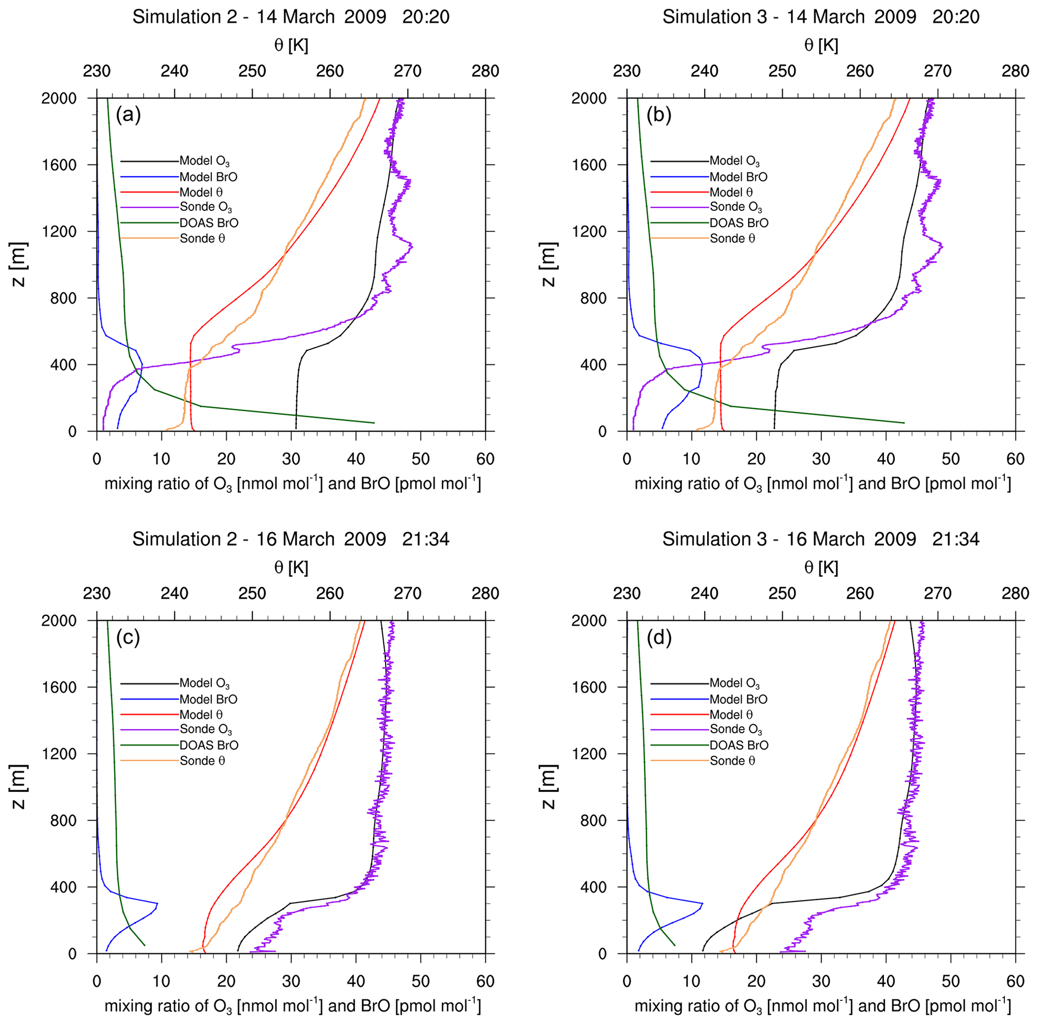
Figure 8Vertical profiles of measured and modeled ozone, of potential temperature θ, and of BrO at Utqiaġvik on 14 March (a, b) and on 16 March (c, d) 2009. The time zone is GMT+0. Measurements are from upward flights using ozone sondes (Oltmans et al., 2012) and DOAS measurements (Frieß et al., 2011).
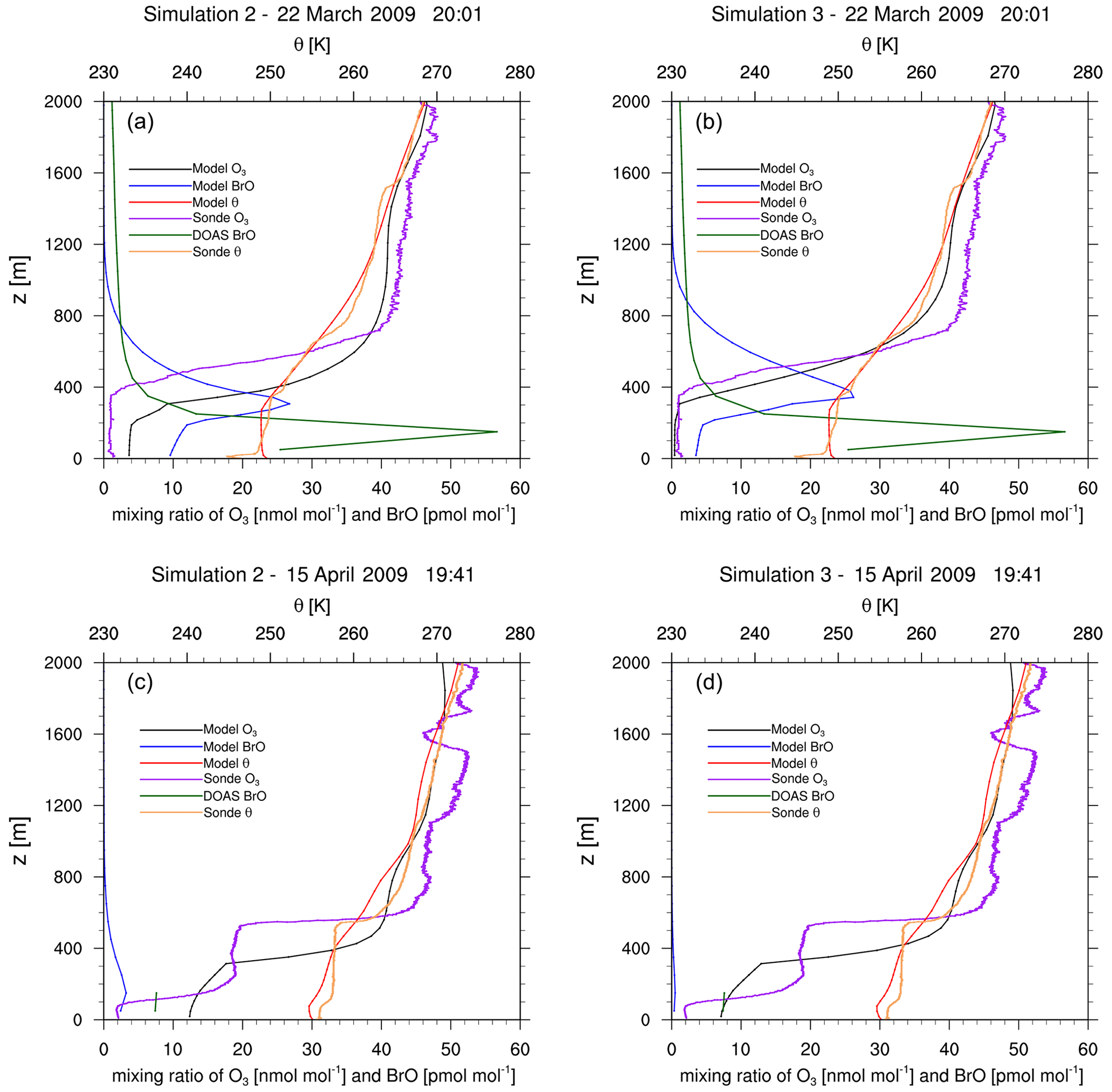
Figure 9Vertical profiles of measured and modeled ozone (simulation 2 (a, c) and simulation 3 (b, d), respectively), of potential temperature θ, and of BrO at Utqiaġvik on 22 March (a, b) and 15 April (b, d) 2009. The time zone is GMT+0. Measurements are from upward flights using ozone sondes (Oltmans et al., 2012) and DOAS measurements (Frieß et al., 2011). On 15 April, only the observed BrO mixing ratio in the lowest 100 m is accurate due to very poor visibility.
Figures 8 and 9 show vertical profiles at Utqiaġvik for various dates. For 14 March, the model fails to find the shallow surface inversion (boundary layer height smaller than 50 m) possibly due to a lack of vertical resolution. The boundary layer height of about 350 m in the observation is overpredicted by approximately 200 m by the model, which might also partially explain the finding of a partial ODE by the model instead of a full ODE as seen in the observations. For this day, simulation 3 performs slightly better than simulation 2. Two days later, both the observations and the simulations show partial ODEs. Simulation 2 predicts the ozone profile very well. The temperature profiles are quite different; however, both model and observations show an inversion at a similar, low height. For 22 March, the enhanced emission case correctly predicts a full ODE, capturing both ozone and temperature profile quite well. The model is however unable to capture a surface inversion. On 15 April, a surface inversion with a second inversion at approximately 500 m is found in the observations. The MYJ PBL scheme also predicts a surface inversion; however it fails to predict the second inversion properly, as can be seen by the lack of a second ozone plateau. While the model is unable to capture the complex boundary layers perfectly, the ozone profiles shows many similarities to the observed profile. For a better prediction, more grid levels closer to the surface and improvements to the PBL schemes might be needed. Even that, however, might not be sufficient, since PBLs in the Arctic can be influenced by very small-scale structures such as open leads, which were found to play an important role in the ozone recovery after an ODE due to down-mixing of ozone-rich air from the free troposphere (Moore et al., 2014) and which would require high-resolution sea ice data. Additionally, an accurate modeling of surface inversions might require very high vertical resolutions, which are difficult to obtain in a synoptic-scale simulation.
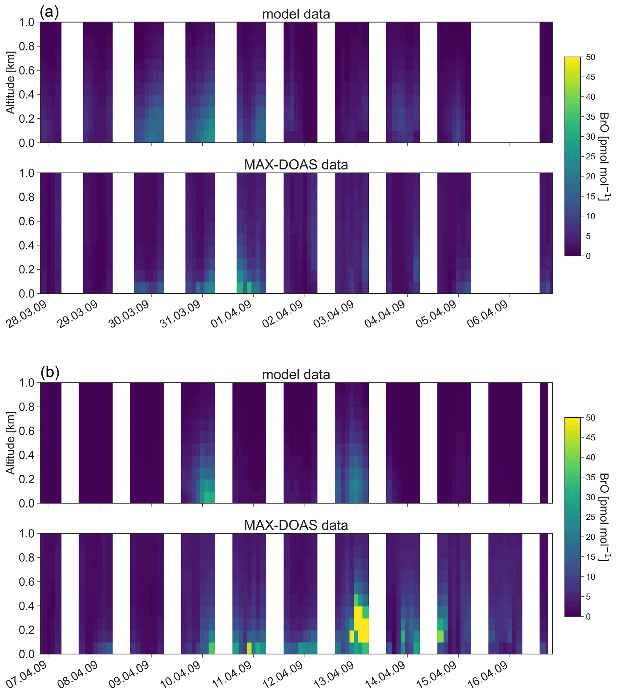
Figure 10Vertical profiles of BrO from 28 March to 16 April 16 2009 at Utqiaġvik. The data are shown at 00:00 GMT−9 (LT at Utqiaġvik). (a) Modeled BrO convoluted with the MAX-DOAS averaging kernel; (b) BrO observed with MAX-DOAS.
Figure 10 shows modeled vertical BrO profiles convoluted with the MAX-DOAS averaging kernel from 28 March 2009 to 16 April 2009 at Utqiaġvik in comparison to BrO measured with a MAX-DOAS instrument (Frieß et al., 2011). The time range from 26 February 2009 to 27 March is illustrated in Sect. S5, Fig. S4, in the Supplement. BrO from the same observation dataset is shown in Figs. 8 and 9. On days with good visibility, the observed data are sensitive for the first 1–2 km. As can be seen, model and observations agree on most dates on the presence of BrO. However, modeled BrO tends to be elevated in comparison to the observations, which can be seen for all days shown in Figs. 8 and 9 and on 31 March and on 1 and 10 April in Fig. 10. This is likely due to an underestimation of bromine emissions over snow-covered land, which is also discussed in the next section. Since the model assumptions only allow for partial recycling of bromine over land but not for new emissions, in the lowest grid cells, bromine is lost due to depositions, which results in the elevated modeled BrO profiles. On 9 and 13 March, the model overpredicts BrO. The high BrO mixing ratio on those two dates is due to a heterogeneous reaction involving N2O5; see Fig. 7. Frieß et al. (2011) found correlations of the aerosol extinction and BrO, which led to the hypothesis that BrO is released in situ during snowstorms. Currently, there is no model with blowing snow included, which may explain the underprediction of modeled BrO at some days.
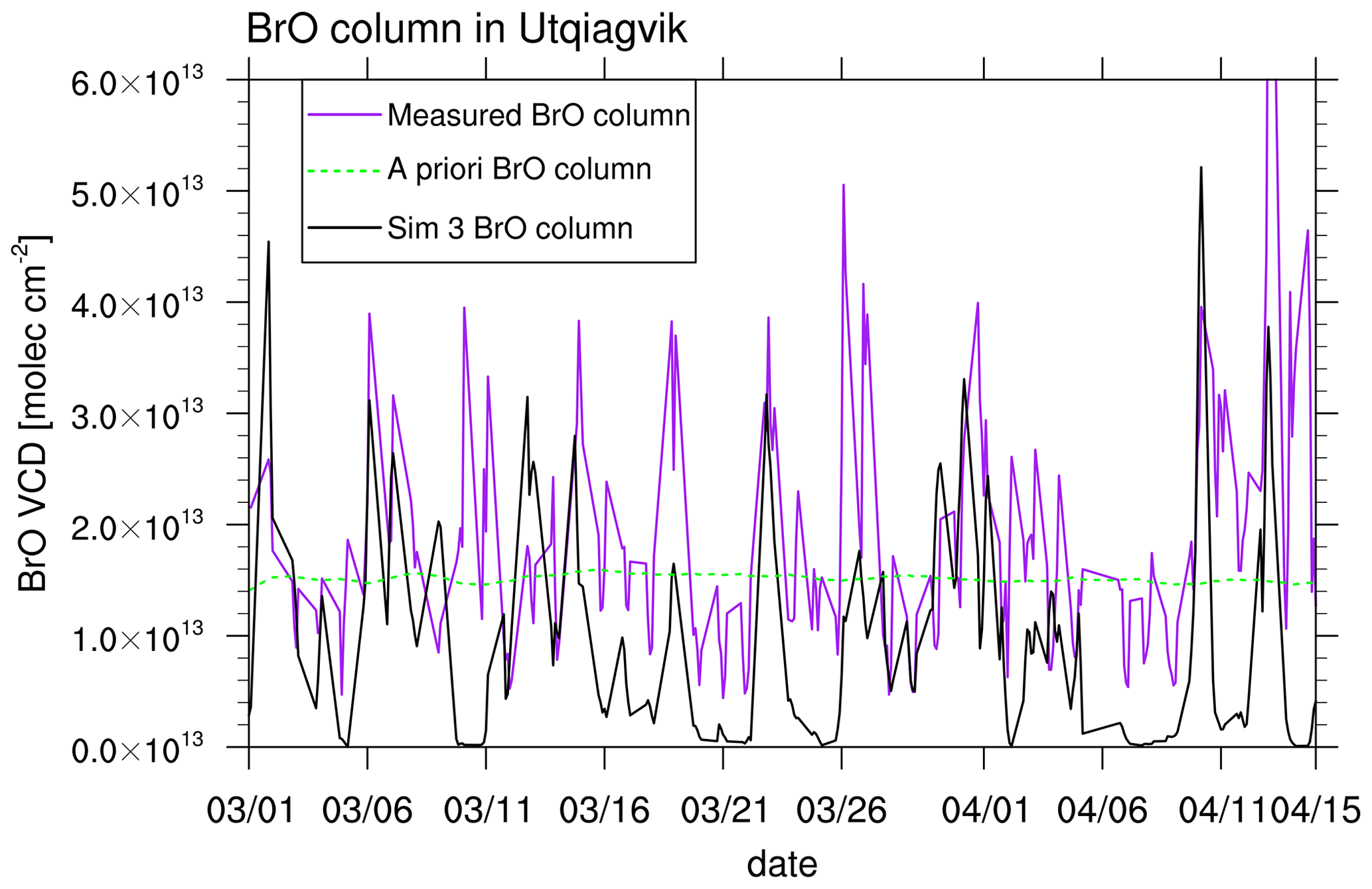
Figure 11Comparison of modeled (simulation 3) BrO VCDs and measured BrO VCDs from MAX-DOAS at Utqiaġvik (Frieß et al., 2011). The data are shown at 00:00 GMT−9 (LT at Utqiaġvik). Also shown is an a priori BrO column for days with low visibility.
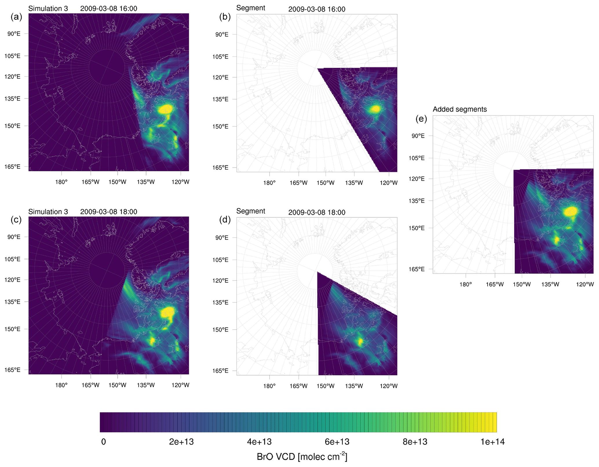
Figure 12Illustration of the averaging of modeled BrO VCDs. Shown is 8 March 2009, 16:00 and 18:00 UTC. (a, c) Full instantaneous BrO VCDs. (b, d) Corresponding 60∘ segment. (e) Added segments.
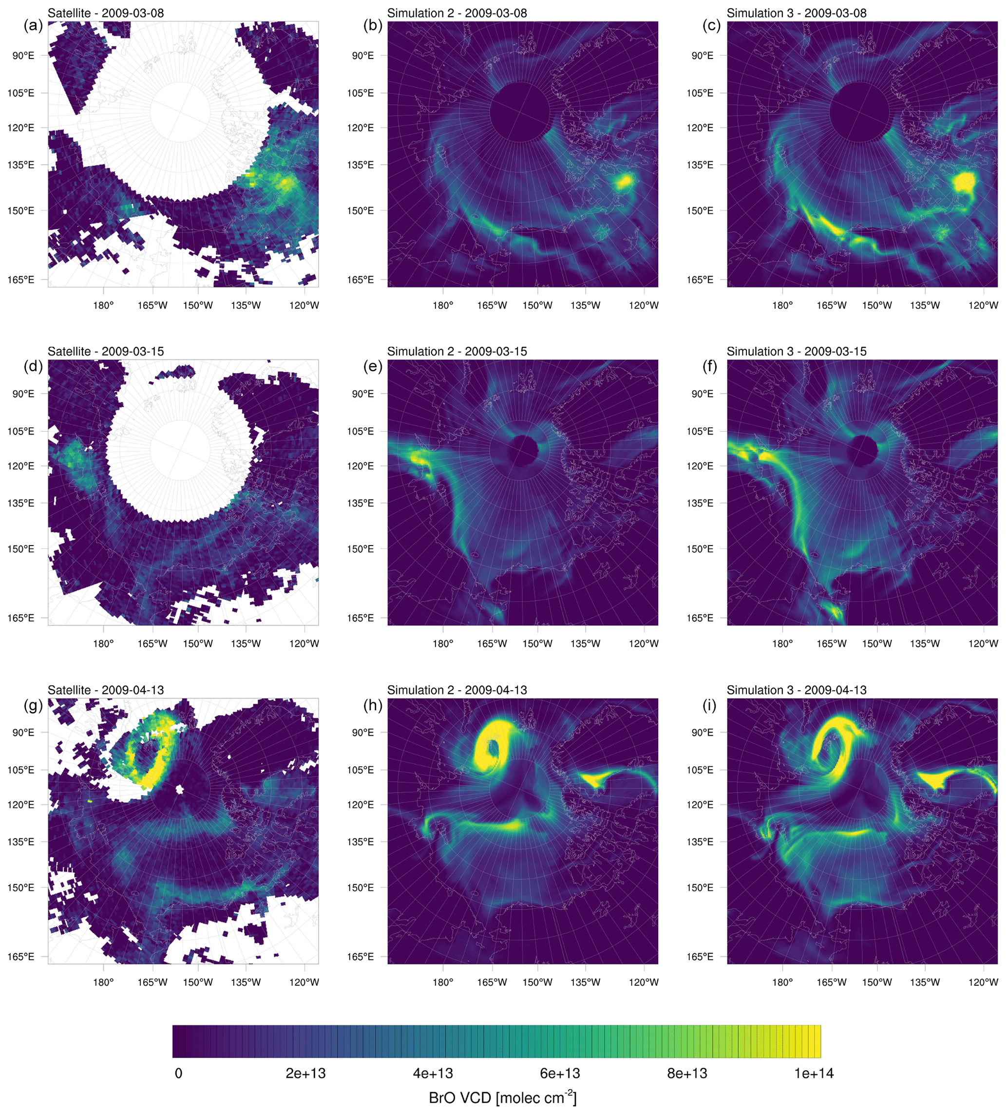
Figure 13BrO VCDs on selected days in the year 2009. (a, d, g) Satellite measurements. (b, e, h) Simulation 2 (β=1.0). (c, f, i) Simulation 3 (β=1.5).
Figure 11 shows vertically integrated modeled (simulation 3) and measured BrO (Frieß et al., 2011) over the first 2 km. As can be seen, the BrO column is generally underpredicted by the model with a mean bias of . This may partly be attributable to the underprediction of BrO over land in the model; however, there seems to be an offset of around 5.0×10¹² in the measurements. A correlation of 0.427 is found.
3.3 Tropospheric BrO VCDs
GOME-2 satellite tropospheric BrO VCDs (Sihler et al., 2012) described in Sect. 2.6.1 are compared with BrO VCDs evaluated from the numerical simulations. All satellite BrO orbits of the same day are averaged and plotted in one figure, where missing satellite data are neglected. Since stratospheric BrO is not generated in the present model, all BrO predicted by the model is of tropospheric origin. Thus, model BrO VCDs are calculated by integrating BrO concentrations vertically from the bottom to the top of the calculation domain. Simulation results are stored every 2 h starting at 00:00 UTC. Each output is assigned a 60∘ segment of a circle with its origin at the North Pole. The segment is centered on a longitude, conforming to GOME-2 orbits for that time. The BrO VCDs are averaged with their neighboring segments with a weight of unity at the center of the segment, and decreasing linearly to 0 at the edge of the segment. This procedure is a linear time interpolation and smoothes the resulting model BrO VCDs. Figure 12 displays the simulated instantaneous BrO VCDs on 8 March 2009, 16:00 and 18:00 UTC. On the left there are 2 of the 12 full BrO VCDs saved for each day and in the middle the corresponding 60∘ segment multiplied by a weight of unity at the center, which linearly decreases to 0 at the edges of the segment. On the right, the added segments are shown. This procedure is done each day for all 12 time points. Thus 12 segments, not just the two segments shown in Fig. 12, are added for the average of 1 d, covering the whole domain.
Figure 13 shows daily averages for the satellite data and simulations 2 and 3 on selected days. On 8 March, both the model simulation and the observations show a high BrO VCD in Nunavut, including King William Island. However, the models predict BrO VCDs to be strongly concentrated in a small area, whereas the satellite BrO cloud is spread out more and reaches deeper into the Canadian mainland. On 15 March, both model simulations and satellite observations find a bromine cloud over the Laptev Sea, reaching to the Siberian land mass. The modeled BrO VCDs are more pronounced, with simulation 3 having a different distribution of BrO being less consistent with the observations than simulation 2. The enhanced emissions in simulation 3 cause a stronger ODE in that region, which in turn depletes BrO in the ozone-depleted area. Ozone mixes back into the ozone-depleted area from the edges of an ODE, which allows BrO to form there which is the reason for the elevated BrO levels seen at the edges of the ODE. The bromine cloud is predicted by the model to extend to the Chukchi Sea in a thin stripe, which is barely seen in the observation. In both model results, a small BrO cloud in Hudson Bay is found, which is more pronounced and less consistent with the observations for simulation 3. On 13 April, a ring-like BrO structure can be seen north of the Kara Sea. The BrO-free center of the ring is due to ozone depletion. Both simulations correctly find a BrO-free area near the North Pole. An enlarged ODE is predicted, resulting in a thinner ring more consistent with the observations. The model, however, underpredicts BrO clouds near the Alaskan coast and finds enhanced BrO VCDs in Greenland in contrast to the observations.
In summary, both simulations 2 and 3 appear to be successful in capturing the general structures. Some of the differences might be explained by a higher model resolution (20 km×20 km) compared to the satellite data with a resolution of 40 km×30 km, resulting in more detailed structures in the model. Other differences might be explained by the already discussed errors in the meteorology and underprediction of BrO over land discussed below.
The uncertainties in the satellite data contribute to the differences between model and observations. According to Sihler et al. (2012), they are typically below 50 %. Accordingly, differences in absolute values between model and satellite measurement might to a substantial part be caused by measurement uncertainties. However, the spatial patterns found in the satellite data are hardly affected because measurements which are strongly influenced by clouds (cloud shielding) are filtered out using the sensitivity filter of 0.5 for the air mass factor of the lowest 500 m (Sihler et al., 2012).

Figure 14BrO VCDs in the year 2009 averaged over 1 month. (a, d, g) Satellite measurements. (b, e, h) Simulation 2 (β=1.0). (c, f, i) Simulation 3 (β=1.5).
Figure 14 shows monthly averages for the satellite data and results of simulations 2 and 3. Pratt et al. (2013) and Peterson et al. (2018) reported BrO observations using MAX-DOAS over the tundra snowpack, which show elevated BrO levels up to more than 100 km inland. Peterson et al. (2018) found higher BrO concentrations over the tundra than over FY ice. In contrast to that, the simulations conducted in this work underpredict BrO over land and near coasts, which is most likely due to the assumptions in the emission scheme. In the model, it is assumed that snow surfaces have no salt content, which makes depositions of bromine species (excess HOBr is lost) over land a sink, as opposed to depositions over MY ice, which are neutral (excess HOBr is released as BrCl), and over FY (HOBr always releases Br2), which are a source of bromine in most cases. With a deposition velocity of 1 cm s−1 and a boundary layer height of 200 m, bromine is removed at a timescale of approximately 5 h over land by surface depositions and possibly even faster by depositions to aerosols. The assumption of zero bromide content of snow covering land or MY ice is of course an idealization and not always correct in reality (Simpson et al., 2005; Jacobi et al., 2012; Krnavek et al., 2012; Peterson et al., 2018, 2019), contributing to the underprediction of BrO over land mentioned in this paragraph. Future simulations should aim to find ways to incorporate the salinity, pH, and the ratio of the snowpack, which where found to be important parameters for the production of Br2 (Pratt et al., 2013; Wren et al., 2013; Peterson et al., 2019). BrO VCDs are also underpredicted near the boundaries, which is due to the value of 0 of halogens at the boundary. The model overpredicts BrO VCDs at Baffin Bay and at most locations featuring FY sea ice with the exception of the Bering Sea, probably due to its proximity to a domain boundary. The overprediction over FY sea ice is not surprising with the assumption of unlimited BrO in FY sea ice. A relaxation of this assumption, e.g., by allowing finite salt content could solve the issues both over snow covering FY ice, by limiting the bromine emissions, and over land, by allowing salt content of more than 0 and storage instead of loss of deposited bromine. The model prediction for BrO in February is generally too small, which is probably due to a lack of sunlight at higher latitudes and the underprediction of BrO over land. It should be noted that the satellite data are quite incomplete during February and biased towards the end of February, also due to a lack of sunlight necessary for satellite measurements in early February, whereas the model VCDs weights all of February equally.
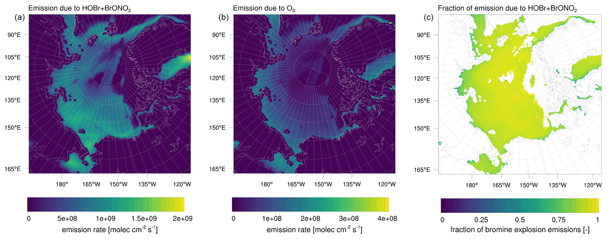
Figure 15Emission rate of Br2 (a) due to HOBr+BrONO2 and (b) due to bromide oxidation by ozone from the snow surface for simulation 3, averaged over the complete simulation period. Ratio of Br2 emissions (c) due to HOBr and BrONO2 to total Br2 emissions on FY ice.
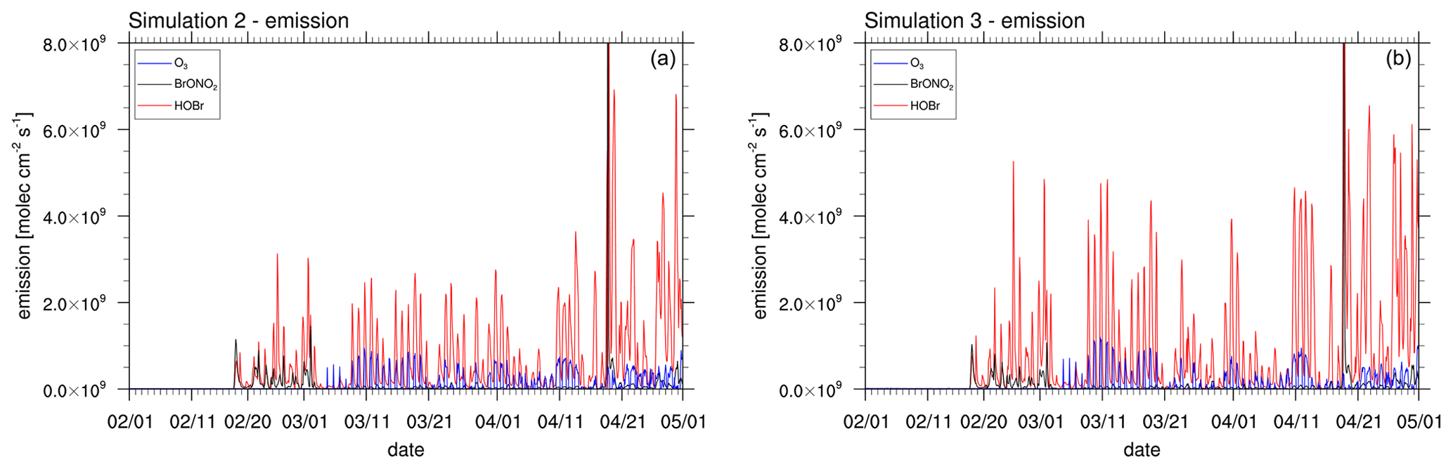
Figure 16Emission rate of Br2 due to HOBr and BrONO2 and due to bromide oxidation by ozone from the snow surface at coordinates 78∘ N, 178∘ W for (a) simulation 2 with β=1 and (b) simulation 3 with β=1.5. The data are shown at 06:00 GMT+0.
The emission rate of Br2 due to HOBr+BrONO2 and due to bromide oxidation by ozone from the snow surface averaged over the entire simulation period is shown in Fig. 15 for simulation 3. In Fig. 16, the production of Br2 from the snow is shown at coordinates 78∘ N, 178∘ W plotted against time. The location has been chosen because it is over FY sea ice and is a strong production site for the bromine that may affect ODEs at Utqiaġvik. As can be seen in these figures, most of the bromine is produced by HOBr, i.e., the bromine explosion mechanism, whereas the oxidation of bromide by ozone provides an initial seed of the bromine formation which then is enhanced by bromine explosion where BrONO2 plays a smaller role than HOBr. Due to a lack of sunlight, bromine is produced only during the second half of February by the bromine explosion and after 1 March 2009 by the bromide oxidation due to ozone.
In the present parameterization, the latter strictly requires an SZA of less than 85∘ for a fast release, whereas the bromine explosion mechanism has a more continuous dependence on SZA. The Br2 photolysis needed by both emission mechanisms requires relatively longwave light and may thus occur even at SZAs slightly above 90∘. The bromine explosion additionally requires HO2 in order to produce HOBr. HO2 is mostly formed by a photolysis of various organic species with shortwave UV and thus occurs generally at smaller SZA; however, it can also be supplied by reactions involving organic compounds, NOx, and/or OH or by their transportation from lower latitudes. Thus, in the present parameterization, the bromine explosion may occur locally at higher SZAs than the bromide oxidation due to ozone.
Emission rates of Br2 from other studies are as follows. In February 2014, Custard et al. (2017) measured Br2 fluxes of 0.07–1.2×10⁹ above the snow surface near Utqiaġvik with a maximum around noon. Wang and Pratt (2017) found snowpack Br2 emissions of 2.1×10⁸ on 15 March 2012 and 3.5×10⁶ on 24 March 2012 in a modeling study. Emission fluxes due to the bromine explosion (HOBr+BrONO2) are typically between 2–3×10⁹ (simulation 2) or 4–5×10⁹ (simulation 3) around noon and thus are at the higher end of the mentioned values. Bromide oxidation due to ozone, which plays the role of direct snowpack emissions in the present model, is rarely larger than 1×10⁹ with an average of around 2×10⁸ near Utqiaġvik, which compares quite well to the range found by Custard et al. (2017) while being larger than the values calculated by Wang and Pratt (2017).
For a simulation of 3 months, it should be expected that errors in the simulation pile up, especially considering the nonlinear stochastic nature of ODEs. The meteorological state should be consistent due to the data assimilation via nudging; however, the errors in the chemistry model could grow large over time. As an example, wrongly predicting an ODE probably causes a delay of an ODE at a later date due to the lack of O3, reducing bromine emissions. A test for this is performing a new start of a simulation at a later date, where no ODEs occurred and in which the atmosphere is clean of bromine. For this purpose, simulation 5 was conducted, which is identical to simulation 3 except that the simulation starts on 16 March using ERA-Interim and MOZART-4 data as well as a near-zero bromine concentration, as described in Sect. 2.5. These new simulation results are then compared to simulation 3 which started in February.
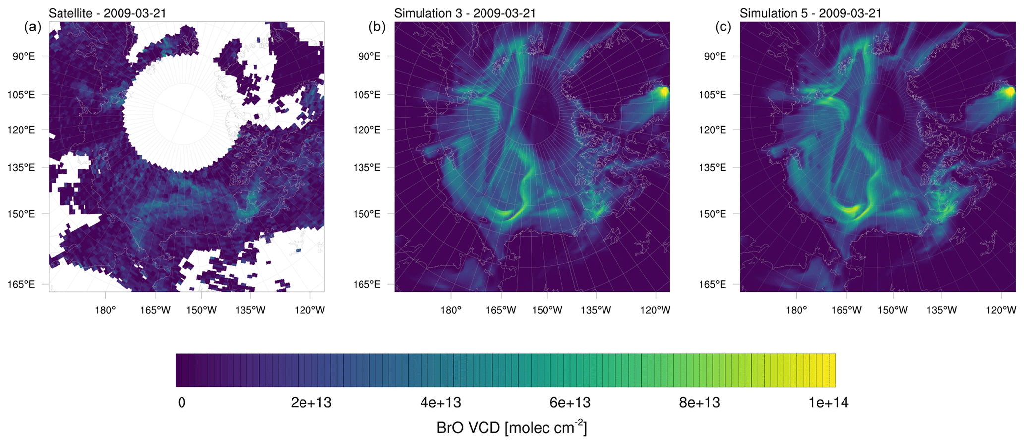
Figure 17(a) BrO VCDs on 21 March 2009 from observations and simulations initiated on (b) 1 February (simulation 3) and (c) 16 March (simulation 5). The simulations differ only in the start time.
It is found that these two simulations become very similar after approximately 5 d; see Fig. 17 which shows the BrO VCDs. After approximately 8 d, the BrO VCDs become nearly indistinguishable. Average BrO concentrations in April are not shown here but are also nearly identical for both simulations. Reasons for the two simulations with different starting times to show such similar results after a few days is due to a combination of several factors. While there is no chemical nudging, the chemical boundary conditions strongly affect the simulation and act similarly to chemical nudging. Assuming a constant wind speed of 20 km h−1 (corresponding to approximately 5.5 m s−1), a chemical species can be transported from a 2000 km distant boundary to the center of the domain on a timescale of as low as 4 d. Due to the meteorological nudging, chemical boundary conditions are transported in the same way in both simulations. Chemistry boundary conditions transported over land or in the free troposphere behave similarly in simulations 3 and 6, since several aspects of chemistry over land and in the free troposphere are nearly unaffected by the addition of halogen chemistry. Thus, chemical species coming from the lateral boundary condition will only be affected by the halogen chemistry once they reach the sea ice or are mixed into the boundary layer from aloft.
The emission of bromine due to bromide oxidation by O3 is independent of reactive bromine mixing ratios and not of autocatalytic nature as in the bromine explosion mechanism. While it is only responsible for a small fraction of emitted bromine, it produces the initial bromine needed for a bromine explosion. The present emission scheme can be very fast, producing full ODEs in less than a day. All of these effects allow ozone coming from the lateral boundary condition to be depleted in a similar way in simulations 3 and 6 even with leftover bromine from a previous ODE.
Three-dimensional unsteady simulations of ozone depletion events in the Arctic from 1 February 2009 through 1 May 2009 have been performed using WRF-Chem. Simulations with different parameter settings are compared to observations from different sources at Utqiaġvik, Alaska and Summit, Greenland. A simulation using standard MOZART–MOSAIC chemistry without halogen chemistry resulted in an unrealistic ozone mixing ratio at Utqiaġvik, anti-correlating with observations and a strong bias for large ozone mixing ratios, which demonstrates the impact of halogen chemistry on the prediction of ODEs.
Bromine may be emitted by the extended bromine explosion mechanism and/or oxidation of bromide by ozone directly from the snow covering sea ice. The reactive surface ratio β accounts for non-flat surfaces such as snow or ice and controls the emission strength. Both simulations with a standard emission (simulation 2, β=1.0) and a simulation with enhanced emission (simulation 3, β=1.5) perform with correlations to observations of more than 0.6 at Utqiaġvik for both vertical ozone profiles and BrO VCDs. Enhancing the emission strongly improves the mean bias, whereas correlation and RMSE only improved slightly with enhanced emissions, which is likely due to an overestimation of BrO emissions which occur more frequently. Generally, ozone depletion at Utqiaġvik is somewhat underpredicted by both simulations. ODEs identified by the model that are not present in the observations are rare: simulations 2 and 3 identify two and six ODEs, respectively. Simulation 2 finds half of the 22 observed ODEs, whereas simulation 3 improves this prediction to more than two-thirds of the observed ODEs. Iodine chemistry was neglected in this study, which may contribute to the underprediction of ODEs at Utqiaġvik.
At Summit, the observations and simulations agree in identifying no ODEs. A tropopause fold is found by the simulations at the end of April 2009 in agreement with the observations.
At Utqiaġvik, temperature is slightly overpredicted and wind speed slightly underpredicted, both of which may contribute to an underprediction of ODEs. BrO VCDs are found to be consistent with satellite observations. However, an underprediction of BrO VCDs over land and an overprediction of BrO VCDs over FY ice is apparent. A good qualitative agreement of modeled BrO with in situ and MAX-DOAS measurements at Utqiaġvik was found; however the underprediction of BrO over land was also apparent. This is probably due the assumptions of the emission scheme in the model: snow covering FY ice is assumed to have unlimited bromide content, resulting in an overestimation of BrO emissions, whereas snow over land has no halogen content, overestimating the removal of BrO. More realistic assumptions in a future study, such as an inclusion of snowpack emissions over land or a blowing snow parameterization, may improve the results. Emissions of bromine due to N2O5 were found to be important in February to mid March but were of little relevance in the later months, since N2O5 becomes less stable with growing temperatures and sunlight intensity.
The direct emission of bromine due to bromide oxidation by ozone is found to be very important throughout the entire simulation, since it provides an initial seed of bromine which then triggers the bromine explosion. Simulation 4 with deactivated bromide oxidation by ozone under sunlight strongly reduces Br2 emissions even though the value of β has been set to 2.0. Therefore, simulation 4 is inferior to simulations 2 and 3 with a reduced overall prediction skill of ODEs. With an even larger emission rate, the bromine explosion mechanism alone does not produce enough BrO to explain the observations, which is likely due to a missing trigger of ODEs to provide the bromide oxidation by ozone. An alternative trigger of ODEs that may be worthwhile studying in future is the bromide oxidation by the hydroxyl radical.
Meteorological nudging is found to be very important. A simulation with enhanced emissions by 50 % but disabled meteorological nudging (simulation 6) performs much worse compared to simulations 2 and 3. At Utqiaġvik, the prediction of meteorological variables such as temperature, for which the mean bias increased by a factor of 3 and the RMSE by a factor of 2, becomes worse during the simulation; in particular, the second half of the simulation has a strong bias towards larger temperatures and a poorer skill for predicting ozone. Simulations 2 and 3 with β equal to 1.0 and 1.5, respectively, are found to perform best, where simulation 3 is somewhat superior to simulation 2 at the cost of an overprediction of BrO at some times. It might be worthwhile searching for an optimal setting for β in a future study.
In a follow-up study it is planned to simulate ODEs in the year 2019, for which the new TROPOMI (TROPOspheric Monitoring Instrument) BrO VCDs with a high resolution of 5.5 km×3.5 km are available. For this purpose, the grid resolution will be increased in order to allow for a comparison of the more refined observation data.
The software code and data may be obtained from the corresponding author upon request. The GOME-2 level 1 data for BrO, O3, and NO2 are available at https://doi.org/10.15770/EUM_SAF_O3M_0011 for BrO (AC SAF, 2017a), https://doi.org/10.15770/EUM_SAF_O3M_0009 for O3 (AC SAF, 2017b), and https://doi.org/10.15770/EUM_SAF_O3M_0010 for NO2 (AC SAF, 2017c). ERA-Interim data were provided courtesy of ECMWF (https://apps.ecmwf.int/datasets/data/interim-full-daily/levtype=pl/, Dee et al., 2011). In situ data for ozone at Utqiaġvik (https://gml.noaa.gov/aftp/data/ozwv/SurfaceOzone/BRW/1973-2010/BRW_Ozone_hourly_2009, McClure-Begley et al., 2014) and Summit (https://gml.noaa.gov/aftp/data/ozwv/SurfaceOzone/SUM/2000-2010/sum_ozone_hourly_2009.dat, McClure-Begley et al., 2014) as well as meteorology at Utqiaġvik (https://gml.noaa.gov/aftp/data/meteorology/in-situ/brw/met_brw_insitu_1_obop_hour_2009.txt, Mefford et al., 1996) were obtained from the NOAA/ESRL Global Monitoring Division. Ozone vertical profiles are available from the NOAA Earth System Research Laboratory (ESRL, http://www.esrl.noaa.gov/gmd/obop/brw, Oltmans et al., 2012). OSI-403-c sea ice type data were obtained from EUMETSAT OSI SAF (http://www.osi-saf.org/?q=content/global-sea-ice-type-c, Aaboe et al., 2017). In situ CIMS data were taken from the OASIS 2009 campaign and may be obtained upon request from the creators of the data set (Liao et al., 2012).
The supplement related to this article is available online at: https://doi.org/10.5194/acp-21-7611-2021-supplement.
MH performed the simulations and wrote the paper draft. HS and UF contributed the observational data. TW provided additional scientific support. UP and EG devised the methodology and supervised the project and EG revised the paper.
The authors declare that they have no conflict of interest.
The authors gratefully acknowledge funding by the Deutsche Forschungsgemeinschaft (DFG, German Research Foundation) – project no. 85276297 – and through HGS Math-Comp. The authors acknowledge support by the state of Baden-Württemberg through bwHPC and the German Research Foundation (DFG) through grant INST 35/1134-1 FUGG, allowing the authors to conduct simulations using the bwForCluster MLS&WISO Development. ERA-Interim data were provided courtesy of ECMWF. In situ and MAX-DOAS data were obtained from the OASIS (Ocean-Atmosphere-Sea Ice-Snowpack) 2009 campaign. The authors thank Jin Liao, Lewis Gregory Huey, and David Tanner, who conducted CIMS measurements during the OASIS campaign. GOME-2 level-1 data have been provided by ESA/EUMETSAT. In situ data for ozone at Utqiaġvik and Summit and meteorology at Utqiaġvik were obtained from the NOAA/ESRL Global Monitoring Division (https://www.esrl.noaa.gov/gmd/, last access: 5 February 2020). Ozone vertical profiles were obtained from the NOAA Earth System Research Laboratory (ESRL, http://www.esrl.noaa.gov/gmd/obop/brw, last access: 3 February 2020). OSI-403-c sea ice type data were obtained from EUMETSAT OSI SAF (http://www.osi-saf.org/?q=content/global-sea-ice-type-c, last access: 10 May 2020). The authors also thank the anonymous reviewers whose valuable comments significantly improved this paper.
This research has been supported by the Deutsche Forschungsgemeinschaft (grant no. 85276297 and HGS MathComp).
This paper was edited by Jayanarayanan Kuttippurath and reviewed by two anonymous referees.
Aaboe, S., Breivik, L., Sørensen, A., Eastwood, S., and Lavergne, T.: Global Sea Ice Edge (OSI-402-c) and Type (OSI-403-c) ProductUser'sManual–v2. 2. TechnicalReportSAF, Tech. Rep., OSI/CDOP2/MET-Norway/TEC/MA/205, EUMETSAT OSI SAF–Ocean and Sea Ice Satellite Application Facility, 2017 (data available at: http://www.osi-saf.org/?q=content/global-sea-ice-type-c, last access: 10 May 2020). a, b, c, d
Abbatt, J. P. D., Thomas, J. L., Abrahamsson, K., Boxe, C., Granfors, A., Jones, A. E., King, M. D., Saiz-Lopez, A., Shepson, P. B., Sodeau, J., Toohey, D. W., Toubin, C., von Glasow, R., Wren, S. N., and Yang, X.: Halogen activation via interactions with environmental ice and snow in the polar lower troposphere and other regions, Atmos. Chem. Phys., 12, 6237–6271, https://doi.org/10.5194/acp-12-6237-2012, 2012. a
AC SAF: GOME-2 BrO Total Column Density Data Record Release 1 – Metop, EUMETSAT SAF on Atmospheric Composition Monitoring [data set], https://doi.org/10.15770/EUM_SAF_O3M_0011, 2017a. a
AC SAF: GOME-2 O3 Total Column Density Data Record Release 2 – Metop, EUMETSAT SAF on Atmospheric Composition Monitoring [data set], https://doi.org/10.15770/EUM_SAF_O3M_0009, 2017b. a
AC SAF: GOME-2 NO2 Total Column Density Data Record Release 1 – Metop, EUMETSAT SAF on Atmospheric Composition Monitoring [data set], https://doi.org/10.15770/EUM_SAF_O3M_0010, 2017c. a
Artiglia, L., Edebeli, J., Orlando, F., Chen, S., Lee, M.-T., Arroyo, P. C., Gilgen, A., Bartels-Rausch, T., Kleibert, A., Vazdar, M., Carignano, M. A., Francisco, J. S., Shepson, P. B., Gladich, I., and Ammann, M.: A surface-stabilized ozonide triggers bromide oxidation at the aqueous solution-vapour interface, Nat. Commun., 8, 700, https://doi.org/10.1038/s41467-017-00823-x, 2017. a
Atkinson, H. M., Huang, R.-J., Chance, R., Roscoe, H. K., Hughes, C., Davison, B., Schönhardt, A., Mahajan, A. S., Saiz-Lopez, A., Hoffmann, T., and Liss, P. S.: Iodine emissions from the sea ice of the Weddell Sea, Atmos. Chem. Phys., 12, 11229–11244, https://doi.org/10.5194/acp-12-11229-2012, 2012. a
Atkinson, R., Baulch, D. L., Cox, R. A., Crowley, J. N., Hampson, R. F., Hynes, R. G., Jenkin, M. E., Rossi, M. J., and Troe, J.: Evaluated kinetic and photochemical data for atmospheric chemistry: Volume III – gas phase reactions of inorganic halogens, Atmos. Chem. Phys., 7, 981–1191, https://doi.org/10.5194/acp-7-981-2007, 2007. a
Barrie, L., Bottenheim, J., Schnell, R., Crutzen, P., and Rasmussen, R.: Ozone destruction and photochemical reactions at polar sunrise in the lower Arctic atmosphere, Nature, 334, 138–141, https://doi.org/10.1038/334138a0, 1988. a, b
Bottenheim, J., Gallant, A., and Brice, K.: Measurements of NOy species and O3 at 82∘ N latitude, Geophys. Res. Lett., 13, 113–116, 1986. a
Bottenheim, J. W., Netcheva, S., Morin, S., and Nghiem, S. V.: Ozone in the boundary layer air over the Arctic Ocean: measurements during the TARA transpolar drift 2006–2008, Atmos. Chem. Phys., 9, 4545–4557, https://doi.org/10.5194/acp-9-4545-2009, 2009. a
Bracegirdle, T. J. and Marshall, G. J.: The Reliability of Antarctic Tropospheric Pressure and Temperature in the Latest Global Reanalyses, J. Climate, 25, 7138–7146, https://doi.org/10.1175/JCLI-D-11-00685.1, 2012. a
Bromwich, D. H., Hines, K. M., and Bai, L.-S.: Development and testing of polar weather research and forecasting model: 2. Arctic Ocean, J. Geophys. Res.-Atmos., 114, 1971–1989, https://doi.org/10.1175/2007MWR2112.1, 2009. a
Bromwich, D. H., Otieno, F. O., Hines, K. M., Manning, K. W., and Shilo, E.: Comprehensive evaluation of polar weather research and forecasting model performance in the Antarctic, J. Geophys. Res.-Atmos., 118, 274–292, 2013. a
Bromwich, D. H., Wilson, A. B., Bai, L.-S., Moore, G. W. K., and Bauer, P.: A comparison of the regional Arctic System Reanalysis and the global ERA-Interim Reanalysis for the Arctic, Q. J. Roy. Meteor. Soc., 142, 644–658, https://doi.org/10.1002/qj.2527, 2016. a
Cai, L., Alexeev, V. A., Arp, C. D., Jones, B. M., Liljedahl, A. K., and Gädeke, A.: The polar WRF downscaled historical and projected twenty-first century climate for the coast and foothills of arctic Alaska, Front. Earth Sci., 5, 111, https://doi.org/10.3389/feart.2017.00111, 2018. a
Callies, J., Corpaccioli, E., Eisinger, M., Hahne, A., and Lefebvre, A.: GOME-2- Metop's second-generation sensor for operational ozone monitoring, ESA Bull., 102, 28–36, 2000. a
Cao, L., Sihler, H., Platt, U., and Gutheil, E.: Numerical analysis of the chemical kinetic mechanisms of ozone depletion and halogen release in the polar troposphere, Atmos. Chem. Phys., 14, 3771–3787, https://doi.org/10.5194/acp-14-3771-2014, 2014. a, b
Custard, K. D., Thompson, C. R., Pratt, K. A., Shepson, P. B., Liao, J., Huey, L. G., Orlando, J. J., Weinheimer, A. J., Apel, E., Hall, S. R., Flocke, F., Mauldin, L., Hornbrook, R. S., Pöhler, D., General, S., Zielcke, J., Simpson, W. R., Platt, U., Fried, A., Weibring, P., Sive, B. C., Ullmann, K., Cantrell, C., Knapp, D. J., and Montzka, D. D.: The NOx dependence of bromine chemistry in the Arctic atmospheric boundary layer, Atmos. Chem. Phys., 15, 10799–10809, https://doi.org/10.5194/acp-15-10799-2015, 2015. a, b, c, d, e
Custard, K. D., Raso, A. R. W., Shepson, P. B., Staebler, R. M., and Pratt, K. A.: Production and Release of Molecular Bromine and Chlorine from the Arctic Coastal Snowpack, ACS Earth and Space Chemistry, 1, 142–151, https://doi.org/10.1021/acsearthspacechem.7b00014, 2017. a, b, c, d
Dee, D. P., Uppala, S. M., Simmons, A. J., Berrisford, P., Poli, P., Kobayashi, S., Andrae, U., Balmaseda, M. A., Balsamo, G., Bauer, P., Bechtold, P., Beljaars, A. C. M., van de Berg, L., Bidlot, J., Bormann, N., Delsol, C., Dragani, R., Fuentes, M., Geer, A. J., Haimberger, L., Healy, S. B., Hersbach, H., Hólm, E. V., Isaksen, L., Kållberg, P., Köhler, M., Matricardi, M., McNally, A. P., Monge-Sanz, B. M., Morcrette, J.-J., Park, B.-K., Peubey, C., de Rosnay, P., Tavolato, C., Thépaut, J.-N., and Vitart, F.: The ERA-Interim reanalysis: configuration and performance of the data assimilation system, Q. J. Roy. Meteor. Soc., 137, 553–597, https://doi.org/10.1002/qj.828, 2011 (data available at: https://apps.ecmwf.int/datasets/data/interim-full-daily/levtype=pl/, last access: 17 May 2021). a, b, c
Emmons, L. K., Walters, S., Hess, P. G., Lamarque, J.-F., Pfister, G. G., Fillmore, D., Granier, C., Guenther, A., Kinnison, D., Laepple, T., Orlando, J., Tie, X., Tyndall, G., Wiedinmyer, C., Baughcum, S. L., and Kloster, S.: Description and evaluation of the Model for Ozone and Related chemical Tracers, version 4 (MOZART-4), Geosci. Model Dev., 3, 43–67, https://doi.org/10.5194/gmd-3-43-2010, 2010a. a, b, c
Emmons, L. K., Walters, S., Hess, P. G., Lamarque, J.-F., Pfister, G. G., Fillmore, D., Granier, C., Guenther, A., Kinnison, D., Laepple, T., Orlando, J., Tie, X., Tyndall, G., Wiedinmyer, C., Baughcum, S. L., and Kloster, S.: Description and evaluation of the Model for Ozone and Related chemical Tracers, version 4 (MOZART-4), Geosci. Model Dev., 3, 43–67, https://doi.org/10.5194/gmd-3-43-2010, 2010b. a
Falk, S. and Sinnhuber, B.-M.: Polar boundary layer bromine explosion and ozone depletion events in the chemistry–climate model EMAC v2.52: implementation and evaluation of AirSnow algorithm, Geosci. Model Dev., 11, 1115–1131, https://doi.org/10.5194/gmd-11-1115-2018, 2018. a
Fan, S.-M. and Jacob, D. J.: Surface ozone depletion in Arctic spring sustained by bromine reactions on aerosols, Nature, 359, 522–524, https://doi.org/10.1038/359522a0, 1992. a
Fickert, S., Adams, J. W., and Crowley, J. N.: Activation of Br2 and BrCl via uptake of HOBr onto aqueous salt solutions, J. Geophys. Res.-Atmos., 104, 23719–23727, https://doi.org/10.1029/1999JD900359, 1999. a
Frieß, U., Hollwedel, J., König-Langlo, G., Wagner, T., and Platt, U.: Dynamics and chemistry of tropospheric bromine explosion events in the Antarctic coastal region, J. Geophys. Res.-Atmos., 109, D06305, https://doi.org/10.1029/2003JD004133, 2004. a, b
Frieß, U., Monks, P., Remedios, J., Rozanov, A., Sinreich, R., Wagner, T., and Platt, U.: MAX-DOAS O4 measurements: A new technique to derive information on atmospheric aerosols: 2. Modeling studies, J. Geophys. Res., 111, D14 203, https://doi.org/10.1029/2005JD006618, 2006. a
Frieß, U., Sihler, H., Sander, R., Pöhler, D., Yilmaz, S., and Platt, U.: The vertical distribution of BrO and aerosols in the Arctic: Measurements by active and passive differential optical absorption spectroscopy, J. Geophys. Res.-Atmos., 116, D00R04, https://doi.org/10.1029/2011JD015938, 2011. a, b, c, d, e, f, g, h, i
Frieß, U., Beirle, S., Alvarado Bonilla, L., Bösch, T., Friedrich, M. M., Hendrick, F., Piters, A., Richter, A., van Roozendael, M., Rozanov, V. V., Spinei, E., Tirpitz, J.-L., Vlemmix, T., Wagner, T., and Wang, Y.: Intercomparison of MAX-DOAS vertical profile retrieval algorithms: studies using synthetic data, Atmos. Meas. Tech., 12, 2155–2181, https://doi.org/10.5194/amt-12-2155-2019, 2019. a
Fuchs, N. and Sutugin, A.: High-dispersed aerosols, in: Topics in current aerosol research, p. 1, Elsevier, Oxford, UK, 1971. a
Grebel, J. E., Pignatello, J. J., and Mitch, W. A.: Effect of halide ions and carbonates on organic contaminant degradation by hydroxyl radical-based advanced oxidation processes in saline waters, Environmental Science and Technology, 44, 6822–6828, 2010. a
Grell, G. A.: Prognostic Evaluation of Assumptions Used by Cumulus Parameterizations, Mon. Weather Rev., 121, 764–787, https://doi.org/10.1175/1520-0493(1993)121<0764:PEOAUB>2.0.CO;2, 1993. a
Grell, G. A., Peckham, S. E., Schmitz, R., McKeen, S. A., Frost, G., Skamarock, W. C., and Eder, B.: Fully coupled “online” chemistry within the WRF model, Atmos. Environ., 39, 6957–6975, 2005. a, b
Guenther, A., Karl, T., Harley, P., Wiedinmyer, C., Palmer, P. I., and Geron, C.: Estimates of global terrestrial isoprene emissions using MEGAN (Model of Emissions of Gases and Aerosols from Nature), Atmos. Chem. Phys., 6, 3181–3210, https://doi.org/10.5194/acp-6-3181-2006, 2006. a, b
Halfacre, J. W., Knepp, T. N., Shepson, P. B., Thompson, C. R., Pratt, K. A., Li, B., Peterson, P. K., Walsh, S. J., Simpson, W. R., Matrai, P. A., Bottenheim, J. W., Netcheva, S., Perovich, D. K., and Richter, A.: Temporal and spatial characteristics of ozone depletion events from measurements in the Arctic, Atmos. Chem. Phys., 14, 4875–4894, https://doi.org/10.5194/acp-14-4875-2014, 2014. a, b
Halfacre, J. W., Shepson, P. B., and Pratt, K. A.: pH-dependent production of molecular chlorine, bromine, and iodine from frozen saline surfaces, Atmos. Chem. Phys., 19, 4917–4931, https://doi.org/10.5194/acp-19-4917-2019, 2019. a, b, c
Hausmann, M. and Platt, U.: Spectroscopic measurement of bromine oxide and ozone in the high Arctic during Polar Sunrise Experiment 1992, J. Geophys. Res.-Atmos., 99, 25399–25413, 1994. a
Helmig, D., Boylan, P., Johnson, B., Oltmans, S., Fairall, C., Staebler, R., Weinheimer, A., Orlando, J., Knapp, D. J., Montzka, D. D., Flocke, F., Frieß, U., Sihler, H., and Shepson, P. B.: Ozone dynamics and snow-atmosphere exchanges during ozone depletion events at Barrow, Alaska, J. Geophys. Res.-Atmos., 117, D20303, https://doi.org/10.1029/2012JD017531, 2012. a
Herrmann, M., Cao, L., Sihler, H., Platt, U., and Gutheil, E.: On the contribution of chemical oscillations to ozone depletion events in the polar spring, Atmos. Chem. Phys., 19, 10161–10190, https://doi.org/10.5194/acp-19-10161-2019, 2019. a
Hines, K. M., Bromwich, D. H., Bai, L., Bitz, C. M., Powers, J. G., and Manning, K. W.: Sea Ice Enhancements to Polar WRF, Mon. Weather Rev., 143, 2363–2385, https://doi.org/10.1175/MWR-D-14-00344.1, 2015. a
Hong, S.-Y. and Lim, J.-O. J.: The WRF single-moment 6-class microphysics scheme (WSM6), Asia-Pac. J. Atmos. Sci., 42, 129–151, 2006. a
Iacono, M. J., Delamere, J. S., Mlawer, E. J., Shephard, M. W., Clough, S. A., and Collins, W. D.: Radiative forcing by long-lived greenhouse gases: Calculations with the AER radiative transfer models, J. Geophys. Res.-Atmos., 113, D13103, https://doi.org/10.1029/2008JD009944, 2008. a, b
Jacobi, H. W., Voisin, D., Jaffrezo, J. L., Cozic, J., and Douglas, T. A.: Chemical composition of the snowpack during the OASIS spring campaign 2009 at Barrow, Alaska, J. Geophys. Res.-Atmos., 117, D00R13, https://doi.org/10.1029/2011JD016654, 2012. a
Janjić, Z.: The surface layer in the NCEP Eta Model, in: Eleventh Conference on Numerical Weather Prediction, 19–23 August 1996, Am. Meteorol. Soc., Norfolk, VA, USA, 354–355, 1996. a
Janjić, Z. I.: The step-mountain coordinate: Physical package, Mon. Weather Rev., 118, 1429–1443, 1990. a
Janssens-Maenhout, G., Dentener, F., Van Aardenne, J., Monni, S., Pagliari, V., Orlandini, L., Klimont, Z., Kurokawa, J.-i., Akimoto, H., Ohara, T., Wankmueller, R., Battye, B., Grano, D., Zuber, A., and Keating, T.: EDGAR-HTAP: a harmonized gridded air pollution emission dataset based on national inventories, European Commission Publications Office, Ispra (Italy), JRC68434, EUR Report no. EUR, 25, 299–2012, 2012. a, b
Kaleschke, L., Richter, A., Burrows, J., Afe, O., Heygster, G., Notholt, J., Rankin, A., Roscoe, H., Hollwedel, J., Wagner, T., and Jacobi, H.-W.: Frost flowers on sea ice as a source of sea salt and their influence on tropospheric halogen chemistry, Geophys. Res. Lett., 31, 16, https://doi.org/10.1029/2004GL020655, 2004. a
Koo, J.-H., Wang, Y., Kurosu, T. P., Chance, K., Rozanov, A., Richter, A., Oltmans, S. J., Thompson, A. M., Hair, J. W., Fenn, M. A., Weinheimer, A. J., Ryerson, T. B., Solberg, S., Huey, L. G., Liao, J., Dibb, J. E., Neuman, J. A., Nowak, J. B., Pierce, R. B., Natarajan, M., and Al-Saadi, J.: Characteristics of tropospheric ozone depletion events in the Arctic spring: analysis of the ARCTAS, ARCPAC, and ARCIONS measurements and satellite BrO observations, Atmos. Chem. Phys., 12, 9909–9922, https://doi.org/10.5194/acp-12-9909-2012, 2012. a
Krnavek, L., Simpson, W. R., Carlson, D., Domine, F., Douglas, T. A., and Sturm, M.: The chemical composition of surface snow in the Arctic: Examining marine, terrestrial, and atmospheric influences, Atmos. Environ., 50, 349–359, https://doi.org/10.1016/j.atmosenv.2011.11.033, 2012. a
Lehrer, E., Hönninger, G., and Platt, U.: A one dimensional model study of the mechanism of halogen liberation and vertical transport in the polar troposphere, Atmos. Chem. Phys., 4, 2427–2440, https://doi.org/10.5194/acp-4-2427-2004, 2004. a
Liao, J., Sihler, H., Huey, L. G., Neuman, J. A., Tanner, D. J., Friess, U., Platt, U., Flocke, F. M., Orlando, J. J., Shepson, P. B., Beine, H. J., Weinheimer, A. J., Sjostedt, S. J., Nowak, J. B., Knapp, D. J., Staebler, R. M., Zheng, W., Sander, R., Hall, S. R., and Ullmann, K.: A comparison of Arctic BrO measurements by chemical ionization mass spectrometry and long path-differential optical absorption spectroscopy, J. Geophys. Res.-Atmos., 116, D00R02, https://doi.org/10.1029/2010JD014788, 2011. a
Liao, J., Huey, L., Tanner, D., Flocke, F., Orlando, J., Neuman, J., Nowak, J., Weinheimer, A., Hall, S., Smith, J., Fried, A., Staebler, R. M., Wang, Y., Koo, J.-H., Cantrell, C. A., Weibring, P., Walega, J., Knapp, D. J., Shepson, P. B., and Stephens, C. R.: Observations of inorganic bromine (HOBr, BrO, and Br2) speciation at Barrow, Alaska, in spring 2009, J. Geophys. Res.-Atmos., 117, D00R16, https://doi.org/10.1029/2011JD016641, 2012. a, b, c
Luther, G. W., Swartz, C. B., and Ullman, W. J.: Direct determination of iodide in seawater by cathodic stripping square wave voltammetry, Anal. Chem., 60, 1721–1724, 1988. a
Madronich, S., Flocke, S., Zeng, J., Petropavlovskikh, I., and Lee-Taylor, J.: Tropospheric Ultraviolet-Visible Model (TUV) version 4.1, National Center for Atmospheric Research, Boulder, Colorado, USA, 2002. a, b
McClure-Begley, A., Petropavlovskikh, I., and Oltmans, S.: NOAA Global Monitoring Surface Ozone Network, 1973–2014, National Oceanic and Atmospheric Administration, Earth Systems Research Laboratory Global Monitoring Division, Boulder, CO, 10, V57P8WBF, 2014 (data available at: https://gml.noaa.gov/aftp/data/ozwv/SurfaceOzone/BRW/1973-2010/BRW_Ozone_hourly_2009 and https://gml.noaa.gov/aftp/data/ozwv/SurfaceOzone/SUM/2000-2010/sum_ozone_hourly_2009.dat, last access: 18 May 2021). a, b, c, d
McConnell, J., Henderson, G., Barrie, L., Bottenheim, J., Niki, H., Langford, C., and Templeton, E.: Photochemical bromine production implicated in Arctic boundary-layer ozone depletion, Nature, 355, 150–152, https://doi.org/10.1038/355150a0, 1992. a, b
McNamara, S. M., Garner, N. M., Wang, S., Raso, A. R. W., Thanekar, S., Barget, A. J., Fuentes, J. D., Shepson, P. B., and Pratt, K. A.: Bromine Chloride in the Coastal Arctic: Diel Patterns and Production Mechanisms, ACS Earth and Space Chemistry, 4, 620–630, https://doi.org/10.1021/acsearthspacechem.0c00021, 2020. a
Mefford, T., Bieniulis, M., Halter, B., and Peterson, J.: Meteorological Measurements, CMDL Summary Report, National Oceanic and Atmospheric Administration, Boulder, Colorado, USA, 1996 (data available at: https://gml.noaa.gov/aftp/data/meteorology/in-situ/brw/met_brw_insitu_1_obop_hour_2009.txt, last access: 18 May 2021). a, b, c
Mellor, G. L. and Yamada, T.: Development of a turbulence closure model for geophysical fluid problems, Rev. Geophys., 20, 851–875, 1982. a, b, c
Moore, C. W., Obrist, D., Steffen, A., Staebler, R. M., Douglas, T. A., Richter, A., and Nghiem, S. V.: Convective forcing of mercury and ozone in the Arctic boundary layer induced by leads in sea ice, Nature, 506, 81–84, https://doi.org/10.1038/nature12924, 2014. a
Munro, R., Eisinger, M., Anderson, C., Callies, J., Corpaccioli, E., Lang, R., Lefebvre, A., Livschitz, Y., and Albinana, A. P.: GOME-2 on MetOp, in: Proc. of The 2006 EUMETSAT Meteorological Satellite Conference, 12–16 June 2006, Helsinki, Finland, ISBN 92-9110-076-5, EUMETSAT, p. 48, 2006. a
Nasse, J.-M.: Halogens in the coastal boundary layer of Antarctica, Ph.D. thesis, Heidelberg University, Germany, https://archiv.ub.uni-heidelberg.de/volltextserver/26489/ (last access: 29 January 2021), 2019. a
Niu, G.-Y., Yang, Z.-L., Mitchell, K. E., Chen, F., Ek, M. B., Barlage, M., Kumar, A., Manning, K., Niyogi, D., Rosero, E., Tewari, M., and Xia, Y.: The community Noah land surface model with multiparameterization options (Noah-MP): 1. Model description and evaluation with local-scale measurements, J. Geophys. Res.-Atmos., 116, D12109, https://doi.org/10.1029/2010JD015139, 2011. a
Oltmans, S.: Surface ozone measurements in clean air, J. Geophys. Res.-Oceans, 86, 1174–1180, https://doi.org/10.1029/JC086iC02p01174, 1981. a
Oltmans, S. J., Johnson, B. J., and Harris, J. M.: Springtime boundary layer ozone depletion at Barrow, Alaska: Meteorological influence, year-to-year variation, and long-term change, J. Geophys. Res.-Atmos., 117, D00R18, https://doi.org/10.1029/2011JD016889, 2012 (data available at: http://www.esrl.noaa.gov/gmd/obop/brw, last access: 3 February 2020). a, b, c, d, e
Oum, K., Lakin, M., and Finlayson-Pitts, B.: Bromine activation in the troposphere by the dark reaction of O3 with seawater ice, Geophys. Res. Lett., 25, 3923–3926, 1998. a
Peaceman, D. W. and Rachford Jr., H. H.: The numerical solution of parabolic and elliptic differential equations, J. Soc. Ind. Appl. Math., 3, 28–41, 1955. a
Peterson, P. K., Pöhler, D., Sihler, H., Zielcke, J., General, S., Frieß, U., Platt, U., Simpson, W. R., Nghiem, S. V., Shepson, P. B., Stirm, B. H., Dhaniyala, S., Wagner, T., Caulton, D. R., Fuentes, J. D., and Pratt, K. A.: Observations of bromine monoxide transport in the Arctic sustained on aerosol particles, Atmos. Chem. Phys., 17, 7567–7579, https://doi.org/10.5194/acp-17-7567-2017, 2017. a
Peterson, P. K., Pöhler, D., Zielcke, J., General, S., Frieß, U., Platt, U., Simpson, W. R., Nghiem, S. V., Shepson, P. B., Stirm, B. H., and Pratt, K. A.: Springtime Bromine Activation over Coastal and Inland Arctic Snowpacks, ACS Earth and Space Chemistry, 2, 1075–1086, https://doi.org/10.1021/acsearthspacechem.8b00083, 2018. a, b, c, d
Peterson, P. K., Hartwig, M., May, N. W., Schwartz, E., Rigor, I., Ermold, W., Steele, M., Morison, J. H., Nghiem, S. V., and Pratt, K. A.: Snowpack measurements suggest role for multi-year sea ice regions in Arctic atmospheric bromine and chlorine chemistry, Elementa (Washington, DC), 7, 2019. a, b, c
Platt, U. and Janssen, C.: Observation and role of the free radicals NO 3, ClO, BrO and IO in the troposphere, Faraday Discuss., 100, 175–198, 1995. a, b
Platt, U. and Lehrer, E.: Arctic tropospheric ozone chemistry, ARCTOC, no. 64 in Air pollution research report, European Commission Directorate-General, Science, Research and Development, Luxembourg, 1997. a
Pöhler, D., Vogel, L., Frieß, U., and Platt, U.: Observation of halogen species in the Amundsen Gulf, Arctic, by active long-path differential optical absorption spectroscopy, Proc. Natl. Acad. Sci., 107, 6582–6587, 2010. a
Pratt, K. A., Custard, K. D., Shepson, P. B., Douglas, T. A., Pöhler, D., General, S., Zielcke, J., Simpson, W. R., Platt, U., Tanner, D. J., Gregory Huey, L., Carlsen, M., and Stirm, B. H.: Photochemical production of molecular bromine in Arctic surface snowpacks, Nat. Geosci., 6, 351–356, https://doi.org/10.1038/ngeo1779, 2013. a, b, c, d, e, f, g, h
Raso, A. R., Custard, K. D., May, N. W., Tanner, D., Newburn, M. K., Walker, L., Moore, R. J., Huey, L. G., Alexander, L., Shepson, P. B., and Pratt, K. A.: Active molecular iodine photochemistry in the Arctic, Proc. Natl. Acad. Sci., 114, 10053–10058, 2017. a, b, c
Ritsche, M.: Barrow Meteorological Station (BMET) Handbook, Tech. Rep., DOE Office of Science Atmospheric Radiation Measurement (ARM) Program (United States), Richland, Washington, USA, 2004. a
Rodgers, C. and Connor, B.: Intercomparison of remote sounding instruments, J. Geophys. Res, 108, 4116–4229, https://doi.org/10.1029/2002JD002299, 2003. a
Rodgers, C. D.: Inverse methods for atmospheric sounding, theory and practice, Series on Atmospheric, Oceanic and Planetary Physics, World Scientific, Singapore, 2000. a
Saiz-Lopez, A., Mahajan, A. S., Salmon, R. A., Bauguitte, S. J.-B., Jones, A. E., Roscoe, H. K., and Plane, J. M.: Boundary layer halogens in coastal Antarctica, Science, 317, 348–351, 2007. a
Sander, R., Baumgaertner, A., Gromov, S., Harder, H., Jöckel, P., Kerkweg, A., Kubistin, D., Regelin, E., Riede, H., Sandu, A., Taraborrelli, D., Tost, H., and Xie, Z.-Q.: The atmospheric chemistry box model CAABA/MECCA-3.0, Geosci. Model Dev., 4, 373–380, https://doi.org/10.5194/gmd-4-373-2011, 2011. a
Schönhardt, A., Richter, A., Wittrock, F., Kirk, H., Oetjen, H., Roscoe, H. K., and Burrows, J. P.: Observations of iodine monoxide columns from satellite, Atmos. Chem. Phys., 8, 637–653, https://doi.org/10.5194/acp-8-637-2008, 2008. a
Sihler, H., Platt, U., Beirle, S., Marbach, T., Kühl, S., Dörner, S., Verschaeve, J., Frieß, U., Pöhler, D., Vogel, L., Sander, R., and Wagner, T.: Tropospheric BrO column densities in the Arctic derived from satellite: retrieval and comparison to ground-based measurements, Atmos. Meas. Tech., 5, 2779–2807, https://doi.org/10.5194/amt-5-2779-2012, 2012. a, b, c, d, e, f, g, h
Simpson, W. R., Alvarez-Aviles, L., Douglas, T. A., Sturm, M., and Domine, F.: Halogens in the coastal snow pack near Barrow, Alaska: Evidence for active bromine air-snow chemistry during springtime, Geophys. Res. Lett., 32, L04811, https://doi.org/10.1029/2004GL021748, 2005. a, b
Simpson, W. R., von Glasow, R., Riedel, K., Anderson, P., Ariya, P., Bottenheim, J., Burrows, J., Carpenter, L. J., Frieß, U., Goodsite, M. E., Heard, D., Hutterli, M., Jacobi, H.-W., Kaleschke, L., Neff, B., Plane, J., Platt, U., Richter, A., Roscoe, H., Sander, R., Shepson, P., Sodeau, J., Steffen, A., Wagner, T., and Wolff, E.: Halogens and their role in polar boundary-layer ozone depletion, Atmos. Chem. Phys., 7, 4375–4418, https://doi.org/10.5194/acp-7-4375-2007, 2007a. a
Simpson, W. R., Carlson, D., Hönninger, G., Douglas, T. A., Sturm, M., Perovich, D., and Platt, U.: First-year sea-ice contact predicts bromine monoxide (BrO) levels at Barrow, Alaska better than potential frost flower contact, Atmos. Chem. Phys., 7, 621–627, https://doi.org/10.5194/acp-7-621-2007, 2007b. a, b
Simpson, W. R., Brown, S. S., Saiz-Lopez, A., Thornton, J. A., and von Glasow, R.: Tropospheric halogen chemistry: Sources, cycling, and impacts, Chem. Rev., 115, 4035–4062, 2015. a
Simpson, W. R., Frieß, U., Thomas, J. L., Lampel, J., and Platt, U.: Polar Nighttime Chemistry Produces Intense Reactive Bromine Events, Geophys. Res. Lett., 45, 9987–9994, https://doi.org/10.1029/2018GL079444, 2018. a
Sjostedt, S. J. and Abbatt, J. P. D.: Release of gas-phase halogens from sodium halide substrates: heterogeneous oxidation of frozen solutions and desiccated salts by hydroxyl radicals, Environ. Res. Lett., 3, 045 007, https://doi.org/10.1088/1748-9326/3/4/045007, 2008. a
Skamarock, W. C., Klemp, J. B., Dudhia, J., Gill, D. O., Barker, D. M., Wang, W., and Powers, J. G.: A description of the Advanced Research WRF version 3, NCAR/TN-475+STR, https://doi.org/10.5065/D68S4MVH, 2008. a, b
Tarasick, D. W. and Bottenheim, J. W.: Surface ozone depletion episodes in the Arctic and Antarctic from historical ozonesonde records, Atmos. Chem. Phys., 2, 197–205, https://doi.org/10.5194/acp-2-197-2002, 2002. a
Thiébaux, J., Rogers, E., Wang, W., and Katz, B.: A New High-Resolution Blended Real-Time Global Sea Surface Temperature Analysis, B. Am. Meteorol. Soc., 84, 645–656, https://doi.org/10.1175/BAMS-84-5-645, 2003. a, b
Thomas, J. L., Stutz, J., Lefer, B., Huey, L. G., Toyota, K., Dibb, J. E., and von Glasow, R.: Modeling chemistry in and above snow at Summit, Greenland – Part 1: Model description and results, Atmos. Chem. Phys., 11, 4899–4914, https://doi.org/10.5194/acp-11-4899-2011, 2011. a
Thompson, C. R., Shepson, P. B., Liao, J., Huey, L. G., Apel, E. C., Cantrell, C. A., Flocke, F., Orlando, J., Fried, A., Hall, S. R., Hornbrook, R. S., Knapp, D. J., Mauldin III, R. L., Montzka, D. D., Sive, B. C., Ullmann, K., Weibring, P., and Weinheimer, A.: Interactions of bromine, chlorine, and iodine photochemistry during ozone depletions in Barrow, Alaska, Atmos. Chem. Phys., 15, 9651–9679, https://doi.org/10.5194/acp-15-9651-2015, 2015. a
Toyota, K., McConnell, J. C., Lupu, A., Neary, L., McLinden, C. A., Richter, A., Kwok, R., Semeniuk, K., Kaminski, J. W., Gong, S.-L., Jarosz, J., Chipperfield, M. P., and Sioris, C. E.: Analysis of reactive bromine production and ozone depletion in the Arctic boundary layer using 3-D simulations with GEM-AQ: inference from synoptic-scale patterns, Atmos. Chem. Phys., 11, 3949–3979, https://doi.org/10.5194/acp-11-3949-2011, 2011. a, b, c, d
Toyota, K., McConnell, J. C., Staebler, R. M., and Dastoor, A. P.: Air–snowpack exchange of bromine, ozone and mercury in the springtime Arctic simulated by the 1-D model PHANTAS – Part 1: In-snow bromine activation and its impact on ozone, Atmos. Chem. Phys., 14, 4101–4133, https://doi.org/10.5194/acp-14-4101-2014, 2014. a
Wagner, T. and Platt, U.: Satellite mapping of enhanced BrO concentrations in the troposphere, Nature, 395, 486–490, 1998. a, b
Wagner, T., Leue, C., Wenig, M., Pfeilsticker, K., and Platt, U.: Spatial and temporal distribution of enhanced boundary layer BrO concentrations measured by the GOME instrument aboard ERS-2, J. Geophys. Res.-Atmos., 106, 24225–24235, 2001. a
Wagner, T., Ibrahim, O., Sinreich, R., Frieß, U., von Glasow, R., and Platt, U.: Enhanced tropospheric BrO over Antarctic sea ice in mid winter observed by MAX-DOAS on board the research vessel Polarstern, Atmos. Chem. Phys., 7, 3129–3142, https://doi.org/10.5194/acp-7-3129-2007, 2007. a
Walker, T. W., Jones, D. B. A., Parrington, M., Henze, D. K., Murray, L. T., Bottenheim, J. W., Anlauf, K., Worden, J. R., Bowman, K. W., Shim, C., Singh, K., Kopacz, M., Tarasick, D. W., Davies, J., von der Gathen, P., Thompson, A. M., and Carouge, C. C.: Impacts of midlatitude precursor emissions and local photochemistry on ozone abundances in the Arctic, J. Geophys. Res.-Atmos., 117, D01305, https://doi.org/10.1029/2011JD016370, 2012. a
Wang, C., Graham, R. M., Wang, K., Gerland, S., and Granskog, M. A.: Comparison of ERA5 and ERA-Interim near-surface air temperature, snowfall and precipitation over Arctic sea ice: effects on sea ice thermodynamics and evolution, The Cryosphere, 13, 1661–1679, https://doi.org/10.5194/tc-13-1661-2019, 2019. a
Wang, S. and Pratt, K. A.: Molecular Halogens Above the Arctic Snowpack: Emissions, Diurnal Variations, and Recycling Mechanisms, J. Geophys. Res.-Atmos., 122, 11991–12007, https://doi.org/10.1002/2017JD027175, 2017. a, b, c
Wang, S., McNamara, S. M., Moore, C. W., Obrist, D., Steffen, A., Shepson, P. B., Staebler, R. M., Raso, A. R. W., and Pratt, K. A.: Direct detection of atmospheric atomic bromine leading to mercury and ozone depletion, Proc. Natl. Acad. Sci., 116, 14479–14484, https://doi.org/10.1073/pnas.1900613116, 2019. a, b
Wennberg, P.: Atmospheric chemistry: Bromine explosion, Nature, 397, 299–301, https://doi.org/10.1038/16805, 1999. a
Wesely, M.: Parameterization of surface resistances to gaseous dry deposition in regional-scale numerical models, Atmos. Environ. (1967), 23, 1293–1304, 1989. a, b
Wexler, A. S. and Seinfeld, J. H.: Second-generation inorganic aerosol model, Atmos. Environ-A Gen., 25, 2731–2748, 1991. a
Wilson, A. B., Bromwich, D. H., and Hines, K. M.: Evaluation of Polar WRF forecasts on the Arctic System Reanalysis domain: Surface and upper air analysis, J. Geophys. Res.-Atmos., 116, D11112, https://doi.org/10.1029/2010JD015013, 2011. a
Wittrock, F., Müller, R., Richter, A., Bovensmann, H., and Burrows, J. P.: Measurements of iodine monoxide (IO) above Spitsbergen, Geophys. Res. Lett., 27, 1471–1474, https://doi.org/10.1029/1999GL011146, 2000. a
Wren, S. N. and Donaldson, D. J.: How does deposition of gas phase species affect pH at frozen salty interfaces?, Atmos. Chem. Phys., 12, 10065–10073, https://doi.org/10.5194/acp-12-10065-2012, 2012. a
Wren, S. N., Donaldson, D. J., and Abbatt, J. P. D.: Photochemical chlorine and bromine activation from artificial saline snow, Atmos. Chem. Phys., 13, 9789–9800, https://doi.org/10.5194/acp-13-9789-2013, 2013. a, b
Yang, X., Pyle, J. A., and Cox, R. A.: Sea salt aerosol production and bromine release: Role of snow on sea ice, Geophys. Res. Lett., 35, l16815, https://doi.org/10.1029/2008GL034536, 2008. a
Yang, X., Pyle, J. A., Cox, R. A., Theys, N., and Van Roozendael, M.: Snow-sourced bromine and its implications for polar tropospheric ozone, Atmos. Chem. Phys., 10, 7763–7773, https://doi.org/10.5194/acp-10-7763-2010, 2010. a
Zaveri, R. A., Easter, R. C., Fast, J. D., and Peters, L. K.: Model for simulating aerosol interactions and chemistry (MOSAIC), J. Geophys. Res.-Atmos., 113, D13204, https://doi.org/10.1029/2007JD008782, 2008. a, b
Zhao, T. L., Gong, S. L., Bottenheim, J. W., McConnell, J. C., Sander, R., Kaleschke, L., Richter, A., Kerkweg, A., Toyota, K., and Barrie, L. A.: A three-dimensional model study on the production of BrO and Arctic boundary layer ozone depletion, J. Geophys. Res.-Atmos., 113, D24304, https://doi.org/10.1029/2008JD010631, 2008. a, b
Zielcke, J.: Observations of reactive bromine, iodine and chlorine species in the Arctic and Antarctic with differential optical absorption spectroscopy, Ph.D. thesis, Heidelberg University, Germany, 2015. a, b