the Creative Commons Attribution 4.0 License.
the Creative Commons Attribution 4.0 License.
 | 19 Jan 2021
Slow feedbacks resulting from strongly enhanced atmospheric methane mixing ratios in a chemistry–climate model with mixed-layer ocean
Franziska Winterstein
Martin Dameris
Patrick Jöckel
Michael Ponater
Markus Kunze
In a previous study the quasi-instantaneous chemical impacts (rapid adjustments) of strongly enhanced methane (CH4) mixing ratios have been analysed. However, to quantify the influence of the respective slow climate feedbacks on the chemical composition it is necessary to include the radiation-driven temperature feedback. Therefore, we perform sensitivity simulations with doubled and quintupled present-day (year 2010) CH4 mixing ratios with the chemistry–climate model EMAC (European Centre for Medium-Range Weather Forecasts, Hamburg version – Modular Earth Submodel System (ECHAM/MESSy) Atmospheric Chemistry) and include in a novel set-up a mixed-layer ocean model to account for tropospheric warming.
Strong increases in CH4 lead to a reduction in the hydroxyl radical in the troposphere, thereby extending the CH4 lifetime. Slow climate feedbacks counteract this reduction in the hydroxyl radical through increases in tropospheric water vapour and ozone, thereby dampening the extension of CH4 lifetime in comparison with the quasi-instantaneous response.
Changes in the stratospheric circulation evolve clearly with the warming of the troposphere. The Brewer–Dobson circulation strengthens, affecting the response of trace gases, such as ozone, water vapour and CH4 in the stratosphere, and also causing stratospheric temperature changes. In the middle and upper stratosphere, the increase in stratospheric water vapour is reduced with respect to the quasi-instantaneous response. We find that this difference cannot be explained by the response of the cold point and the associated water vapour entry values but by a weaker strengthening of the in situ source of water vapour through CH4 oxidation. However, in the lower stratosphere water vapour increases more strongly when tropospheric warming is accounted for, enlarging its overall radiative impact. The response of the stratosphere adjusted temperatures driven by slow climate feedbacks is dominated by these increases in stratospheric water vapour as well as strongly decreased ozone mixing ratios above the tropical tropopause, which result from enhanced tropical upwelling.
While rapid radiative adjustments from ozone and stratospheric water vapour make an essential contribution to the effective CH4 radiative forcing, the radiative impact of the respective slow feedbacks is rather moderate. In line with this, the climate sensitivity from CH4 changes in this chemistry–climate model set-up is not significantly different from the climate sensitivity in carbon-dioxide-driven simulations, provided that the CH4 effective radiative forcing includes the rapid adjustments from ozone and stratospheric water vapour changes.
- Article
(15684 KB) - Full-text XML
-
Supplement
(13063 KB) - BibTeX
- EndNote


Methane (CH4) is the second-most important greenhouse gas (GHG) directly emitted by human activity. Apart from its direct radiative impact (RI), CH4 is chemically active and induces chemical feedbacks relevant for climate and air quality. Through its most important tropospheric sink, the oxidation with the hydroxyl radical (OH), it affects the oxidation capacity of the atmosphere and thus its own lifetime (e.g. Saunois et al., 2016b; Voulgarakis et al., 2013; Winterstein et al., 2019). CH4 oxidation is further an important source of stratospheric water vapour (SWV) (e.g. Frank et al., 2018) and affects the ozone (O3) concentration in troposphere and stratosphere via secondary feedbacks. Chemical feedbacks from O3 and SWV contribute significantly to the total RI induced by CH4 (e.g. Fig. 8.17 in IPCC, 2013, derived from Shindell et al., 2009 and Stevenson et al., 2013; Winterstein et al., 2019). The abundance of CH4 in the atmosphere is rising rapidly at present (e.g. Nisbet et al., 2019). Furthermore, emissions from natural CH4 sources can be prone to climate change and have the potential to strongly enhance atmospheric CH4 concentrations (Dean et al., 2018). Together with its relevance as a GHG, the latter underlines the importance of examining implications of strongly increased CH4 abundances in the atmosphere.
Chemistry–climate models (CCMs) are useful tools for such studies. A CCM is a general circulation model that is interactively coupled to a comprehensive chemistry module. This online two-way coupling is necessary to assess, on the one hand, chemically induced changes in radiatively active gases and their feedback on temperature and on the other hand feedbacks on chemical processes driven by changes in the climatic state (e.g. temperature, circulation, or precipitation). A range of CCM studies analysed the sensitivity of other atmospheric constituents, such as O3 (Kirner et al., 2015; Morgenstern et al., 2018) and SWV (Revell et al., 2016) as well as OH and the CH4 lifetime (Voulgarakis et al., 2013), to different projections of CH4 mixing ratios. However, these studies did not focus on the climate impact of CH4.
In climate feedback and sensitivity studies it has become standard to distinguish between rapid adjustments of the system (that develop in direct reaction to the forcing, independently from sea surface temperature (SST) changes) and feedbacks driven by slowly evolving temperature changes at the Earth’s surface (e.g. Colman and McAvaney, 2011; Geoffroy et al., 2014; Smith et al., 2020). Under this concept, the rapid radiative adjustments are counted as an integral part of the radiative forcing (RF), yielding the so-called effective radiative forcing (ERF) (Shine et al., 2003; Hansen et al., 2005). The concept has been found to be physically more meaningful than other RF frameworks because the climate sensitivity parameter, i.e. the global mean surface temperature change per unit RF, is becoming less dependent on the forcing agent (Hansen et al., 2005; Sherwood et al., 2015; Richardson et al., 2019). However, recent studies of climate feedbacks and sensitivity to a CH4 forcing adopting the ERF concept did not account for the radiative contribution from chemical feedbacks in their analysis (Modak et al., 2018; Smith et al., 2018; Richardson et al., 2019).
Winterstein et al. (2019) assessed chemical feedback processes and their RI in simulations forced by doubled (2×) and quintupled (5×) present-day (year 2010) CH4 mixing ratios. As their simulation set-up used prescribed SSTs and sea ice concentrations (SICs) and thus suppressed surface temperature changes, the parameter changes in their simulations match the rapid adjustment and ERF concept (e.g. Forster et al., 2016; Smith et al., 2018). Rapid radiative adjustments to stratospheric O3 and water vapour (H2O) changes were found to make a considerable contribution to the CH4 ERF, in line with previous respective findings (e.g. Shindell et al., 2005, 2009; Stevenson et al., 2013). SWV mixing ratios were found to increase steadily with height under increased CH4 in the quasi-instantaneous response as analysed by Winterstein et al. (2019). Rapid adjustments of the chemical composition of the stratosphere lead to increases in OH, favouring the depletion of CH4, which is an important in situ source of SWV. The increased SWV mixing ratios cool the stratosphere, thereby affecting O3. In the troposphere, the enhanced CH4 burden leads to a strong reduction in its most important sink partner, OH, thereby affecting the CH4 lifetime. Winterstein et al. (2019) found a near-linear prolongation of the tropospheric CH4 lifetime with increasing scaling factor of CH4 for the two conducted experiments (2 × and 5 × CH4).
As a follow-up to Winterstein et al. (2019), we assess the respective slow SST-driven response of the chemical composition and resulting radiative feedbacks. Consistent with Winterstein et al. (2019), we perform sensitivity simulations with 2 × and 5 × present-day CH4 mixing ratios with the European Centre for Medium-Range Weather Forecasts, Hamburg version – Modular Earth Submodel System (ECHAM/MESSy) Atmospheric Chemistry model (EMAC; Jöckel et al., 2016) but this time coupled to a mixed-layer ocean (MLO) model instead of prescribing SSTs and SICs. For RF strengths as discussed here, equilibrium climate sensitivity simulations using a thermodynamic MLO as a lower boundary condition have been shown to represent the surface temperature response yielded in (much more resource-demanding) model set-ups involving a dynamic deep ocean sufficiently well (e.g. Danabasoglu and Gent, 2009; Dunne et al., 2020; Li et al., 2013). The slow feedbacks are assessed as the difference between the full response (as simulated in the MLO simulations) and the rapid adjustments (as simulated in the simulations with prescribed SSTs and SICs). To our knowledge, this is the first study assessing the response to strong increases in CH4 mixing ratios in a fully coupled CCM, meaning that the interactive model system includes atmospheric dynamics, atmospheric chemistry, and ocean thermodynamics.
Our simulation strategy is explained in Sect. 2. The discussion of results in Sect. 3 starts with a brief evaluation of the reference CH4 mixing ratio against observations and an assessment of the MLO model (Sect. 3.1), followed by the analyses of tropospheric warming and associated climate feedbacks in the MLO simulations (Sect. 3.2). In Sect. 3.3 we assess implications of SST-driven climate feedbacks on the chemical composition of the atmosphere in comparison to the quasi-instantaneous response and quantify the resulting radiative feedbacks and the climate sensitivity. We further discuss contributions from feedbacks of radiatively active gases and from circulation changes to the stratosphere temperature response. In Sect. 4 we summarize our conclusions and give a brief outlook.
We use the CCM ECHAM/MESSy Atmospheric Chemistry (EMAC; Jöckel et al., 2016) for this study. Following on from the sensitivity simulations with prescribed SSTs and SICs that were analysed by Winterstein et al. (2019), we performed a second set of sensitivity simulations with the MESSy submodel MLOCEAN (Kunze et al., 2014; original code by Roeckner et al., 1995) coupled to EMAC. The set-up of the MLO simulations is designed to follow the set-up of the simulations described by Winterstein et al. (2019) closely. We conducted all simulations at a resolution of T42L90MA, corresponding to a quadratic Gaussian grid of approximately 2.8∘ × 2.8∘ resolution in latitude and longitude and 90 levels, with the uppermost level centred around 0.01 hPa in the vertical.
According to the simulation concept of Winterstein et al. (2019), we performed one reference simulation (REF MLO) and two sensitivity simulations (S2 MLO and S5 MLO) including the MLO model, all as equilibrium climate simulations. The simulations with prescribed SSTs and SICs are denoted REF fSST, S2 fSST, and S5 fSST here. All simulations considered for the analysis are listed in Table 1. The MLO simulations have been performed with a more recent version of MESSy (2.54.0 instead of 2.52). The updates include changes in the chemistry module Module Efficiently Calculating the Chemistry of the Atmosphere (MECCA; Sander et al., 2011) that are discussed in Appendix A. However, inherent differences between the MLO and fSST simulations do not directly distort the evaluation as the differences between response signals relative to the respective reference simulations and not the direct differences between the sensitivity simulations are analysed.
A spin-up phase of at least 10 years is excluded from the analysis of each simulation to provide quasi-steady-state conditions. S2 MLO and S5 MLO were initialized from the spun-up state of REF MLO and spun-up over a 10-year period followed by a 20-year equilibrium used for the analysis. We chose to simulate a 30-year equilibrium for the analysis of REF MLO after S2 MLO and S5 MLO branched off so that the complete 20 years used for the analysis of S2 MLO and S5 MLO are covered by this simulation as well.
(Rayner et al., 2003)(Rayner et al., 2003)Table 1Overview of the two sets of sensitivity simulations (fSST and MLO) with one reference simulation and two sensitivity simulations. The simulations with prescribed SSTs and SICs have already been analysed by Winterstein et al. (2019). The simulation REF QFLX is used to determine the heat flux correction for the simulations including the MLO model.
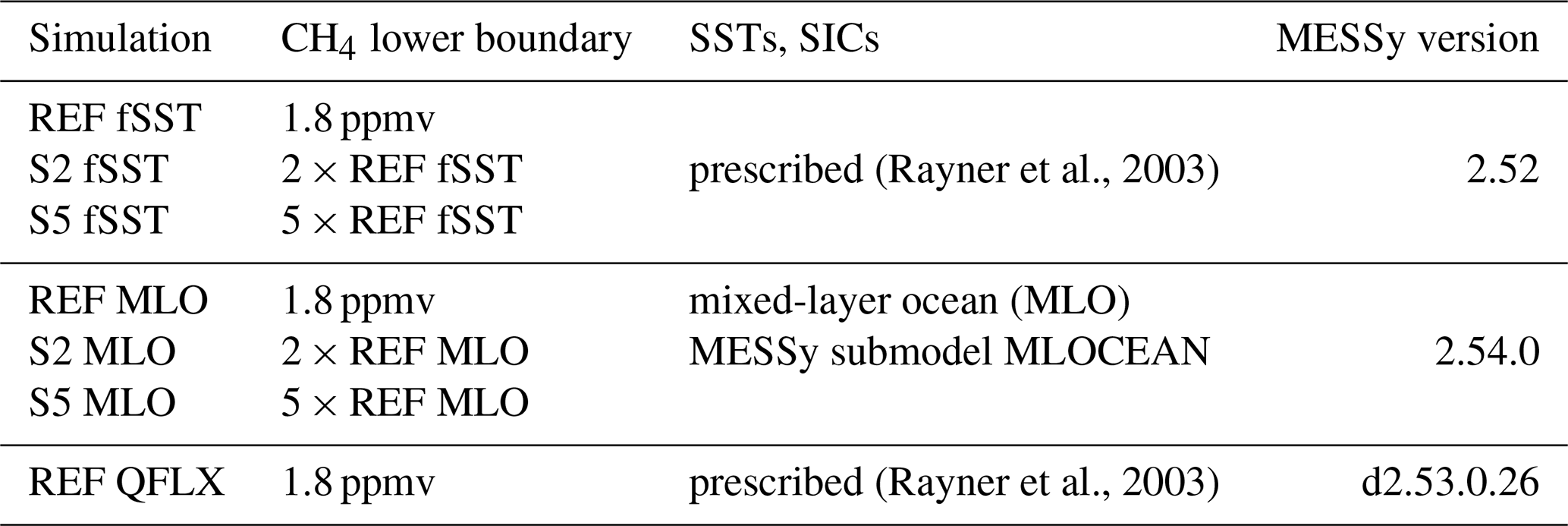
The MLO simulations have been initialized with the equilibrium CH4 fields of the respective fSST simulations. As the latter are already close to the respective equilibrium CH4 fields of the MLO simulations, the initialization with these fields shortens the spin-up. Like the fSST simulations, the CH4 lower-boundary mixing ratios of the MLO simulations are prescribed by Newtonian relaxation (i.e. nudging) with a nudging coefficient of 10 800 s. Thus, no CH4 emission flux boundary was used, but pseudo surface fluxes were calculated by the MESSy submodel TNUDGE (Kerkweg et al., 2006) to reach the prescribed CH4 lower-boundary mixing ratios. The lower-boundary CH4 mixing ratios of REF MLO are nudged to the same reference as REF fSST, namely an observation-based zonal mean estimate of the year 2010 from marine boundary-layer sites. The observational data are provided by the Advanced Global Atmospheric Gases Experiment (AGAGE; http://agage.mit.edu/, last access: 9 December 2020) and the National Oceanic and Atmospheric Administration Earth System Research Laboratory (NOAA-ESRL; https://www.esrl.noaa.gov/, last access: 9 December 2020). The lower-boundary CH4 mixing ratios of S2 and S5 are nudged towards the 2× and the 5× of this reference, respectively. The resulting global mean lower-boundary CH4 mixing ratio is about 1.8 parts per million volume (ppm) for both reference simulations, 3.6 ppm for both doubling, and 9.0 ppm for both quintupling experiments. Apart from CH4, all other boundary conditions and emission fluxes used in the sensitivity simulations are identical to the reference simulations and represent conditions of the year 2010 in general.
In the MLO simulations, the SSTs, the ice thicknesses, and the ice temperatures at ocean grid points are calculated by the MESSy submodel MLOCEAN. A MLO model accounts for the ocean's heat capacity without simulating the oceanic circulation explicitly. To simulate realistic SSTs with the MLO, a heat flux correction term needs to be added to the surface energy balance. We derived a monthly climatology of this heat flux correction from a control simulation with prescribed SSTs and SICs, named REF QFLX. REF QFLX uses the same monthly climatology of SSTs and SICs that was used for the fSST simulations, i.e. a monthly climatology representing the years 2000 to 2009 based on global analyses of the HadISST1 data set (Rayner et al., 2003).
In the following, the response to increased CH4 in the MLO simulations is assessed as the difference between either S2 MLO or S5 MLO and REF MLO. The effects of SST-driven climate feedbacks are identified as the difference between responses in the MLO and fSST simulations. The RIs induced by changes in individual radiatively active gases are assessed using the EMAC option for multiple radiation calls in the submodel RAD (Dietmüller et al., 2016), as explained in more detail by Winterstein et al. (2019). The first radiation call receives the reference mixing ratios of all chemical species, i.e. CH4, O3, and H2O. In the following radiation calls, each of the species individually and all combined are exchanged by climatological means derived from the sensitivity simulations (S2 and S5). From these perturbed radiation fluxes, the stratosphere adjusted RI is calculated (Stuber et al., 2001; Dietmüller et al., 2016).
3.1 Assessment of reference simulations
The simulation set-up of the reference simulation, REF MLO, aims to represent conditions typical for the year 2010. For a detailed assessment and evaluation of EMAC in general, we refer to Jöckel et al. (2016). We have evaluated the REF MLO CH4 mixing ratios to ensure that the latter represent conditions of 2010 sufficiently realistically. The REF MLO CH4 mixing ratios were compared to three different observational data sets that are independent from the observational estimate that serves as input for the lower boundary condition to ensure an objective evaluation. These are balloon-borne measurements conducted in the period from 1992 to 2006 from Röckmann et al. (2011), observations of a portable Fourier transform spectrometer on board the research vessel Polarstern during a cruise from Cape Town to Bremerhaven on the Atlantic in 2014 (Klappenbach et al., 2015), and observations from the Total Carbon Column Observing Network (TCCON; Wunch et al., 2011) from the period 2009 to 2014. The vertical profile, the north–south gradient and the annual cycle of REF MLO CH4 generally agree well with the corresponding data (not shown). Consistent with REF fSST (see Winterstein et al., 2019), there is a negative bias between the REF MLO and the observed total CH4 columns of less than 4 % (not shown). Note that not all the observations originate precisely from the year 2010. The global annual mean CH4 surface mixing ratios have, for example, risen by about 0.024 ppm from 2010 to 2014 (NOAA/ESRL; https://www.esrl.noaa.gov/gmd/ccgg/trends_ch4/, last access: 9 December 2020), the year of the study by Klappenbach et al. (2015). In addition, the CH4 lifetime could be slightly underestimated. The CH4 lifetime in EMAC lies in the middle to lower range in comparison with other CCMs (Jöckel et al., 2006; Voulgarakis et al., 2013). However, given that relative comparisons between sensitivity simulations and the reference are the main target of our analysis, REF MLO represents CH4 conditions of the year 2010 that are sufficiently realistic.
Since this study is one of the first to use the MLOCEAN submodel in MESSy, we have carefully checked whether REF MLO reproduces SSTs and SICs of the climatology that was used to determine the heat flux correction with sufficient accuracy. The spatial pattern of the SST climatology is realistically reproduced in REF MLO (see Fig. S1). The largest differences are found at higher latitudes, where a reduction in sea ice area leads to higher SSTs as exposed seawater is warmer than sea ice. REF MLO underestimates the monthly climatology of sea ice area in the Southern Hemisphere (SH) in all seasons, except for austral summer (see Fig. S2). The reduction in SIC results in up to 1.5 K higher SSTs in the Southern Ocean in REF MLO compared to the prescribed climatology (see Fig. S1). In the Northern Hemisphere (NH), the annual cycle of the sea ice area is generally well reproduced (see Fig. S2), except for a slight overestimation of the sea ice area in REF MLO, resulting in about 0.5 K lower annual mean SSTs in the Greenland Sea and in the Barents Sea (see Fig. S1). However, the sign of the global and annual mean surface temperature difference between REF MLO and REF fSST is determined by the positive REF MLO bias related to the Antarctic sea ice reduction. The global mean difference is 0.28 K, much less than the regional maxima near the ice edges, and with a small contribution of about 0.10 K from the tropical belt. It is unlikely that this will lead to substantial biases in the estimation of global mean surface temperature response and climate sensitivity in the intended equilibrium climate change simulations.
3.2 Tropospheric temperature response and associated climate feedbacks
The tropospheric temperature response to enhanced CH4 mixing ratios can freely develop in the MLO sensitivity simulations (see Fig. 1a, b). The temperature change patterns of S2 MLO and S5 MLO show the expected warming of the troposphere and cooling of the stratosphere (e.g. IPCC, 2013). The stratospheric cooling is less pronounced than in carbon dioxide (CO2)-driven climate change simulations since the CH4 cooling is mainly caused by associated O3 and H2O adjustments (Kirner et al., 2015; Winterstein et al., 2019). Maximum warming in polar regions and in the upper tropical troposphere is also consistent with changes expected from increased levels of GHGs (e.g. Chap. 12 in IPCC, 2013). CH4 doubling (quintupling) leads to temperature increases of up to 1 K (3 K) in the Arctic on annual average. Antarctica also warms up particularly strongly in the S5 MLO scenario, with a maximum warming of up to 3 K. As a result of the especially strong warming in polar regions, the sea ice area is reduced in both sensitivity simulations with respect to the reference (compare Fig. S2).

Figure 1(a, b) Absolute annual zonal mean temperature differences between the sensitivity simulations (a) S2 MLO and (b) S5 MLO and REF MLO in kelvin. (c, d) Differences between the temperature response to enhanced CH4 in the MLO and fSST set-ups in kelvin. To calculate the latter, the absolute changes in (c) S2 fSST and (d) S5 fSST are subtracted from the absolute changes in S2 MLO and S5 MLO, respectively. Non-stippled areas are significant on the 95 % confidence level according to a two-sided Welch's test. The solid black line indicates the climatological tropopause height of REF MLO.
The Brewer–Dobson circulation (BDC) is expected to accelerate in a warming climate (Rind et al., 1990; Butchart and Scaife, 2001; Garcia and Randel, 2008; Butchart, 2014; Eichinger et al., 2019). Feedbacks on the chemical composition of the atmosphere, especially of the stratosphere, which result from changes in the BDC are of particular interest in this study as they will modify the mainly chemically induced changes discussed by Winterstein et al. (2019). The BDC influences the spatial distribution of trace gases, such as O3, H2O, and CH4, in the stratosphere and also their transport from the troposphere into the stratosphere (Butchart, 2014). In Fig. 2 we examine the response of the residual mean streamfunction to quantify changes in the BDC. There is indeed a strengthening of the residual mean circulation in both, S2 MLO and S5 MLO, with respect to REF MLO and it is detected in both hemispheres. The change in the residual mean streamfunction is stronger and extends to higher altitudes for the simulation S5 MLO, but the annual mean patterns are consistent in both MLO sensitivity simulations. The maximum change of about 0.7×10⁹ kg s−1 for S5 MLO is located at about 100 hPa. Upward motion is increased in the tropics, which is balanced by an increase in downwelling between 30–60∘ latitude in both hemispheres. The change in the residual mean streamfunction is stronger and reaches higher altitudes in the respective winter hemisphere in S5 MLO (see Figs. S3 and S5). The BDC response in the MLO simulations is considerably stronger than in the respective fSST sensitivity simulations. This is expected since the main driver of changes in the BDC is tropospheric warming (Butchart, 2014). We note that changes in the residual mean streamfunction below the tropical tropopause in response to CH4 increase exhibit different patterns in the fSST and MLO simulations (see Fig. 2). Differences between the fast and the slow response of the tropospheric tropical circulation have been noticed and discussed in CO2 increase simulations, too (e.g. Bony et al., 2013). However, trying to explain the origin of these tropospheric differences would be beyond the scope of the present paper, which focuses on stratospheric trace gas feedbacks to CH4 increase. The latter are influenced by the more distinct strengthening of the BDC in the MLO experiments, as we show in the next section.
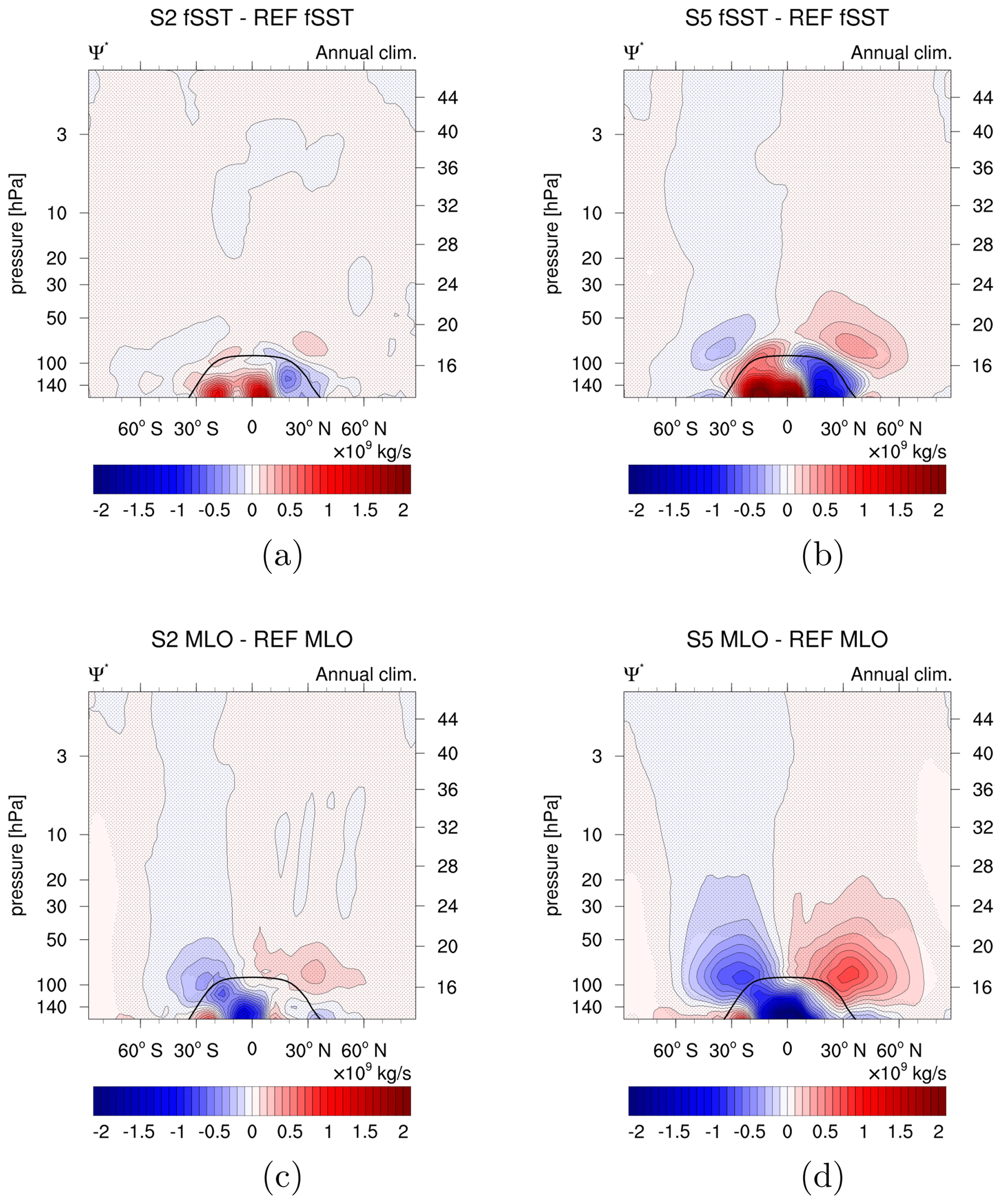
Figure 2Absolute differences in the annual zonal mean residual streamfunction between the sensitivity simulations (a) S2 fSST, (b) S5 fSST, (c) S2 MLO, and (d) S5 MLO compared to their respective reference in 109 kg s−1. Non-stippled areas are significant on the 95 % confidence level according to a two-sided Welch's test. The solid black line indicates the climatological tropopause height of REF MLO.
3.3 Influence of interactive SSTs
3.3.1 Chemical composition
Winterstein et al. (2019) analysed the quasi-instantaneous impact of doubled and quintupled CH4 mixing ratios on the chemical composition of the atmosphere. In this section we investigate the respective slow feedbacks that are assessed as the difference between the full response (as simulated in the MLO simulations) and the rapid adjustments (as simulated in the fSST simulations). The slow feedbacks are therefore visualized as the differences between the response patterns in the fSST simulations and in the MLO simulations.
Tropospheric CH4 lifetime and OH
The oxidation with OH is the most important sink of CH4 in the troposphere (e.g. Saunois et al., 2016a). The amount of oxidized CH4 affects the OH mixing ratios as the reaction consumes OH, which in turn feeds back on the atmospheric CH4 lifetime. In this study, consistent with Winterstein et al. (2019), the CH4 lifetime is calculated according to Jöckel et al. (2016) as
with being the mass of CH4 [kg], the temperature dependent reaction rate coefficient of the reaction CH4 + OH → products [cm3 s−1], cair the concentration of air [cm−3], and xOH the mole fraction of OH [mol mol−1] in all grid boxes b ∈ B. B is the region for which the lifetime should be calculated, e.g. all grid boxes below the tropopause for the mean tropospheric lifetime. For the CH4 lifetime calculation a climatological tropopause, defined as tpclim=300–215 hPa ⋅ cos2(ϕ), with ϕ being the latitude in degrees north, is used as recommended by Lawrence et al. (2001).
Figure 3 shows the mean tropospheric CH4 lifetime of the MLO experiments, together with the fSST experiments, dependent on the CH4 scaling factor, i.e. 1 for the reference simulations, 2 for the experiments with 2×CH4, and 5 for those with 5×CH4. An almost linear relationship between the mean tropospheric CH4 lifetime and the CH4 scaling factor is present also in the MLO sensitivity simulations. The lifetime increase is, however, reduced by 0.30 a (increase by 2.03 a instead of 2.3 a) and 1.17 a (increase by 6.37 a instead of 7.54 a) in the MLO set-up compared to fSST when doubling and quintupling CH4, respectively. This weaker increase is in line with a weaker decrease in tropospheric OH in the MLO sensitivity simulations compared to fSST as obvious from Fig. 4c, d, which show the difference between the OH response in the MLO and in the fSST sensitivity simulations. In the troposphere this difference is hardly significant anywhere for the 2×CH4 experiments, whereas it is significant in the tropics for 5×CH4. The weaker decrease in tropospheric OH in both MLO simulations is related to more strongly enhanced OH precursors (H2O and O3) in the troposphere in the MLO compared to the fSST sensitivity simulations, as is discussed below. Additionally, the tropospheric warming in the MLO sensitivity simulations results in a faster CH4 oxidation as its reaction rate increases with temperature. The isolated effect of the temperature-dependent reaction rate is indicated by the blue squares in Fig. 3. They show the CH4 lifetime corresponding to REF MLO conditions, except for the reaction rate coefficient that was calculated with temperatures corresponding to 2× and 5×CH4.
Voulgarakis et al. (2013) compared the CH4 lifetime increase simulated in two simulations: one with the full RCP8.5 climate change signal of the year 2100 with respect to 2000 and one with CH4 concentrations corresponding to 2100 RCP8.5 levels but climate conditions of the year 2000. They identified a weaker increase in the CH4 lifetime with tropospheric warming as well. Their difference is larger than the difference between the S2 fSST and S2 MLO lifetime responses even though the CH4 increase simulated by Voulgarakis et al. (2013) is of the same order of magnitude as in S2 fSST and S2 MLO since the RCP8.5 scenario projects a doubling of the 2010 CH4 mixing ratios at the end of the century. However, the tropospheric warming in the RCP8.5 scenario is stronger because it includes the effects of all GHGs as opposed to the isolated effect of CH4 in our experiments. Additional warming induced by other GHGs, in particular CO2, would drive H2O and O3 increases as well. Therefore, the reduction in OH driven by CH4 increases in our experiments is expected to be more strongly offset under a simultaneously active CO2 forcing.
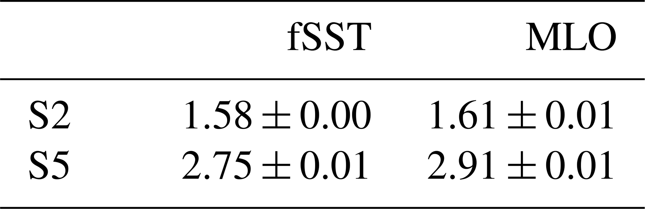
Please recall that we prescribe the CH4 mixing ratios at the lower boundary using Newtonian relaxation. It is important to note that the prolongation of the tropospheric CH4 lifetime causes the corresponding CH4 fluxes at the lower boundary to not scale equally with the mixing ratio increase but to increase by a smaller factor. Increasing the CH4 surface mixing ratio by a factor of 2 (5) corresponds to an increase in the CH4 surface fluxes by a factor of 1.61 ± 0.01 (2.91 ± 0.01) in the MLO simulations and by a factor of 1.58 ± 0.00 (2.75 ± 0.01) in the fSST simulations (see Table 2). The larger increase factors in the MLO sensitivity simulations are in line with the reduced prolongation of the tropospheric CH4 lifetime compared to the fSST experiments. The fact that the increase in emission fluxes is less than a factor of 2 or 5 suggests that enhanced CH4 emissions would likewise scale the mixing ratio by a larger factor than the corresponding increase factor of the emissions. The CH4 surface fluxes that result from the nudging of the mixing ratio towards zonally averaged CH4 fields are not realistic in terms of spatial distribution, however.

Figure 3Mean tropospheric CH4 lifetime with respect to the oxidation with OH versus the scaling factor of the lower-boundary CH4, i.e. 1 for REF, 2 for S2, 5 for S5 for the MLO (red, dashed) and the fSST (black, solid) simulations. In addition, the isolated effect of the temperature-dependent reaction rate is shown for the MLO experiments (blue squares). The horizontal lines indicate the 95 % confidence intervals based on annual mean values of the CH4 tropospheric lifetime.

Figure 4(a, b) Relative differences between the annual zonal mean OH mixing ratios of the sensitivity simulations (a) S2 MLO and (b) S5 MLO and REF MLO (%). (c, d) Differences between the OH response to enhanced CH4 in the MLO and fSST set-ups (percentage points). To calculate the latter, the relative changes in (c) S2 fSST and (d) S5 fSST are subtracted from the relative changes in S2 MLO and S5 MLO, respectively. Non-stippled areas are significant on the 95 % confidence level according to a two-sided Welch's test. The solid black line indicates the climatological tropopause height of REF MLO.
Table 2Increase factors of the global mean CH4 surface fluxes, which correspond to increases in the CH4 mixing ratios by factors of 2 or 5, respectively. The values after the ± sign are the 95 % confidence intervals of the mean calculated using Taylor expansion (assuming REF fluxes to be uncorrelated with either S2 or S5 fluxes) as , with the mean fluxes of either S2 or S5 and REF and , respectively; interannual standard deviations sx and sy; number of analysed years Nx and Ny; α=0.05; and the degrees of freedom .
Non-linearities of CH4 increase
Figure 5 shows the relative differences between the annual zonal mean CH4 of S2 MLO (S5 MLO) and 2× (5×) the zonal mean CH4 of REF MLO. The doubling or quintupling of the reference CH4 serves to emphasize regions where the increase factor of the CH4 mixing ratio deviates from 2 or 5, respectively. The response of tropospheric CH4 is marginally larger than a linear increase in both MLO experiments. This is in line with the response of tropospheric CH4 in the fSST simulations. Tropospheric CH4 is largely controlled by the nudging at the lower boundary through mixing and is, therefore, prevented from adjusting to the lifetime increase as discussed above. The slightly positive values in Fig. 5 indicate a small residual of this effect. As for the fSST simulations, the CH4 increase between 50 and 1 hPa is smaller than the factors of 2 or 5, respectively. This effect is less pronounced in the two MLO sensitivity experiments compared to the respective fSST experiments (compare with Fig. 3 in Winterstein et al., 2019), suggesting that the chemical depletion of CH4 is enhanced in the MLO experiments as well, however, less strongly than in the fSST experiments.
Another aspect to note in Fig. 5 is the more than 2× or 5×CH4 increase in the lowermost tropical stratosphere. This feature indicates enhanced tropical upwelling, which leads to larger CH4 mixing ratios in the tropical lower stratosphere. It is more pronounced in the MLO than in the fSST experiments, in line with the more pronounced changes in tropical upwelling in the MLO set-up as discussed in Sect. 3.2. The average deviation from 2× or 5×CH4 for a region in the tropical lower stratosphere (30–30∘ N, 70–20 hPa) is 0.16 % for S2 fSST, 0.37 % for S2 MLO, 0.23 % for S5 fSST, and 1.31 % for S5 MLO. Furthermore, strengthening of the BDC transports CH4 more efficiently to higher altitudes, leading to higher CH4 mixing ratios there as well. This can be one explanation for the weaker deviation from a linear CH4 increase in the MLO compared to the fSST simulations. Another explanation, as already stated, is that the chemical depletion of CH4 is less strongly enhanced in the MLO sensitivity simulations compared to fSST. We therefore discuss differences in the response of OH, the most important sink partner of CH4, in the next paragraph.
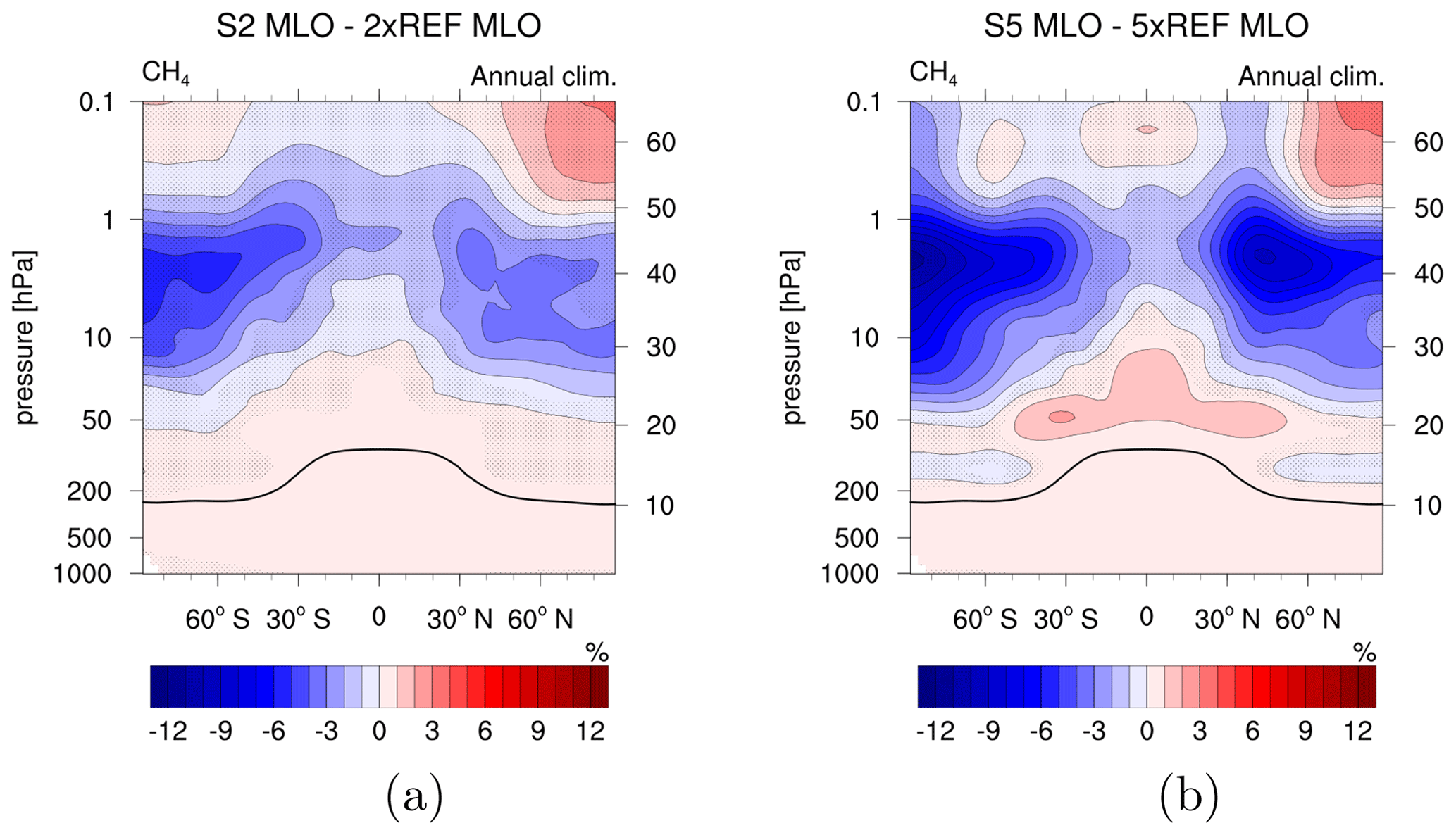
Figure 5Relative differences between the annual zonal mean CH4 of the sensitivity simulations (a) S2 MLO and 2× REF MLO and (b) S5 MLO and 5× REF MLO (%). Non-stippled areas are significant on the 95 % confidence level according to a two-sided Welch's test. The solid black line indicates the climatological tropopause height of REF MLO.
Stratospheric OH mixing ratios increase in both simulation set-ups (fSST and MLO) on the order of 30 % for 2×CH4 and 60 %–80 % for 5×CH4 (see Fig. 4 in Winterstein et al., 2019, for fSST and Fig. 4a, b for MLO). The OH increase in the stratosphere is weaker in the MLO simulations compared to the fSST simulations (see Fig. 4c, d). The differences are, however, small compared to the total increase in OH and mainly not significant. The difference between the two 5×CH4 experiments reaches up to 5 percentage points (p.p.) in the middle stratosphere. The weaker increases in OH are presumably connected to weaker increases in SWV in the MLO simulations. The considerably weaker OH increase above the tropical tropopause in S5 MLO with respect to S5 fSST is possibly associated with a stronger O3 decrease in this area in S5 MLO. Changes in both SWV and O3 are discussed below. The weaker OH increases in the MLO sensitivity experiments with respect to fSST are in line with the smaller deviations from a linear doubling or quintupling of the CH4 mixing ratio in the stratosphere (see Fig. 5). We conclude that the strengthening of the CH4 oxidation resulting from increases in the OH mixing ratio is weaker in the MLO experiments but still present.
Water vapour
Winterstein et al. (2019) reported a steady increase in SWV with height for the fSST experiments as an outcome of the enhanced CH4 depletion as discussed in the previous paragraph, whereas tropospheric H2O remained largely unaffected. The warming of the troposphere in the MLO simulations consistently leads to an increase in the H2O mixing ratios also in the troposphere as evident from Fig. 6. The maximum difference in tropospheric H2O response between MLO and fSST can be found in the upper tropical troposphere and extratropical lowermost stratosphere and reaches 11 p.p. (35 p.p.) for the 2× (5×) CH4 experiments.
In the middle and upper stratosphere, the H2O increase is about 5 p.p. (15 p.p.) weaker in the S2 MLO (S5 MLO) sensitivity simulation compared to S2 fSST (S5 fSST). This reduction is significant but small compared to the relative increase in SWV of around 50 % for both 2×CH4 and 250 % for both 5×CH4 experiments. The amount of tropospheric H2O transported into the stratosphere is largely determined by the cold point temperature (CPT) (e.g. Randel and Park, 2019). Furthermore, the oxidation of CH4 is an important in situ source of SWV (Hein et al., 2001; Rohs et al., 2006; Frank et al., 2018). The SWV mixing ratio at a given location and time can be approximated as the sum of these two terms following Austin et al. (2007) and Revell et al. (2016) as
We calculate the amount of tropospheric H2O entering the stratosphere as the tropical (10∘ S–10∘ N) mean H2O mixing ratio at 70 hPa following Revell et al. (2016). The H2O entry mixing ratio increases by 9.08 % (0.14 ppm) in S2 fSST, 9.77 % (0.17 ppm) in S2 MLO, 38.53 % (0.57 ppm) in S5 fSST, and 38.86 % (0.68 ppm) in S5 MLO. Furthermore, the zonal mean tropical CPT increases in all sensitivity simulations (see Fig. S7). Though differences exist between the reference CPT in MLO und fSST, the magnitude and latitudinal structure of the CPT changes are very similar for both doubling and both quintupling experiments. They are also a bit larger for the MLO experiments (again consistent for the S2 and S5 case), in line with the response of the H2O entry mixing ratios. Changes in the amount of tropospheric H2O entering the stratosphere can therefore not explain the weaker increase in SWV in the MLO experiments compared to fSST in the middle and upper stratosphere.
To illustrate the effect of CH4 oxidation on the SWV response, Fig. S8 shows the response of H2O from CH4 oxidation estimated using Eq. (2). As discussed in the previous paragraph, the strengthening of the CH4 oxidation in the stratosphere is weaker in the MLO experiments. This results in a weaker increase in SWV produced by CH4 oxidation in the middle and upper stratosphere (see Fig. S8c, d) and can explain the difference in SWV response between MLO and fSST as shown in Fig. 6c, d.
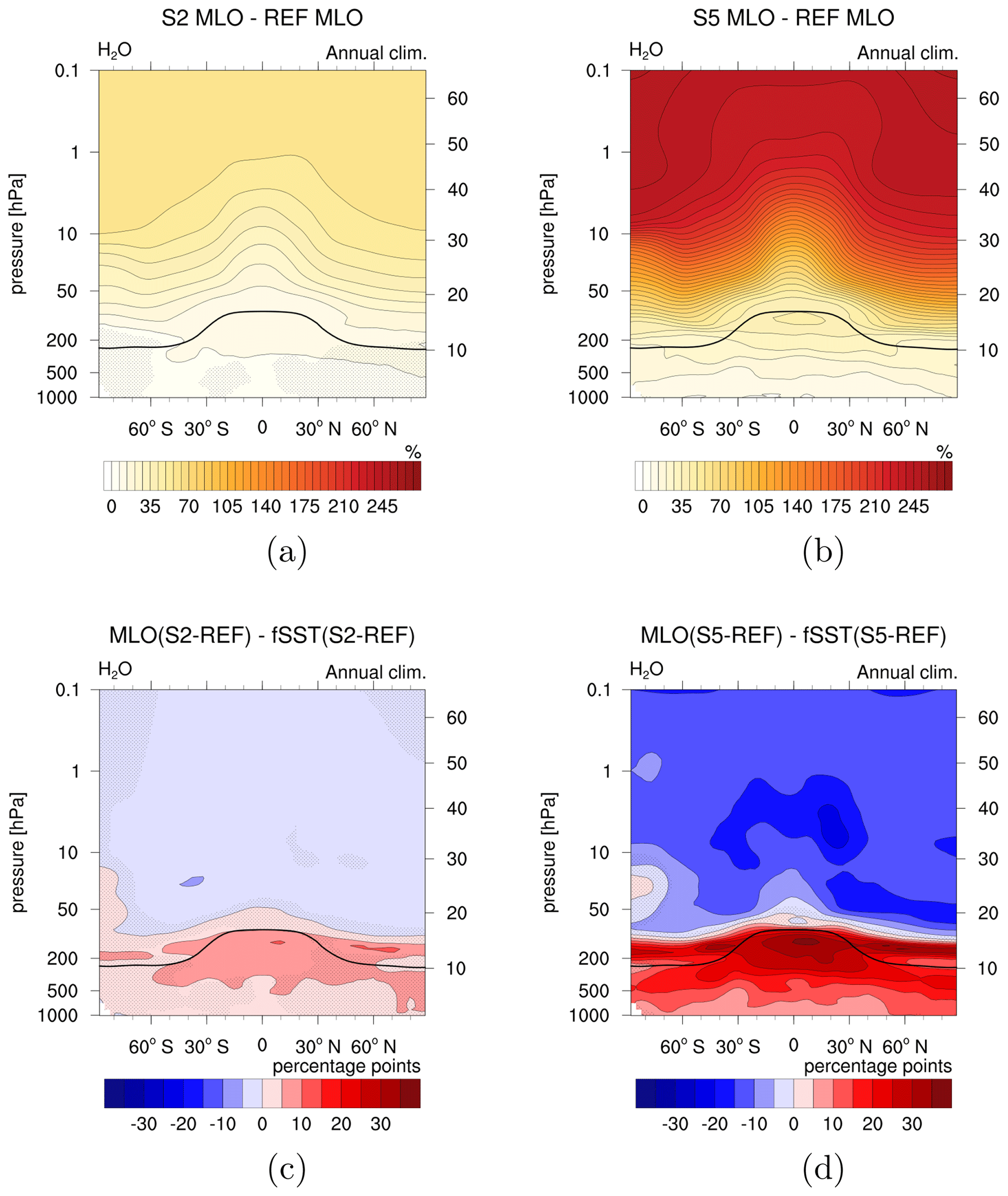
Figure 6(a, b) Relative differences between the annual zonal mean H2O mixing ratios of the sensitivity simulations (a) S2 MLO and (b) S5 MLO and REF MLO (%). (c, d) Differences between the H2O response to enhanced CH4 in the MLO and fSST set-ups (percentage points). To calculate the latter, the relative changes in (c) S2 fSST and (d) S5 fSST are subtracted from the relative changes in S2 MLO and S5 MLO, respectively. Non-stippled areas are significant on the 95 % confidence level according to a two-sided Welch's test. The solid black line indicates the climatological tropopause height of REF MLO.
What remains to be explained is the reason for the weaker strengthening of the CH4 oxidation in the MLO set-up compared to fSST. Strengthened tropical upwelling as shown in Sect. 3.2 transports CH4 into the stratosphere more efficiently and would be expected to lead to higher rates of the CH4 oxidation (Austin et al., 2007). However, as the strengthening of the CH4 oxidation is weaker in the MLO experiments, CH4 itself seems not to be the limiting factor here. The abundance of SWV feeds back on OH and therefore also on the efficiency of the CH4 oxidation. However, the increase in SWV seems to be rather a result of the strengthened CH4 oxidation here as the increase in H2O entering the stratosphere is higher in the MLO experiments compared to fSST.
Ozone
The other important precursor of OH is O3, the abundance of which is also influenced by CH4. The stratospheric O3 response pattern in the MLO experiments, namely O3 reduction in the lowermost tropical stratosphere, O3 increase up to approximately 2 hPa, and O3 decrease above, is qualitatively consistent with the fSST simulations (compare Fig. 7 in Winterstein et al., 2019, and Fig. 7a, b). Winterstein et al. (2019) gave a detailed explanation of the processes leading to the resulting O3 pattern that is also valid for the MLO simulations. As the O3 catalytic depletion cycles are less efficient at lower temperatures, radiative cooling in the stratosphere results in increased O3 mixing ratios in the middle stratosphere (between 50 and 5 hPa). Additionally, increased abundances of H2O favour the depletion of excited oxygen (O(1D)), likewise reducing the sink of O3 and favouring increases in the O3 abundance. Reduced O3 mixing ratios in the lowermost tropical stratosphere indicate enhanced tropical upwelling of O3-poor air from the troposphere into the stratosphere. Above 2 hPa, increases in OH lead to enhanced depletion of O3, resulting in reduced O3 mixing ratios.
When subtracting the fSST response from the MLO response, the extra effect of tropospheric warming becomes apparent. The resulting patterns for S2 and S5 are shown in Fig. 7c, d. A dominant feature is the stronger decrease in O3 in the lowermost tropical stratosphere in S5 MLO compared to S5 fSST of up to 18.39 p.p. The average difference between S5 MLO and S5 fSST for a region in the tropical lower stratosphere (30∘ S–30∘ N, 100–20 hPa) is 6.33 p.p. This difference also exists between the S2 simulations, albeit weaker (with a maximum difference of 4.68 p.p. and an average difference of 1.67 p.p.). The more strongly decreasing O3 mixing ratios in MLO indicate that the transport of O3-poor air from the troposphere into the stratosphere is intensified in the MLO simulations. The increases in O3 in the southern polar middle stratosphere in S2 MLO and in both polar regions in S5 MLO are more pronounced with respect to the respective fSST experiment. This indicates more strongly enhanced meridional transport in the MLO experiments. Both patterns are in line with the strengthening of the residual mean circulation as discussed in Sect. 3.2.
In the tropospheric O3 response pattern (shown in Fig. 7a, b), any O3 feedback from tropospheric warming is superimposed by chemical influences of CH4. Therefore, the pattern is fundamentally different from O3 changes in global warming simulations driven by CO2 increases (see Fig. 1a in Dietmüller et al., 2014; Fig. 3a in Nowack et al., 2018; and Fig. 1a–c in Chiodo and Polvani, 2019), where direct chemical impacts are weak. However, if the O3 response to slow climate feedbacks induced by enhanced CH4 is separated from rapid adjustments (Fig. 7c, d), a similar pattern to the O3 response induced by enhanced CO2 arises. An exception is the increase in O3 above 30 hPa that results from a slower chemical depletion of O3 caused by stratospheric radiative cooling (Dietmüller et al., 2014), which develops on the timescale of rapid radiative adjustments. A deceleration of the chemical O3 destruction in the middle stratosphere is also present in the CH4-driven experiments, resulting mainly from radiative cooling induced by adjustments of SWV and O3 (see Fig. 8e and f in Winterstein et al., 2019), but cancels out in Fig. 7c, d.
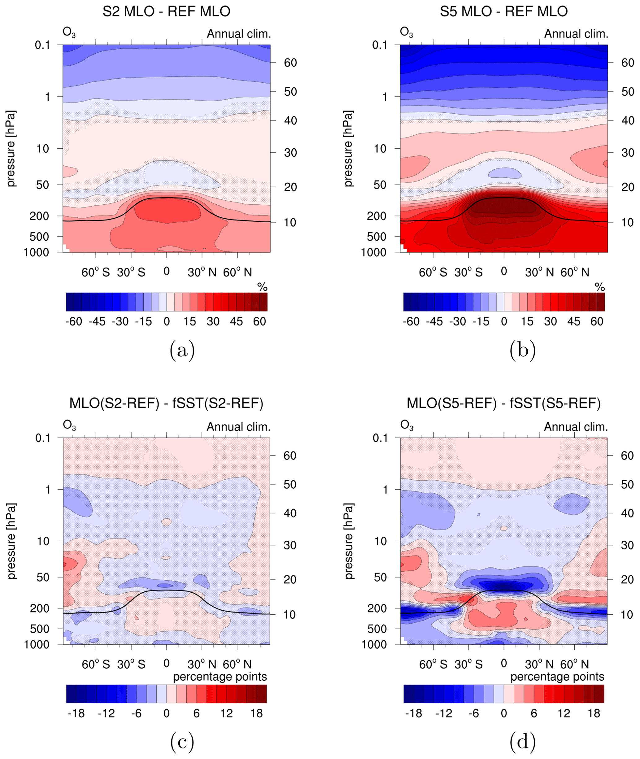
Figure 7(a, b) Relative differences between the annual zonal mean O3 mixing ratios of the sensitivity simulations (a) S2 MLO and (b) S5 MLO and REF MLO (%). (c, d) Differences between the O3 response to enhanced CH4 in the MLO and fSST set-ups (percentage points). To calculate the latter, the relative changes in (c) S2 fSST and (d) S5 fSST are subtracted from the relative changes in S2 MLO and S5 MLO, respectively. Non-stippled areas are significant on the 95 % confidence level according to a two-sided Welch's test. The solid black line indicates the climatological tropopause height of REF MLO.
3.3.2 Radiative impact, surface temperature response, and climate sensitivity
In Winterstein et al. (2019) the total RI has been separated into the individual contributions of the species CH4, SWV, and O3, an analysis we extend hereafter to the MLO simulations. Note that we adopt the definition of Winterstein et al. (2019) concerning the RI, which indicates the radiative flux imbalance between the sensitivity and the reference simulation.
In Table 3 we summarize the RI of the most important species in both the fSST and the MLO simulations. The individual contributions to the RI have been calculated with the submodel RAD (Dietmüller et al., 2016) in separate simulations (S2 fSST∗, S5 fSST∗, S2 MLO∗, and S5 MLO∗; see Sect. 2). We further separate the H2O and O3 contribution into tropospheric and stratospheric RI, respectively. The RIs of CH4 and O3 show only small differences between fSST and MLO. This implies that SST-driven climate feedbacks on these constituents do not substantially alter their RI contribution in our simulation set-up. As expected, the RI of tropospheric H2O increases substantially. The RI of stratospheric H2O increases as well, which is mostly influenced by the increase in SWV in the lowermost stratosphere due to transport of moist air from the tropical troposphere into the stratosphere (see Fig. 6).
The global mean surface temperature responses in the MLO experiments for 2× and 5×CH4 are 0.42±0.05 K and 1.28±0.04 K, respectively. The forcing strengths of 2× and 5×CH4 turn out too small to robustly quantify the corresponding climate sensitivity parameters λ with a sensitivity analysis of the entire transient data following Gregory et al. (2004). Therefore, we calculate λ, under the reasonable assumption that the total RIs from the fSST experiments represent the corresponding ERFs with chemical rapid adjustments included (Winterstein et al., 2019), as 0.61 ± 0.17 and 0.72 ± 0.07 K W−1 m2, respectively. The estimate of λ corresponding to 5×CH4 compares well with the climate sensitivity parameter λadj of 0.73 K W−1 m2 from Rieger et al. (2017) corresponding to a 1.2 × CO2 experiment with EMAC with an RF of 1.06 W m−2, which is comparable to the RIs in the present experiments. The agreement of the climate sensitivity parameters for CH4 and CO2 forcing suggests an efficacy of CH4 ERF close to 1. The estimate of λ for 2×CH4 is smaller than the value from Rieger et al. (2017), but the difference is insignificant as a consequence of large statistical uncertainty.
In a recent multimodel comparison, the multimodel mean efficacy of CH4 was found to be smaller than unity, however, with a large inter-model spread ranging from 0.56 to 1.15 (Richardson et al., 2019). Modak et al. (2018) found a CH4 efficacy of 0.81 for a simulation with a CH4 increase comparable to S5. They identified CH4 shortwave (SW) absorption and related warming of the lower stratosphere and upper troposphere as reasons for the CH4 efficacy value slightly below unity. Our simulation set-up does not account for SW absorption of CH4. The climate sensitivity and efficacy estimates of Modak et al. (2018) and Richardson et al. (2019) do not include chemical feedbacks of O3 and SWV induced by CH4. They also do not provide a robust indication that the CH4 efficacy is significantly larger or smaller than unity in their framework as the inter-model spread reported by Richardson et al. (2019) is so large. Estimating a reasonable climate sensitivity value from our simulations in an interactive chemistry framework requires that rapid adjustments from SWV and O3 are included in the effective CH4 forcing. If this is done, these simulations do not point at a significant climate sensitivity deviation from the CO2 behaviour either.
Table 3An estimation of individual RI contributions [W m−2] of the changes in the chemical species CH4, H2O, and O3. Values are calculated using the RAD submodel (Dietmüller et al., 2016) in separate simulations (S2 fSST∗, S5 fSST∗, S2 MLO∗, and S5 MLO∗; see Sect. 2) using 20-year climatologies of the individual species from the corresponding reference and sensitivity simulation experiments fSST and MLO. The lower part shows the global mean 2 m air temperature changes of S2 MLO and S5 MLO with respect to REF MLO and the total RIs of S2 fSST and S5 fSST. From these temperature changes and total RIs, the climate sensitivity parameter λ is calculated as λ=ΔTMLO ∕ total RIfSST.
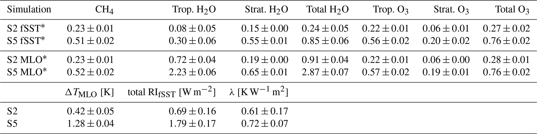
The values after the ± sign are the 95 % confidence intervals of the mean. For λ the confidence intervals are calculated using Taylor expansion and assuming ΔTMLO and total RIfSST to be uncorrelated as , with the mean values of ΔTMLO and total RIfSST and , respectively; interannual standard deviations sx and sy; number of analysed years Nx and Ny; α=0.05; and the degrees of freedom .
3.3.3 Radiatively and dynamically driven atmospheric temperature response
The two lower panels in Fig. 1 show the differences in temperature response between the MLO and the fSST simulations. As expected, tropospheric warming is significantly stronger in the MLO experiments since the tropospheric temperature change is largely suppressed in the simulations with prescribed SSTs and SICs. In the stratosphere, radiatively and dynamically driven effects contribute to differences in the temperature change patterns between MLO and fSST, as is shown in the following. Note again that changes in the chemical composition resulting from a change in circulation (i.e. transport) are included in the radiatively driven effects by our definition.
Following Winterstein et al. (2019) we calculate the stratosphere adjusted temperature response ΔTadj to changes in CH4, tropospheric and stratospheric H2O, and tropospheric and stratospheric O3 as well as their individual contributions for S2 MLO and S5 MLO (see Fig. S9 for simulation S2 MLO and Fig. 8 for simulation S5 MLO). ΔTadj represents the temperature response induced by changes in the composition of radiatively active gases (Stuber et al., 2001). The difference in ΔTadj between S5 MLO and S5 fSST is shown in Fig. 9 (for S2 see Fig. S10). This difference is small for CH4 and tropospheric O3 (see Fig. 9b, g). Figure 9d confirms the stratospheric radiative cooling effect of increased humidity in the troposphere in S5 MLO, although the effect is quantitatively small. The stratosphere adjusted temperature response pattern induced by SWV in S5 MLO is similar to S5 fSST. However, the stronger increases of SWV in S5 MLO result in more pronounced cooling in the lowermost stratosphere, whereas the reduced increases above consistently result in reduced cooling (see Fig. 9e). The stronger decrease in O3 in the tropical lower stratosphere in S5 MLO (see Fig. 7) leads to stronger cooling in this region as shown in Fig. 9h. These results also apply qualitatively to the comparison of S2 MLO and S2 fSST (see Fig. S10), but the magnitude of the differences is smaller. The effects from SWV and stratospheric O3 dominate the differences in ΔTadj between S5 MLO and S5 fSST (compare Fig. 9a). In addition, the resulting more pronounced cooling in the lowermost stratosphere in the MLO simulations is apparent in the difference between the overall temperature responses of MLO and fSST in Fig. 1c, d.
By calculating the difference between the total temperature response in the regular simulations ΔT and the sum of the individual contributions of CH4, H2O, and O3 to the stratosphere adjusted temperatures (; see Figs. 8a and S9a), we attempt to identify the dynamical effect () in the stratosphere temperature response as
with X being either 2 or 5. A similar approach was used by, for example, Rosier and Shine (2000) and Schnadt et al. (2002) to distinguish between the radiative impact of trace gases and dynamical contributions to the total temperature response.
Figure 10 shows the annual mean of for all four sensitivity simulations. It is mostly not significant for S2 fSST and S5 fSST in the stratosphere, suggesting that dynamical effects play a minor role in the temperature response in these simulations as already indicated by Winterstein et al. (2019). However, immediately above the tropical tropopause centred at the Equator indicates warming for both, S2 fSST and S5 fSST. In austral winter (JJA), shows significant cooling in the southern polar stratosphere for S2 fSST and S5 fSST. The cooling extends into austral spring (SON) but gradually weakens as time proceeds (see Figs. S13 and S14). These temperature changes can be associated with the strengthening of the SH stratospheric winter polar vortex (see Fig. S16), which leads to enhanced isolation of air masses and stronger cooling. The stratospheric polar vortex in boreal winter (DJF) accelerates in both fSST sensitivity simulations as well (see Fig. S15).
The pattern of for S5 MLO (Fig. 10d) displays a near-symmetrical behaviour around the Equator. It comprises two warming patches in the lower stratosphere – unlike S5 fSST not centred at the Equator but at around 30∘ S or 30∘ N – as well as cooling in the tropics and warming in the extratropics in the middle stratosphere. The warming patches in the lower stratosphere are present in all seasons, whereas the pattern of cooling in the tropics and warming in the extratropics above is shifted to the respective winter hemisphere (compare Figs. S11 and S13). For S2 MLO, the warming patches in the lower stratosphere are also present in the pattern of . Apart from that, the annual mean is mostly not significant for S2 MLO. However, the pattern of cooling in the tropics and warming in the extratropics is indicated in boreal autumn (SON) and winter (DJF) for S2 MLO as well.
We associate the main component of the pattern of the MLO experiments with the strengthening of the BDC as discussed in Sect. 3.2. Strengthened downwelling in the subtropical and extratropical lower stratosphere results in adiabatic warming in this region in both hemispheres throughout the year. These temperature changes can therefore be associated with the intensification of the shallow branch of the BDC (Plumb, 2002; Birner and Bönisch, 2011). The patterns are present in S2 MLO and S5 MLO. Adiabatic cooling in the tropical middle and upper stratosphere as well as a respective adiabatic warming in the extratropical and polar winter stratosphere indicates the strengthening of the deep branch of the BDC, more pronounced in S5 MLO than in S2 MLO. The strengthening of the BDC would be expected to result in adiabatic cooling directly above the tropopause from increased tropical upwelling. This effect seems to be masked by other processes in Fig. 10. These could be advection or mixing of warm air from the troposphere or increased longwave (LW) radiation from the warmer troposphere and potentially more LW absorption in the lowest stratosphere. Lin et al. (2017) found the latter effect to cause strong warming in the tropical tropopause layer. This radiative effect is not accounted for in , which is the sum of the individual contributions of radiatively active gases to the stratosphere adjusted temperatures. Furthermore, mixing with air out of the upper tropical troposphere could also contribute to the warming patches in the subtropical and extratropical lower stratosphere. This region is particularly affected by mixing (Dietmüller et al., 2018; Eichinger et al., 2019), and mixing itself can also be influenced by climate change (Eichinger et al., 2019).
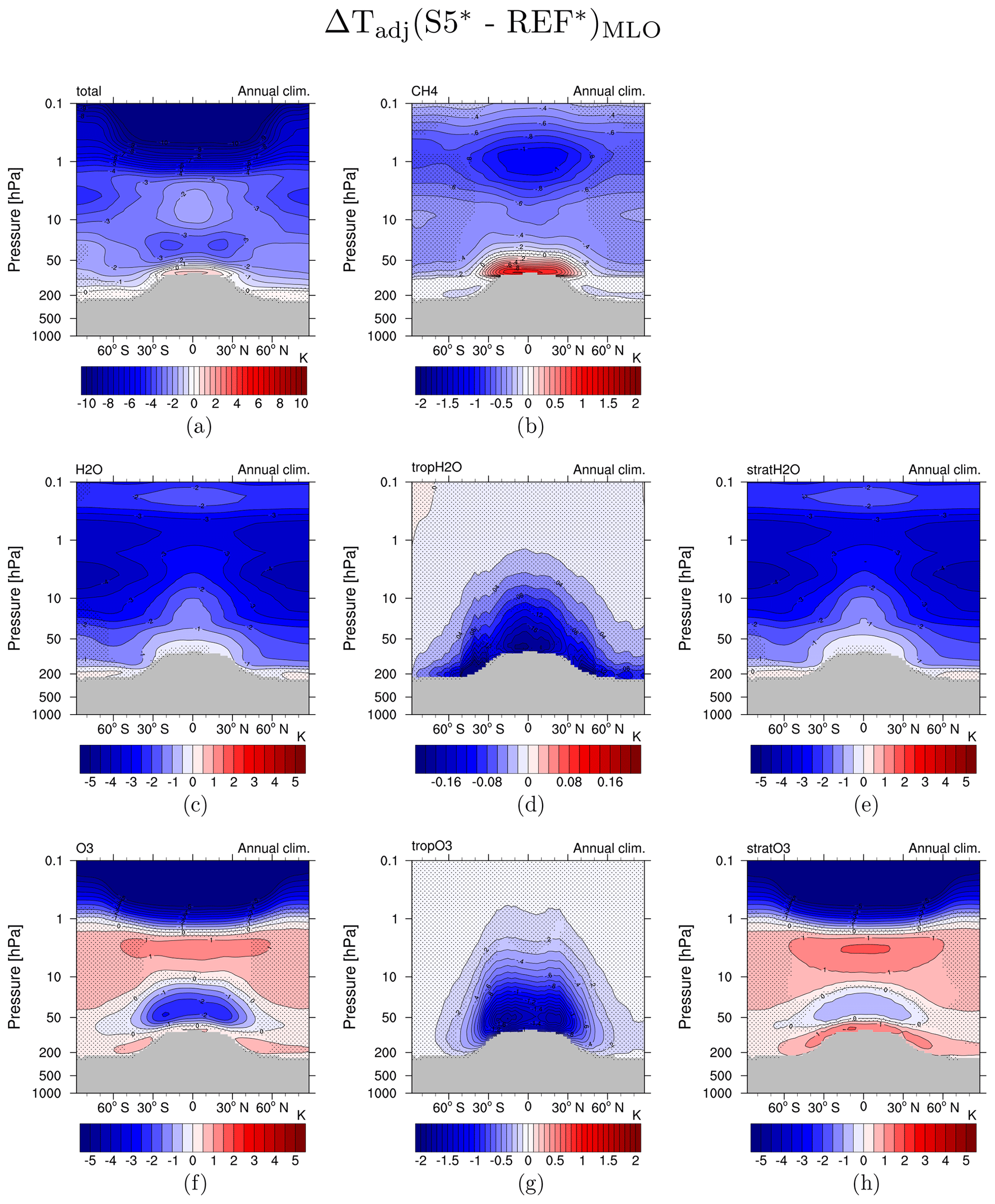
Figure 8Stratospheric temperature adjustment radiatively induced by individual species changes in simulation S5 MLO (5×CH4): (a) CH4, H2O, and O3 combined; (b) CH4; (c) H2O; (d) tropospheric H2O only; (e) stratospheric H2O only (SWV); (f) O3; (g) tropospheric O3 only; and (h) stratospheric O3 only. Note the different colour bars in (a, b, d, g).
The deep branch of the residual mean circulation is closely linked to the strength of the winter stratospheric polar vortex. An increase in the poleward flow and in downwelling at higher latitudes is accompanied with a slowdown of the stratospheric polar vortex (Kidston et al., 2015, and references therein). The S5 MLO response of zonal mean winds shows indeed an easterly change in the stratospheric polar vortex in boreal winter (DJF) (see Fig. S15). The respective response for S2 MLO is not significant but decelerating, too. The SH stratospheric polar vortex strengthens for S2 MLO but less than in S2 fSST. Nevertheless, the response of stratospheric zonal winds in both MLO experiments is substantially different from fSST in the SH as well.
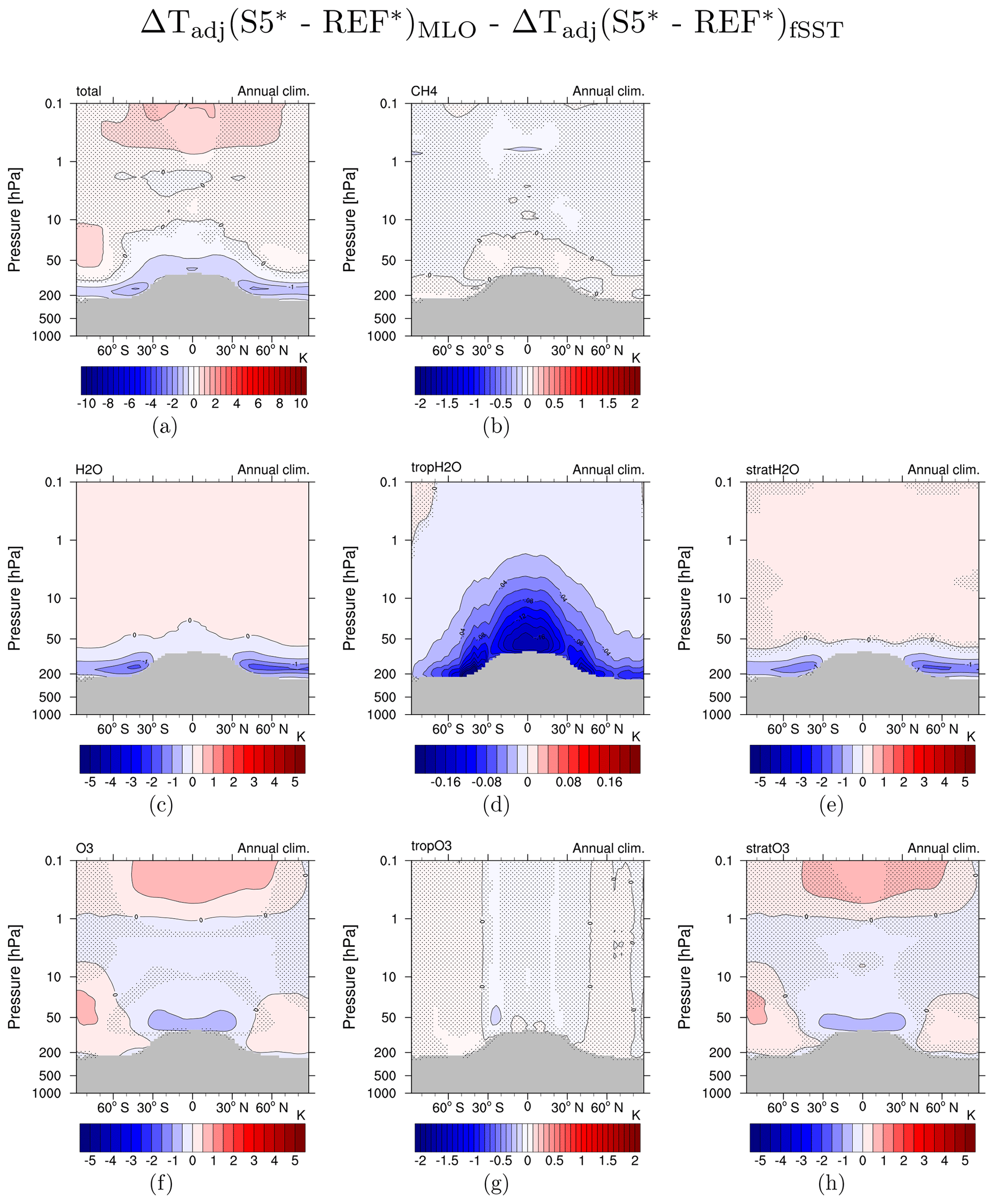
Figure 9Difference between stratospheric temperature adjustment in simulations S5 MLO and S5 fSST (5×CH4) radiatively induced by individual species changes: (a) CH4, H2O, and O3 combined; (b) CH4; (c) H2O; (d) tropospheric H2O only; (e) stratospheric H2O only (SWV); (f) O3; (g) tropospheric O3 only; and (h) stratospheric O3 only. Note the different colour bars in (a, b, d, g).
The easterly change in polar stratospheric zonal winds in the NH during DJF is consistent with the response of the stratospheric polar vortex in CMIP5 global warming simulations (Manzini et al., 2014; Karpechko and Manzini, 2017). Moreover, differences between the fSST and MLO response signals of stratospheric zonal winds during DJF are qualitatively consistent with the results of Karpechko and Manzini (2017). They identified, on the one hand, a deceleration of the stratospheric polar vortex and associated warming in the polar stratosphere in simulations driven by higher SSTs (comparable to the MLO experiments) and, on the other hand, a strengthened and cooled stratospheric polar vortex in simulations driven by CO2 increase and suppressed tropospheric warming (comparable to the fSST experiments). Karpechko and Manzini (2017) suggested that tropospheric warming and associated strengthening of subtropical winds lead to enhanced wave activity. In S5 MLO subtropical winds strengthen, indicating that similar processes might act in our simulations. However, a detailed analysis of wave activity is beyond the scope of this study.
In summary, SST-driven climate feedbacks affect the chemical composition. The differences in stratospheric temperature adjustment between MLO and fSST (see Fig. 9) reflect radiative impacts of these composition changes on stratospheric temperature. Additionally, the patterns of suggest that dynamical effects have changed significantly in the MLO simulations with respect to fSST. The dynamical temperature response effect for S5 MLO is consistent with the strengthening of the BDC. Dynamic heating counteracts the radiative cooling in the extratropical middle and upper stratosphere and in the subtropical lower stratosphere in S5 MLO. This results in reduced cooling in these regions in S5 MLO in Fig. 1d, which is not significant on annual average but in the respective winter hemispheres (not shown). for S2 MLO indicates strengthening of mainly the shallow branch of the BDC.
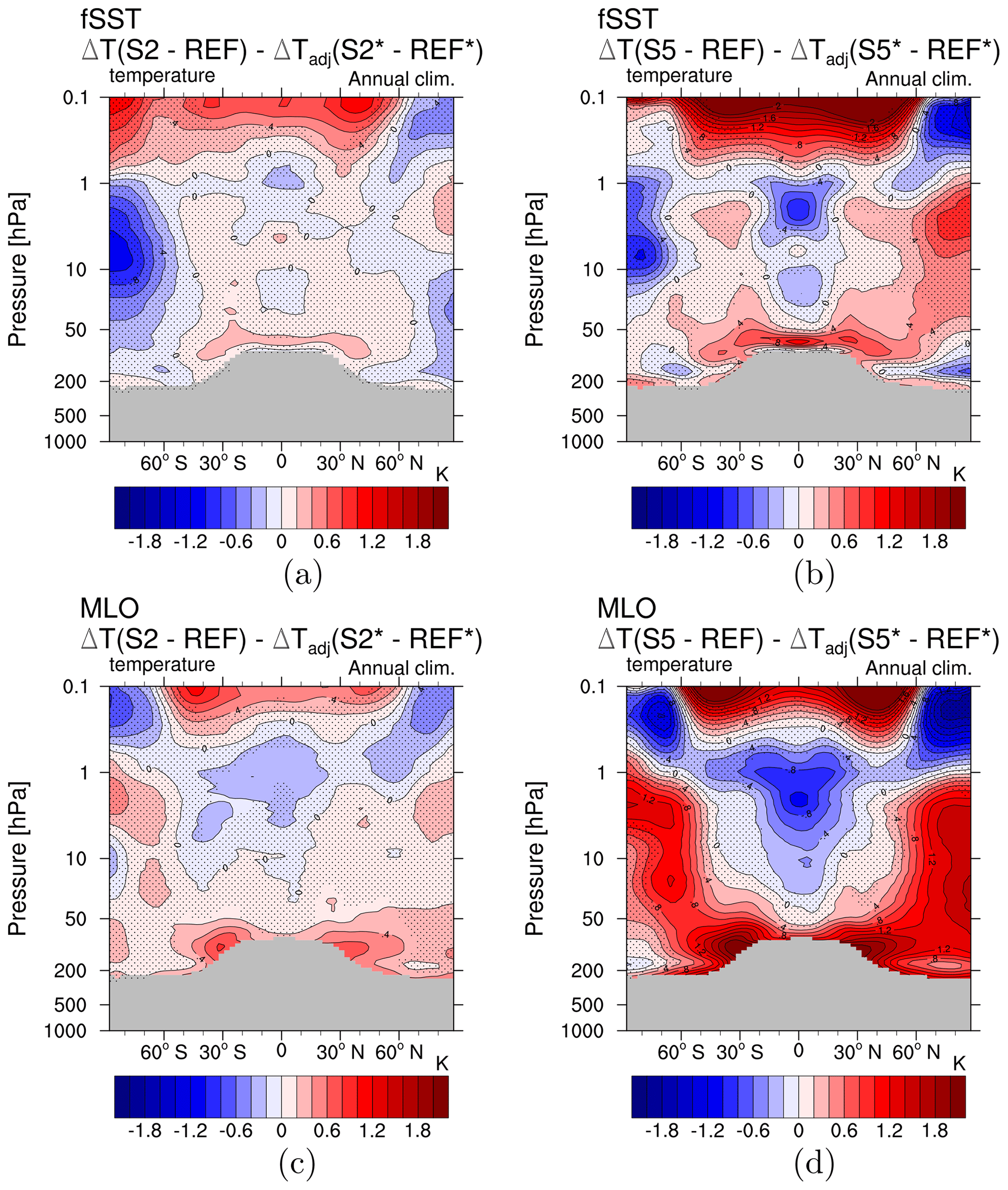
Figure 10Dynamical temperature response effect of the simulations (a) S2 fSST, (b) S5 fSST, (c) S2 MLO, (d) S5 MLO. The dynamical effect is calculated as the difference between the temperature response in the regular simulations (ΔT(SX-REF) with X either 2 or 5) and the sum of the individual contributions of CH4, H2O and O3 to the stratosphere adjusted temperatures (ΔTadj (SX∗-REF∗) with X either 2 or 5).
While it has been long-since acknowledged that the net RF of CH4 includes substantial contributions from O3 and SWV (e.g. Fig. 8.17 in IPCC, 2013, derived from Shindell et al., 2009, and Stevenson et al., 2013), it is still common to consider climate feedbacks and climate sensitivity of CH4 in comparison to CO2 without accounting for these additional radiative components (Modak et al., 2018; Smith et al., 2018; Richardson et al., 2019). Our study provides a quantification of SST-driven slow radiative feedbacks from CH4, O3, and associated SWV changes in climate sensitivity simulations forced by a twofold or fivefold CH4 increase, extending the work of Winterstein et al. (2019) on the respective rapid radiative adjustments.
The strongly enhanced CH4 mixing ratios cause enhanced depletion of OH in the troposphere. Tropospheric warming, in contrast, results in enhanced OH precursors and causes the reduction in OH in the troposphere to be weaker than in the prescribed SST simulations analysed by Winterstein et al. (2019). Additionally, the acceleration of the CH4 oxidation at higher temperatures leads to a more efficient depletion of CH4 in a warming troposphere. This so-called climate offset results in a reduced prolongation of the tropospheric CH4 lifetime and is consistent with previous CCM studies (Voulgarakis et al., 2013). The prolonged tropospheric CH4 lifetime has the effect that the corresponding CH4 surface fluxes increase by a smaller factor than the mixing ratio.
Changes in the stratospheric circulation can be clearly identified in the sensitivity simulations that include SST-driven climate feedbacks on top of the quasi-instantaneous response analysed by Winterstein et al. (2019). Tropospheric warming leads to the acceleration of the BDC in our sensitivity simulations as expected from climate change scenario calculations (Butchart, 2014). In the lower tropical stratosphere, both the decrease in O3 and the associated cooling as well as the increase in CH4 become more distinct, which reflects the more pronounced acceleration of tropical upwelling induced by a warming troposphere. The strengthening of the BDC also manifests in the temperature response. Whereas the stratospheric polar vortices in both winter hemispheres strengthen in the experiments with prescribed SSTs and SICs, polar stratospheric zonal winds decelerate in northern winter in the sensitivity simulations that include tropospheric warming consistent with the response in CMIP5 global warming simulations (Manzini et al., 2014; Karpechko and Manzini, 2017).
As a result of tropical upper troposphere moistening, increased tropical upwelling, and more pronounced warming of the cold point, the transport of tropospheric H2O into the lower stratosphere is more strongly enhanced in the sensitivity simulations that include SST-driven climate feedbacks, resulting in a stronger increase in SWV in the lower extratropical stratosphere. In the middle and upper stratosphere, where CH4 oxidation makes an important contribution to SWV, the increase in SWV is weakened in the present sensitivity simulations compared to the quasi-instantaneous response. Less pronounced increases in stratospheric OH in response to the slow adjustments in comparison to the quasi-instantaneous response cause the depletion of CH4 to be weaker and thus reduce the in situ source of SWV as well.
The contribution of SST-driven climate feedbacks to the total CH4-induced O3 response shows remarkable similarities to the O3 response to climate feedbacks in CO2-forced climate change simulations (Dietmüller et al., 2014; Nowack et al., 2018; Chiodo and Polvani, 2019). The consistency between the O3 feedbacks resulting from these different forcing agents encourages the separation of the O3 response patterns into rapid adjustments and climate feedbacks in future studies. Rapid adjustments are specific to the forcing, whereas climate feedbacks are driven by surface temperature changes and are therefore expected to be less dependent on the forcing agent (Sherwood et al., 2015). However, the overall response of O3 (rapid adjustments and slow feedbacks) is quite different under CH4 forcing compared to CO2 forcing owing to chemically induced feedbacks under CH4 forcing. Chiodo and Polvani (2017) and Nowack et al. (2017) suggested that feedbacks from interactive O3 under CO2 forcing have the potential to significantly alter the tropospheric circulation. As the overall O3 response is different under CH4 forcing, also modified feedbacks on the tropospheric circulation are expected. Those are planned to be assessed using a simulation set-up with a CH4 emission flux boundary condition to simulate feedbacks of tropospheric CH4 to changes in its chemical sinks.
The doubled and quintupled CH4 mixing ratios result in global mean surface temperature changes of 0.42 ± 0.05 K and 1.28 ± 0.04 K, respectively. We estimate the corresponding climate sensitivity parameters λ using these temperature changes and the respective RIs from CH4 with the respective chemical adjustments included, as determined by Winterstein et al. (2019), which can well be interpreted as the corresponding ERFs. The respective estimate of λ for 5×CH4 compares well with an estimate from CO2-driven climate change simulations with EMAC with a comparable magnitude of RI (Rieger et al., 2017), suggesting an efficacy of CH4 ERF close to unity. The estimate of λ corresponding to 2×CH4 is smaller than the respective value for 5×CH4 but has a large uncertainty. Considering the large uncertainty and inter-model spread (Richardson et al., 2019) of this parameter, we conclude that a more targeted experimental design is necessary to exactly quantify the effect of chemical feedbacks on the climate sensitivity in CH4-driven scenarios and on the associated CH4 efficacy.
The RIs from the purely SST-driven response of CH4 and O3 are small. The RIs resulting from changes in tropospheric and stratospheric H2O are enlarged by SST-driven climate feedbacks. Increased tropospheric humidity in a warming troposphere enhances the RI. The reason for the enlarged RI from SWV is its more pronounced increase in the lower stratosphere, where its changes dominate the induced RI (Solomon et al., 2010). As the increase in SWV in this region is likely induced by transport from the warmer tropical troposphere, this part of the RI increase cannot be regarded to be chemically induced. The associated responses of stratosphere adjusted temperatures from the purely SST-driven response are dominated by the changes in SWV just explained and by decreases in stratospheric O3 in the lowermost tropical stratosphere. It is worth noting that tropospheric CH4 mixing ratios do not respond to changes in tropospheric sinks (e.g. OH) in the used simulation set-up as its mixing ratio is prescribed at the lower boundary. The prolongation of the tropospheric CH4 lifetime indicates a positive feedback on the CH4 mixing ratio and thus on the induced RI. In a future study, climate change scenario simulations conducted with a CCM with realistic CH4 emission fluxes are planned to quantify this chemical feedback of CH4.
In the present study we are able for the first time to quantify the effects of slow climate feedbacks on the chemical composition and circulation in CH4-forced climate change scenarios and further evaluate them in comparison to the quasi-instantaneous atmospheric response.
The MLO simulations were carried out with a more recent MESSy version with regard to the fSST simulations (2.54.0 instead of 2.52). This involves changes to the chemistry module MECCA (Sander et al., 2011) including the update of reaction rate coefficients to the latest recommendations, Evaluation No. 18 of the Jet Propulsion Laboratory (Burkholder et al., 2015), and to values coming from other recent laboratory studies. A table of all affected reactions can be found in the Supplement (Table S1). Moreover, the yield of the photolysis of CFCl3 (CFC-11) and CF2Cl2 (CFC-12) changed from three and two, respectively, to one chlorine (Cl) atom. The smaller Cl yield influences the O3 mixing ratio in the stratosphere as Cl acts as a catalyst in the O3-depleting cycles. The O3 mixing ratio is higher everywhere in the stratosphere, except in the lowermost tropical stratosphere, in REF MLO compared to REF fSST (see Fig. S17). This results further in higher temperatures in the stratosphere in REF MLO (not shown). The contribution of the ClOx O3-depleting cycle to total O3 loss peaks at around 40 to 45 km altitude (see Fig. 5.28 in Seinfeld and Pandis, 2016). This corresponds approximately to the altitude of the maximum relative difference in O3 mixing ratio between REF MLO and REF fSST (see Fig. S17).
In the REF QFLX simulation the setting of the non-orographic gravity wave drag parameterization (GWAVE; Baumgaertner et al., 2013) was different than in all the other simulations (fSST and MLO), in which breaking of gravity waves transfers only momentum but no heat. In REF QFLX heat is also transferred, leading to higher temperatures in the mesosphere. Since predominantly the mesosphere is affected, the different setting does not considerably influence the retrieved heat flux correction at the surface, the determination of which is the purpose of REF QFLX.
The Modular Earth Submodel System (MESSy) is continuously developed and applied by a consortium of institutions. The usage of MESSy and access to the source code are licensed to all affiliates of institutions that are members of the MESSy Consortium. Institutions can become members of the MESSy Consortium by signing the MESSy Memorandum of Understanding. More information can be found on the MESSy Consortium website (https://www.messy-interface.org/, last access: 27 May 2020; Jöckel and the MESSy Consortium, 2020). Furthermore the exact code version used to produce the simulation results is archived at the German Climate Computing Center (DKRZ) and can be made available to members of the MESSy community upon request. The simulation results are also archived at DKRZ and are available upon request.
The supplement related to this article is available online at: https://doi.org/10.5194/acp-21-731-2021-supplement.
The simulations were set up and carried out by PJ and FW with contributions of MK in applying the MLOCEAN submodel. MP and FW conceived and carried out the radiative impact and stratosphere adjusted temperature calculations, and FW created the corresponding figures. LS analysed the data, created the remaining figures, and prepared the manuscript with significant contributions regarding the interpretation and evaluation of the model results from all coauthors.
The authors declare that they have no conflict of interest.
This article is part of the special issue “The Modular Earth Submodel System (MESSy) (ACP/GMD inter-journal SI)”. It is not associated with a conference.
We acknowledge the financial support by the DLR internal projects KliSAW (Klimarelevanz von atmosphärischen Spurengasen, Aerosolen und Wolken) and MABAK (Innovative Methoden zur Analyse und Bewertung von Veränderungen der Atmosphäre und des Klimasystems). The model simulations have been performed at the German Climate Computing Centre (DKRZ) through support from the Bundesministerium für Bildung und Forschung (BMBF). We used the Climate Data Operators (CDO; https://code.mpimet.mpg.de/projects/cdo, last access: 9 December 2020) for data processing and the NCAR Command Language (NCL; https://doi.org/10.5065/D6WD3XH5, last access: 9 December 2020) for data analysis and to create the figures of this study. We furthermore thank all contributors of the project ESCiMo (Earth System Chemistry integrated Modelling), which provided the model configuration and initial conditions. We thank Roland Eichinger for his constructive internal review of the manuscript and Hella Garny for her helpful comments on the interpretation of the dynamically induced temperature response. Finally, we thank Holger Tost for editing this paper and Peer Johannes Nowack and one anonymous reviewer for their comments that improved the manuscript.
This research has been supported by the DFG (Deutsche Forschungsgemeinschaft) (grant no. WI 5369/1-1).
This paper was edited by Holger Tost and reviewed by Peer Johannes Nowack and one anonymous referee.
Austin, J., Wilson, J., Li, F., and Vömel, H.: Evolution of Water Vapor Concentrations and Stratospheric Age of Air in Coupled Chemistry – Climate Model Simulations, J. Atmos. Sci., 64, 905–921, https://doi.org/10.1175/JAS3866.1, 2007. a, b
Baumgaertner, A. J. G., Jöckel, P., Aylward, A. D., and Harris, M. J.: Simulation of Particle Precipitation Effects on the Atmosphere with the MESSy Model System, in: Climate and Weather of the Sun-Earth System (CAWSES), edited by: Lübken, F.-J., Springer, Dordrecht, Netherlands, 301–316, https://doi.org/10.1007/978-94-007-4348-9_17, 2013. a
Birner, T. and Bönisch, H.: Residual circulation trajectories and transit times into the extratropical lowermost stratosphere, Atmos. Chem. Phys., 11, 817–827, https://doi.org/10.5194/acp-11-817-2011, 2011. a
Bony, S., Bellon, G., Klocke, D., Sherwood, S., Fermepin, S., and Denvil, S.: Robust direct effect of carbon dioxide on tropical circulation and regional precipitation, Nat. Geosci., 6, 447–451, https://doi.org/10.1038/ngeo1799, 2013. a
Burkholder, J. B., Sander, S. P., Abbatt, J. P. D., Barker, J. R., Huie, R. E., Kolb, C. E., Kurylo, M. J., Orkin, V. L., Wilmouth, D. M., and Wine, P. H.: Chemical Kinetics and Photochemical Data for Use in Atmospheric Studies, Evaluation No. 18, JPL Publication 15–10, Jet Propulsion Laboratory, http://jpldataeval.jpl.nasa.gov/, 2015. a
Butchart, N.: The Brewer-Dobson circulation, Rev. Geophys., 52, 157–184, https://doi.org/10.1002/2013RG000448, 2014. a, b, c, d
Butchart, N. and Scaife, A. A.: Removal of chlorofluorocarbons by increased mass exchange between the stratosphere and troposphere in a changing climate, Nature, 410, 799–802, https://doi.org/10.1038/35071047, 2001. a
Chiodo, G. and Polvani, L. M.: Reduced Southern Hemispheric circulation response to quadrupled CO2 due to stratospheric ozone feedback, Geophys. Res. Lett., 44, 465–474, https://doi.org/10.1002/2016GL071011, 2017. a
Chiodo, G. and Polvani, L. M.: The Response of the Ozone Layer to Quadrupled CO2 Concentrations: Implications for Climate, J. Climate, 32, 7629–7642, https://doi.org/10.1175/JCLI-D-19-0086.1, 2019. a, b
Colman, R. A. and McAvaney, B. J.: On tropospheric adjustment to forcing and climate feedbacks, Clim. Dynam., 36, 1649–1658, https://doi.org/10.1007/s00382-011-1067-4, 2011. a
Danabasoglu, G. and Gent, P. R.: Equilibrium climate sensitivity: Is it accurate to use a slab ocean model?, J. Climate, 22, 2494–2499, https://doi.org/10.1175/2008JCLI2596.1, 2009. a
Dean, J. F., Middelburg, J. J., Röckmann, T., Aerts, R., Blauw, L. G., Egger, M., Jetten, M. S. M., de Jong, A. E. E., Meisel, O. H., Rasigraf, O., Slomp, C. P., in't Zandt, M. H., and Dolman, A. J.: Methane Feedbacks to the Global Climate System in a Warmer World, Rev. Geophys., 56, 207–250, https://doi.org/10.1002/2017RG000559, 2018. a
Dietmüller, S., Ponater, M., and Sausen, R.: Interactive ozone induces a negative feedback in CO2-driven climate change simulations, J. Geophys. Res.-Atmos., 119, 1796–1805, https://doi.org/10.1002/2013JD020575, 2014. a, b, c
Dietmüller, S., Jöckel, P., Tost, H., Kunze, M., Gellhorn, C., Brinkop, S., Frömming, C., Ponater, M., Steil, B., Lauer, A., and Hendricks, J.: A new radiation infrastructure for the Modular Earth Submodel System (MESSy, based on version 2.51), Geosci. Model Dev., 9, 2209–2222, https://doi.org/10.5194/gmd-9-2209-2016, 2016. a, b, c, d
Dietmüller, S., Eichinger, R., Garny, H., Birner, T., Boenisch, H., Pitari, G., Mancini, E., Visioni, D., Stenke, A., Revell, L., Rozanov, E., Plummer, D. A., Scinocca, J., Jöckel, P., Oman, L., Deushi, M., Kiyotaka, S., Kinnison, D. E., Garcia, R., Morgenstern, O., Zeng, G., Stone, K. A., and Schofield, R.: Quantifying the effect of mixing on the mean age of air in CCMVal-2 and CCMI-1 models, Atmos. Chem. Phys., 18, 6699–6720, https://doi.org/10.5194/acp-18-6699-2018, 2018. a
Dunne, J. P., Winton, M., Bacmeister, J., Danabasoglu, G., Gettelman, A., Golaz, J.-C., Hannay, C., Schmidt, G. A., Krasting, J. P., Leung, L. R., Nazarenko, L., Sentman, L. T., Stouffer, R. J., and Wolfe, J. D.: Comparison of Equilibrium Climate Sensitivity Estimates From Slab Ocean, 150-Year, and Longer Simulations, Geophys. Res. Lett., 47, e2020GL088852, https://doi.org/10.1029/2020GL088852, 2020. a
Eichinger, R., Dietmüller, S., Garny, H., Šácha, P., Birner, T., Bönisch, H., Pitari, G., Visioni, D., Stenke, A., Rozanov, E., Revell, L., Plummer, D. A., Jöckel, P., Oman, L., Deushi, M., Kinnison, D. E., Garcia, R., Morgenstern, O., Zeng, G., Stone, K. A., and Schofield, R.: The influence of mixing on the stratospheric age of air changes in the 21st century, Atmos. Chem. Phys., 19, 921–940, https://doi.org/10.5194/acp-19-921-2019, 2019. a, b, c
Forster, P. M., Richardson, T., Maycock, A. C., Smith, C. J., Samset, B. H., Myhre, G., Andrews, T., Pincus, R., and Schulz, M.: Recommendations for diagnosing effective radiative forcing from climate models for CMIP6, J. Geophys. Res.-Atmos., 121, 12460–12475, https://doi.org/10.1002/2016JD025320, 2016. a
Frank, F., Jöckel, P., Gromov, S., and Dameris, M.: Investigating the yield of H2O and H2 from methane oxidation in the stratosphere, Atmos. Chem. Phys., 18, 9955–9973, https://doi.org/10.5194/acp-18-9955-2018, 2018. a, b
Garcia, R. R. and Randel, W. J.: Acceleration of the Brewer-Dobson Circulation due to Increases in Greenhouse Gases, J. Atmos. Sci., 65, 2731–2739, https://doi.org/10.1175/2008JAS2712.1, 2008. a
Geoffroy, O., Saint-Martin, D., Voldoire, A., Salasy Melia, D., and Senesi, S.: Adjusted radiative forcing and global radiative feedbacks in CNRM-CM5, a closure of the partial decomposition, Clim. Dynam., 42, 1807–1818, https://doi.org/10.1007/s00382-013-1741-9, 2014. a
Gregory, J. M., Ingram, W. J., Palmer, M. A., Jones, G. S., Stott, P. A., Thorpe, R. B., Lowe, J. A., Johns, T. C., and Williams, K. D.: A new method for diagnosing radiative forcing and climate sensitivity, Geophys. Res. Lett., 31, L03205, https://doi.org/10.1029/2003GL018747, 2004. a
Hansen, J., Sato, M., Ruedy, R., Nazarenko, L., Lacis, A., Schmidt, G. A., Russell, G., Aleinov, I., Bauer, M., Bauer, S., Bell, N., Cairns, B., Canuto, V., Chandler, M., Cheng, Y., Del Genio, A., Faluvegi, G., Fleming, E., Friend, A., Hall, T., Jackman, C., Kelley, M., Kiang, N., Koch, D., Lean, J., Lerner, J., Lo, K., Menon, S., Miller, R., Minnis, P., Novakov, T., Oinas, V., Perlwitz, J., Perlwitz, J., Rind, D., Romanou, A., Shindell, D., Stone, P., Sun, S., Tausnev, N., Thresher, D., Wielicki, B., Wong, T., Yao, M., and Zhang, S.: Efficacy of climate forcings, J. Geophys. Res.-Atmos, 110, D18104, https://doi.org/10.1029/2005JD005776, 2005. a, b
Hein, R., Dameris, M., Schnadt, C., Land, C., Grewe, V., Köhler, I., Ponater, M., Sausen, R., B. Steil, B., Landgraf, J., and Brühl, C.: Results of an interactively coupled atmospheric chemistry – general circulation model: Comparison with observations, Ann. Geophys., 19, 435–457, https://doi.org/10.5194/angeo-19-435-2001, 2001. a
IPCC: Climate Change 2013: The Physical Science Basis. Contribution of Working Group I to the Fifth Assessment Report of the Intergovernmental Panel on Climate Change, edited by: Stocker, T. F., Qin, D., Plattner, G.-K., Tignor, M., Allen, S. K., Boschung, J., Nauels, A., Xia, Y., Bex, V., and Midgley, P. M., Cambridge University Press, Cambridge, United Kingdom and New York, USA, https://doi.org/10.1017/CBO9781107415324, 2013. a, b, c, d
Jöckel, P., Tost, H., Pozzer, A., Brühl, C., Buchholz, J., Ganzeveld, L., Hoor, P., Kerkweg, A., Lawrence, M. G., Sander, R., Steil, B., Stiller, G., Tanarhte, M., Taraborrelli, D., van Aardenne, J., and Lelieveld, J.: The atmospheric chemistry general circulation model ECHAM5/MESSy1: consistent simulation of ozone from the surface to the mesosphere, Atmos. Chem. Phys., 6, 5067–5104, https://doi.org/10.5194/acp-6-5067-2006, 2006. a
Jöckel, P., Tost, H., Pozzer, A., Kunze, M., Kirner, O., Brenninkmeijer, C. A. M., Brinkop, S., Cai, D. S., Dyroff, C., Eckstein, J., Frank, F., Garny, H., Gottschaldt, K.-D., Graf, P., Grewe, V., Kerkweg, A., Kern, B., Matthes, S., Mertens, M., Meul, S., Neumaier, M., Nützel, M., Oberländer-Hayn, S., Ruhnke, R., Runde, T., Sander, R., Scharffe, D., and Zahn, A.: Earth System Chemistry integrated Modelling (ESCiMo) with the Modular Earth Submodel System (MESSy) version 2.51, Geosci. Model Dev., 9, 1153–1200, https://doi.org/10.5194/gmd-9-1153-2016, 2016. a, b, c, d
Jöckel, P. and the MESSy Consortium: The highly structured Modular Earth Submodel System (MESSy), availabe at: http://www.messy-interface.org, last access: 27 May 2020. a
Karpechko, A. Y. and Manzini, E.: Arctic Stratosphere Dynamical Response to Global Warming, J. Climate, 30, 7071–7086, https://doi.org/10.1175/JCLI-D-16-0781.1, 2017. a, b, c, d
Kerkweg, A., Sander, R., Tost, H., and Jöckel, P.: Technical note: Implementation of prescribed (OFFLEM), calculated (ONLEM), and pseudo-emissions (TNUDGE) of chemical species in the Modular Earth Submodel System (MESSy), Atmos. Chem. Phys., 6, 3603–3609, https://doi.org/10.5194/acp-6-3603-2006, 2006. a
Kidston, J., Scaife, A. A., Hardiman, S. C., Mitchell, D. M., Butchart, N., Baldwin, M. P., and Gray, L. J.: Stratospheric influence on tropospheric jet streams, storm tracks and surface weather, Nat. Geosci., 8, 433–440, https://doi.org/10.1038/ngeo2424, 2015. a
Kirner, O., Ruhnke, R., and Sinnhuber, B.-M.: Chemistry – Climate Interactions of Stratospheric and Mesospheric Ozone in EMAC Long-Term Simulations with Different Boundary Conditions for CO2, CH4, N2O, and ODS, Atmos. Ocean, 53, 140–152, https://doi.org/10.1080/07055900.2014.980718, 2015. a, b
Klappenbach, F., Bertleff, M., Kostinek, J., Hase, F., Blumenstock, T., Agusti-Panareda, A., Razinger, M., and Butz, A.: Accurate mobile remote sensing of XCO2 and XCH4 latitudinal transects from aboard a research vessel, Atmos. Meas. Tech., 8, 5023–5038, https://doi.org/10.5194/amt-8-5023-2015, 2015. a, b
Kunze, M., Godolt, M., Langematz, U., Grenfell, J., Hamann-Reinus, A., and Rauer, H.: Investigating the early Earth faint young Sun problem with a general circulation model, Planet. Space Sci., 98, 77–92, https://doi.org/10.1016/j.pss.2013.09.011, 2014. a
Lawrence, M. G., Jöckel, P., and von Kuhlmann, R.: What does the global mean OH concentration tell us?, Atmos. Chem. Phys., 1, 37–49, https://doi.org/10.5194/acp-1-37-2001, 2001. a
Li, C., von Storch, J.-S., and Marotzke, J.: Deep-ocean heat uptake and equilibrium climate response, Clim. Dynam., 40, 1071–1086, https://doi.org/10.1007/s00382-012-1350-z, 2013. a
Lin, P., Paynter, D., Ming, Y., and Ramaswamy, V.: Changes of the Tropical Tropopause Layer under Global Warming, J. Climate, 30, 1245–1258, https://doi.org/10.1175/JCLI-D-16-0457.1, 2017. a
Manzini, E., Karpechko, A. Y., Anstey, J., Baldwin, M. P., Black, R. X., Cagnazzo, C., Calvo, N., Charlton-Perez, A., Christiansen, B., Davini, P., Gerber, E., Giorgetta, M., Gray, L., Hardiman, S. C., Lee, Y.-Y., Marsh, D. R., McDaniel, B. A., Purich, A., Scaife, A. A., Shindell, D., Son, S.-W., Watanabe, S., and Zappa, G.: Northern winter climate change: Assessment of uncertainty in CMIP5 projections related to stratosphere-troposphere coupling, J. Geophys. Res.-Atmos., 119, 7979–7998, https://doi.org/10.1002/2013JD021403, 2014. a, b
Modak, A., Bala, G., Caldeira, K., and Cao, L.: Does shortwave absorption by methane influence its effectiveness?, Clim. Dynam., 51, 3653–3672, https://doi.org/10.1007/s00382-018-4102-x, 2018. a, b, c, d
Morgenstern, O., Stone, K. A., Schofield, R., Akiyoshi, H., Yamashita, Y., Kinnison, D. E., Garcia, R. R., Sudo, K., Plummer, D. A., Scinocca, J., Oman, L. D., Manyin, M. E., Zeng, G., Rozanov, E., Stenke, A., Revell, L. E., Pitari, G., Mancini, E., Di Genova, G., Visioni, D., Dhomse, S. S., and Chipperfield, M. P.: Ozone sensitivity to varying greenhouse gases and ozone-depleting substances in CCMI-1 simulations, Atmos. Chem. Phys., 18, 1091–1114, https://doi.org/10.5194/acp-18-1091-2018, 2018. a
Nisbet, E. G., Manning, M. R., Dlugokencky, E. J., Fisher, R. E., Lowry, D., Michel, S. E., Myhre, C. L., Platt, S. M., Allen, G., Bousquet, P., Brownlow, R., Cain, M., France, J. L., Hermansen, O., Hossaini, R., Jones, A. E., Levin, I., Manning, A. C., Myhre, G., Pyle, J. A., Vaughn, B. H., Warwick, N. J., and White, J. W. C.: Very Strong Atmospheric Methane Growth in the 4 Years 2014–2017: Implications for the Paris Agreement, Global Biogeochem. Cy., 33, 318–342, https://doi.org/10.1029/2018GB006009, https://agupubs.onlinelibrary.wiley.com/doi/abs/10.1029/2018GB006009, 2019. a
Nowack, P. J., Braesicke, P., Luke Abraham, N., and Pyle, J. A.: On the role of ozone feedback in the ENSO amplitude response under global warming, Geophys. Res. Lett., 44, 3858–3866, https://doi.org/10.1002/2016GL072418, 2017. a
Nowack, P. J., Abraham, N. L., Braesicke, P., and Pyle, J. A.: The Impact of Stratospheric Ozone Feedbacks on Climate Sensitivity Estimates, J. Geophys. Res.-Atmos., 123, 4630–4641, https://doi.org/10.1002/2017JD027943, 2018. a, b
Plumb, R. A.: Stratospheric Transport, J. Meteorol. Soc. Jpn. Ser. II, 80, 793–809, https://doi.org/10.2151/jmsj.80.793, 2002. a
Randel, W. and Park, M.: Diagnosing Observed Stratospheric Water Vapor Relationships to the Cold Point Tropical Tropopause, J. Geophys. Res.-Atmos., 124, 7018–7033, https://doi.org/10.1029/2019JD030648, 2019. a
Rayner, N. A., Parker, D. E., Horton, E. B., Folland, C. K., Alexander, L. V., Rowell, D. P., Kent, E. C., and Kaplan, A.: Global analyses of sea surface temperature, sea ice, and night marine air temperature since the late nineteenth century, J. Geophys. Res.-Atmos., 108, 4407, https://doi.org/10.1029/2002JD002670, 2003. a, b, c
Revell, L. E., Stenke, A., Rozanov, E., Ball, W., Lossow, S., and Peter, T.: The role of methane in projections of 21st century stratospheric water vapour, Atmos. Chem. Phys., 16, 13067–13080, https://doi.org/10.5194/acp-16-13067-2016, 2016. a, b, c
Richardson, T. B., Forster, P. M., Smith, C. J., Maycock, A. C., Wood, T., Andrews, T., Boucher, O., Faluvegi, G., Fläschner, D., Hodnebrog, Ø., Kasoar, M., Kirkevåg, A., Lamarque, J.-F., Mülmenstädt, J., Myhre, G., Olivié, D., Portmann, R. W., Samset, B. H., Shawki, D., Shindell, D., Stier, P., Takemura, T., Voulgarakis, A., and Watson-Parris, D.: Efficacy of Climate Forcings in PDRMIP Models, J. Geophys. Res.-Atmos., 124, 12824–12844, https://doi.org/10.1029/2019JD030581, 2019. a, b, c, d, e, f, g
Rieger, V. S., Dietmüller, S., and Ponater, M.: Can feedback analysis be used to uncover the physical origin of climate sensitivity and efficacy differences?, Clim. Dynam., 49, 2831–2844, https://doi.org/10.1007/s00382-016-3476-x, 2017. a, b, c
Rind, D., Suozzo, R., Balachandran, N. K., and Prather, M. J.: Climate Change and the Middle Atmosphere Part I: The Doubled CO2 Climate, J. Atmos. Sci., 47, 475–494, 1990. a
Röckmann, T., Brass, M., Borchers, R., and Engel, A.: The isotopic composition of methane in the stratosphere: high-altitude balloon sample measurements, Atmos. Chem. Phys., 11, 13287–13304, https://doi.org/10.5194/acp-11-13287-2011, 2011. a
Roeckner, E., Siebert, T., and Feichter, J.: Climatic response to anthropogenic sulfate forcing simulated with a general circulation model, Aerosol forcing of climate, edited by: Charlson, R. J., Heinzenberg, J., John Wiley and Sons, Chichester, 349–362, 1995. a
Rohs, S., Schiller, C., Riese, M., Engel, A., Schmidt, U., Wetter, T., Levin, I., Nakazawa, T., and Aoki, S.: Long-term changes of methane and hydrogen in the stratosphere in the period 1978–2003 and their impact on the abundance of stratospheric water vapor, J. Geophys. Res.-Atmos., 111, 1–12, https://doi.org/10.1029/2005JD006877, 2006. a
Rosier, S. M. and Shine, K. P.: The effect of two decades of ozone change on stratospheric temperature as indicated by a general circulation model, Geophys. Res. Lett., 27, 2617–2620, https://doi.org/10.1029/2000GL011584, 2000. a
Sander, R., Baumgaertner, A., Gromov, S., Harder, H., Jöckel, P., Kerkweg, A., Kubistin, D., Regelin, E., Riede, H., Sandu, A., Taraborrelli, D., Tost, H., and Xie, Z.-Q.: The atmospheric chemistry box model CAABA/MECCA-3.0, Geosci. Model Dev., 4, 373–380, https://doi.org/10.5194/gmd-4-373-2011, 2011. a, b
Saunois, M., Bousquet, P., Poulter, B., Peregon, A., Ciais, P., Canadell, J. G., Dlugokencky, E. J., Etiope, G., Bastviken, D., Houweling, S., Janssens-Maenhout, G., Tubiello, F. N., Castaldi, S., Jackson, R. B., Alexe, M., Arora, V. K., Beerling, D. J., Bergamaschi, P., Blake, D. R., Brailsford, G., Brovkin, V., Bruhwiler, L., Crevoisier, C., Crill, P., Covey, K., Curry, C., Frankenberg, C., Gedney, N., Höglund-Isaksson, L., Ishizawa, M., Ito, A., Joos, F., Kim, H.-S., Kleinen, T., Krummel, P., Lamarque, J.-F., Langenfelds, R., Locatelli, R., Machida, T., Maksyutov, S., McDonald, K. C., Marshall, J., Melton, J. R., Morino, I., Naik, V., O'Doherty, S., Parmentier, F.-J. W., Patra, P. K., Peng, C., Peng, S., Peters, G. P., Pison, I., Prigent, C., Prinn, R., Ramonet, M., Riley, W. J., Saito, M., Santini, M., Schroeder, R., Simpson, I. J., Spahni, R., Steele, P., Takizawa, A., Thornton, B. F., Tian, H., Tohjima, Y., Viovy, N., Voulgarakis, A., van Weele, M., van der Werf, G. R., Weiss, R., Wiedinmyer, C., Wilton, D. J., Wiltshire, A., Worthy, D., Wunch, D., Xu, X., Yoshida, Y., Zhang, B., Zhang, Z., and Zhu, Q.: The global methane budget 2000–2012, Earth Syst. Sci. Data, 8, 697–751, https://doi.org/10.5194/essd-8-697-2016, 2016a. a
Saunois, M., Jackson, R. B., Bousquet, P., Poulter, B., and Canadell, J. G.: The growing role of methane in anthropogenic climate change, Environ. Res. Lett., 11, 120207, https://doi.org/10.1088/1748-9326/11/12/120207, 2016b. a
Schnadt, C., Dameris, M., Ponater, M., Hein, R., Grewe, V., and Steil, B.: Interaction of atmospheric chemistry and climate and its impact on stratospheric ozone, Clim. Dynam., 18, 501–517, https://doi.org/10.1007/s00382-001-0190-z, 2002. a
Seinfeld, J. H. and Pandis, S. N.: Atmospheric Chemistry and Physics: From Air Pollution to Climate Change, John Wiley and Sons, Chichester, 2016. a
Sherwood, S. C., Bony, S., Boucher, O., Bretherton, C., Forster, P. M., Gregory, J. M., and Stevens, B.: Adjustments in the Forcing-Feedback Framework for Understanding Climate Change, B. Am. Meteorol. Soc., 96, 217–228, https://doi.org/10.1175/BAMS-D-13-00167.1, 2015. a, b
Shindell, D. T., Faluvegi, G., Bell, N., and Schmidt, G. A.: An emissions-based view of climate forcing by methane and tropospheric ozone, Geophys. Res. Lett., 32, 1–4, https://doi.org/10.1029/2004GL021900, 2005. a
Shindell, D. T., Faluvegi, G., Koch, D. M., Schmidt, G. A., Unger, N., and Bauer, S. E.: Improved Attribution of Climate Forcing to Emissions, Science, 326, 716–718, https://doi.org/10.1126/science.1174760, 2009. a, b, c
Shine, K. P., Cook, J., Highwood, E. J., and Joshi, M. M.: An alternative to radiative forcing for estimating the relative importance of climate change mechanisms, Geophys. Res. Lett., 30, 2047, https://doi.org/10.1029/2003GL018141, 2003. a
Smith, C. J., Kramer, R. J., Myhre, G., Forster, P. M., Soden, B., Andrews, T., Boucher, O., Faluvegi, G., Fläschner, D., Hodnebrog, Ø., Kasoar, M., Kharin, V., Kirkevåg, A., Lamarque, J.-F., Mülmenstädt, J., Olivié, D., Richardson, T., Samset, B. H., Shindell, D., Stier, P., Takemura, T., Voulgarakis, A., and Watson-Parris, D.: Understanding Rapid Adjustments to Diverse Forcing Agents, Geophys. Res. Lett., 45, 12023–12031, https://doi.org/10.1029/2018GL079826, 2018. a, b, c
Smith, C. J., Kramer, R. J., Myhre, G., Alterskjær, K., Collins, W., Sima, A., Boucher, O., Dufresne, J.-L., Nabat, P., Michou, M., Yukimoto, S., Cole, J., Paynter, D., Shiogama, H., O'Connor, F. M., Robertson, E., Wiltshire, A., Andrews, T., Hannay, C., Miller, R., Nazarenko, L., Kirkevåg, A., Olivié, D., Fiedler, S., Lewinschal, A., Mackallah, C., Dix, M., Pincus, R., and Forster, P. M.: Effective radiative forcing and adjustments in CMIP6 models, Atmos. Chem. Phys., 20, 9591–9618, https://doi.org/10.5194/acp-20-9591-2020, 2020. a
Solomon, S., Rosenlof, K. H., Portmann, R. W., Daniel, J. S., Davis, S. M., Sanford, T. J., and Plattner, G.-K.: Contributions of Stratospheric Water Vapor to Decadal Changes in the Rate of Global Warming, Science, 327, 1219–1223, https://doi.org/10.1126/science.1182488, 2010. a
Stevenson, D. S., Young, P. J., Naik, V., Lamarque, J.-F., Shindell, D. T., Voulgarakis, A., Skeie, R. B., Dalsoren, S. B., Myhre, G., Berntsen, T. K., Folberth, G. A., Rumbold, S. T., Collins, W. J., MacKenzie, I. A., Doherty, R. M., Zeng, G., van Noije, T. P. C., Strunk, A., Bergmann, D., Cameron-Smith, P., Plummer, D. A., Strode, S. A., Horowitz, L., Lee, Y. H., Szopa, S., Sudo, K., Nagashima, T., Josse, B., Cionni, I., Righi, M., Eyring, V., Conley, A., Bowman, K. W., Wild, O., and Archibald, A.: Tropospheric ozone changes, radiative forcing and attribution to emissions in the Atmospheric Chemistry and Climate Model Intercomparison Project (ACCMIP), Atmos. Chem. Phys., 13, 3063–3085, https://doi.org/10.5194/acp-13-3063-2013, 2013. a, b, c
Stuber, N., Sausen, R., and Ponater, M.: Stratosphere adjusted radiative forcing calculations in a comprehensive climate model, Theor. Appl. Climatol., 68, 125–135, https://doi.org/10.1007/s007040170041, 2001. a, b
Voulgarakis, A., Naik, V., Lamarque, J.-F., Shindell, D. T., Young, P. J., Prather, M. J., Wild, O., Field, R. D., Bergmann, D., Cameron-Smith, P., Cionni, I., Collins, W. J., Dalsøren, S. B., Doherty, R. M., Eyring, V., Faluvegi, G., Folberth, G. A., Horowitz, L. W., Josse, B., MacKenzie, I. A., Nagashima, T., Plummer, D. A., Righi, M., Rumbold, S. T., Stevenson, D. S., Strode, S. A., Sudo, K., Szopa, S., and Zeng, G.: Analysis of present day and future OH and methane lifetime in the ACCMIP simulations, Atmos. Chem. Phys., 13, 2563–2587, https://doi.org/10.5194/acp-13-2563-2013, 2013. a, b, c, d, e, f
Winterstein, F., Tanalski, F., Jöckel, P., Dameris, M., and Ponater, M.: Implication of strongly increased atmospheric methane concentrations for chemistry–climate connections, Atmos. Chem. Phys., 19, 7151–7163, https://doi.org/10.5194/acp-19-7151-2019, 2019. a, b, c, d, e, f, g, h, i, j, k, l, m, n, o, p, q, r, s, t, u, v, w, x, y, z, aa, ab, ac, ad, ae, af
Wunch, D., Toon, G. C., Blavier, J.-F. L., Washenfelder, R. A., Notholt, J., Connor, B. J., Griffith, D. W. T., Sherlock, V., and Wennberg, P. O.: The Total Carbon Column Observing Network, Philos. T. Roy. Soc. A., 369, 2087–2112, https://doi.org/10.1098/rsta.2010.0240, 2011. a
- Abstract
- Introduction
- Description of the model and simulation strategy
- Discussion of results
- Summary and conclusions
- Appendix A
- Appendix B
- Code and data availability
- Author contributions
- Competing interests
- Special issue statement
- Acknowledgements
- Financial support
- Review statement
- References
- Supplement