the Creative Commons Attribution 4.0 License.
the Creative Commons Attribution 4.0 License.
 | 30 Apr 2021
Spatial and temporal variability in the hydroxyl (OH) radical: understanding the role of large-scale climate features and their influence on OH through its dynamical and photochemical drivers
Daniel C. Anderson
Bryan N. Duncan
Arlene M. Fiore
Colleen B. Baublitz
Melanie B. Follette-Cook
Julie M. Nicely
Glenn M. Wolfe
The hydroxyl radical (OH) is the primary atmospheric oxidant responsible for removing many important trace gases, including methane, from the atmosphere. Although robust relationships between OH drivers and modes of climate variability have been shown, the underlying mechanisms between OH and these climate modes, such as the El Niño–Southern Oscillation (ENSO), have not been thoroughly investigated. Here, we use a chemical transport model to perform a 38 year simulation of atmospheric chemistry, in conjunction with satellite observations, to understand the relationship between tropospheric OH and ENSO, Northern Hemispheric modes of variability, the Indian Ocean Dipole, and monsoons. Empirical orthogonal function (EOF) and regression analyses show that ENSO is the dominant mode of global OH variability in the tropospheric column and upper troposphere, responsible for approximately 30 % of the total variance in boreal winter. Reductions in OH due to El Niño are centered over the tropical Pacific and Australia and can be as high as 10 %–15 % in the tropospheric column. The relationship between ENSO and OH is driven by changes in nitrogen oxides in the upper troposphere and changes in water vapor and O1D in the lower troposphere. While the correlations between monsoons or other modes of variability and OH span smaller spatial scales than for ENSO, regional changes in OH can be significantly larger than those caused by ENSO. Similar relationships occur in multiple models that participated in the Chemistry–Climate Model Initiative (CCMI), suggesting that the dependence of OH interannual variability on these well-known modes of climate variability is robust. Finally, the spatial pattern and r2 values of correlation between ENSO and modeled OH drivers – such as carbon monoxide, water vapor, lightning, and, to a lesser extent, NO2 – closely agree with satellite observations. The ability of satellite products to capture the relationship between OH drivers and ENSO provides an avenue to an indirect OH observation strategy and new constraints on OH variability.
- Article
(36565 KB) - Full-text XML
-
Supplement
(7966 KB) - BibTeX
- EndNote


The hydroxyl radical (OH), the atmosphere's primary oxidant, removes many trace gases that affect composition and climate. Despite its central role in atmospheric chemistry, the spatiotemporal distributions of OH concentrations are poorly constrained, often confounding the interpretation of observed variations and trends of important atmospheric constituents. For example, there are several plausible explanations of the observed fluctuations in the global burden of atmospheric methane (CH4), the second-most important anthropogenic greenhouse gas. Explanations include variations and trends in both emissions and oxidation of methane (Prather and Holmes, 2017; Rigby et al., 2017; Turner et al., 2017). Better constraints on OH and its dynamical and photochemical drivers are needed to improve confidence in our interpretation of recent methane trends and to project future climate in response to changes in emissions and composition.
Observational limitations and chemistry–climate model disagreement pose challenges to advancing our understanding of the spatiotemporal variability in OH. There are few direct in situ OH observations on local, regional, and global scales (Stone et al., 2012), as OH is both highly reactive, with a lifetime of ∼ 1 s in the free troposphere (Mao et al., 2009) and low in concentration (of the order of 106 ). Recent work has demonstrated that formaldehyde, a longer-lived species (hours) whose chemical production in the remote troposphere is dominated by CH4 oxidation, shows promise for inferring variability in OH columns over the remote atmosphere (Wolfe et al., 2019). In models of atmospheric chemistry and transport, OH can vary widely, with differences in global methane lifetime, a proxy for OH abundance, between 45 % and 80 % among models in intercomparison projects (e.g., Voulgarakis et al., 2013; Nicely et al., 2017; Zhao et al., 2019).
Analysis of the factors causing intermodel differences in the tropospheric OH burden is challenging as causation is difficult to prove with a species so tightly coupled to a multitude of chemical and meteorological processes. Primary OH production occurs through photolysis of O3, followed by reaction with water vapor (H2O(v)), while secondary production is often regulated by nitrogen oxides (NOx = NO + NO2) through the reaction of the hydroperoxyl radical (HO2) with NO. Globally, CO and CH4 are the primary sinks, although other species, particularly volatile organic compounds (VOCs), can be important regionally. However, attributing OH variability remains challenging, with different models showing widely ranging responses in OH to changes in these drivers, particularly to NOx and humidity (Wild et al., 2020).
These chemical and radiative drivers of OH variability are, in turn, partially regulated by large-scale dynamical features, such as the El Niño–Southern Oscillation (ENSO), monsoons, and modes of northern hemispheric (NH) variability (e.g., the North Atlantic Oscillation – NAO), through changes in transport and emissions. Oman et al. (2011, 2013) used satellite observations and chemistry–climate models to show that the horizontal and vertical distributions of tropospheric ozone are significantly modulated by ENSO, most prominently through the manifestation of a dipole pattern over southeast Asia and the tropical western Pacific. Sekiya and Sudo (2012) found similar results with the CHASER chemical transport model, along with strong relationships between ozone variability and the Indian Ocean Dipole (IOD), the Arctic Oscillation, and the Asian winter monsoon. ENSO events can also change CH4 emissions from wetlands (Zhang et al., 2018), lightning NO production (Murray et al., 2013, 2014; Turner et al., 2018), and CO emissions from biomass burning (Duncan et al, 2003a, b; Rowlinson et al., 2019). In addition to this biomass burning relationship with ENSO, Buchholz et al. (2018) also noted relationships between CO in tropical fire regions and the IOD as well as with the Tropical South Atlantic and Southern Annular modes. Relationships between the Madden–Julian Oscillation (MJO) and variability of tropical ozone (Tian et al., 2007; Ziemke et al., 2015), H2O(v) (Myers and Waliser, 2003), and CO (Wong and Dessler, 2007) have also been shown. Finally, climate modes can alter the long range transport of CO to the Arctic through increased outflow from Europe (Li et al., 2002; Creilson et al., 2003; e.g., Duncan and Bey, 2004) and Asia (Fisher et al., 2010) for the NAO and ENSO, respectively.
Despite the strong links between these dynamical features and OH drivers, there is little research on the relationship between these processes and OH itself. Turner et al. (2018) used a 6000 year simulation with free running dynamics to suggest that ENSO is the dominant mode of OH variability at decadal timescales, mainly through its effects on lightning NO emissions. Their study, however, held most forcings and emissions, including greenhouse gas concentrations and biomass burning, to 1860 conditions. Emissions of lightning NO, dust, and dimethyl sulfide were allowed to respond to model meteorology. During the 1997–1998 ENSO event, increases in CO from biomass burning led to decreases in OH of 9 % on the global scale (Rowlinson et al., 2019) and up to 20 % over the Indian Ocean (Duncan et al., 2003a). Using inversions of observations of methyl chloroform to estimate OH concentrations, Prinn et al. (2001) found OH to be lower during ENSO years, suggesting this could be linked to reduced UV radiation near the surface due to increased cloud coverage. As with ENSO, modeling studies have shown that the Asian monsoon increases OH concentrations in the upper troposphere (UT) through increased lightning NO production, despite increases in convectively lofted OH sinks, particularly CO (Lelieveld et al., 2018).
Here, we examine how OH and related chemical and radiative factors vary with known modes of climate and atmospheric variability. Using correlation analysis, we compare the relationship between ENSO and tropospheric column OH from the MERRA-2 GMI (Modern-Era Retrospective analysis for Research and Applications Global Modeling Initiative) setup of the NASA Goddard Earth Observing System (GEOS) Chemistry–Climate Model (GEOSCCM; Strode et al., 2019) and four models that participated in the joint International Global Atmospheric Chemistry (IGAC)/Stratosphere–troposphere Processes And their Role in Climate (SPARC) Chemistry–Climate Model Initiative (CCMI) (Morgenstern et al., 2017). After evaluating these relationships from the MERRA-2 GMI model with in situ and satellite observations, we further explore the relationship between OH, its precursors, and ENSO. Finally, we expand the analysis to include not only ENSO but also other modes of internal climate variability.
In this section, we outline the methodology used to understand the relationship between OH and large-scale dynamical drivers. First, we describe the analysis methods used in Sect. 2.1. In Sects. 2.2 and 2.3, we describe the relevant details of the MERRA-2 GMI and CCMI simulations, respectively.
2.1 Description of analysis methods
Because the factors driving OH concentrations and interannual variability are altitude dependent, we divide the atmosphere into the following four layers: the surface to the top of the planetary boundary layer (PBL), from the top of the PBL to 500 hPa (lower free troposphere – LFT), between 500 and 300 hPa (middle free troposphere – MFT), and from 300 hPa to the tropopause (upper free troposphere – UFT). Output from each model has been vertically averaged to these layers on a seasonal basis. In addition, we also examine the tropospheric column.
To help determine the relationship between the modes of climate variability and photochemical and meteorological variables archived by the various models, we regress model output against different climate indices. To perform the regression, we first detrend the output on a monthly basis, removing any linear trend from each variable over the 1980 to 2018 period to account for changes in the background value. We then regress the model variable against a specific climate index (e.g., ENSO index) for 1980 to 2018. We perform these regressions on each grid cell for each of the 4 layers as well as for the tropospheric column. In the results below, we only include regressions where the Pearson correlation coefficient (r) exceeds 0.5, unless otherwise indicated. Using other methods to define significance of a regression, such as a two-tailed Student t test with p values less than 0.05, does not significantly alter the results.
Climate features considered here include ENSO, the IOD, several northern hemispheric atmospheric modes of variability, and various monsoons. We use monthly values of the ENSO multivariate index (MEI; Wolter and Timlin, 2011) obtained from https://psl.noaa.gov/enso/mei (last access: 21 April 2021) and averaged to seasonal timescales. Here, ENSO-related events are defined according to the seasonally averaged MEI, where MEI > 0.5 is an El Niño event, MEI < −0.5 is a La Niña event, and an MEI value between 0.5 and −0.5 is a neutral event. For the Indian Ocean Dipole, we used the Dipole Mode Index (DMI) obtained from https://psl.noaa.gov/gcos_wgsp/Timeseries/DMI/ (last access: 21 April 2021). Northern hemispheric modes considered are the NAO, the East Atlantic pattern (EA), the Pacific North American pattern (PNA), the East Atlantic Western Russian pattern, the Scandinavian pattern, the West Pacific pattern, the East Pacific North Pacific pattern, and the Tropical Northern Hemisphere pattern. Indices for the NH modes were taken from the NOAA Climate Prediction Center (available online at https://www.cpc.ncep.noaa.gov/data/teledoc/telecontents.shtml, last access: 21 April 2021) and were determined from a rotated principal component analysis of the 500 hPa geopotential height of the National Center for Environmental Prediction Reanalysis.
The MERRA-2 GMI (Sect. 2.2) and CCMI models (Sect. 2.3) included here are constrained or nudged to reanalyses data (MERRA, MERRA-2, JRA-55, and the ERA-Interim) which assimilate observed meteorology. The meteorological variables used to calculate the DMI and MEI, including sea surface temperature, sea level pressure, and zonal and meridional winds, agree well or are identical among the different reanalyses (Orbe et al., 2020; Bosilovich et al., 2015). Thus, climate modes in these models correspond to the NOAA indices. Likewise, indices for the NAO calculated from surface pressure from the models correlate well (r2 of 0.79 or greater) with the NAO index calculated by NOAA.
Table 1Summary of the climate modes and monsoons considered in this work. The index used to characterize the mode, as well as the source of the index, is also indicated. Note: NCEP – National Centers for Environmental Prediction; NOAA –National Oceanic and Atmospheric Administration.
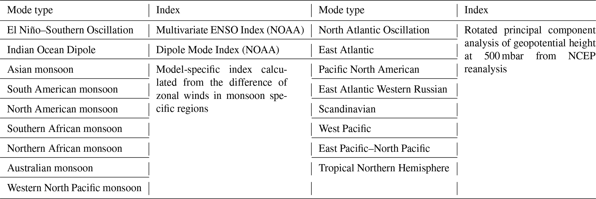
Monsoons included in this analysis are the Asian, South American, North American, southern African, northern African, Australian, and the western North Pacific. We calculate the monsoon index for each model used in this study based on the definitions of Yim et al. (2013), where the index is defined by the difference in zonal winds at 850 hPa between two monsoon-specific regions. See Table 2 in Yim et al. (2013) for more details. Because the MERRA-2 GMI and CCMI models included here are constrained or nudged to different reanalyses, the calculated monsoon index varies among the models, although the indices of a given monsoon from each model are highly correlated with one another (generally r2 > 0.9). Table 1 summarizes the climate modes and monsoons and the corresponding indices used here.
In addition to regression analysis, we also performed an empirical orthogonal function (EOF) analysis for tropospheric column OH (TCOH) and separately for each of the four layers described above. EOF analysis allows for the statistical determination of the spatial modes of OH variability and their variation with time without a priori knowledge of the controlling mechanisms (e.g., Barnston and Livezey, 1987). To perform the analysis, OH fields for each grid box were detrended by subtracting a linear fit to the time series over the 1980 to 2018 period to account for changes in background associated with long-term trends in OH. We report here only the first and second EOFs and their associated principal component time series as none of the other EOFs correlated spatially or temporally with any of the modes of climate variability discussed here.
2.2 MERRA-2 GMI simulation description
To understand the interannual variability of OH, we use the MERRA-2 GMI (Modern-Era Retrospective analysis for Research and Applications Global Modeling Initiative) simulation, publicly available at https://acd-ext.gsfc.nasa.gov/Projects/GEOSCCM/MERRA2GMI/ (last access: 21 April 2021). This is a run of the GEOSCCM model (Strode et al., 2019) constrained to meteorology from MERRA-2 (Gelaro et al., 2017) that uses the GMI chemical mechanism (Duncan et al., 2007; Oman et al., 2013; Gelaro et al., 2017). The GMI chemical mechanism includes approximately 120 species and 400 reactions, characterizing the photochemistry of the troposphere and stratosphere. The model was run from 1980 to 2018 at a resolution of C180 on the cubed sphere, equivalent to approximately 0.625∘ longitude × 0.5∘ latitude, with 72 vertical levels. The model was run in a replay mode (Orbe et al., 2017) and constrained to temperature, pressure, and winds from MERRA-2. Model output is available at daily and monthly resolutions, with hourly output available only for some local satellite overpass times. All data used in this work are monthly averaged unless otherwise indicated.
Anthropogenic emissions are from the Measuring Atmospheric Composition and Climate mega City (MACCity) inventory (Granier et al., 2011) for 1980–2010 and then from the Representative Concentration Pathway 8.5 (RCP8.5) scenario for 2011–2018. Biomass burning emissions are from the Global Fire Emissions Database (GFED) 4s inventory starting in 1997 (Giglio et al., 2013). Biomass burning emissions from before 1997 are calculated from scale factors derived from aerosol index data from the Total Ozone Mapping Spectrometer (TOMS) instrument, as described in Duncan et al. (2003b). Biogenic emissions are calculated online using the method described in Guenther et al. (1999, 2000), which is an early form of the Model of Emissions of Gases and Aerosols from Nature (MEGAN). A known high bias in isoprene emissions from MEGAN (e.g., Wang et al., 2017), could exacerbate low modeled OH in regions dominated by biogenic VOC emissions. Lightning NO emissions are based on the cumulative mass flux (Allen et al., 2010), with constraints from the Lightning Imaging Sounder (LIS)/Optical Transient Detector (OTD) v2.3 climatology (Cecil et al., 2014). Total, global lightning NO emissions are scaled to be 6.5 Tg N yr−1 for each year of the simulation, although emissions demonstrate significant interannual variability on the local scale. For example, over the tropical Pacific, an area we will investigate throughout this paper, peak emissions are 1.5 times higher than the minimum emissions over the time period studied here (Fig. S1 in the Supplement).
Methane concentrations are specified at the surface for four different latitude bands (90–30∘ S, 30∘ S–0∘, and 0∘–30∘ N, 30–90∘ N) at monthly resolution and advected throughout the troposphere. Methane data are from the NOAA Global Monitoring Division (GMD) surface network (Dlugokencky et al., 1994) and monthly values are interpolated from annual means.
Because CH4 is specified as a boundary condition, the model does not capture feedbacks (e.g., wetland or wildfire emissions) between CH4 emissions and climate modes beyond the extent to which these manifest in the observed methane surface concentrations. ENSO, for example, is known to affect atmospheric CH4 concentrations through changes in emissions from wetlands (Zhang et al., 2018; Melton et al., 2013) and biomass burning (Worden et al., 2013), although there is uncertainty in the magnitudes of these effects (Melton et al., 2013). On the global scale, however, these ENSO-induced changes in emissions do not significantly perturb background CH4. For example, during the 1997–1998 ENSO event, one of the largest on record, CH4 grew at a rate of approximately 15 ppbv yr−1 (parts per billion by volume per year) on top of a background of the order of 1700 ppbv (Nisbet et al., 2016). Because of this small perturbation and the dominance of CO as the primary OH sink over much of the globe (see Sect. 5), it is unlikely that the relationship between climate modes and OH would differ significantly with the inclusion of direct methane emissions in the simulation.
2.3 IGAC/SPARC Chemistry–Climate Model Initiative (CCMI) Phase 1 model simulations
To place the results from MERRA-2 GMI in the context of other models, we compare our simulation with those from the CCMI. The CCMI was conducted to help assess the ability of a suite of models to address various aspects of atmospheric chemistry, including trends in tropospheric ozone and the controlling mechanisms of OH (Morgenstern et al., 2017). Output from these models have already been used to assess various aspects of tropospheric OH (Zhao et al., 2019; Nicely et al., 2020), HCHO (Anderson et al., 2017), O3 (Revell et al., 2018; Dhomse et al., 2018), and meteorological variables (Orbe et al., 2020). Modeling groups conducted multiple runs, including a forecast scenario to 2100 and two hindcast scenarios, one with free-running meteorology and one, the specified dynamics (SD) scenario, in which models were either nudged to meteorological reanalyses or run as chemical transport models (Orbe et al., 2020).
We perform a similar analysis as with MERRA-2 GMI with four models that performed the CCMI SD run. We use the SD run, which spanned the years 1980–2010, instead of the other scenarios, to allow for more direct comparison among the CCMI models and with MERRA-2 GMI and observations from the satellite. We include only models that output data for all years between 1980 and 2010 and that have non-methane hydrocarbon chemistry in their chemical mechanisms. Models used here are WACCM (Solomon et al., 2015), CHASER (MIROC-ESM; Watanabe et al., 2011), a setup of EMAC with 90 vertical levels (EMAC; Jöckel et al., 2016), and MRI-ESM1r1 (Yukimoto et al., 2012). We omit CAM4Chem and a different setup of EMAC with 47 vertical levels because results for those models are essentially identical to WACCM and EMAC90, respectively. EMAC90 and CHASER were nudged to the ERA-Interim reanalysis, WACCM to the MERRA reanalysis, and MRI to the JRA-55 reanalysis. Sea surface temperatures (SSTs) and sea ice were prescribed in each model with the Hadley SST data set. Anthropogenic emissions were from the MACCity inventory, while lightning NOx was calculated online using model-specific parameterizations. Biomass burning emissions are from Granier et al. (2011), which incorporate a modified version of the RETRO inventory from 1980–1996 and GFEDv2 from 1997–2010 and are based on Lamarque et al. (2010). Monthly averaged CO emissions from this inventory in Indonesia, where biomass burning emissions are strongly affected by ENSO (e.g., Duncan et al., 2003a), are highly correlated (r2 = 0.79) in time with the GFED version 4s inventory used in the M2GMI simulation. Likewise, monthly averaged CO emissions over Indonesia from the two inventories agree within 35 %, on average. Further model details can be found in Orbe et al. (2020), Morgenstern et al. (2017), and references therein.
As with the MERRA-2 GMI analysis, we use monthly averaged output. For layer averaging, only EMAC90, WACCM, and MRI output a tropopause height, while no models output PBL height. To calculate the tropopause height for CHASER, we used the relationship between O3 and CO, as described in Pan et al. (2004). PBL height for all models was determined from the bulk Richardson number (Seibert et al., 2000).
While there has been some evaluation of the MERRA-2 GMI simulation (Ziemke et al., 2019; Strode et al., 2019), species in the simulation relevant to this study have not been investigated. As a result, we evaluate MERRA-2 GMI using in situ observations of OH and related species and remotely sensed observations of OH drivers in order to understand the effect any model biases could have on our results. In Sect. 3.1, we use in situ observations from the first two deployments of the Atmospheric Tomography (ATom) campaign to evaluate OH and CO over the remote Pacific and Atlantic Oceans. In Sect. 3.2, we also compare output to satellite observations of CO, H2O(v), and NO2 to evaluate the model over larger temporal and spatial scales.
3.1 Evaluation of MERRA-2 GMI with in situ observations
During the ATom campaign, a suite of air quality and climate-relevant trace gases and aerosols were measured throughout the remote Pacific and Atlantic. During each of the deployments, aircraft transected the Pacific from Alaska to New Zealand, went around Tierra del Fuego, and traveled north over the Atlantic to Greenland. Each flight consisted of a series of ascents and descents, allowing for vertical profiling across most latitudes of the remote Pacific and Atlantic Oceans. The combination of the flight track and the repetition across seasons provided unprecedented sampling of many trace gases, including OH. As part of the ATom campaign, a limited subset of species, including OH and CO, from the MERRA-2 GMI simulation were output hourly for the duration of ATom 1 (July–August 2016) and ATom 2 (January–February 2017) only, allowing for direct comparison to the in situ observations. Only daily or longer resolution output is available for the other deployments, and, as a result, we focus our analysis on these first two deployments.
Observations used here include OH (Brune et al., 2020) and CO (Santoni et al., 2014), with 2σ uncertainties of 35 % and 3.5 ppbv, respectively. Data have been averaged to a 5 min time base and filtered for biomass burning influence, defined as times when concentrations of HCN and CO are both above the 75th percentile for the individual ATom deployments. We omit the biomass-burning-influenced parcels because small differences in measured and modeled winds could result in misplacement of modeled biomass burning plumes, resulting in unrealistically large differences in OH. Inclusion of the biomass-burning-influenced parcels does not significantly change the model bias but does degrade the correlation. For comparison of the observations to MERRA-2 GMI, hourly data were output by the model and then bilinearly interpolated in the horizontal and linearly interpolated in time and in the vertical to the in situ observation time and location.
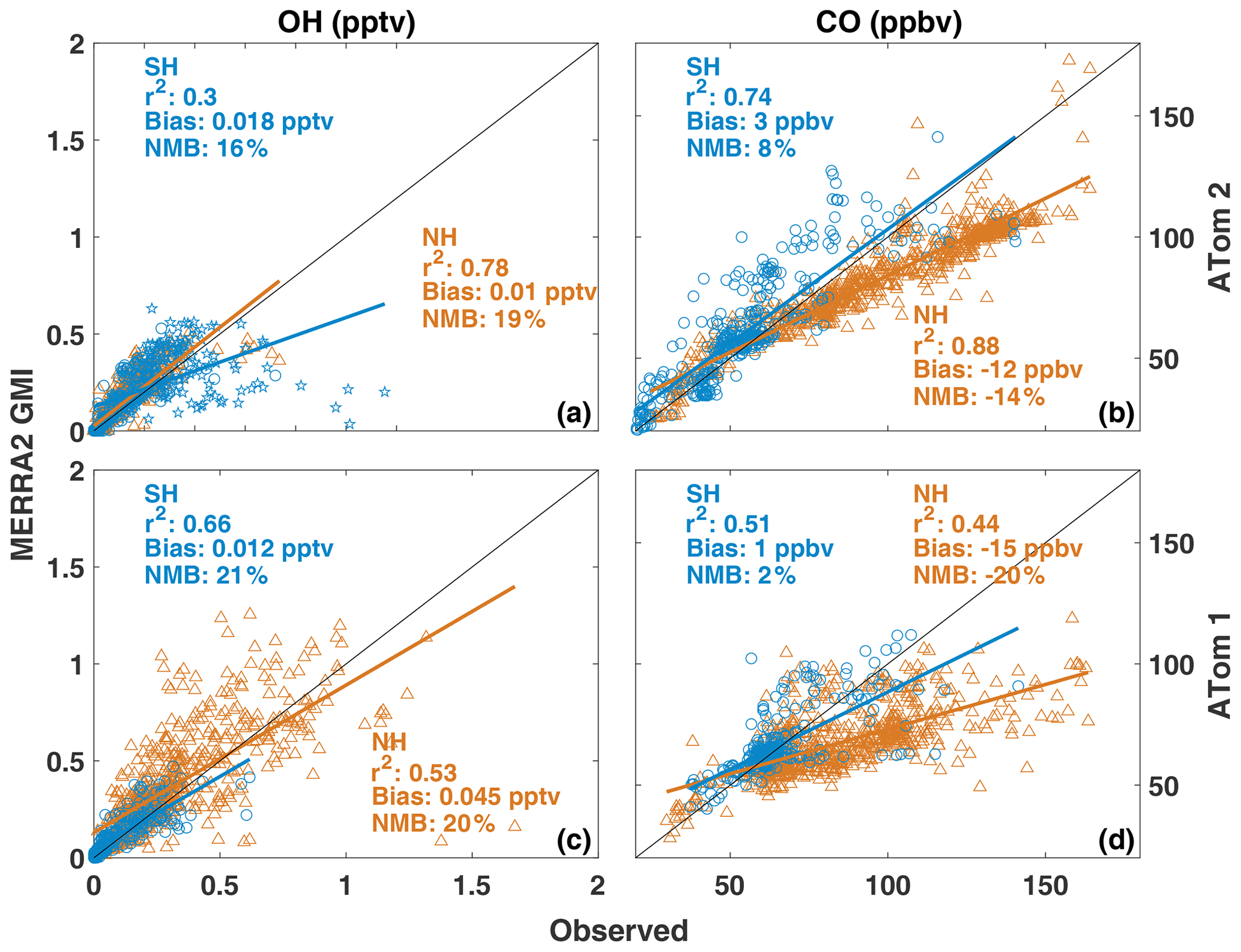
Figure 1Regression of observed OH (a, c) and CO (b, d) from ATom 2 (boreal winter 2017; a, b) and ATom 1 (boreal summer 2016; c, d) against hourly output from MERRA-2 GMI interpolated to the ATom flight track. Data from the Southern (blue circles) and Northern (orange triangles) hemispheres are shown, along with the r2, bias, and normalized mean bias (NMB) for each hemisphere. Observations and model output have been filtered for biomass burning influence. Observations of continental outflow from New Zealand and South America from ATom 2 are indicated by blue stars.
MERRA-2 GMI has a OH high bias of approximately 20 % (Fig. 1a) when compared to observations from ATom 2. A regression of measured and modeled OH shows a moderate to high correlation in both the Southern Hemisphere (SH) and NH, with r2 values of 0.30 and 0.78, respectively. Normalized mean biases (NMBs) relative to the observations are within measurement uncertainty in both the NH (19 %) and SH (16 %), with nearly identical high biases during the summer deployment of ATom 1 (Fig. 1c). The comparatively poorer model performance for OH in the SH is being driven by continental outflow from South America and New Zealand. When data from these regions are omitted (Fig. 1a; blue stars), the correlation for the SH increases to 0.63 and the NMB is 22 %. The limited model output at hourly resolution does not allow for a determination of the cause of this disagreement in continental outflow regions. In the case of South America, however, a known high bias in modeled isoprene, resulting in extremely low OH over the Amazon, is consistent with the disagreement between the simulation and observations.
Agreement between observed and modeled CO shows a strong hemispheric dependence, with a NMB of −14 % in the NH (i.e., the model is lower than observations by 14 %) and 8 % in the SH during ATom 2, although both hemispheres have a strong correlation (r2 > 0.7). While agreement in the SH improves in ATom 1, with a NMB of 2 % (Fig. 1d), the model underestimate in the NH is even more pronounced (NMB = −20 %). This NH low bias in CO is a well-known problem in global chemistry models (e.g., Naik et al., 2013; Stein et al., 2014; Travis et al., 2020) and could be a contributing factor in the overestimate in OH, as CO is the dominant global OH sink.
Comparison of the MERRA-2 GMI simulation to in situ observations demonstrates that the model captures the spatial variability of OH and its predominant global sink, CO, in the remote atmosphere during both the NH summer and winter, with the exception of OH off the coast of South America and New Zealand. The poorer agreement between measured and modeled OH in regions of fresh, continental outflow suggests that modeled relationships between climate modes and OH in these regions might be more uncertain than in the remote atmosphere. This lack of agreement does not significantly affect the results discussed in this work, as the majority of the relationships found between OH and modes of climate variability discussed in Sects. 4 and 5 are centered in the remote atmosphere.
3.2 Evaluation of MERRA-2 GMI with satellite observations
While there are no remotely sensed observations of tropospheric column OH (TCOH), there are satellite observations of OH drivers. Comparing these observations to MERRA-2 GMI allows for model evaluation over larger spatial and temporal scales than with ATom. Satellite data used here include tropospheric CO columns from the Measurement Of Pollutants In The Troposphere (MOPITT) instrument, H2O(v) from the Atmospheric Infrared Sounder (AIRS), and tropospheric NO2 from the Ozone Monitoring Instrument (OMI). AIRS is on the Aqua satellite, with a daily local overpass time of approximately 13:30 LT (local time; applicable to all times given herein). We use the monthly averaged, level 3, version 6 standard physical retrieval (Susskind et al., 2014) from 2003 to 2018. For MOPITT CO on the Terra satellite, we use the level 3, version 008 retrieval that uses both near- and thermal-infrared radiances (Deeter et al., 2019) from 2001 to 2018. MOPITT has a daily local overpass time of approximately 10:30. Both satellite products have a global horizontal resolution of 1∘ × 1∘. We also use the OMI NO2 version 4, level 3 product (Lamsal et al., 2021) from 2005 to 2018. Data have been regridded to 1∘ × 1∘ horizontal resolution. OMI is located on the Aura satellite and, as with AIRS, has a local overpass time of approximately 13:30.
For comparison of the satellite retrievals to MERRA-2 GMI, we use monthly fields of the model variables output at the satellite overpass time. For CO, where averaging kernel and a priori information are available for the level 3 MOPITT data, we convolve the model output with these variables so that direct comparison between satellite and model are possible. While shape factors and scattering weights for the OMI NO2 retrieval are unavailable for the level 3 data, shape factors for the OMI NO2 retrieval are determined from a similar setup of the GEOSCCM model, also employing the GMI chemical mechanism and MERRA-2 meteorology. Applying the satellite shape factors to the simulation discussed here would therefore not result in significant changes in the modeled NO2. Finally, for AIRS H2O(v), averaging kernel information was unavailable for the level 3 data, so numerical comparisons between satellite and model should be regarded as more qualitative than quantitative.
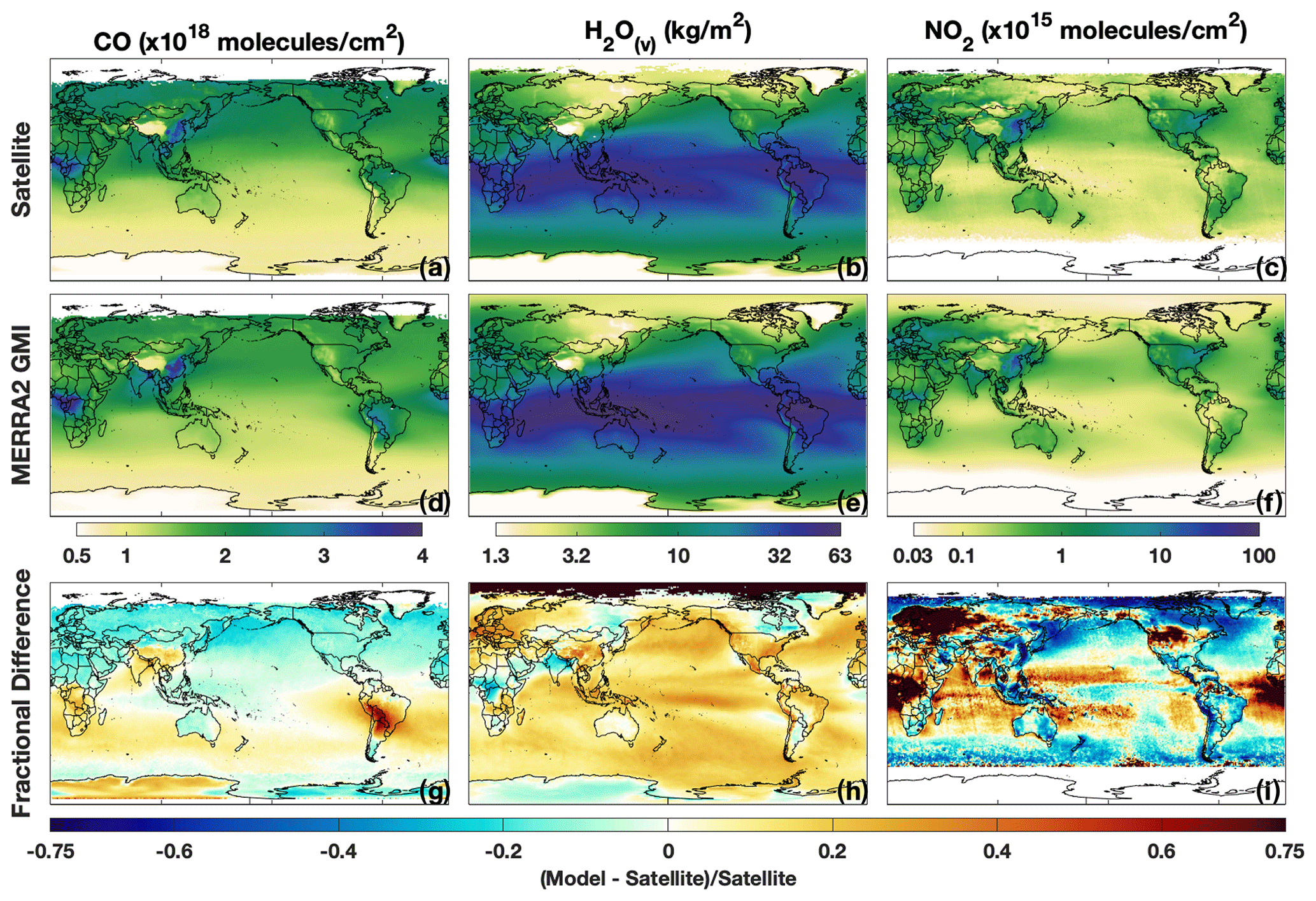
Figure 2Tropospheric column CO (a, d, g), H2O(v) (b, e, h), and NO2 (c, f, i) from MOPITT, AIRS, and OMI, respectively (a–c), and MERRA-2 GMI (d–f) for DJF (December–February). For the satellite retrievals and model, data are averaged over the time range described in the text for each instrument. The fractional difference between MERRA-2 GMI and the satellite is shown in (g–i).
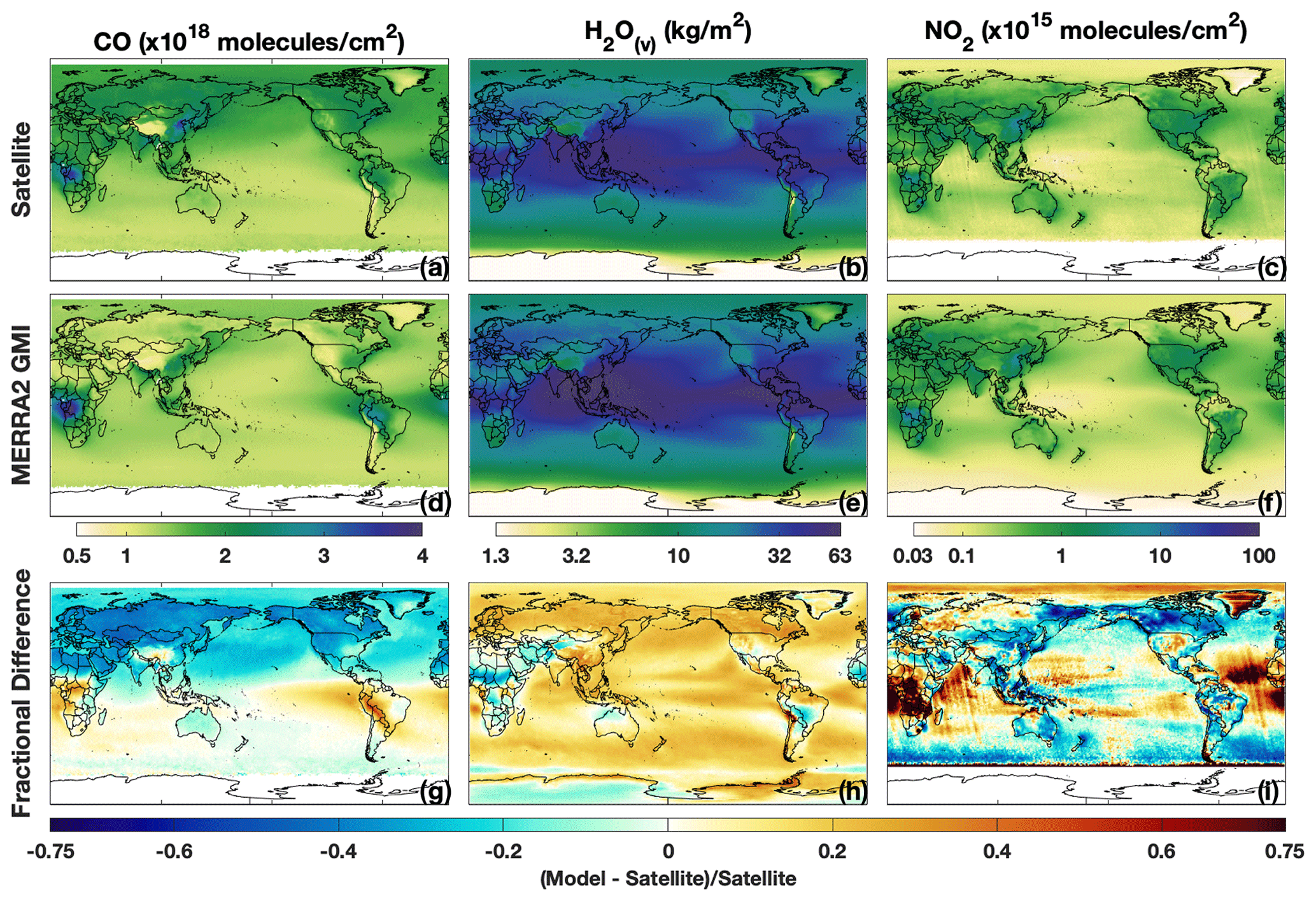
Figure 3Same as Fig. 2 except for JJA (June–August).
When compared to MOPITT in boreal winter (i.e., DJF – December–February), tropospheric column CO from MERRA-2 GMI (Fig. 2; first column) shows similar results to that found through comparison to the in situ observations, namely a low bias in the NH (9 %) and high bias in the SH (7 %). Differences over the tropical Pacific, an area that will be shown later to have a strong relationship between ENSO and OH, are generally less than 10 %, while a noticeable high bias exists over parts of South America. Results for June–August (JJA) are spatially similar (Fig. 3), with a NH low bias of 20 % and overestimates of column CO, averaging 45 %, in the SH. These areas of high bias over South America likely result from the high bias in isoprene emissions, as discussed in Sect. 2.2, that would lead to unrealistically high in situ production of CO.

Figure 4The fractional difference in zonal mean H2O(v) between MERRA-2 GMI and AIRS for the different AIRS pressure layers for DJF. Positive numbers indicate a high bias in the model.
MERRA-2 GMI captures the spatial distribution of H2O(v), although the model is biased high in both the column and throughout much of the troposphere. Overestimates in column H2O(v) are ∼ 14 % in both DJF (Fig. 2h) and JJA (Fig. 3). These overestimates extend over most of the world's oceans, and only small regions over northern India, central Africa, eastern Russia, and eastern Canada show any underestimate in H2O(v). Fractional differences in H2O(v) between MERRA-2 GMI and the different AIRS pressure levels are most pronounced in the tropical UT (Fig. 4). At pressures greater than 700 hPa, modeled H2O(v) is generally within 10 % of the observations, while for pressures less than 500 hPa, modeled H2O(v) in the equatorial region disagrees with observations by 55 % on average.
Agreement between observed and modeled NO2 is weaker than for the other species examined here. While MERRA-2 GMI appears to capture the regions with local NO2 maxima – notably those over central Africa, eastern China, and the northeastern United States – the magnitudes frequently differ. The simulation shows a significant high bias over central Africa and the equatorial Atlantic of the order of 100 %, suggesting that biomass burning emissions of NOx, the dominant NO source in this region, are too high. In contrast, concentrations over eastern Asia are too low in the model, suggesting errors in the anthropogenic emissions inventory and/or in the NOx lifetime. Strode et al. (2019) also evaluated NO2 in MERRA-2 GMI, comparing trends in tropospheric column NO2 over the eastern US and eastern China in MERRA-2 GMI and OMI. They found that, although trends were similar between the simulation and observations in both regions, the magnitude of the trends differed, likely due to errors in the MACCity emissions inventory.
As with the in situ observations, comparison between MERRA-2 GMI and satellite retrievals demonstrates that the simulation is able to capture the distribution of the chemical drivers of OH in remote regions which tend to exhibit the strongest relationship between OH and climate modes (see Sect. 4). These results lend confidence to the analysis described in Sects. 4 and 5 and suggest that the findings in remote regions are likely applicable to the actual atmosphere. The large disagreement between the simulation and observed column CO and NO2 in regions that are significantly impacted by biomass burning and/or biogenic emissions suggests, however, that modeled relationships of chemical species with modes of climate variability in these regions should be viewed with caution. We further evaluate the ability of the simulation to capture the relationship between ENSO and CO, H2O(v), and NO2 using satellite observations in Sect. 5.1.2.

Figure 5Regions that show a significant correlation (absolute value of r > 0.5) between a NH mode (purple), monsoon (light blue), ENSO (green), or IOD (orange) and TCOH for each season in the MERRA-2 GMI simulation. Regions with TCOH less than 1 × 10¹¹ have been hatched out.
When considered in concert, the modes of climate variability evaluated here (i.e., ENSO, the IOD, and NH modes), along with monsoons, explain a substantial fraction of the simulated tropospheric OH interannual variability over 19 %–40 % of the global troposphere by mass, depending on season. Figure 5 highlights regions that show significant correlation between TCOH and the NH modes (purple), monsoons (light blue), ENSO (green), and the IOD (orange) for each season in MERRA-2 GMI output. In all seasons, correlation with ENSO has the largest spatial extent, but in DJF and MAM (March–May), for example, the eight NH modes can explain TCOH variability over large swaths of the NH, comprising 10 % of global, tropospheric mass. In JJA, the combination of the different climate modes and monsoons has the smallest spatial coverage (19 % of the global tropospheric mass), while the IOD, consistent with its seasonal variability, only has a widespread correlation with TCOH during SON (September–November). Similar patterns are found for the individual layers (Fig. S2 in the Supplement).
Below, we examine the relationships between tropospheric OH and the various modes of climate variability demonstrated in Fig. 5. First, in Sect. 5, we show that El Niño events lead to global reductions in tropospheric OH, with changes being driven by decreased secondary production in the UFT that more than compensates for increased primary production in the PBL. In Sect. 6, we demonstrate that the effects on OH from NH modes of variability, the IOD, and some monsoons have limited spatial scales, as compared to ENSO, but can significantly alter local OH distributions. In both sections, we also compare simulations from MERRA-2 GMI to simulations from the CCMI, demonstrating that the relationship between OH and climate modes is robust among multiple models.
To understand the relationship between OH, its drivers, and ENSO, we first investigate the OH production rate. In the MERRA-2 GMI simulation, the OH production rate is primarily dependent on Reactions 1–4, where O1D is produced from the photolysis of tropospheric O3. In the free troposphere, these four reactions comprise at least 95 % of OH production in the tropics, on average, and at least 90 % in the PBL. Only in the regions with large biogenic emissions (e.g., South America and central Africa) do other reactions contribute more than 15 % of the total OH production in the PBL. As will be shown, the effects of ENSO on OH are primarily focused away from these regions, so we restrict our analysis to the reactions (R1)–(R4).
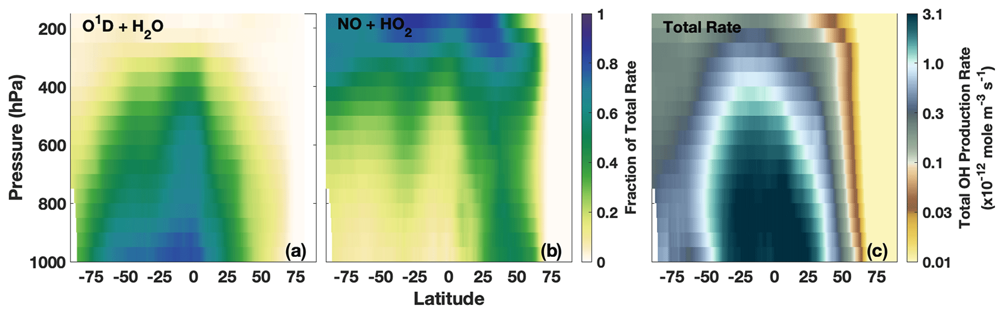
Figure 6Zonal mean of the fractional contribution of the O1D + H2O (a) and NO + HO2 (b) reactions to the total OH production rate and the total OH production rate (c) for El Niño events (MEI > 0.5) for DJF, averaged over 1980–2018.
During El Niño events, the dominance of these individual reactions in producing OH varies with altitude. We focus our analysis on DJF throughout Sect. 5 because that is the season with the largest impact of ENSO on OH, as shown in Fig. 5. Figure 6 shows the zonal mean of the fraction of total OH production from the H2O + O1D (Fig. 6a) and NO + HO2 (Fig. 6b) reactions as well as the total OH production rate (Fig. 6c) during El Niño events in DJF. While the production rates along these pathways vary with the ENSO phase, as discussed in Sects. 5.2 and 5.3, the relative importance of the individual reactions is similar during neutral and La Niña events (not shown) and is in agreement with previous model studies (e.g., Spivakovsky et al., 2000).
The H2O + O1D reaction is dominant from the surface to about 800 hPa through much of the SH and the tropics, while, near the surface, the NO + HO2 reaction only has large impacts in the NH midlatitudes. This influence of NOx in the NH midlatitudes extends through much of the troposphere. In the UFT, this reaction is the greatest contributor to total OH production at all latitudes except the NH polar region, where the HO2 + O3 reaction dominates during polar night (Fig. S3 in the Supplement). Total OH production in the polar regions, however, is orders of magnitude lower than in the tropics. Outside of the polar regions, the HO2 + O3 and H2O2 photolysis reactions generally contribute between 10 % and 30 % of the total rate (Fig. S3). The dominant OH sink throughout the troposphere is CO, which is responsible for a 50 % or greater OH loss at all tropospheric pressures and latitudes (Fig. S4 in the Supplement) during El Niño events. Because of the differing importance of the individual OH production reactions with altitude, we first examine the relationship between OH and ENSO for TCOH (Sect. 5.1) and then separately for the PBL (Sect. 5.2) and the UFT (Sect. 5.3). Finally, in Sect. 5.4, we investigate the MFT and LFT, where the effects of ENSO on OH are more limited.
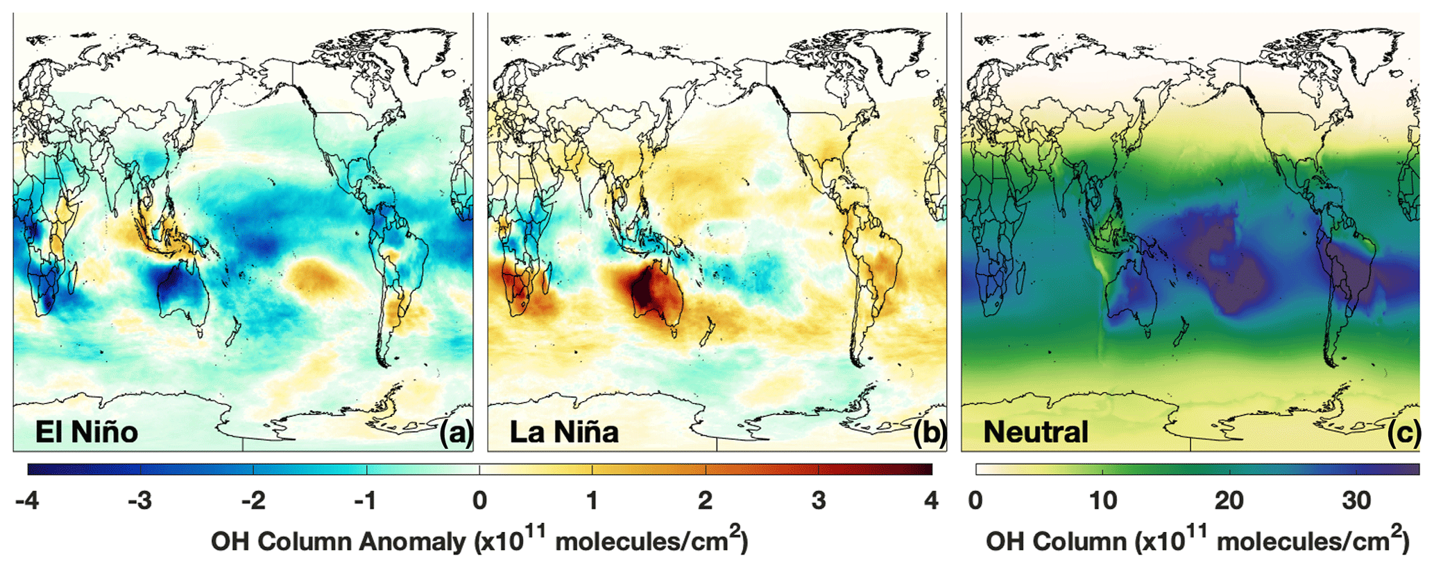
Figure 7Absolute difference in TCOH between El Niño events and neutral events (a) for DJF, averaged over 1980–2018. El Niño and neutral events are defined as a season having an MEI value greater than 0.5 or an MEI value between −0.5 and 0.5, respectively. The analogous plot for La Niña events (MEI less than −0.5) is also shown (b). Panel (c) shows the average OH column for neutral events. The 1980–2018 time period includes 11 El Niños, 12 La Niñas, and 15 neutral events in DJF.
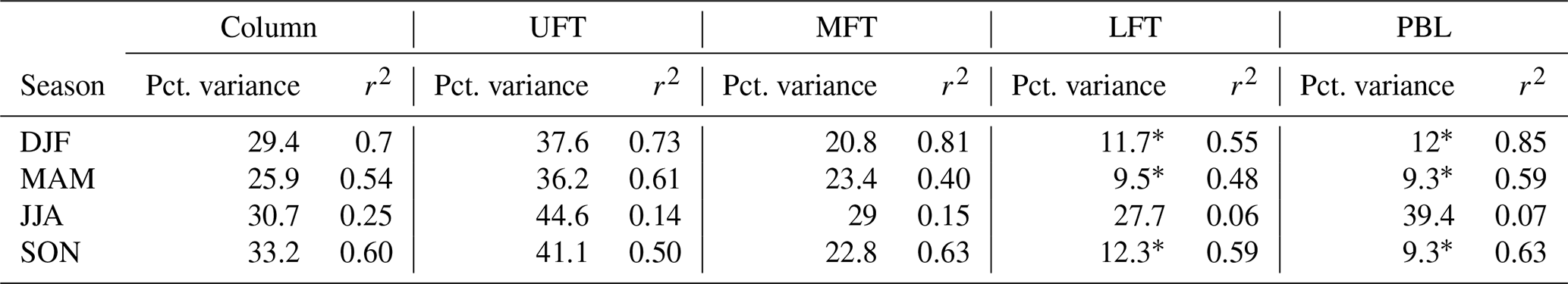
Table 2For each season, we show the r2 of the correlation of the temporal component of the EOF that has the highest correlation with the MEI for TCOH and for OH in each layer. In addition, we also indicate the percent (Pct.) of the total spatial variance explained by that EOF. With the exception of the values indicated by an asterisk (∗), the first EOF has the highest correlation with the MEI. Those indicated with an asterisk (∗) are the second EOF.
5.1 Tropospheric column OH
5.1.1 The relationship between simulated TCOH and ENSO
As shown in Fig. 7, TCOH decreases by 3.3 % during El Niño events (relative to neutral events) equatorward of 30∘ in DJF and is characterized by widespread decreases in the tropics and subtropics, especially in northern Australia and west–central and southern Africa. Regional increases are found over eastern Africa, the east–central Pacific, southern South America, and Indonesia. Maximum decreases in TCOH are of the order of 4.5 × 10¹¹ (∼ 10 %–15 %) and are centered over northern Australia, while maximum increases in TCOH (∼ 2.5 × 10¹¹ ) are centered over Sumatra.
During La Niña events, TCOH increases relative to neutral events over much of the globe, although the changes are not necessarily symmetric with those seen during El Niño events. Increases over Australia are of the order of 1 to 2 × 10¹¹ , on par with the decreases seen during El Niño, but the changes during La Niña are centered over western Australia and the Indian Ocean. Over the Pacific, the magnitude of the OH increase is lower (of the order of 0.5 to 1 × 10¹¹ ) than the decreases found during El Niño, and some regions off the coast of Hawaii and Papua New Guinea show decreases during both ENSO phases. Besides these two regions, there are also significant decreases in OH over eastern Africa and in the southern portion of South America.
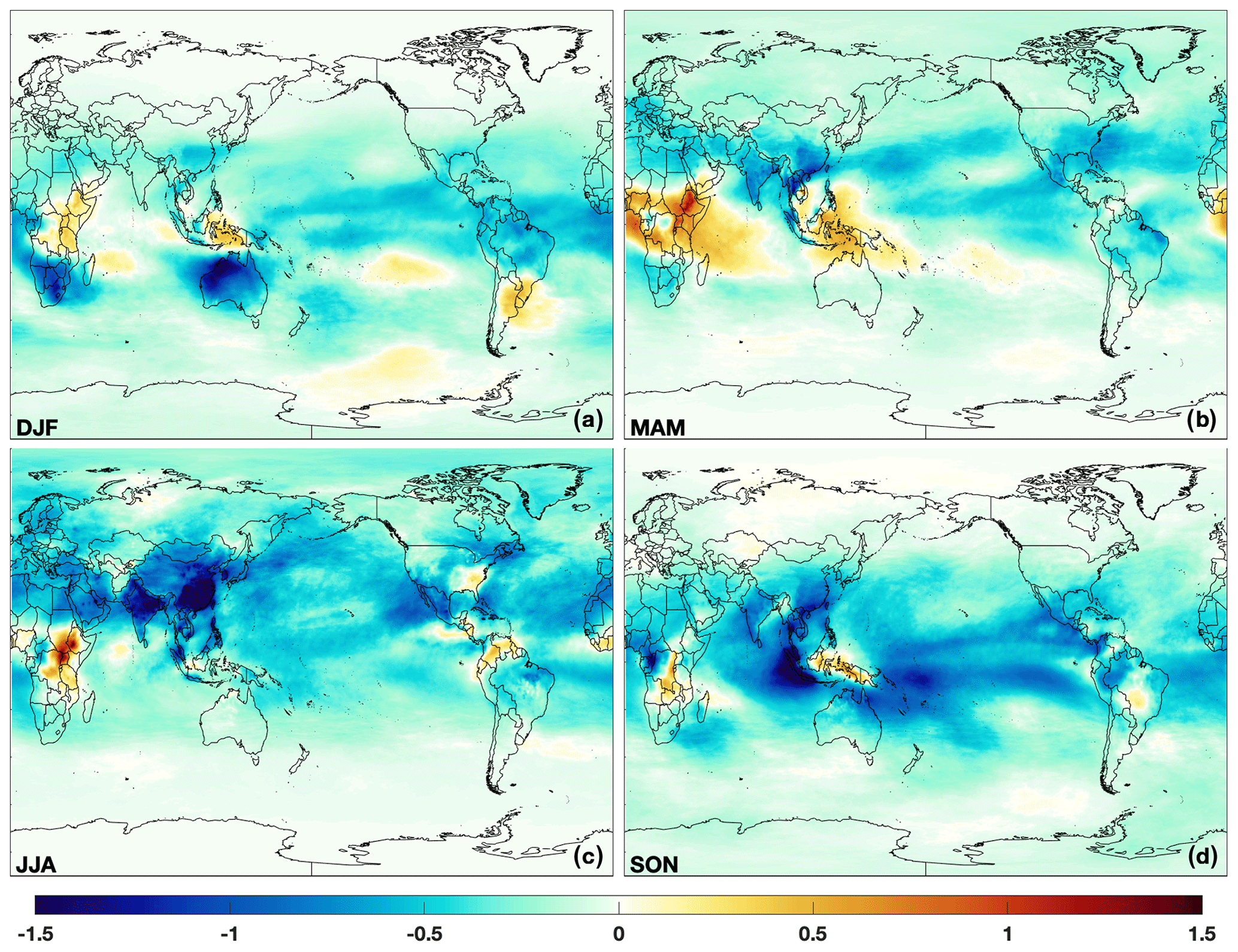
Figure 8The first EOF of TCOH from MERRA-2 GMI for DJF (a), MAM (b), JJA (c), and SON (d).
Consistent with these widespread changes in TCOH, EOF analysis demonstrates that, over most seasons, with JJA being the notable exception, ENSO is the dominant mode of OH variability. Figure 8 shows the spatial component of the first EOF of TCOH for the four seasons. While EOF analysis does not quantify changes in column content, it does highlight, for each mode of variability, regions where changes in TCOH are most prominent. For DJF, the first EOF (Fig. 8a) is almost identical to the composite figure showing OH anomalies during El Niño (Fig. 7a). Likewise, the temporal component of the first EOF strongly correlates with the MEI (r2 = 0.70; Table 2). In DJF, the first EOF is responsible for 29 % of the total spatial variance for TCOH. Although ENSO is the dominant mode, however, 70 % of the spatial variance is still unexplained. In JJA, ENSO influence on OH is much weaker, with a correlation between the first EOF and TCOH of r2 = 0.25, consistent with the seasonal cycle of ENSO.
While the spatial pattern of the EOF varies seasonally (Fig. 8), ENSO shows similar levels of correlation to the temporal component of the first EOF in MAM and SON as for DJF, with r2 values of 0.54 and 0.60, respectively. Likewise, the spatial patterns of the first EOF of TCOH for these seasons are similar to the composite figures showing OH anomalies during El Niño (Fig. S5 in the Supplement). For MAM, the EOF again shows regions with a negative sign over much of the Northern Hemisphere, with the largest magnitude centered over the Pacific Ocean, India, and the Atlantic coast of the United States. Regions with an opposite sign include the Maritime Continent and much of central Africa. In SON, almost all of the tropics show some response, with major centers off the east coast of Papua New Guinea and off the west coast of Sumatra. In addition, there is a larger response over the Indian Ocean than for other months, also evident in the regression of TCOH with the MEI, suggesting the possible influence of the IOD, which is correlated with ENSO (r2 = 0.30). This seasonal component in the strength of the relationship between the EOF and the MEI is also reflected in the correlation analysis (Fig. 5), where the area of correlation between TCOH and the MEI maximizes in DJF and minimizes in JJA.
5.1.2 The relationship between TCOH drivers and ENSO
To understand the factors driving ENSO-related changes in TCOH, we also investigate the relationship between OH precursors and ENSO. Figure 6 demonstrates that the O1D + H2O and NO + HO2 reactions control zonal mean OH production in the tropics. As a result, we investigate the relationship between the tropospheric column H2O(v), CO, NO2, and ENSO using both MERRA-2 GMI output and satellite retrievals. We use NO2 here, instead of NO, because of its observability from space, although simulated NO demonstrates similar spatial correlation patterns with the MEI as simulated NO2.
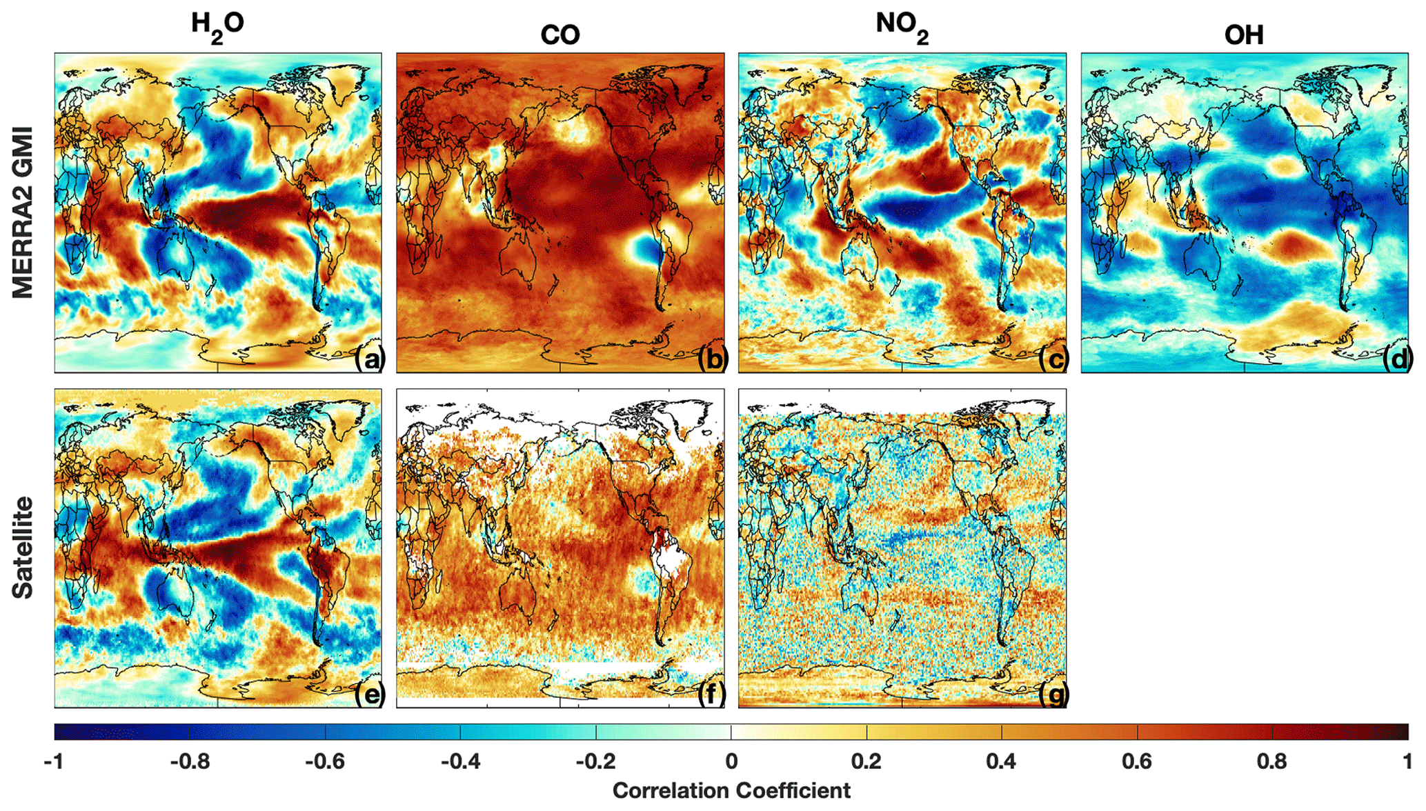
Figure 9Regression of tropospheric column H2O(v) (a), CO (b), NO2 (c), and OH (d) from MERRA-2 GMI (top) and satellite retrievals from AIRS (e), MOPITT (f), and OMI (g) against the MEI for DJF over the satellite lifetime.
Regression of total column H2O(v) from AIRS against the MEI (Fig. 9e) reveals a tripole pattern over the Pacific Ocean, with an area of positive correlation throughout much of the equatorial Pacific Ocean and areas of anti-correlation poleward of this region, in agreement with previous work (e.g., Shi et al., 2018). Each of these areas is well captured by the MERRA-2 GMI simulation (Fig. 9a), showing nearly identical spatial patterns and strength of correlation over most of the globe. This relationship between H2O(v) and ENSO can be explained by the increased convective uplifting in the equatorial Pacific and the associated increased subsidence poleward of this region during El Niño events. While the anticorrelation between H2O(v) and the MEI over Australia and southern Africa is consistent with the decrease in TCOH over these regions during El Niño events (Fig. 7), the positive correlation between H2O(v) and the MEI over the equatorial Pacific suggests there must be competing effects from other OH drivers in order to explain the decreases in TCOH in this region.
Simulated tropospheric column NO2 is strongly anti-correlated with ENSO over the equatorial Pacific, indicating a suppression of OH production when the MEI is positive (El Niño), which is consistent with Fig. 7. Column NO2 exhibits the opposite correlation pattern to that of H2O(v) over the Pacific, with decreases in NO2 in regions with increased H2O(v) and vice versa. The similarities in the spatial correlation patterns for NO2 and H2O(v) with the MEI suggests that convection is also at least partially driving the changes in NO2 in the equatorial Pacific. Changes in the Walker circulation associated with El Niño events have been shown to redistribute O3 in the tropics, resulting in a dipole pattern over the western and central Pacific (Oman et al., 2011). Analysis of vertical winds and the NO2 anomaly suggests a similar mechanism for NO2.
Correlations between OMI NO2 and the MEI suggest similar relationships as found in the MERRA-2 GMI simulation, although the correlations are not as robust as for the other satellite variables examined here. This is likely because tropospheric NO2 columns over the ocean are frequently at or below the instrumental average noise (5 × 10¹⁴ ). As with the simulation, OMI suggests broad regions of anti-correlation between ENSO and NO2 in the equatorial Pacific and the Gulf of Alaska as well as a region of positive correlation in the extra-tropical NH Pacific. These results demonstrate that, with enough temporal and spatial averaging, OMI is capable of capturing the variability in tropospheric NO2, even in remote regions with low concentrations.
Tropospheric column CO and the MEI are positively correlated over most of the globe in both MERRA-2 GMI and in MOPITT (Figs. 9b and f, respectively), suggesting strong increases in CO during El Niño events. This increase in CO is associated with increased biomass burning, particularly in Indonesia, and is consistent with the modeled decrease in OH (e.g., Duncan et al., 2003a) and with the widespread decrease in TCOH over much of the tropics.
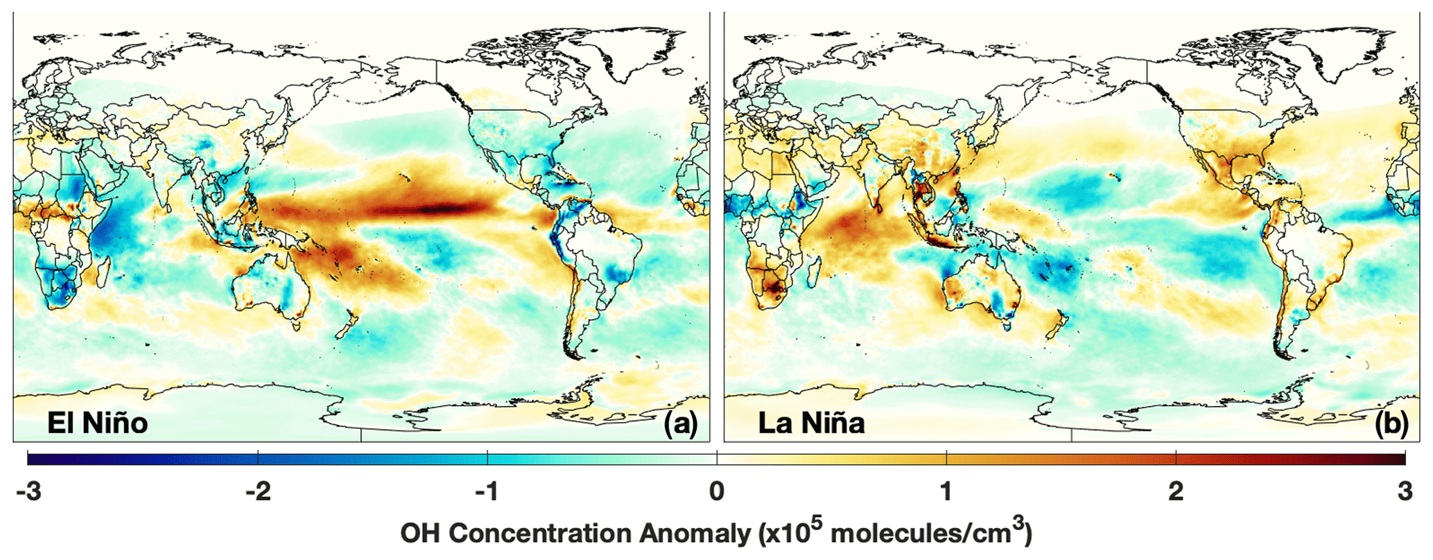
Figure 10Same as panels (a) and (b) of Fig. 7 except for the PBL level.
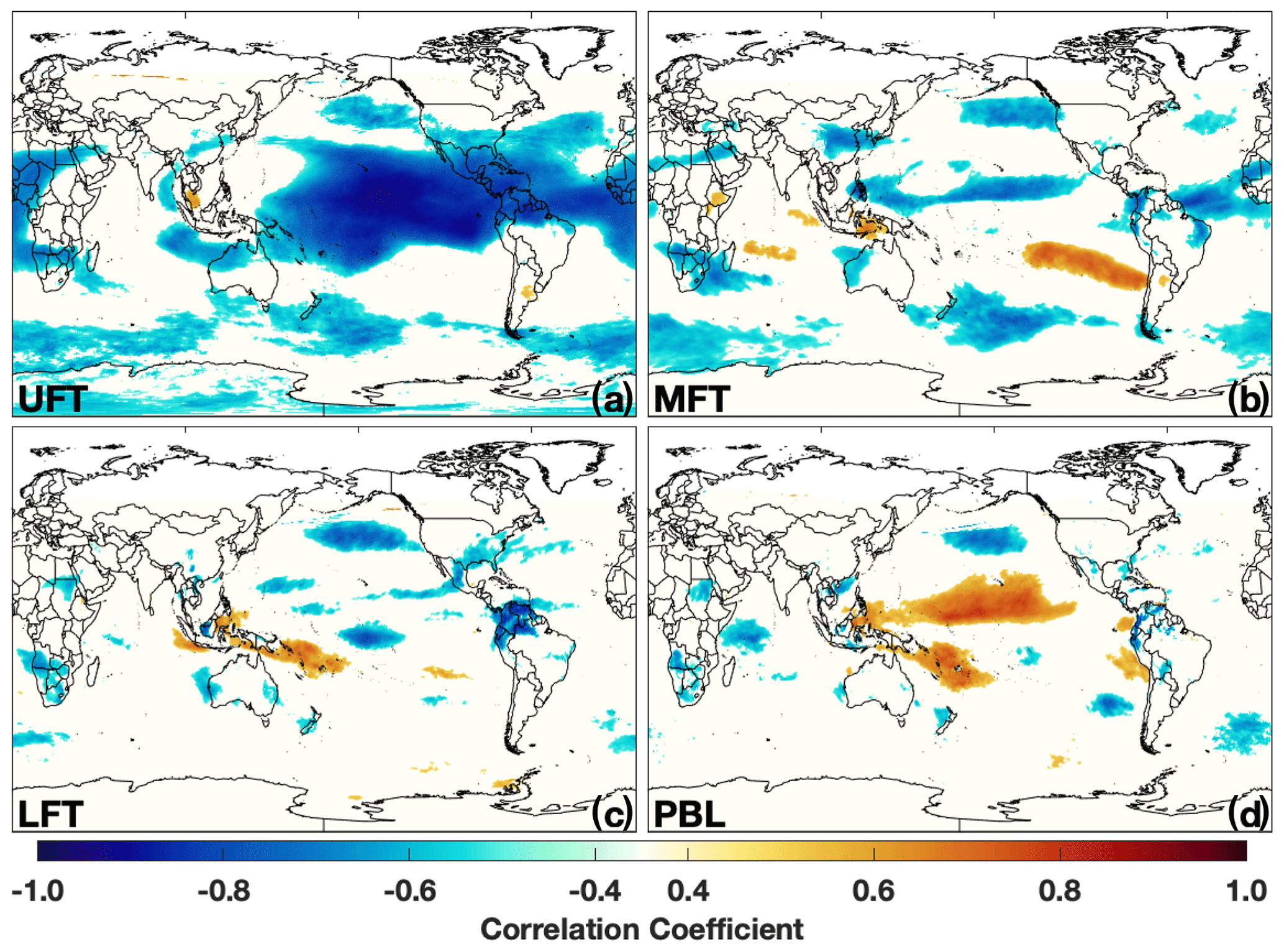
Figure 11Correlation of OH from MERRA-2 GMI with the MEI for the different atmospheric layers in DJF.
5.2 The planetary boundary layer
5.2.1 The relationship between PBL OH and ENSO
In contrast to the tropospheric column (Fig. 7), mean mass-weighted OH (e.g., Lawrence et al., 2001) in the PBL increases globally by 1 % during El Niño events (Fig. 10), although regional differences are significantly larger. PBL OH exhibits an area of strong positive correlation with the MEI (Fig. 11d) over the central Pacific, marked by increases in concentrations of the order of 2–3 × 10⁵ , approximately 15 % higher than concentrations in neutral events. Changes in the PBL during La Niña are smaller, with localized concentration decreases of about 5 %–10 % over the tropical Pacific (Fig. 10b). Regions with significant correlation between PBL OH and the MEI are distinctly smaller than in the UFT (Fig. 11) and for TCOH (Fig. 5a), further emphasizing the comparatively limited spatial effects of ENSO in the PBL.
The more geographically limited changes in OH, shown by the composite and regression analyses, are consistent with EOF analysis. During all seasons except JJA, ENSO correlates more strongly with the second EOF for the PBL (Table 2), suggesting another mechanism is the dominant mode of variability. The spatial pattern of the second EOF for PBL OH varies markedly across seasons (Fig. S6 in the Supplement), with the largest signal over the tropical Pacific during DJF and MAM and over Indonesia in SON. In general, the r2 with ENSO is 0.5 or higher, and the mode contributes approximately 10 % of the total spatial variance, although correlation in JJA (r2 = .07) is negligible.

Figure 12Correlations of the MEI with the production rate of OH from the H2O + O1D reaction (a) for DJF and the total OH production rate, as defined in the text, (b) for the PBL level are shown.
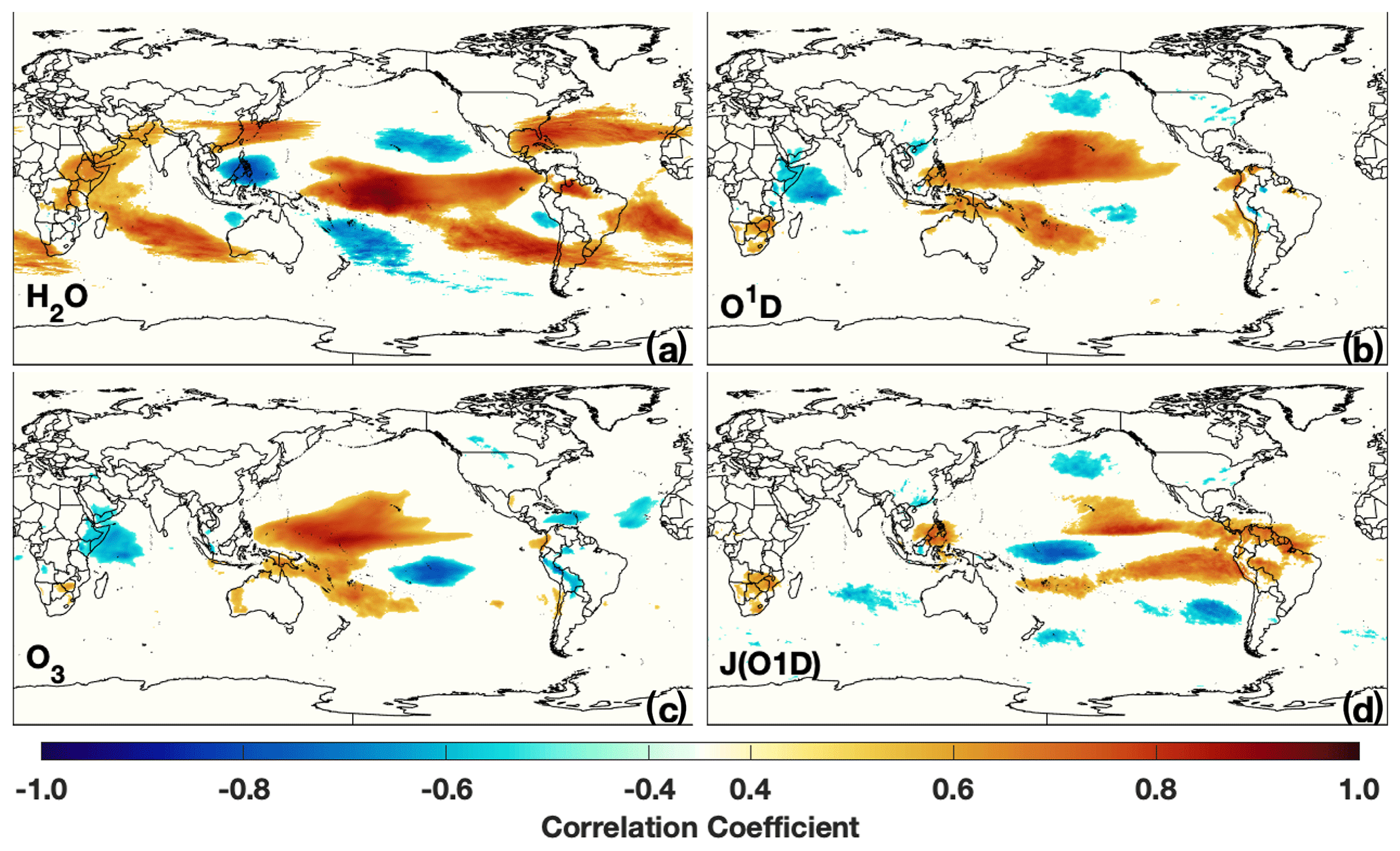
Figure 13Correlation of the indicated species with the MEI for the PBL level for DJF.
In contrast to the ENSO-related EOFs, the first EOF (Fig. S7 in the Supplement) for the DJF PBL layer reveals a spatial pattern much more limited to continental regions and areas of continental outflow, suggesting that this mode of variability is potentially reflective of long-term emission trends in both anthropogenic and biomass burning emissions. This is more evident in the first EOF for JJA, where the spatial pattern shows opposite signs over regions with known net emissions reductions (the United States, portions of Europe, and Japan) and those with known net emissions increases (China, India, and the Middle East) over the 1980–2018 period examined here.
5.2.2 The relationship between PBL OH drivers and ENSO
Approximately 80 % of the zonal mean OH production in the tropical PBL during El Niño events is from the H2O + O1D reaction (Fig. 6a). Figure 12 shows the correlation of the MEI against both OH production from this reaction and the total OH production rate for the PBL. Similar plots for the other OH production reactions are shown in Fig. S8 in the Supplement. The nearly identical regression pattern for the H2O + O1D and the total production rate with the MEI demonstrates that changes in this reaction are driving changes in OH in the tropics during El Niño events.
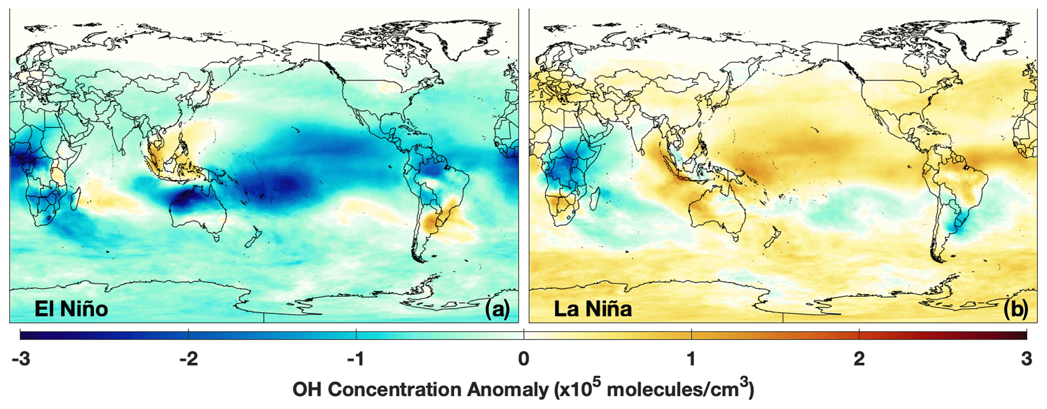
Figure 14Same as Fig. 7 except for the UFT.
To understand the relationship between the OH production rate and ENSO in the PBL, we examine the changes in H2O(v) and O1D (Fig. 13). The spatial correlation of H2O(v) and the MEI in the PBL exhibits a tripole pattern similar to that seen in the tropospheric column (Fig. 9a). While H2O(v) is correlated with the MEI in the equatorial Pacific, which would lead to increases in OH production, H2O(v) is anti-correlated with the MEI near the Hawaiian Islands and in the south Pacific, which would lead to decreased OH production in these regions. Because OH increases in these areas during El Niño events, the decreased H2O(v) is offset by increases in O1D, resulting in a net positive correlation of the total OH production rate.
Changes in O1D and its photochemical drivers, O3 and the rate of O3 photolysis to O1D (J(O1D)), are driving the ENSO-related changes in OH in the PBL. O1D shows distinct regions of positive correlation with ENSO extending from the Philippines to the eastern Pacific Ocean and another region of positive correlation off the coast of Papua New Guinea (Fig. 13b). O1D abundance is controlled both by O3 concentrations and incoming solar radiation at wavelengths less than 320 nm. Positive correlation between ENSO and O3 in the PBL is limited to the western Pacific Ocean, where horizontal advection of relatively high O3 air from Indonesia to the Pacific Ocean is increased during El Niño events due to changes in the Walker circulation (Oman et al., 2011). Changes in O3 and O1D off the coast of Papua New Guinea are potentially linked to the South Pacific Convergence Zone, which has a strong dependence on ENSO (Borlace et al., 2014). J(O1D) exhibits two regions of positive correlation extending from South America, namely one that reaches Hawaii in the NH and another that spans almost to the coast of Australia in the SH (Fig. 13d). The MERRA-2 GMI simulation shows a reduction in total stratospheric column O3 of 2 %–5 % in the tropics during El Niño, consistent with previous work (e.g., Randel et al., 2009), which could contribute to the increase in J(O1D), although more work is needed to establish this link.
5.3 The upper free troposphere
5.3.1 The relationship between UFT OH and ENSO
Similar to the relationship between ENSO and TCOH, OH in the UFT shows a strong anticorrelation with the MEI over much of the tropics (Fig. 11a), resulting in large-scale decreases during El Niño events. Decreases are highest over northern Australia and the west–central Pacific, of the order of 1–2 × 10⁵ or 15 %–20 % lower than in neutral events. During La Niña events, OH increases with respect to neutral events over much of the globe, although the magnitude of the increases is lower than for El Niño events. As with TCOH, one notable exception is over central Africa, where UFT OH decreases between 1–2 × 10⁵ .
EOF analysis on UFT OH, followed by correlation of the temporal component (i.e., the principal component) with the MEI, demonstrates that ENSO is the dominant mode of OH variability in the UFT throughout much of the year. The MEI correlates with UFT OH (r2 > 0.5) for DJF, MAM, and SON and explains 36 % of the spatial variance, or greater, in each of the seasons (Table 2), demonstrating that the relationship between ENSO and OH is even stronger in the UFT than in the tropospheric column as a whole. As with the other atmospheric levels, there is little correlation between OH and the MEI for JJA.

Figure 15Correlations of the production rate of OH from the NO + HO2 reaction (a) for DJF and the total OH production rate, as defined in the text (b) with the MEI, for the UFT level are shown.
5.3.2 The relationship between UFT OH drivers and ENSO
While changes in the O1D + H2O reaction drive ENSO-related changes in OH production in the PBL, the NO + HO2 reaction drives OH production in the UFT. The nearly identical correlation patterns between the NO + HO2 reaction (Fig. 15) and the total OH production rate in the UFT layer suggest that changes in NO and/or HO2 during El Niño are driving interannual OH variability in the UFT, leading to decreased OH production over most of the tropical Pacific. This dependence on the NO + HO2 reaction is consistent with its overall contribution to the total production rate, as shown in Fig. 6. Similar plots for the other OH production reactions are shown in Fig. S9 in the Supplement. While J(O1D) does increase in the UFT during El Niño events, as does production from the O1D + H2O reaction in some regions, the relatively small contribution of this reaction to the total OH production in the UFT (Fig. 6a) does not significantly perturb OH in this layer.
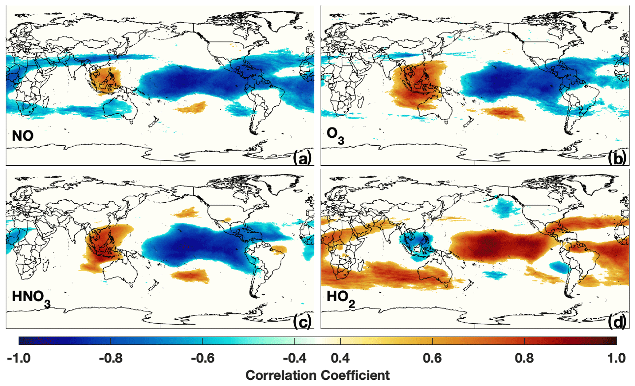
Figure 16Correlation of the indicated species with the MEI for the UFT level for DJF.
Regression analysis suggests that changes in NO are driving the relationship between OH and ENSO in the UFT in MERRA-2 GMI. The MEI–NO correlation exhibits a strong dipole pattern in the tropics (Fig. 16), with areas of positive correlation over southeast Asia and the maritime continent and a large area of anti-correlation over much of the Pacific. HO2 exhibits the opposite pattern, with increased concentrations over much of the Pacific during El Niño. This is consistent with the NO pattern, as decreased NO concentrations favor the partitioning of HOx (HOx = OH + HO2) towards HO2.
Similarities between NO and O3 correlation with the MEI in the UFT suggest similar mechanisms in controlling the spatial distribution of these species. The relationship between O3 and the MEI, shown in Fig. 16b, is similar to that found in Oman et al. (2013), using satellite data. They demonstrated that areas of increased O3 over Indonesia coincided with increased downward flow in the region associated with changes in the Walker circulation. Decreases in O3 over the Pacific coincided with increased upward motion, convectively lofting low O3 air throughout the column. Similarly, regions of anomalously low NO in the UFT during El Niño events are associated with regions of anomalous upward motion, suggesting that decreases in upper tropospheric NO results from the convective lofting of NOx-poor air from lower in the tropospheric column.
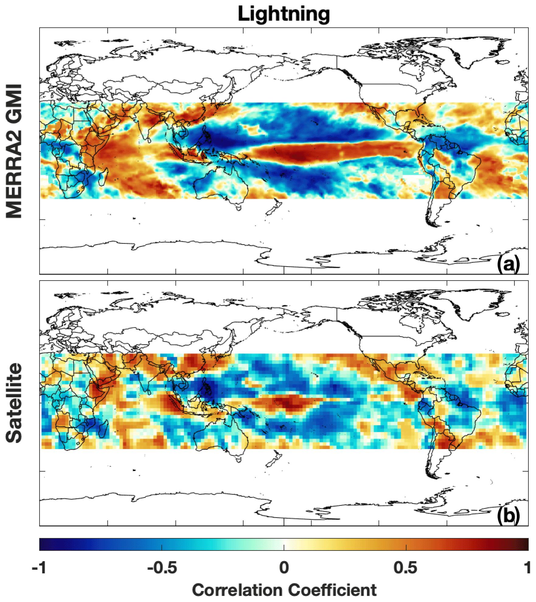
Figure 17The regression of lightning NO emissions at 300 hPa (a) and the lightning flash rate from the LIS/OTD time series (b) against the MEI. Lightning data are restricted to within 35∘ of the Equator because of the spatial coverage of the Tropical Rainfall Measuring Mission (TRMM) satellite on which LIS is located.
The anti-correlation between ENSO and NO also suggests that lightning emissions of NO over the tropical Pacific do not significantly increase OH production in the region during El Niño events. Lightning NO emissions in MERRA-2 GMI show a correlation pattern (Fig. 17) similar to that of H2O(v) (Fig. 9a), with increased lightning over the equatorial Pacific and decreased lightning poleward of this region during El Niño events. The correlation pattern from MERRA-2 GMI output agrees closely with flash rate data observed from the Lightning Imaging Sensor (LIS). The only region of significant difference between the satellite and MERRA-2 GMI is in the equatorial Pacific, where the region of positive correlation extends from Papua New Guinea to the South American coast in the simulation, but only about half that distance is covered in the satellite product.
This tripole correlation pattern between MEI and lightning, evident in both the satellite and model (Fig. 17) is in contrast to the relationship with NO (Fig. 16a) and other reactive nitrogen (NOy) species in the UFT. While the anti-correlation in NO is consistent with the changes in lightning NO emissions in some regions, in the equatorial Pacific band, NO decreases during El Niño events despite an increase in lightning NO emissions. This apparent discrepancy occurs because even though lightning NO increases by 100 % or more over the equatorial Pacific during El Niño events in the model, the absolute difference is orders of magnitude lower than the accompanying changes over land. We conclude that the resulting NO perturbations over the equatorial Pacific latitudes are dominated by mechanism other than the local lightning response, such as changes in the Walker circulation and the associated transport of air originating over the continents. This mechanism is supported by the similar regression pattern of longer-lived species, such as HNO3 (Fig. 16c) and PAN (not shown) and NO in the UFT, showing that transport of reactive nitrogen from other source regions, particularly lightning over South America, is likely reduced during El Niño events.
Our findings are broadly consistent with Turner et al. (2018), who found that increases in lightning NO emissions drive increases in OH during La Niña and, conversely, decreases in lightning NO emissions lead to OH decreases during El Niño. The results presented here suggest that, in addition to this influence of lightning locally, other mechanisms, such as atmospheric transport of NOy species, also likely contribute to the relationship between ENSO and OH in the equatorial Pacific.
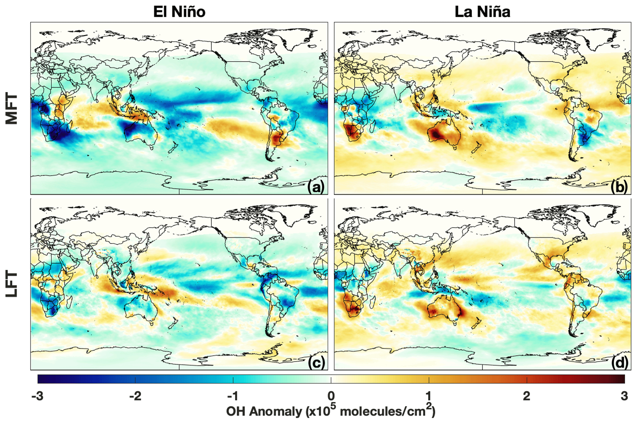
Figure 18Same as panels (a) and (b) of Fig. 7 except for the MFT and LFT.
5.4 Variability in the MFT and LFT
As in the UFT, ENSO is the dominant mode of variability in the MFT in DJF, with strong correlation between the MEI and the temporal component of the first EOF (r2 = 0.81) and the first EOF explaining 20.8 % of the total spatial variance. Likewise, the largest OH anomalies in the LFT during both El Niño and La Niña are centered over Australia and South Africa (Fig. 18), similar to patterns seen in the UFT. Unlike in the UFT, however, there is a large region extending from the coast of South America into the Pacific where OH concentration is positively correlated with ENSO. These changes are driven by the increase in H2O(v) and subsequent increased OH production from the H2O + O1D reaction.
ENSO-related changes in OH concentration in the LFT are smaller in magnitude than for the other atmospheric levels (Fig. 18), with maximum increases in OH during El Niño of the order of 1–1.5 × 10⁵ . The spatial extent of significant correlation between the MEI and OH concentration in the LFT is smaller than for the other atmospheric levels (Fig. 11), with the most prominent feature being an area of positive correlation near Indonesia. Consistent with the more limited impact, ENSO is correlated with the second EOF of OH concentration for the LFT (r2 = 0.55), explaining only 11.7 % of the total variability (Table 2).
It is likely that competing effects from the different drivers limit the interannual variability in OH in the LFT and MFT, explaining the smaller regions of correlation with ENSO. For these levels, no single OH production reaction clearly explains the relationship between ENSO and OH. In contrast to the PBL and UFT, where the relationship between the total OH production rate closely mirrored the production rates from the O1D + H2O and NO + HO2 reactions, respectively, there are no analogous relationships for the LFT and MFT. At these levels, no reaction clearly dominates total OH production (Fig. 6). Increases in H2O in the mid-troposphere, which would tend to increase OH, are offset by decreases in NO and O3. These competing effects likely explain why the absolute changes in OH are comparatively smaller in the LFT than in the other layers.
The comparatively smaller changes in LFT OH during El Niño events limit the effect of ENSO on the interannual variability of the CH4 lifetime. Global mean, mass-weighted tropospheric OH decreases by 2.2 % during El Niño events, corresponding to only a 1 % decrease in the CH4 lifetime. While changes in OH concentration are most pronounced in the UFT and PBL, the CH4 lifetime is mostly dictated by OH in the LFT due to the temperature dependence of the OH + CH4 reaction rate. This limited effect on CH4 lifetime highlights the importance of investigating the spatial OH variability as global mean metrics can obscure important year-to-year changes.

Figure 19The number of CCMI models that show a correlation between TCOH and ENSO over the period 1980 to 2010. Only regressions with an absolute value of r greater than 0.5 are included. All models have been regridded to a common horizontal grid. This regridding does not substantially alter the correlation patterns examined here. Grid boxes that also exhibit significant correlations between TCOH and ENSO for MERRA-2 GMI are indicated by the stippling.
5.5 Comparing simulated OH relationships with ENSO in MERRA-2 GMI with the CCMI models
To understand whether the relationship between OH and ENSO found in MERRA-2 GMI is robust, we examine model simulations from the CCMI. To compare the relationship between OH and ENSO among the different models, we performed the same regression analysis on TCOH for the four CCMI models considered here as for MERRA-2 GMI. Figure 19 shows the number of CCMI models that demonstrate a meaningful correlation between TCOH and the MEI, defined as the absolute value of r greater than 0.5, for each grid cell. To facilitate comparison, OH for each model has been regridded to the resolution of the model with the lowest horizontal resolution (2.81∘ longitude × 2.77∘ latitude). This regridding does not substantially alter the correlation patterns examined here.
In agreement with MERRA-2 GMI, TCOH varies with ENSO over a large fraction of the tropics in most of the CCMI models, with broadly similar spatial regression patterns for most models across all seasons, except for MAM (Fig. 19). In DJF, most models show strong correlation between ENSO and column OH over the central Pacific and south of the Aleutian Islands, with at least three CCMI models and MERRA-2 GMI showing correlation in each of these areas. This agreement highlights the relationship of OH with ENSO and with the PNA and Australian monsoon, as discussed in Sect. 6. Similar agreement among models was found for SON and JJA, although the spatial extent of the highly correlated region is much smaller for JJA. In SON, the expansion of the area of significant correlation over most of the Indian Ocean likely results from the strong relationship between the IOD and ENSO during this season. There is less agreement in MAM, with only one or two models showing strong correlation in most regions.
EOF analysis of the different CCMI models likewise suggests that, in DJF, ENSO is the dominant mode of TCOH variability. The spatial pattern of the first EOF of TCOH in DJF for the five models is shown in Fig. S10 in the Supplement, and the principal component time series, along with the time series of the MEI, is shown in Fig. S11 in the Supplement. MERRA-2 GMI, WACCM, and MRI show a strong correlation between the MEI and the first EOF (r2 > 0.64). For each of these models, ENSO is the cause of 29 %–48 % of the total spatial variance in TCOH. The correlation between the first EOF and the MEI for CHASER is weaker (r2 = 0.28), although the spatial component shows similarities to the other models. Correlation between the MEI and the EOFs for the UFT and MFT levels increases to 0.56 and 0.45, respectively, showing that ENSO is still important in controlling the interannual variability of CHASER, at least in the UFT. Similarly, EMAC has no correlation between the first EOF of TCOH and the MEI but does for the UFT layer (r2 = 0.64). This EOF explains 20 % of the total spatial variance for this level but has a substantially different spatial pattern than for the other models. While further work is needed to understand the cause of the relationship between OH and ENSO in the UFT in EMAC, results from MERRA-2 GMI suggest a role for changes in production via the NO + HO2 reaction.
The agreement among the majority of the models suggests that the relationship between ENSO and TCOH is robust. While SSTs and emissions are identical among the models, meteorology, chemical mechanisms, and parameterizations, such as that for lightning and convection, vary widely. Despite the differences in these chemical and dynamical drivers of OH, the spatial patterns of the ENSO TCOH relationship are similar for most models. While it is beyond the scope of this paper, determining the cause of intermodel differences in this relationship between OH and climate modes could further our understanding of the mechanisms driving interannual OH variability. Given the results from the MERRA-2 GMI analysis, investigating ENSO-related changes in UFT NO, both from lightning and transport, could provide insight into these intermodel differences. Furthermore, Nicely et al. (2020) showed that J(O1D) was the largest driver in differences in the methane lifetime in the CCMI models, suggesting the potential importance of this variable in intermodel differences in the OH–ENSO relationship in the PBL and lower troposphere.
We now investigate the relationship between OH and the NH modes of variability, monsoons, and the IOD. In Sect. 6.1, we evaluate the relationships in MERRA-2 GMI, demonstrating that these other climate features exert a much more spatially limited influence on OH as compared to ENSO (Fig. 5). Despite the comparatively limited extent of influence, each of these modes of variability can strongly influence the atmospheric oxidative capacity on the local scale. In Sect. 6.2, we compare the results from MERRA-2 GMI to CCMI simulations, demonstrating that the relationship between OH and the IOD and NH modes is robust among models, while the relationship between monsoons and OH is primarily limited to MERRA-2 GMI.
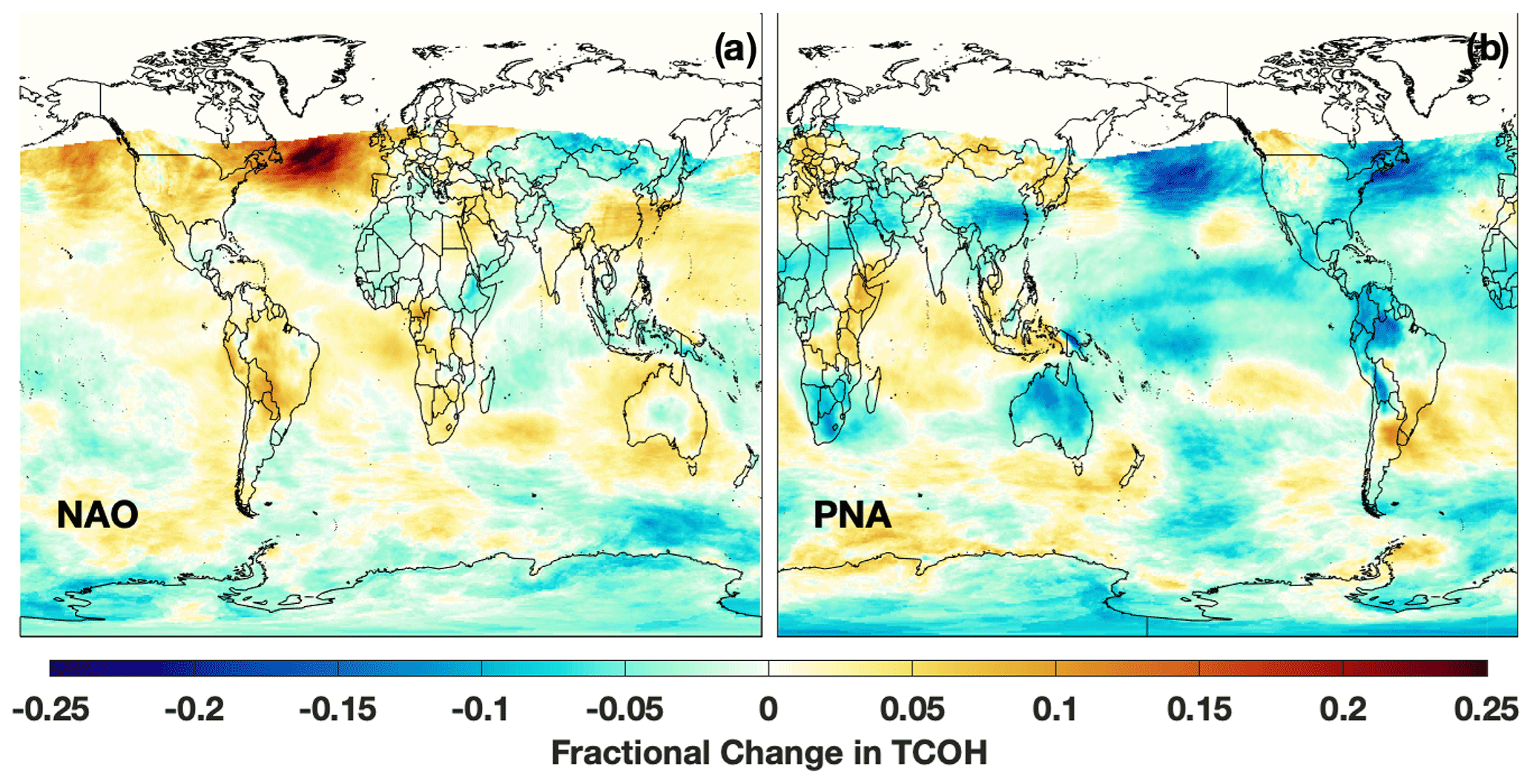
Figure 20Fractional change in TCOH for positive phases of the NAO (a) and PNA (b), defined as having an index greater than 0.4, as compared to neutral events (index between −0.4 and 0.4). Note that, for emphasis, the x axis is shifted in panel (b) to center the map over the Pacific Ocean.
6.1 Simulated OH and the NH climate modes, monsoons, and the IOD in MERRA-2 GMI
Northern hemispheric modes of variability are strongly correlated (r > 0.5) with OH over ∼ 10 % of the globe during DJF but have a comparatively smaller effect on global OH than ENSO. During the positive phases of the NAO, defined as the index being greater than 0.4, TCOH increases by up to 25 % in the northern Atlantic. Similarly, during the positive phase of the PNA, TCOH decreases by 10 %–20 % in the northern Pacific (Fig. 20). Because OH production is almost an order of magnitude lower in the NH mid-latitudes than in the tropics (Fig. 6c), however, the resultant decrease in global mean mass-weighted OH (e.g., Lawrence et al., 2001) during the positive phase of the NAO is only 0.77 %, as compared to decreases of 2.2 % during an El Niño event. Similar results are found for the other NH modes.
The effects of the monsoons on OH interannual variability are much more localized than for ENSO and vary markedly among the different monsoons (Fig. S12 in the Supplement). For example, Fig. S13a in the Supplement shows the partial correlation coefficient (e.g., Sekiya and Sudo, 2012) of TCOH with the Australian monsoon, taking into account the correlation of the Australian monsoon index with the MEI, which has an r2 of 0.65 for DJF. Correlation is almost exclusively restricted to areas near the Australian continent. In this region, however, monsoons with an index in the 75th percentile or higher result in TCOH that is 15 %–20 % (up to 7 × 10¹¹ ) higher than for monsoons with an index between the 25th and 75th percentile (Fig. S14 in the Supplement). These increases in OH column for the strongest monsoons are larger in magnitude than typical changes associated with ENSO, although they are limited to a smaller region, suggesting that the Australian monsoon can significantly perturb the local atmospheric oxidative capacity.
In contrast, despite its larger scale, the Asian monsoon only shows a correlation with TCOH over a small portion of the subcontinent (Fig. S12b and d). Correlations outside of the subcontinent region result from the correlation between the Asian monsoon and ENSO. Interestingly, this correlation is only present during MAM and SON and not during JJA when the Asian monsoon is at full strength. Lelieveld et al. (2018) have shown, using in situ observations, that upper tropospheric OH is increased during the Asian monsoon. The lack of correlation demonstrated here suggests that the model is not accurately capturing the chemical variability within the monsoon anticyclone. The correlation with the monsoon index for MAM and SON could result from interannual variability at the start and end of the monsoon. Since these seasons are at the fringe of the monsoon, yearly variations in the start and end date would lead to larger variability than that seen during JJA when the monsoon is active every year.
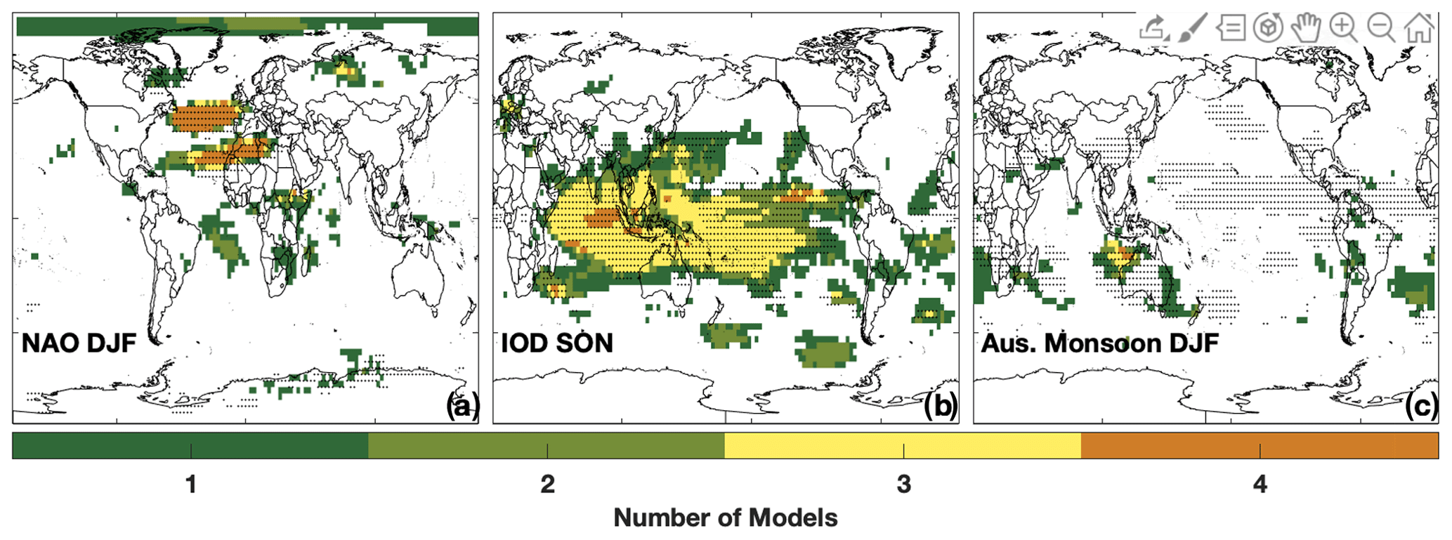
Figure 21Same as Fig. 19 except for the NAO (a), the IOD (b), and the Australian Monsoon (c). The NAO and Australian monsoon are shown for DJF and the IOD for SON.
The IOD also shows a strong relationship with OH, although, due to its annual cycle, the relationship is only present during SON (Fig. 5d). Taking into account the correlation between ENSO and the IOD (r2 = 0.30), the partial correlation between the Dipole Mode Index (DMI) and TCOH becomes mostly restricted to the western Indian Ocean (Fig. S13b), where TCOH is anticorrelated with the DMI, resulting in decreases in TCOH of the order of 10 % (about 1.5 × 10¹¹ ). During the positive phase of the IOD, the Indian Ocean basin exhibits a Walker-type circulation with anomalous surface easterly winds and increased convection in the region that exhibits anticorrelation between OH and the DMI. This region is also characterized by an anticorrelation between the DMI and OH production from the NO + HO2 reaction, despite a positive correlation with lightning NO emissions analogous to the relationship between NO and ENSO in the equatorial Pacific. This suggests that the anticorrelation between TCOH and the DMI in the eastern Indian Ocean is being driven by changes in NO transport from this Walker-type circulation. More work is needed, however, to prove this relationship, as the correlations between OH production from the NO + HO2 reaction and the DMI do not meet our stated statistical significance criteria.
6.2 Simulated OH and the NH climate modes, monsoons, and the IOD in the CCMI models
The MERRA-2 GMI and the CCMI simulations exhibit nearly identical spatial relationships between TCOH and the NH climate modes and the IOD, demonstrating that these relationships are robust among multiple models. For example, all five models show two broad regions of correlation between the NAO and TCOH, corresponding to the dipole pattern of the NAO (Fig. 21a). Similar agreement is found for the other NH modes (Fig. S15 in the Supplement). Likewise, most models show the same pattern of correlation between the IOD and TCOH (Fig. 21b), consistent with their agreement for ENSO, since the two modes are closely related.
In contrast to the other modes of variability, the relationship between TCOH and the different monsoons varies widely among the models. Agreement is highest for the Australian monsoon (Fig. 21c), where most models see correlation off the northwestern coast of the continent. For the other monsoons considered here, there is no consistent relationship with OH, with MERRA-2 GMI being the only model showing correlations with most monsoons (Fig. S16 in the Supplement). While models and observations have shown the monsoons can change OH abundance, particularly in the UFT (Lelieveld et al., 2018), the lack of correlation among the models suggests either that those changes are not highly variable from year to year or that not all models capture the mechanisms behind monsoon influence on OH, such as convective lofting of OH precursors.
Because of limited in situ observations and intermodel differences, there is significant uncertainty in the processes driving interannual OH variability, despite its importance in controlling the removal of many atmospheric trace gases. Here, we have explored the relationship between OH and multiple modes of climate variability, including ENSO, the IOD, NH modes of variability, and monsoons, in order to understand how these large-scale dynamical features influence OH through control of its dynamical and photochemical drivers.
Using output from the MERRA-2 GMI simulation, we have shown that during DJF, when considered together, these climate features can explain a portion of OH variability over approximately 40 % of the troposphere by mass. ENSO is the dominant mode of variability in all seasons except for JJA and can explain 20 %–30 % of the spatial variance in TCOH and results in an average decrease in the global, mass weighted OH of 2.2 % during El Niño events. Effects from the other modes of variability considered here are more limited in spatial scale but can strongly alter the atmospheric oxidative capacity on the local scale. For example, changes in TCOH for the NAO, IOD, and Australian monsoon can reach 0.5, 1.5, and 7 × 10¹¹ , respectively, compared to 2 × 10¹¹ for ENSO.
Changes in OH with ENSO are driven by different processes in the upper and lower troposphere. In the PBL, where OH production is dominated by the reaction of O1D with water, changes in the distribution of these species lead to a positive correlation between OH and ENSO. Increases in H2O(v) during El Niño are associated with increased convection and warmer SSTs, while increases in O1D result from increased horizontal advection of O3 in the western Pacific and increased photolysis rates resulting from reduced stratospheric O3 in the eastern Pacific. In the upper troposphere, NO controls the OH abundance over the tropical Pacific. In much of the region, decreases in lightning NO production correspond to decreases in total NO and, thus, OH. In the equatorial region, however, increases in lightning NO production are offset by other processes, potentially including transport due to changes in the Walker circulation. Further work is needed to determine the relative importance of these two factors in controlling OH in the region during El Niño and La Niña events.
Absolute changes in OH concentration during El Niño and La Niña events in the LFT and, to a lesser extent, the MFT were limited by competing effects from changes in the O1D + H2O and NO + HO2 reactions. As a result, ENSO only explains 11.7 % of the variability in the LFT and is associated with the second EOF. Because OH variability in the LFT drives variability in the CH4 lifetime, which showed limited response to ENSO variability, further research is warranted to understand the dominant mode of OH variability at this level, including any impacts in emissions trends, which appear to be the dominant mode of variability in the PBL.
The relationship between the individual climate modes seen in MERRA-2 GMI is also seen in the majority of the CCMI models, suggesting that the relationship between the modes and OH is robust. A total of four of the five models examined here show similar relationships between ENSO and TCOH for all seasons except MAM, and three of those models suggest that ENSO is the dominant mode of OH variability in DJF, responsible for between 30 % and 50 % of total spatial variance. Similar agreement is found for the NH modes of variability and the IOD, while there is little agreement among models between the relationship of the individual monsoons and OH.
Despite the agreement among models in the importance of the driving factors of OH variability, there is still a lack of observations demonstrating that the models are accurate. We have shown here that satellite observations of H2O, CO, lightning flashes, and, to a lesser extent, NO2 are able to capture the respective variability in each variable and the relationship with ENSO while being in excellent agreement with the model simulation. While further understanding of the relationship between these species and ENSO is needed, the results presented here suggest that combining the observations of OH drivers and the various climate modes could lead to additional methods to constrain OH from space.
All output from MERRA-2 GMI is publicly available at https://acd-ext.gsfc.nasa.gov/Projects/GEOSCCM/MERRA2GMI/ (NASA Goddard Space Flight Center, 2021). Output from the EMAC, MRI, and CHASER models is available from the Centre for Environmental Data Analysis at http://data.ceda.ac.uk/badc/wcrp-ccmi/data/CCMI-1/output (CEDA Archive, 2021). Output from WACCM is available at http://www.earthsystemgrid.org (Climate Data Gateway at NCAR, 2021). Satellite data are available at https://disc.gsfc.nasa.gov (GES DISC, 2021). Data from the ATom campaign are located at https://espoarchive.nasa.gov/archive/browse/atom (Science team of the NASA Atmospheric Tomography Mission, 2021).
The supplement related to this article is available online at: https://doi.org/10.5194/acp-21-6481-2021-supplement.
DCA performed the analysis and wrote the paper. BND developed the initial idea for the work and helped write the paper. AMF, CBB, MBFC, JMN, and GMW helped develop ideas for the paper through discussions in biweekly calls and provided feedback on the paper.
The authors declare that they have no conflict of interest.
We acknowledge the modeling groups for making their simulations available for this analysis, the joint WCRP SPARC/IGAC Chemistry–Climate Model Initiative (CCMI) for organizing and coordinating the model data analysis activity, and the British Atmospheric Data Centre (BADC) for collecting and archiving the CCMI model output.
This research has been supported in part by the NASA Aura ACMAP program (grant no. 16-ACMAP16-0027).
This paper was edited by Christopher Cantrell and reviewed by two anonymous referees.
Allen, D., Pickering, K., Duncan, B., and Damon, M.: Impact of lightning NO emissions on North American photochemistry as determined using the Global Modeling Initiative (GMI) model, J. Geophys. Res., 115, D22301, https://doi.org/10.1029/2010jd014062, 2010.
Anderson, D. C., Nicely, J. M., Wolfe, G. M., Hanisco, T. F., Salawitch, R. J., Canty, T. P., Dickerson, R. R., Apel, E. C., Baidar, S., Bannan, T. J., Blake, N. J., Chen, D. X., Dix, B., Fernandez, R. P., Hall, S. R., Hornbrook, R. S., Huey, L. G., Josse, B., Jockel, P., Kinnison, D. E., Koenig, T. K., Le Breton, M., Marecal, V., Morgenstern, O., Oman, L. D., Pan, L. L., Percival, C., Plummer, D., Revell, L. E., Rozanov, E., Saiz-Lopez, A., Stenke, A., Sudo, K., Tilmes, S., Ullmann, K., Volkamer, R., Weinheimer, A. J., and Zeng, G.: Formaldehyde in the Tropical Western Pacific: Chemical Sources and Sinks, Convective Transport, and Representation in CAM-Chem and the CCMI Models, J. Geophys. Res.-Atmos., 122, 11201–11226, https://doi.org/10.1002/2016jd026121, 2017.
Barnston, A. G. and Livezey, R. E.: Classification, Seasonality and Persistence of Low-Frequency Atmospheric Circulation Patterns, Mon. Weather Rev., 115, 1083–1126, https://doi.org/10.1175/1520-0493(1987)115<1083:CSAPOL>2.0.CO;2, 1987.
Borlace, S., Santoso, A., Cai, W., and Collins, M.: Extreme swings of the South Pacific Convergence Zone and the different types of El Niño events, Geophys. Res. Lett., 41, 4695–4703, https://doi.org/10.1002/2014gl060551, 2014.
Bosilovich, M. G., Akella, S., Coy, L., Cullather, R., Draper, C., Gelaro, R., Kovach, R., Liu, Q., Molod, A., Norris, P., Wargan, K., Chao, W., Reichle, R., Takacs, L., Vikhliaev, Y., Bloom, S., Collow, A., Firth, S., Labow, G., Partyka, G., Pawson, S., Reale, O., Schubert, S. D., and Suarez, M.: MERRA-2: Initial Evaluation of the Climate, Technical Report Series on Global Modeling and Data Assimilation, NASA Goddard Space Flight Center, Greenbelt, MD, 43, 2015.
Brune, W. H., Miller, D. O., Thames, A. B., Allen, H. M., Apel, E. C., Blake, D. R., Bui, T. P., Commane, R., Crounse, J. D., Daube, B. C., Diskin, G. S., DiGangi, J. P., Elkins, J. W., Hall, S. R., Hanisco, T. F., Hannun, R. A., Hintsa, E. J., Hornbrook, R. S., Kim, M. J., McKain, K., Moore, F. L., Neuman, J. A., Nicely, J. M., Peischl, J., Ryerson, T. B., St. Clair, J. M., Sweeney, C., Teng, A. P., Thompson, C., Ullmann, K., Veres, P. R., Wennberg, P. O., and Wolfe, G. M.: Exploring Oxidation in the Remote Free Troposphere: Insights From Atmospheric Tomography (ATom), J. Geophys. Res.-Atmos., 125, e2019JD031685, https://doi.org/10.1029/2019jd031685, 2020.
Buchholz, R. R., Hammerling, D., Worden, H. M., Deeter, M. N., Emmons, L. K., Edwards, D. P., and Monks, S. A.: Links Between Carbon Monoxide and Climate Indices for the Southern Hemisphere and Tropical Fire Regions, J. Geophys. Res.-Atmos., 123, 9786–9800, https://doi.org/10.1029/2018jd028438, 2018.
Cecil, D. J., Buechler, D. E., and Blakeslee, R. J.: Gridded lightning climatology from TRMM-LIS and OTD: Dataset description, Atmos. Res., 135, 404–414, https://doi.org/10.1016/j.atmosres.2012.06.028, 2014.
CEDA Archive: CCMI-1 Data Archive, available at: http://data.ceda.ac.uk/badc/wcrp-ccmi/data/CCMI-1/output, last access: 21 April 2021.
Climate Data Gateway at NCAR: Climate Data at the National Center for Atmospheric Research, available at: https://www.earthsystemgrid.org/, last access: 21 April 2021.
Creilson, J. K., Fishman, J., and Wozniak, A. E.: Intercontinental transport of tropospheric ozone: a study of its seasonal variability across the North Atlantic utilizing tropospheric ozone residuals and its relationship to the North Atlantic Oscillation, Atmos. Chem. Phys., 3, 2053–2066, https://doi.org/10.5194/acp-3-2053-2003, 2003.
Deeter, M. N., Edwards, D. P., Francis, G. L., Gille, J. C., Mao, D., Martínez-Alonso, S., Worden, H. M., Ziskin, D., and Andreae, M. O.: Radiance-based retrieval bias mitigation for the MOPITT instrument: the version 8 product, Atmos. Meas. Tech., 12, 4561–4580, https://doi.org/10.5194/amt-12-4561-2019, 2019.
Dhomse, S. S., Kinnison, D., Chipperfield, M. P., Salawitch, R. J., Cionni, I., Hegglin, M. I., Abraham, N. L., Akiyoshi, H., Archibald, A. T., Bednarz, E. M., Bekki, S., Braesicke, P., Butchart, N., Dameris, M., Deushi, M., Frith, S., Hardiman, S. C., Hassler, B., Horowitz, L. W., Hu, R.-M., Jöckel, P., Josse, B., Kirner, O., Kremser, S., Langematz, U., Lewis, J., Marchand, M., Lin, M., Mancini, E., Marécal, V., Michou, M., Morgenstern, O., O'Connor, F. M., Oman, L., Pitari, G., Plummer, D. A., Pyle, J. A., Revell, L. E., Rozanov, E., Schofield, R., Stenke, A., Stone, K., Sudo, K., Tilmes, S., Visioni, D., Yamashita, Y., and Zeng, G.: Estimates of ozone return dates from Chemistry-Climate Model Initiative simulations, Atmos. Chem. Phys., 18, 8409–8438, https://doi.org/10.5194/acp-18-8409-2018, 2018.
Dlugokencky, E. J., Steele, L. P., Lang, P. M., and Masarie, K. A.: The growth rate and distribution of atmospheric methane, J. Geophys. Res.-Atmos., 99, 17021–17043, https://doi.org/10.1029/94JD01245, 1994.
Duncan, B. N., Bey, I., Chin, M., Mickley, L. J., Fairlie, T. D., Martin, R. V., Matsueda, H.: Indonesian wildfires of 1997: Impact on tropospheric chemistry, J. Geophys. Res., 108, JD003195, https://doi.org/10.1029/2002jd003195, 2003a.
Duncan, B. N., Martin, R. V., and Staudt, A. C.: Interannual and seasonal variability of biomass burning emissions constrained by satellite observations, J. Geophys. Res., 108, D002378, https://doi.org/10.1029/2002jd002378, 2003b.
Duncan, B. N. and Bey, I.: A modeling study of the export pathways of pollution from Europe: Seasonal and interannual variations (1987–1997), J. Geophys. Res., 109, D22301, https://doi.org/10.1029/2003jd004079, 2004.
Duncan, B. N., Logan, J. A., Bey, I., Megretskaia, I. A., Yantosca, R. M., Novelli, P. C., Jones, N. B., and Rinsland, C. P.: Global budget of CO, 1988–1997: Source estimates and validation with a global model, J. Geophys. Res., 112, D22301, https://doi.org/10.1029/2007jd008459, 2007.
GES DISC: Earth Science Data at NASA, available at: https://disc.gsfc.nasa.gov, last access: 21 April 2021.
Fisher, J. A., Jacob, D. J., Purdy, M. T., Kopacz, M., Le Sager, P., Carouge, C., Holmes, C. D., Yantosca, R. M., Batchelor, R. L., Strong, K., Diskin, G. S., Fuelberg, H. E., Holloway, J. S., Hyer, E. J., McMillan, W. W., Warner, J., Streets, D. G., Zhang, Q., Wang, Y., and Wu, S.: Source attribution and interannual variability of Arctic pollution in spring constrained by aircraft (ARCTAS, ARCPAC) and satellite (AIRS) observations of carbon monoxide, Atmos. Chem. Phys., 10, 977–996, https://doi.org/10.5194/acp-10-977-2010, 2010.
Gelaro, R., McCarty, W., Suarez, M. J., Todling, R., Molod, A., Takacs, L., Randles, C., Darmenov, A., Bosilovich, M. G., Reichle, R., Wargan, K., Coy, L., Cullather, R., Draper, C., Akella, S., Buchard, V., Conaty, A., da Silva, A., Gu, W., Kim, G. K., Koster, R., Lucchesi, R., Merkova, D., Nielsen, J. E., Partyka, G., Pawson, S., Putman, W., Rienecker, M., Schubert, S. D., Sienkiewicz, M., and Zhao, B.: The Modern-Era Retrospective Analysis for Research and Applications, Version 2 (MERRA-2), J. Climate, 30, 5419–5454, https://doi.org/10.1175/JCLI-D-16-0758.1, 2017.
Giglio, L., Randerson, J. T., and van der Werf, G. R.: Analysis of daily, monthly, and annual burned area using the fourth-generation global fire emissions database (GFED4), J. Geophys. Res.-Biogeo., 118, 317–328, https://doi.org/10.1002/jgrg.20042, 2013.
Granier, C., Bessagnet, B., Bond, T., D'Angiola, A., Denier van der Gon, H., Frost, G. J., Heil, A., Kaiser, J. W., Kinne, S., Klimont, Z., Kloster, S., Lamarque, J.-F., Liousse, C., Masui, T., Meleux, F., Mieville, A., Ohara, T., Raut, J.-C., Riahi, K., Schultz, M. G., Smith, S. J., Thompson, A., van Aardenne, J., van der Werf, G. R., and van Vuuren, D. P.: Evolution of anthropogenic and biomass burning emissions of air pollutants at global and regional scales during the 1980–2010 period, Climatic Change, 109, 163–190, https://doi.org/10.1007/s10584-011-0154-1, 2011.
Guenther, A., Baugh, B., Brasseur, G., Greenberg, J., Harley, P., Klinger, L., Serça, D., and Vierling, L.: Isoprene emission estimates and uncertainties for the central African EXPRESSO study domain, J. Geophys. Res.-Atmos., 104, 30625–30639, https://doi.org/10.1029/1999JD900391, 1999.
Guenther, A., Geron, C., Pierce, T., Lamb, B., Harley, P., and Fall, R.: Natural emissions of non-methane volatile organic compounds, carbon monoxide, and oxides of nitrogen from North America, Atmos. Environ., 34, 2205–2230, https://doi.org/10.1016/S1352-2310(99)00465-3, 2000.
Jöckel, P., Tost, H., Pozzer, A., Kunze, M., Kirner, O., Brenninkmeijer, C. A. M., Brinkop, S., Cai, D. S., Dyroff, C., Eckstein, J., Frank, F., Garny, H., Gottschaldt, K.-D., Graf, P., Grewe, V., Kerkweg, A., Kern, B., Matthes, S., Mertens, M., Meul, S., Neumaier, M., Nützel, M., Oberländer-Hayn, S., Ruhnke, R., Runde, T., Sander, R., Scharffe, D., and Zahn, A.: Earth System Chemistry integrated Modelling (ESCiMo) with the Modular Earth Submodel System (MESSy) version 2.51, Geosci. Model Dev., 9, 1153–1200, https://doi.org/10.5194/gmd-9-1153-2016, 2016.
Lamarque, J.-F., Bond, T. C., Eyring, V., Granier, C., Heil, A., Klimont, Z., Lee, D., Liousse, C., Mieville, A., Owen, B., Schultz, M. G., Shindell, D., Smith, S. J., Stehfest, E., Van Aardenne, J., Cooper, O. R., Kainuma, M., Mahowald, N., McConnell, J. R., Naik, V., Riahi, K., and van Vuuren, D. P.: Historical (1850–2000) gridded anthropogenic and biomass burning emissions of reactive gases and aerosols: methodology and application, Atmos. Chem. Phys., 10, 7017–7039, https://doi.org/10.5194/acp-10-7017-2010, 2010.
Lamsal, L. N., Krotkov, N. A., Vasilkov, A., Marchenko, S., Qin, W., Yang, E.-S., Fasnacht, Z., Joiner, J., Choi, S., Haffner, D., Swartz, W. H., Fisher, B., and Bucsela, E.: Ozone Monitoring Instrument (OMI) Aura nitrogen dioxide standard product version 4.0 with improved surface and cloud treatments, Atmos. Meas. Tech., 14, 455–479, https://doi.org/10.5194/amt-14-455-2021, 2021.
Lawrence, M. G., Jöckel, P., and von Kuhlmann, R.: What does the global mean OH concentration tell us?, Atmos. Chem. Phys., 1, 37–49, https://doi.org/10.5194/acp-1-37-2001, 2001.
Lelieveld, J., Bourtsoukidis, E., Bruhl, C., Fischer, H., Fuchs, H., Harder, H., Hofzumahaus, A., Holland, F., Marno, D., Neumaier, M., Pozzer, A., Schlager, H., Williams, J., Zahn, A., and Ziereis, H.: The South Asian monsoon-pollution pump and purifier, Science, 361, 270–273, https://doi.org/10.1126/science.aar2501, 2018.
Li, Q., Jacob, D. J., Bey, I., Palmer, P. I., Duncan, B. N., Field, B. D., Martin, R. V., Fiore, A. M., Yantosca, R. M., Parrish, D. D., Simmonds, P. G., and Oltmans, S. J.: Transatlantic transport of pollution and its effects on surface ozone in Europe and North America, J. Geophys. Res.-Atmos., 107, ACH 4-1–ACH 4-21, https://doi.org/10.1029/2001JD001422, 2002.
Mao, J., Ren, X., Brune, W. H., Olson, J. R., Crawford, J. H., Fried, A., Huey, L. G., Cohen, R. C., Heikes, B., Singh, H. B., Blake, D. R., Sachse, G. W., Diskin, G. S., Hall, S. R., and Shetter, R. E.: Airborne measurement of OH reactivity during INTEX-B, Atmos. Chem. Phys., 9, 163–173, https://doi.org/10.5194/acp-9-163-2009, 2009.
Melton, J. R., Wania, R., Hodson, E. L., Poulter, B., Ringeval, B., Spahni, R., Bohn, T., Avis, C. A., Beerling, D. J., Chen, G., Eliseev, A. V., Denisov, S. N., Hopcroft, P. O., Lettenmaier, D. P., Riley, W. J., Singarayer, J. S., Subin, Z. M., Tian, H., Zürcher, S., Brovkin, V., van Bodegom, P. M., Kleinen, T., Yu, Z. C., and Kaplan, J. O.: Present state of global wetland extent and wetland methane modelling: conclusions from a model inter-comparison project (WETCHIMP), Biogeosciences, 10, 753–788, https://doi.org/10.5194/bg-10-753-2013, 2013.
Morgenstern, O., Hegglin, M. I., Rozanov, E., O'Connor, F. M., Abraham, N. L., Akiyoshi, H., Archibald, A. T., Bekki, S., Butchart, N., Chipperfield, M. P., Deushi, M., Dhomse, S. S., Garcia, R. R., Hardiman, S. C., Horowitz, L. W., Jöckel, P., Josse, B., Kinnison, D., Lin, M., Mancini, E., Manyin, M. E., Marchand, M., Marécal, V., Michou, M., Oman, L. D., Pitari, G., Plummer, D. A., Revell, L. E., Saint-Martin, D., Schofield, R., Stenke, A., Stone, K., Sudo, K., Tanaka, T. Y., Tilmes, S., Yamashita, Y., Yoshida, K., and Zeng, G.: Review of the global models used within phase 1 of the Chemistry–Climate Model Initiative (CCMI), Geosci. Model Dev., 10, 639–671, https://doi.org/10.5194/gmd-10-639-2017, 2017.
Murray, L. T., Logan, J. A., and Jacob, D. J.: Interannual variability in tropical tropospheric ozone and OH: The role of lightning, J. Geophys. Res.-Atmos., 118, 11468–11480, https://doi.org/10.1002/jgrd.50857, 2013.
Murray, L. T., Mickley, L. J., Kaplan, J. O., Sofen, E. D., Pfeiffer, M., and Alexander, B.: Factors controlling variability in the oxidative capacity of the troposphere since the Last Glacial Maximum, Atmos. Chem. Phys., 14, 3589–3622, https://doi.org/10.5194/acp-14-3589-2014, 2014.
Myers, D. S. and Waliser, D. E.: Three-Dimensional Water Vapor and Cloud Variations Associated with the Madden–Julian Oscillation during Northern Hemisphere Winter, J. Climate, 16, 929–950, https://doi.org/10.1175/1520-0442(2003)016<0929:TDWVAC>2.0.CO;2, 2003.
Naik, V., Voulgarakis, A., Fiore, A. M., Horowitz, L. W., Lamarque, J.-F., Lin, M., Prather, M. J., Young, P. J., Bergmann, D., Cameron-Smith, P. J., Cionni, I., Collins, W. J., Dalsøren, S. B., Doherty, R., Eyring, V., Faluvegi, G., Folberth, G. A., Josse, B., Lee, Y. H., MacKenzie, I. A., Nagashima, T., van Noije, T. P. C., Plummer, D. A., Righi, M., Rumbold, S. T., Skeie, R., Shindell, D. T., Stevenson, D. S., Strode, S., Sudo, K., Szopa, S., and Zeng, G.: Preindustrial to present-day changes in tropospheric hydroxyl radical and methane lifetime from the Atmospheric Chemistry and Climate Model Intercomparison Project (ACCMIP), Atmos. Chem. Phys., 13, 5277–5298, https://doi.org/10.5194/acp-13-5277-2013, 2013.
NASA Goddard Space Flight Center: MERRA2 GMI, available at: https://acd-ext.gsfc.nasa.gov/Projects/GEOSCCM/MERRA2GMI, last access: 21 April 2021.
Nicely, J. M., Salawitch, R. J., Canty, T., Anderson, D. C., Arnold, S. R., Chipperfield, M. P., Emmons, L. K., Flemming, J., Huijnen, V., Kinnison, D. E., Lamarque, J.-F., Mao, J., Monks, S. A., Steenrod, S. D., Tilmes, S., and Turquety, S.: Quantifying the causes of differences in tropospheric OH within global models, J. Geophys. Res.-Atmos., 122, D026239, https://doi.org/10.1002/2016JD026239, 2017.
Nicely, J. M., Duncan, B. N., Hanisco, T. F., Wolfe, G. M., Salawitch, R. J., Deushi, M., Haslerud, A. S., Jöckel, P., Josse, B., Kinnison, D. E., Klekociuk, A., Manyin, M. E., Marécal, V., Morgenstern, O., Murray, L. T., Myhre, G., Oman, L. D., Pitari, G., Pozzer, A., Quaglia, I., Revell, L. E., Rozanov, E., Stenke, A., Stone, K., Strahan, S., Tilmes, S., Tost, H., Westervelt, D. M., and Zeng, G.: A machine learning examination of hydroxyl radical differences among model simulations for CCMI-1, Atmos. Chem. Phys., 20, 1341–1361, https://doi.org/10.5194/acp-20-1341-2020, 2020.
Nisbet, E. G., Dlugokencky, E. J., Manning, M. R., Lowry, D., Fisher, R. E., France, J. L., Michel, S. E., Miller, J. B., White, J. W. C., Vaughn, B., Bousquet, P., Pyle, J. A., Warwick, N. J., Cain, M., Brownlow, R., Zazzeri, G., Lanoisellé, M., Manning, A. C., Gloor, E., Worthy, D. E. J., Brunke, E. G., Labuschagne, C., Wolff, E. W., and Ganesan, A. L.: Rising atmospheric methane: 2007–2014 growth and isotopic shift, Global Biogeochem. Cy., 30, 1356–1370, https://doi.org/10.1002/2016gb005406, 2016.
Oman, L. D., Ziemke, J. R., Douglass, A. R., Waugh, D. W., Lang, C., Rodriguez, J. M., and Nielsen, J. E.: The response of tropical tropospheric ozone to ENSO, Geophys. Res. Lett., 38, https://doi.org/10.1029/2011gl047865, 2011.
Oman, L. D., Douglass, A. R., Ziemke, J. R., Rodriguez, J. M., Waugh, D. W., and Nielsen, J. E.: The ozone response to ENSO in Aura satellite measurements and a chemistry–climate simulation, J. Geophys. Res.-Atmos., 118, 965–976, https://doi.org/10.1029/2012jd018546, 2013.
Orbe, C., Oman, L. D., Strahan, S. E., Waugh, D. W., Pawson, S., Takacs, L. L., and Molod, A. M.: Large-Scale Atmospheric Transport in GEOS Replay Simulations, J. Adv. Model. Earth Sy., 9, 2545–2560, https://doi.org/10.1002/2017ms001053, 2017.
Orbe, C., Plummer, D. A., Waugh, D. W., Yang, H., Jöckel, P., Kinnison, D. E., Josse, B., Marecal, V., Deushi, M., Abraham, N. L., Archibald, A. T., Chipperfield, M. P., Dhomse, S., Feng, W., and Bekki, S.: Description and Evaluation of the specified-dynamics experiment in the Chemistry-Climate Model Initiative , Atmos. Chem. Phys., 20, 3809–3840, https://doi.org/10.5194/acp-20-3809-2020, 2020.
Pan, L. L., Randel, W. J., Gary, B. L., Mahoney, M. J., and Hintsa, E. J.: Definitions and sharpness of the extratropical tropopause: A trace gas perspective, J. Geophys. Res.-Atmos., 109, https://doi.org/10.1029/2004JD004982, 2004.
Prather, M. J. and Holmes, C. D.: Overexplaining or underexplaining methane's role in climate change, P. Natl. Acad. Sci. USA, 114, 5324–5326, https://doi.org/10.1073/pnas.1704884114, 2017.
Prinn, R. G., Huang, J., Weiss, R. F., Cunnold, D. M., Fraser, P. J., Simmonds, P. G., McCulloch, A., Harth, C., Salameh, P., O'Do, Wang, R. H. J., Porter, L., and Miller, B. R.: Evidence for Substantial Variations of Atmospheric Hydroxyl Radicals in the Past Two Decades, Science, 292, 1882–1888, https://doi.org/10.1126/science.1058673, 2001.
Randel, W. J., Garcia, R. R., Calvo, N., and Marsh, D.: ENSO influence on zonal mean temperature and ozone in the tropical lower stratosphere, Geophys. Res. Lett., 36, https://doi.org/10.1029/2009GL039343, 2009.
Revell, L. E., Stenke, A., Tummon, F., Feinberg, A., Rozanov, E., Peter, T., Abraham, N. L., Akiyoshi, H., Archibald, A. T., Butchart, N., Deushi, M., Jöckel, P., Kinnison, D., Michou, M., Morgenstern, O., O'Connor, F. M., Oman, L. D., Pitari, G., Plummer, D. A., Schofield, R., Stone, K., Tilmes, S., Visioni, D., Yamashita, Y., and Zeng, G.: Tropospheric ozone in CCMI models and Gaussian process emulation to understand biases in the SOCOLv3 chemistry–climate model, Atmos. Chem. Phys., 18, 16155–16172, https://doi.org/10.5194/acp-18-16155-2018, 2018.
Rigby, M., Montzka, S. A., Prinn, R. G., White, J. W. C., Young, D., O'Doherty, S., Lunt, M. F., Ganesan, A. L., Manning, A. J., Simmonds, P. G., Salameh, P. K., Harth, C. M., Muhle, J., Weiss, R. F., Fraser, P. J., Steele, L. P., Krummel, P. B., McCulloch, A., and Park, S.: Role of atmospheric oxidation in recent methane growth, P. Natl. Acad. Sci. USA, 114, 5373–5377, https://doi.org/10.1073/pnas.1616426114, 2017.
Rowlinson, M. J., Rap, A., Arnold, S. R., Pope, R. J., Chipperfield, M. P., McNorton, J., Forster, P., Gordon, H., Pringle, K. J., Feng, W., Kerridge, B. J., Latter, B. L., and Siddans, R.: Impact of El Niño–Southern Oscillation on the interannual variability of methane and tropospheric ozone, Atmos. Chem. Phys., 19, 8669–8686, https://doi.org/10.5194/acp-19-8669-2019, 2019.
Santoni, G. W., Daube, B. C., Kort, E. A., Jiménez, R., Park, S., Pittman, J. V., Gottlieb, E., Xiang, B., Zahniser, M. S., Nelson, D. D., McManus, J. B., Peischl, J., Ryerson, T. B., Holloway, J. S., Andrews, A. E., Sweeney, C., Hall, B., Hintsa, E. J., Moore, F. L., Elkins, J. W., Hurst, D. F., Stephens, B. B., Bent, J., and Wofsy, S. C.: Evaluation of the airborne quantum cascade laser spectrometer (QCLS) measurements of the carbon and greenhouse gas suite – CO2, CH4, N2O, and CO – during the CalNex and HIPPO campaigns, Atmos. Meas. Tech., 7, 1509–1526, https://doi.org/10.5194/amt-7-1509-2014, 2014.
Science team of the NASA Atmospheric Tomography Mission: ATom, available at: https://espoarchive.nasa.gov/archive/browse/atom, last access: 21 April 2021.
Seibert, P., Beyrich, F., Gryning, S.-E., Joffre, S., Rasmussen, A., and Tercier, P.: Review and intercomparison of operational methods for determination of the mixing height, Atmos. Environ., 34, 1001–1027, 2000.
Sekiya, T. and Sudo, K.: Role of meteorological variability in global tropospheric ozone during 1970–2008, J. Geophys. Res.-Atmos., 117, https://doi.org/10.1029/2012jd018054, 2012.
Shi, L., Schreck, C., and Schröder, M.: Assessing the Pattern Differences between Satellite-Observed Upper Tropospheric Humidity and Total Column Water Vapor during Major El Niño Events, Remote Sens.-Basel, 10, 1188, https://doi.org/10.3390/rs10081188, 2018.
Solomon, S., Kinnison, D., Bandoro, J., and Garcia, R.: Simulation of polar ozone depletion: An update, J. Geophys. Res.-Atmos., 120, 7958–7974, https://doi.org/10.1002/2015jd023365, 2015.
Spivakovsky, C. M., Logan, J. A., Montzka, S. A., Balkanski, Y. J., Foreman-Fowler, M., Jones, D. B. A., Horowitz, L. W., Fusco, A. C., Brenninkmeijer, C. A. M., Prather, M. J., Wofsy, S. C., and McElroy, M. B.: Three-dimensional climatological distribution of tropospheric OH: Update and evaluation, J. Geophys. Res.-Atmos., 105, 8931–8980, https://doi.org/10.1029/1999jd901006, 2000.
Stein, O., Schultz, M. G., Bouarar, I., Clark, H., Huijnen, V., Gaudel, A., George, M., and Clerbaux, C.: On the wintertime low bias of Northern Hemisphere carbon monoxide found in global model simulations, Atmos. Chem. Phys., 14, 9295–9316, https://doi.org/10.5194/acp-14-9295-2014, 2014.
Stone, D., Whalley, L. K., and Heard, D. E.: Tropospheric OH and HO2 radicals: field measurements and model comparisons, Chem. Soc. Rev., 41, 6348–6404, https://doi.org/10.1039/c2cs35140d, 2012.
Strode, S. A., Ziemke, J. R., Oman, L. D., Lamsal, L. N., Olsen, M. A., and Liu, J.: Global changes in the diurnal cycle of surface ozone, Atmos. Environ., 199, 323–333, https://doi.org/10.1016/j.atmosenv.2018.11.028, 2019.
Susskind, J., Blaisdell, J. M., and Iredell, L.: Improved methodology for surface and atmospheric soundings, error estimates, and quality control procedures: the atmospheric infrared sounder science team version-6 retrieval algorithm, J. Appl. Remote Sens., 8, 084994, https://doi.org/10.1117/1.Jrs.8.084994, 2014.
Tian, B., Yung, Y. L., Waliser, D. E., Tyranowski, T., Kuai, L., Fetzer, E. J., and Irion, F. W.: Intraseasonal variations of the tropical total ozone and their connection to the Madden–Julian Oscillation, Geophys. Res. Lett., 34, https://doi.org/10.1029/2007gl029451, 2007.
Travis, K. R., Heald, C. L., Allen, H. M., Apel, E. C., Arnold, S. R., Blake, D. R., Brune, W. H., Chen, X., Commane, R., Crounse, J. D., Daube, B. C., Diskin, G. S., Elkins, J. W., Evans, M. J., Hall, S. R., Hintsa, E. J., Hornbrook, R. S., Kasibhatla, P. S., Kim, M. J., Luo, G., McKain, K., Millet, D. B., Moore, F. L., Peischl, J., Ryerson, T. B., Sherwen, T., Thames, A. B., Ullmann, K., Wang, X., Wennberg, P. O., Wolfe, G. M., and Yu, F.: Constraining remote oxidation capacity with ATom observations, Atmos. Chem. Phys., 20, 7753–7781, https://doi.org/10.5194/acp-20-7753-2020, 2020.
Turner, A. J., Frankenberg, C., Wennberg, P. O., and Jacob, D. J.: Ambiguity in the causes for decadal trends in atmospheric methane and hydroxyl, P. Natl. Acad. Sci. USA, 114, 5367, https://doi.org/10.1073/pnas.1616020114, 2017.
Turner, A. J., Fung, I., Naik, V., Horowitz, L. W., and Cohen, R. C.: Modulation of hydroxyl variability by ENSO in the absence of external forcing, P. Natl. Acad. Sci. USA, 115, 8931–8936, https://doi.org/10.1073/pnas.1807532115, 2018.
Voulgarakis, A., Naik, V., Lamarque, J.-F., Shindell, D. T., Young, P. J., Prather, M. J., Wild, O., Field, R. D., Bergmann, D., Cameron-Smith, P., Cionni, I., Collins, W. J., Dalsøren, S. B., Doherty, R. M., Eyring, V., Faluvegi, G., Folberth, G. A., Horowitz, L. W., Josse, B., MacKenzie, I. A., Nagashima, T., Plummer, D. A., Righi, M., Rumbold, S. T., Stevenson, D. S., Strode, S. A., Sudo, K., Szopa, S., and Zeng, G.: Analysis of present day and future OH and methane lifetime in the ACCMIP simulations, Atmos. Chem. Phys., 13, 2563–2587, https://doi.org/10.5194/acp-13-2563-2013, 2013.
Wang, P., Schade, G., Estes, M., and Ying, Q.: Improved MEGAN predictions of biogenic isoprene in the contiguous United States, Atmos. Environ., 148, 337–351, https://doi.org/10.1016/j.atmosenv.2016.11.006, 2017.
Watanabe, S., Hajima, T., Sudo, K., Nagashima, T., Takemura, T., Okajima, H., Nozawa, T., Kawase, H., Abe, M., Yokohata, T., Ise, T., Sato, H., Kato, E., Takata, K., Emori, S., and Kawamiya, M.: MIROC-ESM 2010: model description and basic results of CMIP5-20c3m experiments, Geosci. Model Dev., 4, 845–872, https://doi.org/10.5194/gmd-4-845-2011, 2011.
Wild, O., Voulgarakis, A., O'Connor, F., Lamarque, J.-F., Ryan, E. M., and Lee, L.: Global sensitivity analysis of chemistry–climate model budgets of tropospheric ozone and OH: exploring model diversity, Atmos. Chem. Phys., 20, 4047–4058, https://doi.org/10.5194/acp-20-4047-2020, 2020.
Wolfe, G. M., Nicely, J. M., St Clair, J. M., Hanisco, T. F., Liao, J., Oman, L. D., Brune, W. B., Miller, D., Thames, A., Gonzalez Abad, G., Ryerson, T. B., Thompson, C. R., Peischl, J., McCain, K., Sweeney, C., Wennberg, P. O., Kim, M., Crounse, J. D., Hall, S. R., Ullmann, K., Diskin, G., Bui, P., Chang, C., and Dean-Day, J.: Mapping hydroxyl variability throughout the global remote troposphere via synthesis of airborne and satellite formaldehyde observations, P. Natl. Acad. Sci. USA, 116, 11171–11180, https://doi.org/10.1073/pnas.1821661116, 2019.
Wolter, K. and Timlin, M. S.: El Niño/Southern Oscillation behaviour since 1871 as diagnosed in an extended multivariate ENSO index (MEI.ext), Int. J. Climatol., 31, 1074–1087, https://doi.org/10.1002/joc.2336, 2011.
Wong, S. and Dessler, A. E.: Regulation of H2O and CO in tropical tropopause layer by the Madden–Julian oscillation, J. Geophys. Res.-Atmos., 112, https://doi.org/10.1029/2006JD007940, 2007.
Worden, J., Jiang, Z., Jones, D. B. A., Alvarado, M., Bowman, K., Frankenberg, C., Kort, E. A., Kulawik, S. S., Lee, M., Liu, J., Payne, V., Wecht, K., and Worden, H.: El Niño, the 2006 Indonesian peat fires, and the distribution of atmospheric methane, Geophys. Res. Lett., 40, 4938–4943, https://doi.org/10.1002/grl.50937, 2013.
Yim, S.-Y., Wang, B., Liu, J., and Wu, Z.: A comparison of regional monsoon variability using monsoon indices, Clim. Dynam., 43, 1423–1437, https://doi.org/10.1007/s00382-013-1956-9, 2013.
Yukimoto, S., Adachi, Y., Hosaka, M., Sakami, T., Yoshimura, H., Hirabara, M., Tanaka, T. Y., Shindo, E., Tsujino, H., Deushi, M., Mizuta, R., Yabu, S., Obata, A., Nakano, H., Koshiro, T., Ose, T., and Kitoh, A.: A New Global Climate Model of the Meteorological Research Institute: MRI-CGCM3-Model Description and Basic Performance, J. Meteorol. Soc. Jpn. Ser. II, 90, 23–64, https://doi.org/10.2151/jmsj.2012-A02, 2012.
Zhang, Z., Zimmermann, N. E., Calle, L., Hurtt, G., Chatterjee, A., and Poulter, B.: Enhanced response of global wetland methane emissions to the 2015–2016 El Niño-Southern Oscillation event, Environ. Res. Lett., 13, 074009, https://doi.org/10.1088/1748-9326/aac939, 2018.
Zhao, Y., Saunois, M., Bousquet, P., Lin, X., Berchet, A., Hegglin, M. I., Canadell, J. G., Jackson, R. B., Hauglustaine, D. A., Szopa, S., Stavert, A. R., Abraham, N. L., Archibald, A. T., Bekki, S., Deushi, M., Jöckel, P., Josse, B., Kinnison, D., Kirner, O., Marécal, V., O'Connor, F. M., Plummer, D. A., Revell, L. E., Rozanov, E., Stenke, A., Strode, S., Tilmes, S., Dlugokencky, E. J., and Zheng, B.: Inter-model comparison of global hydroxyl radical (OH) distributions and their impact on atmospheric methane over the 2000–2016 period, Atmos. Chem. Phys., 19, 13701–13723, https://doi.org/10.5194/acp-19-13701-2019, 2019.
Ziemke, J. R., Douglass, A. R., Oman, L. D., Strahan, S. E., and Duncan, B. N.: Tropospheric ozone variability in the tropics from ENSO to MJO and shorter timescales, Atmos. Chem. Phys., 15, 8037–8049, https://doi.org/10.5194/acp-15-8037-2015, 2015.
Ziemke, J. R., Oman, L. D., Strode, S. A., Douglass, A. R., Olsen, M. A., McPeters, R. D., Bhartia, P. K., Froidevaux, L., Labow, G. J., Witte, J. C., Thompson, A. M., Haffner, D. P., Kramarova, N. A., Frith, S. M., Huang, L.-K., Jaross, G. R., Seftor, C. J., Deland, M. T., and Taylor, S. L.: Trends in global tropospheric ozone inferred from a composite record of TOMS/OMI/MLS/OMPS satellite measurements and the MERRA-2 GMI simulation , Atmos. Chem. Phys., 19, 3257–3269, https://doi.org/10.5194/acp-19-3257-2019, 2019.
- Abstract
- Introduction
- Methods
- MERRA-2 GMI simulation evaluation
- The relationship between simulated OH variability and climate modes
- Relationship between simulated OH variability and ENSO in MERRA-2 GMI
- Relationship between simulated OH and NH climate modes, monsoons, and the IOD
- Conclusions
- Data availability
- Author contributions
- Competing interests
- Acknowledgements
- Financial support
- Review statement
- References
- Supplement