the Creative Commons Attribution 4.0 License.
the Creative Commons Attribution 4.0 License.
 | 22 Apr 2021
Using a network of temperature lidars to identify temperature biases in the upper stratosphere in ECMWF reanalyses
Graeme Marlton
Andrew Charlton-Perez
Giles Harrison
Inna Polichtchouk
Alain Hauchecorne
Philippe Keckhut
Robin Wing
Thierry Leblanc
Wolfgang Steinbrecht
To advance our understanding of the stratosphere, high-quality observational datasets of the stratosphere are needed. It is commonplace that reanalysis datasets are used to conduct stratospheric studies. However, the accuracy of these reanalyses at these heights is hard to infer due to a lack of in situ measurements. Satellite measurements provide one source of temperature information. As some satellite information is already assimilated into reanalyses, the direct comparison of satellite temperatures to the reanalysis is not truly independent. Stratospheric lidars use Rayleigh scattering to measure density in the middle and upper atmosphere, allowing temperature profiles to be derived for altitudes from 30 km (where Mie scattering due to stratospheric aerosols becomes negligible) to 80–90 km (where the signal-to-noise ratio begins to drop rapidly). The Network for the Detection of Atmospheric Composition Change (NDACC) contains several lidars at different latitudes that have measured atmospheric temperatures since the 1970s, resulting in a long-running upper-stratospheric temperature dataset. These temperature datasets are useful for validating reanalysis datasets in the stratosphere, as they are not assimilated into reanalyses. Here, stratospheric temperature data from lidars in the Northern Hemisphere between 1990–2017 were compared with the European Centre for Medium-Range Weather Forecasts ERA-Interim and ERA5 reanalyses. To give confidence to any bias found, temperature data from NASA's EOS Microwave Limb Sounder were also compared to ERA-Interim and ERA5 at points over the lidar sites. In ERA-Interim a cold bias of −3 to −4 K between 10 and 1 hPa was found when compared to both measurement systems. Comparisons with ERA5 found a small bias of magnitude 1 K which varies between cold and warm bias with height between 10 and 1 hPa, indicating a good thermal representation of the middle atmosphere up to 1 hPa. A further comparison was undertaken looking at the temperature bias by year to see the effects of the assimilation of the Advanced Microwave Sounding Unit-A (AMSU-A) satellite data and the Constellation Observing System for Meteorology, Ionosphere, and Climate GPS Radio Occultation (COSMIC GPSRO) data on stratospheric temperatures within the aforementioned ERA analyses. It was found that ERA5 was sensitive to the introduction of COSMIC GPSRO in 2007 with the reduction of the cold bias above 1 hPa. In addition to this, the introduction of AMSU-A data caused variations in the temperature bias between 1–10 hPa between 1997–2008.
- Article
(851 KB) - Full-text XML
- BibTeX
- EndNote


The stratosphere influences the weather and climate in the troposphere (Domeisen, 2019; Domeisen et al., 2019). Sudden stratospheric warmings (SSWs) can cause changes in the tropospheric flow for many weeks (Charlton and Polvani, 2007), and the quasi-biennial oscillation (QBO), a 28-month switching in equatorial stratospheric winds, also affects the large-scale processes in the troposphere (Baldwin et al., 2001). Critical to our understanding of how these processes work are good observational datasets of the middle atmosphere. Often, reanalysis datasets such as the European Centre for Medium-Range Weather Forecasts (ECMWF) Reanalysis (ERA) (Dee et al., 2011) or the US National Center for Atmospheric Research (NCAR) Reanalysis (Kalnay et al., 1996), amongst many others, are used for stratospheric studies on a global scale as shown for example in Fujiwara et al. (2017), Seviour et al. (2012), Lee et al. (2019), Skerlak et al. (2014) and Butler et al. (2015).
To create reanalyses datasets, a large number of temperature, ozone and wind observations are assimilated from satellite and in situ measurements. In the middle and upper stratosphere, the number of temperature observations are somewhat limited. This makes diagnosing bias in a reanalysis dataset more difficult. Radiosondes, small balloon-borne instrument packages which provide in situ temperature profiles up to heights of about 30 km, are launched from thousands of locations daily, giving a wealth of information that is assimilated in the lower and middle stratosphere. Simmons et al. (2020) undertook a study examining the performance of ERA5, the ECMWF's most recent reanalysis dataset using radiosonde and satellite observations. However, there were height limitations due to the maximum height of available radiosonde data. The technique also had the potential to be biased due to the assimilation of radiosonde observations into the reanalysis. Rocketsondes (Schmidlin, 1981) can reach heights of 100 km, providing high-resolution temperature information in the upper stratosphere, mesosphere and thermosphere. Rocketsondes are not operationally assimilated due to the significant installations and costs to launch, which has led to sparse temporal and spatial sampling, with the last known campaign occurring in 2004 (Sheng et al., 2015).
There are numerous satellite techniques to retrieve temperature profiles of the stratosphere. The stratospheric sounding unit (SSU) (Miller et al., 1980) derives temperature from radiances in CO2 emissions. Similarly the Sounding of the Atmosphere using Broadband Emission Radiometry (SABER) instrument uses limb emissions from CO2 to provide temperature observations in the mesosphere and thermosphere (Russell et al., 1999). The Aqua satellite combines data from Atmospheric Infra-red Sounder (AIRS) instruments with data from the Advanced Microwave Sounding Unit (AMSU) to provide temperature profiles in the troposphere and stratosphere (Susskind et al., 2006). The Microwave Limb Sounder (MLS) provides temperature data by observing the limb emission of several atmospheric gases and aerosols (Waters et al., 2006). Low Earth orbiters such as those in the Constellation Observing System for Meteorology, Ionosphere, and Climate (COSMIC) can derive atmospheric properties such as temperature, pressure and water vapour using GPS Radio Occultation (GPSRO) up to 40–50 km (Kuo et al., 2000). As COSMIC is a constellation of satellites, it retrieves thousands of randomly sampled temperature profiles daily across the globe. Many of the above observations are assimilated into reanalyses, making it hard to make an unbiased comparison.
Another source of stratospheric temperature measurements is from Rayleigh temperature lidars. These temperature lidars use Rayleigh scattering properties of the atmosphere above the stratospheric aerosol layer (>30 km) to infer density and, by assuming hydrostatic equilibrium, temperature (Hauchecorne and Chanin, 1980). There are several Rayleigh lidars across the globe based at participating sites in the Network for the Detection of Atmospheric Composition Change (NDACC). A small handful have been making temperature profile measurements between 30 and 90 km for at least 3 decades. Furthermore the lidar temperature profiles are not assimilated into reanalyses, making them independent for numerical dataset comparisons. Le Pichon et al. (2015) compared 6 months of Rayleigh temperature lidar data with ECMWF reanalysis data and found good agreement.
In this paper, temperature data from four ground-based Rayleigh lidars, an independent measurement technology, are used to infer the stratospheric temperature bias in the ECMWF's ERA-Interim and ERA5 reanalyses. To add confidence to the identified bias, the same comparison will also be undertaken with temperature data from the National Aeronautics and Space Administrations (NASA) Earth Observing System Microwave Limb Sounder (EOS MLS). EOS MLS is one of the few satellite temperature datasets which is not assimilated into the ECMWF reanalysis.
The reanalysis packages cover long time periods over which the quantity and types of data assimilated have increased. Poli et al. (2010) showed that inclusion of GPSRO data improved temperature bias in the lower stratosphere and upper troposphere. Simmons et al. (2020) also found that the inclusion of AMSU-A data in 2000 caused an increase in the warm bias in ERA5 at heights above 7 hPa. The four temperature lidars used here span at least 25 years. Hence, further analysis was undertaken to ascertain how ERA-Interim and ERA5's stratospheric temperature bias evolved over the period 1990–2017 with the introduction of both COSMIC GPSRO and AMSU-A data.
2.1 Stratospheric temperature lidar
Atmospheric lidar remote sensing uses light scattering from molecules and particles. A laser pulse is emitted into the atmosphere where it is scattered and absorbed by the molecules and particles. The fraction of light backscattered towards the instrument on the ground is collected by a telescope and sampled as a function of time, which, knowing the speed of light, translates into altitude. In the absence of particulate matter (typically above 30–35 km) and after several corrections (e.g. non-linearity and range corrections, background noise extraction, molecular extinction, and absorption corrections), the lidar signal is proportional to the air density. With the assumption that the atmosphere is an ideal gas in hydrostatic balance, the atmospheric temperature profile is then retrieved by integrating the measured relative density downward from the highest usable data point (Hauchecorne and Chanin, 1980). At the top of the profile (typically in the mesosphere), a priori temperature, density or pressure information is needed to initialize the downward integration.
At mesospheric altitudes, empirical models such as the Committee on Space Research’s International Reference Atmosphere (CIRA-86) (Chandra et al., 1990) or the Naval Research Laboratory’s Mass Spectrometer and Incoherent Scattering Radar model (NRL MSISE-00) (Picone et al., 2002) are typically used for the a priori information. Because of tides and gravity waves, mesospheric temperatures can be highly variable at small spatio-temporal scales (Jenkins et al., 1987), and these models often do not represent well the state of the atmosphere measured by lidar at a given time and location, resulting in a temperature uncertainty of up to 10–20 K at the altitude of initialization. This uncertainty decreases exponentially as the profile is integrated downward, resulting in a typical temperature uncertainty of 1–2 K 15 km below the top of the profile due to the a priori information (Leblanc et al., 2016). In order to avoid misinterpretation of the lidar profile and its influence by the a priori information, the top 10 km of the profiles are often excluded from published datasets (Wing et al., 2018).
Another important source of temperature uncertainty is signal detection noise which has two components. The first is a random component in the form of photon detection, which becomes negligible when averaging, and the second is a systematic component in the form of background noise such as the level of sky light, which can be budgeted and corrections applied for (e.g. Leblanc et al., 2016). At the bottom of the profile the random temperature uncertainty is negligible as the signal-to-noise ratio is high, but it can increase to 10 K at the top of the profile where signal-to-noise ratio decreases. Because of its random nature, vertical and temporal averaging can reduce detection noise significantly. Background noise correction and signal non-linearity correction are two other sources of uncertainty. Just like a priori and detection noise uncertainty, the corrections for background noise uncertainty are negligible at the bottom of the profile and increase as we approach the top of the profile. On the other hand, uncertainty owing to non-linearity correction maximizes at the bottom of the profile (typically less than 2 K) and becomes negligible a few kilometres above.
It should be stressed that each lidar instrument is different, and the various contributions to total uncertainty can vary widely depending on the instrument considered (Leblanc et al., 2016). For the comparisons undertaken here, we selected the four longest datasets of the dozen backscatter temperature lidar datasets available at NDACC. These datasets span at least 25 years and have frequent temperature profiles during that period (see Table 1). The instruments are located at the German Weather Service Observatory of Hohenpeissenberg (HOH) (Steinbrecht et al., 2009; Wing et al., 2020a), Germany; the Observatoire de Haute-Provence (OHP) (Hauchecorne, 1995; Wing et al., 2020b), France; and the JPL Table Mountain Observatory Facility (TMO) (Ferrare et al., 1995) and Mauna Loa Observatory (MLO) (Li et al., 2008), USA. All four instruments have very similar power and performance specifications and follow a similar mode of operation (a few hours per night, 1 to 4 times per week, weather permitting), making them easier to include in a consistent ground-based reference combined dataset. For these instruments, the temperature total uncertainty range is 2–3 K at 30 km, less than 1–2 K between 35 and 55 km, then back up to 2–5 K in the mid-mesosphere, and up to 20 K near the initialization altitude (80–95 km).
Table 1Table summarizing the geospatial and technical information of the four NDACC lidars used in this study.
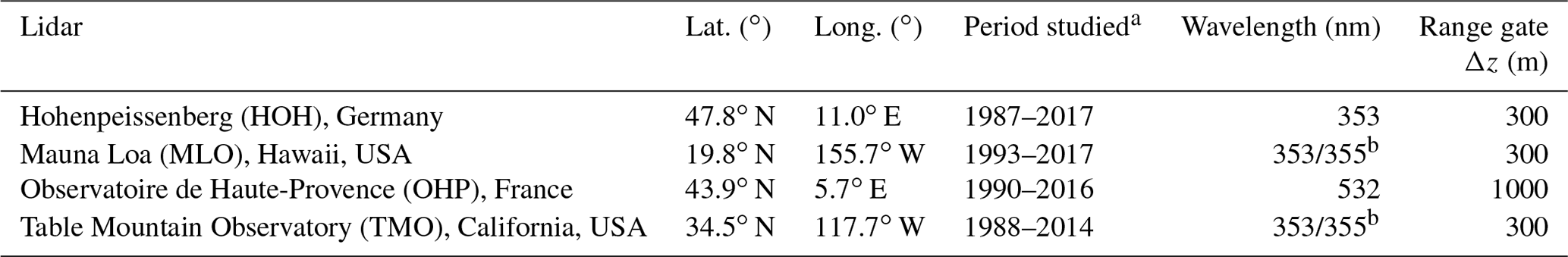
a based on data availability, b post 2001 upgrade
Validating Rayleigh temperature lidar measurements in the upper stratosphere and mesosphere can be difficult due to lack of reference temperature observations at these altitudes. Occasional comparisons with rocketsonde measurements showed temperature differences of 2–5 K in the lower mesosphere (Schmidlin, 1981; Ferrare et al., 1995). Over the past 2 decades, the performance of Rayleigh temperature lidars has been evaluated mainly by comparison with satellite measurements during which they served as the ground-based reference. These intercomparisons typically yield lidar-satellite differences not exceeding 2–4 K between 30 and 60 km (Wang et al., 1992; Ferrare et al., 1995; Wu et al., 2003; Sica et al., 2008; García-Comas et al., 2014; Stiller et al., 2012). At the bottom end of the profiles (below 30–35 km), the lidars have been compared to radiosonde measurements (Ferrare et al., 1995). In the presence of aerosols, Rayleigh backscatter lidars yield a significant cold bias (the thicker the aerosols, the colder the bias). The TMO and MLO instruments include an additional vibrational Raman backscatter channel, i.e. unimpacted by aerosol backscatter, which allows for temperature retrieval down to 10 km (Gross et al., 1997; Leblanc et al., 2016) but with a remaining slightly cold bias (1–4 K) due to aerosol extinction. For these two lidars, the reanalysis packages described in Sect. 2.3 will be compared for greater altitude ranges than the HOH and OHP lidars.
To fill the need for additional validation, one method frequently used within NDACC is to deploy a mobile lidar from site to site to blind test the lidar instruments permanently deployed at these locations. One such “travelling standard” is operated by the NASA Goddard Space Flight Centre (GSFC) (McGee et al., 1995) and has been used to validate the lidar instruments at HOH, OHP, TMO and MLO (Ferrare et al., 1995; Leblanc et al., 1998; Keckhut et al., 2004; Wing et al., 2020a, b). During these campaigns, temperature differences between the lidars did not exceed 4 K in the 25–60 km altitude range, with typical differences of ±2 K.
2.2 Microwave Limb Sounder
The NASA EOS MLS was launched on 14 July 2004 and became operational on 14 August 2004. It works by observing millimetre and sub-millimetre thermal emission along the limb of the atmosphere. It is in a low polar orbit, allowing it to orbit the Earth 15 times a day, crossing the Equator near to local noon and midnight. It is designed to measure several atmospheric gases and aerosols in the upper troposphere, stratosphere and mesosphere (Waters et al., 2006). It uses the emission from oxygen to provide temperature and pressure measurements; the precision of the measurement is given in Waters et al. (2006) to be 0.5–1 K between 300 and 0.001 hPa, where it has a vertical resolution between 4–8 km. Initial comparisons by Froidevaux et al. (2006) with other satellite retrievals of temperature found that EOS MLS had a 1–2 K warm bias. A more thorough comparison made by Schwartz et al. (2008) compared EOS MLS temperature retrievals to those from radiosondes and several satellites, including GPSRO. It was found that from 0.0001 to 0.3 hPa the temperature bias could range from −9 to 0 K with temperature precision ranging from ±1 to ±2.5 K. A further study by Wing et al. (2018) found that the bias in wintertime MLS was −10 K, and it was ±4 K in the summertime. At 1 hPa warm biases from 0 to 5 K were found. From 3.16 hPa down to 316 hPa, precision was found to be less than ±1 K, and biases were between −2 and 1.5 K. Thus, at pressure heights of 3 hPa and below, the EOS MLS satellite has a similar bias to that of the temperature lidar at the same observing height. Wing et al. (2020b) compared EOS MLS at the OHP lidar against NASA's reference lidar and it was found to have a large cold bias above 3 hPa of −10 K. Figure 1a–d show the mean MLS and lidar temperature profiles between 2004 and 2017 for HOH, MLO, OHP and TMO respectively. Panels e–h shows the average difference between the matched profiles at HOH, MLO, OHP and TMO respectively. This shows a cold bias which increases in magnitude with height and agrees well with the findings of Schwartz et al. (2008), Wing et al. (2018) and Wing et al. (2020b).
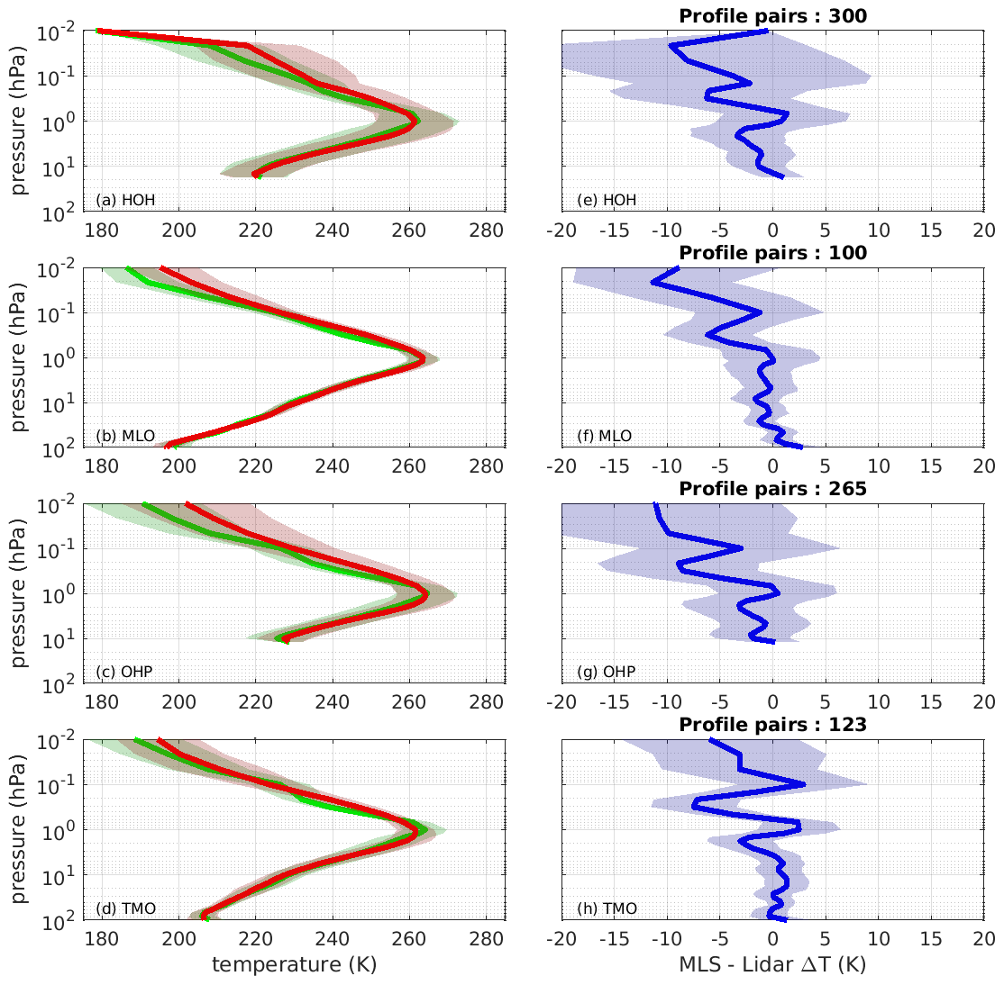
Figure 1Mean profiles of both temperature from EOS MLS (green) and Rayleigh temperature lidar (red) positioned at (a) Hohenpeissenberg, (b) Mauna Loa, (c) Observatoire de Haute-Provence and (d) Table Mountain Observatory. Shading depicts 1 standard deviation in the mean temperature. The vertical profiles of the mean of the differences between the lidar and MLS for the lidar shown in (a–b) are shown in (c–d) respectively; shading shows 1 standard deviation within the mean difference.
2.3 European Centre for Medium-Range Weather Forecasts data
A reanalysis dataset is generated by combining many different historical measurements using data assimilation to create an accurate numerical representation of the Earth's atmosphere at a given time. ERA-Interim spans from 1979 to 2019. ERA-Interim has 60 model levels spanning the surface to 0.3 hPa (57 km altitude) with an approximate 79 km horizontal grid resolution and 6 h analysis windows (Dee et al., 2011). It is based on the Integrated Forecasting System (IFS) cycle 31R2 and utilizes a 4Dvar data assimilation system. Dee et al. (2011) stated that during December 2006, GPSRO data from the COSMIC constellation were included in reanalysis datasets. Poli et al. (2010) showed that the variability in ERA-Interim temperature was much improved after this time.
ERA5 is the fifth-generation reanalysis created by the ECMWF and replaces ERA-Interim. The new ERA5 reanalysis, based on IFS cycle 41R2 (Hersbach et al., 2020), has 137 model levels from surface to 0.01 hPa (approximately 80 km) and a global horizontal resolution of 31 km, compared to ERA-Interim's 60 model levels and 79 km horizontal resolution. The ECMWF is constantly developing its IFS system, and 10 years of development since ERA-Interim has led to the inclusion of more measurement systems, improved bias correction techniques and model physics, CMIP5 radiative forcings, and data assimilation using a hybrid 4Dvar system (Hersbach et al., 2020). Simmons et al. (2020) showed that temperature bias in the upper stratosphere of ERA5 was significantly affected by the addition of AMSU-A data between 2000 and 2007 at heights above 15 hPa.
In this section MLS and lidar profiles are compared with temperature profiles from ERA-Interim. The lidar temperature profiles were interpolated onto ERA-Interim's model levels using geopotential height Z, for time steps that were closest to the midpoint of the lidar's profile acquisition period. To ensure the comparison was accurate, the lidar's geometric height coordinates were first converted to geopotential height. Despite being similar near ground level, the differences were between 0.4 and 1 km for the altitude ranges used in this study. The vertical resolution of ERA-Interim at these heights was approximately 1.5 km at 10 hPa and 3 km at 1 hPa. The comparison was undertaken using lidar and reanalysis profiles at each site for the operational periods given in column 4 of Table 1. Figure 2a–d show matched mean temperature profiles from both lidar (red) and ERA-Interim (blue) for the lidar sites at HOH, MLO, OHP and TMO respectively. Panels e–h show the mean of the matched differences for the corresponding profiles (a–d); grey shading shows 1 standard deviation in the matched differences. Crosses are red where the mean difference is different from zero at the 95 % significance level. For HOH, OHP and TMO, the peak cold bias is centred between 10 and 1 hPa. For MLO, the cold bias extends down to the 100 hPa pressure surface, whereas at TMO the cold bias is much closer to zero between 10 and 100 hPa. A possible hypothesis is that TMO is at a higher latitude than the tropically positioned MLO where the representation of the middle atmosphere within ERA-Interim differs slightly. For all sites, ERA-Interim exhibits a warm bias between 1 and 0.1 hPa. This contrastingly warm bias is due to the model top being reached and the stratopause not being represented. Panels i–l show the seasonal variation of the temperature biases with height. Both the warm bias near the model top and the cold bias between 1 and 10 hPa are present throughout the year, with the cold bias being strongest at all sites between November and February.
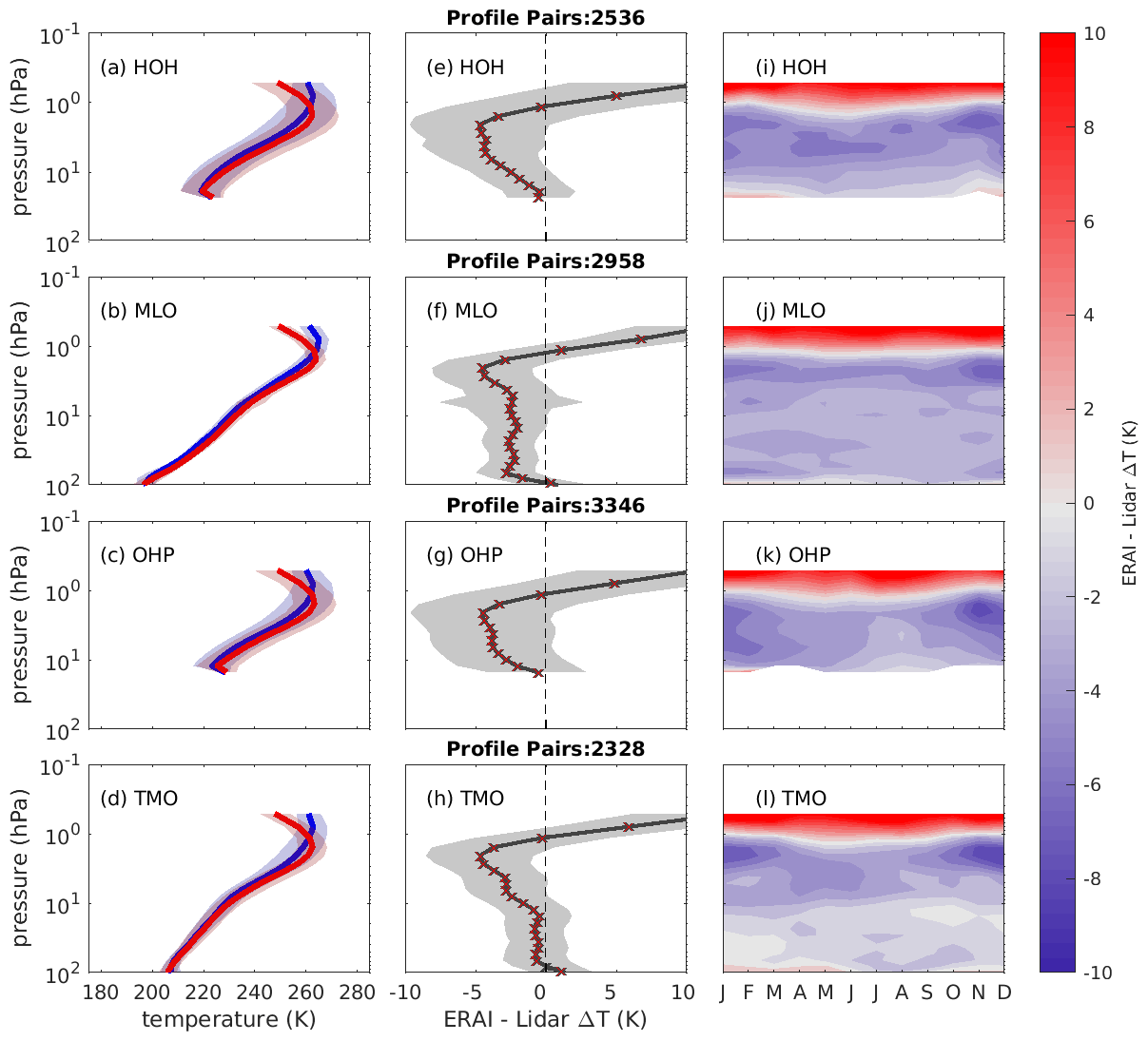
Figure 2Mean profiles of matched temperatures from ERA-Interim (blue) and Rayleigh temperature lidar (red) positioned at (a) Hohenpeissenberg, (b) Mauna Loa, (c) Observatoire de Haute-Provence and (d) Table Mountain Observatory between 1990 and 2017. Shading depicts 1 standard deviation in the mean temperature. The vertical profiles of the mean of the differences between ERA-Interim and each lidar shown in (a–d) are shown in (e–h) respectively; shading shows 1 standard deviation of mean difference. Crosses are red where the mean of the differences were different from zero at the 95 % significance level. Panels (i–l) show the temperature differences as a function of month and pressure level for each of the lidars shown in panels (a–d).
A similar analysis was performed using the EOS MLS data. The EOS MLS temperature data were first sorted so that only night-time passes within 2.5∘ of each temperature lidar site were retained. The remaining EOS MLS temperature profiles were interpolated onto ERA-Interim's model levels using Z for time steps that were closest and less than 3 h apart. Due to EOS MLS only being launched in 2004, the results of the ERA-Interim and MLS comparison shown in Fig. 3 are for the years 2004 to 2017. Figure 3 shows matched mean temperature profiles from both MLS (red) and ERA-Interim (blue) for lidar sites at HOH, MLO, OHP and TMO respectively. Panels e–h show the mean of the matched differences for MLS over the four lidar sites. The cold bias seen in Fig. 2 is not present when comparing with EOS MLS; instead a warm bias is present of approximately 1 K from 100 to 1 hPa at HOH, MLO and OHP. At TMO a cold bias of −1 to −2 K is observed at 1 hPa; the large warm bias above 1 hPa near the ERA-Interim model top shown in Fig. 2 is also observed. MLS shows a different temperature bias to that of the temperature lidar. Figure 1 showed that MLS has a cold bias when compared to the lidar at HOH and OHP and also in Schwartz et al. (2008), Wing et al. (2018) and Wing et al. (2020b). As the MLS records a negative bias when compared with the lidar, and ERA-Interim also exhibits a cold bias compared to the lidar, a resulting warm bias in the ERA-Interim comparison with MLS is observed. The cold bias seen at 1 hPa at TMO is due to the warm bias in MLS. The results seen here further demonstrates evidence of a systematic bias between the lidar and MLS measurement technologies at these heights. There is some oscillatory structure in the temperature bias that has been shown in Wing et al. (2018), who compared EOS MLS to lidar and found that the oscillations are not retrieval level dependent. Furthermore, the amplitude of the oscillations falls within the precision of EOS MLS given in Sect. 2.2
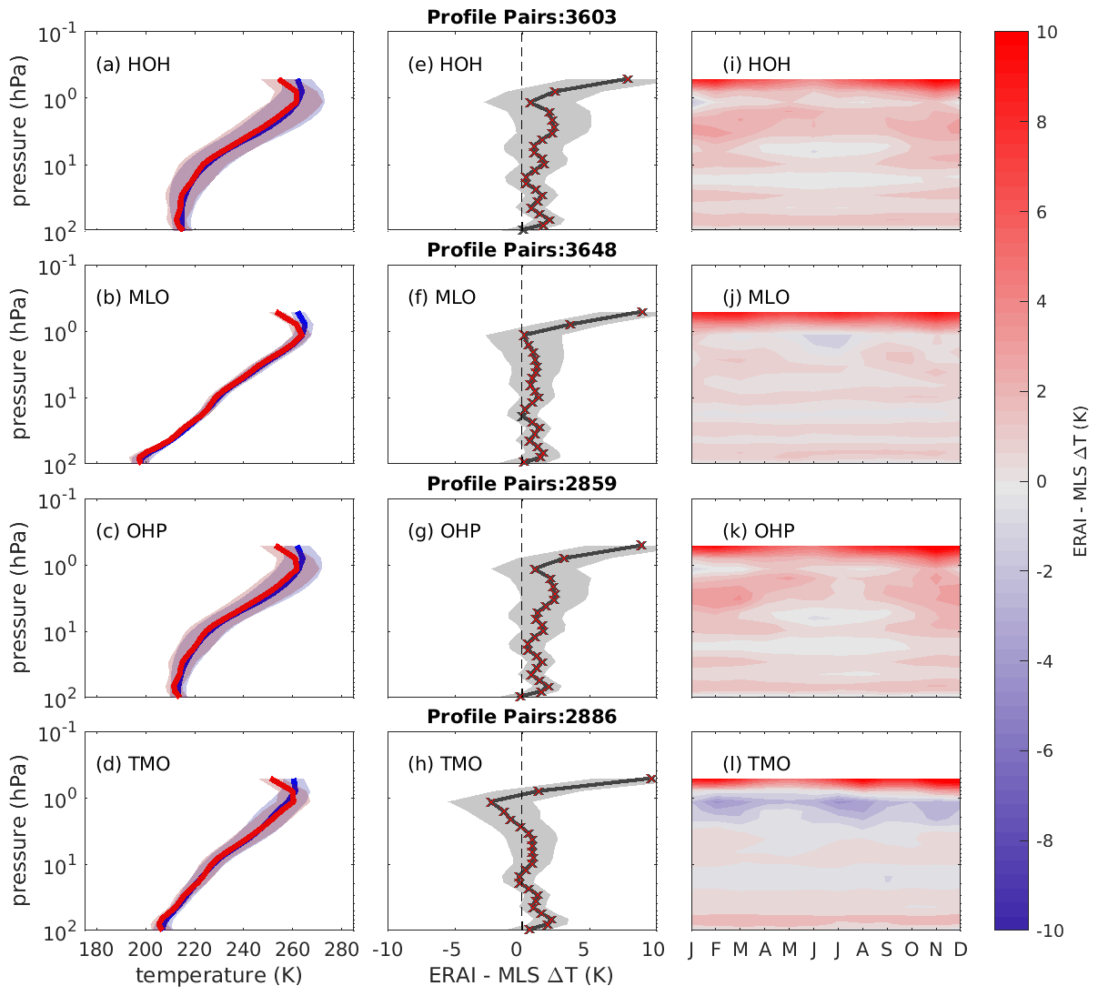
Figure 3Mean profiles of matched temperatures from ERA-Interim (blue) and EOS MLS passes (red) at (a) Hohenpeissenberg, (b) Mauna Loa, (c) Observatoire de Haute-Provence and (d) Table Mountain Observatory between 1990 and 2017. Shading depicts 1 standard deviation in the mean temperature. The vertical profiles of the mean of the differences between ERA-Interim and EOS MLS shown in (a–d) are shown in (e–h) respectively; shading shows 1 standard deviation of mean difference. Crosses are red for model levels where the mean of the differences are different from zero at the 95 % significance level. Panels (i–l) show the temperature differences as a function of month and pressure level for each of the lidars shown in panels (a–d).
Simmons et al. (2020) compared the global mean temperature from ERA-Interim with global mean radiosonde data between 15 and 7 hPa and at 7 hPa and above. The results in Fig. 2 agree with a cold bias seen in Simmons et al. (2020) for the height range 15–7 hPa, although the magnitude is much smaller. For 7 hPa and above, Simmons et al. (2020) found there was a warm bias of 1–2 K, whereas the results here for 7 to 1 hPa using the lidar have shown a cold bias at HOH, MLO and TMO. The temperature bias shown in Simmons et al. (2020) is a global mean, whereas the lidar measurements are made at fixed locations. Moreover, the bias was calculated using radiosonde data which are not independent as they are assimilated into ERA-Interim. This could explain the difference in sign in the results shown in this study.
In brief conclusion, the temperature lidars have shown that a cold bias of −3 to −4 K exists between 1 and 10 hPa in ERA-Interim for the HOH and OHP lidar sites and between 1 and 100 hPa for the TMO and MLO sites.
To compare the temperature biases in ERA5 with those in ERA-Interim, the comparison is repeated for ERA5 in a similar manner. The temperature lidar data were interpolated, accounting for geometric height, onto ERA5 model levels using Z for the nearest analysis window to the midpoint of the lidar acquisition window. The vertical resolution or ERA5 at 10 hPa was 750 m and at 1 hPa was 1.6 km. Figure 4a–d show the mean temperature profiles for the lidar in red and ERA5 in blue up to a height of 0.5 hPa for the period 1990–2017. At first inspection ERA5 profiles track the lidar profiles more closely than those of ERA-Interim, including a more accurate representation of the stratopause than that of ERA-Interim (see Fig. 2). Figure 4e–h show the mean of matched differences with height; grey shading shows 1 standard deviation in the matched differences, and crosses are red where the mean difference is different from zero at the 95 % significance level inferred by a single sample t test. The temperature biases are significantly smaller than in ERA-Interim. For the MLO and TMO sites, the temperature bias is very close to zero up to the 10 hPa pressure surface. At 10 to 5 hPa, a cold bias of −1 to −2 K is observed at all sites. From 5 to 1 hPa, the bias drops to near zero again and above 1 hPa a −3 K cold bias is observed at all four sites. When considering that the measurement accuracy of the lidar is ±2 K, ERA5 gives a good thermal representation of the atmosphere up to 1 hPa. Figure 4i–l shows the seasonal variation of temperature bias with height. For all four sites, there is a slight warm bias of approximately 1 K at 1–5 hPa during the summer months (May–August) with the exception of MLO where the warm bias at this height spans January to July. The cold bias above 1 hPa intensifies in the winter months.
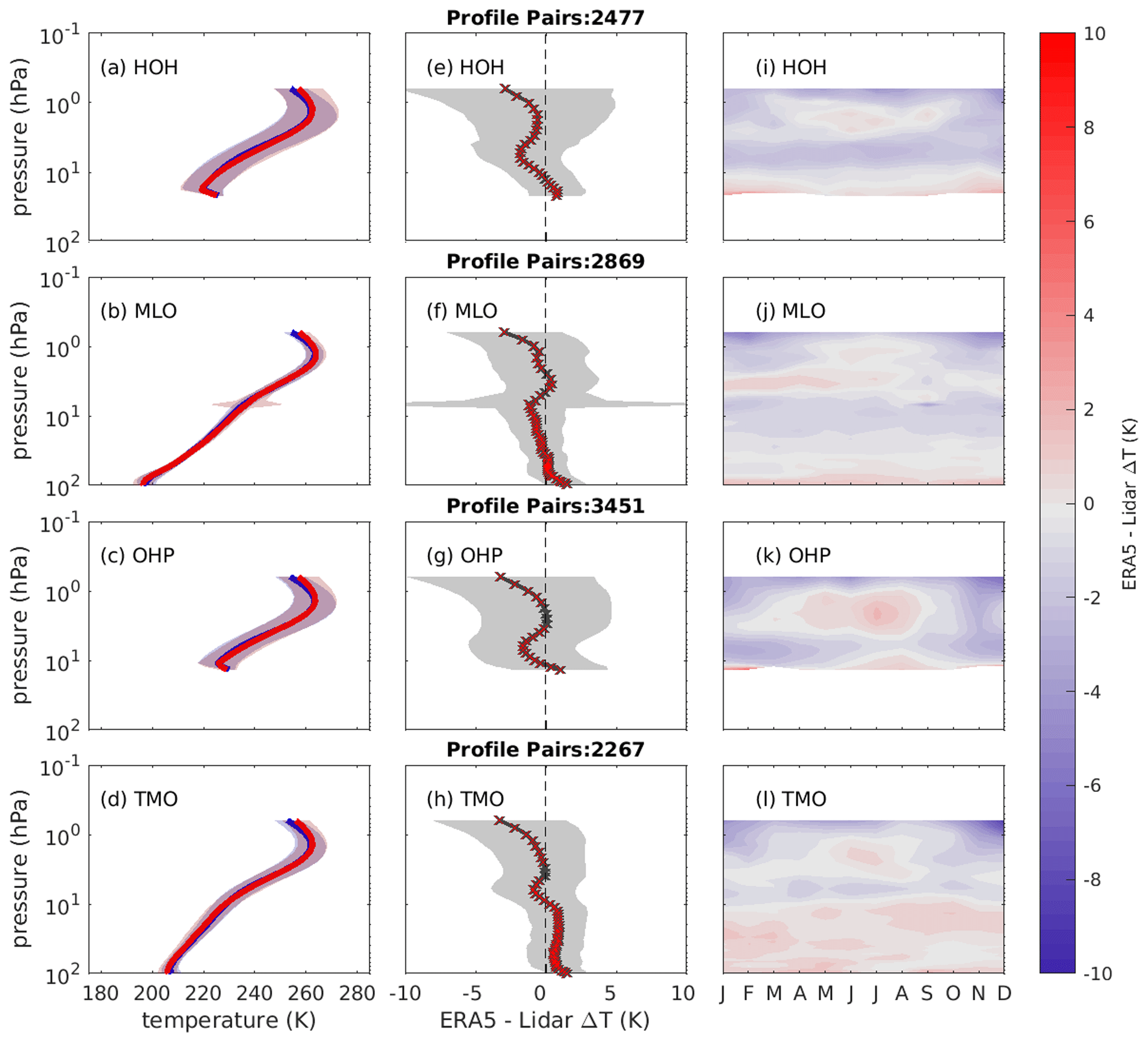
Figure 4Mean profiles of matched temperatures from ERA5 (blue) and Rayleigh temperature lidar (red) positioned at (a) Hohenpeissenberg, (b) Mauna Loa, (c) Observatoire de Haute-Provence and (d) Table Mountain Observatory between 1990 and 2017. Shading depicts 1 standard deviation in the mean temperature. The vertical profiles of the mean of the differences between ERA5 and each lidar shown in (a–d) are shown in (e–h) respectively; shading shows 1 standard deviation of mean difference. Crosses are red for model levels where the mean of the differences are different from zero at the 95 % significance level. Panels (i–l) show the temperature differences as a function of month and pressure level for each of the lidars shown in panels (a–d).
Figure 5 shows the temperature comparisons against MLS for the period 2004 to 2017; the data was interpolated onto the ERA5 model levels using the same method as discussed in Sect. 3. MLS and ERA5 show a fair agreement at all sites between 100 and 10 hPa, but not as good as with that of the lidar at TMO and MLO. From 100 to 5 hPa, there is a warm bias which varies with amplitude between 1–2 K. The warm bias peaks at 3 hPa with an amplitude of 3 K, while at 1 hPa and above a large cold bias of −5 K is found. Panels i–l show that there is little seasonal variation in the temperature bias between ERA5 and MLS. Given the findings of Schwartz et al. (2008), Wing et al. (2018) and Fig. 1, it is clear that these bias are largely due to the MLS temperature bias previously discussed in Sect. 2.2.
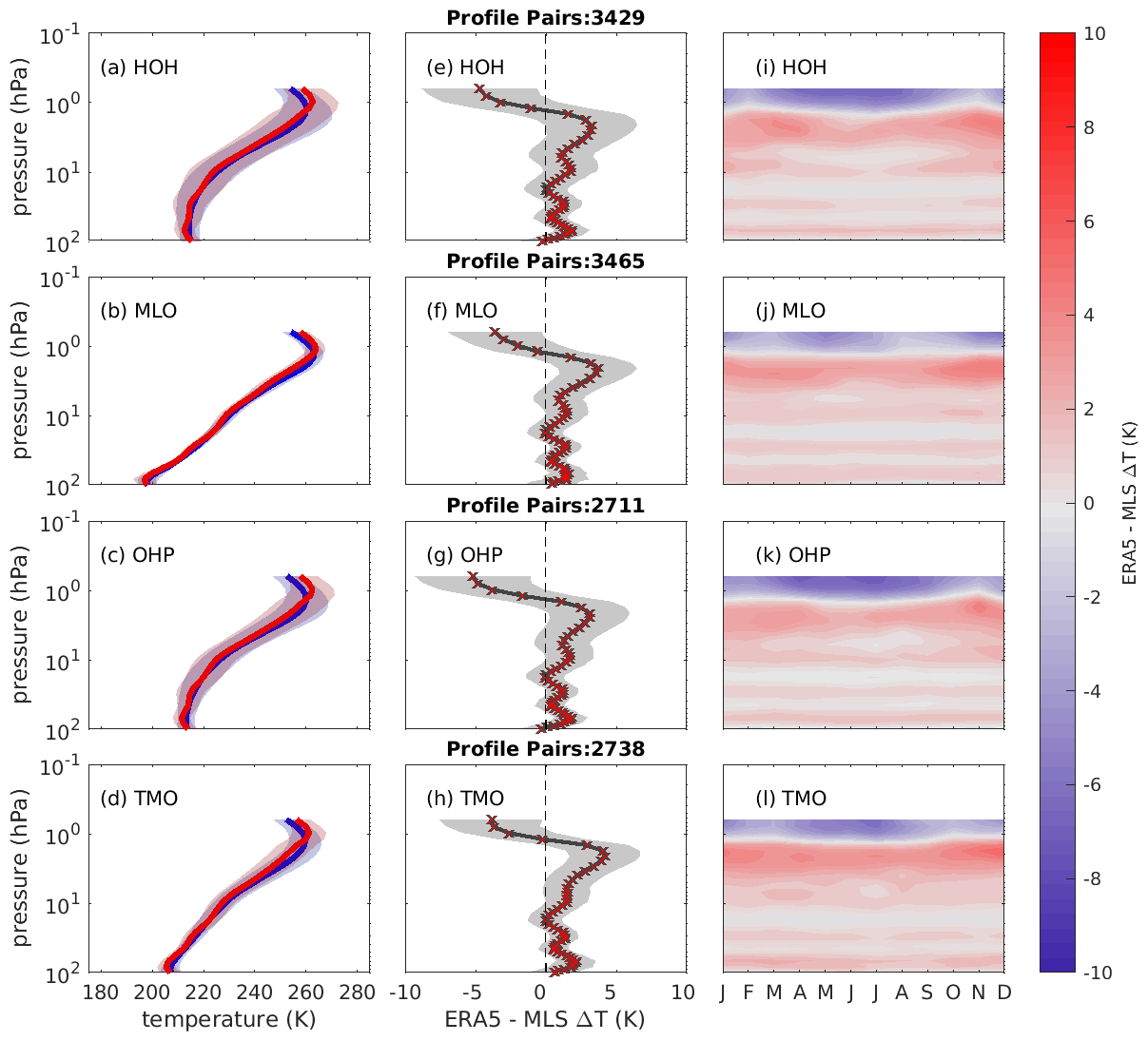
Figure 5Mean profiles of matched temperatures from ERA5 (blue) and EOS MLS passes (red)at (a) Hohenpeissenberg, (b) Mauna Loa, (c) Observatoire de Haute-Provence and (d) Table Mountain Observatory between 1990 and 2017. Shading depicts 1 standard deviation in the mean temperature. The vertical profiles of the mean of the differences between ERA5 and EOS MLS are shown in (a–d) are shown in (e–h) respectively; shading shows 1 standard deviation of mean difference. Crosses are red for model levels where the mean of the differences are different from zero at the 95 % significance level. Panels (i–l) show the temperature differences as a function of month and pressure level for each of the lidars shown in panels (a–d).
Simmons et al. (2020) compared the global mean temperature from ERA5 with global mean radiosonde data from 15 hPa upwards and found that performance was similar to ERA-Interim pre 2000. A warm bias of 2 K was found above 7 hPa and a slight cold bias of less than −0.5 K between 7 and 15 hPa for ERA5. Between 2000 and 2007 there was an increase in the warm bias making the bias 3 and 0.5 K for the layers 7 hPa and above and 7–15 hPa respectively. Simmons et al. (2020) believed that this may be due to the introduction of observations from the AMSU-A instrument aboard NOAA-15 and NOAA-16 (Aumann et al., 2003) from 2000. Post 2007, after the introduction of GPSRO data, Simmons et al. (2020) showed the temperature bias above 7 hPa to be 1.5 K and less than 0.5 K between 7–15 hPa. As the time period of this study spans 1990 to 2017, some aspects of the analysis by Simmons et al. (2020) are shown in that a warm bias is observed above 7 hPa during the summer months. It has been shown that ERA5 gives a much improved thermal representation of the upper stratosphere when compared to ERA-Interim. The focus has been on calculating temperature bias over a 1990–2017 and 2004–2017 study period for the lidar and MLS respectively. This means it is difficult to see if a particular data stream improved ERA-Interim or ERA5's representation of the upper stratosphere. Given that the lidars have made measurements for over 25 years, the dataset can be further examined by year to see how the introduction of new observation streams such as GPSRO and AMSU-A affected the ERA datasets.
The mean of differences between lidar and both ERA-Interim and ERA5 were decomposed by year to examine if the introduction of new satellite data streams such as COSMIC GPSRO and AMSU-A changed the stratospheric temperature bias. Poli et al. (2010) showed that the inclusion of COSMIC GPSRO data improved reanalysis bias in the upper troposphere and lower stratosphere. However, their comparison was only undertaken between 200 and 100 hPa. The effect of the inclusion of COSMIC GPSRO at 100 hPa was described in Cardinali and Healy (2014), who found a decrease in forecast error between 250 and 50 hPa. Simmons et al. (2020) showed a change in ERA5 temperature bias after the inclusion of the AMSU-A satellite data in 1999/2000. Data from MLS are only available post 2004, and since AMSU-A data became available in 1998 we restrict our time series analysis to comparisons with the lidar only.
Figure 6 shows the average annual temperature difference as a function of year and height between ERA-Interim and the temperature lidar. HOH, OHP and TMO show an elevated cold bias between 1 and 10 hPa until 1995–1996. It is not known if this occurred at MLO, due to lack of data over this period. Figure 14 in Dee et al. (2011) shows that during this 1995/1996 period, the NOAA-14 SSU unit was launched and added to the data assimilation streams. This could explain the decrease in the cold bias at the 1 to 10 hPa pressure range. During the 1998/1999 period, a warm bias, similar to that experienced at the model top, formed around the 1 hPa pressure level, which coincided with the inclusion of AMSU-A satellite data in 1998. Simmons et al. (2020) discussed how the addition of AMSU-A affected ERA-Interim. It is apparent here it may have increased the warm bias of ERA-Interim at 1 hPa. HOH and TMO show subtle reductions in the cold bias from −5 to −4 in the 10–1 hPa range post 2007. With the exception of OHP, which has an intensified cold bias between 2014 and 2017, there are no further significant changes in temperature bias over the studied period.
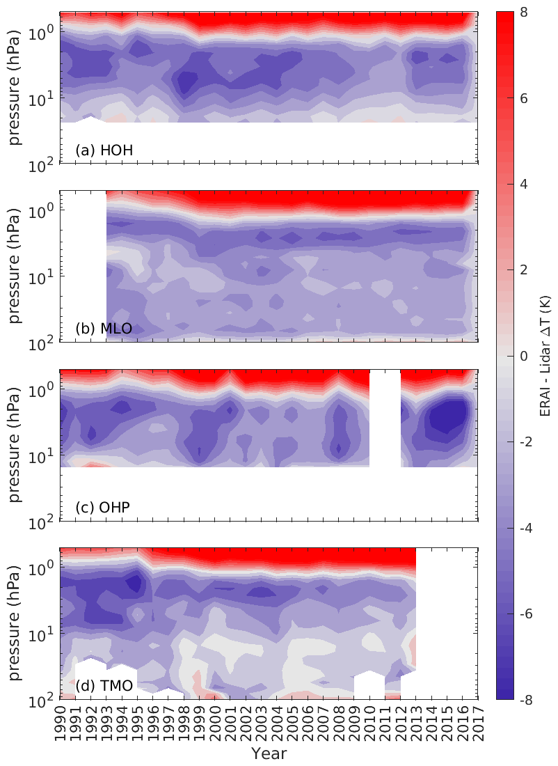
Figure 6Annual Temperature bias between ERA-Interim and temperature lidars at (a) Hohenpeissenberg, (b) Mauna Loa, (c) Observatoire de Haute-Provence and (d) Table Mountain Observatory plotted as a function of year and height between 1990 and 2017. Data gaps are given by white blocks.
Figure 7 shows the average annual temperature difference as a function of year and height between ERA5 and the temperature lidar. In the 3–5 hPa range at all sites there was a warm bias of 2–3 K between 1994 and 1997/1998. The abrupt and consistent reduction of the warm bias at all sites during 1998 corresponded with the advent of NOAA-15 AMSU-A data, suggesting that assimilation of this data stream caused the reduced bias. However, by 2000 the warm bias returned at this height range and was most dominant at OHP and TMO. One explanation could be that the addition of AMSU-A aboard NOAA-16 which was assimilated between the years of 2001–2009 (Hersbach et al., 2020) caused this warm bias, agreeing with the conclusions in Simmons et al. (2020). The cold bias at 1 hPa at HOH, MLO and TMO reduced from −2 to near 0 K at the end of 2006, which coincided with COSMIC GPSRO being made available for assimilation from December 2006. Although GPSRO has a tangent height of 50 km, the assimilation of the bending angle means it can contribute observations at higher altitudes than 50 km (Healy, 2008). Additionally the hydrostatic nature of the model means that observations assimilated at a given level affect those above and below.
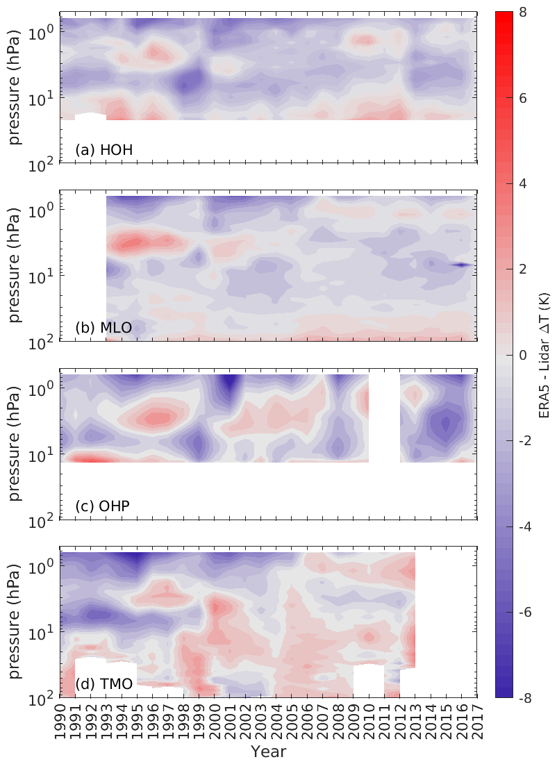
Figure 7Annual temperature bias between ERA5 and temperature lidars at (a) Hohenpeissenberg, (b) Mauna Loa, (c) Observatoire de Haute-Provence and (d) Table Mountain Observatory plotted as a function of year and height between 1990 and 2017. Data gaps are given by white blocks.
In summary, the cold temperature bias in ERA5 above 1 hPa was reduced from −2 to near 0 K at 3 out of 4 of the sites post 2007 due to the inclusion of GPSRO data. Inclusion of the AMSU-A data on NOAA-15 from 1998 appears to have reduced the warm bias at 3 hPa. This warm bias reappears at some sites with the introduction of AMSU-A data from NOAA-16. Although the instruments on both satellites are similar, inter-satellite brightness temperature bias has been shown before by Mo (2011) between the AMSU-A units on both NOAA-18 and NOAA-19 satellites. This could explain the opposing bias seen here. OHP and TMO show an intensification of the warm bias between 2000 and 2007 between 10–1 hPa, showing agreement with findings of Simmons et al. (2020).
In this work temperature lidar data from NDACC, which are not assimilated into reanalyses, have been utilized to identify temperature bias in the upper stratosphere in ERA-Interim and ERA5 reanalyses. Comparisons with ERA-Interim and the lidar have shown a cold bias of −3 to −4 K between 10 and 1 hPa and a large warm bias above 1 hPa. The cold bias intensified in Northern Hemisphere winter to −5 to −6 K. For ERA5, the temperature bias between the lidar and ERA5 was within ±1 K to a height of 1 hPa, which given the measurement accuracies of the lidar ± 2 K gives a good thermal representation of the stratosphere. Above 1 hPa a cold bias of −2 to −3 K was found. Similar to ERA-Interim, the ERA5 cold bias above 1 hPa intensifies to −4 K in the Northern Hemisphere winter months and became a warm bias in the summer months. When comparing to MLS, ERA-Interim exhibited a warm bias of 1 K and ERA5 had a warm bias of 1–2 K up to 5 hPa. Above this height, MLS's warm bias at 3 hPa and the large cold bias at 1 hPa, both shown here in Fig. 1, (Schwartz et al., 2008; Wing et al., 2018) become predominant in the temperature bias results.
When examining the ERA-Interim lidar comparison over 1990–2017, a warm bias increase occurred at 1 hPa around 1997/1998, which could be due to the introduction of AMSU-A. There was also a small reduction from −5 to −4 K post 2006 which is most noticeable at 1–2 hPa at HOH and TMO. This could be an indication that the inclusion of COSMIC GPSRO has an effect on the upper stratosphere within ERA-Interim. For ERA5, the effects of new satellites being assimilated was clearer. We see that the inclusion of the two AMSU-A data streams had an effect on temperature bias between 1–10 hPa. It appears that during 1998 the assimilation of AMSU-A from NOAA-15 reduced the warm bias. Yet, when AMSU-A from NOAA-16 was assimilated in 2000–2009 the warm bias returned. However, it was not as intense. Post 2007, a reduction in the cold bias above 1 hPa was observed at HOH, MLO and TMO due to the assimilation of COSMIC GPSRO. Other small changes in the temperature bias seen in Figs. 6 and 7 could be attributed to other observations being assimilated. Both Hersbach et al. (2020) and Dee et al. (2011) show that in both ERA5 and ERA-Interim the number and type of observations increase with time, making it harder to attribute behaviours in the upper stratospheric temperature bias to a particular observation dataset.
From the comparisons here, it can be stated that ERA5 is much improved compared to ERA-Interim and has a good thermodynamic representation of the upper stratosphere. When considering the uncertainties in the lidar, ERA5 is an excellent choice for further stratospheric studies or for the use as reference to compare to other reanalyses. However, a cold bias detected in ERA5 by the lidar before the inclusion of GPSRO and AMSU-A data should be accounted for in studies such as Shangguan et al. (2019) and Bohlinger et al. (2014). These studies used both ERA5 and ERA-Interim to assess long-term and short-term stratospheric temperature variability. In future works exploring stratospheric temperature trends, changes in temperature biases presented here need to be considered.
The temperature lidars, whilst limited to a few locations globally, have made high vertical resolution temperature measurements for nearly 30 years, making them an important and useful tool for inferring temperature biases in reanalysis datasets, which span similar time periods. A future test could see the lidar networks used to explore modifications to reanalysis datasets such as testing the experimental ERA5.1 discussed in Simmons et al. (2020).
The data used in this publication were obtained from Thierry Leblanc, Wolfgang Steinbrecht and Robin Wing as part of the Network for the Detection of Atmospheric Composition Change (NDACC) and are available through the NDACC website http://www.ndacc.org/ (last access: April 2018). The Microwave Limb Sounder data are available for public download at https://doi.org/10.5067/Aura/MLS/DATA2520 (Schwartz et al., 2020). ECMWF ERA-Interim and ERA5 data are available from the ECMWF MARS archive.
GM extracted the datasets, performed the analysis and prepared the article. RW provided and processed the OHP data. ACP, GH, IP, AH and PK provided inputs for the analysis and preparation of the article. TL provided MLO and TMO data and assisted with article preparation. WS provided the HOH data and assisted with article preparation.
The authors declare that they have no conflict of interest.
This article is part of the special issue “The SPARC Reanalysis Intercomparison Project (S-RIP) (ACP/ESSD inter-journal SI)”. It is not associated with a conference.
This work was performed during the course of the ARISE2 collaborative infrastructure design study project (http://arise-project.eu/, last access: 13 April 2021). The authors also wish to acknowledge staff at the ECMWF for their discussions as this work advanced.
This research has been supported by the European Commission H2020 programme (grant no. 653980).
This paper was edited by Geraint Vaughan and reviewed by two anonymous referees.
Aumann, H. H., Chahine, M. T., Gautier, C., Goldberg, M. D., Kalnay, E., McMillin, L. M., Revercomb, H., Rosenkranz, P. W., Smith, W. L., Staelin, D. H., Strow, L. L., and Susskind, J.: AIRS/AMSU/HSB on the Aqua mission: Design, science objectives, data products, and processing systems, IEEE T. Geosci. Remote, 41, 253–264, 2003. a
Baldwin, M. P., Gray, L. J., Dunkerton, T. J., Hamilton, K., Haynes, P. H., Randel, W. J., Holton, J. R., Alexander, M. J., Hirota, I., Horinouchi, T., Jones, D. B. A., Kinnersley, J. S., Marquardt, C., Sato, K., and Takahashi, M.: The quasi-biennial oscillation, Rev. Geophys., 39, 179–229, 2001. a
Bohlinger, P., Sinnhuber, B.-M., Ruhnke, R., and Kirner, O.: Radiative and dynamical contributions to past and future Arctic stratospheric temperature trends, Atmos. Chem. Phys., 14, 1679–1688, https://doi.org/10.5194/acp-14-1679-2014, 2014. a
Butler, A. H., Seidel, D. J., Hardiman, S. C., Butchart, N., Birner, T., and Match, A.: Defining sudden stratospheric warmings, B. Am. Meteorol. Soc., 96, 1913–1928, 2015. a
Cardinali, C. and Healy, S.: Impact of GPS radio occultation measurements in the ECMWF system using adjoint-based diagnostics, Q. J. Roy. Meteorol. Soc., 140, 2315–2320, 2014. a
Chandra, S., Fleming, E. L., Schoeberl, M. R., and Barnett, J. J.: Monthly mean global climatology of temperature, wind, geopotential height and pressure for 0–120 km, Adv. Space Res., 10, 3–12, https://doi.org/10.1016/0273-1177(90)90230-W, 1990. a
Charlton, A. J. and Polvani, L. M.: A new look at stratospheric sudden warmings. Part I: Climatology and modeling benchmarks, J. Climate, 20, 449–469, 2007. a
Dee, D., Uppala, S., Simmons, A., Berrisford, P., Poli, P., Kobayashi, S., Andrae, U., Balmaseda, M., Balsamo, G., Bauer, P., Bechtold, P., Beljaars, A. C. M., van de Berg, L., Bidlot, J., Bormann, N., Delsol, C., Dragani, R., Fuentes, M., Geer, A. J., Haimberger, L., Healy, S. B., Hersbach, H., Hólm, E. V., Isaksen, L., Kållberg, P., Köhler, M., Matricardi, M., McNally, A. P., Monge-Sanz, B. M., Morcrette, J.-J., Park, B.-K., Peubey, C., de Rosnay, P., Tavolato, C., Thépaut, J.-N., and Vitart, F.: The ERA-Interim reanalysis: Configuration and performance of the data assimilation system, Q. J. Roy. Meteorol. Soc., 137, 553–597, 2011. a, b, c, d, e
Domeisen, D. I.: Estimating the frequency of sudden stratospheric warming events from surface observations of the North Atlantic Oscillation, J. Geophys. Res.-Atmos., 124, 3180–3194, 2019. a
Domeisen, D. I., Garfinkel, C. I., and Butler, A. H.: The teleconnection of El Niño Southern Oscillation to the stratosphere, Rev. Geophys., 57, 5–47, 2019. a
Ferrare, R., McGee, T., Whiteman, D., Burris, J., Owens, M., Butler, J., Barnes, R., Schmidlin, F., Komhyr, W., Wang, P. H., McCormick, M. P., and Mille, A. J.: Lidar measurements of stratospheric temperature during STOIC, J. Geophys. Res.-Atmos., 100, 9303–9312, 1995. a, b, c, d, e
Froidevaux, L., Livesey, N. J., Read, W. G., Jiang, Y. B., Jimenez, C., Filipiak, M. J., Schwartz, M. J., Santee, M. L., Pumphrey, H. C., Jiang, J. H., Wu, D. L., Manney, G. L., Drouin, B. J., Waters, J. W., Fetzer, E. J., Bernath, P. F., Boone, C. D., Walker, K. A., Jucks, K. W., Toon, G. C., Margitan, J. J., Sen, B., Webster, C. R., Christensen, L. E., Elkins, J. W., Atlas, E., Lueb, R. A., and Hendershot, R.: Early validation analyses of atmospheric profiles from EOS MLS on the Aura satellite, IEEE T. Geosci. Remote, 44, 1106–1121, 2006. a
Fujiwara, M., Wright, J. S., Manney, G. L., Gray, L. J., Anstey, J., Birner, T., Davis, S., Gerber, E. P., Harvey, V. L., Hegglin, M. I., Homeyer, C. R., Knox, J. A., Krüger, K., Lambert, A., Long, C. S., Martineau, P., Molod, A., Monge-Sanz, B. M., Santee, M. L., Tegtmeier, S., Chabrillat, S., Tan, D. G. H., Jackson, D. R., Polavarapu, S., Compo, G. P., Dragani, R., Ebisuzaki, W., Harada, Y., Kobayashi, C., McCarty, W., Onogi, K., Pawson, S., Simmons, A., Wargan, K., Whitaker, J. S., and Zou, C.-Z.: Introduction to the SPARC Reanalysis Intercomparison Project (S-RIP) and overview of the reanalysis systems, Atmos. Chem. Phys., 17, 1417–1452, https://doi.org/10.5194/acp-17-1417-2017, 2017. a
García-Comas, M., Funke, B., Gardini, A., López-Puertas, M., Jurado-Navarro, A., von Clarmann, T., Stiller, G., Kiefer, M., Boone, C. D., Leblanc, T., Marshall, B. T., Schwartz, M. J., and Sheese, P. E.: MIPAS temperature from the stratosphere to the lower thermosphere: Comparison of vM21 with ACE-FTS, MLS, OSIRIS, SABER, SOFIE and lidar measurements, Atmos. Meas. Tech., 7, 3633–3651, https://doi.org/10.5194/amt-7-3633-2014, 2014. a
Gross, M. R., McGee, T. J., Ferrare, R. A., Singh, U. N., and Kimvilakani, P.: Temperature measurements made with a combined Rayleigh–Mie and Raman lidar, Appl. Opt., 36, 5987–5995, 1997. a
Hauchecorne, A.: Lidar Temperature Measurements in the Middle Atmosphere, Rev. Laser Eng., 23, 119–123, 1995. a
Hauchecorne, A. and Chanin, M.-L.: Density and temperature profiles obtained by lidar between 35 and 70 km, Geophys. Res. Lett., 7, 565–568, 1980. a, b
Healy, S.: Assimilation of GPS radio occultation measurements at ECMWF, in: Proceedings of the GRAS SAF Workshop on Applications of GPSRO measurements, ECMWF, Reading, UK, pp. 16–18, 2008. a
Hersbach, H., Bell, B., Berrisford, P., Hirahara, S., Horányi, A., Muñoz-Sabater, J., Nicolas, J., Peubey, C., Radu, R., Schepers, D., Simmons, A., Soci, C., Abdalla, S., Abellan, X., Balsamo, G., Bechtold, P., Biavati, G., Bidlot, J., Bonavita, M., De Chiara, G., Dahlgren, P., Dee, D., Diamantakis, M., Agani, R., Flemming, J., Forbes, R., Fuentes, M., Geer, A., Haimberger, L., Healy, S., Hogan, R. J., Hólm, E., Janisková, M., Keeley, S., Laloyaux, P., Lopez, C., Radnoti, G., de Rosnay, P., Rozum, I., Vamborg, F., Villaume, S., and Thépau, J.-N.: The ERA5 global reanalysis, Q. J. Roy. Meteorol. Soc., 146, 1999–2049, 2020. a, b, c, d
Jenkins, D., Wareing, D., Thomas, L., and Vaughan, G.: Upper stratospheric and mesospheric temperatures derived from lidar observations at Aberystwyth, J. Atmos. Terr. Phys., 49, 287–298, 1987. a
Kalnay, E., Kanamitsu, M., Kistler, R., Collins, W., Deaven, D., Gandin, L., Iredell, M., Saha, S., White, G., Woollen, J., Zhu, Y., Chelliah, M., Ebisuzaki, W., Higgins, W., Janowiak, J., Mo, K. C., Ropelewski, C., Wang, J., Leetmaa, A., Reynolds, R., Jenne, R., and Joseph, D.: The NCEP/NCAR 40-year reanalysis project, B. Am. Meteorol. Soc., 77, 437–471, 1996. a
Keckhut, P., McDermid, S., Swart, D., McGee, T., Godin-Beekmann, S., Adriani, A., Barnes, J., Baray, J.-L., Bencherif, H., Claude, H., di Sarra, A. G., Fiocco, G., Hansen, G., Hauchecorne, A., Leblanc, T., Lee, C. H., Pal, S., Megie, G., Nakane, H., Neuber, R., Steinbrecht, W., and Thayer, J.: Review of ozone and temperature lidar validations performed within the framework of the Network for the Detection of Stratospheric Change, J. Environ. Monit., 6, 721–733, 2004. a
Kuo, Y.-H., Sokolovskiy, S. V., Anthes, R. A., and Vandenberghe, F.: Assimilation of GPS radio occultation data for numerical weather prediction, Terr. Atmos. Ocean. Sci., 11, 157–186, 2000. a
Le Pichon, A., Assink, J., Heinrich, P., Blanc, E., Charlton-Perez, A., Lee, C. F., Keckhut, P., Hauchecorne, A., Rüfenacht, R., Kämpfer, N., Drob, D. P., Smets, P. S. M., Evers, L. G., Ceranna, L., Pilger, C., Ross, O., and Claud, C.: Comparison of co-located independent ground-based middle atmospheric wind and temperature measurements with numerical weather prediction models, J. Geophys. Res.-Atmos., 120, 8318–8331, 2015. a
Leblanc, T., McDermid, I. S., Hauchecorne, A., and Keckhut, P.: Evaluation of optimization of lidar temperature analysis algorithms using simulated data, J. Geophys. Res.-Atmos., 103, 6177–6187, 1998. a
Leblanc, T., Sica, R. J., van Gijsel, J. A. E., Haefele, A., Payen, G., and Liberti, G.: Proposed standardized definitions for vertical resolution and uncertainty in the NDACC lidar ozone and temperature algorithms – Part 3: Temperature uncertainty budget, Atmos. Meas. Tech., 9, 4079–4101, https://doi.org/10.5194/amt-9-4079-2016, 2016. a, b, c
Lee, C., Smets, P., Charlton-Perez, A., Evers, L., Harrison, G., and Marlton, G.: The potential impact of upper stratospheric measurements on sub-seasonal forecasts in the extra-tropics, in: Infrasound Monitoring for Atmospheric Studies, pp. 889–907, Springer, 2019. a
Li, T., Leblanc, T., and McDermid, I. S.: Interannual variations of middle atmospheric temperature as measured by the JPL lidar at Mauna Loa Observatory, Hawaii (19.5∘ N, 155.6∘ W), J. Geophys. Res.-Atmos., 113, D14109, https://doi.org/10.1029/2007JD009764, 2008. a
McGee, T. J., Ferrare, R. A., Whiteman, D. N., Butler, J. J., Burris, J. F., and Owens, M. A.: Lidar measurements of stratospheric ozone during the STOIC campaign, J. Geophys. Res.-Atmos., 100, 9255–9262, 1995. a
Miller, D., Brownscombe, J., Carruthers, G., Pick, D., and Stewart, K.: Operational temperature sounding of the stratosphere, Philos. T. Roy. Soc. Lond. A, 296, 65–71, 1980. a
Mo, T.: Calibration of the NOAA AMSU-A radiometers with natural test sites, IEEE T. Geosci. Remote, 49, 3334–3342, 2011. a
Picone, J. M., Hedin, A. E., Drob, D. P., and Aikin, A. C.: NRLMSISE-00 empirical model of the atmosphere: Statistical comparisons and scientific issues, J. Geophys. Res.-Space Phys., 107, 15–16, https://doi.org/10.1029/2002JA009430, 2002. a
Poli, P., Healy, S., and Dee, D.: Assimilation of Global Positioning System radio occultation data in the ECMWF ERA–Interim reanalysis, Q. J. Roy. Meteorol. Soc., 136, 1972–1990, 2010. a, b, c
Russell, J. M., Mlynczak, M. G., Gordley, L. L., Tansock, J. J., and Esplin, R. W.: Overview of the SABER experiment and preliminary calibration results, in: Optical Spectroscopic Techniques and Instrumentation for Atmospheric and Space Research III, vol. 3756, pp. 277–289, International Society for Optics and Photonics, 1999. a
Schmidlin, F. J.: Repeatability and measurement uncertainty of the United States meteorological rocketsonde, J. Geophys. Res.-Oceans, 86, 9599–9603, 1981. a, b
Schwartz, M. J., Lambert, A., Manney, G. L., Read, W. G., Livesey, N. J., Froidevaux, L., Ao, C. O., Bernath, P. F., Boone, C. D., Cofield, R. E., Daffer, W. H., Drouin, B. J., Fetzer, E. J., Fuller, R. A., Jarnot, R. F., Jiang, J. H., Jiang, Y. B., Knosp, B. W., Krüger, K., Li, J.‐L. F., Mlynczak, M. G., Pawson, S., Russell III, J. M., Santee, M. L., Snyder, W. V., Stek, P. C., Thurstans, R. P., Tompkins, A. M., Wagner, P. A., Walker, K. A., Waters, J., and Wu, D. L.: Validation of the Aura Microwave Limb Sounder temperature and geopotential height measurements, J. Geophys. Res.-Atmos., 113, D15S11, https://doi.org/10.1029/2007JD008783, 2008. a, b, c, d, e
Schwartz, M., Livesey, N., and Read, W.: MLS/Aura Level 2 Temperature V005, Greenbelt, MD, USA, Goddard Earth Sciences Data and Information Services Center (GES DISC), https://doi.org/10.5067/Aura/MLS/DATA2520, 2020. a
Seviour, W. J., Butchart, N., and Hardiman, S. C.: The Brewer–Dobson circulation inferred from ERA-Interim, Q. J. Roy. Meteorol. Soc., 138, 878–888, 2012. a
Shangguan, M., Wang, W., and Jin, S.: Variability of temperature and ozone in the upper troposphere and lower stratosphere from multi-satellite observations and reanalysis data, Atmos. Chem. Phys., 19, 6659–6679, https://doi.org/10.5194/acp-19-6659-2019, 2019. a
Sheng, Z., Jiang, Y., Wan, L., and Fan, Z.: A study of atmospheric temperature and wind profiles obtained from rocketsondes in the Chinese midlatitude region, J. Atmos. Ocean. Tech., 32, 722–735, 2015. a
Sica, R. J., Izawa, M. R. M., Walker, K. A., Boone, C., Petelina, S. V., Argall, P. S., Bernath, P., Burns, G. B., Catoire, V., Collins, R. L., Daffer, W. H., De Clercq, C., Fan, Z. Y., Firanski, B. J., French, W. J. R., Gerard, P., Gerding, M., Granville, J., Innis, J. L., Keckhut, P., Kerzenmacher, T., Klekociuk, A. R., Kyrö, E., Lambert, J. C., Llewellyn, E. J., Manney, G. L., McDermid, I. S., Mizutani, K., Murayama, Y., Piccolo, C., Raspollini, P., Ridolfi, M., Robert, C., Steinbrecht, W., Strawbridge, K. B., Strong, K., Stübi, R., and Thurairajah, B.: Validation of the Atmospheric Chemistry Experiment (ACE) version 2.2 temperature using ground-based and space-borne measurements, Atmos. Chem. Phys., 8, 35–62, https://doi.org/10.5194/acp-8-35-2008, 2008. a
Simmons, A., Soci, C., Nicolas, J., Bell, B., Berrisford, P., Dragani, R., Flemming, J., Haimberger, L., Healy, S., Hersbach, H., Horányi, A., Inness, A., Munoz-Sabater, J., Radu, R., and Schepers, D.: Global stratospheric temperature bias and other stratospheric aspects of ERA5 and ERA5.1, ECMWF technical memoranda 859, ECMWF, https://doi.org/10.21957/rcxqfmg0, 2020. a, b, c, d, e, f, g, h, i, j, k, l, m, n, o, p
Škerlak, B., Sprenger, M., and Wernli, H.: A global climatology of stratosphere–troposphere exchange using the ERA-Interim data set from 1979 to 2011, Atmos. Chem. Phys., 14, 913–937, https://doi.org/10.5194/acp-14-913-2014, 2014. a
Steinbrecht, W., McGee, T. J., Twigg, L. W., Claude, H., Schönenborn, F., Sumnicht, G. K., and Silbert, D.: Intercomparison of stratospheric ozone and temperature profiles during the October 2005 Hohenpeißenberg Ozone Profiling Experiment (HOPE), Atmos. Meas. Tech., 2, 125–145, https://doi.org/10.5194/amt-2-125-2009, 2009. a
Stiller, G. P., Kiefer, M., Eckert, E., von Clarmann, T., Kellmann, S., García-Comas, M., Funke, B., Leblanc, T., Fetzer, E., Froidevaux, L., Gomez, M., Hall, E., Hurst, D., Jordan, A., Kämpfer, N., Lambert, A., McDermid, I. S., McGee, T., Miloshevich, L., Nedoluha, G., Read, W., Schneider, M., Schwartz, M., Straub, C., Toon, G., Twigg, L. W., Walker, K., and Whiteman, D. N.: Validation of MIPAS IMK/IAA temperature, water vapor, and ozone profiles with MOHAVE-2009 campaign measurements, Atmos. Meas. Tech., 5, 289–320, https://doi.org/10.5194/amt-5-289-2012, 2012. a
Susskind, J., Barnet, C., Blaisdell, J., Iredell, L., Keita, F., Kouvaris, L., Molnar, G., and Chahine, M.: Accuracy of geophysical parameters derived from Atmospheric Infrared Sounder/Advanced Microwave Sounding Unit as a function of fractional cloud cover, J. Geophys. Res.-Atmos., 111, D09S17, https://doi.org/10.1029/2005JD006272, 2006. a
Wang, P.-H., McCormick, M., Chu, W., Lenoble, J., Nagatani, R., Chanin, M., Barnes, R., Schmidlin, F., and Rowland, M.: SAGE II stratospheric density and temperature retrieval experiment, J. Geophys. Res.-Atmos., 97, 843–863, 1992. a
Waters, J. W., Froidevaux, L., Harwood, R. S., Jarnot, R. F., Pickett, H. M., Read, W. G., Siegel, P. H., Cofield, R. E., Filipiak, M. J., Flower, D. A., Holden, J. R., Lau, G. K., Livesey, N. J., Manney, G. L., Pumphrey, H. C., Santee, M. L., Wu, D. L., Cuddy, D. T., Lay, R. R., Loo, M. S., Perun, V. S., Schwartz, M. J., Stek, P. C., Thurstans, R. P., Boyles, M. A., Chandra, K. M., Chavez, M. C., Chen, G.-S., Chudasama, B. V., Dodge, R., Fuller, R. A., Girard, M. A., Jiang, J. H., Jiang, Y., Knosp, B. W., LaBelle, R. C., Lam, J. C., Lee, K. A., Miller, D., Oswald, J. E., Patel, N. C., Pukala, D. M., Quintero, O., Scaff, D. M., Van Snyder, W., Tope, M. C., Wagner, P. A., and Walch, M. J.: The earth observing system microwave limb sounder (EOS MLS) on the Aura satellite, IEEE T. Geosci. Remote, 44, 1075–1092, 2006. a, b, c
Wing, R., Hauchecorne, A., Keckhut, P., Godin-Beekmann, S., Khaykin, S., and McCullough, E. M.: Lidar temperature series in the middle atmosphere as a reference data set – Part 2: Assessment of temperature observations from MLS/Aura and SABER/TIMED satellites, Atmos. Meas. Tech., 11, 6703–6717, https://doi.org/10.5194/amt-11-6703-2018, 2018. a, b, c, d, e, f, g
Wing, R., Godin-Beekmann, S., Steinbrecht, W., McGee, T. J., Sullivan, J. T., Khaykin, S., Sumnicht, G., and Twigg, L.: Evaluation of the New NDACC Ozone and Temperature Lidar at Hohenpeißenberg and Comparison of Results with Previous NDACC Campaigns, Atmos. Meas. Tech. Discuss. [preprint], https://doi.org/10.5194/amt-2020-396, in review, 2020a. a, b
Wing, R., Steinbrecht, W., Godin-Beekmann, S., McGee, T. J., Sullivan, J. T., Sumnicht, G., Ancellet, G., Hauchecorne, A., Khaykin, S., and Keckhut, P.: Intercomparison and evaluation of ground- and satellite-based stratospheric ozone and temperature profiles above Observatoire de Haute-Provence during the Lidar Validation NDACC Experiment (LAVANDE), Atmos. Meas. Tech., 13, 5621–5642, https://doi.org/10.5194/amt-13-5621-2020, 2020b. a, b, c, d, e
Wu, D. L., Read, W. G., Shippony, Z., Leblanc, T., Duck, T. J., Ortland, D. A., Sica, R. J., Argall, P. S., Oberheide, J., Hauchecorne, A., Keckhut, P., She, C. Y., and Kruege, D. A.: Mesospheric temperature from UARS MLS: retrieval and validation, J. Atmos. Sol.-Terr. Phys., 65, 245–267, 2003. a
- Abstract
- Introduction
- Dataset description
- ERA-Interim comparisons
- ERA5 comparisons
- ERA performance due to assimilation of COSMIC GPSRO and AMSU-A
- Conclusions
- Data availability
- Author contributions
- Competing interests
- Special issue statement
- Acknowledgements
- Financial support
- Review statement
- References