Impacts of secondary ice production on Arctic mixed-phase clouds based on ARM observations and CAM6 single-column model simulations

For decades, measured ice crystal number concentrations have been found to be orders of magnitude higher than measured ice-nucleating particle number concentrations in moderately cold clouds. This observed discrepancy reveals the existence of secondary ice production (SIP) in addition to the primary ice nucleation. However, the importance of SIP relative to primary ice nucleation remains highly unclear. Furthermore, most weather and climate models do not represent SIP processes well, leading to large biases in simulated cloud properties. This study demonstrates a first attempt to represent different SIP mechanisms (frozen raindrop shattering, ice–ice collisional breakup, and rime splintering) in a global climate model (GCM). The model is run in the single column mode to facilitate comparisons with the Department of Energy (DOE)'s Atmospheric Radiation Measurement (ARM) Mixed-Phase Arctic Cloud Experiment (M-PACE) observations.

We show the important role of SIP in four types of clouds during M-PACE (i.e., multilayer, single-layer stratus, transition, and frontal clouds), with the maximum enhancement in ice crystal number concentrations up to 4 orders of magnitude in moderately supercooled clouds. We reveal that SIP is the dominant source of ice crystals near the cloud base for the long-lived Arctic single-layer mixed-phase clouds. The model with SIP improves the occurrence and phase partitioning of the mixed-phase clouds, reverses the vertical distribution pattern of ice number concentrations, and provides a better agreement with observations. The findings of this study highlight the importance of considering SIP in GCMs.

1 Introduction

Clouds play a critical role in the surface energy budget of the Arctic, thereby affecting the Arctic sea ice and regional climate (Kay and Gettelman, 2009; Bennartz et al., 2013). Clouds occur frequently in the Arctic (Beaufort Sea), with an observed annual mean occurrence of 85 %, a maximum of 97 % in September, and a minimum of 63 % in February (Intrieri et al., 2002). Along with the occurrence frequency, the phase partitioning between liquid and ice in mixed-phase clouds, i.e., the clouds where liquid and ice coexist at subfreezing temperatures, is also important, since even a small amount of liquid content in clouds can substantially change the radiative properties of the cloud (Shupe and Intrieri, 2004; Cesana and Chepfer, 2013). Shupe et al. (2006) showed that over the Beaufort Sea, 59 % of observed clouds were mixed-phase, while another study indicated 90 % over the western Arctic Basin (Pinto, 1998). Cloud properties further play a key role in the Arctic climate change through cloud feedbacks (Vavrus, 2004; Zhang et al., 2018; Tan and Storelvmo, 2019).

Mixed-phase clouds are microphysically unstable. Even a small amount of cloud ice can glaciate the mixed-phase clouds in a few hours via the Wegener–Bergeron–Findeisen (WBF) mechanism (Morrison et al., 2012). Mixed-phase clouds in the Arctic are long-lived and characterized by a structure with liquid water at the cloud top and ice water underneath. Interaction and feedback among multiple processes, including longwave radiative cooling, turbulence entrainment, and condensation of liquid water, provide sufficient moistening and cooling at the cloud top. This sustains enough formation of liquid mass against the depletion by the WBF process. In order to support the self-maintenance of liquid water, low concentrations of small ice particles must be present near the cloud base (Shupe et al., 2006; Korolev and Field, 2008). In this way, they are efficient in sedimentation (Jiang et al., 2000) but less active in the WBF and vapor deposition processes. Previous studies indicated that 90 % of Arctic mixed-phase cloud temperatures were between −25 and −5 ^∘C from an annual mean perspective (Shupe et al., 2006), indicating that ice exists in moderately supercooled clouds. However, the mechanisms contributing to ice formation in these clouds are still unclear (Shupe et al., 2006; Morrison et al., 2012). One objective of this study is to better understand the ice formation processes in the Arctic mixed-phase clouds.

Previous studies have shown the important role of SIP in the Arctic clouds from observations (Schwarzenboeck et al., 2009) and small-scale model simulations (Sotiropoulou et al., 2020; Fu et al., 2019). Using a large-eddy simulation (LES) model and a Lagrangian parcel model, Sotiropoulou et al. (2020) found that a combination of ice–ice collisional fragmentation and rime splintering provides a better agreement of the simulated ice crystal number concentrations (ICNCs) with observations in the summer Arctic stratocumulus. They found a low sensitivity of SIP to prescribed number concentrations of cloud condensation nuclei (CCN) and ice-nucleating particles (INPs). Fu et al. (2019) simulated an autumnal Arctic single-layer boundary-layer mixed-phase cloud using the Weather Research and Forecasting (WRF) model and showed that the model without considering SIP needs an increase of INP concentrations by 2 orders of magnitude to match the observed ICNCs. In comparison, the model that only considers the SIP through droplet shattering needs an INP increase of 50 times to match the observed ICNCs.

The roles of SIP have also been investigated in other geographical regions and for other cloud types. Sotiropoulou et al. (2021) simulated a summer boundary-layer coastal cloud in West Antarctica using the WRF model and found that the model with collisional breakup between ice-phase particles can reproduce the observed ICNCs, which could not be explained by the rime splintering or primary ice nucleation. Sullivan et al. (2017) used a parcel model with rime splintering and graupel–graupel collisional breakup and found that these two SIP processes can enhance the ICNCs by 4 orders of magnitude. Sullivan et al. (2018a) showed that among the different SIP mechanisms, only ice–ice collisional fragmentation contributes to a meaningful ice enhancement (larger than 0.002 L⁻¹) in a parcel model simulation. Other studies have shown the impact of SIP on ICNCs in a cold frontal rain band over the UK (Sullivan et al., 2018b), on surface precipitation of a tropical thunderstorm (Connolly et al., 2006), and on summertime cyclones (Dearden et al., 2016).

Previous modeling studies have used small-scale (e.g., parcel models and LES models) and regional-scale models, to investigate the impacts of SIP on cloud properties. There is still a lack of large-scale perspective based on global climate models (GCMs). Moreover, the mechanisms contributing to ice production in the Arctic mixed-phase clouds at moderately cold temperatures are still unknown. In this study, for the first time, we implemented the representation of two new SIP mechanisms (i.e., raindrop shattering, ice–ice collisional breakup) in a GCM. We tested the model performance by running the model in the single column mode (SCM) and compared the SCM simulations of Arctic clouds with observations. The objectives of this study are to examine the impact of SIP on different types of the Arctic clouds and, ultimately, to improve the model capability of representing ice processes.

This paper is organized as follows. In Sect. 2, we describe the GCM, associated parameterizations, and the three SIP mechanisms represented in the model. In Sect. 3, we present the model experiments and observation data used for model evaluation. The model results are presented in Sect. 4. The main conclusions of this study and future work are summarized in Sect. 5.

2 Model and parameterizations

2.1 Model description

The Community Atmosphere Model version 6 (CAM6) used in this study is the atmosphere component of the Community Earth System Model version 2 (CESM2). It includes multiple physical parameterizations that are related to ice formation and evolution. Cloud microphysics is described by a double-moment scheme (Gettelman and Morrison, 2015, hereafter MG). The scheme considers homogeneous freezing of cloud droplets (with temperatures below −40 ^∘C), heterogeneous freezing of cloud droplets, the WBF process, accretion of cloud droplets by snow, and the rime splintering. SIP from rime splintering is parameterized based on Cotton et al. (1986). The condensation process is also known as cloud macrophysics, which is governed by the Cloud Layers Unified by Binormals (CLUBB) scheme, assuming that all the condensate is in the liquid phase (Golaz et al., 2002; Larson et al., 2002). Furthermore, CLUBB also treats boundary-layer turbulence and shallow convection. In the mixed-phase clouds, heterogeneous ice nucleation is represented by classical nucleation theory (CNT), which relates ice nucleation rate to mineral dust and black carbon aerosols (Wang et al., 2014). In cirrus clouds, where temperatures are below −37 ^∘C, heterogeneous immersion freezing on dust can compete with homogeneous freezing of sulfate (Liu and Penner, 2005). The aerosol species involved in ice nucleation processes are represented by the four-mode version of the Modal Aerosol Module (MAM4) (Liu et al., 2012, 2016).

In this study, we conducted the simulations using the SCM version of CAM6 (i.e., SCAM). SCAM is a one-column, time-dependent model configuration of CAM6 that provides an efficient way to understand the behavior of model physical parameterizations without the influence of nonlinear feedbacks from the large-scale circulation. In this way, the biases of the modeled clouds can be exclusively identified from model evaluation against observations.

2.2 Implementation of secondary ice production in CESM2

In addition to the existing SIP mechanism (i.e., rime splintering) in CAM6, we implemented two new mechanisms of SIP, including ice–ice fragmentation and droplet shattering (Phillips et al., 2017a, 2018) that are parameterized based on theoretical and measurement research.

2.2.1 An emulated bin framework

Ideally, a bin microphysics scheme is the most suitable model setup for the representation of SIP mechanisms in a model. However, running a GCM model with a bin microphysics scheme is computationally too expensive under current computational resources. To solve this problem, we developed an emulated bin framework for the existing bulk MG microphysics scheme to facilitate the collisions of ice hydrometeors and raindrops. First, we selected the bin bounds for each hydrometeor, including cloud ice, snow, and rain. A logarithmically equidistant size grid is adopted, that is,

$$\begin{array}{}\text{(1)}& D_{k+\mathrm{1}}=C{D}_k,\end{array}$$

where $C=\sqrt[\mathrm{4}]{\mathrm{2}}$. The bin diameter ranges from 0.1 to 6 mm for raindrops and 0.1 to 50 mm for snow and cloud ice particles. Based on the assumption of the particle size distribution, the number concentration and mass mixing ratio of all hydrometeor types were calculated in each temporary bin at each time step and grid point. The estimated particle size distribution from the emulated bin framework served as input for the SIP schemes. The SIP schemes were applied to each permutation of the bin during collisions of ice, snow, and rain to calculate the secondary ice fragments. Finally, we summed up the fragment from SIP over all pairs of bins.

The bin approach is only adopted in the SIP processes, while other processes, including the existing collisions in the standard MG scheme, still use the bulk microphysical approach. Thus, the modified MG scheme becomes a hybrid scheme that combines the bulk and bin parameterizations. The advantage of this hybrid scheme is that the scheme can provide an accurate representation of the SIP processes while still maintaining a relatively high computational efficiency, which is very important for GCMs. The hybrid schemes have been widely used. For example, previous studies used the bin approach for the warm rain processes, while they adopted the bulk approach for the ice-related processes (Onishi and Takahashi, 2012; Grabowski et al., 2010; Kuba and Murakami, 2010). Other previous studies used the bin approach for the sedimentation (Morrison, 2012) or lookup tables for the collision processes in the bulk schemes (Feingold et al., 1998).

2.2.2 Ice–ice fragmentation

Phillips et al. (2017a, b) developed a scheme for SIP during an ice–ice collision based on the principle of energy conservation. This scheme relates the fragment numbers to particle initial kinetic energy and ice particle habits (i.e., ice morphology), which can be explained in terms of environmental temperature, particle size, and riming intensity of ice particles (Fig. 1). The production of new ice particles per collision is calculated as

$$\begin{array}{}\text{(2)}& N=\mathit{\alpha }A\left[\mathrm{1}-e^{-{\left(\frac{C{k}_{\mathrm{0}}}{\mathit{\alpha }A}\right)}^{\mathit{\gamma }}}\right],\end{array}$$

in which α is the surface area of ice particle, i.e., the equivalent spherical area in units of square meters (m²), α=πD²; A is the number density of breakable asperities of ice particles, which is related to riming intensity and ice particle size; C is the asperity–fragility coefficient, prescribed to be 10 815 for dendrites and 24 780 for spatial planar; γ is a parameter related to riming intensity (rim), $\mathit{\gamma }=\mathrm{0.5}-(\mathrm{0.25}\times \text{rim})$, and rim is assumed to be 0.1; k₀ is the initial kinetic energy, which is given as

$$\begin{array}{}\text{(3)}& k_{\mathrm{0}}={\displaystyle \frac{\mathrm{1}}{\mathrm{2}}}{\displaystyle \frac{m_{\mathrm{1}}{m}_{\mathrm{2}}}{m_{\mathrm{1}}+m_{\mathrm{2}}}}{\left(v_{\mathrm{1}}-v_{\mathrm{2}}\right)}^{\mathrm{2}},\end{array}$$

in which m₁ and m₂ are the particle masses of two colliding particles, and v₁ and v₂ are the terminal velocities of the two colliding particles.

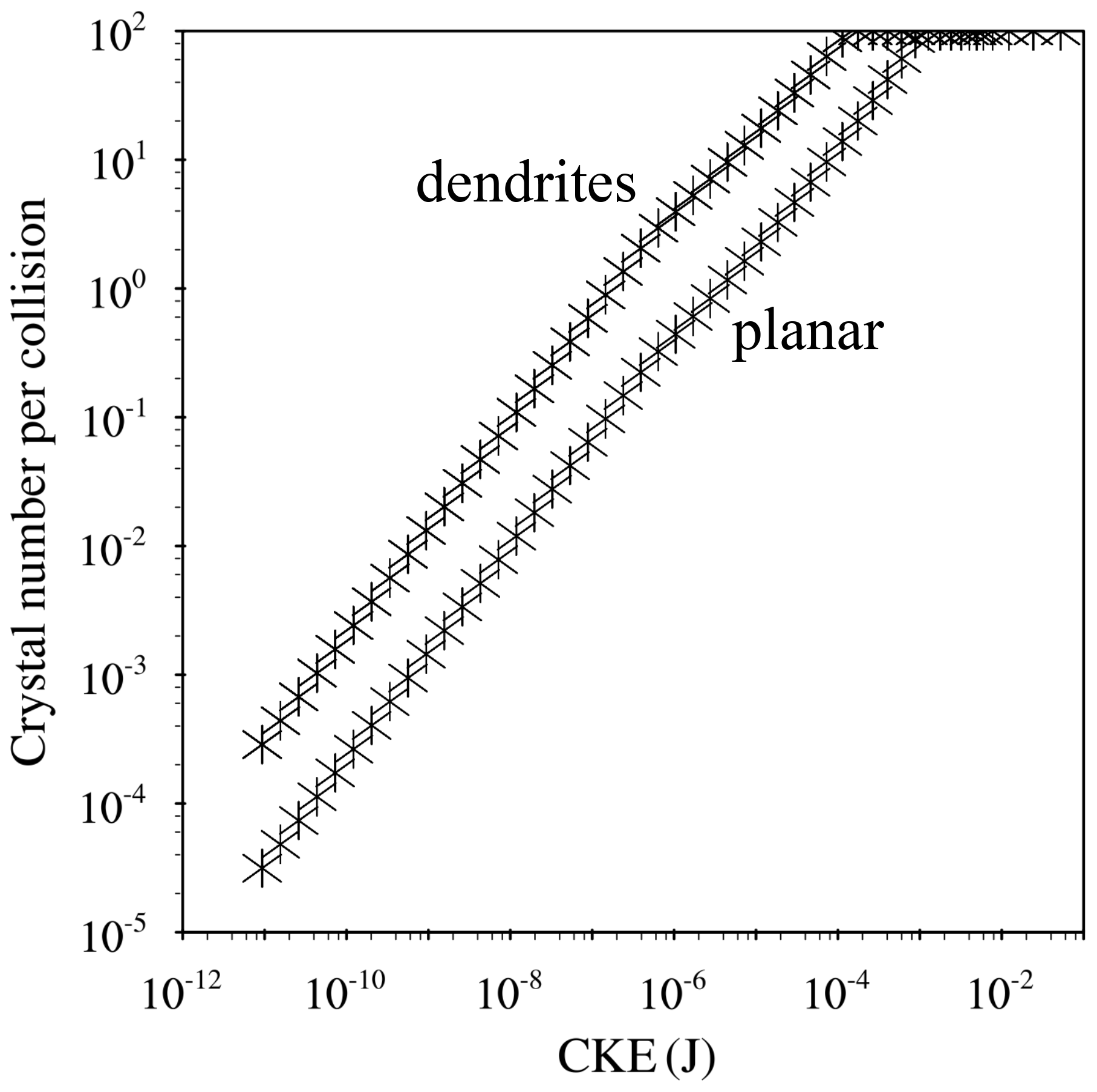
Figure 1 The number of fragments per collision as a function of initial collisional kinetic energy (CKE). The ice habit is assumed to be dendrites when the temperature (T) is between −12 and −17  ^∘C and is assumed to be spatial planar when $-\mathrm{40}{}^{\circ }\mathrm{C}<T<-\mathrm{17}{}^{\circ }\mathrm{C}$ and $-\mathrm{12}{}^{\circ }\mathrm{C}<T<-\mathrm{9}{}^{\circ }\mathrm{C}$, following Phillips et al. (2017a).

In this method, three types of collision are identified based on the type of collision particles: (1) cloud ice/snow collide with hail/graupel; (2) cloud ice/snow collide with cloud ice/snow; (3) hail/graupel collide with hail/graupel (not included currently, since CESM2-CAM6 does not treat graupel currently). For each collision type, different values of parameters α, A, C, and γ in Eq. (2) are yielded based on the measured relationship between fragment number and collisional kinetic energy (Phillips et al., 2017a).

Under the emulated bin framework, the new fragment production rate for each permutation of a bin is written as

$$\begin{array}{}\text{(4)}& N_{\text{iic}}=N{E}_{\mathrm{c}}\mathit{\delta }{N}_{\mathrm{1}}\mathit{\delta }{N}_{\mathrm{2}}\mathit{\pi }{\left(r_{\mathrm{1}}+r_{\mathrm{2}}\right)}^{\mathrm{2}}\left|v_{\mathrm{1}}-v_{\mathrm{2}}\right|,\end{array}$$

in which E_c is the accretion efficiency, assumed to be 0.5 to be consistent with the MG microphysics scheme, and δN₁ and δN₂ are the particle number concentrations in the two bins with particle sizes of r₁ and r₂, respectively.

The ice production rate for cloud ice mixing ratio is

$$\begin{array}{}\text{(5)}& P_{\text{iic}}=N_{\text{iic}}\mathit{\delta }{m}_{\text{ice}},\end{array}$$

in which δm_ice is mass for a single ice particle, prescribed as $\mathrm{2.09}\times {\mathrm{10}}^{-\mathrm{15}}$ kg.

2.2.3 Droplet shattering during rain freezing

Phillips et al. (2018) proposed numerical formulations for ice multiplication during the raindrop freezing. They suggested two modes of droplet breakup during the rain freezing based on the relative weight of raindrops and ice particles (Fig. 2).

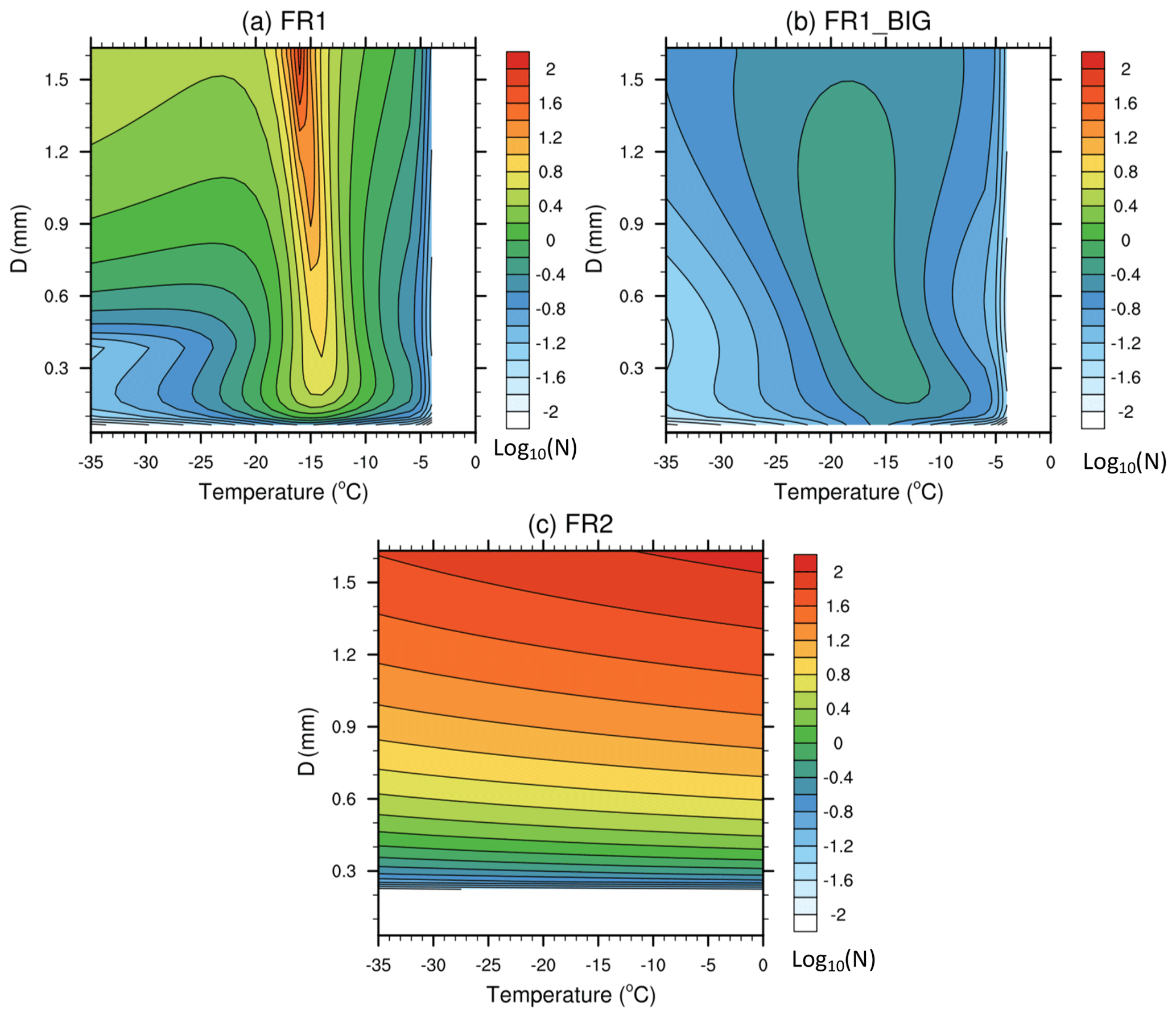
Figure 2 The number of fragments per frozen drop (shown as log ₁₀N) as a function of temperature and particle diameter, from (a) mode 1 of the rain freezing fragmentation (FR1), (b) mode 1 of the rain freezing fragmentation but for the big fragments (FR1_BIG), and (c) mode 2 of the rain freezing fragmentation (FR2).

In mode 1, the freezing of rain is triggered by a collision with less massive ice crystals or with INPs. By fitting to the laboratory data, Phillips et al. (2018) derived an empirical formulation for the number of ice fragments per frozen raindrop as a function of drop diameter and temperature. A Lorentzian distribution as a function of temperature was adopted to represent the number of ice fragments per frozen raindrop. There are two types of raindrop fragmentation: shattering to form “big” fragments and “tiny” splinters. The total (big plus tiny) and big ice fragments per frozen raindrop emitted in mode 1 of droplet shattering are given in Eqs. (6) and (7), respectively:

$$\begin{array}{}\text{(6)}& {\displaystyle }& {\displaystyle }{N}_{\mathrm{T}}=F\left(D\right)\mathrm{\Omega }\left(T\right)\left[{\displaystyle \frac{\mathit{\zeta }{\mathit{\eta }}^{\mathrm{2}}}{{\left(T-T_{\mathrm{0}}\right)}^{\mathrm{2}}+{\mathit{\eta }}^{\mathrm{2}}}}+\mathit{\beta }T\right]\text{(7)}& {\displaystyle }& {\displaystyle }{N}_{\mathrm{B}}=min\left\{F\left(D\right)\mathrm{\Omega }\left(T\right)\left[{\displaystyle \frac{{\mathit{\zeta }}_{\mathrm{B}}{\mathit{\eta }}_{\mathrm{B}}^{\mathrm{2}}}{{\left(T-T_{\text{B0}}\right)}^{\mathrm{2}}+{\mathit{\eta }}_{\mathrm{B}}^{\mathrm{2}}}}\right],N_{\mathrm{T}}\right\},\end{array}$$

where the parameters ζ, η, β, ζ_B, η_B, T₀, T_B0 are derived by fitting the formulations to a collection of laboratory data. Further details about empirical formulae can be found in Phillips et al. (2018). F(D) and Ω(T) are the interpolating functions for the onset of fragmentation, and T is the temperature in K. The mass of a big fragment is m_B=χ_Bm_rain, in which χ_B=0.4, and the mass of a small fragment is $m_{\mathrm{S}}=\frac{\mathit{\pi }{\mathit{\rho }}_i}{\mathrm{6}}{D}^{\mathrm{3}}$, in which ${\mathit{\rho }}_i=\mathrm{500}\mathrm{kg}{\mathrm{m}}^{-\mathrm{3}}$.

The observational data used for the formulations of raindrop freezing by mode 1 were limited to a drop diameter of 1.6 mm and a temperature range between −4 and −25 ^∘C. Phillips et al. (2018) linearly extrapolated their algorithm for larger particles and other temperatures in the mixed-phase cloud regime. As shown in Fig. 2a and b, mode 1 of the droplet shattering is most effective near −15^∘.

In mode 2, a theoretical approach is adopted which is based on the assumption that the number of fragments generated when a drop collides with a more massive ice particle is controlled by the initial kinetic energy and surface energy (Fig. 2c). The number of fragments generated per frozen drop in mode 2 is given as

$$\begin{array}{}\text{(8)}& N_{\text{fr2}}=\mathrm{3}\mathrm{\Phi }\left(T\right)\times \left[\mathrm{1}-f\left(T\right)\right]\times max(\text{DE}-{\text{DE}}_{\mathrm{c}}),\end{array}$$

where DE is the dimensionless energy and is expressed as

$$\begin{array}{}\text{(9)}& \text{DE}={\displaystyle \frac{k_{\mathrm{0}}}{S_{\mathrm{e}}}},\end{array}$$

where k₀ is the initial kinetic energy, which is given in Eq. (3), S_e is the surface energy, expressed as S_e=γ_liqπD² (for D>150 µm), and γ_liq is the surface tension of liquid water, which is 0.073 J m⁻². DE_c in Eq. (8) is set to be 0.2. f(T) is the frozen fraction (Phillips et al., 2018) and is given as

$$\begin{array}{}\text{(10)}& f\left(T\right)={\displaystyle \frac{-C_{\mathrm{w}}T}{L_{\mathrm{f}}}}.\end{array}$$

where C_w is the specific heat capacity of liquid water (4200 $\mathrm{J}{\mathrm{kg}}^{-\mathrm{1}}{\mathrm{K}}^{-\mathrm{1}}$), and L_f is the specific latent heat of freezing (3.3×10⁵ J kg⁻¹), Φ(T)=0.5 at −1 ^∘C and $\mathrm{\Phi }\left(T\right)=min\left[\mathrm{4}f\left(T\right),\mathrm{1}\right]$.

2.2.4 Rime splintering

The MG microphysics already includes the SIP associated with rime splintering, which is also known as the Hallett–Mossop (HM) process. In this process, secondary ice particles are generated during the accretion of cloud droplets by snow, and a part of rimed mass is converted to cloud ice. The ice number production rate is based on the parameterization of Cotton et al. (1986), which is given as

$$\begin{array}{}\text{(11)}& N_{\text{HM}}=C_{\text{sip\_HM}}\times p_{\text{sacws}},\end{array}$$

where p_sacws is the riming rate of cloud droplets by snow and is expressed as

$$\begin{array}{}\text{(12)}& p_{\text{sacws}}={\displaystyle \frac{\mathit{\pi }\times a_{\text{vs}}\times \mathit{\rho }\times N_{\text{0s}}\times E_{\text{ci}}\times \mathrm{\Gamma }(b_{\text{vs}}+\mathrm{3})}{\mathrm{4}\times {\mathit{\lambda }}^{b_{\text{vs}}+\mathrm{3}}}},\end{array}$$

in which E_ci is the collection efficiency for the riming of cloud droplets by snow, a_vs and b_vs are the fall speed parameters for snow particles, b_vs=0.41, and $a_{\text{vs}}=\mathrm{11.72}\times \frac{{\mathit{\rho }}_{\mathrm{850}}}{\mathit{\rho }}$, ρ and ρ₈₅₀ are air density and typical air density at 850 hPa, respectively, and N_0s and λ are the parameters for the snow particle size distribution.

The conversion coefficient C_{sip_HM} in Eq. (11) depends on temperature T_c in degrees Celsius (^∘C):

$$\begin{array}{}\text{(13)}& \begin{array}{rl}{C}_{\text{sip\_HM}}& ={\displaystyle \frac{\mathrm{3.5}\times {\mathrm{10}}^{\mathrm{8}}\times (-\mathrm{3}-T)}{\mathrm{2}}},\\ & \text{when}-\mathrm{5}<T_{\mathrm{c}}<-\mathrm{3},\end{array}\end{array}$$

and

$$\begin{array}{}\text{(14)}& \begin{array}{rl}{C}_{\text{sip\_HM}}& ={\displaystyle \frac{\mathrm{3.5}\times {\mathrm{10}}^{\mathrm{8}}\times (T-(-\mathrm{8}\left)\right)}{\mathrm{3}}},\\ & \text{when}-\mathrm{8}<T_{\mathrm{c}}<-\mathrm{5}.\end{array}\end{array}$$

The production rate for cloud ice mixing ratio is given as

$$\begin{array}{}\text{(15)}& P_{\text{HM}}=N_{\text{HM}}\mathit{\delta }{m}_{\text{ice}},\end{array}$$

in which δm_ice is mass for a single ice particle in the HM process, prescribed as $\mathrm{2.09}\times {\mathrm{10}}^{-\mathrm{15}}$ kg. The rime splintering rate as a function of p_sacws and temperature is shown in Fig. 3.

3 Case description, observations, and model experiments

3.1 M-PACE case

In this study, we focus on the Arctic mixed-phase clouds observed during the Department of Energy (DOE)'s Atmospheric Radiation Measurement (ARM) Mixed-Phase Arctic Cloud Experiment (M-PACE). The M-PACE campaign was conducted over the North Slope of Alaska (NSA) during the autumn from 27 September to 22 October 2004.

Various types of clouds were observed during M-PACE, including multilayer, boundary-layer mixed-phase stratus, cirrus, and altostratus clouds associated with the frontal system (Verlinde et al., 2007; Liu et al., 2007, 2011; Xie et al., 2008). Single-layer mixed-phase clouds were formed under moderately supercooled conditions, with the cloud temperature at around −10 ^∘C (Verlinde et al., 2007; McFarquhar et al., 2007), providing a favorable condition for studying the influence of SIP on cloud evolution (Field et al., 2016).

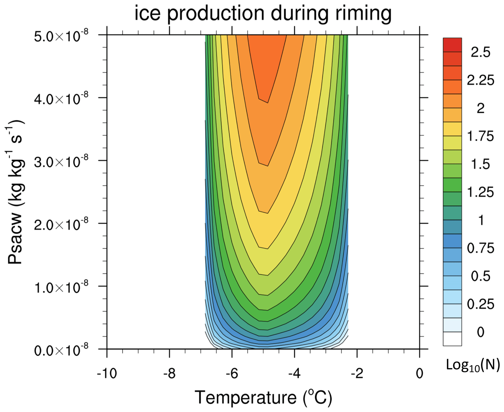
Figure 3 The rime splintering rate (shown as log ₁₀N) as a function of temperature and riming rate.

The synoptic-scale systems regulated the properties of clouds observed during the M-PACE campaign. Hence, Verlinde et al. (2007) divided the M-PACE period into three synoptic regimes and two transition periods based on the synoptic weather conditions. The first synoptic regime began on 24 September and lasted until 1 October 2004, when a well-developed trough dominated aloft with several low-pressure systems that influenced the surface. Followed by the first transition period between 2 and 3 October, the second synoptic regime occurred between 4 and 14 October (Fig. 4), which was controlled by a pronounced high-pressure system. The second transition period was from 15–17 October. By 18 October, a fast-developing strong frontal system controlled the cloud formation over the NSA in the third synoptic regime (Fig. 4). During M-PACE, the surface flux of water vapor, sensible heat, and latent heat played different roles in the cloud formation. For example, clouds formed in response to a strong surface forcing during the second regime, while clouds formed under a relatively weak surface forcing during the third regime. In this study, we evaluate the modeled cloud properties with M-PACE observations in the second and third synoptic regimes, focusing on the boundary-layer mixed-phase stratus during 9–12 October in the second regime.

Figure 4 Temporal evolution of (a) LWP, (b) IWP from remote sensing retrievals shown by different markers, CTL experiment (solid orange line) and SIP_PHIL experiment (solid dark green line), and (c) observed time–pressure cross section of the cloud fraction. The shadings show the multilayer stratus, single-layer stratus, transition, and frontal periods.

3.2 Observation data

The observed cloud occurrence data at Utqiaġvik (formerly Barrow, located at 71.3^∘ N, 156.6^∘ W) are from the ARM Climate Modeling Best Estimate product (Xie et al., 2010). The liquid water path (LWP) and ice water path (IWP) data are obtained from Zhao et al. (2012). Specifically, Shupe and Turner's data are based on the retrievals of cloud properties measured by the ARM Millimeter-Wavelength Cloud Radar (Shupe et al., 2005) and the Microwave Radiometer (MWR) (Turner et al., 2007), with the uncertainties for liquid water content (LWC) within 50 % and for ice water content (IWC) within a factor of 2. For Wang's data, IWP is retrieved from the combined ARM Millimeter-Wavelength Cloud Radar and Micropulse lidar measurements (Wang and Sassen, 2002) with an uncertainty of 35 % (Khanal and Wang, 2015). LWP is retrieved from the ARM MWR measurements with an uncertainty of 50 % (Wang, 2007). For Deng's data, IWC is retrieved based on the Millimeter-Wavelength Cloud Radar measurements, with a retrieval error within 85 % (Deng and Mace, 2006). For Dong's data, LWC is retrieved from the MWR measurements with an uncertainty within 113 % (Dong and Mace, 2003). Note that measured IWC and IWP cannot distinguish cloud ice from the snow. The simulated IWP and IWC therefore include the snow component, which is consistent with observations used in this study.

The ICNC was measured during the M-PACE single-layer mixed-phase stratus period. The data include 53 profiles measured in four flights over Utqiaġvik (formerly Barrow) and Oliktok Point (located at 70.5^∘ N, 149.9^∘ W) by the University of North Dakota Citation aircraft. By combining measurements from different probes, McFarquhar et al. (2007) provided cloud particle size distributions over a continuous size range. The forward scattering spectrometer probe (FSSP) measured particle number concentrations with particle diameters between 3 and 53 µm, while the one-dimensional cloud probe (1DC) counted cloud particles ranging from 20 to 620 µm. The two-dimensional cloud probe (2DC) covered particle sizes from 30 to 960 µm, while the high-volume precipitation sampler (HVPS) sampled particles from 0.4 to 40 mm. The data were collected every 10 s but were averaged to 30 s⁻¹ to ensure adequate statistical sampling. The cloud phase was identified by detecting the presence of supercooled droplets by the Rosemount Icing Detector (RICE). In mixed-phase clouds, any particles larger than 125 µm are identified as ice particles, and cloud particles smaller than 53 µm are counted as liquid-phase particles. Particles with a diameter ranging from 53 to 125 µm are counted as a liquid when there is drizzle and as ice if there is no drizzle. A more detailed description of the particle-phase identification algorithm can be found in McFarquhar et al. (2007). When comparing the simulated ICNC with the observations, we only consider ice particles larger than 53 µm, as the observations were limited to ice particles larger than 53 µm.

However, the M-PACE data were collected before the advent of shatter mitigating tips and before algorithms for removing the shattered particles had been developed. Thus, there are no corrections for the shattering effect in these data. Previous studies indicated an averaged reduction of ice number concentrations by 1–4.5 times and up to a factor of 10 (for some data samples) in other field campaigns, such as the Instrumentation Development and Education in Airborne Science 2011 (IDEAS-2011), the Holographic Detector for Clouds (HOLODEC), and the Indirect and Semidirect Aerosol Campaign (ISDAC), which also used the 2DC cloud probe but adopted anti-shattering tips and algorithms for removing the shattered particles (Jackson and McFarquhar, 2014; Jackson et al., 2014). In order to account for the anti-shattering effect, observed ice number concentrations were scaled by a factor of $\mathrm{1}/\mathrm{4}$ and $\mathrm{1}/\mathrm{2}$, respectively, to consider the possible range of the shattering effect. Furthermore, to be consistent with Fig. 10 in Jackson et al. (2014), only ice particles with diameters larger than 100 µm are included in our model and observation intercomparisons.

3.3 Model setup and description of model experiments

In this study, we run SCAM with 32 vertical layers from the surface up to 3 hPa. The model is initialized and driven by the large-scale forcing data every 3 h. The forcing data developed by Xie et al. (2006) include the divergence and advection of moisture and temperature as well as the surface flux. The simulation period is from 5 to 22 October 2004 and covers the second and third synoptic regimes and the transition period between them.

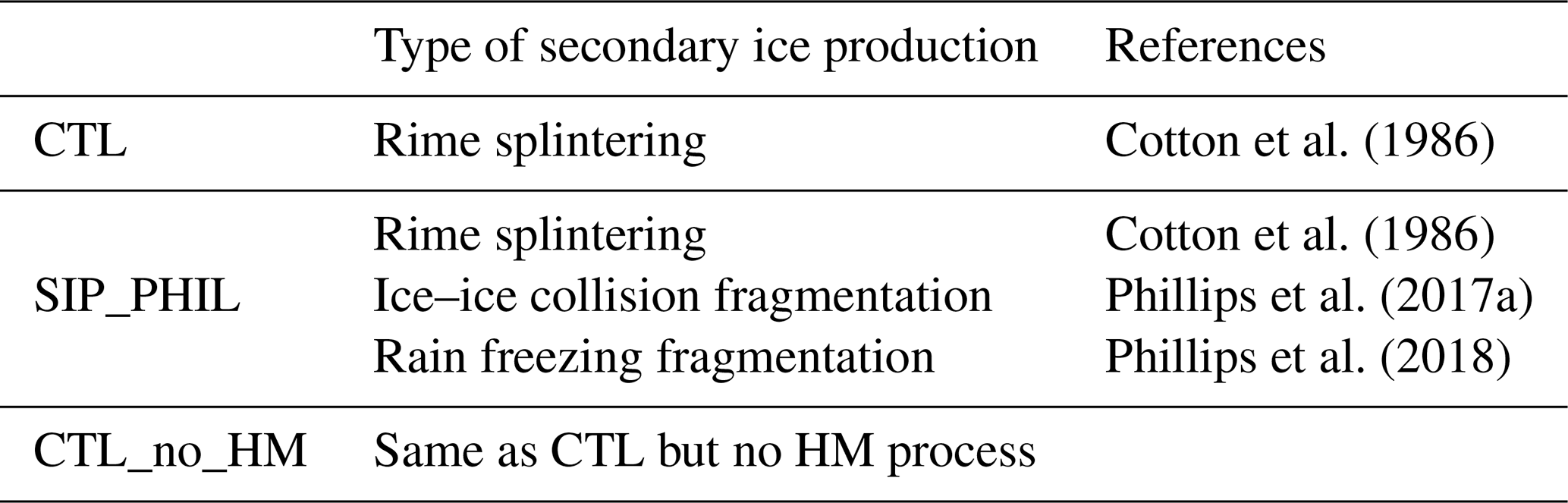
A detailed description of model experiments along with SIP mechanisms in these experiments is provided in Table 1. The control experiment (CTL) uses the default CAM6 model that only includes the SIP due to the HM process. The impacts of two new SIP mechanisms, including the ice–ice collision breakup and rain freezing fragmentation, based on Phillips et al. (2017a, 2018) are addressed in the SIP_PHIL experiment. To examine the impact of rime splintering in the CTL experiment, we conducted the CTL_no_HM experiment that is similar to CTL but without the HM process.

Table 1 List of experiments.

4 Results

4.1 SIP impacts on different types of clouds during M-PACE

Figure 4 shows the temporal evolution of LWP, IWP, and cloud fractions from two model simulations (CTL and SIP_PHIL) and their comparison to observations. The model simulations cover the second and third synoptic regimes as well as the transition period between them. Two different types of clouds were formed in response to the strong surface forcing during the second synoptic regime from 4 to 14 October. As shown in Fig. 4c, multilayer stratus occurred from 5 to 8 October, and the clouds extended from 950 up to 500 hPa. Between 9 and 14 October, single-layer boundary-layer stratus occurred between 800 and 950 hPa. Because of the dramatic change in cloud types in the second regime, we further separate the second regime into two time periods. Then, we select typical days in the four time periods for our analysis in this study, as shown in Fig. 4. The period from 6 to 8 October is selected as the “multilayer stratus” period. The period from 9 to 12 October is selected as the “single-layer stratus” period, followed by the transition period marked on 16 October. The period between 18 and 20 October is selected to represent the “frontal cloud” type during the third regime.

Figure 4 shows that the simulated IWP is systematically underestimated during M-PACE in the CTL experiment. The maximum value of IWP in CTL is smaller than 50 g m⁻² during M-PACE but up to 500 g m⁻² in the measurements. The SIP_PHIL experiment shows decreased LWP and increased IWP compared with CTL, reaching a better agreement with the measurements. For example, IWP increases from 50 g m⁻² in CTL to 425 g m⁻² in SIP_PHIL on 20 October, compared with 300∼475 g m⁻² from different measurements (Fig. 4). The simulated LWP is overestimated during the multilayer stratus, the second half of the single-stratus, and the frontal cloud period in CTL, particularly on 20 October. The SIP_PHIL experiment decreases the LWP from 550 g m⁻² in CTL to 300 g m⁻² on 11 October and from 425 g m⁻² in CTL to 70 g m⁻² on 20 October (Fig. 4a). The CTL_no_HM experiment has similar results to the CTL experiment.

During the multilayer stratus period, the CTL and SIP_PHIL experiments show that the cloud top is located at about 5 km with a temperature of −20 ^∘C (Fig. 5). These cloud properties are consistent with the observations (Verlinde et al., 2007) that show a minimum observed cloud temperature of −17 ^∘C (Fig. 4). However, we notice a significant overestimation of cloud amount at 6–8 km on 7 October by the model simulations in Fig. 5, as compared to the observation in Fig. 4c.

Figure 5 Time–height cross section of cloud fraction (first column), LWC (second column), IWC (third column), and ice crystal number concentration (fourth column) from CTL (first row) and SIP_PHIL (second row) and the differences between SIP_PHIL and CTL (SIP_PHIL minus CTL, third row).

During this period, IWC is increased in the SIP_PHIL experiment compared to CTL, while LWC is decreased. The mean vertical profiles of simulated IWC and LWC in this period are shown in Fig. 6. The simulated values of LWC and IWC are lower than observations, particularly for IWC. LWC decreases from 130 mg m⁻³ in CTL to 80 mg m⁻³ in SIP_PHIL below 1 km. IWC increases from 3 mg m⁻³ in CTL to 5 mg m⁻³ in SIP_PHIL. The time-averaged IWP increases from 11.2 g m⁻² in CTL to 17.1 g m⁻² in SIP_PHIL but is still lower than the observed value of 55.6 g m⁻² (Table 2). After considering the SIP in the model, for the multilayer stratus period, ICNC is increased by 1 L⁻¹ (Fig. 5) at an altitude of 1 to 4 km. Observations of ICNC are not available during this period.

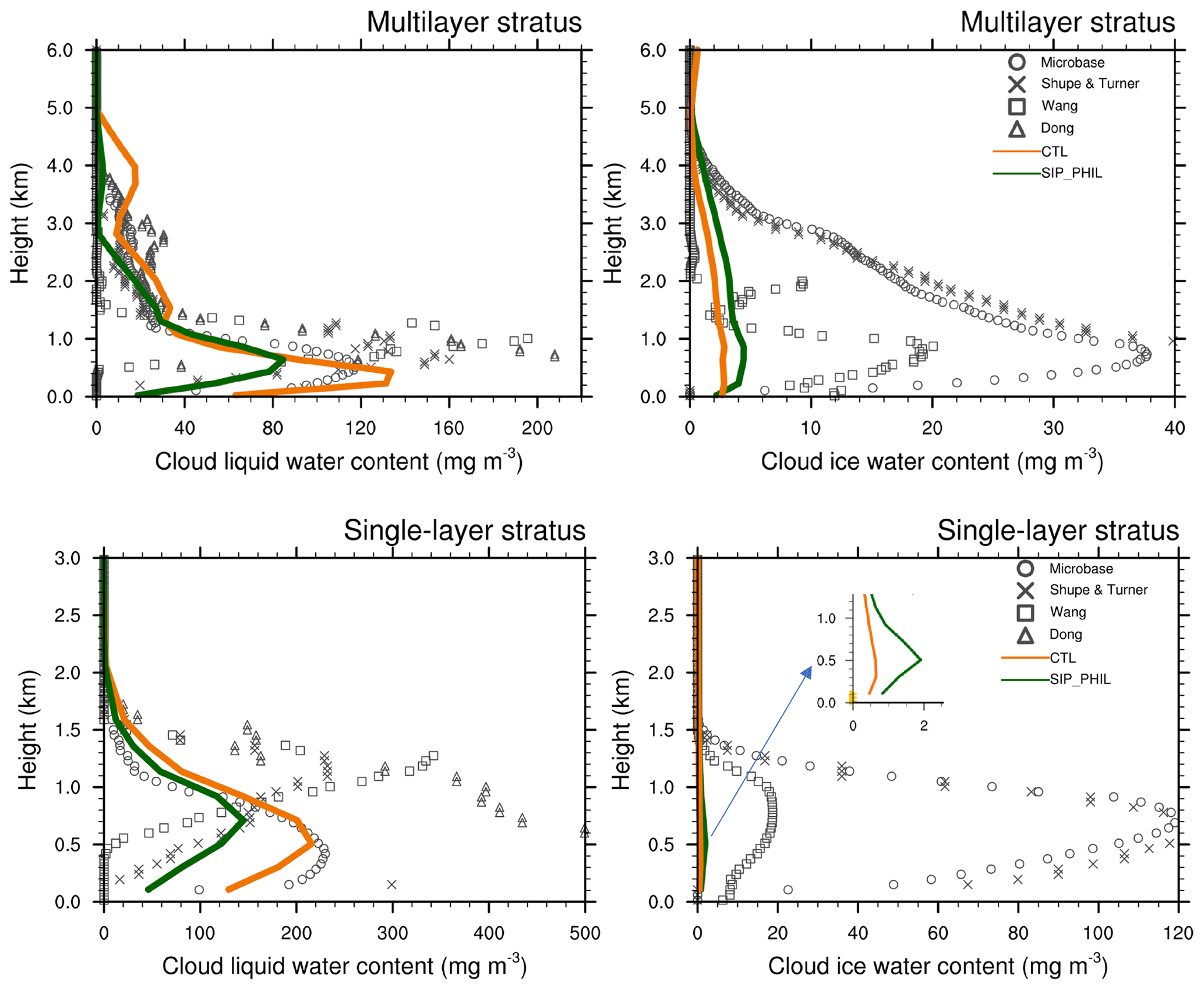
Figure 6 Vertical profiles of IWC and LWC during multilayer stratus and single-layer stratus periods from remote sensing retrievals shown by different markers, CTL experiment (solid orange line) and SIP_PHIL experiment (solid dark green line).

Table 2 The temporally averaged IWP, LWP (unit: g m⁻²), and vertically integrated ice crystal number concentration (unit: m⁻²) during the four periods from observations (OBS) and CTL, CTL_no_HM, and SIP_PHIL experiments.

Between 9 and 14 October, a persistent boundary-layer mixed-phase stratus occurred between 800 and 950 hPa, with the cloud top temperature at around −15 ^∘C (Verlinde et al., 2007). This single-layer stratus was separated from the surface based on the measurement (Fig. 4c). However, modeled clouds extend to the surface in CTL (Fig. 5). This bias is alleviated in SIP_PHIL on 8 and 11 October (Fig. 5). Previous studies also found that this bias partially results from the overestimation of low-level moisture in the large-scale forcing data (Zhang et al., 2019, 2020).

Observed cloud liquid is located above the cloud ice during this period, with the LWC peak ∼0.5 km above the IWC peak. Observed vertical profile of LWC shows a maximum of 300 mg m⁻³ (ranging from 210 to 500 mg m⁻³) at ∼1.25 km, while observed IWC peaks at 0.75 km (Fig. 6). This characteristic is clearly captured by the SIP_PHIL experiment, with the peaks of LWC and IWC located at 0.75 and 0.5 km, respectively (Fig. 6). A better relative position of cloud liquid and ice in SIP_PHIL indicates a better simulation of interactions between cloud physics and dynamics. This distinct feature also contributes to the longevity of mixed-phase clouds in the Arctic, as discussed in Sect. 1. In SIP_PHIL, the maximum IWC value is 4 times larger than that in CTL (2 versus 0.5 mg m⁻³); accordingly, temporally averaged IWP increases from 0.9 in CTL to 2.5 g m⁻² in SIP_PHIL (Table 2). Meanwhile, ICNC in SIP_PHIL is higher than that in CTL, and the maximum ICNC goes up by 5 L⁻¹ at 0.5 km on 11 October (Fig. 5). Thus, SIP adds an extra source of ice crystals to the boundary-layer mixed-phase stratus clouds.

During the transition period, several distinct liquid layers are interrupted by the ice enriched layers in the observation. Due to the coarse vertical resolution, the model may not be able to capture this vertical variation accurately. Considerable variation was noticed in the observed IWC, with a maximum IWC of 0.8–1.8 mg m⁻³ (Fig. 7). The CTL experiment substantially underestimates IWC, as it produces IWC less than 0.1 mg m⁻³. The maximum IWC in SIP_PHIL is 1.15 mg m⁻³, providing a better agreement with the observation. The simulated peak LWC is decreased from 80 mg m⁻³ in CTL to 65 mg m⁻³ in SIP_PHIL, which is closer to the observed value of 55 mg m⁻³. The temporally averaged IWP in SIP_PHIL is 10⁴ times larger than that in CTL, with values of 0.0001, 3.6, and 5.6 g m⁻² in CTL, SIP_PHIL, and observations, respectively (Table 2). The vertically integrated ICNC is 7.66 and 4.57×10⁵ L⁻¹ in CTL and SIP_PHIL, respectively (Table 2). Considering SIP in the model increases vertically integrated ICNC by 5 orders of magnitude during the transition period.

During the frontal cloud period, stratocumulus and altostratus clouds associated with the frontal system extended from the surface up to 8 km (Fig. 4). The SIP_PHIL experiment shows the largest absolute increases in IWC and ICNC compared to the other periods (Fig. 5). The peak of modeled IWC is located at 2.5 km, with values of 2 and 8 mg m⁻³ in CTL and SIP_PHIL, respectively (Fig. 7), much lower than the observation (ranging from 8 to 40 mg m⁻³). IWP is 10.4, 26.1, and 96 g m⁻² in CTL, SIP_PHIL, and the observations, respectively (Table 2). ICNC is increased by up to 7 L⁻¹ between 2 and 4 km on 20 October from CTL to SIP_PHIL (Fig. 5). The simulated LWP is decreased from 127.6 to 41.2 g m⁻², which is closer to the observed value of 50.2 g m⁻².

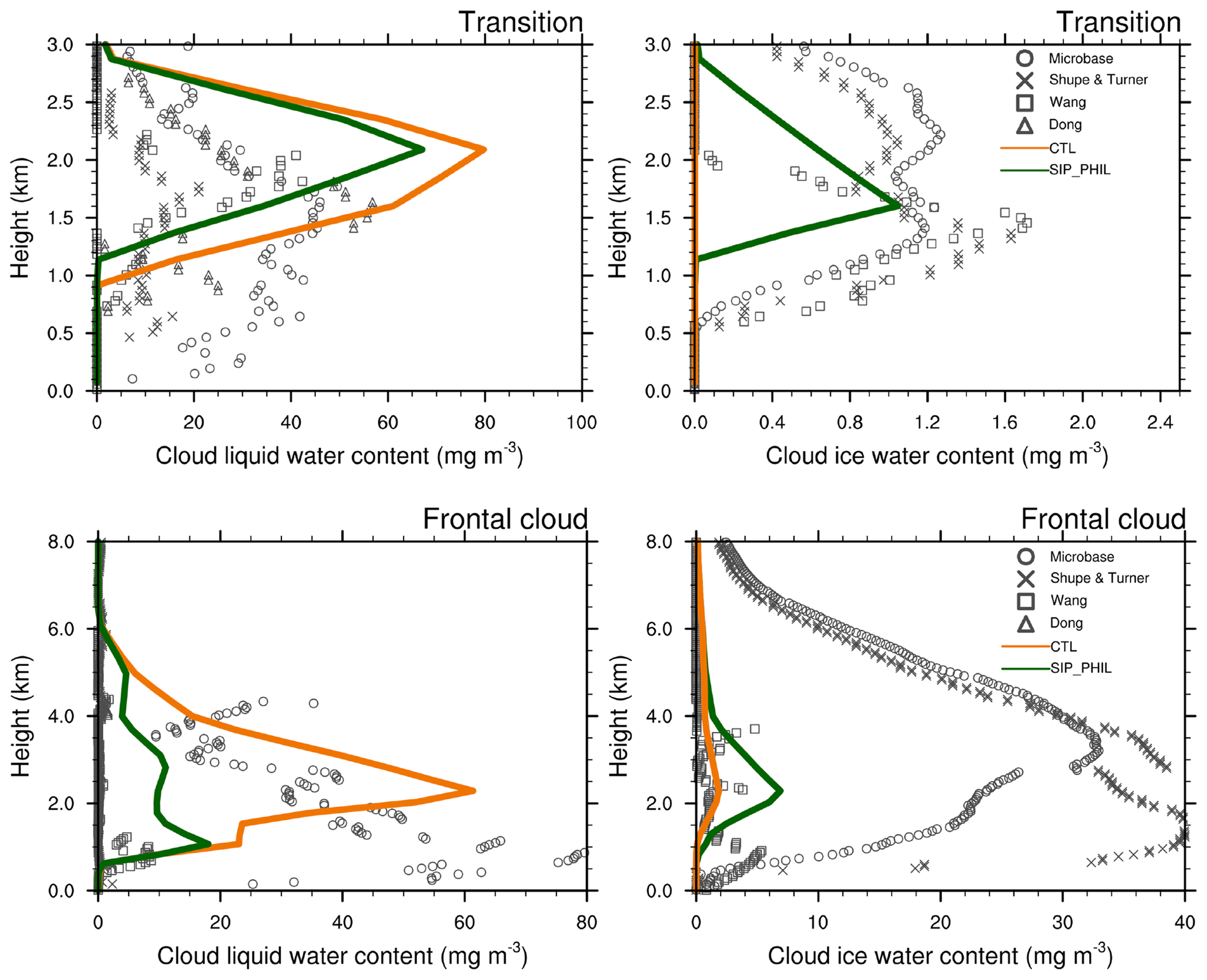
Figure 7 Vertical profiles of IWC and LWC during the transition and frontal cloud periods, from remote sensing retrievals shown by different markers, CTL experiment (solid orange line) and SIP_PHIL experiment (solid dark green line).

The relative importance of primary and secondary ice production is shown as pie charts in Fig. 8, to identify the dominant ice production mechanism in different types of the Arctic clouds. The primary ice production (i.e., ice nucleation) is more important in the clouds with colder cloud tops, such as multilayer stratus and frontal clouds, with cloud top temperatures colder than −25 and −40 ^∘C, respectively. The primary ice production contributes 37 % and 69 % to the total ice production during the multilayer stratus and frontal cloud periods, respectively. Primary ice production is more efficient in deep clouds due to the inverse relationship between the ice nucleation rate and temperature. SIP is more important than primary ice production in the boundary-layer stratus and in clouds during the transition period when cloud top temperatures were at −15 ^∘C. The fragmentation of freezing raindrops contributes the most (up to 80 %) to the ice production in the single-layer boundary-layer stratus. The breakup from ice–ice collisions contributes 22 % to the total ice production in the frontal clouds, while the rime splintering contributes 22 % to the multilayer stratus. These two SIP mechanisms (i.e., breakup from ice–ice collisions and rime splintering) account for a small fraction of the ice production in the boundary-layer stratus.

Figure 8 Pie charts showing the relative contributions to total ice production from primary production (i.e., ice nucleation), rime splintering (HM), fragmentation of frozen rain (including the small fragments in the first mode (FR1), big fragments in the first mode (FRB), and the second mode (FR2)), breakup from ice–ice collisions (including snow and cloud ice collision (ISC) and snow and snow collision (SSC)). During the four M-PACE periods, the vertically integrated process rates are used in the plot.

Next, we will focus on the SIP impacts on the boundary-layer stratus related to the phase partitioning (Sect. 4.2) and ICNC (Sect. 4.3).

4.2 SIP impact on occurrence and phase partitioning of the mixed-phase clouds

Figure 9 shows the liquid fraction (defined as $\text{LWC}/(\text{LWC}+\text{IWC})$ as a function of normalized height in the single-layer boundary-layer stratus. The normalized height Z_n is 0 at cloud base and 1 at cloud top. IWC from the model includes all the ice hydrometeors to compare it with observations. Figure 9a reveals two features of the observed single-layer boundary-layer clouds: (1) mixed phase is dominant in the clouds, and (2) the liquid fraction increases with cloud altitude. The liquid fraction is between 0.05 and 0.95 in most portions of the clouds, indicating a mixed-phase feature in the observation. In the upper portion of the clouds, the observed liquid fraction is larger than 0.6, with the mean value increasing with height. In the lower portion of the clouds, the ice mass fraction increases as a result of ice growth by riming of cloud liquid and ice sedimentation from the upper levels. The CTL experiment cannot reproduce the observed mixed-phase feature. A large portion of the clouds is in liquid phase, with the liquid fraction close to 1 in CTL, which significantly overestimates the liquid fraction in the clouds. This is vastly different from previous versions of CAM. CAM5 showed an underestimation of the liquid fraction (Liu et al., 2011; Cesana et al., 2015; Tan and Storelvmo, 2016, 2019; Zhang et al., 2019), while CAM3 showed a decrease of the liquid fraction with height due to its use of a temperature-dependent phase partitioning (Liu et al., 2007).

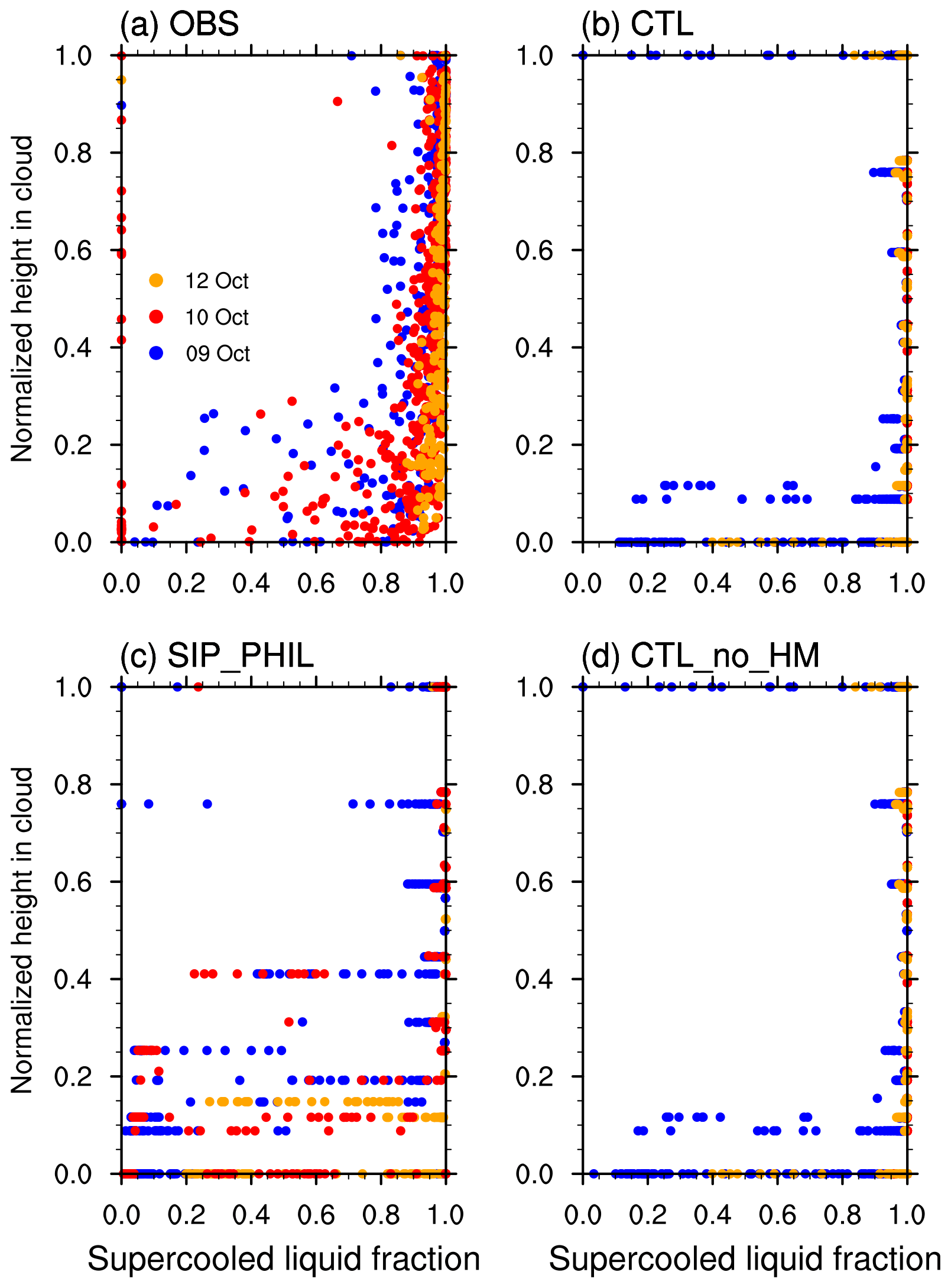
Figure 9 Liquid fraction as a function of normalized cloud height from cloud base. The normalized cloud altitude Z_n is defined as $Z_{\mathrm{n}}=\left(z-Z_{\mathrm{b}}\right)/\left(Z_{\mathrm{t}}-Z_{\mathrm{b}}\right)$, in which z is the altitude, Z_b is the altitude of cloud base, and Z_t is the altitude of cloud top, from (a) observations, (b) CTL, (c) SIP_PHIL, and (d) CTL_no_HM.

The SIP_PHIL experiment improves the model simulation of cloud phase, with an increased ice fraction in the bottom half of the clouds by adding an extra source of ice crystals from SIP (Fig. 9c). The CTL_no_HM experiment gives very similar results to the CTL experiment (Fig. 9d). Note that the modeled liquid fraction is distributed on discrete vertical levels (Fig. 9b–d) due to the coarse model vertical resolution (with only 10 vertical levels below 2 km). In contrast, observed data were detected at 10 s⁻¹ resolution during spiral ascents and descents in the clouds so that the observed liquid fraction is distributed continuously with height.

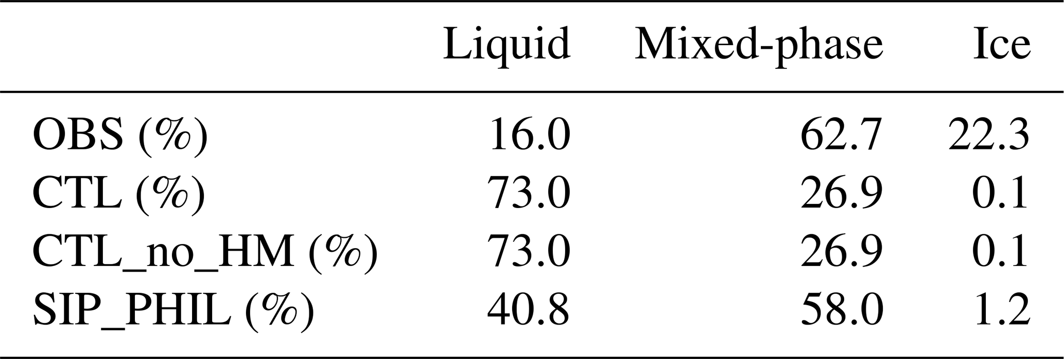
For the cloud occurrence, 62.7 % of observed clouds are mixed-phase, and only 16 % are liquid phase during the single-layer stratus period, as shown in Table 3. The liquid-phase cloud occurrence is 73 % in CTL and only 26.9 % for mixed-phase clouds, indicating too much liquid-phase and too little mixed-phase occurrence in CAM6. The mixed-phase cloud occurrence is 58.8 % in SIP_PHIL and agrees much better with the observation. Thus, there are more frequent mixed-phase clouds in SIP_PHIL. However, the occurrence of ice phase is still underestimated, and that of the liquid phase overestimated in SIP_PHIL. Note that we define the modeled clouds with a total cloud water amount larger than 0.001 g m⁻³ and a liquid fraction between 0.5 % and 99.5 % as mixed-phase clouds, which is consistent with the observations (McFarquhar et al., 2007).

Table 3 Percentage of occurrence of liquid, mixed-phase, and ice clouds during single layer mixed-phase clouds from observations (OBS) and CTL, CTL_no_HM, and SIP_PHIL experiments.

4.3 SIP impact on ice crystal number concentration

4.3.1 Vertical distribution of ice crystal number concentration

The vertical distribution of ICNCs in the single-layer boundary-layer stratus clouds on 9, 10, and 11 October from model simulations and observations is shown in Fig. 10. The measured ICNCs when applied with a correction factor of $\mathrm{1}/\mathrm{4}$ range from 0.02 to 20 L⁻¹, with an average value of 1 L⁻¹. The CTL and CTL_no_HM experiments have similar results, and both underestimate the ICNCs in all the cloud layers, with a mean ICNC of ∼0.1 L⁻¹ and a maximum concentration of 1 L⁻¹. The mean ICNC is increased to ∼1 L⁻¹ in the SIP_PHIL experiment, with a maximum concentration of 30 L⁻¹, which is in better agreement with the observations compared to CTL. ICNCs are increased by more than 1 order of magnitude in the lower portion of the clouds, although they are still lower than those observed in the upper portion of the clouds.

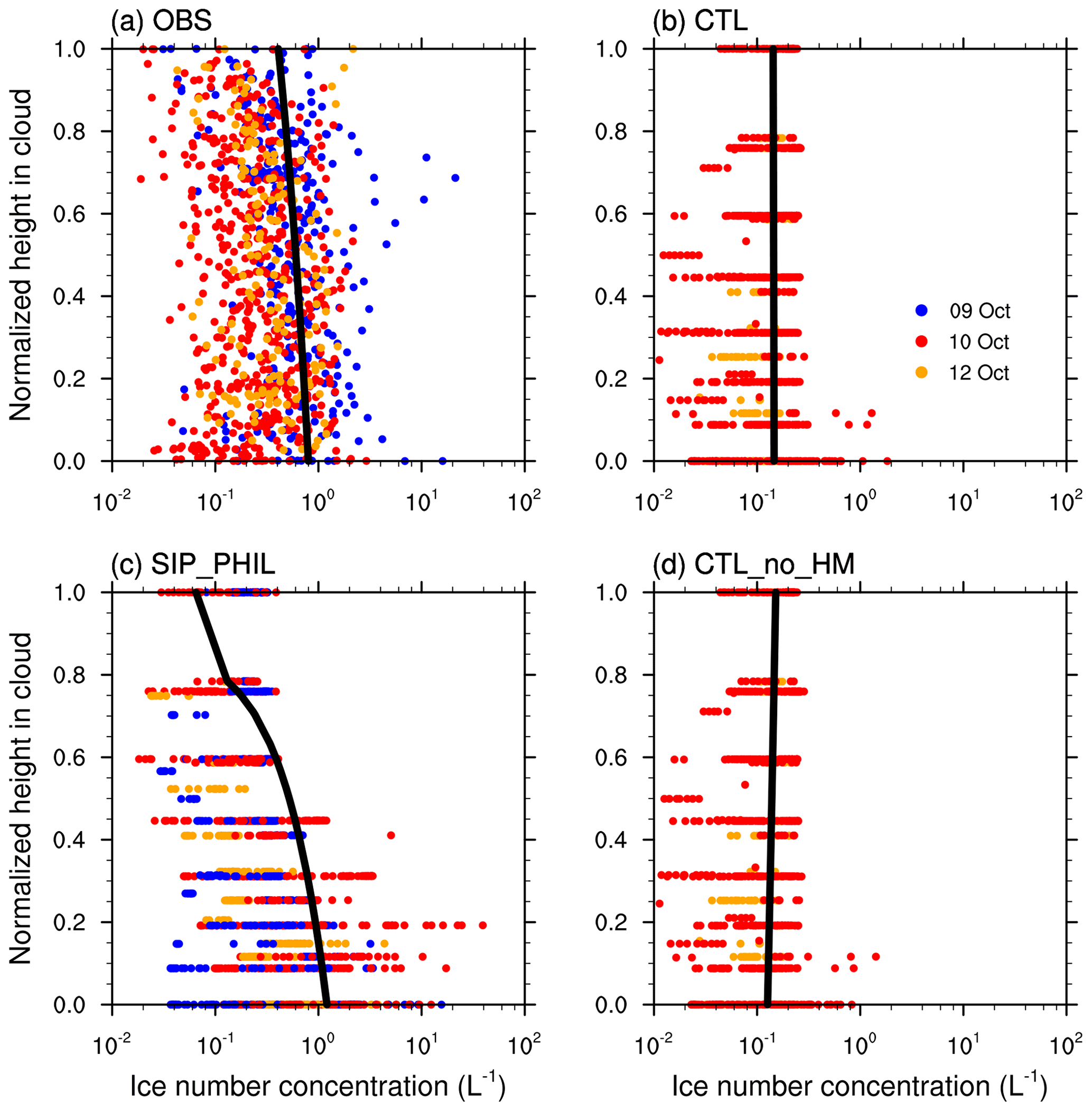
Figure 10 Ice number concentrations as a function of normalized cloud height from cloud base from (a) observations, (b) CTL, (c) SIP_ PHIL, and (d) CTL_no_HM. Solid black lines show the linear regression between ice number concentration and height. Only ice particles with diameters larger than 100 µm from observations and model simulations are included in the comparison. A correction factor of $\mathrm{1}/\mathrm{4}$ is applied to the observed ice number concentrations shown in (a) based on Jackson and McFarquhar (2014) and Jackson et al. (2014).

Figure 10 also shows the linear regressions of ICNCs as a function of cloud altitude (black lines). ICNCs increase towards the cloud base in the observation, revealing ice multiplication during the ice growth and sedimentation. The CTL experiment shows that the ICNCs decrease towards the cloud base, an opposite pattern compared to the observation. SIP_PHIL captures the observed pattern in the vertical profile of ICNCs (Fig. 10c), suggesting that SIP is an important source of ice crystals near the cloud base in the Arctic boundary-layer mixed-phase stratus. Furthermore, the vertical distribution of ice particles is important for the longevity of the Arctic mixed-phase clouds, which features lower ICNCs in the upper portion of clouds and higher ICNCs towards the cloud base.

4.3.2 PDF of ice crystal number concentration

Figure 11 shows the probability density function (PDF) (i.e., the frequency of occurrence) of ICNCs from model simulations and observations for the boundary-layer mixed-phase stratus period (9–12 October 2004). Note that only particles with a diameter greater than 100 µm are included in the observed and modeled ICNCs. The PDF distribution in SIP_PHIL shows a shift to the right, with the ICNC peak much closer to the observations than CTL. The median ICNC is 0.13 L⁻¹ in CTL, shifting to 0.27 L⁻¹ in SIP_PHIL, which is closer to the observed median value of 0.32 L⁻¹.

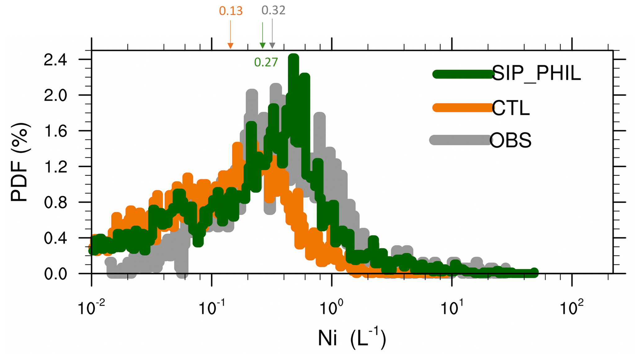
Figure 11 The probability density function (PDF) of ice crystal number concentrations from observations (gray line) and CTL (orange line) and SIP_PHIL simulations (green line). The arrow indicates the median of each distribution, which means that the set of values less (or greater) than the median has a probability of 50 %. Only ice particles with diameters larger than 100 µm from observations and model simulations are included in the comparison. A correction factor of $\mathrm{1}/\mathrm{4}$ is applied to the observed ice number concentrations based on Jackson and McFarquhar (2014) and Jackson et al. (2014).

The PDF distribution in SIP_PHIL also has a broader distribution than CTL. A broader distribution indicates that the maximum concentrations are higher in the observation and SIP_PHIL compared to CTL. In the CTL experiment, the frequency of occurrence of ICNCs is much lower (higher) than observations when their values are higher (lower) than 0.1 L⁻¹. These biases in ICNCs PDF are much improved in SIP_PHIL, leading to a better agreement with the observation. The frequency occurrence of ICNC at 1 L⁻¹ is 2.12 %, 10.37 %, and 13.77 % in CTL, SIP_PHIL, and observations, respectively. Thus, SIP_PHIL has an occurrence frequency of ICNC larger than 1 L⁻¹, which is 5 times that in CTL. We note that the agreement between modeled and observed ICNCs is improved with a correction factor of $\mathrm{1}/\mathrm{4}$ (Figs. 10 and 11) and a correction factor of $\mathrm{1}/\mathrm{2}$ (Figs. S2 and S4 in the Supplement) to the observed ICNCs, compared to that without a correction factor (Figs. S1 and S3 in the Supplement). This is because model simulations including SIP_PHIL underestimate the observed ICNCs without the correction of the shattering effect.

4.3.3 Dependence of ice enhancement on cloud temperature

The bivariate joint PDF defined in terms of temperature and ice enhancement ($N_{\text{SIP\_PHIL}}/N_{\text{CTL}}$) during the M-PACE is shown in Fig. S5 in the Supplement. Strong ice enhancements are noticed at temperatures from −3 to −16 ^∘C, and ICNCs are increased by nearly 4 orders of magnitude in SIP_PHIL compared with CTL. As temperature decreases below −35 ^∘C, ice enhancement happens again but with a reduced magnitude. For example, the largest enhancement at −44 ^∘C is around 3.2, with a frequency of 1 % to 7 %.

Figure 12 Bivariate joint probability density function of ice production defined in terms of temperature and ice production, (a) primary ice production; (b) ice production from riming splintering; (c) ice production from rain fragmentation; (d) ice production from ice–ice collision. The ice production (PI, with unit of # L⁻¹) is calculated as ice production rate (${\mathrm{L}}^{-\mathrm{1}}{\mathrm{s}}^{-\mathrm{1}}$) multiplied by model time step (20 min), shown in Log₁₀.

To investigate the dominant processes that contribute to the strong enhancement near −10 ^∘C, we plotted the bivariate joint PDF defined in terms of temperature and ice production rate (Fig. 12). A clear relationship between ice enhancement and fragmentation of freezing raindrops can be seen at temperatures from −20 to −4 ^∘C in Figs. 12 and S5. The maximum ice production from the fragmentation of freezing raindrops is 160 L⁻¹ (i.e., 10^2.2) at temperatures ranging from −8 to −14 ^∘C. Even though rime splintering also happens at temperatures between −8 and −3 ^∘C with a maximum value of 20 L⁻¹, its ice production is almost 1 order of magnitude lower than that from the fragmentation of freezing raindrops. Between −20 and −16 ^∘C, primary ice nucleation and fragmentation of freezing raindrops coexist, with the fragmentation of freezing raindrops more efficient (with a magnitude of 10 L⁻¹) compared to the primary ice nucleation (about 1 L⁻¹). Primary ice nucleation has the largest production of up to 250 L⁻¹ at temperatures ranging from −32 to −25 ^∘C. Below −35 ^∘C, ice–ice collision breakup frequently happens but with a lower process rate.

In summary, the strongest ice enhancement occurs in the moderately supercooled clouds with temperatures around −10 ^∘C. ICNCs are increased by up to 4 orders of magnitude, mainly from the fragmentation of freezing raindrops. A weaker ice enhancement is noticed frequently in ice clouds with temperatures below −35 ^∘C, which is attributed to the ice–ice collision breakup.

5 Summary, conclusions, and outlook

In this study, two new SIP mechanisms are implemented in a GCM model (CAM6) to investigate their impacts on the Arctic mixed-phase clouds which were observed during the DOE ARM M-PACE field campaign. The CAM6 model with the new SIP provides a better simulation of the distinct “liquid cloud top, ice cloud base” feature of long-lived Arctic boundary-layer mixed-phase clouds.

We find that model biases of underestimation of mixed-phase cloud occurrence and overestimation of pure liquid cloud occurrence are reduced for the single-layer stratus after considering the new SIP processes. The mixed-phase cloud occurrence is 26.9 %, 58.8 %, and 62.7 % in CTL, SIP_PHIL, and the observation, respectively, while the pure liquid cloud occurrence is reduced from 73 % in CTL to 40 % in SIP_PHIL, in better agreement with the observed 16 %.

We find that the pattern of the vertical distribution of ICNCs in the single-layer stratus is reversed after considering the new SIP processes in the model. The measured decrease of ICNCs with cloud height is captured by SIP_PHIL but not by CTL. SIP also leads to a shift of PDF of ICNCs towards a more frequent occurrence of high ICNCs and a less frequent occurrence of low ICNCs. We notice a taller PDF with higher peak and a broader tail in SIP_PHIL, indicating that high ICNCs occur more frequently with the occurrence of extreme high ICNCs (>10² L⁻¹) in SIP_PHIL, which is absent in CTL.

The maximum ICNC is around 1, 30, and 20 L⁻¹ in CTL, SIP_PHIL, and observations, respectively, in the single-layer stratus. During the frontal cloud period, the SIP_PHIL experiment shows the largest absolute increases in IWC and ICNC by 6 mg m⁻³ and 7 L⁻¹, respectively. The largest ice enhancement ($N_{\text{SIP\_PHIL}}/N_{\text{CTL}}$) is noticed during the transition period with a moderately cold cloud top temperature. The column-integrated ICNC increases by 5 orders of magnitude, and IWP increases by 4 orders of magnitude in SIP_PHIL compared to CTL. When comparing the relative importance between primary and secondary ice production, we notice that primary ice nucleation is more dominant in the deep clouds with cloud tops reaching up to 10 km. At the same time, the fragmentation of freezing raindrops contributes more to ICNCs in the boundary-layer clouds.

At temperatures from −4 to −20 ^∘C, significant ice enhancement is attributed to the fragmentation of freezing raindrops, with the maximum ice production of 160 L⁻¹ at −10 ^∘C. A weaker ice enhancement due to ice–ice collision breakup is noticed in ice clouds with temperatures below −35 ^∘C but with unneglectable occurrence frequencies. Primary ice nucleation has the largest production by up to 251 L⁻¹ in the relatively cold mixed-phase clouds, with temperatures between −32 and −25 ^∘C.

In summary, the consideration of the new SIP processes in CAM6 results in a significant improvement in the model simulated clouds during M-PACE. It underscores the critical role of SIP in cloud microphysics, which should be considered in the parameterizations of GCMs.

In this study, the parameterization of the HM process rate is based on Cotton et al. (1986). In this parameterization, the ice production rate does not have a dependence on droplet size. The lack of the effect of the cloud droplet spectrum in the HM process is supposed to result in an overestimated splintering rate in the Arctic clouds (Phillips et al., 2001), especially for the clouds with cloud bases close to the freezing level and with small droplets in the clouds. However, the overestimation in the HM splintering rate due to the lack of the cloud droplet spectrum might be balanced by neglecting the raindrop splintering in the HM process in the MG microphysics. In this study, we keep using the bulk approach to represent the HM process, to be the same as that in the standard MG microphysics scheme. It would be interesting to examine the impact of a bin approach to represent the HM process on modeled clouds, which will be a topic of our future studies.

For the ice fragmentation from ice–ice collisions, the graupel-related collisions are not included in this study because the current MG microphysical scheme does not treat graupel. To quantify the impacts of graupel on SIP, the cloud microphysical scheme with prognostic graupel (Gettelman et al., 2019) or a “single ice” microphysical scheme (Morrison and Milbrandt, 2015; Zhao et al., 2017) will be needed.

We note that the representation of ice properties is highly simplified in the current model. Firstly, ice particles in nature are featured with continuous size distributions with complex shapes and a wide range of densities. In contrast, the current model artificially classifies them into two categories (i.e., cloud ice and snow) with fixed densities, e.g., densities of 500 kg m⁻³ for cloud ice and of 250 kg m⁻³ for snow. Moreover, the shape of all ice particles is assumed to be spherical. The parameters a and b in the relationship of terminal velocity and diameter (V−D, V=aD^b) are fixed values for cloud ice and snow. These assumptions cannot represent the complexities of ice properties (e.g., size distribution, density, shape, and fall speed) in the measurement. Lastly, the riming intensity of ice particles changes as ice collides with supercooled liquid, leading to significant changes in density and fall speed of ice. This evolution of ice properties is currently not represented in the model. A promising method is to represent the ice-phase microphysics with varying ice properties (Morrison and Milbrandt, 2015; Zhao et al., 2017).