The impact of sea waves on turbulent heat fluxes in the Barents Sea according to numerical modeling

This paper investigates the impact of sea waves on turbulent heat fluxes in the Barents Sea. The Coupled Ocean–Atmosphere Response Experiment (COARE) algorithm, meteorological data from reanalysis and wave data from the WAVEWATCH III wave model results were used. The turbulent heat fluxes were calculated using the modified Charnock parameterization for the roughness length and several parameterizations that explicitly account for the sea wave parameters. A catalog of storm wave events and a catalog of extreme cold-air outbreaks over the Barents Sea were created and used to calculate heat fluxes during extreme events.

The important role of cold-air outbreaks in the energy exchange between the Barents Sea and the atmosphere is demonstrated. A high correlation was found between the number of cold-air outbreak days and turbulent fluxes of sensible and latent heat, as well as with the net flux of longwave radiation averaged over the ice-free surface of the Barents Sea during a cold season.

The differences in the long-term mean values of heat fluxes calculated using different parameterizations for the roughness length are small and are on average 1 %–3 % of the flux magnitude. The parameterizations of Taylor and Yelland (2001) and Oost et al. (2002) lead to an increase in the magnitude of the fluxes on average, and the parameterization of Drennan et al. (2003) leads to a decrease in the magnitude of the fluxes over the entire sea compared with the Charnock parameterization.

The magnitude of heat fluxes and their differences during the storm wave events exceed the mean values by a factor of 2. However, the effect of explicitly accounting for the wave parameters is, on average, small and multidirectional, depending on the parameterization used for the roughness length. With respect to the climatic aspect, it can be argued that explicitly accounting for sea waves in the calculations of heat fluxes can be neglected.

However, during the simultaneously observed storm wave events and cold-air outbreaks, the sensitivity of the calculated values of fluxes to the parameterizations used increases along with the turbulent heat transfer increase. In some extreme cases, during storms and cold-air outbreaks, the difference exceeds 700 W m⁻².

1 Introduction

Atlantic water undergoes a significant transformation in the Barents Sea where its characteristics, such as temperature, salinity and density, change. New water masses are formed that contain different volumes of the original Atlantic water (Ivanov and Timokhov, 2019). A significant part of the heat content of Atlantic water is spent on melting ice and heating the atmosphere, influencing the climatic characteristics of the region (Rahmstorf and Ganopolski, 1999). To a large extent, the heat exchange between the Barents Sea and the atmosphere is carried out by the turbulent heat flux. The Barents Sea is known to be one of the most efficient heat sinks from the ocean to the atmosphere (Simonsen and Haugan, 1996). On average, turbulent heat transfer in the Barents Sea is about 30 W m⁻², according to modeling data (Arthun and Schrum, 2010). However, even rough reanalysis data show that fluxes can reach 500 W m⁻² in energy active zones near the ice edge (Hakkinen and Cavalieri, 1989). These fluxes depend on the surface roughness, which is associated with the wind wave parameters. Thus, adequate representation of surface roughness is crucial for correct estimates of the surface heat flux.

The modern models of the atmosphere and ocean commonly use the Charnock formula (Charnock, 1955) as a parameterization of the aerodynamic roughness length over the water. The Charnock relationship represents a quadratic dependence of the roughness length on the friction velocity. The Charnock parameter, which represents the proportionality coefficient between the roughness length and the square of friction velocity, is set to a constant in the most frequently used models and reanalyses (e.g., in the NCEP/NCAR, NCEP/CFSR and MERRA reanalyses). However, numerous studies of roughness behavior under different conditions according to observational data (e.g., Oost et al., 2002; Mahrt et al., 2003) have shown that the Charnock parameter is not constant, especially under high wind speed and high wave conditions. The Charnock formula is applicable when the wave state is in equilibrium with wind forcing, and it does not take the age of the waves and effects such as wave breaking and spray formation into account.

Thus, several parameterizations were proposed that explicitly or implicitly consider the influence of wave parameters such as wave height, wave length and period on the sea surface roughness.

In the most simple modification of the Charnock formulation, the Charnock parameter is set as a piecewise constant or a linear function of wind speed in order to fit the observations. In other parameterizations, the Charnock parameter explicitly depends on the wind wave parameters, usually the wave steepness (Taylor and Yelland, 2001) and wave age (Jones and Toba, 2001; Oost et al., 2002; Drennan et al., 2003). More complex parameterizations are based on the relation between the roughness length and the wave momentum flux (Janssen, 1991) and are typically used in coupled wave–atmosphere models, including ECMWF operational analysis and reanalyses (ECMWF, 2016). Intercomparisons of different roughness parameterizations, including the Taylor and Yelland (2001), Oost et al. (2002) and Drennan et al. (2003) parameterizations, did not reveal the best of those parameterizations (Pan et al., 2008; Charles and Hemer, 2013; Shimura et al., 2017; Kim et al., 2018; Prakash et al., 2019). Some studies have shown that the Oost et al. (2002) parametrization overestimates the roughness of the sea surface in comparison with other schemes (Pan et al., 2008; Kim et al., 2018), and the Drennan et al. (2003) parametrization usually gives a lower roughness (Charles and Hemer, 2013).

The choice of the roughness length parameterization primarily affects the momentum flux and turbulent heat transfer. The sensible and latent heat fluxes are calculated using the roughness length for temperature and specific humidity, respectively. The ratio of the roughness lengths for scalars and momentum is typically parameterized as function of the Reynolds roughness number (Brutsaert, 1982; Zilitinkevich et al., 2001; Renfrew et al., 2002; Brunke et al., 2011).

The differences consist of the parameterization of the roughness lengths used for temperature and humidity, parameterization of the Charnock parameter, and the universal functions describing the dependence of the transfer coefficients on the surface layer stratification (Renfrew et al., 2002; Brunke et al., 2011). A list of the parameterizations used in the different reanalyses is given in the Appendix of Brunke et al. (2011).

The use of a certain parameterization can significantly affect the value of the calculated heat and momentum fluxes. For instance, the difference in the total turbulent heat flux between the two most commonly used algorithms, NCAR (Large and Yeager, 2009) and COARE (Coupled Ocean–Atmosphere Response Experiment) (Fairall et al., 1996), is 13 W m⁻² on average throughout the globe and reaches 15 %–20 % of the flux magnitude in the midlatitudes and subpolar regions (Brodeau et al., 2017). Typical values of the average difference of turbulent fluxes produced by different algorithms and the observational data amount to 5–15 W m⁻². Unambiguously “the best set of parameterizations” of the roughness length and universal functions for calculating heat and momentum fluxes does not exist (Brunke et al., 2011; Charles and Hemer, 2013). Nevertheless, the widely used COARE algorithm (Fairall et al., 1996, 2003), which is also embedded in satellite flux calculation algorithms, is considered the most reliable for calculating turbulent fluxes. Satellite products such as J-OFURO, HOAPS and OAFlux (joint satellite and simulation product) use algorithms very similar to COARE (Yu et al., 2008; Brunke et al., 2011). The COARE algorithm offers a choice of the Taylor and Yelland (2001) and Oost et al. (2002) roughness length parameterizations, which explicitly take the wind wave parameters into account.

The roughness length dependency on wind wave parameters is expected to have regional differences depending on the local features of the wave regime. According to previous studies (Stopa et al., 2016; Liu et al., 2016), strong winds and high waves are observed in the Barents Sea throughout most of the year. The duration of periods in which the wind speed does not exceed 15 m s⁻¹ in the winter months averages only 3–6 d. The mean wave height (probability of exceedance 50 %) with a frequency of occurrence of once per year is 6.1 m, and the maximum wave height (probability of exceedance 0.1 %) is more than 19 m (Boukhanovsky et al., 2012). Such values indicate the high frequency of occurrence of extreme waves. The average significant wave height in the Barents Sea is 1.8–2.2 m for the central part of the sea (Myslenkov et al., 2019). The maximum significant wave height reaches 12–14 m in the central part of the sea. Storms with significant wave heights of more than 4 m are observed on average 70–80 times a year, whereas significant wave heights of more than 5 m are observed 40–60 times a year. The interannual variability of the recurrence of storm waves is very large (for different years the number of cases can vary by a factor of 2–3) (Myslenkov et al., 2018a, b, 2019).

Moreover, the wave climate of the Barents Sea is characterized by a significant influence of swell coming from the North Atlantic. Based on numerical experiments (Myslenkov et al., 2015), it was shown that the height of swell can reach 5 m with a period of 15–18 s. The effect of swell is not explicitly accounted for in the Charnock relationship, which can cause errors in the calculated values of the roughness length and turbulent fluxes.

In addition to wind speed, the difference in temperature and specific humidity between the sea surface and air also affects the magnitude of turbulent heat fluxes over the sea. These differences reach particularly large values during so-called “cold-air outbreaks” (CAOs). CAOs represent the advection of a dry and cold air mass onto the open sea that originates from the central Arctic or from cold continents (Pithan et al., 2018). The temperature difference between water and air during CAOs can exceed 30 ^∘C near the marginal sea ice zone, and the maximum values of the total turbulent heat flux can exceed 600 W m⁻² (Brümmer, 1996). As the air mass warms and moistens with increasing distance from the ice edge, the total heat flux decreases. The horizontal scale of the air mass transformation is about 500–1000 km for typical CAOs (Chechin and Lüpkes, 2017). Thus, large areas of the non-freezing seas, such as the Barents Sea, are subject to intense heat loss. The heat loss due to CAOs can reach up to 60 % over the Greenland and Iceland seas (Papritz and Spengler, 2017), although the specific value depends on the criteria used for the identification of CAOs. To our knowledge, no systematic study of CAOs' role in the air–sea heat exchange exists for the Barents Sea, although the importance of CAOs has been stressed earlier (Smedsrud et al., 2013).

Furthermore, CAOs create favorable conditions for enhancing wind speed over water, which leads to further intensification of the energy exchange. The wind speed increase is primarily associated with the formation of large horizontal temperature gradients and strong baroclinicity. This can lead to the intensification of cyclones and mesocyclones (Kolstad, 2015), the formation of jets and wind shear along the lower tropospheric fronts (Grønas and Skeie, 1999), convergence lines (Savijärvi, 2012), and low-level jets (Brümmer, 1996; Chechin et al., 2013; Chechin and Lüpkes, 2019). Although the highest wind speeds over the Barents Sea have an orographic origin (e.g., the Novaya Zemlya bora (Moore, 2013)), it was shown (Kolstad, 2015) that during cyclones, the wind speed reaches its maximum value when intense cold advection takes place at the rear of the storm. In addition, intense turbulent exchange in the convective boundary layer effectively transports momentum down to the lower atmospheric layer increasing the near-surface wind speed (Chechin et al., 2015).

In this paper, we consider the influence of sea waves on turbulent heat fluxes in the Barents Sea. Heat fluxes were calculated using the COARE 3.0 algorithm and NCEP/CFSR reanalysis data with the Charnock roughness length parameterization as well as parameterizations that explicitly consider the parameters of sea waves: Taylor and Yelland (2001), Oost et al. (2002), and Drennan et al. (2003). The results were verified by the ship measurements of turbulent heat fluxes obtained during the NABOS (Nansen and Amundsen Basins Observational System) campaigns in different years. The wind wave parameters were obtained from the WAVEWATCH III (WWIII) wave model. Special attention is paid to intense storms and cold-air outbreaks events, when the expected difference between calculations with different roughness parameterizations is the largest.

2 Data and methods

2.1 Wave modeling

The wave characteristics in the Barents Sea were computed using the spectral wave model WAVEWATCH III (WWIII) version 4.18. The WWIII model is a development of the WAM (Wave Modeling) model with respect to the functions of the source and the nonlinear interaction (Tolman, 2014). This model is based on a numerical solution of the equation of the spectral wave energy balance

$$\begin{array}{}\text{(1)}& {\displaystyle \frac{\partial E(\mathit{\omega },\mathit{\theta },\mathit{x},t)}{\partial t}}+\mathit{V}(\mathit{\omega },\mathit{\theta })\mathrm{\nabla }E=S(\mathit{\omega },\mathit{\theta },\mathit{x},t),\end{array}$$

where ω and θ are the frequency and the propagation direction of the spectral component of the wave energy, respectively; $E(\mathit{\omega },\mathit{\theta },\mathit{x},t)$ is the two-dimensional spectrum of the wave energy at a point with vector coordinate x at time point t; V is the group velocity of the spectral components; and $S(\mathit{\omega },\mathit{\theta },\mathit{x},t)$ is a function that describes the wave energy sources and sinks, i.e., the transfer of the energy from the wind to the waves, nonlinear wave interactions, dissipation of the energy through collapse of the crests at a great depth and in the coastal zone, friction against the bottom and ice, wave scattering by ground relief forms, and reflection from the coastline and floating objects. The energy balance equation is integrated using finite-difference schemes by the geographic grid and the spectrum of wave parameters.

In this work, the computations were made using the ST1 scheme (Tolman, 2014). To account for the nonlinear interactions of the waves, the Discrete Interaction Approximation (DIA) model (Hasselman and Hasselman, 1985) was used, which is a standard approximation for the calculation of nonlinear interactions in all modern wave models.

To take ice effects on the wave development into account, the IC0 scheme was used, where the grid point is considered to be ice-covered if the ice concentration is larger than 0.25. Thus, the exponential attenuation of wave energy adjusted for the sea ice concentration at a given point was added.

In the shallow water, the increase in wave height as waves approach the shore and the related wave breaking after waves reach the critical value of steepness were taken into consideration. The whitecapping effect was taken into account in the ST1 scheme. The standard JONSWAP (Joint North Sea Wave Project) scheme was used to take the bottom friction into account. The spectral resolution of the model is 36 directions ($\mathrm{\Delta }q=\mathrm{10}{}^{\circ }$), and the frequency range consists of 36 intervals (from 0.03 to 0.843 Hz).

The calculations were performed using the original unstructured grid, which is based on the bottom topography data from the ETOPO1 database and detailed nautical charts (Fig. 1). This unstructured grid consists of 16 792 nodes; the spatial resolution varies from 15 km for the open part of the Barents Sea to 500 m for the coastal regions. The computational domain of the model covers the Barents and the Kara seas and the entire northern part of the Atlantic Ocean (Fig. 1). Previously, this grid was successfully used for wave modeling (Myslenkov et al., 2018b, 2019). The need to take the swell propagating from Atlantic ocean into account when calculating the height of significant waves in the Barents Sea was clearly shown in the previous work by Myslenkov et al. (2015).

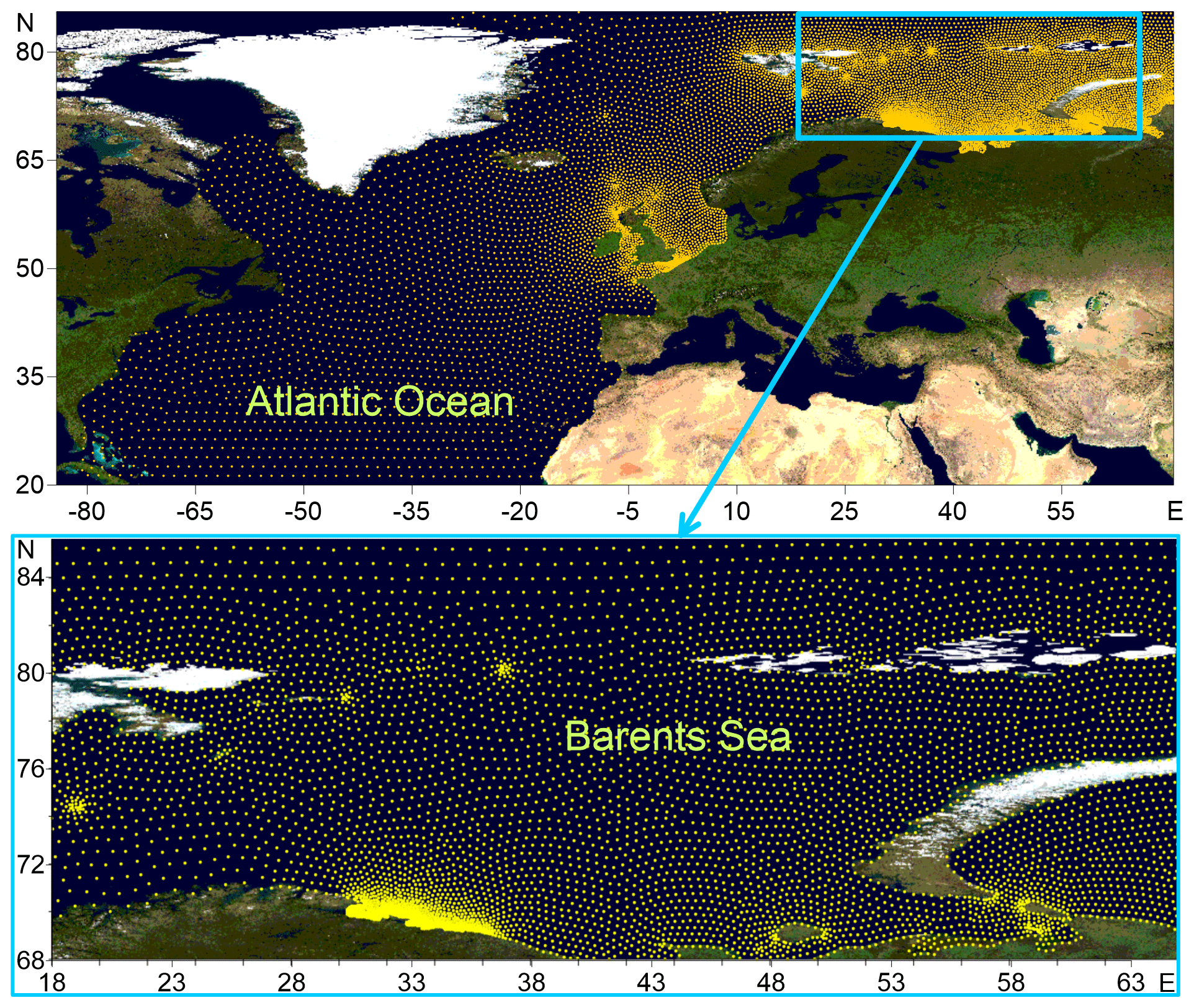
Figure 1 The computational unstructured grid for the Atlantic Ocean and the Barents Sea. The base map is the Blue Marble image obtained by connecting to the WMS Demo Server in the Golden Software Surfer program.

The general time step for the integration of the full wave equation was 15 min, the time step for the integration of functions of sources and sinks of wave energy was 60 s, and the time step for the spectral energy transfer and for satisfying the Courant–Friedrichs–Lewy condition was 450 s. This choice is dictated by the configuration of the computational grid: the maximum and minimum distances between the nodes and a large latitudinal extent.

The 10 m wind from the NCEP/CFSR reanalysis (Saha et al., 2010) for the period from 1979 to 2010 with a spatial resolution of $\sim \mathrm{0.3}{}^{\circ }$ was used as the forcing. Data from the NCEP/CFSv2 reanalysis (Saha et al., 2014) with a resolution of $\sim \mathrm{0.2}{}^{\circ }$ and with a time step of 1 h were used for the period from 2011 to 2017.

The wave model quality was assessed using the CryoSat satellite data for the 2010–2017 period (data collected from the IMOS satellite database; Ribal and Young, 2019). A comparison of the modeled and satellite-retrieved significant wave height (SWH) is shown in Fig. 2. The model accuracy metrics are 0.88 for the correlation coefficient (R), a bias of −0.04 m, a RMSE of 0.53 m, and a scatter index of 0.28. The results of the model quality assessments based on the satellite data are of the same quality as those found in previous studies (Stopa et al., 2016; Li et al., 2019).

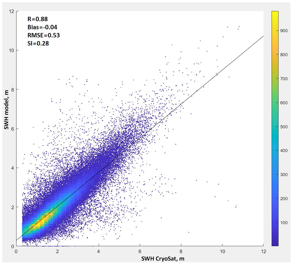
Figure 2 Scatter diagram of the significant wave height based on the model and satellite data.

In this paper, we used the output results of the wave model with a time step of 3 h from 1979 to 2017 for each node of the unstructured grid.

Based on the wave model results, a study of storm activity was carried out according to the POT (peak over threshold) method, which was used successfully in Myslenkov et al. (2019). For each year in the Barents Sea, the number of storm surges with different significant wave heights from 5 to 8 m was calculated. The event was counted as a storm with wave heights > 5 m if at least one node in the study area had wave heights exceeding the threshold of 5 m. The event continued until the wave heights in all nodes became less than the threshold. To eliminate possible errors, at least 9 h should pass between two storm events. Using the described procedure, a catalog of storm days was compiled when the significant wave heights of more than 5 m were observed. A total of 1964 d were identified for the 1979–2017 period.

2.2 COARE algorithm and the roughness parameter parameterization

Turbulent heat fluxes were calculated using the COARE algorithm (Fairall et al., 1996), based on the model of Liu, Katsaros and Businger (LKB) (Liu et al., 1979). Bulk formulae for the momentum and scalar fluxes have the following general form:

$$\begin{array}{}\text{(2)}& w^{\prime }{x}^{\prime }=c_x^{\mathrm{1}/\mathrm{2}}{c}_{\text{d}}^{\mathrm{1}/\mathrm{2}}S\mathrm{\Delta }X=C_{x}S\mathrm{\Delta }X,\end{array}$$

where w’ represents the fluctuations of vertical wind; x can be a horizontal wind component u, v, temperature or specific humidity; c_x represents transfer coefficients for x; c_d represents transfer coefficient for momentum; C_x represents the total transfer coefficient; ΔX is the difference of the mean x at a height equal to the roughness length and at a certain height (10 m) in the atmospheric surface layer (Fairall et al., 2003). S is the mean wind speed with gusts U_g:

$$S=\sqrt{U^{\mathrm{2}}+V^{\mathrm{2}}+U_{\text{g}}^{\mathrm{2}}}.$$

The default value of U_g is 0.5 m s⁻¹ in the COARE algorithm. Transfer coefficients depend on the roughness length and dimensionless universal functions. The form of universal functions in the COARE algorithm is set in accordance with Beljaars and Holtslag (1991) for stable stratification; the so-called Kansas functions (Kaimal et al., 1972) are used for unstable stratification; and functions from Fairall et al. (1996) and Grachev et al. (2000) are used for a very unstable stratification. For the roughness length, several parameterizations are available in the COARE algorithm. The parameterization of Charnock Charnock (1955) implies dependence of roughness on the friction velocity u_*:

$$\begin{array}{}\text{(3)}& z_{\mathrm{0}}={\displaystyle \frac{\mathit{\alpha }{u}_{*}^{\mathrm{2}}}{g}}+{\displaystyle \frac{\mathrm{0.11}a}{u_{*}}},\end{array}$$

where α is the Charnock parameter, g is gravity acceleration, and a is the kinematic viscosity coefficient (Andreas, 1989). Equation (3) is the modified Charnock formula (Smith, 1988), in which the second term on the right side describes the roughness over an aerodynamically smooth surface (i.e., in weak winds). The Charnock coefficient is set constant in strong and weak winds and is linearly dependent on the 10 m wind speed S in moderate winds:

$$\mathit{\alpha }=\left\{\begin{array}{ll}\mathrm{0.011},& S<\mathrm{10}\mathrm{m}{\mathrm{s}}^{-\mathrm{1}}\\ \mathrm{0.011}+\frac{\mathrm{0.007}(S-\mathrm{10})}{\mathrm{8}},& \mathrm{10}\mathrm{m}{\mathrm{s}}^{-\mathrm{1}}<S<\mathrm{18}\mathrm{m}{\mathrm{s}}^{-\mathrm{1}}\\ \mathrm{0.018},& S>\mathrm{18}\mathrm{m}{\mathrm{s}}^{-\mathrm{1}}.\end{array}\right.$$

In the parameterization of Taylor and Yelland (2001) (hereafter referred to as T1), the roughness length is related to the wave steepness ($H_{\text{s}}/L_{\text{p}}$):

$$\begin{array}{}\text{(4)}& z_{\mathrm{0}}=H_s{a}_{\mathrm{1}}{\left({\displaystyle \frac{H_{\text{s}}}{L_{\text{p}}}}\right)}^{b_{\mathrm{1}}}+{\displaystyle \frac{\mathrm{0.11}a}{u_{*}}},a_{\mathrm{1}}=\mathrm{1200},b_{\mathrm{1}}=\mathrm{4.5},\end{array}$$

where H_s is the significant wave height, and L_p is the spectral peak wavelength.

The parameterization of Oost et al. (2002) (hereafter referred to as O2) implies the dependence of the roughness length on the spectral peak wavelength L_p and the inverse wave age ($u_{*}/c_{\text{p}}$):

$$\begin{array}{}\text{(5)}& z_{\mathrm{0}}=L_{\text{p}}{a}_{\mathrm{2}}{\left({\displaystyle \frac{u_{*}}{c_{\text{p}}}}\right)}^{b_{\mathrm{2}}}+{\displaystyle \frac{\mathrm{0.11}a}{u_{*}}},a_{\mathrm{2}}=\mathrm{50}/\mathrm{2}\mathit{\pi },b_{\mathrm{2}}=\mathrm{4.5}.\end{array}$$

Here, c_p is the phase wave speed associated with spectral peak, which is expressed through the wave length as $c_{\text{p}}=\sqrt{L_{\text{p}}g/\mathrm{2}\mathit{\pi }}$.

Finally, we included the parametrization of Drennan et al. (2003) (hereafter referred to as D3) in the COARE algorithm. The D3 parameterization consists in the dependence of the roughness length on the wave height and the inverse wave age:

$$\begin{array}{}\text{(6)}& z_{\mathrm{0}}=H_{\text{s}}{a}_{\mathrm{3}}{\left({\displaystyle \frac{u_{*}}{c_{\text{p}}}}\right)}^{b_{\mathrm{3}}}+{\displaystyle \frac{\mathrm{0.11}a}{u_{*}}},a_{\mathrm{3}}=\mathrm{3.35},b_{\mathrm{3}}=\mathrm{3.4}.\end{array}$$

Thus, the main components of the algorithm are the Eq. (2), the formulae for calculating transfer coefficients based on the Monin–Obukhov similarity theory, and Eqs. (3)–(6) for the roughness length. Thus, in general, the COARE algorithm is similar to corresponding algorithms in most atmospheric models.

Using the COARE algorithm, we calculated turbulent sensible and latent heat fluxes in the Barents Sea from 1979 to 2017. Mean fluxes were calculated for a long-term period and for periods of cold-air outbreaks and storm wave events. As the scatter index of our modeled significant wave heights is 0.28 (or 28 %), this value can probably lead to mean errors of ∼4 %–5 % in the calculated heat flux values when the wave heights is ∼5 m.

2.3 Input data for the COARE algorithm

Input data for the COARE algorithm are wind vector, air temperature, sea surface temperature (SST), air humidity, incoming shortwave and longwave radiation, precipitation intensity, and sea wave height and period. The NCEP/CFSR and CFSv2 (Saha et al., 2010, 2014) reanalyses with a temporal resolution of 6 h for the total 1979–2017 period were used as atmospheric data input for the COARE algorithm. CFSv2 reanalysis data for the 2011–2017 period (with a slightly better spatial resolution than CFSR) were interpolated from a $\sim \mathrm{0.2}{}^{\circ }$ grid to a $\sim \mathrm{0.3}{}^{\circ }$ grid to match the CFSR resolution. The wind speed was used at 10 m height, and air temperature and humidity were used at 2 m height. Reanalysis data are also available at isobaric levels, the lower of which is 1000 hPa. However, we preferred to take diagnostic variables at heights of 2 and 10 m for several reasons. Firstly, the height of the isobaric levels varies greatly. Secondly, data at vertical levels are available on a much coarser grid (0.5^∘). For instance, Arthun and Schrum (2010) also used diagnostic variables at standard levels from the NCEP/NCAR reanalysis to calculate turbulent fluxes in the ocean model. The surface pressure and the inversion height (boundary layer height), which are usually set constant in the COARE algorithm, were obtained from the CFSR reanalysis (at each time and at each grid point).

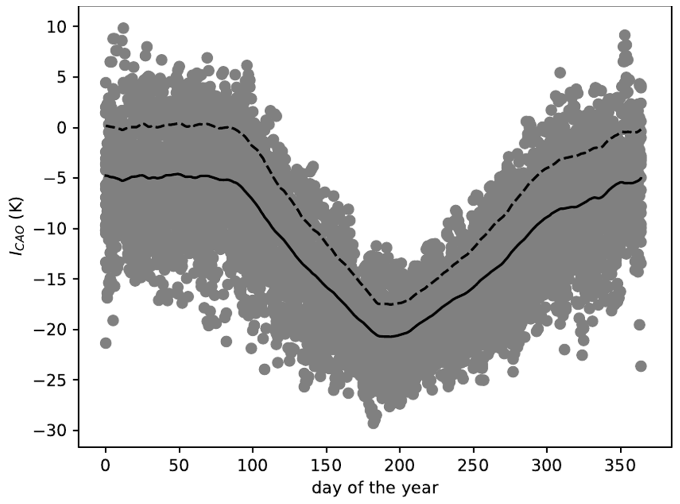
Figure 3 Cold-air outbreak index (I_CAO) for the 1997–2017 period. The solid curve represents the 30 d running multiyear mean values ($\stackrel{\mathrm{‾}}{I_{\text{CAO}}}$). Extreme CAOs correspond to points above the dashed curve, which is the sum of $\stackrel{\mathrm{‾}}{I_{\text{CAO}}}+{\mathit{\sigma }}_I$, where the latter is the 30 d running multiyear standard deviation of I_CAO.

2.4 Ship observations

We used ship observations in the Barents Sea from the NABOS expeditions in 2005, 2007, 2013 and 2015 to verify turbulent heat fluxes calculated using the COARE algorithm. All expeditions took place in the period from August to October. Shipborne fluxes were calculated using the eddy-covariance method (the left side of Eq. 2) based on high-frequency measurements of temperature and the three wind components using Gill and Metek sonic anemometers (Ivanov et al., 2019). The averaging period for the covariance calculations was 10 min. For all wind measurements, a correction was made for the movement of the ship. A detailed description of the location of the instruments and the methods for filtering data and calculating fluxes is available at https://uaf-iarc.org/nabos-cruises/ (last access: 26 June 2020). For verification, the calculated values of heat fluxes were bilinearly interpolated (using four surrounding points) from the CFSR reanalysis grid to the ship coordinates.

2.5 Identification of CAOs

The so-called “CAO index” is frequently used for CAO identification. It was first defined (Kolstad and Bracegirdle, 2008; Kolstad et al., 2009) as the potential temperature difference between the ocean surface and the 700 hPa height normalized by the pressure difference at the same heights. The original authors used the value of the 90th percentile of the CAO index to estimate the strength and frequency of occurrence of CAOs. Other investigators (e.g., Fletcher et al., 2016) used the non-normalized potential temperature difference between the surface and the 800 hPa height as metrics to study the frequency and strength of CAOs, and they evaluated the frequency of occurrence of the positive values of the CAO index as well as the value of the 95th percentile of the CAO index during the winter months.

Here, we define the CAO index I_CAO as the daily potential temperature difference between the ocean surface and the 700 hPa height. For each day, I_CAO was averaged over the ice-free part of the Barents Sea. Figure 3 shows the obtained I_CAO values for the 1979–2017 period. The solid curve in Fig. 3 consists of the multiyear-averaged values ($\stackrel{\mathrm{‾}}{I_{\text{CAO}}}$) obtained by (1) averaging I_CAO over a 30 d period centered on the given day and (2) averaging the obtained values over the years. Similarly, the standard deviation (σ_I) of I_CAO was obtained.

The dashed curve in Fig. 3 represents the threshold value $\stackrel{\mathrm{‾}}{I_{\text{CAO}}}+{\mathit{\sigma }}_I$ that we use as a criteria for CAO identification, namely

$$\begin{array}{}\text{(7)}& I_{\text{CAO}}>\stackrel{\mathrm{‾}}{I_{\text{CAO}}}+{\mathit{\sigma }}_I.\end{array}$$

According to the criteria in Eq. (7), we identify CAOs as cases where I_CAO values are above the dashed curve in Fig. 3. A similar procedure has been used in other studies (e.g., Wheeler et al., 2011) to identify continental CAOs where authors simply used the air temperature at 2 m height instead of I_CAO.

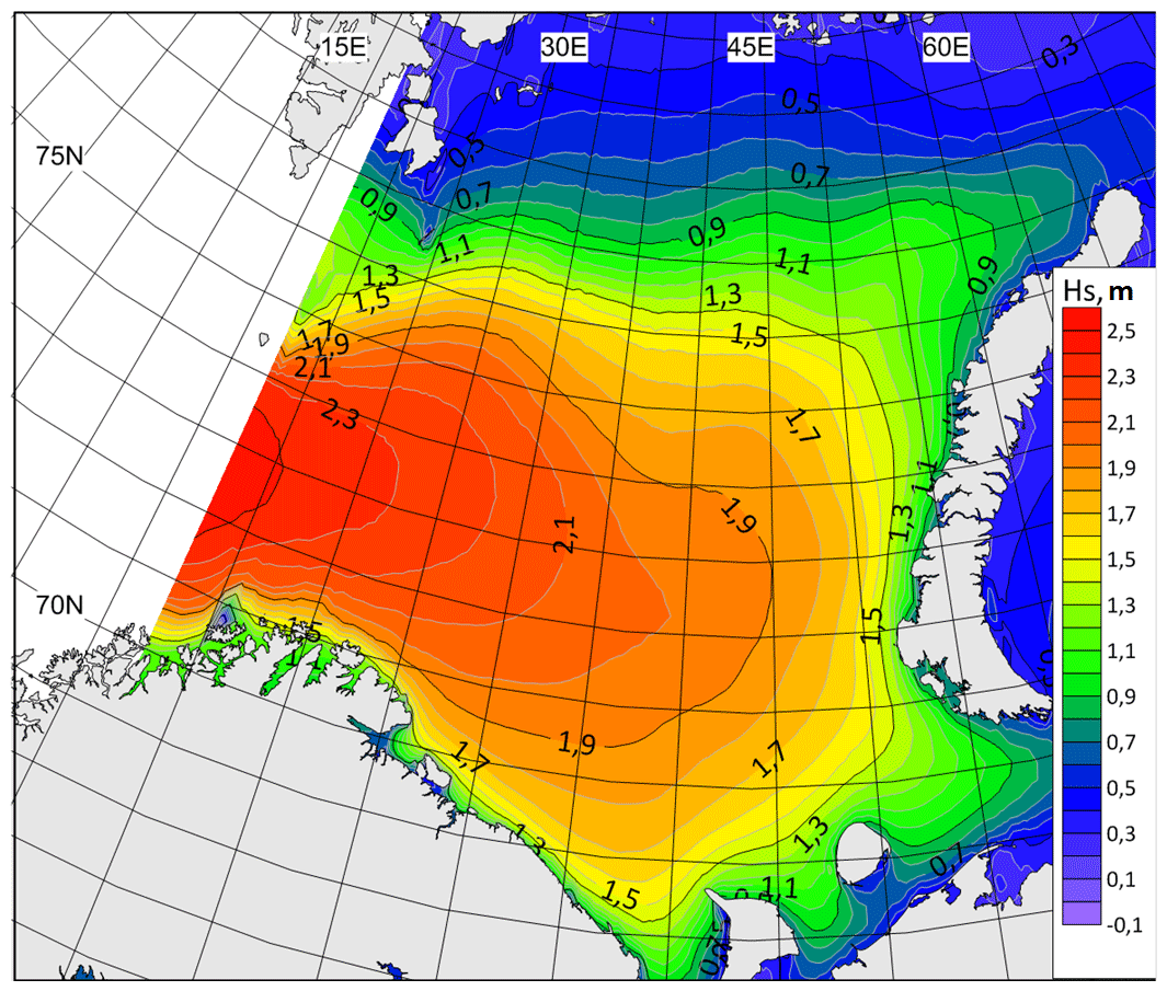
Figure 4 Long-term average significant wave height in the Barents Sea based on the WWIII simulation results for the 1979–2017 period.

Figure 3 shows that the largest values of I_CAO are observed in a period from the second half of December until the end of March, when the coldest air advection occurs over the Barents Sea. It is interesting to note that in winter the criteria in Eq. (7) is almost identical to I_CAO>0. The latter serves as a measure of the dry hydrostatic stability of the layer between the ocean surface and the 700 hPa surface. Thus, positive values of I_CAO indicate conditions favorable for mixed-layer development to heights over 700 hPa. During strong background advection, the mixed layer can only reach such heights at a significant distance from the ice edge (Chechin and Lüpkes, 2017).

3 Results

3.1 Wave climate and storm activity

First, we consider the main features of wave conditions and wave climate in the Barents Sea, which directly affect the processes of heat exchange in the ocean–atmosphere system. In Fig. 4, the average significant wave heights for the entire simulation period from 1979 to 2017 are shown. The highest average wave heights are found in the western part of the sea. Here, we can expect the greatest influence of sea waves on heat fluxes. In the north, due to the presence of ice, the average wave heights do not exceed 1 m.

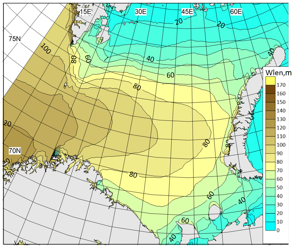
Figure 5 Long-term average spectral peak wavelength in the Barents Sea based on the WWIII simulation results for the 1979–2017 period.

Also, an equally important parameter is the wavelength, which is used in parameterizations O2 and D3. In Fig. 5, the mean long-term spectral peak wavelength is shown. The wavelengths from 80 to 100 m are observed in the central and western parts of the Barents Sea. The results on the average wave height and wavelength in general are consistent with similar works by other authors (Semedo et al., 2011; Stopa et al., 2016). Estimates of storm activity based on such long-term analysis are relatively rare, and a detailed analysis is outside the scope of this paper.

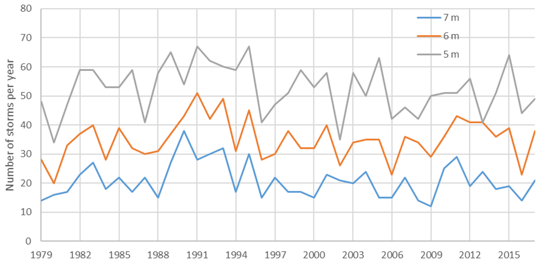
Figure 6 The number of storms with a significant wave height of more than 5, 6 and 7 m according to the WWIII simulation results for the 1979–2017 period.

The Barents Sea is characterized by a high frequency of storm wave events, which provide a long swell in the extinction stage (i.e., “old seas”) and limit the applicability of the Charnock formula. As shown in Myslenkov et al. (2018a), the number of storms per year in the Barents Sea can differ significantly. Figure 6 shows the number of storms calculated according to the wave model results with wave heights of more than 5 m and more than 7 m (identified as described in Sect. 2.1). During the period from 1979 to 2017, several maxima of storm activity were observed (e.g., in 1989–1991 and in 2011). Especially for these periods, the calculated heat fluxes are expected to be sensitive to the parameterizations of the roughness length used (see Sect. 3.5).

Figure 7 The number of days with CAOs over the Barents Sea selected using Eq. (7) for each cold season in 1979–2018.

3.2 CAOs' frequency of occurrence

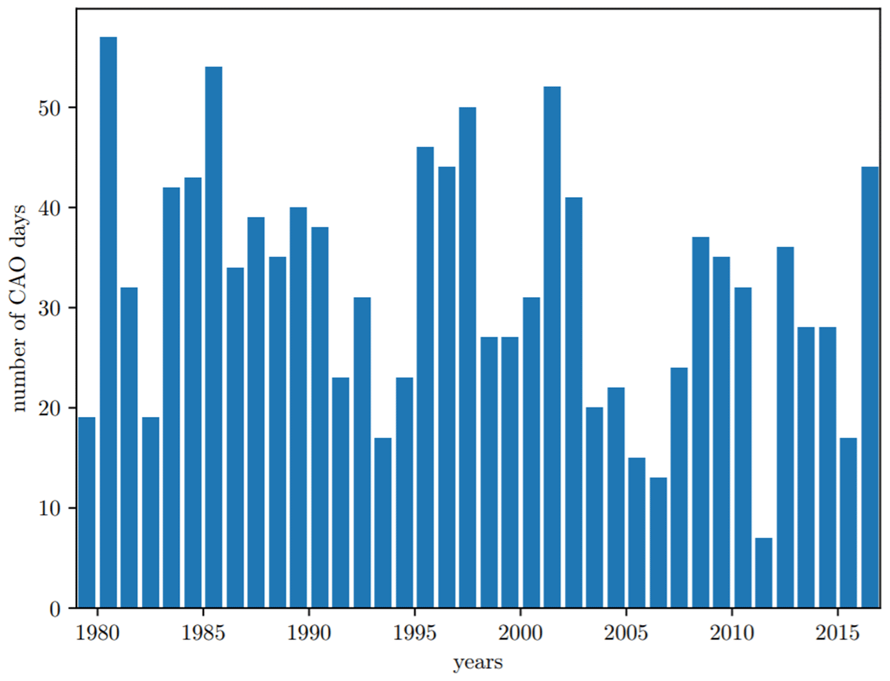
Figure 7 shows the time series of the number of days with extreme CAOs selected using Eq. (7) for each cold period (November–April) from 1979 to 2018. On average, CAOs are observed on 16.4 % of days. However, the interannual variability of the frequency of occurrence of CAOs is large. Namely, the interannual standard deviation of the number of CAO days amounts to 12 d. Thus, the number of CAO days per cold season varies from 6 in 2011–2012 to 56 in 1980–1981.

The frequency of occurrence of CAOs over the Barents Sea is governed by the variability of the large-scale patterns of atmospheric circulation. To the largest extent, the frequency of CAOs is correlated with the so-called “Barents Oscillation” (Skeie, 2000; Wu et al., 2006; Kolstad et al., 2009). The latter is the mode of variability of the sea level pressure field represented by a dipole with high pressure over Greenland and Iceland and low pressure over the northern part of the European section of Russia. Such a pressure field promotes intense cold-air advection over the Barents Sea from the north. Moreover, there is a negative correlation between the North Atlantic Oscillation index and CAOs' frequency of occurrence (Kolstad et al., 2009). Such a correlation is particularly strong for easterly CAOs, which is obviously associated with the reduced strength of the westerlies.

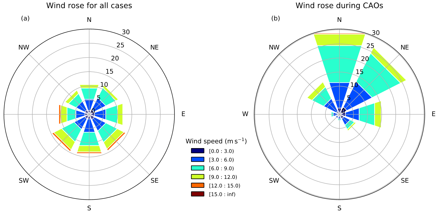
Figure 8 Frequency of occurrence of daily 10 m wind speed and direction, averaged over the ice-free part of the Barents Sea for the November–April period from 1979 to 2018 for all cases (a) and for cold-air outbreaks (b).

A slight negative trend of the CAO days is seen in Fig. 7. To a large extent, it can be explained by an increase in the mean CAO index values over the Barents Sea. Such an increase can be associated either with a higher air temperature over the Arctic in winter, i.e., CAOs become less severe, or with a decrease in the frequency of synoptic patterns favorable for CAOs (Papritz and Grams, 2018). A negative trend of the CAO index values over the Barents and Kara seas was also obtained by Narizhnaya et al. (2020) based on the ERA-Interim data for the 1979–2018 period. They found an increase in the number of weak and moderate CAOs and a decrease in the number of strong CAOs.

The frequency of CAOs with easterly wind over the Barents Sea is significant and represents up to 16 % of all CAOs (Fig. 8b). During CAOs, the highest frequency of occurrence is observed for northerly (30 %) and northeasterly (27 %) winds. The wind rose in CAOs differs from the wind rose in all cases during the cold season (Fig. 8a). In particular, the prevailing wind direction over the Barents Sea in winter is from the south. Moreover, the winds with southerly and westerly components are the strongest.

The CAOs' role in the heat exchange between the Barents Sea and the atmosphere is demonstrated by Fig. 9. The figure shows the turbulent fluxes of sensible and latent heat, H and LE, respectively, the net longwave radiative flux LW_net, and the total heat flux $F_{\text{total}}=H+LE+{\text{LW}}_{\text{net}}$ averaged over the November–April period over the ice-free part of the Barents Sea as functions of the number of CAO days during the same period. Clearly, there is a strong dependency of the Barents Sea heat loss on the number of CAO days. The highest correlation coefficients are obtained for LW_net, F_total and H and amount to 0.86, 0.85 and 0.84, respectively. A smaller correlation coefficient of 0.78 is obtained for LE. Also, the coefficients of linear regression shown in Fig. 9 demonstrate that F_total has the strongest dependency on the number of CAO days. From all terms of the surface heat balance, the sensible heat flux H is most sensitive to the number of CAO days. All of the three components of the surface heat balance that were considered (H, LE and LW_net) manifest heat loss from the sea surface to the atmosphere and are of a comparable magnitude of about 70 W m⁻² on average.

We stress that the values of fluxes shown in Fig. 9 are averaged over the ice-free part of the Barents Sea. It is important to keep in mind that there is a large interannual variability with respect to the area of sea ice cover in the Barents Sea. This is another important factor, along with the number of CAO days, influencing the heat loss.

One might also expect that the ice edge retreat further north leads to a larger fetch over which the cold air mass is advected. This would result in a higher air temperature over the Barents Sea which could locally decrease the surface heat flux (Pope et al., 2020). However, this would lead to an increase in the total heat loss at the surface of the Barents Sea which is proportional to the open-water area. As the sensible heat flux maximum during CAOs is located near the ice edge, the maximal heat loss location would also shift further north. This might have implications for the so-called “Atlantification” in the northeastern part of the Barents Sea (e.g., Barton et al., 2018).

3.3 Verification of the COARE algorithm by ship observations

Figure 10 shows the comparison of sensible and latent heat fluxes from shipborne observations that were calculated using different roughness parameterizations, namely Charnock (1955), C55; Taylor and Yelland (2001), T1; Oost et al. (2002), O2; and Drennan et al. (2003), D3. Figure 10a–c present calculations made on the basis of reanalysis, interpolated to the cruise track, whereas Fig. 10d–f present calculations from shipborne observations of meteorological parameters and radiative fluxes (available only in 2013–2015).

The correlation coefficient between the observed and the calculated fluxes from reanalysis data (Fig. 10a, b) is 0.7 for the sensible heat flux and 0.8 for the latent heat flux. However, the mean absolute error (MAE) is rather large – about 20 W m⁻². The error magnitude increases with the increase in the heat flux magnitude. The error may be connected to both the COARE algorithm itself and to the input data (i.e., related to the quality of meteorological parameters in the reanalysis). For example, a strong overestimation of heat fluxes on 11–12 October 2007 is associated with the overestimation of wind speed (by 6–8 m s⁻¹) compared with observations.

In order to estimate the accuracy of the COARE algorithm itself and to exclude the reanalysis error, we additionally performed calculations on the basis of shipborne meteorological observations (Fig. 10d–f). In these calculations we set precipitation intensity at zero and boundary layer height at 600 m, as these parameters were not observed. The correlation coefficient between the observed and the calculated fluxes from the observational data is 0.98–0.99; MAE is reduced to ∼4 W m⁻² for sensible heat flux and to ∼8 W m⁻² for latent heat flux. This error is within the accuracy of the eddy-covariance method. The accuracy of this method in the case of ship measurements can be significantly reduced due to the influence of air flow distortion by the ship. Therefore, we can conclude that the calculated fluxes are in good agreement with the observations.

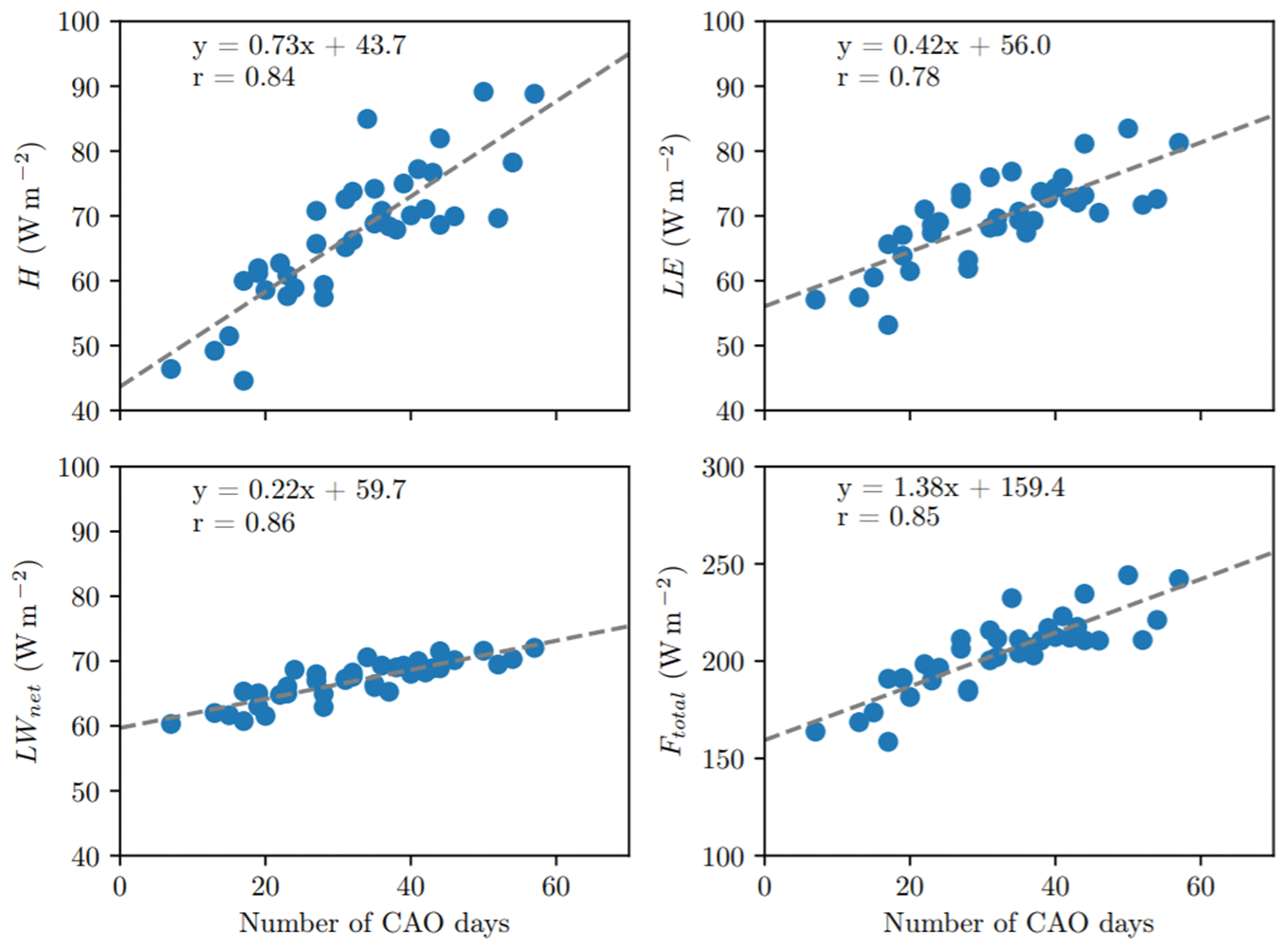
Figure 9 Turbulent fluxes of sensible and latent heat (H and LE, respectively), net longwave radiative flux (LW_net) and the total heat flux (F_total) averaged over the cold season (November–April) and over the ice-free part of the Barents Sea as a function of number of CAO days during the same period for 1979–2018. The dashed line shows the linear regression line, whose equation is given in each plot, as well as the correlation coefficient (r).

Heat fluxes calculated with different roughness parameterizations are almost identical (Fig. 10); the average difference between them is 1 W m⁻². This difference is highest in October 2007 and September 2015 (up to 11 % of the heat fluxes magnitudes) when the inverse wave age (Fig. 10c, f) is greater than 0.05, which is a threshold for young sea. The calculated roughness length (Fig. 10c, f) differs by up to 7 times for those cases. However, most cases are characterized by a developed sea situation ($u_{*}/c_{\text{p}}<\mathrm{0.05}$), when all parameterizations should behave well (Drennan et al., 2005). This must also be the reason for small differences in roughness length and heat fluxes. The small difference between parameterizations makes it impossible to unambiguously define the parametrization that fits the observations better.

3.4 Long-term mean turbulent heat fluxes

Here, we consider the mean long-term values of heat fluxes calculated from the CFSR reanalysis data using COARE algorithm and various roughness parameterizations. The mean long-term (1979–2017) sensible and latent heat flux obtained in the C55 experiment and the differences between experiments are shown in Figs. 11 and 12. The main conclusion of these results is the presence of positive difference for the T1 and O2 experiments and a negative difference for the D3 experiment. The long-term values of the difference are small: 1–2 W m⁻² for T1 and 0.5–1 W m⁻² for O2.

Tables 1 and 2 show the average statistics: the difference in heat fluxes with and without explicitly accounting for sea wave parameters. Over the entire Barents Sea, the full range of differences in the fluxes is small, from −3 to +2 W m⁻², which is only 1 %–3 % of the mean absolute value. The greatest mean difference for sensible heat flux was observed for T1, and the greatest mean difference for latent heat flux was observed for the O2 parametrization.

The flux difference can exceed 30–50 W m⁻² (in 0.1 % of cases or the 99.9th percentile) and in some extreme cases reach 100–250 W m⁻². The highest maxima of the flux difference are obtained for the O2 experiment.

Table 1 Statistical characteristics of the difference in the sensible heat flux calculated with and without explicitly accounting for sea wave parameters: mean difference, relative mean (ratio of the mean difference to the mean value of the flux), mean absolute difference, 95th and 99.9th percentile, and the maximum difference for the Barents Sea

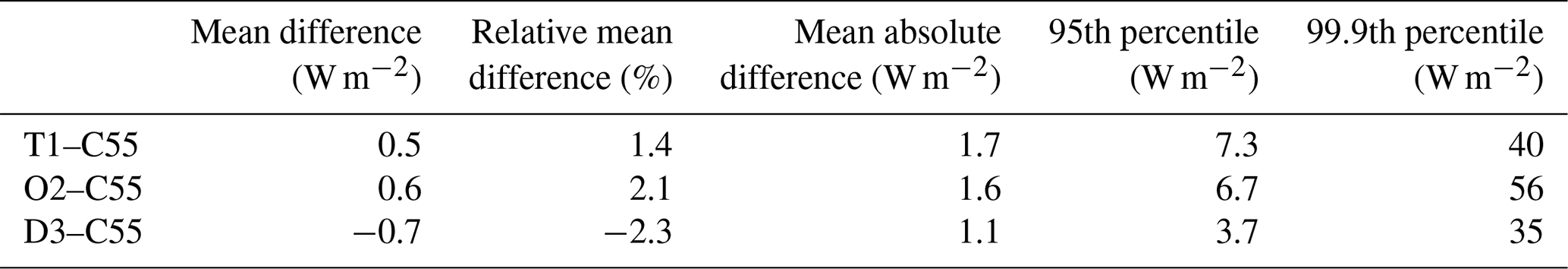
Table 2 Statistical characteristics of the difference in the latent heat flux calculated with and without explicitly accounting for sea waves: mean, relative mean (ratio of the mean difference to the mean value of the flux), mean absolute difference, 95th and 99.9th percentile, and the maximum difference for the Barents Sea

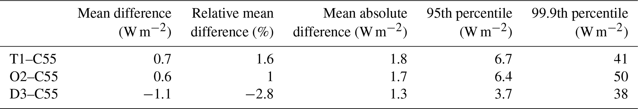
Figure 10 Sensible (a, d) and latent (b, e) heat fluxes and roughness length (c, f) according to NABOS observations (black solid line) and calculated using various roughness parameterizations (solid colored lines). Calculations are made with reanalysis (a–c) and observation data (d–f) (where observations of wind speed, temperature and radiative fluxes are available). Also, significant wave height H_s from WWIII simulations (a–d), wind speed from reanalysis (b) and observations, (e) and inverse wave age $u_{*}/c_{\text{p}}$ (c, f) are shown.

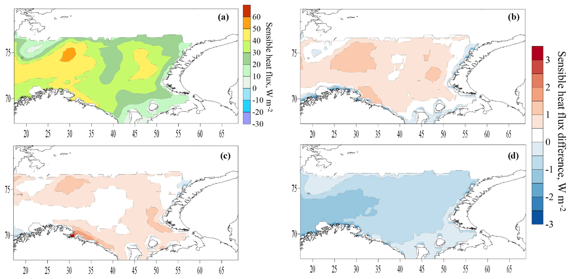
Figure 11 Mean sensible heat flux in experiment C55 (a) and the difference in the sensible heat fluxes between experiments T1–C55 (b), O2–C55 (c) and D3–C55 (d). All grid nodes where sea ice was in more than half of the cases are filtered out.

The greatest differences between the experiments are found in those areas where the highest values of the heat fluxes are observed. This can be explained by the power law dependence of the roughness length on the friction velocity/wave height. Moreover, in the O2 parameterization, the proportionality coefficient is larger (a₂=4.5) than in the D3 parameterization (a₃=3.4), which is reflected in the flux differences.

A more detailed spatial analysis of the 99.9th percentile of sensible heat flux difference is shown in Fig. 13. The extreme values of the flux difference taking the O2–C55 difference as an example showed that some of the extrema are associated with coastal areas, mainly off the western coast of Novaya Zemlya during bora. Other extremes were associated with deep cyclones in different parts of the sea, with different distances from the coast. Some extremes are associated with storm waves or are observed immediately after storms, during cold-air outbreaks at the rear of cyclones. Therefore, the characteristics of heat fluxes during storm waves and cold-air outbreaks will be considered separately in the following sections.

3.5 Turbulent heat fluxes during storm wave events

Here, we consider turbulent heat fluxes during the storms identified in Sect. 3.1 (a total of 1964 d with storms for the 1979–2017 period). The spatial distribution of heat fluxes during storms (Figs. 14, 15) resembles the average distribution (Figs. 11, 12), but the absolute values increase by almost a factor of 2. The average sensible heat flux has several maxima – in the northwest of the sea, near the coast of the Kola Peninsula and a less pronounced local maximum off the southern island of Novaya Zemlya. The flux difference between the experiments is also distributed the same way on average and increases in absolute value (except for experiment D3). The average flux difference between experiments reaches 4–5 W m⁻² for T1–C55, 8 W m⁻² for O2–C55 and 3–4 W m⁻² for D3–C55. On average, the relative difference in heat fluxes is 3 % for T1–C55 and 3 %–5 % for O2–C55. The correlation coefficient between the magnitude of the flux and the magnitude of the flux difference is 0.9. For the D3 experiment, the flux difference gradually increases from east to west, and some special structures associated precisely with storms do not appear. The detected maxima of flux difference in the western part of the sea generally correspond to the maxima of the average wave height (Fig. 4).

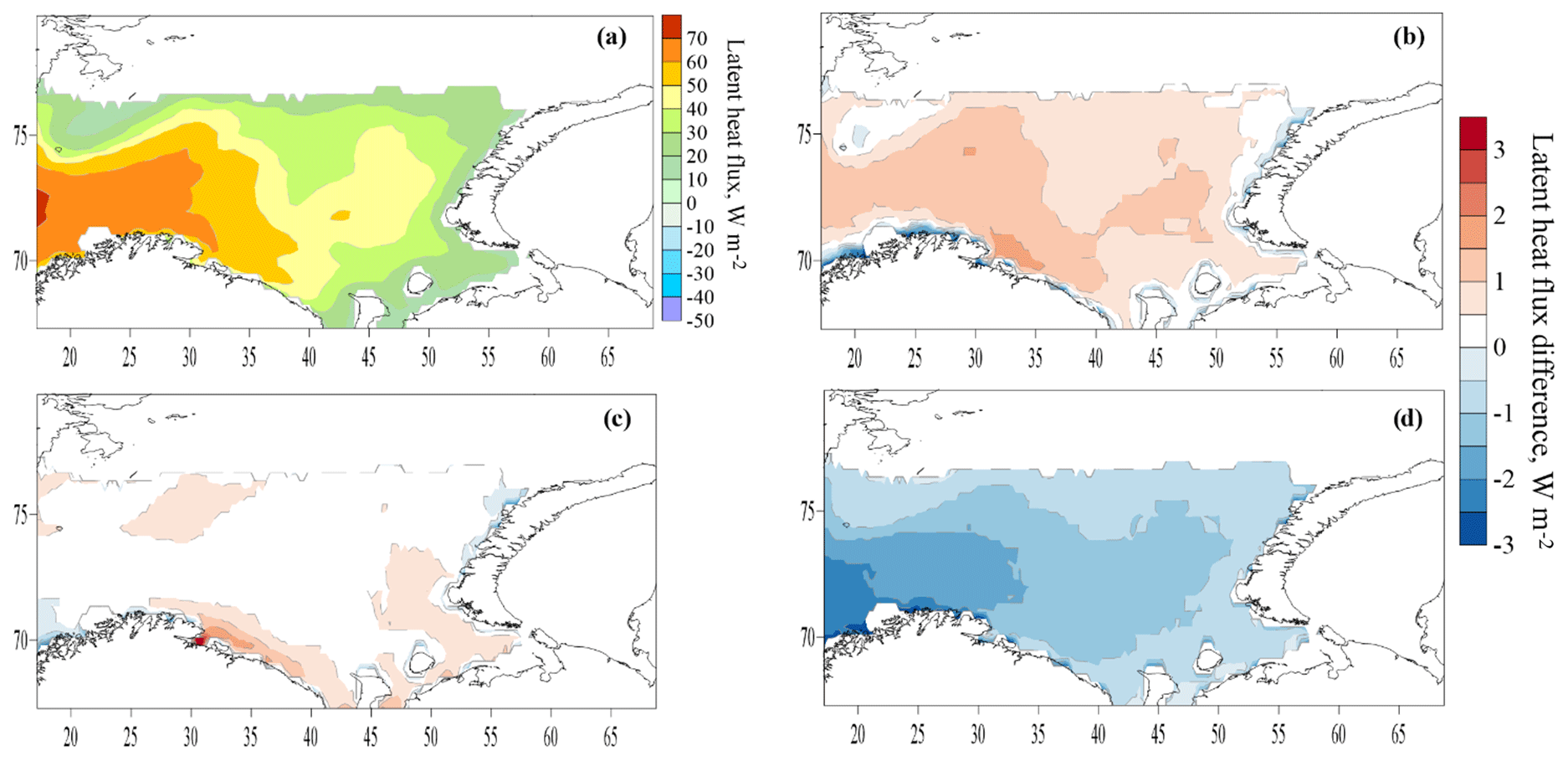
Figure 12 Mean latent heat flux in experiment C55 (a) and the difference in the latent heat fluxes between experiments T1–C55 (b), O2–C55 (c) and D3–C55 (d). All grid nodes where sea ice was in more than half of the cases are filtered out.

It can be concluded that the mean pattern of heat fluxes in the Barents Sea is largely due to storms.

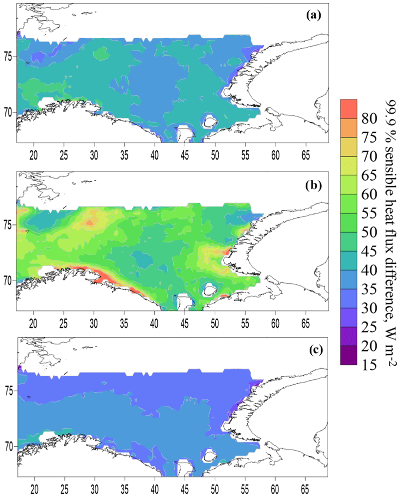
Figure 13 The 99.9th percentile of the sensible heat flux difference between experiments T1–C55 (a), O2–C55 (b) and D3–C55 (c).

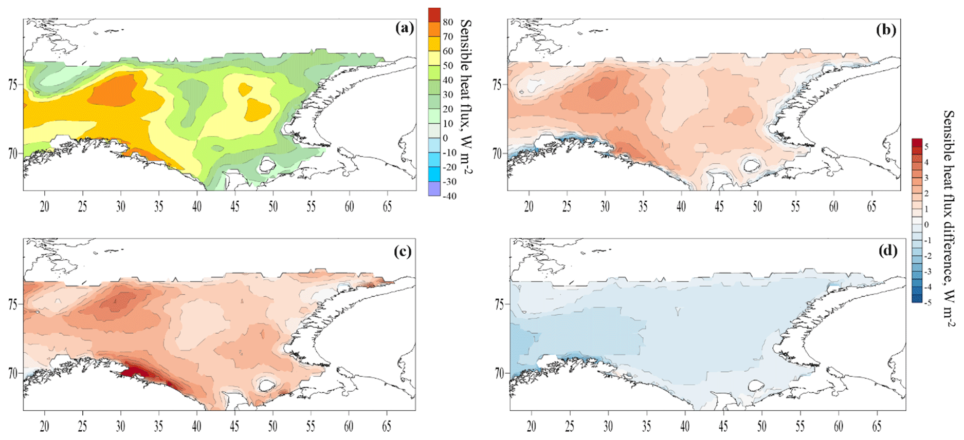
Figure 14 Mean sensible heat flux in experiment C55 (a) and the flux difference in experiments T1–C55 (b), O2–C55 (c) and D3–C55 (d) during storms.

3.6 Turbulent heat fluxes during cold-air outbreaks

Here, we consider turbulent heat fluxes during cold-air outbreaks identified in Sect. 3.2 (2326 d with cold-air outbreaks for the 1979–2017 period). The average values of the sensible heat flux increase, especially in the northwestern part (2 times compared with the average), during cold-air outbreaks (Fig. 16a). The spatial distribution of the latent heat flux is almost the same as the average one, but the flux magnitude increases by 1.5 times (Fig. 17a).

Experiments T1 and O2 increase the magnitude of the sensible and latent heat fluxes everywhere compared with C55 during cold-air outbreaks (Figs. 16, 17). Explicitly accounting for the storm wave events leads to an increase in heat fluxes mainly in the northwest of the sea and near the ice edge. However, the differences between the experiments are still small – on average less than 4 W m⁻² for the sensible heat flux and less than 2.5 W m⁻² for the latent heat flux, i.e., less than 3 %–4 % of flux magnitudes (Figs. 16, 17). At the same time, the extreme values of the flux difference during cold-air outbreaks, as for storm waves, are several times smaller than when considering long-term means.

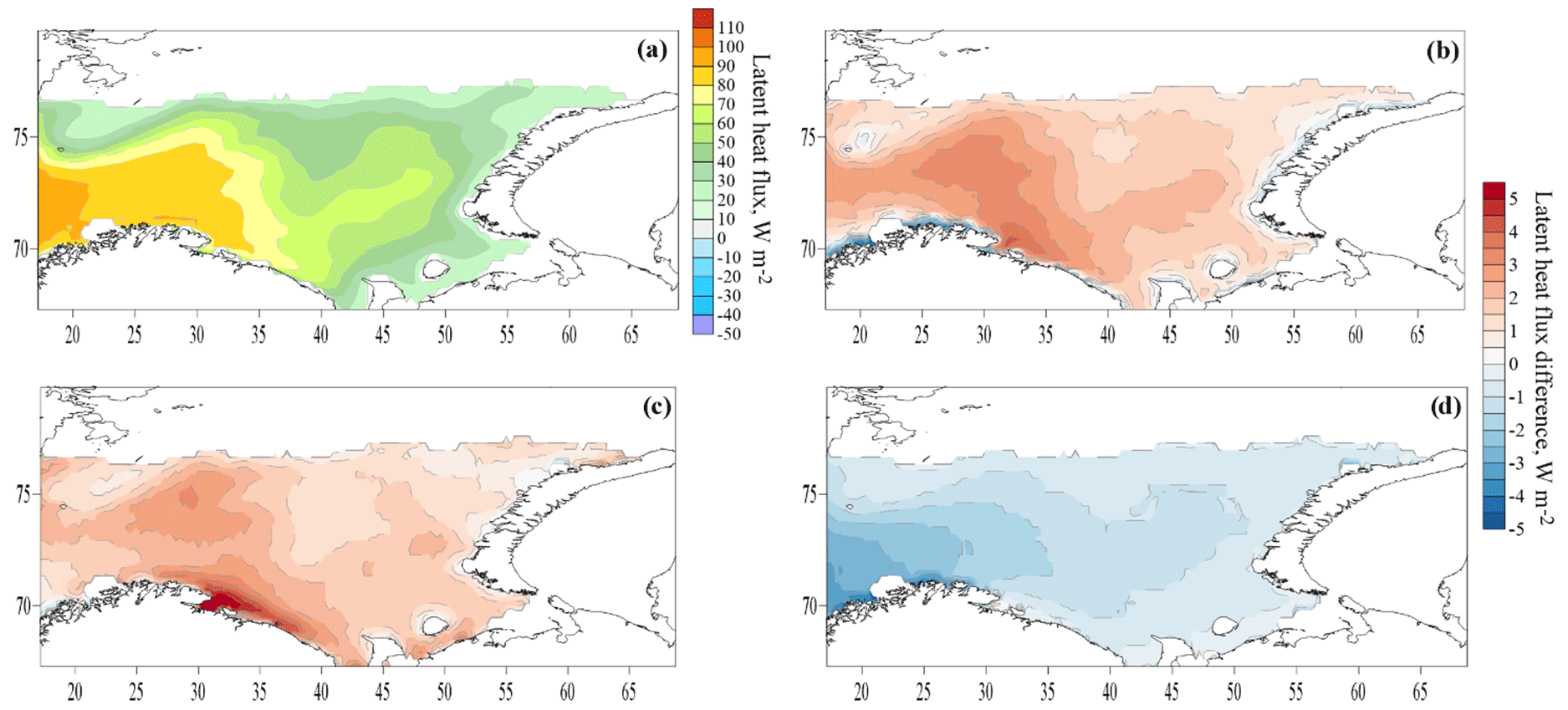
Figure 15 Mean latent heat flux in experiment C55 (a) and the flux difference in experiments T1–C55 (b), O2–C55 (c) and D3–C55 (d) during storms.

The average values of the flux difference during cold-air outbreaks are smaller than during storms, but the extreme values during cold-air outbreaks and during storms are close.

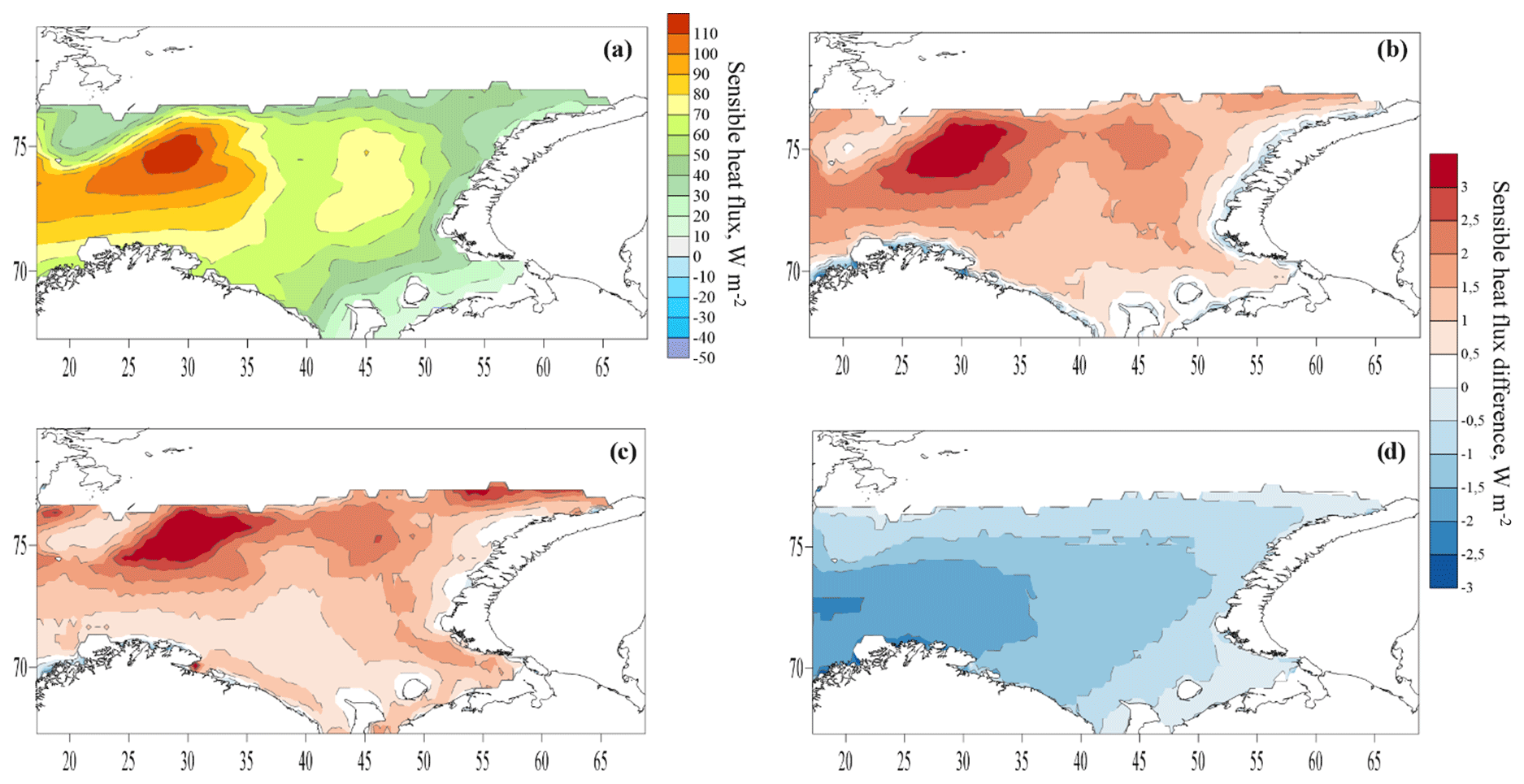
Figure 16 Mean sensible heat flux in experiment C55 (a) and the flux difference in experiments T1–C55 (b), O2–C55 (c) and D3–C55 (d) during cold-air outbreaks.

Figure 17 Mean latent heat flux in experiment C55 (a) and the flux difference in experiments T1–C55 (b), O2–C55(c) and D3–C55 (d) during cold-air outbreaks.

3.7 Turbulent heat fluxes during the simultaneously observed storm wave events and cold-air outbreaks

Finally, we consider cases when cold-air outbreaks and storm wave events were simultaneously observed (a total of 292 d for the 1979–2017 period) (Figs. 18, 19). The magnitude of the heat fluxes and the difference between the experiments in these cases are the largest in comparison with other situations. The sensible heat flux in experiment C55 reaches 170 W m⁻² (in the northwest of the sea), and the latent heat flux is 140 W m⁻² (in the west). The average T1–C55 difference reaches 6 W m⁻² for sensible heat flux and 4.5 W m⁻² for latent heat flux. The average O2–C55 difference reaches 10 W m⁻² for sensible heat flux and 7 W m⁻² for latent heat flux. The average D3–C55 difference reaches 3 W m⁻² in the west of the sea.

The extreme values of the difference, which can reach 700 W m⁻², are also greatest in the case of simultaneously observed storms and cold-air outbreaks. Figure 20 shows a case where the difference in sensible heat fluxes exceeded 100 W m⁻² between the C55 and T1 parameterizations and 400 W m⁻² between the C55 and O2 parameterizations. The greatest difference is noted for the eastern local maximum of the heat flux. There, the wind was from the southeast (on the front side of the cyclone) and reached 15–20 m s⁻¹; however, wave height and especially wave length were rather low due to a short fetch. The storm cyclone was moving very fast over the Barents Sea, which resulted in fast changes in wind direction and velocity on the eastern side of the sea. Thus, it was a very young sea state that resulted in such a difference between parameterizations. An analysis of other cases in which extreme values of the flux difference were observed also showed the presence of two local maxima (western and eastern) of heat fluxes. The same maxima also appear in the long-term mean pattern of heat fluxes (Figs. 16, 17) and are associated with the cyclone structure and sea ice edge configuration: strong southeasterly winds in front of the cyclone and northerly winds at the rear of cyclones both produce young waves on short fetches that contribute greatly to augmented roughness and heat fluxes.

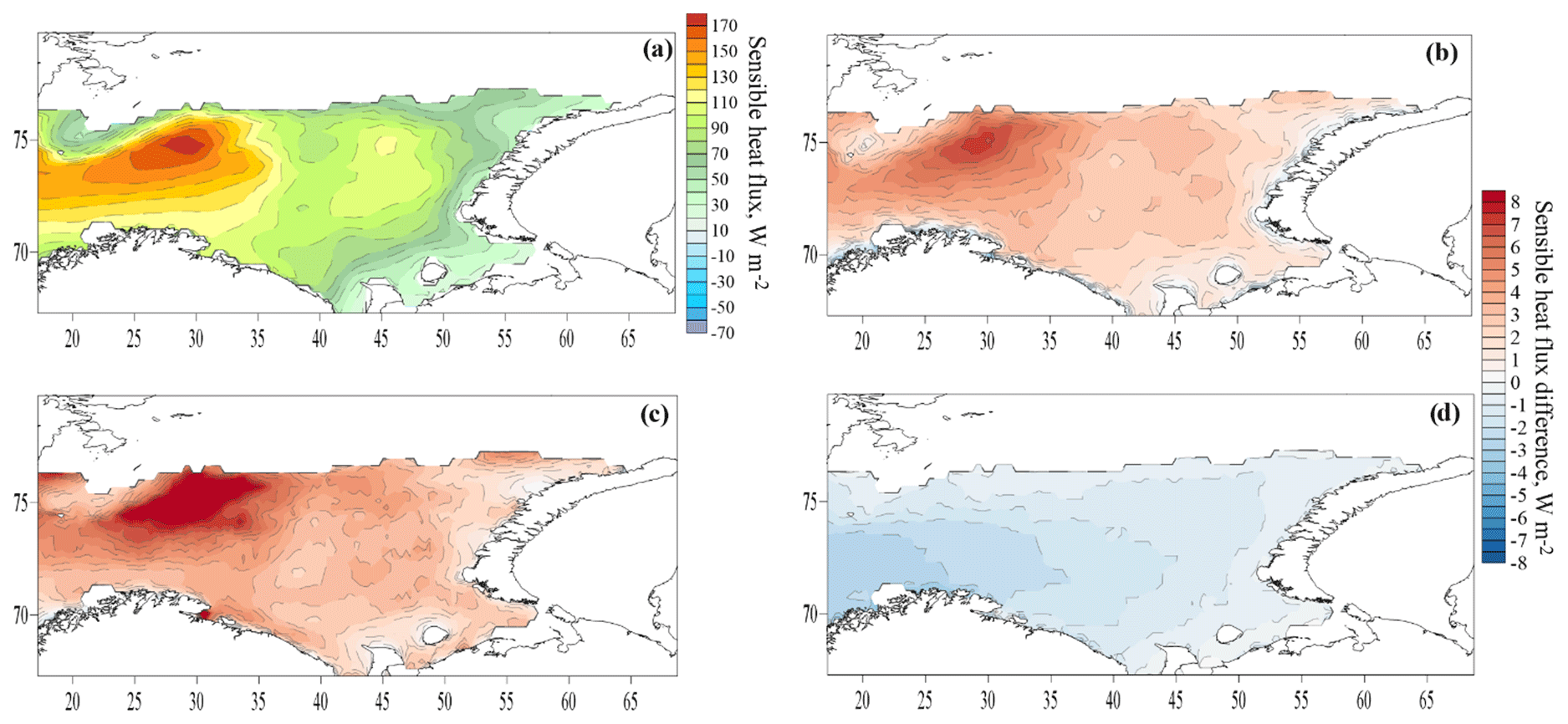
Figure 18 Mean sensible heat flux in experiment C55 (a) and the flux difference in experiments T1–C55 (b), O2–C55 (c) and D3–C55 (d) during simultaneous storms and cold-air outbreaks.

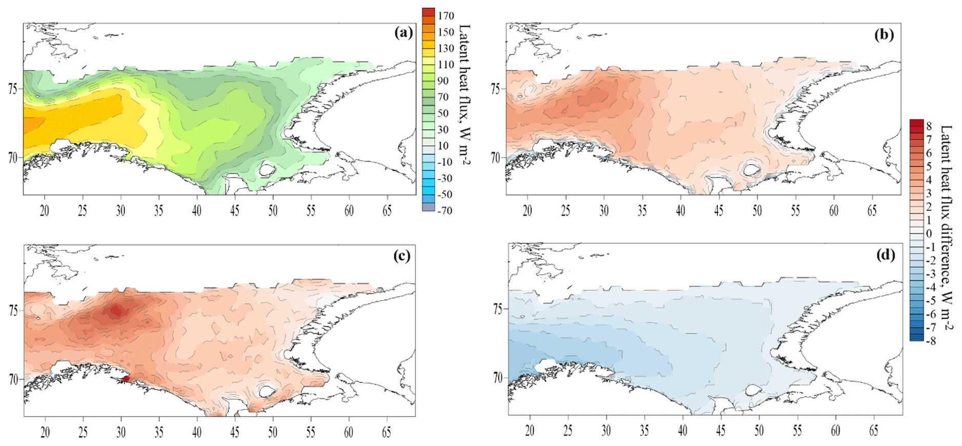
Figure 19 Mean latent heat flux in experiment C55 (a) and the flux difference in experiments T1–C55 (b), O2–C55 (c) and D3–C55 (d) during simultaneous storm wave events and cold-air outbreaks.

4 Discussion and conclusions

This paper presents the results of turbulent heat flux calculations in the Barents Sea using the COARE algorithm, meteorological data from reanalysis and sea wave data from retrospective simulations with the WWIII wave model. The calculations were performed for several options: using the modified Charnock parameterization of roughness length (C55) and explicitly accounting for the sea wave parameters in the T1 (Taylor and Yelland, 2001), O2 (Oost et al., 2002) and D3 (Drennan et al., 2003) roughness parameterizations. Particular attention was paid to the episodes with extremely intense energy exchange between the atmosphere and the ocean: storms and cold-air outbreaks (CAOs).

We obtained the mean annual distribution of the wave height and wavelength in the Barents Sea from wave modeling results. Estimates of the storm activity from 1979 to 2017 were also obtained, confirming its high interannual variability. Based on the wave modeling data, a catalog of storm waves with the wave height exceeding 5 m was created. This catalog was used to calculate heat fluxes during storms.

The catalog of extreme CAOs over the Barents Sea was also obtained. It is shown that the extreme CAOs are observed on 16.4 % of days during a cold season (November–April). However, the number of CAO days varies from 6 in 2011–2012 to 56 in 1981–1982, manifesting large interannual variability. The important role of CAOs in the energy exchange of the Barents Sea and the atmosphere is demonstrated. A high correlation was found between the number of CAO days and the turbulent fluxes of sensible and latent heat, as well as with the net flux of longwave radiation averaged over the ice-free surface of the Barents Sea during a cold season. Thus, the significant interannual variability of the frequency of occurrence of CAOs largely determines the interannual variability of heat loss from the ice-free surface of the Barents Sea.

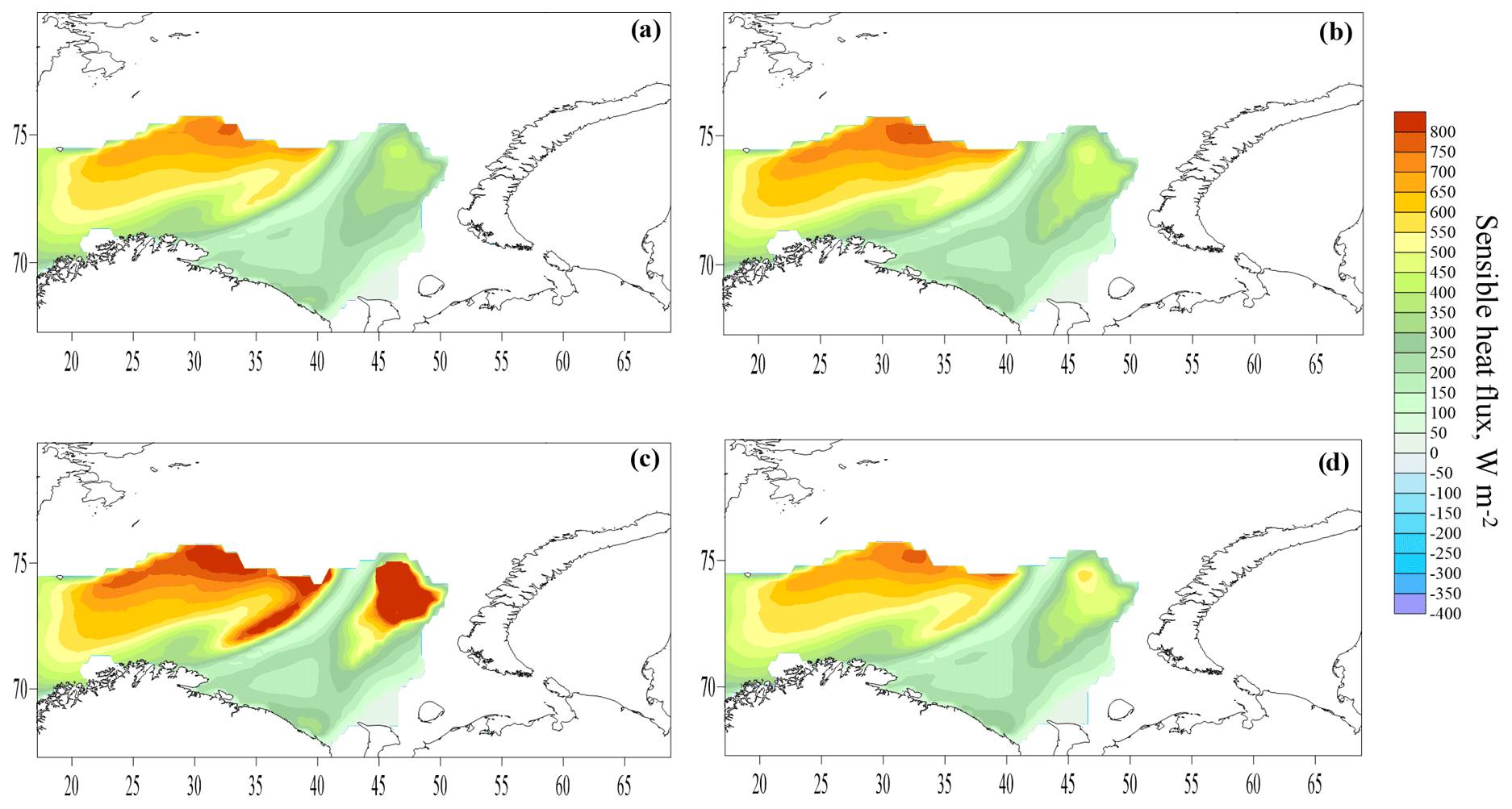
Figure 20 Sensible heat fluxes at 00:00 UTC on 13 January 2003 calculated with the C55 (a), T1 (b), O2 (c) and D3 (d) parameterizations.

Figure 21 Mean relative difference in sensible heat flux (%) in the T1–C55 experiments for all cases (a), during cold-air outbreaks (b), during storms (c),  and during simultaneously observed storm wave events and cold-air outbreaks (d).

Comparison of the calculated heat fluxes with ship observations during the NABOS expeditions was carried out. A significant part of the errors in determining the heat fluxes is associated not with the COARE algorithm used, but with discrepancies in meteorological parameters reproduced by the CFSR reanalysis and locally observed on the ship. We estimated the algorithm error as 4 W m⁻² for sensible heat flux and 8 W m⁻² for latent heat flux, which is within the accuracy of the eddy-covariance method during ship measurements.

The differences between the experiments (long-term calculations for the 1979–2017 period) with different parameterizations of the roughness length are small and are on average 1 %–3 % of the flux magnitude. In some cases, differences can reach 100–200 W m⁻². Parameterizations of Taylor and Yelland (2001) and Oost et al. (2002), which represent the dependence of the roughness length on wave steepness and wave length, respectively, overestimate the magnitude of the fluxes on average, and the parameterization of Drennan et al. (2003) (the dependence of the roughness length on wave height and wave age) steadily underestimates the magnitude of the fluxes over the entire sea compared with the Charnock parameterization. Thus, the effect of explicitly accounting for wave parameters is small when time averaging is performed and is multidirectional, depending on the parameterization used. The modified Charnock formula quite successfully describes the real behavior of the surface roughness even without explicitly taking the wave parameters into account. This can be explained, firstly, by the Charnock parameter's dependence on various ranges of wind speed obtained from empirical data, and secondly, by the high correlation between wave parameters and wind speed that is usually observed. Therefore, in climate studies operating with large timescales and spatially and temporally averaged values, it can be argued that explicitly accounting for sea waves in the calculations of heat fluxes can be neglected. This conclusion is based on long-term calculations and applies exclusively to the Barents Sea. The differences will be even smaller in the tropical or the equatorial regions, as there is low storm activity. In the middle latitudes, the influence of waves on the heat fluxes would require an additional research.

However, in some situations, the choice of a particular roughness parameterization may be important. During storms and cold-air outbreaks, differences between parameterizations increase along with the turbulent heat transfer increase. In some extreme cases, during storms and cold-air outbreaks, the T1–C55 difference reaches 100 W m⁻², and the O2–C55 difference exceeds 700 W m⁻². The O2 parametrization gives the highest values of heat fluxes and roughness length among other parameterizations, and in some cases (in cases of very young sea), calculated values do not correspond to reality; for instance, sensible heat flux reached 1300 W m⁻² and the roughness length reached 7 m in the case shown on Fig. 20. For the same case, the roughness length reached only 2 mm in the C55 calculations, 1 cm in the T1 calculations and 5 cm in the D3 calculations. Although the D3 parametrization depends on the wave age as well as the O2 parametrization, the degree of dependence in the former is lower than that in the latter.

The difference between the experiments with the D3 and C55 parameterizations is almost the same in all cases and always decreases (modulo) from west to east of the sea, actually resembling the mean distribution of wave height. Experiments with parameterizations T1 and O2 deviate most strongly from the Charnock parametrization in those areas and at those times when the absolute values of the fluxes are large. The greatest absolute difference between the fluxes is obtained for the simultaneous action of storms and cold-air outbreaks in the northwest and northeast of the sea, i.e., when the values of the fluxes are the greatest and sea state is young. The relative flux difference (the difference normalized to the value of the flux) over the entire sea is greatest during storms (in some areas more than 5 %) (Fig. 21), but in some areas (in the north, near the ice edge) the relative difference is higher due to the simultaneous action of cold-air outbreaks and storms. In all situations, the relative difference is large in the region of the Pechora Sea due to the low absolute values of the fluxes. An area of low absolute and relative flux difference values is located to the northeast of Bear Island.

Finally, based on the results of our study, we can recommend the use of the parameterizations that consider the wave parameters explicitly on small timescales, for example, in weather prediction, in the Barents Sea region. This is especially true in the case of the simultaneous action of storms and cold-air outbreaks and in the case of relatively short fetches and a young sea state. However, we cannot recommend any particular parametrization due to the lack of in situ observations in the situations where the heat flux differences between parameterizations are large. Our results highlight the fact that one should be cautious when using the Oost et al. (2002) parametrization in young sea state conditions.

All of the conclusions made are valid when turbulent heat fluxes are under consideration. Obviously, differences in the roughness length between calculations with different parameterizations have a more explicit and strong effect on the momentum flux. Although the latter was not the object of this study, its values were nevertheless estimated, and mean relative differences in momentum flux between the parameterizations reached 100 % of the flux magnitude. Thus, the choice of the parametrization is a key factor in the momentum air–sea exchange applications.