the Creative Commons Attribution 4.0 License.
the Creative Commons Attribution 4.0 License.
 | 07 Apr 2021
Identification of atmospheric and oceanic teleconnection patterns in a 20-year global data set of the atmospheric water vapour column measured from satellites in the visible spectral range
Steffen Beirle
Steffen Dörner
Christian Borger
Roeland Van Malderen
We used a global long-term (1995–2015) data set of total column water vapour (TCWV) derived from satellite observations to quantify to which extent the temporal patterns of various teleconnections can be identified in this data set. To our knowledge, such a comprehensive global TCWV data set was rarely used for teleconnection studies. One important property of the TCWV data set is that it is purely based on observational data. We developed a new empirical method to decide whether a teleconnection index is significantly detected in the global data set. We compared our new method to well-established hypothesis tests and found good agreement with the results of our approach. Based on our empirical method more than 40 teleconnection indices were significantly detected in the global TCWV data set derived from satellite observations. In addition to the satellite data we also applied our method to other global data sets derived from ERA-Interim. One important finding is that the spatial patterns obtained for the ERA TCWV data are very similar to the observational TCWV data set indicating a high consistency between the satellite and ERA data. Moreover, similar results are also found for two selections of ERA data (either all data or mainly clear-sky data). This finding indicates that the clear-sky bias of the satellite data set is negligible for the results of this study. However, for some indices, also systematic differences in the spatial patterns between the satellite and model data set were found probably indicating possible shortcomings in the model data. For most “traditional” teleconnection data sets (surface temperature, surface pressure, geopotential heights and meridional winds at different altitudes) a smaller number of significant teleconnection indices was found than for the TCWV data sets, while for zonal winds at different altitudes, the number of significant teleconnection indices (up to > 50) was higher. The strongest teleconnection signals were found in the data sets of tropospheric geopotential heights and surface pressure. In all global data sets, no “other indices” (solar variability, stratospheric AOD or hurricane frequency) were significantly detected. Since many teleconnection indices are strongly correlated, we also applied our method to a set of orthogonalised indices, which represent the dominant independent temporal teleconnection patterns. The number of significantly detected orthogonalised indices (20) was found to be much smaller than for the original indices (42). Based on the orthogonalised indices we derived the global spatial distribution of the cumulative effect of teleconnections. The strongest effect on the TCWV is found in the tropics and high latitudes.
- Article
(59120 KB) - Full-text XML
- BibTeX
- EndNote


It has been known for a long time that weather at one location can be linked to weather at a far distant location (Walker and Bliss, 1932; Bjerknes, 1966, 1969; Wallace and Gutzler, 1981; Nigam and Baxter, 2015; Feldstein and Frantzke, 2017, and references therein). The distances between such locations can be very large, up to opposite locations on the globe. The strength of the correlation varies with location exhibiting regions of maximum (anti-)correlations and regions without any significant correlation. The resulting correlation patterns are referred to as teleconnection patterns. The strongest teleconnection is the El Nin̄o–Southern Oscillation (ENSO) phenomenon (Walker and Bliss, 1932; Bjerknes, 1966, 1969), but many more teleconnections are known, which are located in many regions in both hemispheres (e.g. Feldstein and Frantzke, 2017, and references therein).
The temporal variability of teleconnections is usually described by teleconnection indices (e.g. the ratio of surface pressures at selected stations) and covers a wide range of frequencies from a few days to inter-annual and inter-decadal timescales (Hurrel, 1995; Feldstein, 2000; Nigam and Baxter, 2015; Woolings et al., 2015; Feldstein et al., 2017). Atmospheric teleconnections (e.g. the North Atlantic Oscillation, NAO) have typically higher intrinsic frequencies than oceanic teleconnection indices (e.g. the Atlantic Meridional Mode, AMM).
Teleconnections can be identified in different data sets like sea level pressure, surface air temperature, sea level pressure, as well as geopotential heights and wind fields at different altitudes (Wallace and Gutzler, 1981; Thompson and Wallace, 1998; Nigam and Baxter, 2015; Feldstein and Frantzke, 2017). In recent studies, the geopotential height is the most used variable for the quantification of teleconnections. Teleconnections are mainly found in the troposphere with the strongest amplitudes in the upper troposphere (Feldstein, 2000). But several teleconnections also have connections to the stratosphere (Feldstein, 2000, and references therein; Nigam and Baxter, 2015; Feldstein and Frantzke, 2017; Domeisen et al., 2019). Teleconnections can be identified and defined in different ways: historically, teleconnection indices were empirically and intuitively determined based on the locations of meteorological stations (e.g. Walker and Bliss, 1932). In later studies more objective methods were developed based on correlation matrices, principle component analyses (PCAs) (also referred to as empirical orthogonal function (EOF) methods) or rotated PCAs (also referred to as varimax rotation). More details about these and further methods can be found in Horel (1981), Wallace and Gutzler (1981), Barnston and Livezey (1987), Thompson and Wallace (1998), Feldstein and Frantzke (2017) and references therein. If these methods are applied, the derived teleconnection time series and spatial patterns particularly depend on the selected region of the globe. Most of such studies use pressure or geopotential heights and are confined to midlatitude and Arctic regions in the Northern Hemisphere because of the barotropic conditions in the tropical latitudes. Thus usually, these methods are not applied for the full globe.
Besides the fact that teleconnections are interesting in themselves, their study is also important for other applications. For example, taking teleconnections into account can improve weather forecasts (Feldstein and Frantzke, 2017, and references therein). They have impact on extreme events, e.g. heat waves, droughts, and floods (King et al., 2016; Yeh et al., 2018, and references therein) and can affect storm tracks. In addition to atmospheric quantities (e.g. humidity, precipitation, stratospheric ozone), teleconnections also affect oceanic variables (e.g. Arctic and Antarctic sea ice, the Atlantic thermohaline circulation) and the marine and terrestrial ecosystems (Feldstein and Frantzke, 2017, and references therein). Finally it is worth noting that teleconnections are expected to change in a changing climate (e.g. King et al., 2016; Feldstein and Frantzke, 2017; Yeh et al., 2018).
In this study we investigate to which extent the temporal patterns of various teleconnections can be identified in the global distribution of the total column water vapour (TCWV). For that purpose we use a consistent long-term data set (1995–2015) derived from satellite observations in the visible spectral range obtained from GOME on ERS-2, SCIAMACHY on ENVISAT and GOME-2 on MetOp (Beirle et al., 2018). The data sets consist of monthly mean values on a latitude–longitude grid, which were carefully merged making use of the long overlap time between the different satellite data sets (for details see Beirle et al., 2018). Validation by independent data sets showed a smooth temporal variation with a stability within 1 % over the whole period (1995–2016) (Danielczok and Schröder, 2017). To our knowledge, teleconnection studies using water vapour data sets are rare (e.g. van Malderen et al., 2018). One particular specialty/advantage of our study is that we use for the first time a global data set which is entirely based on measurements. Here it is important to note that the TCWV is dominated by the atmospheric layers close to the surface. Another important aspect of our study is the development of a new empirical method to decide whether a teleconnection (index) can be significantly identified in an atmospheric data set or not.
Our study addresses the following main questions:
- a.
Which teleconnection indices (and other time series such as indices of solar activity) can be significantly identified in the satellite TCWV data set (or other data sets)? Here it should be noted that with significance we do not mean that an index is significantly detected everywhere on the globe. We are rather interested in whether an index is significantly detected somewhere on the globe, which is usually referred to as “field significance” (see e.g. Wilks, 2006). We also do not aim to identify causal relationships or even to predict the TCWV based on teleconnection indices.
- b.
Are the same results obtained for TCWV data from observations and models? Here also the question is addressed of how representative the satellite observations (for mainly clear sky) are of all sky data sets. Another important aspect is to compare the spatial patterns obtained for the different teleconnections between the satellite and model data sets. Differences in the spatial patterns can give hints on possible shortcomings of the model simulations or measurements.
- c.
How does the number of significant teleconnections in the global TCWV data sets compare to similar results obtained for “traditional” teleconnection data sets like surface temperature, sea level pressure or wind fields, and geopotential heights at different altitudes? From this comparison we can conclude whether our global TCWV data set is suited for teleconnection studies. One advantage of the use of this TCWV data set is that it is exclusively derived from measurements.
- d.
What is the spatial distribution of teleconnection patterns found in the global TCWV distribution? One motivation for this question is that the different teleconnections have specific drivers (e.g. tropical convection). Thus the obtained spatial distributions can give hints on the underlying mechanisms.
The paper is organised as follows: in Sect. 2 the global data sets used in this study are introduced, and in Sect. 3 the considered (mostly teleconnection) indices are described. Section 4 presents the fit function of the indices to the global data sets and the obtained global patterns. In Sect. 5 a new method for the determination of the significance is introduced, which is applied to the different global data sets in Sect. 6. In Sect. 7 a reduced set of orthogonalised teleconnection indices is extracted and. Section 8 presents the global distribution of the cumulative effect of the teleconnections.
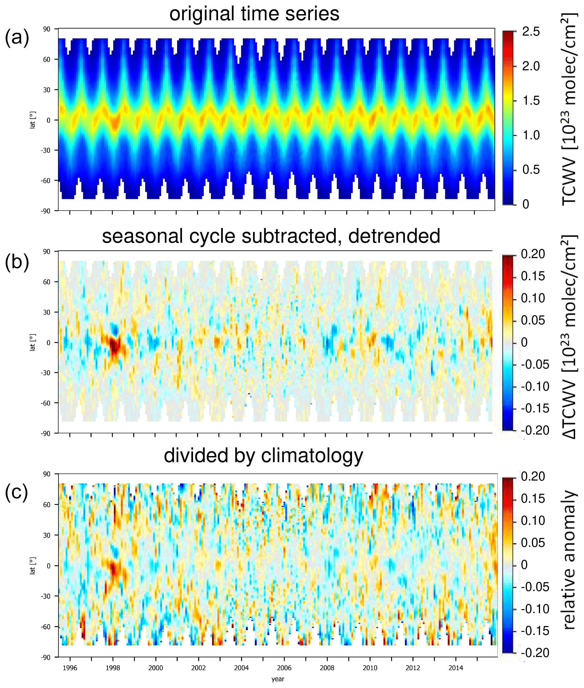
Figure 1(a) TCWV measured from satellite as a function of time and latitude (zonally averaged values) on a latitude–longitude grid with monthly resolution; (b) (absolute anomalies) after the mean seasonal cycle and a linear trend was subtracted; (c) relative anomalies (absolute anomalies divided by the corresponding monthly mean TCWV).
2.1 Total column water vapour
Our study focuses on global long-term data sets of the total column water vapour (TCWV). Here we use three data sets:
- a.
Satellite observations from July 1995 to October 2015 (Beirle et al., 2018) are derived from the satellite instruments GOME on ERS-2 (1995 to 2003), SCIAMACHY on ENVISAT (2002 to 2012) and GOME-2 on MetOp (2006 to present), which have similar overpass times (between 09:30 and 10:30 LT). The data analysis is performed in the red spectral range. Since these satellite instruments observe scattered and reflected sunlight, the observations are sensitive for the whole atmospheric column including the surface-near layers which usually contain the largest fraction of the total atmospheric TCWV. The start date of the time series was predetermined by the start of the first satellite mission; the end date of the time series was set to October 2015, because some of the used time series were only available until that date. The data set is available on a latitude–longitude grid with monthly resolution. The data set does not cover polar winter, since the satellite observations use scattered and reflected sunlight. It should be noted that the satellite data set used in this study was optimised with respect to temporal stability, which makes it well-suited for climate studies. However, because of the rather simple analysis approach, for specific situations small systematic biases of the absolute values might occur, e.g. related to the effects of surface albedo or terrain height. It should also be noted that the satellite data set has some gaps over high mountains (due to the simplified cloud filter) and north of India (because of routine internal calibration measurements of the GOME instrument over that region).
In Fig. 1 the variation of the TCWV with latitude and time is shown (the latitude bins represent zonally averaged values). The top panel shows the original TCWV data set, whereas both lower panels present the absolute and relative anomalies with the mean seasonal cycle removed. Several anomaly patterns are clearly obvious, which are mainly related to strong ENSO events (see e.g. Soden, 2000; Simpson et al., 2001; Wagner et al., 2005). Especially for the relative anomalies, many high-frequency variations are found. While part of these high-frequency variations represent measurement noise and atmospheric noise, the results of this study showed that they also represent atmospheric teleconnections.
In addition to the satellite observations of the TCWV we also use global time series of the TCWV derived from ECMWF reanalysis (ERA Interim, Dee et al., 2011). The main purpose of using model data is that we want to see if teleconnections are found in a similar way in both satellite and model data sets. In addition, the use of model data also allows the quantification of a possible clear-sky bias in the satellite observations, because these observations are made for mainly cloud-free conditions. Therefore we use two model data sets:
- b.
All ERA data including clear and cloudy conditions are used.
- c.
Only ERA data for clear sky observations are used. Here, a cloud cover below 0.3 between 1 and 6 km is regarded as cloud free. This criterion reflects the observational conditions of the satellite data set.
Both data sets have a temporal resolution of 6 h. For the comparison with the satellite TCWV results, the ERA data were temporally interpolated to the time of the satellite overpass (10:00 LT). From the comparison of the results for the measurements and model data sets, the effect of the specific sampling of the satellite observations observing mainly cloud-free situations can be investigated. The application of the cloud filter leads to a reduction of the number of considered model data of about 40 %. In Fig. 2 the global mean distributions of the TCWV data sets from satellite observations and ERA data are shown. Similar patterns are found in all three data sets indicating the good consistency amongst them. The highest values are found over the tropics, especially over the western Pacific. Lower values are found towards higher latitudes showing the strong dependence of the TCWV on temperature.

Figure 2Global mean distribution of the TCWV from satellite observations (a) and ERA data: (b) all data; (c) only clear sky observations during day.
2.2 Other global data sets
Teleconnections patterns are usually derived from meteorological quantities like surface pressure and temperature or geopotential heights and wind fields at different altitudes. In this study we also consider such quantities, which we also obtained from ERA data (see Table 1). We analyse these data sets similarly to the TCWV data sets (details are described below). In this way we will assess in how far the impact of teleconnections on TCWV is comparable to traditional teleconnection data sets.
We performed an extensive search for teleconnection indices in the scientific literature and websites of national weather services. We found in total 54 teleconnection indices, which cover the time span of our TCWV data set. An overview on these teleconnection indices as well as additional time series (e.g. of the solar activity) is given in Table 2. Here it should be noted that for some of these indices with low frequencies (e.g. MGII or IPO) no full period is covered by our 20-year-long satellite TCWV data set, which might be one reason why they are not significantly detected.
Although we not only focus on teleconnection indices in this study, in the following we use the term “index” to describe the whole set of teleconnection indices and other time series.
Table 1Meteorological data sets used in this study.
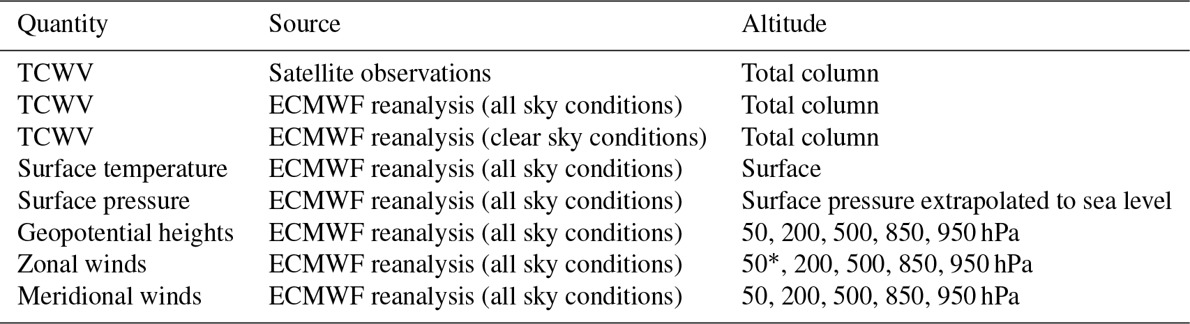
∗ The zonal winds at 50 hPa are not further analysed, because they are – by definition – dominated by the Quasi-Biennial Oscillation (QBO) teleconnection signal.
Table 2Teleconnection indices and other time series used in this study. More details about these indices as well as their sources are given in Fig. A6 in the Appendix.
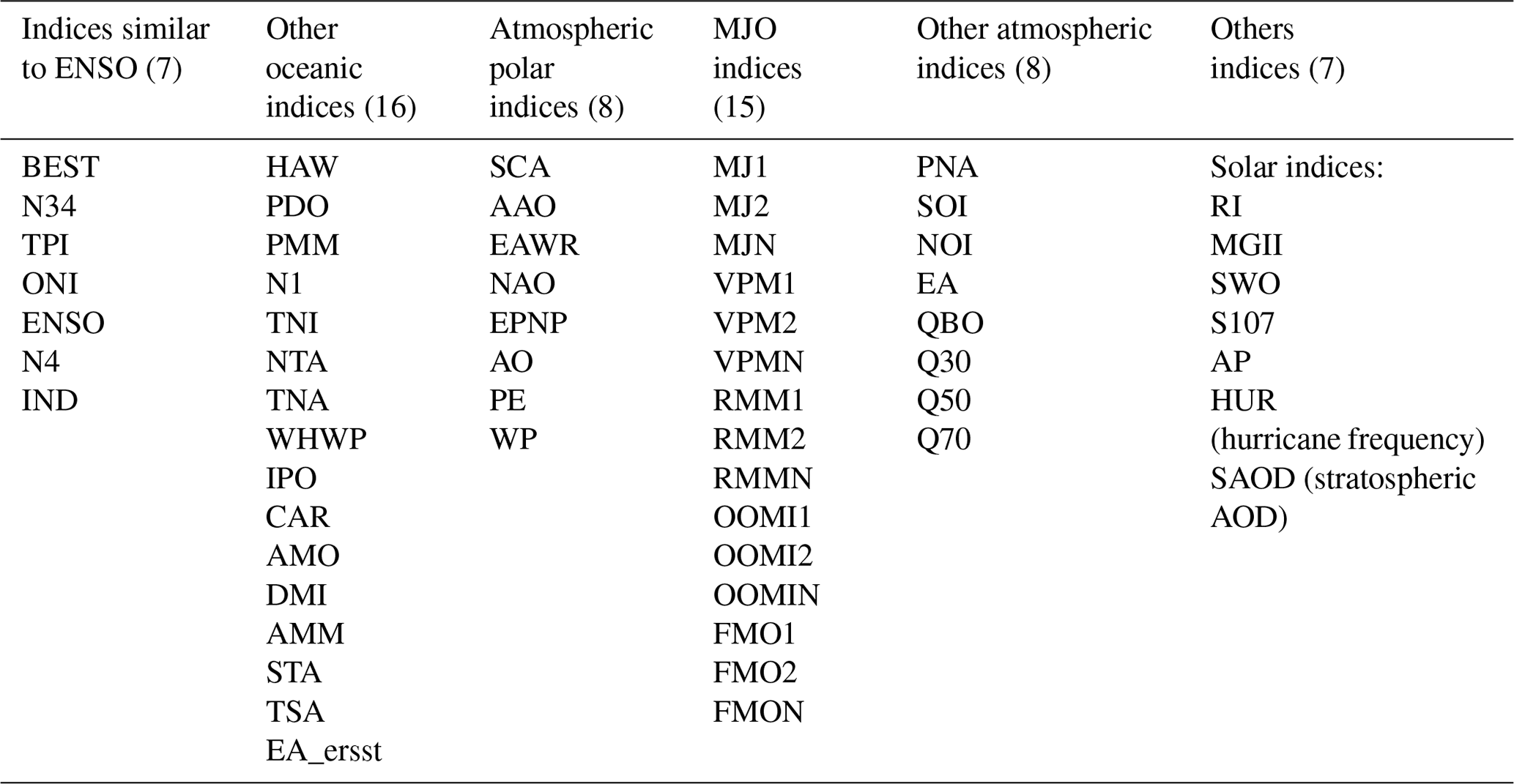
It should be noted that for several teleconnection indices (in particular for the Madden–Julian Oscillation) different definitions exist. Thus the number of teleconnection indices in Table 2 is much larger than the corresponding atmospheric phenomena. Many of these indices (describing the same phenomenon) as well as many of the other teleconnection indices are highly correlated. The strength of these correlations is presented in Fig. 3 as a matrix with correlation coefficients between the different indices (after the seasonal cycles were removed). In spite of the correlations amongst the teleconnection indices, we decided as a first step to include them all in our study, because beforehand it is not clear which index might be best suited to represent a teleconnection phenomenon. Using our empirical approach, however, it becomes possible to quantify the significance and strength of the different indices and thus to select the best suited index for a given teleconnection phenomenon. Finally, we apply an orthogonalisation for the most significant indices (see Sect. 7) to minimise the effect of the correlations and to identify the dominant temporal teleconnection patterns in our TCWV data set.
A detailed overview on the selected indices and their data sources is provided in Fig. A6 in the Appendix.
To determine the strength with which individual indices are detected in the temporal variations of the different global data sets, the index time series are fitted to the global data sets as described in Sect. 4.1 below. Before the fit is applied, the mean seasonal cycle (1995–2015) and a linear trend are subtracted from the individual indices (see e.g. Horel, 1981). Some teleconnection indices are characterised by strong seasonal cycles, whereas others are not. Finally the obtained anomalies are normalised by the corresponding standard deviations. This ensures that the obtained fit coefficients for the different indices can be directly compared. The different steps of these preparations are illustrated in Fig. A7. For consistency, the same steps are also applied to the different global data sets before the fit is applied.
4.1 Fit function
For each latitude–longitude pixel of the global data sets (the example below is for the TCWV) the de-seasonalised time series of the monthly mean anomalies are fitted by the following function:
Here c and b describe constant and linear terms. indexi represents the selected normalised index of monthly mean anomalies. The fit coefficient fi describes the sign and strength of the contribution of the chosen index to the variability of the TCWV anomaly of the chosen pixel. The constant offset c and possible linear trend b and the fit coefficient fi are simultaneously determined by the fit. An example of the derived fit coefficient for the ENSO index is shown in Fig. 4 (top). Systematic patterns with positive and negative fit coefficients are found. The fit function is separately applied to the individual indices listed in Table 2. Here it should be noted that the fit function could in principle be applied to several or even all indices simultaneously. However, since many indices are highly correlated, the interpretation of the results would then not be straightforward. Thus, we chose to include the individual indices one by one in the fit function. Besides the parameters c, b, and the fit coefficient fi, also the difference between the temporal variation of the global data sets and the applied fit function is quantified by the root mean square (rms). The rms for the ENSO index is shown in Fig. 4 (second row).
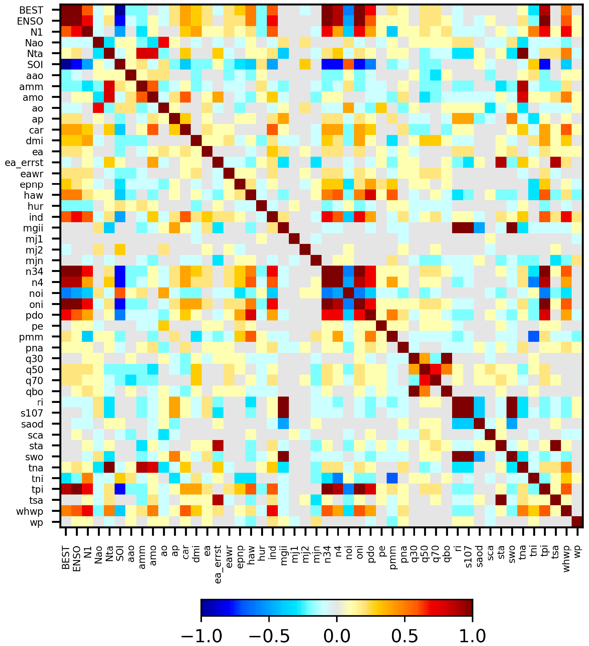
Figure 3Correlation coefficients between the different teleconnection indices (after seasonal cycle was removed). Note that only one set of MJO indices is included here to minimise the total number of indices.
In order to quantify the importance of a selected index, a second fit is performed with only the constant and linear terms:
The comparison of the rms with and without including the index term (Eqs. 1 and 2) allows the quantification of the importance of the chosen index to describe the temporal variation of the data set. Therefore the following quantity is defined:
The rms differences are divided by the zonal mean value (see Appendix A1) of the considered quantity, because (like for water vapour) many of the analysed quantities depend strongly on latitude. The delta rms is a measure for the magnitude of the variance of a considered data set, which can be explained by the chosen teleconnection pattern. If there is high similarity of the temporal variation of an index with the temporal variation of the considered data set, the delta rms is large. If there is no similarity, the corresponding delta rms value is zero.
It should be noted that instead of the delta rms values, also the correlation coefficients between the considered data set and the fit function (Eq. 1) might have been used since the spatial patterns of both quantities are very similar (see Fig. A8).
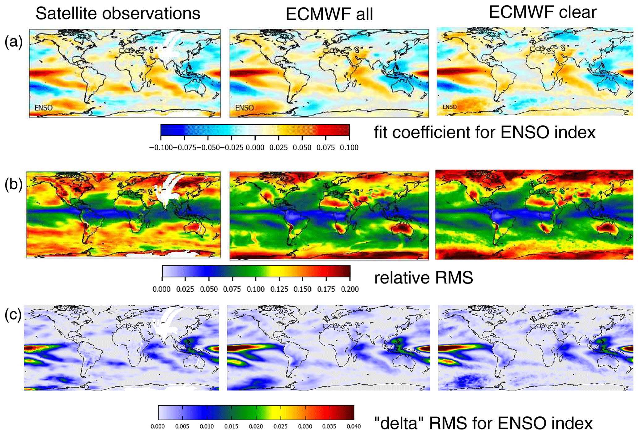
Figure 4Global maps with the ENSO fit results for the three TCWV data sets. (a) Fit coefficients; (b) rms of the differences between original data sets and fit functions; (c) delta rms values which describe the relative difference of the rms if the ENSO index is included or excluded in the fit function (for details see text).
The delta rms value for the ENSO index is also shown in Fig. 4 (bottom).
The fit results in Fig. 4 for the ENSO index are obtained for the TCWV from satellite observations (left), ERA data (centre), and ERA data for clear sky conditions (right). High fit coefficients (Fig. 4 top) mean that a substantial part of the measured TCWV time series can be explained by the ENSO index pattern. High negative fit coefficients mean the same for the negative ENSO index. Fit coefficients of zero indicate no connection to ENSO. Very similar spatial patterns are found for the three TCWV data sets indicating that the ENSO phenomenon is well captured in the satellite and model data sets. From the similarity between the model data including all sky conditions (centre) or only clear sky conditions (right), it can be concluded that the satellite observations (representing mainly clear sky conditions) are representative of all sky conditions (no obvious clear-sky bias).
In all three data sets, the smallest rms values (Fig. 4, second row) are found close to the Equator. This is an interesting finding but can probably be explained by (a) the rather high TCWV and (b) its rather small variability in these regions. In mid-latitudes, systematically higher rms values are found for the satellite observations compared to the model results. This is probably related to the rather large effects of clouds on the satellite observations, which becomes especially important in these regions (clouds lead to fewer valid observations and larger measurement uncertainties). Another interesting finding is that in polar regions the rms for the satellite observations is smaller than for the model results. This finding is probably related to the sparseness of water vapour measurements in these regions assimilated in the ECMWF model. Thus the spatio-temporal variability of the satellite observations is probably more realistic than that of the model data. The rms for the model results for clear sky conditions is slightly higher than for the model results for all conditions, which is to be expected because of the reduced number of input data for the cloud-filtered data set (about 40 % less compared to the non-filtered data set).
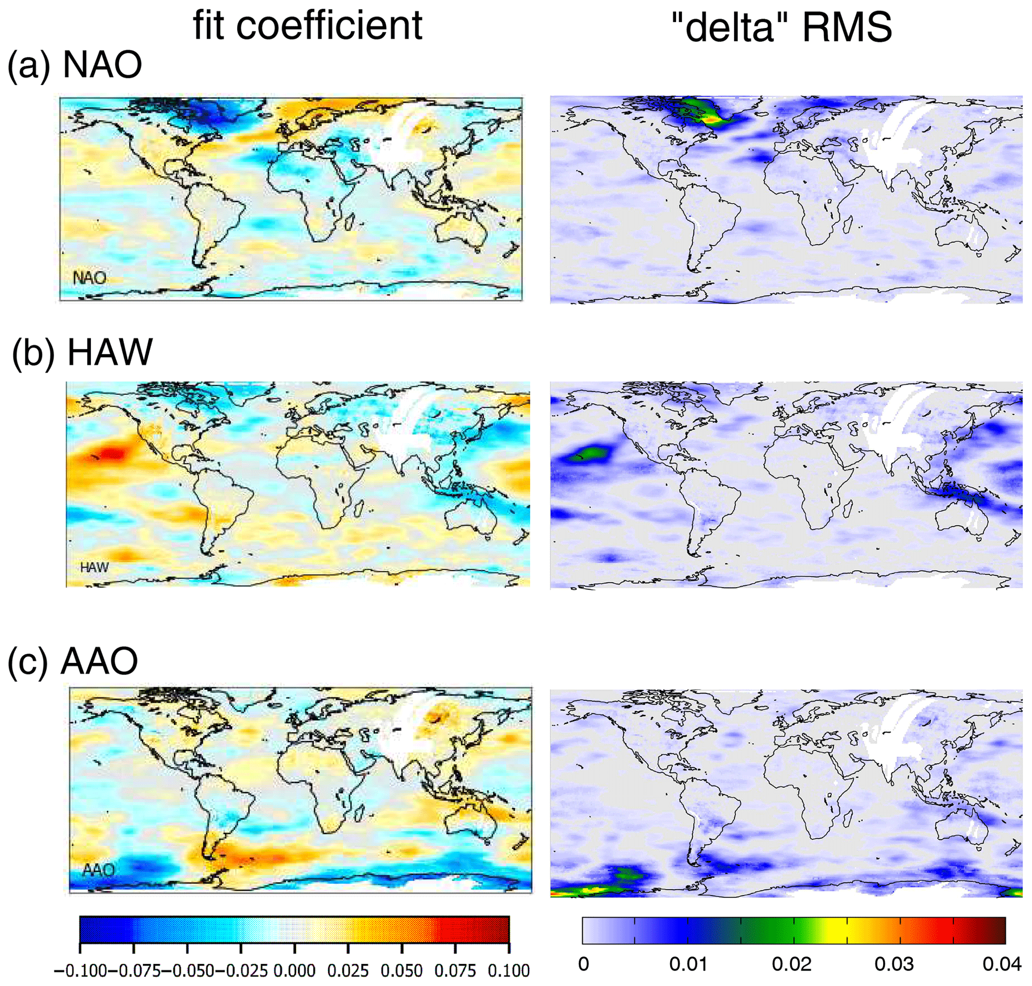
Figure 5Global maps with the fit results (left) and delta rms (right) for selected teleconnection indices with activity centres in northern high latitudes (a), subtropics (b) and southern high latitudes (c). Results for the TCWV data set from satellite observations.
The lower panel of Fig. 4 shows the delta rms for the ENSO index indicating the reduction of the rms if the ENSO index is included in the fit. As expected, the largest delta rms is found over the tropical Pacific, where the ENSO phenomenon is most pronounced. The global distribution of the delta rms is very similar for the three data sets. The fit coefficients and delta rms for three other selected indices are shown in Fig. 5 for the TCWV data set from satellite observations. For all indices, specific activity centres can be found in different parts of the globe. The fit coefficients for all indices are presented in the Appendix (Fig. A9). Note that in general very similar spatial patterns are found for the three TCWV data sets, but in some cases also systematic differences are derived (for more details see Sect. 6.1). As expected, for groups of indices with strong temporal correlation also similar spatial patterns are found. This is most obvious for indices similar to the ENSO index (first group of indices in Figs. A6 and A8). Similar spatial patterns are also found for other pairs of indices, e.g. between the Hawaiian Index (HAW) and the Pacific Decadal Oscillation (PDO) as well as between the South Tropical Atlantic Index (STA) and the Equatorial Atlantic Index (EA_errst).
For most teleconnection indices spatially coherent patterns of fit coefficients and delta rms values are found in the global maps (see Fig. A9) indicating that these indices are significantly detected in the global water vapour data sets. These spatial patterns agree also well with the known regions where the corresponding teleconnections are active. Information about the significance of the fit results can be obtained from the fit function itself. However, in practice, the significance information from the fit has several limitations:
- a.
The determination of the significance is based on several assumptions about the data sets (e.g. that all data points of the time series have the same uncertainties and follow a normal distribution). However, the errors of the individual data points can be very different. For example the effect of clouds on the errors of the satellite TCWV data set can be very different for different seasons and regions. Also, the uncertainties are not only random but contain also systematic contributions. It is difficult (if not impossible) to quantify the uncertainties of the involved time series.
- b.
The determination of the significance is based on prescribed significance levels. The choice of such a significance level is arbitrary, and the obtained significance information depends on this choice.
- c.
In several tests we fitted artificial time series to the TCWV data set. These tests showed that even for such non-geophysical time series “significant” fit results can be obtained (see the examples in Fig. 6). On the left side of this figure, fit results for a time series containing only white noise, and on the right side fit results for a temporally reversed teleconnection index are shown (the temporally reversed index is obtained from the original index by mirroring the time axis). The blue and red areas show fit coefficients for both time series, which are classified as significant by the fit.
To address these difficulties, we developed and applied an empirical approach to determine threshold values for the delta rms values to decide whether an index is significantly detected in a global data set. The new procedure is described in the next section. It has the following two main advantages:
-
The threshold values are determined empirically. Thus no assumptions on the properties of the time series or the significance levels have to be made.
-
The method provides a clear procedure and in particular a metric which can be applied in a consistent way to different data sets and thus allows a quantitative comparison (see Sect. 6).
We compared the results of our empirical approach to literature hypothesis tests and found good agreement (see Sect. 5.2)
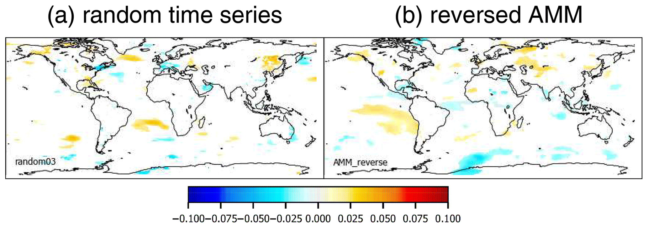
Figure 6Global maps of the fit results for an artificial time series containing only white noise (a) and a temporally reversed teleconnection index (AMM, b). The white areas represent fit results, which are classified as non-significant by the fit routine (for a 5 % significance level).
5.1 Use of reversed indices
The basic idea of our new approach is to use non-geophysical indices for the estimation of the significance level. Non-geophysical indices are indices without any temporal correlation with the temporal variations of the investigated geophysical data sets. For that purpose we chose all temporally reversed indices (see Table 2 and Fig. A6), because they cover all relevant frequencies of the true teleconnections. In practice, the time axis is flipped, which means the first entry (July 1995) will be assigned to the last month (October 2015), and so on. In a first step, we calculate the 99th percentile of the delta rms values of the reversed indices for all pixels of the global map. We chose the 99th percentile because it is close to the maximum but still not affected by individual outliers. Here it should be noted that the exact choice of the percentile is not critical, as the same percentile is applied to both original and reversed indices. We found exactly the same set of significant indices (see below) if we used the 95th percentile or the 98th percentile.
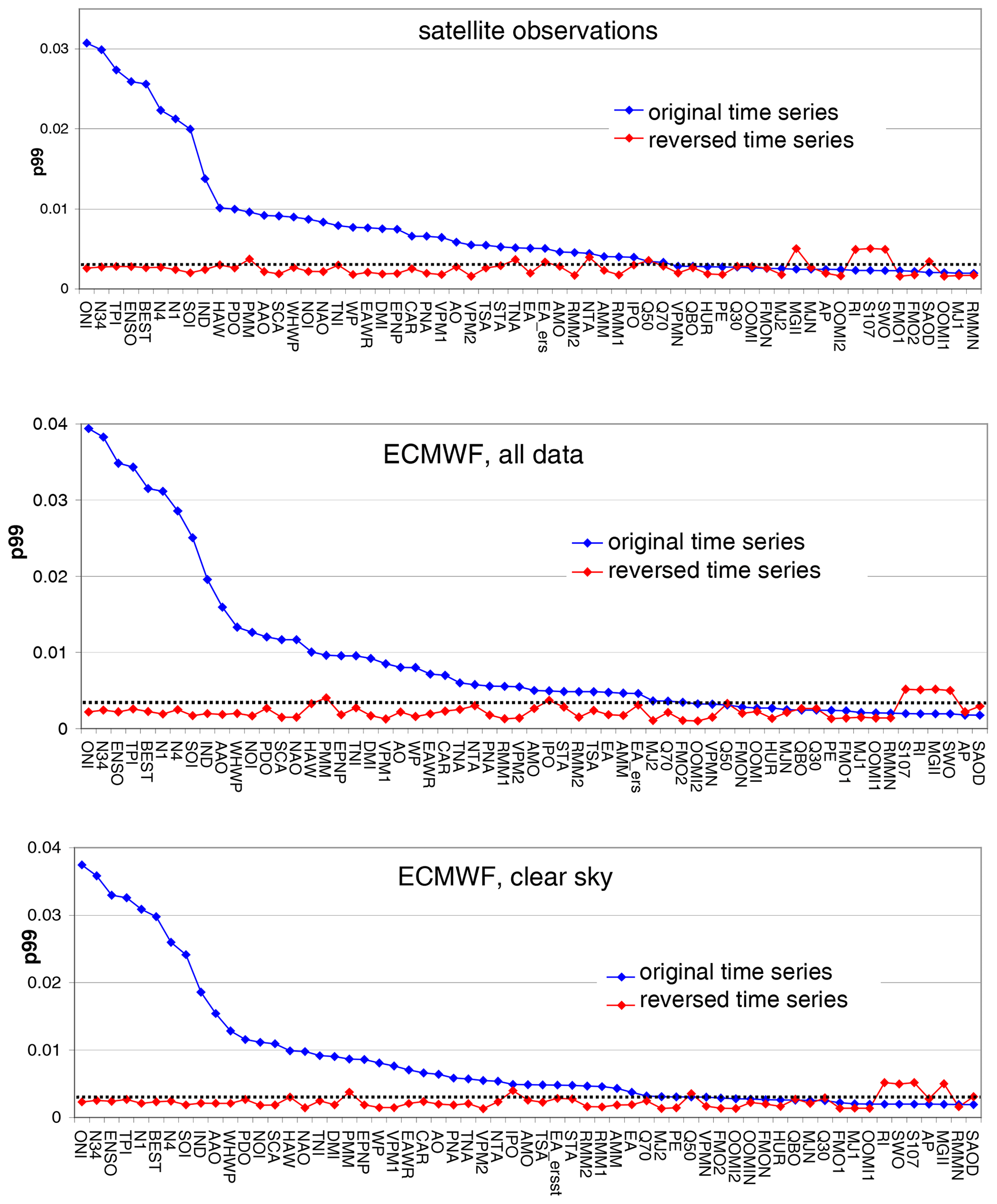
Figure 7Blue markers: 99th percentiles (p99) of the delta rms of the original indices for the three TCWV data sets. Red markers: similar results for the temporally reversed indices. Black lines: significance threshold. The indices are sorted from highest to lowest p99 values for the original indices. Note that different y axes are used for the satellite and model data.
The red data points in Fig. 7 present the 99th percentiles (p99) for all reversed indices for the three TCWV data sets. From the mean value and standard deviation of the results for all temporally reversed indices, we calculate a threshold value (black dotted line in Fig. 7) for each data set (for details see Appendix A2). The obtained threshold value for the TCWV data set from satellite observations is 0.0031. We also applied the same method to a set of 100 artificial random time series and obtained a slightly smaller threshold value of 0.0027 indicating that the threshold value obtained from the temporally reversed time series is reasonable.
If the p99 values are above the threshold, it is likely that the considered index significantly contributes to the variability of the considered data set and vice versa.
In Fig. 7 besides the p99 values for the temporally reversed indices (red), also those for the original indices are shown (blue). For many of the original indices, the p99 values are much larger than the threshold value indicating that these indices are significantly detected in the respective data set.
In addition to the use of the absolute threshold of the delta rms values for the determination of significance, we also made use of the effect of time shifts applied to the individual indices. The underlying idea is that the delta rms values should decrease if the original indices are de-synchronised by ± 1 month. The details of this approach are described in Appendix A3. Using this additional criterion, a few more indices are added to the number of significantly detected teleconnection indices. For the TCWV data set from satellite observations, the number of significantly detected indices increases from 40 to 42, for the ERA TCWV data set from 43 to 44, and for the ERA data set for clear sky conditions from 39 to 42.
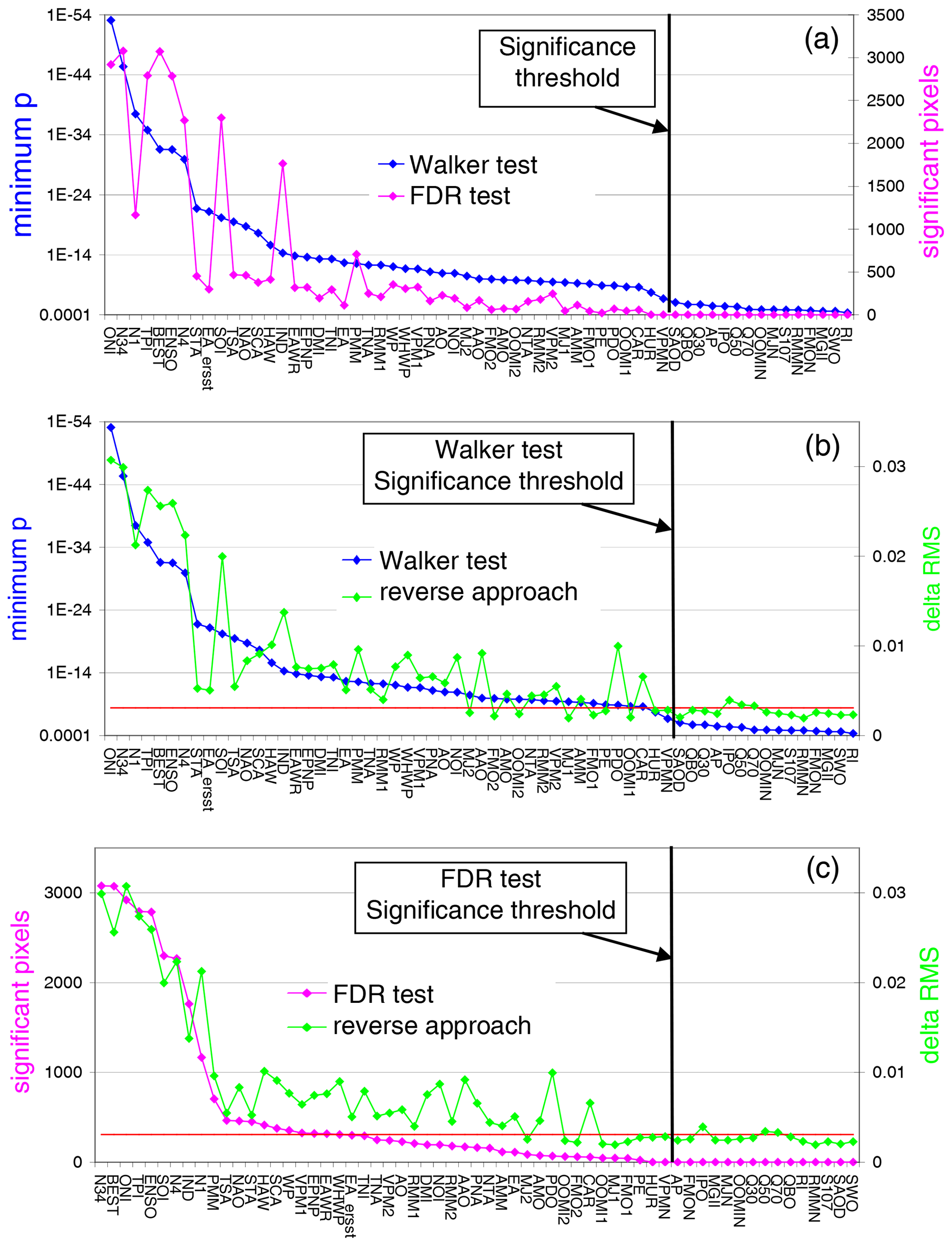
Figure 8Comparison of the results of the three approaches. (a) Results for the Walker test (left axis) and FDR test (right axis) for a significance level of 1 %. The indices are sorted according to the results of the Walker test. The black vertical line indicates the significance threshold (similar for both tests). (b) Comparison of the results for the Walker test (left axis) and our empirical (reverse) approach (right axis). The indices are sorted according to the results of the Walker test. The black vertical line indicates the significance threshold of the Walker test. The red horizontal line indicates the significance threshold for our empirical approach. (c) Similar as for the middle panel, but for the FDR test.
5.2 Comparison of the results from the empirical approach to established tests
We compared the results of our new empirical approach to those of standard methods for significance testing. For this purpose we derived the local p values for each individual fit by a two-tailed t test. As standard methods we applied the so-called Walker test and the false discovery rate (FDR) test (e.g. Wilks, 2006, 2016). The Walker test uses the minimum local p value derived from the individual fits as the global test statistic. The FDR test compares the p values of all grid pixels with the distribution of the statistically expected FDR. Both tests deal with the problem of field significance. Another advantage of both tests is that they are rather robust with respect to spatial correlations. We also account for effects of temporal autocorrelation within the fit method by assuming an AR(1) process of the fit residual (Seabold and Perktold, 2010). We applied both standard tests to the satellite TCWV data set and compared the results to those of our empirical approach using reversed indices (Fig. 8). Especially for the FDR test, very similar results were obtained compared to our empirical approach. Only a few indices with low frequencies (Q50, Q70, and IPO), which were previously found to be slightly above the significance level, are now found to be slightly below the significance level. Conversely, some previously non-significant indices with high frequencies are now found to be slightly above the significance threshold. These changes are related to the fact that for the new method we also accounted for the temporal correlations of the indices. The most important finding, however, is that these differences between the FDR test and the old method are only found for indices close to the significance thresholds and thus do not affect the main findings of our study. The number of significant indices found for our empirical approach and the FDR test differs only by 2 (42 for our empirical method and 44 for the new method) if one takes into account that the OOMI2 and FMO2 as well as the OOMI1 and FMO1 indices are very similar.
Another interesting finding is that for the Walker test and the FDR test exactly the same number of significant indices is found. However, the order of importance obtained from both tests also shows large differences for some indices (Fig. 8 top).
6.1 Comparison of the results for the TCWV data sets to those for the other data sets
A rather high number of significant indices was identified in the global TCWV data sets. To put this finding into a broader perspective, we applied the same procedure also to other global data sets, which are usually considered in teleconnection studies (see Table 1). The corresponding p99 values of the different indices (including also the reversed indices) are presented in Fig. A10. In general similar results as for the TCWV data sets are found. In particular, for all data sets a large number of teleconnection indices is significantly detected. However, also differences are found: in particular, the teleconnection index with the maximum p99 value is found to be different for the different data sets. For the TCWV data sets, surface temperature and pressure, as well as most of the zonal winds, the largest p99 values are found for indices similar to ENSO. For the TCWV data sets and surface temperature, this can be expected, because the ENSO phenomenon is driven by the surface temperature (over the tropical Pacific). Accordingly, also the TCWV data sets will be strongly affected, because the TCWV depends strongly on the temperature in the lowest atmospheric layers. The strong influence of the ENSO phenomenon (BEST index) on the zonal winds at most levels can probably be explained by the fact that large-scale phenomena like ENSO can have a strong influence on the quasi-persistent zonal flow patterns in the tropics and subtropics. For the geopotential heights and meridional winds, the largest p99 values are found for the polar atmospheric indices (mostly AAO, but also SCA). For the geopotential heights this might be expected because the polar atmospheric indices are defined based on anomalies of the geopotential heights. Also for the zonal winds, the largest p99 values are found for the polar atmospheric indices, which is probably caused by the strong relationship between geopotential heights and winds.
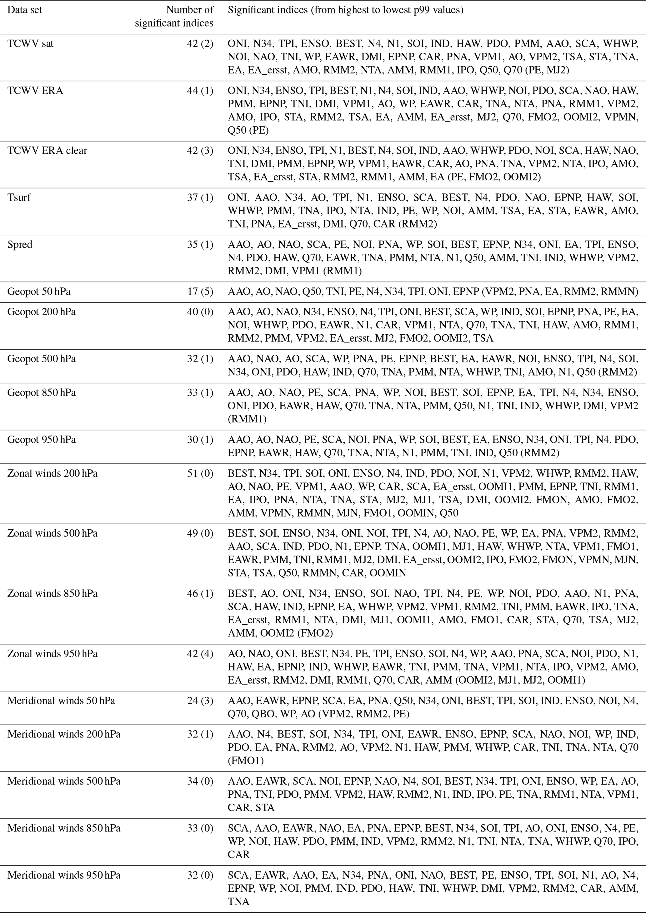
Table 3Numbers of significant indices and most significant indices for all data sets (the number of indices with p99 values below the threshold but with shift ratios < 0.8 are indicated in brackets). The complete list of significant indices for the different data sets is provided in Table A1 in the Appendix.

A summary of the number of significant indices and the teleconnection index with the highest p99 is given in Table 3. Most significant indices are found for the zonal winds with the highest number in the upper troposphere. For these data sets the number of significant indices is larger than for the TCWV data sets. For geopotential heights and meridional winds, fewer significant indices are found (and even less than for the TCWV data sets). For geopotential heights most significant indices are found in the upper troposphere, while for the meridional winds no clear altitude dependence is observed. Also for the surface temperature and surface pressure rather low numbers (less than for the TCWV data sets) of significant indices are found. From these results we conclude that the global TCWV data sets are well suited for teleconnection studies. Here it should again be noted that the satellite TCWV data are exclusively determined from measurements, and the TCWV is dominated by the layers close to the surface. Thus our findings indicate that also indices which are usually detected in the middle and upper troposphere can be significantly detected in data sets which are dominated by the lower troposphere.
Our new method for the determination of the significance level also allows a direct comparison of the strengths at which the different indices are detected in the different data sets. In Table 3 also the maximum p99 values of the delta rms normalised by the corresponding significance threshold values are shown. The highest normalised p99 values are found for the geopotential heights (except the 50 hPa level) and the surface pressure. This finding is consistent with the fact that these quantities are used in most teleconnection studies and many indices are even defined using these quantities. The lowest normalised p99 values are found for zonal winds, for which also the smallest numbers of significant indices are obtained. Intermediate values are found for the water vapour data sets.
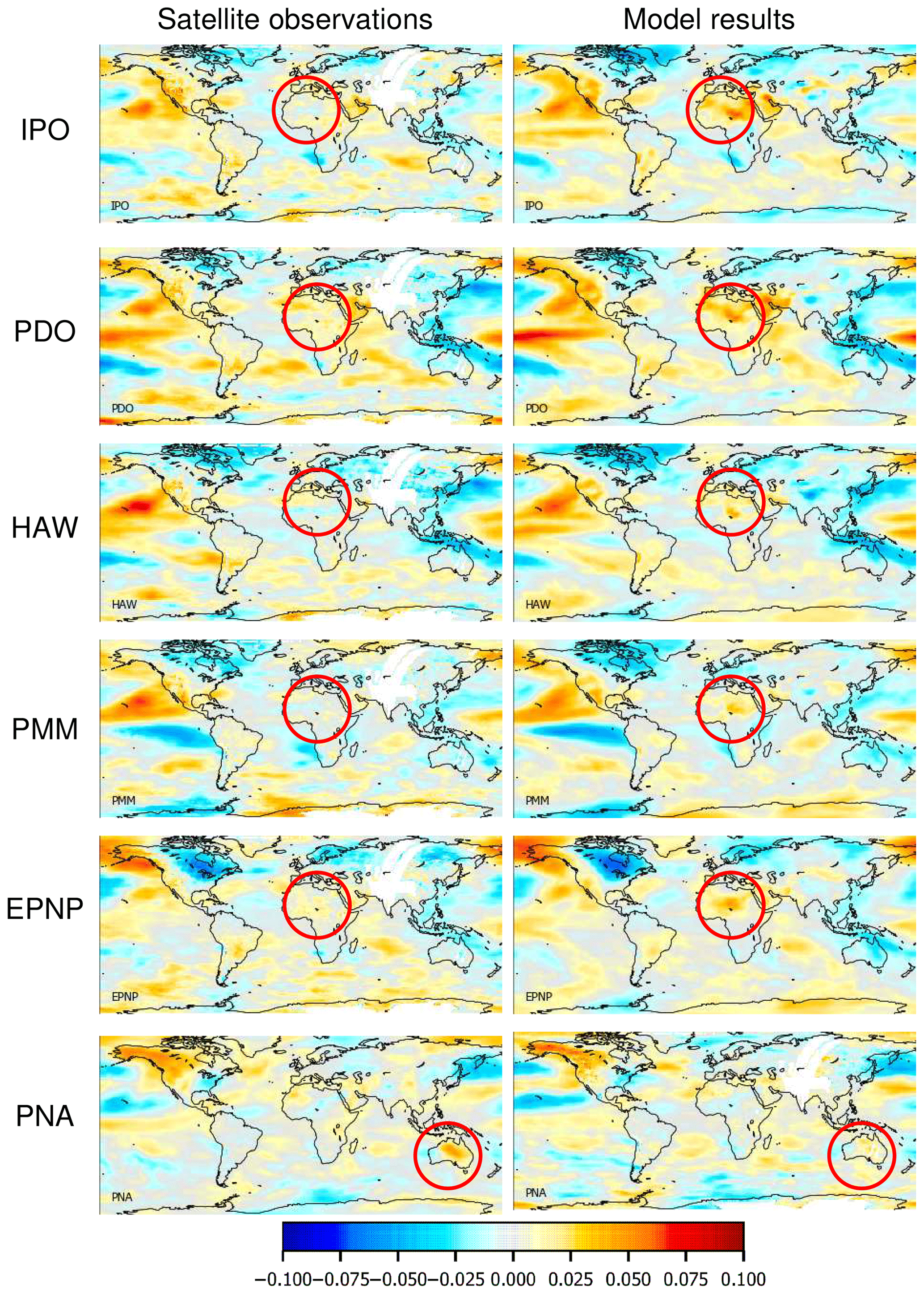
Figure 9Fit coefficients for selected teleconnection indices, for which different patterns were found in the TCWV data set from satellite observations (left) and model simulations (right). The red circles indicate regions with substantial differences between the results for both data sets.
6.2 Comparison of the spatial patterns of the measured and simulated TCWV
For most of the teleconnection indices, very similar spatial patterns are found in the TCWV data sets obtained from satellite or ECMWF data (see Fig. A9). This confirms both the high quality of the satellite measurements and model simulations. However, for some indices, also substantial differences are found (see Fig. 9). The most obvious differences are found over northern Africa. In principle, they could be caused by errors of both the satellite or model data sets. However, since very good agreement over northern Africa is found for most of the indices, we can very probably exclude systematic measurement biases in the satellite data set (e.g. effects from the high surface albedo over the Sahara). Thus we conclude that the observed differences probably indicate deficiencies in the model simulations, possibly related to the sparseness of observational data over northern Africa used in the model. It is interesting to note that the differences are found for both oceanic and atmospheric indices which have rather different frequencies. These comparison results might help to improve the model performance over northern Africa (and to a lesser degree also over other regions).
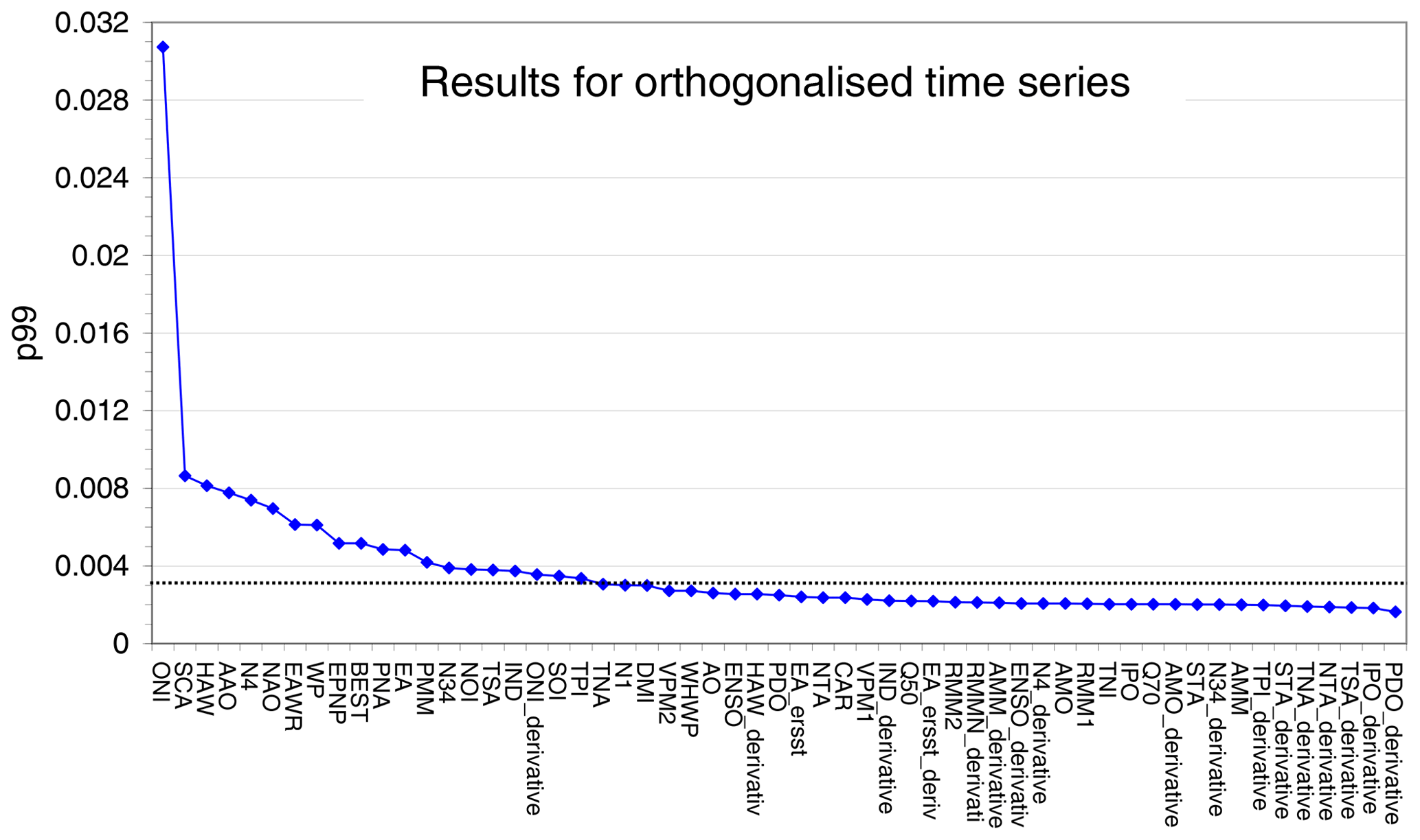
Figure 10The 99th percentiles (p99) of the delta rms of the orthogonalised indices. The black lines represent the significance threshold. The indices are sorted from highest to lowest p99 values.
It was shown in Fig. 3 that many indices are strongly correlated. Thus the numbers of “significant indices” obtained in the previous chapters are not useful to represent the number of independent significant indices. To account for correlations between the different indices, we thus applied an orthogonalisation approach. For the orthogonalisation (based on the Gram–Schmidt process), all “significant” original indices and significant temporal derivatives (see Fig. A11) were considered (in total 57 indices). The order of indices used in the iterative orthogonalisation process was from highest to lowest p99 values. The result of the orthogonalisation approach is a set of modified teleconnection indices, which shows zero correlation amongst each other (for the considered time period). Thus this new set of orthogonalised indices can be used to determine the number of independent significant teleconnection patterns in the global water vapour data sets. We applied our new method to the new set of orthogonalised indices to test which of the modified indices have p99 values above the significance threshold. As expected, this number (20, see Fig. 10) was found to be much smaller than for the original indices (40) confirming that many teleconnection indices are indeed highly correlated and related to the same phenomena. We also found that the difference between the highest p99 value (for the ONI index) and subsequent p99 values is much larger than for the original indices. This finding indicates that the temporal pattern of the ENSO phenomenon is contained in many teleconnection indices (see also Fig. 3). The delta rms maps for the significant orthogonalised indices (together with the delta rms maps for corresponding original indices) are presented in Fig. A12.

Figure 11Cumulative delta rms for different selections of indices and data sets (note the different colour scales).
The delta rms maps derived for the individual indices show characteristic patterns which indicate in which regions of the globe the selected index is important or not. In order to assess the global distribution of the general importance of teleconnections, we added the delta rms maps of all significant indices. The corresponding maps of the derived cumulative delta rms distributions are presented in Fig. 11 for different selections of teleconnection indices and TCWV data sets. In the upper panel the patterns of all significant teleconnection indices found for the TCWV data set from satellite observations are added. In the middle panel the same is shown for the significant orthogonalised indices. The comparison again clearly indicates that many indices are highly correlated to the ENSO index. Thus, if only the orthogonalised indices are considered, the ENSO pattern, especially in the tropical Pacific, becomes relatively weaker compared to the cumulative delta rms values in other regions. The cumulative delta rms map for the orthogonalised indices represents the overall contribution of teleconnections to the variability of the global TCWV distribution. Our results indicate that these contributions are strong in the tropics as well as in high latitudes. This points to potential drivers of these teleconnections, e.g. tropical convection or synoptic-scale wave breaking in jet exit regions (see e.g. Feldstein and Franzke, 2017). In the lower panel the cumulative delta rms map for all significant orthogonalised indices for the ERA TCWV data set is shown. The derived spatial patterns are very similar to those for the satellite data set. It should, however, be noted that also for regions in high latitudes, which are not covered by the satellite observations, high values are found.
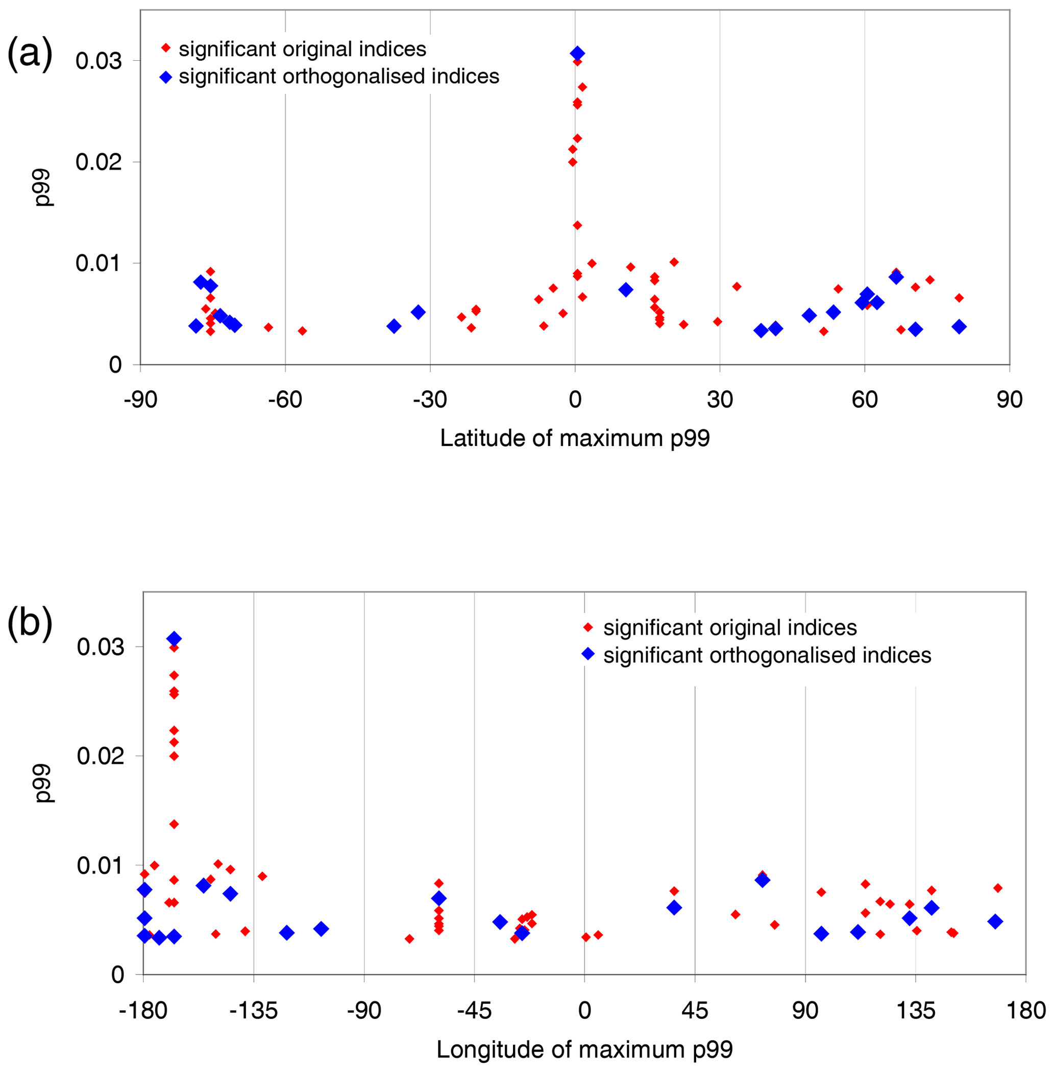
Figure 12Location of the 99th percentile of the delta rms values detected in the TCWV data derived from satellite observations as function of latitude (a) or longitude (b). Red points indicate results for the original indices, blue points for the orthogonalised indices.
Figure 12 shows the latitudinal (top) and longitudinal (bottom) distribution of the p99 values for all significant original indices (red) and all significant orthogonalised indices (blue) detected in the TCWV data from satellite observations. As expected, the highest values (related to ENSO) are found over the equatorial eastern Pacific, but most indices have the strongest effects in mid and high latitudes. Interestingly, in the latitude range between −30 and +30∘ only for one significant orthogonalised index (besides ENSO) the maximum delta rms is found. Another interesting finding is that several indices have their p99 values close to the date line (between 167 and −180∘ latitude). Four of these indices are also located at similar latitudes (between 38 and 71∘ N). In that region, also previous studies found enhanced activity (e.g. Hsu and Lin, 1992; Hoskins and Ambrizzi, 1993; Trenberth et al., 1998). One possible reason for the enhanced activity in this area might be the effect of jet exit regions, which are driven to a large extent by the Earth's topography (Feldstein and Franzke, 2017).
We investigated if and how strong the temporal patterns of a large set of teleconnection indices can be identified in the spatio-temporal variability of a global data set of the total column water vapour (TCWV) from 1995–2015 derived from satellite observations. To our knowledge, it is the first time that a global TCWV data set was used in such a detailed way in teleconnection studies (note that part of this data set was already used by van Malderen et al., 2018). Here it is important to note that the TCWV data set is purely based on observational data. Another important achievement of this study is the development of a new empirical method to decide whether a teleconnection index is significantly detected in the global data set. The method is based on temporally reversed teleconnection indices, which ensures that all relevant timescales are considered. The new method can be applied in a universal way to different data sets. In this study we applied the new method to the TCWV sets derived from satellite or model data as well to several further quantities, which are often used in teleconnection studies. Based on the obtained results, we could derive the following main conclusions related to the science questions mentioned in the introduction:
- a.
We developed a new empirical approach to determine whether a teleconnection index is significantly detected in a global data set. This approach avoids problems of existing algorithms for the determination of significance, because no assumptions on the significance level or the measurement uncertainties have to be made. We applied the new method to a global data set of the TCWV derived from satellite observations and found that 40 teleconnection indices could be significantly detected.
- b.
We applied the same method also to TCWV from the ERA interim data set. Here we used two versions of the model data sets: one including all data, the other only clear-sky data. The results for both versions agree in general very well with those for the satellite data set. This confirms both the quality of the satellite and model data sets. It also indicates that the satellite observations can be seen as representative of all day mean values. For some teleconnections, however, also systematic differences, mainly over northern Africa, were obtained. Since these differences are not found for the majority of the teleconnection indices, we conclude that they are very probably not related to systematic errors of the satellite data set, but rather they indicate shortcomings of the model over these regions.
- c.
We also applied our method to a variety of other data sets, which are usually used in teleconnection studies (surface temperature, surface pressure, geopotential heights and meridional winds at different altitudes). For most of these data sets fewer teleconnection indices were significantly detected than for the TCWV data sets, while for zonal winds, more teleconnection indices (up to > 50) were significantly detected. These results indicate that our global TCWV data set is well suited for teleconnection studies. In our view, this is an important aspect, because our data set is exclusively based on measurements. The strongest teleconnection signals were detected for the data sets of tropospheric geopotential heights and surface pressure. This finding is consistent with the fact that most teleconnection studies are based on these quantities. Another interesting finding is that in none of the global data sets, non-teleconnection indices (like the solar variability, the stratospheric AOD or the hurricane frequency) were significantly detected.
- d.
We investigated the spatial distribution of the teleconnection patterns. In particular we calculated global maps for the cumulative effect of all teleconnection patterns. For that purpose we first orthogonalised the teleconnection indices to avoid the effect of correlation between the indices. Compared to the original set of indices, much fewer of the orthogonalised indices (20 compared to 42) were significantly detected in the TCWV data set. Our global map of the cumulative effects of all significantly detected orthogonalised teleconnections showed the strongest teleconnection signals in the global TCWV data set over the tropics and in polar regions. These spatial patterns point to the importance of different driving mechanisms in different regions.
A1 Normalisation of the delta rms values
In many teleconnection studies (e.g. Horel, 1981, and references therein), the strength of a teleconnection index is quantified by calculating the ratio of the difference of the rms (with and without an index included) and the total rms. In this study we applied a different procedure, because the total rms depends on many factors, in particular also on the uncertainties of the considered data set. Since we want to compare the delta rms values derived for different data sets (in particular the TCWV data sets derived from satellite observations and model results, but also other data sets) in a quantitative way, we decided to divide the rms (with and without an index included) by the zonal mean of the considered data set. Thus the delta rms shows the relative impact of the respective index. While the rms values of the different TCWV data sets are rather different (see Fig. 4, middle panel), the zonal means are very similar (Fig. 2). The zonal mean was chosen (instead of the long-term average of each considered pixel), because for some data sets used in this study (especially the wind data sets) large variations and even zero-crossings exist, which would lead to meaningless delta-rms values. We compared the delta rms values calculated by our new definition with those of the more traditional definition for the TCWV data sets (Fig. A1). The obtained global patterns of both delta rms definitions are almost identical.
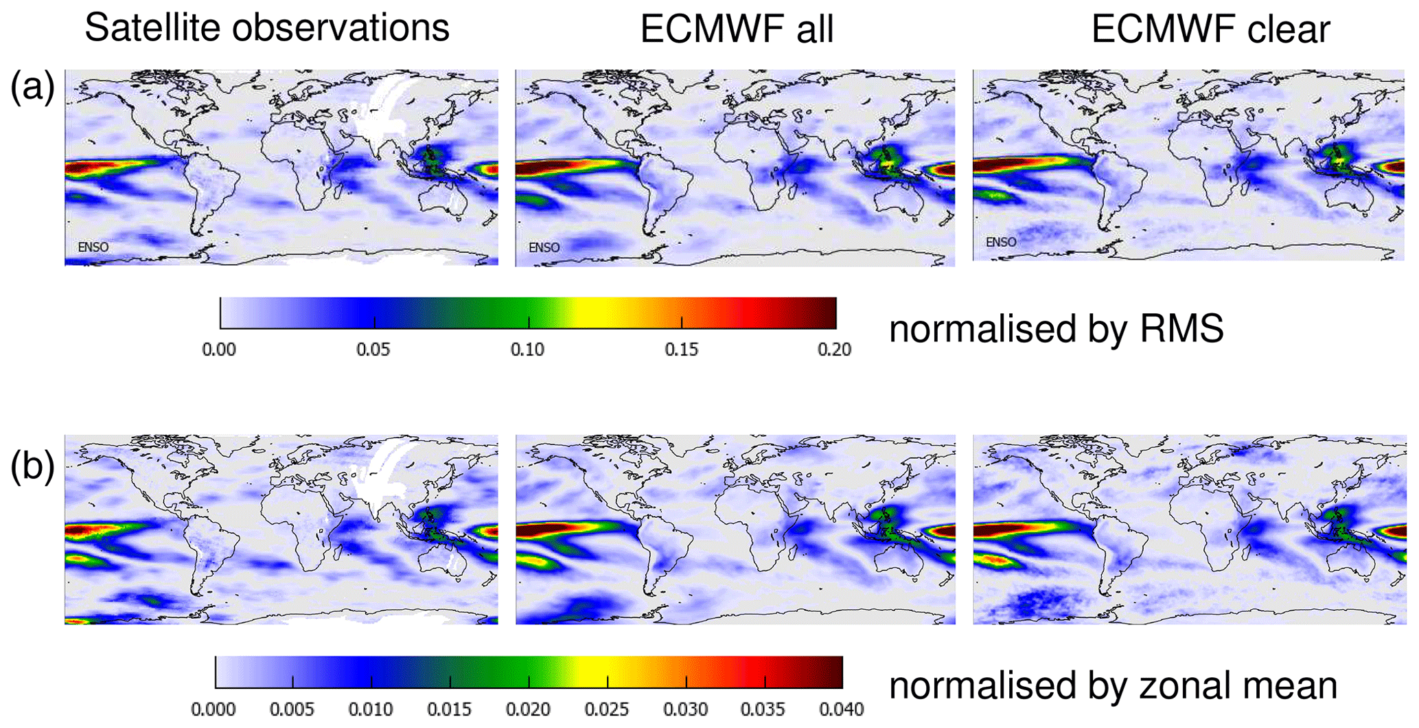
Figure A1Comparison of delta rms values for the ENSO index calculated in two different ways. (a) The difference of the rms with and without the ENSO index included in the fit is divided by the respective rms of each pixel; (b) the difference of the rms with and without the ENSO index included in the fit is divided by the zonal mean of the TCWV at the same latitude. Note the different colour scales.
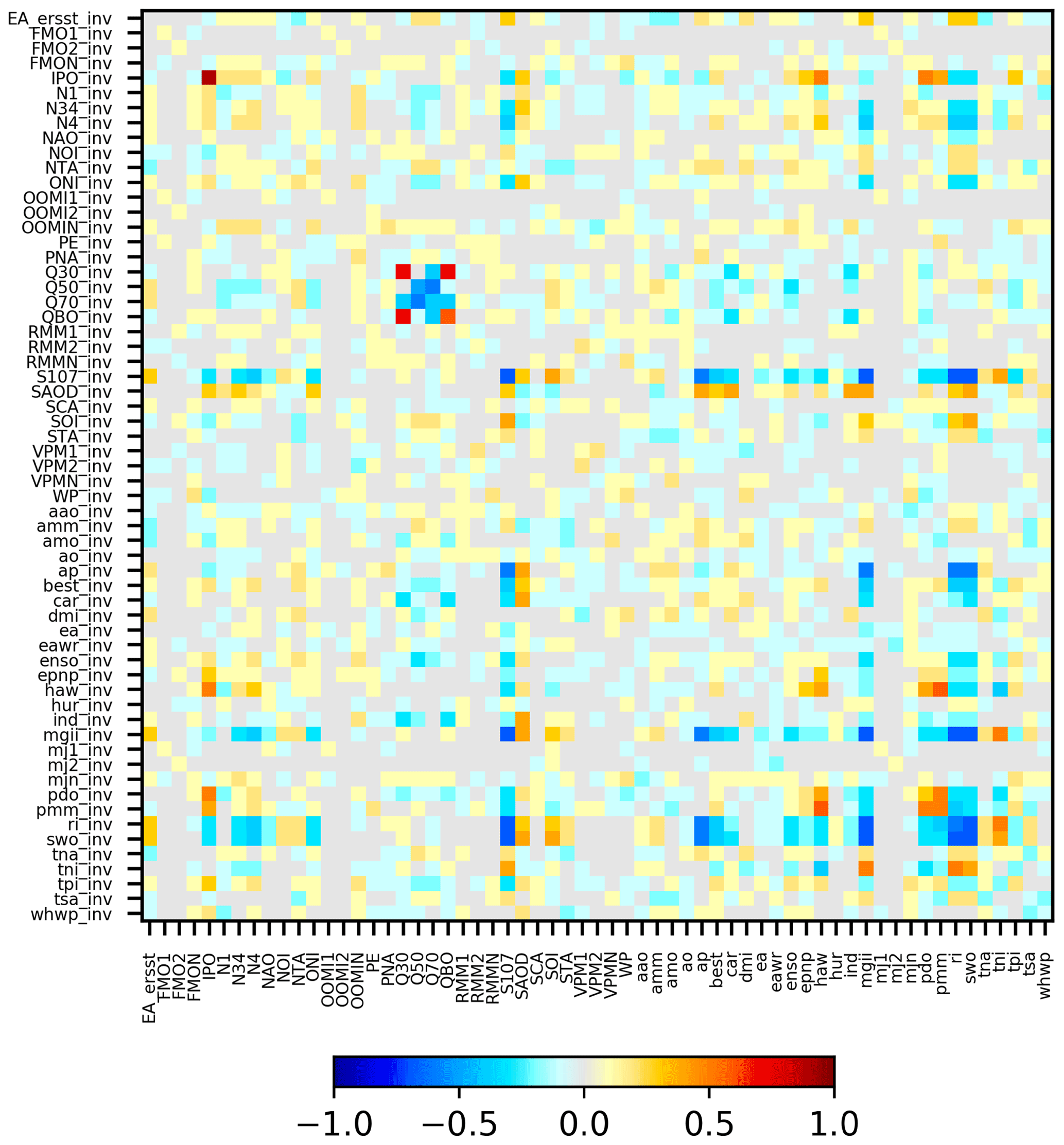
Figure A2Correlation coefficients between the temporally reversed and original indices. For several combinations enhanced coincidental correlations are found.
A2 Effect of the temporal correlation of the reversed indices with the original indices
For several temporally reversed indices, the 99th percentiles in Fig. 7 are substantially higher than for others. Since all reversed indices represent non-geophysical variations, such enhanced 99th percentiles are not expected. Thus this finding was further investigated. It turned out that the enhanced values are caused by accidental correlations of these reversed indices with original indices (see Fig. A2), for which high 99th percentile values are found. This reasoning is confirmed by the results shown in Fig. A3. There, high p99 values for reversed indices are always found if they are correlated with original indices with high p99 values. To avoid the effects of such accidental enhanced p99 values, only the reversed indices with no obvious correlations with original indices with high p99 values were kept for further processing (red boxes in Fig. A3). Here it should be noted that two somewhat arbitrary choices were made:
- a.
The selection of the selected reversed indices (red boxes in Fig. A3) was made by visual inspection.
- b.
The effect of the correlation of the reversed indices with the original indices was only investigated for the eight original indices with the highest p99 values.
Fortunately, both choices had only a minor influence on the derived threshold value. With respect to the first point, it should be noted that while the selection was made rather conservatively, still many reversed indices were kept after the filtering process. It was also found that most of the skipped reversed indices were removed because of enhanced correlations with several original indices. With respect to the second point it should be noted that it makes sense to consider only the original indices with the highest p99 values, because the correlations of the reversed indices with the original indices are in general rather low (see Fig. A2). The p99 values of the selected eight original indices with the highest p99 values are in general substantially higher than the p99 values of the remaining indices. In sensitivity studies we found that taking into account more than eight original indices had a negligible effect on the derived threshold values.
The red markers in Fig. A4 represent the p99 values for the indices which were kept after applying the selection criteria explained above. In the final step, from these p99 values the average and standard deviation are calculated. The p99 threshold for the significance of an index is then calculated as the sum of the average plus 3 times the standard deviation (for the TCWV data set from satellite observations the threshold is , including rounding). This procedure was chosen, because the threshold values calculated in this way are very close to the maximum p99 values of the remaining indices (red dots in Fig. A4) but are hardly affected by possible remaining outliers. The derived threshold value is indicated by the dashed black line in Fig. 7.

Figure A3Correlation plots for the eight original indices with the highest p99 values. The blue dots represent the 61 reversed indices. The x axis describes the correlation coefficients of the reversed indices with the selected original indices. The y axis describes the p99 value or the reversed indices. High p99 values are found for the reversed indices which show high correlation to the original indices.
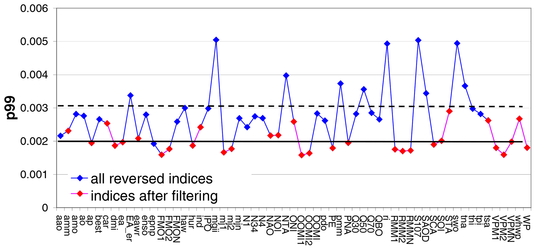
Figure A4The 99th percentiles (p99) of the delta rms of the temporally reversed indices for the TCWV from satellite observations (same as in Fig. 7, top). The blue markers indicate indices which are excluded from the calculation of the significance threshold (for details see text).

Figure A5Top: 99th percentiles (p99) of the delta rms values for the original (blue) and shifted indices (green: plus 1 month; red: minus 1 month). The indices are sorted from highest to lowest p99 values for the unshifted original indices. Bottom: ratios of the p99 values of the shifted and original indices. Results are for the TCWV data set from satellite observations. The blue circles indicate teleconnection indices with p99 values below the threshold, but ratios of the shifted indices < 0.8.
A3 Effect of a time shift of the teleconnection indices
In addition to the p99 values themselves, also the effect of time shifts month of the indices on the p99 values was considered to decide whether an index was significantly identified in a global data set, because for indices with a geophysical relationship to a considered data set, the exact temporal synchronisation should be important (but might depend on region). In contrast, for indices without a geophysical relationship to the considered data set, the p99 values should not depend on the exact temporal synchronisation. Here it should be noted that for some teleconnections, also time lags might exist between the corresponding indices and the atmospheric variables. Thus the lack of an exact synchronisation should not be seen as a strong indication that the corresponding teleconnection was not significantly detected in a global data set. But conversely, if a clear synchronisation for a teleconnection is found, this can be interpreted as a strong indication of significant detection.
In Fig. A5 the p99 values for the original and shifted (by ± 1 month) indices are shown for the TCWV data set from satellite observations. For most data sets (especially for those with high p99 values) indeed smaller p99 values are found for the shifted indices. Here it is interesting to note that in general a stronger effect is found for atmospheric indices than for oceanic indices, which can be understood by the higher frequencies of the atmospheric indices. For several oceanic indices, even higher values are found for the shifted indices indicating a time shift (mostly a time lag) between the TCWV and these indices. For one index (AMM) higher p99 values are even found for shifts in both directions indicating an ambiguity in the synchronisation between the TCWV and the AMM index.
Another interesting finding is that for some atmospheric indices with p99 values below the significance threshold (PE, MJ2, OOMI2, FMO1) still rather small ratios of the shifted and original indices are found indicating that these indices are also probably significantly detected in the TCWV data set. Thus in the following we consider also indices with p99 values below the significance threshold but with p99 ratios below 0.8 for both shifts as significantly detected. Here it should be noted that the choice of the threshold value of 0.8 is somewhat arbitrary. It was chosen because a deviation of 20 % from unity is larger than the “noise level” of the ratio. The exact choice of the threshold has only a small effect on the obtained results.
A4 Additional figures and tables

Figure A6List of original indices used in this study. Besides the short names also the data sources and their temporal variation from 1995 to 2016 are shown. ∗ All MJO indices are convoluted with a Gaussian kernel of 30 d FWHM. Original index according to Wheeler and Hendon (2004). Khaykin et al. (2017).
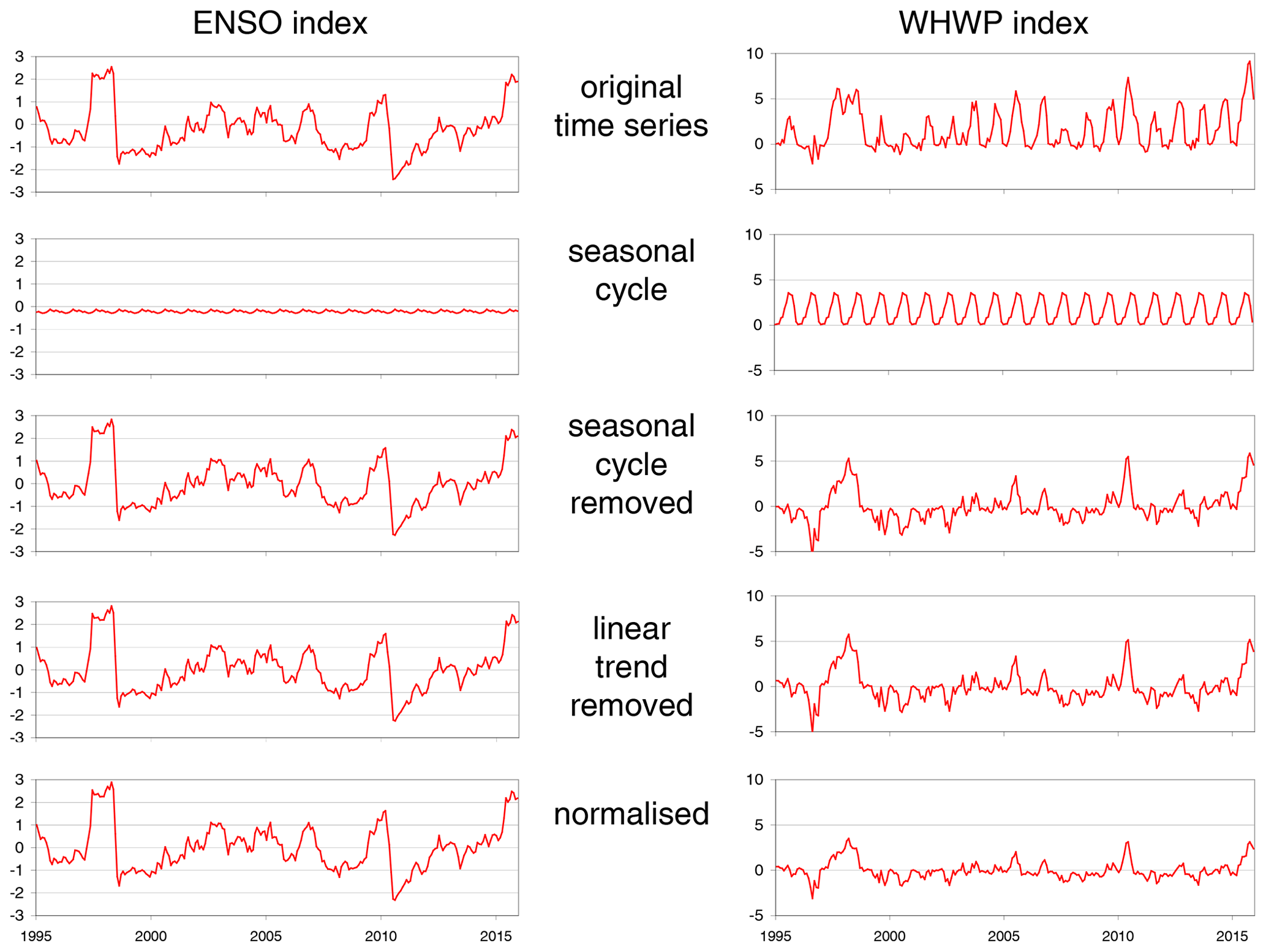
Figure A7Illustration of the preparations for the indices before they are used in the fit to the global data sets: first, the mean seasonal cycles and linear trends are subtracted. Then the differences are normalised by their standard deviations.
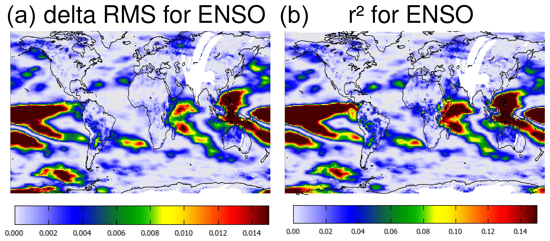
Figure A8Delta rms (a) and r2 values (b) for the fit of the ENSO index to the TCWV derived from satellite observations.
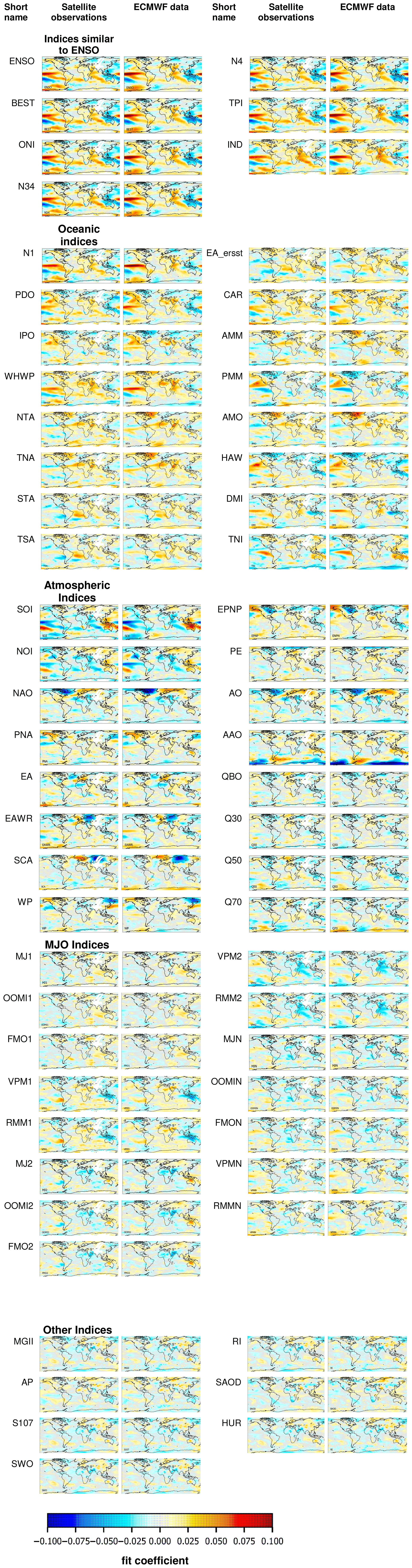
Figure A9Fit coefficients for all indices used in this study. Shown are the results for the TCWV data set from satellite observations (left) and model results (for all sky conditions) (right).
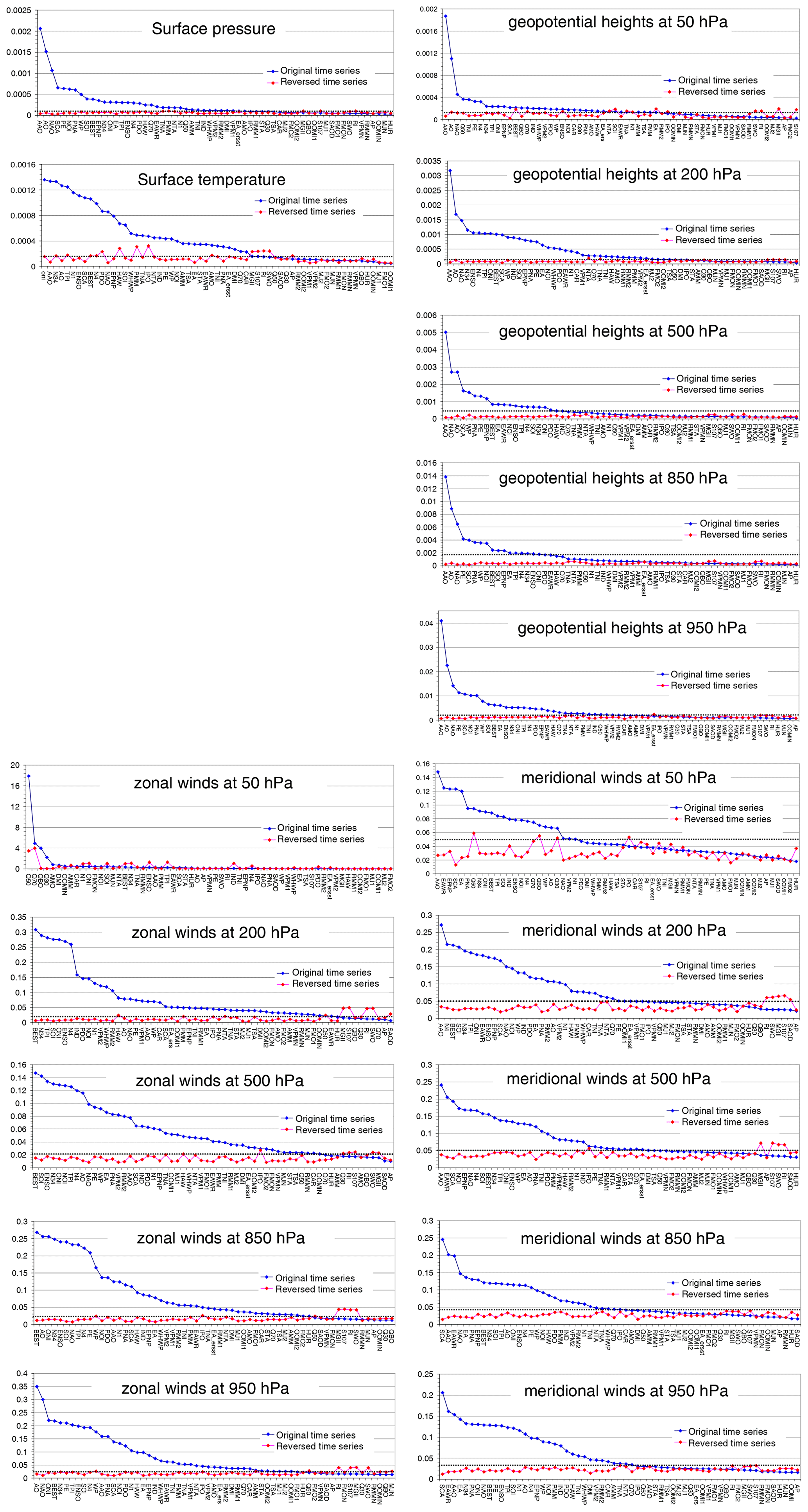
Figure A10The 99th percentiles of the delta rms values (p99) found for the different indices in different global data sets. Blue markers: p99 for the original indices; red markers: p99 for the temporally reversed indices; black lines: significance thresholds. The indices are sorted from highest to lowest p99 values for the original indices.
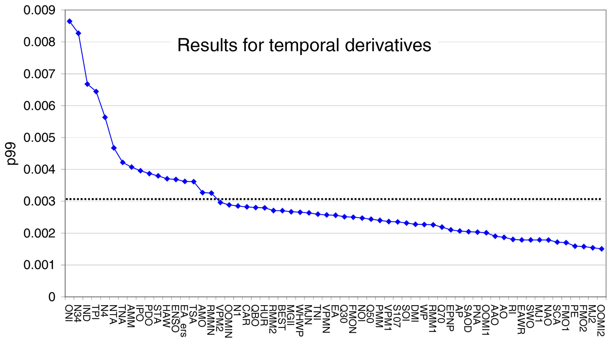
Figure A11The 99th percentiles (p99) of the delta rms of the derivatives of all indices. The black lines represent the significance threshold. The indices are sorted from highest to lowest p99 values.
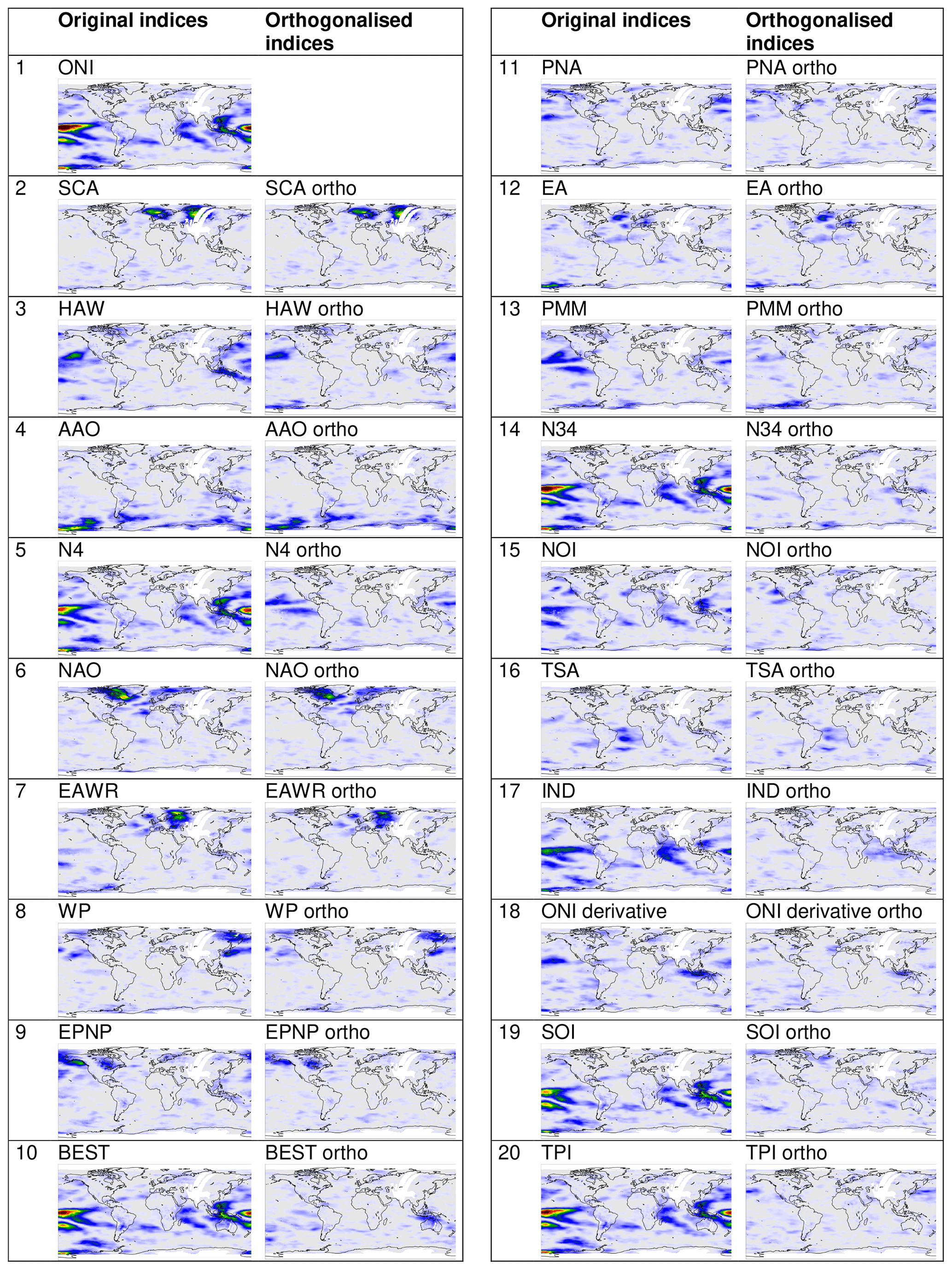
Figure A12Delta rms maps for the significant orthogonalised indices together with the delta rms maps for the original indices. The numbers at the left sides indicate the order (descending) of the p99 values (see also Fig. 10).
Table A1Significant indices for all data sets (indices with p99 values below threshold but shift ratios < 0.8 are indicated in brackets).
The TCWV data from satellite observations are available through Beirle et al. (2018). Other data sets are available from the authors on request.
TW initiated this study. TW and SB performed the data analysis. SD extracted the ECMWF data sets. TW, SB, SD, CB and RVM contributed to the interpretation of the results of this study.
Thomas Wagner is member of the AMT editorial board.
This article is part of the special issue “Analysis of atmospheric water vapour observations and their uncertainties for climate applications (ACP/AMT/ESSD/HESS inter-journal SI)”. It is not associated with a conference.
We want to thank the European Centre for Medium-Range Weather Forecasts (ECMWF) and many scientific and national institutions for making meteorological data and teleconnection indices available. We also thank ESA and EUMETSAT for making satellite spectra available. We are grateful to Holger Sihler for his valuable feedback and suggestions about the discussion of the significance derived from the fit.
The article processing charges for this open-
access publication were covered by the Max Planck Society.
This paper was edited by Marc von Hobe and reviewed by two anonymous referees.
Barnston, A. G. and Livezey, R. E.: Classification, seasonality and persistence of low frequency atmospheric circulation patterns, Mon. Weather Rev., 115, 1083–1126, 1987.
Beirle, S., Lampel, J., Wang, Y., Mies, K., Dörner, S., Grossi, M., Loyola, D., Dehn, A., Danielczok, A., Schröder, M., and Wagner, T.: The ESA GOME-Evolution “Climate” water vapor product: a homogenized time series of H2O columns from GOME, SCIAMACHY, and GOME-2, Earth Syst. Sci. Data, 10, 449–468, https://doi.org/10.5194/essd-10-449-2018, 2018.
Bjerknes, J.: A possible response of the atmospheric Hadley circulation to equatorial anomalies of ocean temperature, Tellus, 18, 820–829, 1966.
Bjerknes, J.: Atmospheric teleconnections from the equatorial Pacific, Mon. Weather Rev., 97, 163–172, 1969.
Danielczok, A. and Schröder, M.: GOME Evolution “Climate” product validation report, available at: https://earth.esa.int/documents/700255/1525725/GOME_EVL_L3_ValRep_final/db7e72c3-044d-4236-9dee-d88405b89ef0 (last access: 30 March 2021), 2017.
Dee, D. P., Uppala, S. M., Simmons, A. J., Berrisford, P., Poli, P., Kobayashi, S., Andrae, U., Balmaseda, M. A., Balsamo, G., Bauer, P., Bechtold, P., Beljaars, A. C. M., van de Berg, L., Bidlot, J., Bormann, N., Delsol, C., Dragani, R., Fuentes, M., Geer, A. J., Haimberger, L., Healy, S. B., Hersbach, H., Hólm, E. V., Isaksen, L., Kållberg, P., Köhler, M., Matricardi, M., McNally, A. P., Monge-Sanz, B. M., Morcrette, J.-J., Park, B.-K., Peubey, C., de Rosnay, P., Tavolato, C., Thépaut, J.-N., and Vitart, F.: The ERA-Interim reanalysis: configuration and performance of the data assimilation system, Q. J. Roy. Meteor. Soc., 137, 553–597, 2011.
Domeisen, D. I. V., Garfinkel, C. I., and Butler, A. H.: The Teleconnection of El Niño Southern Oscillation to the Stratosphere, Rev. Geophys., 57, 5–47, 2019.
Feldstein, S. B.: Teleconnections and ENSO: The timescale, power spectra, and climate noise properties, J. Climate, 13, 4430–4440, 2000.
Feldstein, S. B. and Frankze, C. L. E.: Atmospheric Teleconnection Patterns, in: Nonlinear and Stochastic Climate Dynamics, edited by: Franzke, C. L. E. and O'Kane, T. J., Cambridge University Press, Cambridge, UK, 54–104, 2017.
Horel, J. D.: A rotated principal component analysis of the interannual variability of the Northern Hemisphere 500 mb height field, Mon. Weather Rev., 109, 2080–2092, 1981.
Hoskins, B. J. and Ambrizzi, T.: Rossby Wave Propagation on a Realistic Longitudinally Varying Flow, J. Atmos. Sci., 50, 1661–1671, 1993.
Hsu, H. and Lin, S.: Global Teleconnections in the 250-mb Streamfunction Field during the Northern Hemisphere Winter, Mon. Weather Rev., 120, 1169–1190, 1992.
Hurrell, J. W.: Decadal trends in the North Atlantic Oscillation: regional temperatures and precipitation, Science, 269, 676–679, 1995.
Khaykin, S. M., Godin-Beekmann, S., Keckhut, P., Hauchecorne, A., Jumelet, J., Vernier, J.-P., Bourassa, A., Degenstein, D. A., Rieger, L. A., Bingen, C., Vanhellemont, F., Robert, C., DeLand, M., and Bhartia, P. K.: Variability and evolution of the midlatitude stratospheric aerosol budget from 22 years of ground-based lidar and satellite observations, Atmos. Chem. Phys., 17, 1829–1845, https://doi.org/10.5194/acp-17-1829-2017, 2017.
King, A. D., van Oldenborgh, G. J., and Karoly, D. J.: Climate change and El Nino increase likelihood of Indonesian heat and drought, B. Am. Meteorol. Soc., 97, 113–117, 2016.
Nigam, S. and Baxter, S.: General Circulation of the Atmosphere: Teleconnections, in: Encyclopedia of Atmospheric Sciences, edited by: Pyle, J. and Zhang, F., Elsevier Ltd., Amsterdam, 90–109, 2015.
Seabold, S. and Perktold, J.: Statsmodels: Econometric and Statistical Modeling with Python, in: Proceeding of the 9th Python in science conference (SCIPY 2010), 28 June–3 July 2010, Austin, Texas, 92–96, 2010.
Simpson, J. J., Berg, J. S., Koblinsky, C. J., Hufford, G. L., and Beckley, B.: The NVAP global water vapor data set: Independent crosscomparison and multiyear variability, Remote Sens. Environ., 76, 112–129, 2001.
Soden, B. J.: The sensitivity of the hydrological cycle to ENSO, J. Climate, 13, 538–549, 2000.
Thompson, D. W. J. and Wallace, J. M.: The Arctic Oscillation signature in the wintertime geopotential height temperature fields, Geophys. Res. Lett., 25, 1297–1300, 1998.
Trenberth, K. E., Branstator, G. W., Karoly, D., Kumar, A., Lau, N.-C., and Ropelewski, C.: Progress during TOGA in understanding and modeling global teleconnections associated with tropical sea surface temperatures, J. Geophys. Res., 103, 14291–14324, 1998.
Van Malderen, R., Pottiaux, E., Stankunavicius, G., Beirle, S., Wagner, T., Brenot, H., and Bruyninx, C.: Interpreting the time variability of world-wide GPS and GOME/SCIAMACHY integrated water vapour retrievals, using reanalyses as auxiliary tools, Atmos. Chem. Phys. Discuss. [preprint], https://doi.org/10.5194/acp-2018-1170, 2018.
Wagner, T., Beirle, S., Grzegorski, M., Sanghavi, S., and Platt, U.: El-Niño induced anomalies in global data sets of water vapour and cloud cover derived from GOME on ERS-2, J. Geophys. Res, 110, D15104, https://doi.org/10.1029/2005JD005972, 2005.
Walker, G. T. and Bliss, E. W.: World weather, V. Mem. Roy. Meteor. Soc., 4, 53–84, 1932.
Wallace, J. M. and Gutzler, D. S.: Teleconnections in the geopotential height field during the northern hemisphere winter, Mon. Weather Rev., 109, 784–812, 1981.
Wheeler, M. C. and Hendon, H. H.: An all-season real-time multivariate MJO index: Development of an index for monitoring and prediction, Mon. Weather Rev., 132, 1917–1932, 2004.
Wilks, D. S.: On “Field Significance” and the False Discovery Rate, J. Appl. Meteorol. Clim., 45, 1181–1189, 2006.
Wilks, D. S.: “The Stippling Shows Statistically Significant Grid Points”: How Research Results are Routinely Overstated and Overinterpreted, and What to Do about It, B. Am. Meteorol. Soc., 97, 2263–2273, 2016.
Woolings, T., Franzke, C., Hodson, D., Dong, B., Barnes, E., Raible, C., and Pinto, J.: Contrasting interannual and multidecadal NAO variability, Clim. Dynam., 45, 539–556, 2015.
Yeh, S.-W., Cai, W., Min, S.-K., McPhaden, M. J., Dommenget, D., Dewitte, B., Collins, M., Ashok, K., An, S.-I., Yim, B.-Y., and Kug, J.-S.: ENSO atmospheric teleconnections and their response to greenhouse gas forcing, Rev. Geophys., 56, 185–206, 2018.
- Abstract
- Introduction
- Data sets
- Teleconnection indices
- Analysis of global data sets
- Determination of significance
- Results for the different global data sets
- Orthogonalisation of indices
- Global distributions
- Conclusions
- Appendix A
- Data availability
- Author contributions
- Competing interests
- Special issue statement
- Acknowledgements
- Financial support
- Review statement
- References