the Creative Commons Attribution 4.0 License.
the Creative Commons Attribution 4.0 License.
 | 01 Apr 2021
Systematic detection of local CH4 anomalies by combining satellite measurements with high-resolution forecasts
Jérôme Barré
Ilse Aben
Anna Agustí-Panareda
Gianpaolo Balsamo
Nicolas Bousserez
Peter Dueben
Richard Engelen
Antje Inness
Alba Lorente
Joe McNorton
Vincent-Henri Peuch
Gabor Radnoti
Roberto Ribas
In this study, we present a novel monitoring methodology that combines satellite retrievals and forecasts to detect local CH4 concentration anomalies worldwide. These anomalies are caused by rapidly changing anthropogenic emissions that significantly contribute to the CH4 atmospheric budget and by biases in the satellite retrieval data. The method uses high-resolution (7 km × 7 km) retrievals of total column CH4 from the TROPOspheric Monitoring Instrument (TROPOMI) on board the Sentinel 5 Precursor satellite. Observations are combined with high-resolution CH4 forecasts (∼ 9 km) produced by the Copernicus Atmosphere Monitoring Service (CAMS) to provide departures (observations minus forecasts) at close to the satellite's native resolution at appropriate time. Investigating these departures is an effective way to link satellite measurements and emission inventory data in a quantitative manner. We perform filtering on the departures to remove the synoptic-scale and meso-alpha-scale biases in both forecasts and satellite observations. We then apply a simple classification scheme to the filtered departures to detect anomalies and plumes that are missing (e.g. pipeline or facility leaks), underreported or overreported (e.g. depleted drilling fields) in the CAMS emissions. The classification method also shows some limitations to detect emission anomalies only due to local satellite retrieval biases linked to albedo and scattering issues.
- Article
(5882 KB) - Full-text XML
- BibTeX
- EndNote


Atmospheric methane (CH4) is the second most important anthropogenic greenhouse gas after carbon dioxide; it contributes significantly to changes in radiative forcing and climate change. CH4 is estimated to account for at least a quarter of the present-day warming (Myhre et al., 2013) and has a near-term global warming potential that is 84 times larger than CO2 per unit mass (Hartmann et al., 2013). There are numerous natural and anthropogenic CH4 sources, which vary in location and areal extent. The related anthropogenic emissions, such as oil and gas production, coal mining and biomass burning, tend to be geographically localised, e.g. over a plant facility, a pipeline or a field of extraction. However, methane emissions relating to biological fluxes such as livestock, landfills and rice fields can be either geographically localised over narrow areas or more widespread; for example, there are extensive patterns of microbial respiration in wetlands across the globe (Saunois et al., 2016). Atmospheric methane concentrations have more than doubled since preindustrial times because of an imbalance between methane sources and sinks (Hartmann et al., 2013) caused by increases in oil and gas production, rice crop cultivation, livestock farming and landfills. Methane has a relatively short atmospheric lifetime (with respect to climate scales) of around 9 years, meaning that targeted emission reductions could be an effective way to limit the rate of warming over the coming decades (Shoemaker et al., 2013).
Greenhouse gas emission inventories are generated through the aggregation and extrapolation of regional and national data. These data are reported individually by countries using the guidelines provided by the United Nations Framework on Climate Change (UNFCC) and the Intergovernmental Panel for Climate Change (IPCC). The reporting follows a bottom-up approach that utilises activity data and emission factors from individual emissions sectors. The process of officially reporting and processing these data to build these bottom-up inventories can cause a significant lag, so information can be out of date for certain sectors once publicly released. This can become an issue in the context of rapidly changing emissions from large point sources, for example in the oil and gas sectors (Alvarez et al., 2018). In the case of atmospheric composition modelling, emissions inventories are used as input surface fluxes to simulate atmospheric concentrations. Within the Copernicus Atmosphere Monitoring Service (CAMS), these simulations are used to provide routine real-time forecasts of greenhouse gas concentrations. The CAMS greenhouse gas forecasting system integrates satellite observations (Massart et al., 2014, 2016) to generate initial conditions for high-resolution forecasts at about 10 km (Agustí-Panareda et al., 2019). The lack of up-to-date emissions inventories impacts and likely degrades simulated CH4 concentrations in areas where the local contribution from anthropogenic emissions is significant.
Many studies have demonstrated the rapidly changing and event-based nature of CH4 anthropogenic emissions, especially when identifying the locations of “super-emitter” point sources. Conley et al. (2016) used aircraft measurements to characterise a blowout of a well connected to the Aliso Canyon gas storage facility in California from October 2015 to February 2016. Pandey et al. (2019) showcased the detection of high methane emissions from a gas well blowout in Ohio during February to March 2018 using satellite measurements. More recently, Varon et al. (2019) detected an anomalously large CH4 source associated with a gas compression station using a combination of satellite instruments over Central Asia (western Turkmenistan). These types of suddenly occurring CH4 emissions cannot be or are not reported/detected in time to be included in the bottom-up inventories, but they are seen from space. Other studies have shown the ability of satellite measurements to detect CH4 emissions from extensive drilling and fracking areas. Kort et al. (2014) identified a large methane anomaly over the Four Corners region of the USA; more recently, de Gouw et al. (2020), Zhang et al. (2020) and Schneising et al. (2020) reported the satellite detection of large and extended CH4 enhancements from various US oil- and gas-producing regions, such as the Permian Basin. While these satellite-based studies focused on specific events and locations, none of them systematically detected such anomalies at a global scale; nor did they provide a method to do so.
The systematic detection of large point sources of anthropogenic CH4 emissions using a combination of satellite observations and modelling could prompt rapid action to reduce emissions from the oil and gas sectors. Two recent developments allow for the systematic detection of unreported CH4 atmospheric anomalies linked to small-scale and point-source emissions: the newly available high-resolution (7 km × 7 km) satellite observations from the TROPOspheric Monitoring Instrument (TROPOMI; Veefkind et al., 2012) on board the Sentinel-5P platform and the improved real-time forecasting at high resolution (∼ 9 km) provided by CAMS (Agustí-Panareda et al., 2019). In this paper, we present a novel methodology to routinely compare the satellite observations with the model forecasts in order to systematically detect atmospheric CH4 anomalies relating to emission changes from small-scale and point sources that are not reported or are not updated in a timely manner. The paper is organised as follows: Sect. 2 describes the setup, including the TROPOMI observations and the forecasting and monitoring configurations; Sect. 3 presents the detection method; and Sect. 4 discusses several case studies that showcase the capabilities but also the limitations of the detection method. This is followed by our conclusions, where we briefly discuss the benefit that our approach can bring combined with coarse-resolution inverse modelling.
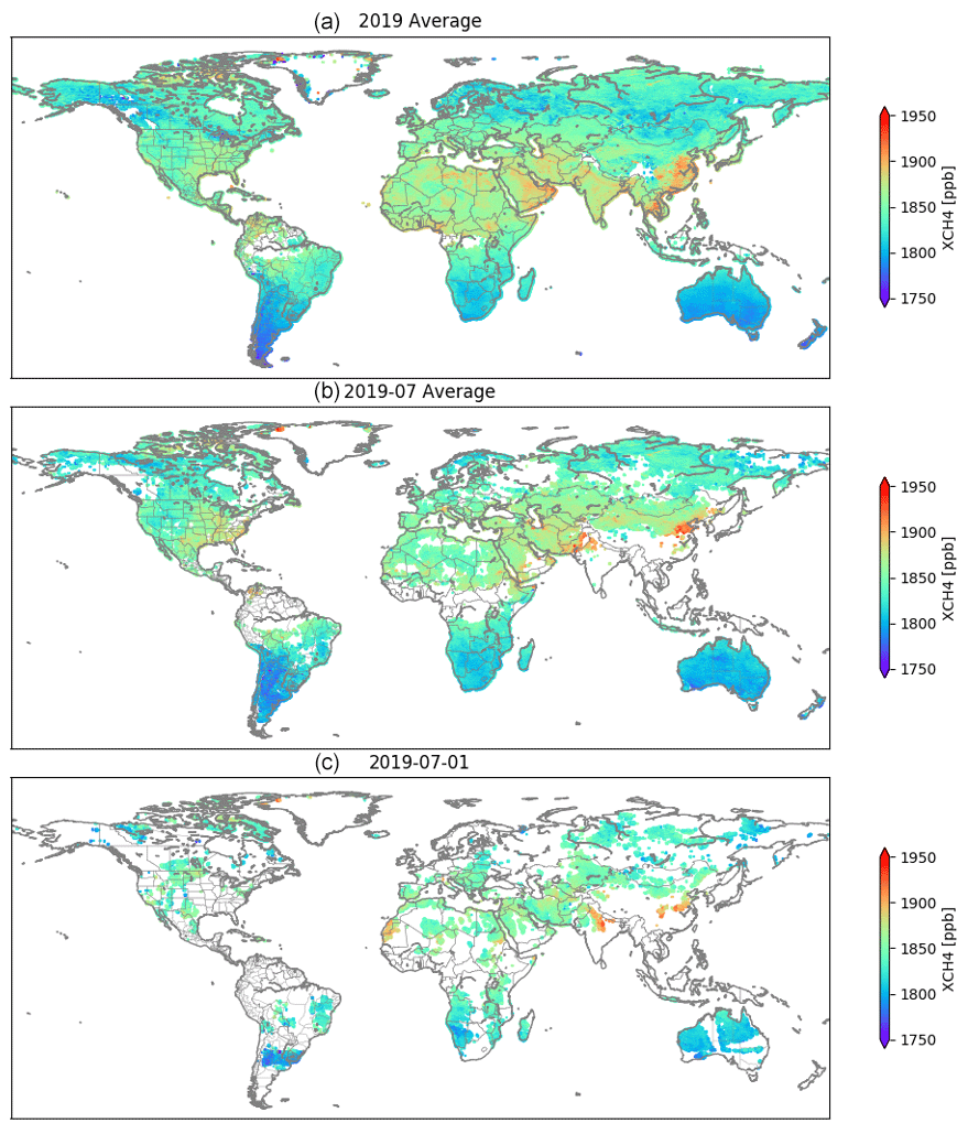
Figure 1Global average TROPOMI XCH4 column-averaged dry-air mixing ratios for the full year 2019, July 2019 and 1 July 2019 (a–c respectively).
2.1 TROPOMI CH4 observations
The TROPOMI (Veefkind et al., 2012) instrument was launched on 13 October 2017 on board the Sentinel-5 Precursor satellite, a low Earth orbiter with a Sun-synchronous orbit that overpasses at 13:30 local solar time. Operational since the end of April 2018, the instrument is an imaging spectrometer with a wide spectral range: ultraviolet, visible, near-infrared and shortwave infrared. This allows TROPOMI to measure a variety of atmospheric chemical species, such as ozone, nitrogen dioxide, carbon monoxide, sulfur dioxide, formaldehyde, aerosol and methane (Hu et al., 2018). Current CH4 observations, which are available for the inner two-thirds of the swath and only over land, are vertically integrated columns sensitive to the troposphere (surface to 200 hPa). With a swath that is around 1750 km (normally 2600 km) wide from the along-track position and a ground pixel size of 7 km × 7 km, TROPOMI CH4 data can provide near-global daily coverage at high horizontal resolution over land, but they are limited by cloud cover and retrieval quality. In this study, we use the bias-corrected version of the product and apply the most stringent quality flagging possible, selecting only pixels that have the qa_value = 1.0 (see Product Readme Methane V01.03.02, https://sentinel.esa.int/documents/247904/3541451/Sentinel-5P-Methane-Product-Readme-File, last access: January 2021). That document states that an overall bias of −0.3 % was found in a comparison against independent data, which is well within the mission requirements of ≤ 1.5 % (24 ppb). The scatter of the data around this bias also complies with the mission requirements of ≤ 1.0 % (18 ppb). Figure 1 illustrates the CH4 satellite observation coverage that TROPOMI provides per year, per month and per day.
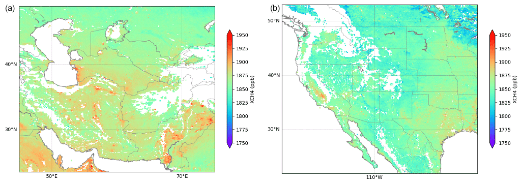
Figure 2Regional zooms of TROPOMI XCH4 columns for the full year 2019 in the Middle East (a) and central/western North America (b).
The measurements show clear geographical variation in the CH4 column-averaged dry-air mixing ratios (XCH4), which is driven to some extent by atmospheric transport but mostly by the spatial and temporal variability of surface fluxes and emission variations. Figure 2 shows the 2019 annual averages for the Middle East and the western USA. In these regions, spatial variability results in XCH4 enhancements of up to 50 ppb over emission hotspots. The average concentrations in these regions – approximately 1825 ppb over the USA and approximately 1875 ppb over the Middle East – are also significantly different. The strong local enhancements are an indication of strong local surface fluxes and emissions of CH4 from oil and gas activities, mining, agriculture or wetlands. XCH4 retrievals can also be prone to some systematic residual errors, especially those relating to surface albedo (Hasekamp et al., 2019). De Gouw et al. (2020), for instance, mentioned the possibility of retrieval biases due to low surface albedo in the shortwave-infrared spectral band during winter. Even though they are generally reduced in the bias-corrected product, such retrieval biases need further investigation (see Sect. 4.3). Nevertheless, the TROPOMI data are sufficiently accurate to show local enhancements linked (but not limited) to oil and gas production. We show in Sect. 3 how to isolate these small-scale signals of interest and remove the contribution of synoptic-scale (more than 2000 km) and meso-alpha-scale (between 2000 and 200 km) biases. In the rest of the paper, we define “large scale” as the combination of synoptic scale and meso-alpha scale.
2.2 CAMS high-resolution CH4 forecasting suite
In this study, we use the ECMWF Integrated Forecasting System (IFS), which is used in different configurations for the operational Numerical Weather Prediction (NWP) system as well as for the Copernicus Atmosphere Monitoring Service (CAMS) atmospheric composition analyses and forecasts. As part of the CAMS greenhouse gas services, the IFS provides 5 d forecasts for CO2 and CH4 (Agustí-Panareda et al., 2019) along with other species that are relevant to air quality (Flemming et al., 2015).
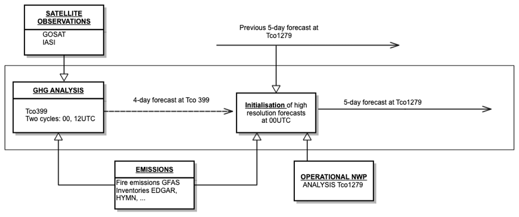
The IFS model cycle used in this paper is CY45R1. This is run routinely at TCo1279 horizontal resolution, which is a cubic octahedral reduced Gaussian grid at approximately 9 km resolution (Holm et al., 2016), 137 vertical levels from the surface to 0.01 hPa, and a time step of 450 s. Details about the transport and meteorological configuration can be found in Agustí-Panareda et al. (2019). The CAMS greenhouse gas (GHG) operational suite is composed of an analysis and forecasts at medium and high resolution (see Fig. 3). The analysis is based on the IFS 4D-Var assimilation system, which was adapted to assimilate retrieved column-averaged mole fractions of CO2 and CH4 together with all the operational meteorological observations (Engelen et al., 2009: Massart et al., 2014, 2016). The analyses are produced every 12 h (00:00 and 12:00 UTC). A 4 d forecast is then issued daily after the 00:00 UTC analysis on a TCo399 cubic octahedral grid corresponding to approximately 25 km × 25 km with the same 137-model-level configuration. Two satellite observation streams are currently assimilated: the Infrared Atmospheric Sounding Interferometer (IASI) for CH4 on the MetOp satellites and the Thermal And Near-infrared Sensor for carbon Observations (TANSO) on the GOSAT satellite for both CO2 and CH4 (see Massart et al., 2014, for further details). In this configuration, only the concentrations are corrected by the assimilation; the emissions and surface fluxes remain unchanged. Processing and acquisition of the level 2 data in 2019 yielded the satellite XCH4 data 4 d behind real time. The high-resolution forecast is then coupled to the analysis experiment by merging the 4 d lower-resolution forecast from the CO2 and CH4 analysis with the previous 1 d high-resolution forecast (Fig. 3) in order to preserve the fine-scale features of the high-resolution forecast. Additionally, the high-resolution forecast from the operational NWP runs is used to reset the initial meteorological conditions in order to ensure the best possible accuracy of the transport. In this paper, we will focus on using the CH4 forecasts at high resolution from the setup described above. The high-resolution forecasts are run on a TCo1279 L137 grid of approximately 9 km × 9 km for a 5 d period and are initialised approximately 4 h behind real time every day from 00:00 UTC. The impact of the TANSO and IASI CH4 retrieval assimilation is not strong close to the surface (see Fig. 8 in Massart et al., 2014). Analyses performed at a resolution of 25 km do not correct the emissions and hence mainly provide a correction to the forecast initial condition concentrations in the free troposphere and above. At lower altitudes, the emissions are the dominant influence on the 4 d forecast at 25 km, which is used to initialise the high-resolution forecast at 9 km that does not include data assimilation.
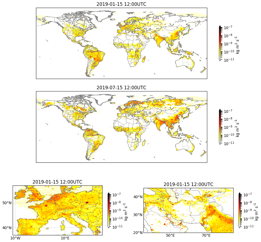
Figure 4Examples of combined net fluxes (only positive values are shown due to the logarithmic scale) that constitute the surface boundary conditions of the IFS high-resolution CH4 forecast. Global- and regional-scale examples for 15 January and 15 July 2019 at 12:00 UTC are presented.
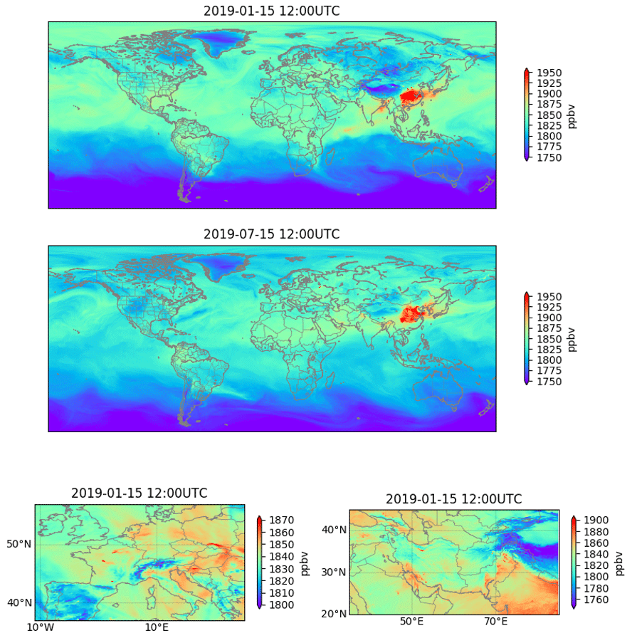
Figure 5Examples of the IFS high-resolution CH4 forecast output, showing snapshots at global and regional scales of the total column mean molar fractions for 15 January and 15 July 2019 at 12:00 UTC. The lower panels show parts of Europe (left) and the Middle East (right).
Both high-resolution forecasts and analysis use prescribed CH4 surface fluxes. The anthropogenic emissions data, including fossil fuel, agricultural and landfill/waste emissions, are from the EDGARv4.2FT2010 dataset (Olivier and Janssens-Maenhout, 2012) for 2010 with 0.1∘ × 0.1∘ and monthly resolution for the rice emissions (Matthews et al., 1991). Monthly mean wetland emissions come from a climatology (1990–2008) based on the LPJ-WHyMe model that is constrained by SCIAMACHY observations during the HYMN project (Spahni et al., 2011) and has a resolution of 1∘ × 1∘. The biomass burning emissions are from GFASv1.2 (Kaiser et al., 2012). Other sources and sinks include a monthly soil sink (Ridgwell et al., 1999), annual mean oceanic fluxes (Houweling et al., 1999; Lambert and Schmidt, 1993), and monthly mean fluxes from termites (Sanderson, 1996) and wild animals (Houweling et al., 1999). The chemical sink in the troposphere and stratosphere is represented by a climatological monthly mean chemical loss rate (Bergamaschi et al., 2009). This is based on OH fields optimised with methyl chloroform using the TM5 model (Krol et al., 2005) with prescribed concentrations of stratospheric radicals obtained using the 2D photochemical Max Planck Institute model. Figure 4 shows the geographical and seasonal structure of the surface fluxes. Large-scale and smoother structures are representative of wetland, soil and agricultural fluxes, whereas the finer-scale and sharper structures are representative of anthropogenic and fire emissions. Figure 5 shows the usefulness of the high-resolution forecasts at global and regional scales. Global seasonal cycles and synoptic-scale concentrations are represented, as well as concentrations at smaller scales, such as plumes from point-source emissions and orographic effects. Large point sources and associated plumes can be seen over Europe, for example over Madrid, Paris and Tours (western France). Inventory estimates suggest that the modelled hotspot region near Tours is probably the result of solid-waste landfill emissions. Other possibilities include emissions from the enteric fermentation and wastewater treatment sectors, all of which may be linked to a landfill site. Over the Middle East region zoom, sharp point sources are seen in Teheran and southern Iran, as well as over Pakistan (Karachi) and closer to the Himalayan region.
2.3 Monitoring suite
To monitor and compare the TROPOMI XCH4 retrievals with the IFS CH4 9 km forecasts, we reuse part of the IFS assimilation system in a so-called monitoring mode. The system recomputes a high-resolution trajectory at 9 km (which is a model integration), initialised from the forecasts in a 12 h monitoring window, to calculate so-called first-guess departures (a departure is the difference between an observation and the corresponding model forecast) using the observations at the appropriate model time step. At each observation location, the departure can be written
where d is the departure, y is the observation, H is the observation operator, M is the model integration or trajectory, and xi is the initial CH4 condition at the beginning of the monitoring window. If we inject the retrieval equation (Rodgers, 2000), the departure becomes
where xt is the true CH4 concentration state (which is never known exactly), A is the averaging kernel matrix (which represents the sensitivity of the retrieval on the vertical profile to the true state), I is the identity matrix, xa is the information known a priori that is used in the retrieval, and ϵ is the retrieval error term. The equation then simplifies to
which is the difference between the true state and the forecast smoothed by the averaging kernel function plus the retrieval error term. Those departure values are thus strongly dependent on the averaging kernel function shape. For the TROPOMI XCH4 retrievals, the mean averaging kernel function shows a homogeneous sensitivity to the entire troposphere, slightly decreasing in the stratosphere (see Fig. 2 in Hu et al., 2016). The averaging kernel function does not vary markedly between pixels or regions of the globe (not shown). Figure 6 shows the departures over various timescales (yearly, monthly and daily) for the global domain. Overall, the departures (observation minus forecast) show a global positive bias of around 25 ppb (meaning that the observation values are higher than the model values), which can be attributed to model biases (Ramonet et al., 2019) and/or observation biases (Langerock et al., 2019). Ramonet et al. (2019) compared the CAMS CH4 forecasts with independent total column data. Results showed that the forecasts continuously underestimated the CH4 total columns by 5–20 ppb. Langerock et al. (2019) showed that the average total column bias for the TROPOMI CH4 retrievals was −0.32 % (i.e. around −5 ppb) with respect to ground-based measurements.
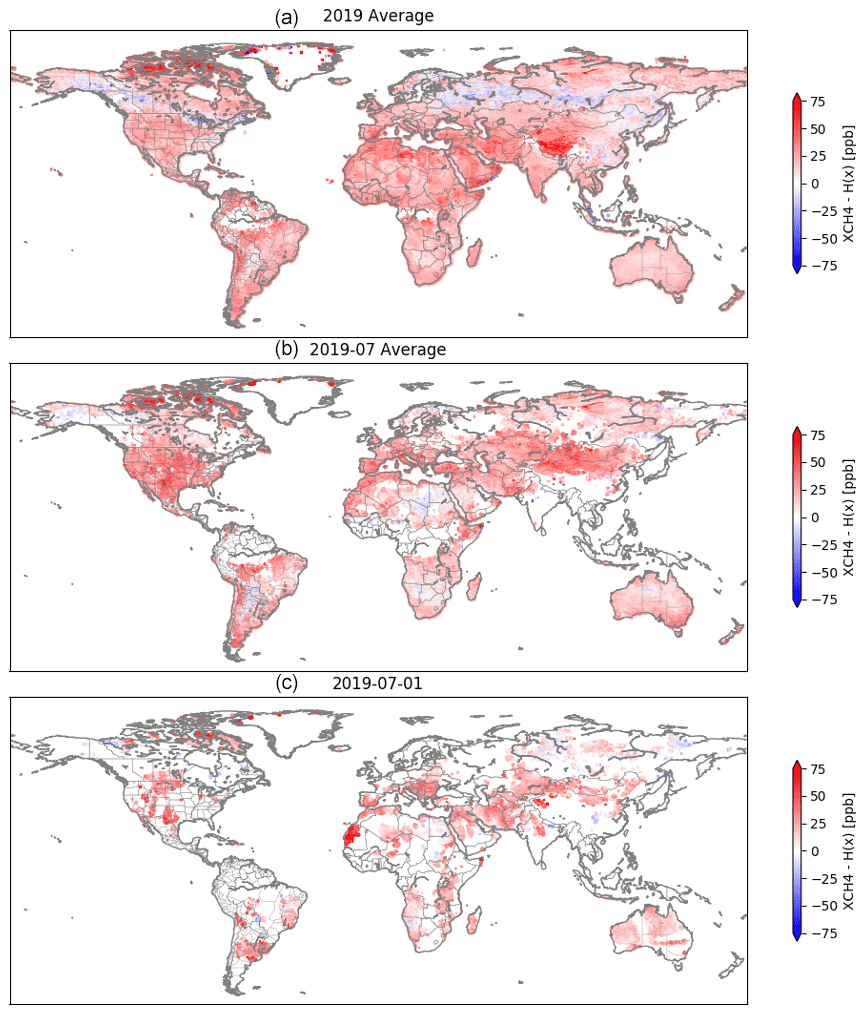
Figure 6Departure values computed with the observations displayed in Fig. 1 for the full year 2019, July 2019 and 1 July 2019.
Regional-scale error structures are evident from the observation–model comparison. For example, boreal regions show a band of negative values that are potentially attributable to systematic errors caused by surface albedo values during winter (see Sect. 2.1) in the TROPOMI retrieval algorithm. Alternatively, they could be caused by CH4 biases at the tropopause and lower stratosphere levels in the IFS model. Also, a possible time lag in the wetland emissions, which are calculated offline and provide boundary conditions in the IFS forecasting chain (see Sect. 2.2), could cause such errors. The origin of this type of large-scale error in the departures is not yet fully understood and is beyond the scope of this paper, although an understanding of these biases is crucial to further improving the quality of CAMS CH4 forecasts and TROPOMI retrievals. At finer scales, structures are seen on the yearly average comparison that become more evident at the monthly timescale. Local differences are even stronger at the daily timescale, but recognising fine-scale structures is challenging due to the lack of daily coverage. For these reasons, spatial filtering and temporal averaging of the departures are performed to extract and use the small-scale features seen in the departures.
3.1 Filtering the signal
To remove the large-scale features seen in the departures, we have implemented high-pass Gaussian filtering. The filter uses a convolution of a 2D Gaussian kernel on a given averaged and binned departure field. In this study, we use 0.1∘ latitude–longitude binning. Due to the ocean, cloud cover and quality control flagging, a number of departure bins will have missing values, which will jeopardise the convolution. This problem is solved technically by creating two auxiliary matrices in which missing values are replaced by 0. The two auxiliary matrices are then defined as
where dm (the subscript m refers to “mean”) is the average departure in the given bin and N is the minimum number of observations that must be included in a given bin. In this study, we use N=2 to avoid smoothing with very isolated (and potentially faulty) pixels while retaining as much data as possible. Replacing the missing values in D with zeros introduces an error in the filtered departures dhp (where the subscript hp refers to “high pass”) after convolution (lower values are induced by the smoothing resulting from the insertion of zeros). This can be corrected for by applying the same Gaussian filter to a matrix C representing the bins selected for filtering (where the number of counts is at least N) and using the ratio of the two filtered matrices to compensate for the missing-value errors. A high-pass filter on a given observation space field (departures here) can then be formulated as follows:
where G(σ) is a 2D Gaussian kernel function with a σ length scale. The same filtering is also applied to the observation values y and the first-guess values HM(xb), as these will be used for classification in Sect. 3.2. Figure 7 shows the effect of the filtering on the observation-space data using a 30 d window and a length scale of 2∘. Firstly, we can see that the large-scale features in the departures such as the overall bias and regional variations are removed. Secondly, the departure, observation and first-guess distributions are made more Gaussian, such that the distributions is centred at zero and is more symmetrical, and display tails. This makes the processing and classification of the data much easier (see Sect. 3.2).
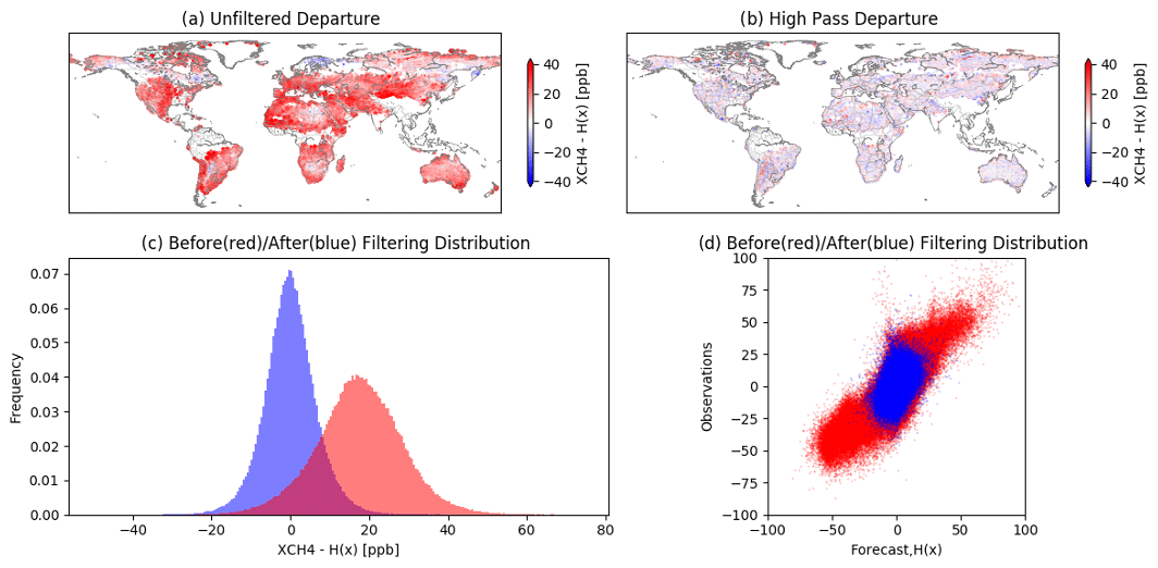
Figure 7Example of the effect of high-pass filtering on observation-space data using a 30 d window ending on 1 July 2019 with a 2∘ Gaussian kernel length scale: (a) the unfiltered departures, (b) the filtered departures, (c) histograms comparing unfiltered (red) vs. filtered (blue) departures, and (d) 2D distributions of the unfiltered (red) and filtered (blue) data points in the observation–forecast space. Note that the unfiltered data distribution is centred at the mean in this plot to facilitate comparisons with the filtered distribution.
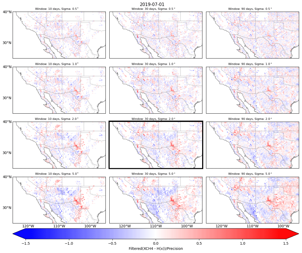
Figure 8High-pass filtering sensitivity tests of the departures normalised to the instrument precision. Window length (columns) is 10, 30 or 90 d, and kernel size (rows) is 0.5, 1.0, 2.0 or 5.0∘. The selected filter parameter values are those for the plot outlined in bold.
To decide on the appropriate window length and Gaussian kernel length scale, we conducted sensitivity tests with different length scales (σ = [0.5, 1.0, 2.0, 5.0]∘) and window lengths of 10, 30 and 90 d. Figure 8 shows the resulting filtered departures normalised to the instrument precision for the 12 possible sensitivity tests. For the tests with Gaussian kernel sizes of 0.5 and 1.0∘, the filtered signal is generally weaker than the measurement precision, so very few or no detections of local anomalies will be made. Conversely, if the kernel is large, the signal is stronger relative to the instrument precision, but there is a risk of picking up larger patterns than the targeted features, i.e. features that are directly related to local emissions in the atmospheric distribution of CH4. For these reasons, we found that a kernel of 2.0∘ performed best. If the time window is short, e.g. 10 d, decreased coverage could hinder the correct detection of outliers, especially for isolated data points. Isolated data points that indicate possible outliers could be filtered out towards 0, as the convolution does not have neighbouring points to use within the kernel range. The shorter the window and the narrower the kernel, the more likely this is. Conversely, using a long time window, i.e. 90 d, maximises the chances of achieving good observation coverage, allowing the most effective use of the convolution filter, although this reduces the ability to provide information on temporal variability. Also, the sharp spatial structures that correspond to more recent or sporadic emission events are smoothed by the time averaging, decreasing the filtered departure over instrument precision ratio. For these reasons, we found that a time window of 30 d provides the most reasonable results.
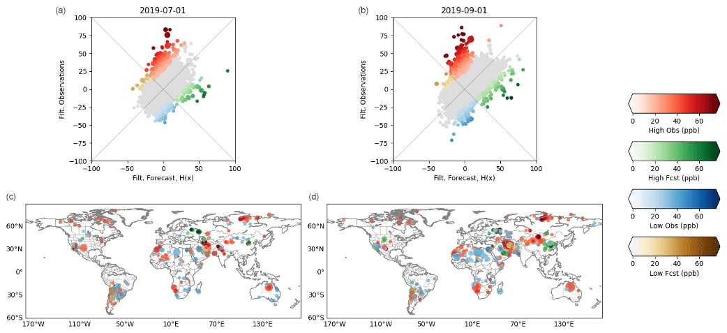
Figure 9Examples of outlier classification. (a, b) Global distributions in the observation–first-guess space for two different 30 d windows (end dates: 1 July and 1 September 2019). The four data classes are shown in different colours; the colour intensity reflects the number of outliers. (c, d) Locations of outlier classes around the globe during the two 30 d windows (end dates: 1 July and 1 September 2019, respectively). Darker dots show larger departures. Larger dots indicate that more occurrences were detected in the bin and time window.
3.2 Outlier classification
The final step is outlier detection of the filtered departures. We choose to retain the filtered departures with absolute values that are larger than the CH4 measurement precision of TROPOMI. If the absolute value of a filtered departure is lower than the measurement precision, it is considered noise and ruled out. The current methodology could be refined to find a better outlier detection method based on more advanced statistical techniques. In the present study, we found that the measurement precision of the satellite product provides suitable results. In addition to outlier detection, we classify the departures into four categories based on the relative values and signs of the filtered observations and forecast values:
-
High observations (red in Fig. 9), where the filtered observation values are higher than the absolute filtered forecast values. This class represents XCH4 values that are high according to TROPOMI but are not seen as high or not seen at all in the forecasts. These likely originate from emissions that are not reported or are underestimated in the inventories. However, high observations may also be caused by poor-quality observations due to albedo and scattering issues (see Sect. 4.3).
-
High forecasts (green in Fig. 9), where the filtered forecast values are higher than the absolute filtered observation values. This class represents CH4 values that are high in the forecasts but are not seen as strong or not seen at all in the TROPOMI XCH4 retrievals. High forecasts likely originate from emissions that are overestimated, no longer being produced, or even mislocated in the emissions inventory.
-
Low observations (blue in Fig. 9), where the filtered observation values are lower than the absolute filtered forecast values. This class represents XCH4 values that are locally low according to TROPOMI but are not seen to be as low or are not seen at all in the forecasts. Poor-quality observations that are influenced by low surface albedo likely fall in this category (see Sect. 4.3).
-
Low forecasts (gold in Fig. 9), where the filtered forecast values are lower than the absolute filtered observation values. This class represents XCH4 values that are low in the forecasts but are not seen to be as low or are not seen at all in the TROPOMI XCH4 retrievals. This category generally includes relatively few data points, which are very sparsely distributed. Orography may explain the data points in this category (i.e. model surface heights that are higher than the corresponding observation values). Further improvements to our method will likely involve the use of orography to improve the filtering.
In the maps shown in Fig. 9, colour intensity indicates the magnitude of the offset, i.e. how far the observation value is from the forecast value. Point size indicates the number of samples included: a larger dot indicates that more data points within the 30 d window were used to compute the statistics, making them more robust. Figure 9 gives an overview of outliers detected around the world, which are many and varied. In the next section, we focus on specific case studies from the underreported/missed plumes (red) category and the overreported plumes (green) category to demonstrate both the usefulness of the method and its current limitations.
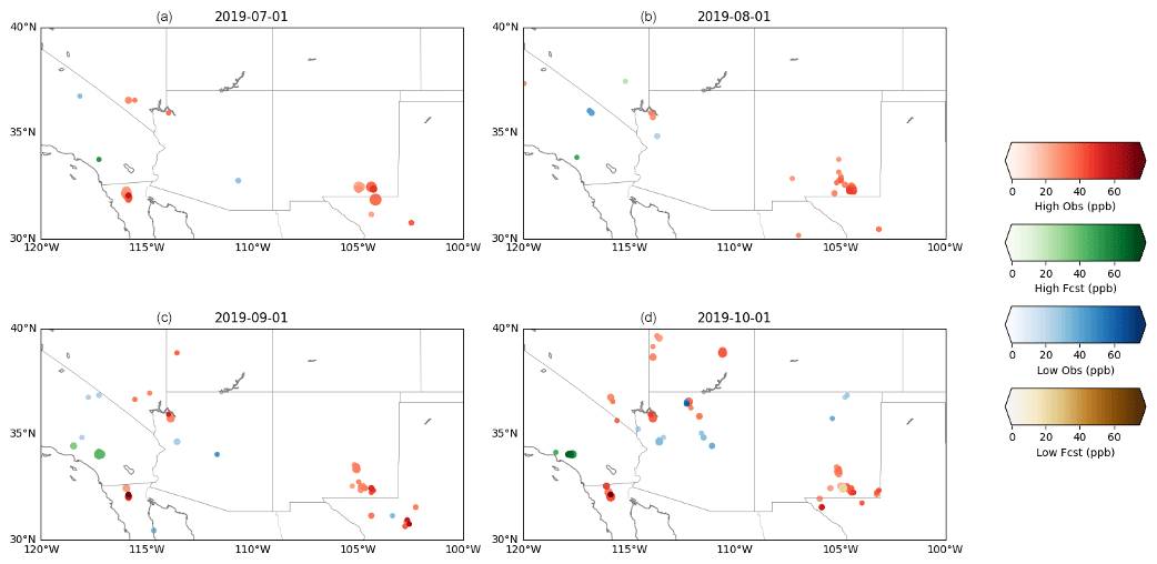
Figure 10Outlier detection and classification over the southwestern USA. Dates indicate the end date of the 30 d time window.
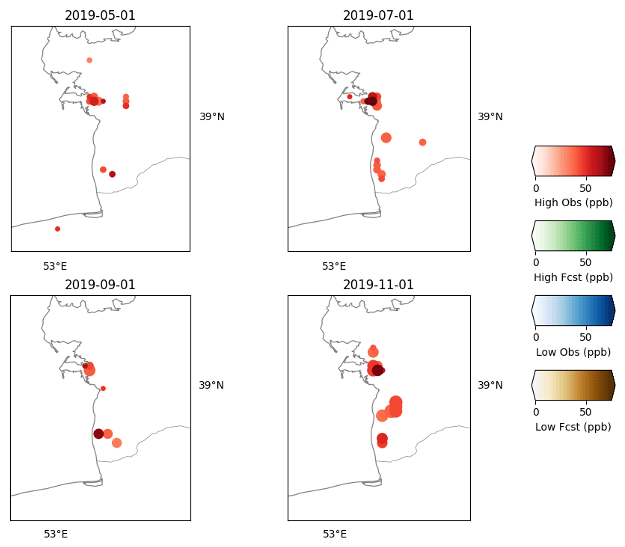
Figure 11Outlier detection and classification over Turkmenistan. Dates indicate the end date of the 30 d time window.
4.1 Underestimation of emissions from local sources in the forecasts
Southwestern USA and Mexico. Figure 10 shows that the method detects underpredicted local CH4 concentrations (in red) in the forecast system for three areas of the southwestern USA and Mexico. One area is in the Permian Basin, around the Texas–New Mexico border, where multiple oil drilling sites are currently operating. These enhancements have been documented by de Gouw et al. (2020) and Zhang et al. (2020), showing the reliability of the presented method. The two other regions have smaller biases and extents, and they occur around the southern tip of Nevada (by Lake Mead) and northern Baja California (close to the USA–Mexico border). To our knowledge, these two cases are yet to be investigated or documented, so they need further investigation. We could not identify any facilities that are responsible for those enhancements; neither could we find any matching land surface albedo features that could create local biases in the retrievals (see Sect. 4.3) from visible satellite imagery. The northern Baja California enhancements are observed to be correlated with scattering parameters such as the aerosol optical thickness (AOT, not shown), which should be investigated further to improve the method. A case study of the influence of the AOT on the detection method is described in Sect. 4.3.
Western Turkmenistan. To confirm the ability of this methodology to detect large point-source emitters, we also showcase the very strong detection of anomalous concentrations over western Turkmenistan. Strong enhancement occurred throughout 2019 (Fig. 11), although the enhancement changed in intensity and shape. The filtered departures can be very large (above 50 ppb), with high counts in the bins (i.e. large dots). As mentioned above, anomalously large CH4 sources linked to oil and gas production in this location have been documented and detected by Varon et al. (2019) using TROPOMI in combination with private-sector satellite data.

Figure 12Outlier detection and classification over western Russia. Dates indicate the end date of the 30 d time window.
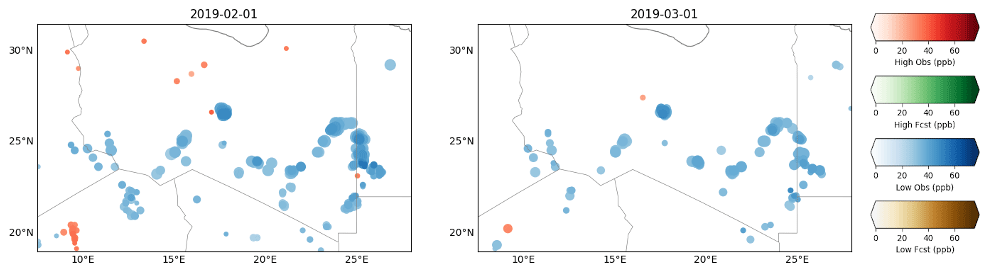
Figure 13Outlier detection and classification over Libya, Egypt and Niger. Dates indicate the end date of the 30 d time window.
4.2 Overestimation of emissions from local sources in the forecasts
Western Russia. Our detection system shows two local point sources with large forecast values that are not seen by TROPOMI XCH4 (green dots in Fig. 12). The features are depicted as small dots (i.e. relatively few samples) that form a plume shape, with strong departures near the point sources. One is very close to Moscow and corresponds to the surroundings of Domodedovo Airport. The other source is near the Volga River; its location correlates with small drilling fields seen in visible satellite images. The detection method suggests that emission inventories are overestimating emissions from these sources, which were actually releasing lower emissions or were no longer active emitters during the monitoring period.
Los Angeles. Similar features can occur in the area of Los Angeles. Figure 10 shows significant overprediction of CH4 (green dots) over San Bernardino and Palmdale. Both towns have industrial facilities and regional airports. Stronger detection is seen in the 1 September and 1 October 2019 windows than in the 1 July and 1 August 2019 windows. Differences in intensity may be attributed to changes in emission levels from month to month, as well as seasonal atmospheric transport changes due to different meteorological situations in different windows. For example, if the overall wind speed increases near the source, less accumulation of CH4 would be seen, leading to smaller departures and less detection.
Such cases in very different locations show the ability of the method to detect not only missing or underreported point sources but also overreported cases. This can only be achieved by combining numerical model forecasts and satellite measurements that have closely matched high horizontal resolutions (9 and 7 km respectively). It is also important to mention that the method presented here is subject to uncertainties due to model transport error and representation error, although the error associated with emission levels generally dominates. Further work is needed to account for atmospheric transport and, more generally, weather variability in the detection method. Techniques such as those described in Barré et al. (2020) show great potential for application in this context.

Figure 14(a, b) TROPOMI albedo in the near-infrared (NIR) band, (c, d) TROPOMI albedo in the shortwave-infrared (SWIR) band, and (e, f) TROPOMI XCH4 columns. Maps display averages for the same windows as shown in Fig. 13.
4.3 Local retrieval issues
The TROPOMI XCH4 retrieval can be affected by albedo issues (see Sect. 2), and the filtering is not able to remove features with geographical extents that are smaller than the size of the Gaussian kernel (see Sect. 3.1). Figure 13 shows patterns in the outlier detections where the filtered observations are lower than the filtered forecasts (low observation category; plotted in blue). Similar patterns are seen for the two months considered. In Fig. 14, the TROPOMI albedo in the near-infrared (NIR) and shortwave-infrared (SWIR) bands is displayed along with the XCH4 column retrieval. There are large albedo variations in the two spectral bands in this area that affect the XCH4 columns. The patterns for the albedo and the XCH4 columns clearly match. The ability of the filtering algorithm to remove this effect depends on the structure of the pattern and how narrow or small it is. This is an issue with the outlier detection method in its current form.
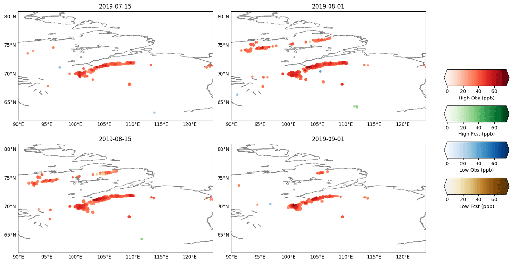
Figure 15Outlier detection and classification over Siberia. Dates indicate the end date of the 30 d time window.
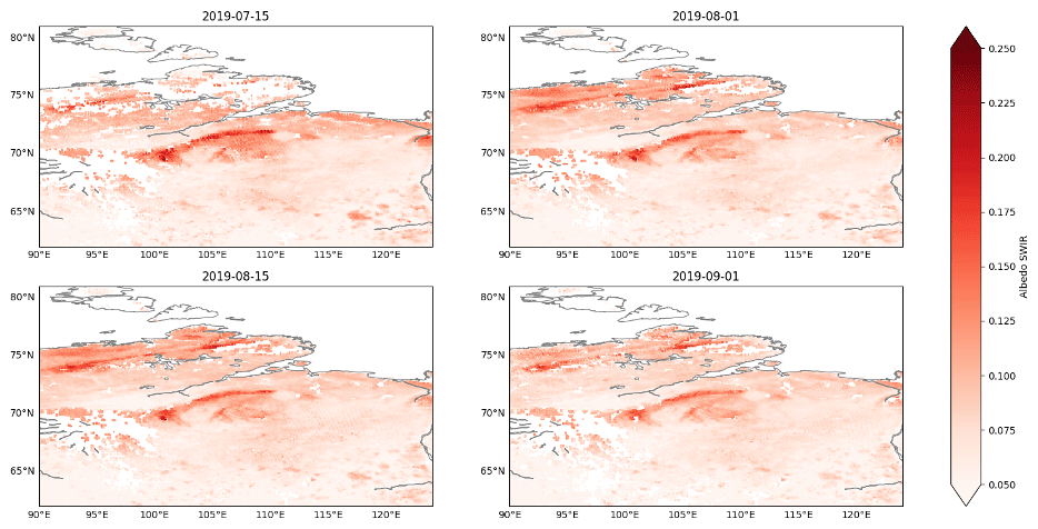
Figure 16Albedo in the shortwave-infrared (SWIR) band over Siberia, as provided by TROPOMI. Maps display averages for the same windows as shown in Fig. 13.
Another example is provided in Fig. 15, where the same pattern is seen repeatedly in the outlier detection over the Siberian region. In this case, the filtered observation values are higher than the filtered forecast values (high observation category; plotted in red). The pattern detected matches the SWIR albedo pattern shown in Fig. 16. The high-albedo areas in the SWIR albedo map are also the areas with relatively high TROPOMI XCH4 compared to their surroundings, and the pattern is narrow enough to be missed by the filter. Thus, great care should be taken when diagnosing such filtered departures. Features with a consistent distinctive shape and intensity are potential retrieval error artefacts, as atmospheric methane signals generally show considerable variability as a result of meteorological dynamics, not a consistently distinctive shape over a period of months (8 and 10 weeks in Figs. 13 and 15 respectively). Further development of our detection method should include the incorporation of albedo information to try to account for such systematic local biases.

Figure 17Outlier detection and classification over Australia. Dates indicate the end date of the 30 d time window.

Figure 18Aerosol optical thickness (AOT) in the near-infrared (NIR) band over Australia, as provided by TROPOMI. Maps display averages for the same windows as shown in Fig. 15.
However, in certain cases, identifying such biases can be more complex than just correcting outlier detections using albedo information. In Fig. 17, the anomaly presents a consistent shape for the four months shown when using 30 d windows, but there is no feature in the corresponding NIR and SWIR albedo maps that is clearly correlated with the anomaly. Instead, investigations showed that this anomaly is associated with scattering parameters such as the aerosol optical thickness (AOT); it correlates well with the AOT in the NIR and SWIR bands. As an example, Fig. 18 shows the presence of a feature in the map of the AOT in the NIR band that correlates to high-XCH4 observations with respect to the forecasts. A similar feature is also seen in the map of the AOT in the SWIR band (not shown). This shows that more work is needed to identify systematic local biases, as they are not all caused by albedo variations. Additionally, there is still a potential impact of temporally and spatially variable small-scale albedo features. For example, nonpersistent biases can arise with snow coverage. More research will be needed to improve automatic local bias detection for less persistent biases.
Currently, the method presented here helps to identify retrieval biases, but it does not do this systematically. Further improvements to the method could include the joint use of albedo and scattering parameters to perform additional filtering correction and flagging. The availability of such an automatic retrieval bias detection tool would help to improve the quality of the retrieval product.
In this paper, we have shown the potential for the systematic detection of anthropogenic CH4 point and local source emissions relative to known emissions inventory data using TROPOMI satellite measurements in combination with high-resolution CH4 forecasts. While many studies have included detailed analyses of a few case studies using TROPOMI observations, this is the first step towards providing a systematic way to detect strong local anthropogenic emitters of CH4 and to compare the results with emissions inventories. The method presented here not only shows the potential for the detection of unreported or missing sources, but it also targets overreported sources in the inventories. It also has the potential to identify systematic local retrieval errors, which could help to improve the satellite product. However, the current method has some limitations, as it requires additional correlative analyses with albedo and scattering parameters to account for local biases in the retrieval values. Complications can arise if land-surface-induced biases and detected local emission features are collocated. The presence of multiple types of collocated emissions (i.e. anthropogenic plus wetland emissions) will also increase the complexity, as emission patterns could show albedo correlations in this case. We have, however, demonstrated the potential of the methodology by focusing on several case studies, and further work is required to provide a global assessment based on several years from this dataset.
Our method is novel in that it combines information from multiple sources (emissions inventories, modelled surface fluxes and observations) in a data assimilation framework in order to detect and analyse observed anomalies. We used the global emissions inventories and fluxes that were the best possible global estimates available to us when we were running our system. Using other emissions inventories from research activities that are more specific to local regions could provide different answers. In this way, our methodology could provide an efficient way to validate improvements in sector-specific emission inventories. For example, using revised CH4 inventories such as those presented by Maasakers et al. (2016) for the USA or more recently by Scrapelli et al. (2020) for the entire globe could lead to different detection patterns. Bottom-up inventories will always lag in time and therefore cannot track rapid emission changes such as pipeline and gas facility blowouts. Satellite measurements have clear added value given that they can provide timely detection of large emissions.
Combining satellite measurements, forecasts and emissions inventories using a data assimilation system paves the way to estimating the emissions themselves. While inverse modelling studies to estimate CH4 emissions have been performed with SCIAMACHY and GOSAT CH4 satellite data, they have generally been performed at rather low resolution and have focused on specific study sites (e.g. Jacob et al., 2016). To our knowledge, there are no published studies that report global inversions based on TROPOMI data and update emissions at close to the 10 km scale globally. Inverse modelling is computationally expensive, and modelling at scales of more than 10 km to closely match satellite observations is a challenge that must be overcome in the next decade. Efforts are underway to implement a sector-specific inverse high-resolution modelling monitoring system as part of the CAMS service evolution at ECMWF and the future Copernicus CO2 service at global and regional scales (e.g. Barré et al., 2019; Bousserez et al., 2019; Pinty et al., 2019; Janssens-Maenhout et al., 2020). Approaches combining global and regional modelling could be adopted to perform inversion at fine scales but at the cost of missing fine-scale detection outside regional domains. Large and local CH4 emission events could occur in very remote areas that are typically not considered in regional modelling setups (e.g. western Turkmenistan; Varon et al., 2019). Systematic detection will then require the establishment of many regional subdomains, again increasing the computational burden on a single monitoring entity. We have demonstrated that monitoring satellite XCH4 departures at high resolution at the global scale using pre-existing parts of a forecasting chain is an affordable solution to a highly desirable aim: to track rapidly changing CH4 sources around the world, thus supporting efforts to urgently develop climate policies aimed at reducing anthropogenic CH4 emissions.
The underlying research data can be accessed through the Copernicus Atmosphere Monitoring Service https://atmosphere.copernicus.eu/ (Copernicus Atmosphere Monitoring Service, 2021).
JB prepared the manuscript with contributions from all the coauthors. JB designed the experiments and the system from GR and AAP developments. IA and AL helped with satellite data expertise.
The authors declare that they have no conflict of interest.
This work was produced by the Copernicus Atmosphere Monitoring Service (CAMS), which is implemented by the European Centre for Medium-Range Weather Forecasts (ECMWF) on behalf of the European Commission. We thank the three anonymous reviewers for their helpful comments and suggestions that improved this paper.
This paper was edited by Andreas Richter and reviewed by three anonymous referees.
Agustí-Panareda, A., Diamantakis, M., Massart, S., Chevallier, F., Muñoz-Sabater, J., Barré, J., Curcoll, R., Engelen, R., Langerock, B., Law, R. M., Loh, Z., Morguí, J. A., Parrington, M., Peuch, V.-H., Ramonet, M., Roehl, C., Vermeulen, A. T., Warneke, T., and Wunch, D.: Modelling CO2 weather – why horizontal resolution matters, Atmos. Chem. Phys., 19, 7347–7376, https://doi.org/10.5194/acp-19-7347-2019, 2019.
Alvarez, R. A., Zavala-Araiza, D., Lyon, D. R., Allen, D. T., Barkley, Z. R., Brandt, A. R., Davis, K. J., Herndon, S. C., Jacob, D. J., Karion, A., Kort, E. A., Lamb, B. K., Lauvaux, T., Maasakkers, J. D., Marchese, A. J., Omara, M., Pacala, S. W., Peischl, J., Robinson, A. L., Shepson, P. B., Sweeney, C., Townsend-Small, A., Wofsy, S. C., and Hamburg, S. P.: Assessment of methane emissions from the U. S. oil and gas supply chain, Science, 361, 186–188, https://doi.org/10.1126/science.aar7204, 2018.
Barré, J., Massart, S., Ades, M., Jones, L., and Engelen, R.: Emission optimisations first attempt based on Ensemble of Data Asssimilation for atmospheric composition, ECMWF, ECMWF technical memorada, https://doi.org/10.21957/4grkg5ga0, 2019.
Barré, J., Petetin, H., Colette, A., Guevara, M., Peuch, V.-H., Rouil, L., Engelen, R., Inness, A., Flemming, J., Pérez García-Pando, C., Bowdalo, D., Meleux, F., Geels, C., Christensen, J. H., Gauss, M., Benedictow, A., Tsyro, S., Friese, E., Struzewska, J., Kaminski, J. W., Douros, J., Timmermans, R., Robertson, L., Adani, M., Jorba, O., Joly, M., and Kouznetsov, R.: Estimating lockdown induced European NO2 changes, Atmos. Chem. Phys. Discuss. [preprint], https://doi.org/10.5194/acp-2020-995, in review, 2020.
Bergamaschi, P., Frankenberg, C., Meirink, J. F., Krol, M., Villani, M. G., Houweling, S., Dentener, F., Dlugokencky, E. J., Miller, J. B., Gatti, L. V., Engel, A., and Levin, I.: Inverse modeling of global and regional CH4 emissions using SCIAMACHY satellite retrievals, J. Geophys. Res., 114, D22301, https://doi.org/10.1029/2009JD012287, 2009.
Bousserez, N.: Towards a Prototype Global CO2 Emissions Monitoring System for Copernicus, arXiv preprint, arXiv:1910.11727, 2019.
Conley, S., Franco, G., Faloona, I., Blake, D. R., Peischl, J., and Ryerson, T. B.: Methane emissions from the 2015 Aliso Canyon blowout in Los Angeles, CA, Science, 351, 1317–1320, https://doi.org/10.1126/science.aaf2348, 2016.
Copernicus Atmosphere Monitoring Service: https://atmosphere.copernicus.eu/, last access: January 2021.
de Gouw, J. A., Veefkind, J. P., Roosenbrand, E., Dix, B., Lin, J. C., Landgraf, J., and Levelt, P. F.: Daily Satellite Observations of Methane from Oil and Gas Production Regions in the United States, Sci. Rep.-UK, 10, 1379, https://doi.org/10.1038/s41598-020-57678-4, 2020.
Engelen, R. J., Serrar, S., and Chevallier, F.: Four-dimensional data assimilation of atmospheric CO2 using AIRS observations, J. Geophys. Res-Atmos., 114, D03303, https://doi.org/10.1029/2008JD010739, 2009.
Flemming, J., Huijnen, V., Arteta, J., Bechtold, P., Beljaars, A., Blechschmidt, A.-M., Diamantakis, M., Engelen, R. J., Gaudel, A., Inness, A., Jones, L., Josse, B., Katragkou, E., Marecal, V., Peuch, V.-H., Richter, A., Schultz, M. G., Stein, O., and Tsikerdekis, A.: Tropospheric chemistry in the Integrated Forecasting System of ECMWF, Geosci. Model Dev., 8, 975–1003, https://doi.org/10.5194/gmd-8-975-2015, 2015.
Hartmann, D. L., Klein Tank, A. M. G., Rusticucci, M., Alexander, L. V., Brönnimann, S., Charabi, Y., Dentener, F. J., Dlugokencky, E. J., Easterling, D. R., Kaplan, A., Soden, B. J., Thorne, P. W., Wild, M., and Zhai, P. M.: Observations: Atmosphere and Surface, in: Climate Change 2013: The Physical Science Basis. Contribution of Working Group I to the Fifth Assessment Report of the Intergovernmental Panel on Climate Change, edited by: Stocker, T. F., Qin, D., Plattner, G.-K., Tignor, M., Allen, S. K., Boschung, J., Nauels, A., Xia, Y., Bex, V., and Midgley, P. M., Cambridge University Press, Cambridge, United Kingdom and New York, NY, USA, 2013.
Hasekamp, O., Lorente, A., Hu, H., Butz, A., aan de Brugh, J., and Landgraf, J.: Algorithm Theoretical Baseline Document for Sentinel-5 Precursor Methane retrieval, SRON-S5P-LEV2-RP-001, SRON, the Netherlands, available at: https://sentinel.esa.int/documents/247904/2476257/Sentinel-5P-TROPOMI-ATBD-Methane-retrieval (last access: January 2021), 2019.
Holm, E., Forbes, R., Lang, S., Magnusson, L., and Malardel, S.: New model cycle brings higher resolution, ECMWF Newsletter, ECMWF, Reading UK, No. 147, available at: https://www.ecmwf.int/en/elibrary/16299-newsletter-no-147-spring-2016 (last access: Januray 2021), 2016.
Houweling, S., Kaminski, T., Dentener, F., Lelieveld, J., and Heimann, M.: Inverse modeling of methane sources and sinksusing the adjoint of a global transport model, J. Geophys. Res., 104, 26137–26160, https://doi.org/10.1029/1999JD900428, 1999.
Hu, H., Hasekamp, O., Butz, A., Galli, A., Landgraf, J., Aan de Brugh, J., Borsdorff, T., Scheepmaker, R., and Aben, I.: The operational methane retrieval algorithm for TROPOMI, Atmos. Meas. Tech., 9, 5423–5440, https://doi.org/10.5194/amt-9-5423-2016, 2016.
Hu, H., Landgraf, J., Detmers, R., Borsdorff, T., Aan de Brugh, J., Aben, I., Butz, A., and Hasekamp, O.: Toward global mapping of methane with TROPOMI: First results and intersatellite comparison to GOSAT, Geophys. Res. Lett., 45, 3682–3689, https://doi.org/10.1002/2018GL077259, 2018.
Jacob, D. J., Turner, A. J., Maasakkers, J. D., Sheng, J., Sun, K., Liu, X., Chance, K., Aben, I., McKeever, J., and Frankenberg, C.: Satellite observations of atmospheric methane and their value for quantifying methane emissions, Atmos. Chem. Phys., 16, 14371–14396, https://doi.org/10.5194/acp-16-14371-2016, 2016.
Janssens-Maenhout, G., Pinty B., Dowell M., Zunker H., Andersson E., Balsamo G., Bézy J.-L., Brunhes T., Bösch H., Bojkov B., Brunner D., Buchwitz M., Crisp D., Ciais P., Counet P., Dee D., Denier van der Gon H., Dolman H., Drinkwater M., Dubovik O., Engelen R., Fehr T., Fernandez V., Heimann M., Holmlund K., Houweling S., Husband R., Juvyns O., Kentarchos A., Landgraf J., Lang R., Löscher A., Marshall J., Meijer Y., Nakajima M., Palmer P. I., Peylin P., Rayner P., Scholze M., Sierk B., Tamminen J., and Veefkind P.: Towards an operational anthropogenic CO2 emissions monitoring and verification support capacity, B. Am. Meteorol. Soc., 101, E1439–E1451,, https://doi.org/10.1175/BAMS-D-19-0017.1, 2020.
Kaiser, J. W., Heil, A., Andreae, M. O., Benedetti, A., Chubarova, N., Jones, L., Morcrette, J.-J., Razinger, M., Schultz, M. G., Suttie, M., and van der Werf, G. R.: Biomass burning emissions estimated with a global fire assimilation system based on observed fire radiative power, Biogeosciences, 9, 527–554, https://doi.org/10.5194/bg-9-527-2012, 2012.
Kort, E. A., Frankenberg, C., Costigan, K. R., Lindenmaier, R., Dubey, M. K., and Wunch, D.: Four corners: The largest US methane anomaly viewed from space, Geophys. Res. Lett., 41, 6898–6903, https://doi.org/10.1002/2014GL061503, 2014.
Krol, M., Houweling, S., Bregman, B., van den Broek, M., Segers, A., van Velthoven, P., Peters, W., Dentener, F., and Bergamaschi, P.: The two-way nested global chemistry-transport zoom model TM5: algorithm and applications, Atmos. Chem. Phys., 5, 417–432, https://doi.org/10.5194/acp-5-417-2005, 2005.
Lambert, G. and Schmidt, S.: Reevaluation of the oceanic flux of methane: uncertainties and long-term variations, Chemosphere, 26, 579–589, 1993.
Langerock, B., Kumar, M., Lambert, J., Lorente, A., and Landgraf, J.: First comparison results for the S5P CH4 product based on correlative reference measurements acquired by FTIR instruments contributing to NDACC and TCCON networks, BIRA, Belgium, available at: http://mpc-vdaf.tropomi.eu/ProjectDir/reports//pdf/S5P-MPC-VDAF-VWA-L2_CH4_20190301.pdf (last access: January 2021), 2019.
Maasakkers, J. D., Jacob, D. J., Sulprizio, M. P., Turner, A. J., Weitz, M., Wirth, T., Hight, C., DeFigueiredo, M., Desai, M., Schmeltz, R., Hockstad, L., Bloom, A. A., Bowman, K. W., Jeong, S., and Fischer, M. L.: Gridded National Inventory of U.S. Methane Emissions, Environ. Sci. Technol., 50, 13123–13133, https://doi.org/10.1021/acs.est.6b02878, 2016.
Massart, S., Agusti-Panareda, A., Aben, I., Butz, A., Chevallier, F., Crevoisier, C., Engelen, R., Frankenberg, C., and Hasekamp, O.: Assimilation of atmospheric methane products into the MACC-II system: from SCIAMACHY to TANSO and IASI, Atmos. Chem. Phys., 14, 6139–6158, https://doi.org/10.5194/acp-14-6139-2014, 2014.
Massart, S., Agustí-Panareda, A., Heymann, J., Buchwitz, M., Chevallier, F., Reuter, M., Hilker, M., Burrows, J. P., Deutscher, N. M., Feist, D. G., Hase, F., Sussmann, R., Desmet, F., Dubey, M. K., Griffith, D. W. T., Kivi, R., Petri, C., Schneider, M., and Velazco, V. A.: Ability of the 4-D-Var analysis of the GOSAT BESD XCO2 retrievals to characterize atmospheric CO2 at large and synoptic scales, Atmos. Chem. Phys., 16, 1653–1671, https://doi.org/10.5194/acp-16-1653-2016, 2016.
Matthews, E., Fung, I., and Lerner, J.: Methane emission from rice cultivation: geographic and seasonal distribution of culti-vated areas and emissions, Global Biogeochem. Cy., 5, 3–24, https://doi.org/10.1029/90GB02311, 1991.
Myhre, G., Shindell, D., Bréon, F.-M., Collins, W., Fuglestvedt, J., Huang, J., Koch, D., Lamarque, J.-F., Lee, D., Mendoza, B., Nakajima, T., Robock, A., Stephens, G., Takemura, T., and Zhang, H.: Anthropogenic and natural radiative forcing, in: Climate Change 2013: The Physical Science Basis. Contribution of Working Group I to the Fifth Assessment Report of the Intergovernmental Panel on Climate Change, edited by: Stocker, T. F., Qin, D., Plattner, G.-K., Tignor, M., Allen, S. K., Doschung, J., Nauels, A., Xia, Y., Bex, V., and Midgley, P. M., Cambridge University Press, Cambridge, UK, 659–740, 2013.
Olivier, J. and Janssens-Maenhout G.: CO2 Emissions from Fuel Combustion – 2012 Edition, IEA CO2 report 2012, Part III, Greenhouse-Gas Emissions, OECD Publishing, Paris, ISBN 978-92-64-17475-7, 2012.
Pandey, S., Gautam, R., Houweling, S., van der Gon, H. D., Sadavarte, P., Borsdorff, T., Hasekamp, O., Landgraf, J., Tol, P., van Kempen, T., Hoogeveen, R., van Hees, R., Hamburg, S. P., Maasakkers, J. D., and Aben, I.: Satellite observations reveal extreme methane leakage from a natural gas well blowout, P. Natl. Acad. Sci. USA, 116, 26376, https://doi.org/10.1073/pnas.1908712116, 2019.
Pinty, B., Ciais, P., Dee, D., Dolman, H., Dowell, M., Engelen, R., Holmlund, K., Janssens-Maenhout, G., Meijer, Y., Palmer, P., Scholze, M., Denier van der Gon, H., Heimann, M., Juvyns, O., Kentarchos, A., and Zunker, H.: An Operational Anthropogenic CO2 Emissions Monitoring & Verification Support Capacity – Needs and high level requirements for in situ measurements, EUR 29817 EN, https://doi.org/10.2760/182790, European Commission Joint Research Centre, Ispra, Italy, 2019.
Ramonet, M., Wagner, A., Schulz, M., Christophe, Y., Eskes, H. J., Basart, S., Benedictow, A., Bennouna, Y., Blechschmidt, A.-M., Chabrillat, S., Cuevas, E., ElYazidi, A., Flentje, H., Hansen, K. M., Im, U., Kapsomenakis, J., Langerock, B., Richter, A., Sudarchikova, N., Thouret, V., Warneke, T., and Zerefos, C.: Validation report of the CAMS near-real-time global atmospheric composition service: Period June–August 2019, Copernicus Atmosphere Monitoring Service (CAMS) report, Copernicus Atmosphere Monitoring Service, Reading, UK, available at: https://atmosphere.copernicus.eu/sites/default/files/2019-03/16_CAMS84_2018SC1_D1.1.1_SON2018_v1.pdf (last access: January 2021), 2019.
Ridgwell, A. J., Marshall, S. J., and Gregson, K.: Consumption of atmospheric methane by soils: a process-based model, Global Biogeochem. Cy., 13, 59–70, https://doi.org/10.1029/1998GB900004, 1999.
Rodgers, C. D.: Inverse Methods for Atmospheric Sounding: Theory and Practice, World Scientific, 2000.
Sanderson, M. G.: Biomass of termites and their emissions of methane and carbon dioxide: a global database, Global Biogeochem. Cy., 10, 543–557, https://doi.org/10.1029/96GB01893, 1996.
Saunois, M., Bousquet, P., Poulter, B., Peregon, A., Ciais, P., Canadell, J. G., Dlugokencky, E. J., Etiope, G., Bastviken, D., Houweling, S., Janssens-Maenhout, G., Tubiello, F. N., Castaldi, S., Jackson, R. B., Alexe, M., Arora, V. K., Beerling, D. J., Bergamaschi, P., Blake, D. R., Brailsford, G., Brovkin, V., Bruhwiler, L., Crevoisier, C., Crill, P., Covey, K., Curry, C., Frankenberg, C., Gedney, N., Höglund-Isaksson, L., Ishizawa, M., Ito, A., Joos, F., Kim, H.-S., Kleinen, T., Krummel, P., Lamarque, J.-F., Langenfelds, R., Locatelli, R., Machida, T., Maksyutov, S., McDonald, K. C., Marshall, J., Melton, J. R., Morino, I., Naik, V., O'Doherty, S., Parmentier, F.-J. W., Patra, P. K., Peng, C., Peng, S., Peters, G. P., Pison, I., Prigent, C., Prinn, R., Ramonet, M., Riley, W. J., Saito, M., Santini, M., Schroeder, R., Simpson, I. J., Spahni, R., Steele, P., Takizawa, A., Thornton, B. F., Tian, H., Tohjima, Y., Viovy, N., Voulgarakis, A., van Weele, M., van der Werf, G. R., Weiss, R., Wiedinmyer, C., Wilton, D. J., Wiltshire, A., Worthy, D., Wunch, D., Xu, X., Yoshida, Y., Zhang, B., Zhang, Z., and Zhu, Q.: The global methane budget 2000–2012, Earth Syst. Sci. Data, 8, 697–751, https://doi.org/10.5194/essd-8-697-2016, 2016.
Scarpelli, T. R., Jacob, D. J., Maasakkers, J. D., Sulprizio, M. P., Sheng, J.-X., Rose, K., Romeo, L., Worden, J. R., and Janssens-Maenhout, G.: A global gridded (0.1∘ × 0.1∘) inventory of methane emissions from oil, gas, and coal exploitation based on national reports to the United Nations Framework Convention on Climate Change, Earth Syst. Sci. Data, 12, 563–575, https://doi.org/10.5194/essd-12-563-2020, 2020.
Schneising, O., Buchwitz, M., Reuter, M., Vanselow, S., Bovensmann, H., and Burrows, J. P.: Remote sensing of methane leakage from natural gas and petroleum systems revisited, Atmos. Chem. Phys., 20, 9169–9182, https://doi.org/10.5194/acp-20-9169-2020, 2020.
Shoemaker, J. K., Schrag, D. P., Molina, M. J., and Ramanathan, V.: Climate change. What role for short-lived climate pollutants in mitigation policy?, Science, 342, 1323–1324, 2013.
Spahni, R., Wania, R., Neef, L., van Weele, M., Pison, I., Bousquet, P., Frankenberg, C., Foster, P. N., Joos, F., Prentice, I. C., and van Velthoven, P.: Constraining global methane emissions and uptake by ecosystems, Biogeosciences, 8, 1643–1665, https://doi.org/10.5194/bg-8-1643-2011, 2011.
Varon, D. J., McKeever, J., Jervis, D., Maasakkers, J. D., Pandey, S., Houweling, S., Aben, I., Scarpelli, T., and Jacob, D. J.: Satellite Discovery of Anomalously Large Methane Point Sources From Oil/Gas Production, Geophys. Res. Lett., 46, 13507–13516, https://doi.org/10.1029/2019GL083798, 2019.
Veefkind, J. P., Aben, I., McMullan, K., Förster, H., de Vries, J., Otter, G., Claas, J., Eskes, H. J., de Haan, J. F., Kleipool, Q., van Weele, M., Hasekamp, O., Hoogeveen, R., Landgraf, J., Snel, R., Tol, P., Ingmann, P., Voors, R., Kruizinga, B., Vink, R., Visser, H., and Levelt, P. F.: TROPOMI on the ESA Sentinel-5 Precursor: A GMES mission for global observations of the atmospheric composition for climate, air quality and ozone layer applications, Remote Sens. Environ., 120, 70–83, https://doi.org/10.1016/j.rse.2011.09.027, 2012.
Zhang, Y., Gautam, R., Pandey, S., Omara, M., Maasakkers, J. D., Sadavarte, P., Lyon, D., Nesser, H., Sulprizio, M. P., Varon, D. J., Zhang, R., Houweling, S., Zavala-Araiza, D., Alvarez, R. A., Lorente, A., Hamburg, S. P., Aben, I., and Jacob, D. J.: Quantifying methane emissions from the largest oil-producing basin in the United States from space, Science Advances, 6, eaaz5120, https://doi.org/10.1126/sciadv.aaz5120, 2020.