the Creative Commons Attribution 4.0 License.
the Creative Commons Attribution 4.0 License.
 | 23 Mar 2021
10-year satellite-constrained fluxes of ammonia improve performance of chemistry transport models
Nikolaos Evangeliou
Yves Balkanski
Sabine Eckhardt
Anne Cozic
Martin Van Damme
Pierre-François Coheur
Lieven Clarisse
Mark W. Shephard
Karen E. Cady-Pereira
Didier Hauglustaine
In recent years, ammonia emissions have been continuously increasing, being almost 4 times higher than in the 20th century. Although an important species, as its use as a fertilizer sustains human living, ammonia has major consequences for both humans and the environment because of its reactive gas-phase chemistry that makes it easily convertible to particles. Despite its pronounced importance, ammonia emissions are highly uncertain in most emission inventories. However, the great development of satellite remote sensing nowadays provides the opportunity for more targeted research on constraining ammonia emissions. Here, we used satellite measurements to calculate global ammonia emissions over the period 2008–2017. Then, the calculated ammonia emissions were fed to a chemistry transport model, and ammonia concentrations were simulated for the period 2008–2017.
The simulated concentrations of ammonia were compared with ground measurements from Europe, North America and Southeastern Asia, as well as with satellite measurements. The satellite-constrained ammonia emissions represent global concentrations more accurately than state-of-the-art emissions. Calculated fluxes in the North China Plain were seen to be more increased after 2015, which is not due to emission changes but due to changes in sulfate emissions that resulted in less ammonia neutralization and hence in larger atmospheric loads. Emissions over Europe were also twice as much as those in traditional datasets with dominant sources being industrial and agricultural applications. Four hot-spot regions of high ammonia emissions were seen in North America, which are characterized by high agricultural activity, such as animal breeding, animal farms and agricultural practices. South America is dominated by ammonia emissions from biomass burning, which causes a strong seasonality. In Southeastern Asia, ammonia emissions from fertilizer plants in China, Pakistan, India and Indonesia are the most important, while a strong seasonality was observed with a spring and late summer peak due to rice and wheat cultivation. Measurements of ammonia surface concentrations were better reproduced with satellite-constrained emissions, such as measurements from CrIS (Cross-track Infrared Sounder).
- Article
(22686 KB) - Full-text XML
-
Supplement
(30396 KB) - BibTeX
- EndNote


Ammonia (NH3) has received a lot of attention nowadays due to its major implications for the population and the environment (Erisman, 2004; Erisman et al., 2007). These include eutrophication of seminatural ecosystems and acidification of soils (Stevens et al., 2010), secondary formation of particulate matter in the atmosphere (Anderson et al., 2003), and alteration of the global greenhouse balance (De Vries et al., 2011). More specifically in the troposphere, ammonia reacts with the abundant sulfuric and nitric acids (Malm, 2004), contributing 30 % to 50 % of the total aerosol mass of PM2.5 and PM10 (Anderson et al., 2003). Ammonium aerosols are therefore a very important component in regional and global aerosol processes (Xu and Penner, 2012) also having significant implications for human health (Aneja et al., 2009). Ammonia alters human health indirectly mainly through formation of PM2.5 (Gu et al., 2014) that penetrates the human respiratory system and deposits in the lungs and alveolar regions (Pope et al., 2002) causing premature mortality (Lelieveld et al., 2015). In regard to the climate impact, the same ammonium aerosol particles affect Earth's radiative balance, both directly by scattering incoming radiation (Henze et al., 2012) and indirectly as cloud condensation nuclei (Abbatt et al., 2006). They may also cause visibility problems and contribute to the haze effect due to secondary PM formation.
Sources of ammonia include wild animals (Sutton et al., 2000), ammonia-containing watersheds (Sørensen et al., 2003), traffic (Kean et al., 2009), sewage systems (Reche et al., 2012), humans (Sutton et al., 2000), biomass burning (Sutton et al., 2008) and domestic coal combustion (Fowler et al., 2004), volcanic eruptions (Sutton et al., 2008), and agriculture (Erisman et al., 2007). The last point is responsible for the majority of global atmospheric emissions of ammonia. Specifically, in the United States and Europe about 80 % of all emissions are related to agriculture (Leip et al., 2015). Emissions have increased considerably since pre-industrial times and are unlikely to decrease due to the growing demand for food and feed (Aneja et al., 2008).
The growing attention on ammonia levels has enabled many monitoring actions in Europe (European Monitoring and Evaluation Programme, EMEP), in Southeastern Asia (East Asia acid deposition NETwork) and in North America (Ammonia Monitoring Network in the US (AMoN-US); National Air Pollution Surveillance Program (NAPS) sites in Canada) to record surface concentrations of ammonia continuously. Recently, several satellite products have also been developed in an effort to identify global levels of ammonia considering that the relatively sparse existing monitoring network has an insufficient coverage for this purpose. These are derived from satellite sounders such as the Infrared Atmospheric Sounding Interferometer (IASI) (Van Damme et al., 2017), the Atmospheric Infrared Sounder (AIRS) (Warner et al., 2017), the Cross-track Infrared Sounder (CrIS) (Shephard and Cady-Pereira, 2015), the Tropospheric Emission Spectrometer (TES) (Shephard et al., 2015), and Greenhouse Gases Observing Satellite (Someya et al., 2020). Both IASI and CrIS ammonia products are being continuously compared and evaluated against other observations and products. Relevant analyses include comparison against column-integrated levels measured by Fourier transform infrared spectroscopy (FTIR) (Dammers et al., 2016, 2017), ground-based measurements (Van Damme et al., 2015; Kharol et al., 2018), bottom-up emissions (Van Damme et al., 2018; Dammers et al., 2019) and atmospheric chemistry transport models (CTMs) (Shephard et al., 2020; Whitburn et al., 2016a).
Despite its importance, ammonia is a poorly quantified trace gas, with uncertainties over 50 % on the global emission budget and even higher on temporal and local scales (Dentener and Crutzen, 1994; Faulkner and Shaw, 2008; Reis et al., 2009) and up to 300 % for the agricultural sector in Europe (European Environment Agency, 2019). In the present paper, we grid 10 years (2008–2017) of satellite measurements of ammonia retrieved from IASI to calculate monthly surface emissions (hereafter named NEs for new emissions) (see Sect. 2). The same is done using the gridded IASI ammonia column concentrations from Van Damme et al. (2018; named as VD0.5 and VDgrlf; see Sect. 2). The three different emission inventories together with a state-of-the-art one, which is more often used by models (named as EGG), are then imported into a CTM to simulate ammonia for the same 10-year period. More details on the different emissions used here are shown in Sect. 2.3 and 2.4. Finally, an evaluation of simulated surface concentrations against ground-based measurements from different monitoring stations and satellite products allow us to quantify the improvements in ammonia emissions.
2.1 LMDz-OR-INCA chemistry transport model
The Eulerian global CTM LMDz-OR-INCA model was used to calculate ammonia lifetime, as well as to simulate ammonia concentrations from the emission fluxes calculated from IASI satellite products. The model couples the LMDz (Laboratoire de Météorologie Dynamique) general circulation model (GCM) (Hourdin et al., 2006) with the INCA (INteraction with Chemistry and Aerosols) model (Folberth et al., 2006; Hauglustaine et al., 2004) and with the land surface dynamical vegetation model ORCHIDEE (ORganizing Carbon and Hydrology In Dynamic Ecosystems) (Krinner et al., 2005). In the present configuration, the model has a horizontal resolution of 2.5∘ × 1.3∘; the vertical dimension is divided into 39 hybrid vertical levels extending to the stratosphere. Large-scale advection of tracers is calculated from a monotonic finite-volume second-order scheme (Hourdin and Armengaud, 1999); deep convection is parameterized according to the scheme of Emanuel (1991), while turbulent mixing in the planetary boundary layer (PBL) is based on a local second-order closure formalism. More information and a detailed evaluation of the GCM can be found in Hourdin et al. (2006).
The model simulates atmospheric transport of natural and anthropogenic aerosols recording both the number and the mass of aerosols. The aerosol size distribution is represented using a modal approach that consists of the superposition of five log-normal modes that represent both the size spectrum and whether the aerosol is soluble or insoluble (Schulz, 2007). The aerosols are treated in three particle modes: sub-micronic (diameter < 1 µm) corresponding to the accumulation mode, sub-micron particles (diameter 1–10 µm) corresponding to micron particles, and super-micron particles or super-coarse particles (diameter > 10 µm). LMDz-OR-INCA accounts for emissions, transport (resolved and subgrid scale), and dry and wet (in-cloud/below-cloud scavenging) deposition of chemical species and aerosols interactively. LMDz-OR-INCA includes a full chemical scheme for the ammonia cycle and nitrate particle formation, as well as a state-of-the-art tropospheric photochemistry (where NMHC represents non-methane hydrocarbons). Further details about specific reactions, reaction rates and other information entering into the description of the ammonia cycle can be found in Hauglustaine et al. (2014).
The global transport of ammonia was simulated from 2007 to 2017 (2007 was the spin-up period) by nudging the winds of the 6-hourly ERA-Interim reanalysis data (Dee et al., 2011) with a relaxation time of 10 d (Hourdin et al., 2006). For the calculation of ammonia's lifetime, the model ran with traditional emissions for anthropogenic, biomass burning and oceanic emission sources using emissions from ECLIPSEv5 (Evaluating the CLimate and Air Quality ImPacts of Short-livEd Pollutants), GFED4 (Global Fire Emission Dataset) and GEIA (Global Emissions InitiAtive) (hereafter called EGG) (Bouwman et al., 1997; Giglio et al., 2013; Klimont et al., 2017).
2.2 Satellite ammonia
2.2.1 IASI ammonia
The Infrared Atmospheric Sounding Interferometer (IASI) on board the MetOp-A satellite measures Earth's infrared radiation twice a day in a spectral range of 645–2760 cm−1 with an elliptical footprint with a diameter of 12 km at nadir (Clerbaux et al., 2009). Due to the larger thermal conditions that lead to smaller uncertainties, only morning data were used in the present assessment (Clarisse et al., 2010). Van Damme et al. (2018) reported limited impact of the IASI overpasses of 4 % ± 8 % on ammonia. The 10-year dataset used here is the ANNI-NH3-v2.1R-I product (Van Damme et al., 2017) and relies on ERA-Interim ECMWF meteorological input data (Dee et al., 2011). The artificial neural network for IASI (ANNI) algorithm converts the hyperspectral range index to an column-integrated NH3 value (Whitburn et al., 2016a). The latter relies on the fact that the indices can be converted to a column by taking into account the spectral sensitivity to the ammonia abundance in the observed scene. The hyperspectral range indexes are derived from linear retrievals using a constant gain matrix which includes a generalized error covariance matrix (Van Damme et al., 2014b; Whitburn et al., 2016a). The dataset also provides cloud coverage for each measurement (August et al., 2012). Only measurements with a cloud fraction below 10 % were processed in consistency with Van Damme et al. (2018). Cloud coverage was not provided for all measurements until March 2010, resulting in lower data availability before that date. Van Damme et al. (2014a) reported that IASI better measures ammonia in spring and summer months, due to the strong dependence on thermal contrast (error below 50 %). For an individual observation, an IASI-retrieved column is considered detectable when the vertical column density exceeds 9.68 × 10¹⁵ molec. cm−2 (surface concentration >1.74 µg m−3) at a thermal contrast of 20 K, while the vertical column density should be larger than 1.69×10¹⁶ molec. cm−2 (3.05 µg m−3) at 10 K (Van Damme et al., 2014a). Although the retrieval algorithm uses a fixed vertical profile, extended validation of the resulting dataset has verified small uncertainties (Van Damme et al., 2015, 2018; Dammers et al., 2016; Whitburn et al., 2016b). For instance, Van Damme et al. (2018) reported a difference of 2 % ± 24 % (global average) in column-integrated ammonia using different vertical profiles in the retrieval algorithm.
2.2.2 CrIS ammonia
The Cross-Track Infrared Sounder (CrIS) was first launched on the NASA Suomi National Polar-orbiting Partnership (S-NPP) satellite on 28 October 2011 in a sun-synchronous low Earth orbit. The CrIS sensor provides soundings of the atmosphere with a spectral resolution of 0.625 cm−1 (Shephard et al., 2015). One of the main advantages of CrIS is its improved vertical sensitivity of ammonia closer to the surface due to the low spectral noise of ∼0.04 at 280 K in the NH3 spectral region (Zavyalov et al., 2013) and the early afternoon overpass that typically coincides with high thermal contrast, which is optimal for thermal infrared sensitivity. The CrIS fast physical retrieval (CFPR) (Shephard and Cady-Pereira, 2015) retrieves an ammonia profile (14 levels) using a physics-based optimal estimation retrieval, which also provides the vertical sensitivity (averaging kernels) and an estimate of the retrieval errors (error covariance matrices) for each measurement. As peak sensitivity is typically in the boundary layer between 900 and 700 hPa (∼1 to 3 km) (Shephard et al., 2020), the surface and total column concentrations are both highly correlated with the retrieved levels in the boundary layer. Shephard et al. (2020) reports estimated total column random measurement errors of 10 %–15 %, with estimated total random errors of ∼30 %. The individual profile retrieval levels have estimated random measurement errors of ∼10 % to 30 %, with estimated total random errors increasing to 60 % to 100 % due to the limited vertical resolution. These vertical sensitivity and error output parameters are also useful for using CrIS observations in applications (e.g. data fusion, data assimilation and model-based emission inversions; Cao et al., 2020; Li et al., 2019) as a satellite observational operator can be generated in a robust manner. The detection limit of CrIS measurements has been calculated down to 0.3–0.5 ppbv (Shephard et al., 2020). CrIS ammonia has been evaluated against other observations over North America with the Ammonia Monitoring Network (AMoN) (Kharol et al., 2018) and against ground-based Fourier transform infrared (FTIR) spectroscopy observations (Dammers et al., 2017) showing small differences and high correlations.
2.3 Inverse distance weighting (IDW) interpolation
To process large numbers of measurements in a two-dimensional grid of high resolution, oversampling methods (Streets et al., 2013) can be used (Van Damme et al., 2018). However, considering that the resolution of the CTM is 2.5∘ × 1.3∘ (see Sect. 2.4), there is no need to process the measurements on such a high-resolution grid; therefore, an interpolation method was used. The method has been extensively used after the Chernobyl accident in 1986 to process more than 500 thousand deposition measurements over Europe (De Cort et al., 1998; Evangeliou et al., 2016).
IASI total column ammonia measurements were interpolated onto a grid of 0.5∘ × 0.5∘ using a modified inverse distance weighting (IDW) algorithm described by Renka (1988). This method is preferred due to its ease of use and its high quality of interpolation. The IDW interpolation is defined by
where (x,y) is the interpolated value at point (x,y), are the relative weights and are the observation values. The weights are defined by the inverse distance functions:
where rw denotes the radius of influence of the point (xi,yi), di the Euclidean distance between point (x,y) and (xi,yi), and dk is the threshold distance. We used a threshold distance (dk) of 50 km, which is similar to the size of each grid cell; different dk values were included in a sensitivity study (see Sect. 4.3). The Euclidean distance is calculated using Vincenty's formulae (Vincenty, 1975). Finally, the gridded IASI total column ammonia was regridded to the model resolution (2.5∘ × 1.3∘) using bilinear interpolation.
2.4 Emission flux calculation of ammonia
The emission fluxes of ammonia were calculated using a one-dimensional box model that assumes first-order loss terms for ammonia and has been already used previously (Van Damme et al., 2018; Whitburn et al., 2016b). It takes into account the gridded column concentrations of ammonia that were calculated with the IDW interpolation method and all the potential removal processes of ammonia occurring in a hypothetical atmospheric box according to the following equation:
where is the mass of ammonia in each atmospheric box (grid cell) in molec. cm−2, and τ is the lifetime of ammonia in the box (given in seconds).
Van Damme et al. (2018) assumed a constant lifetime for ammonia, admitting that this is a limiting factor of their study on the basis that chemical loss and deposition are highly variable processes that can change the lifetime drastically. To tackle the large variability of the lifetime of ammonia, we used monthly gridded lifetime calculated from a CTM. This gives robustness to the calculated emission fluxes when considering that, at regions where sulfuric and nitric acids are abundant, the chemical loss will be more intensive and, thus, lifetime will be much shorter, affecting emissions dramatically.
The lifetime (τ) of ammonia in each grid box results from the three processes affecting ammonia concentrations: transport (ttrans) in and out of the grid cell, chemical loss (tchem), and deposition (tdepo):
In a CTM, the lifetime can be easily calculated from the species mass balance equation (Croft et al., 2014):
where C(t) is the atmospheric burden of ammonia at time t, S(t) is the time-dependent source emission fluxes and τ(t) is the removal timescale. Assuming steady-state conditions and considering that emission fluxes of ammonia are continuous, there is a quasi-equilibrium between sources and removal of ammonia (Dentener and Crutzen, 1994), and the modelled lifetime of ammonia τmod can be defined as
where is the atmospheric burden of ammonia, and is the total loss due to any process affecting ammonia in the model (transport, chemical reactions, deposition).
We calculate ammonia emission fluxes using IASI satellite measurements that we interpolated (see Sect. 2.3) to the model resolution (2.5∘ × 1.3∘) and applying a variable lifetime taken from a CTM (hereafter NE emissions). We also calculate ammonia emissions from the oversampled IASI data of Van Damme et al. (2018), after bilinear regridding to the model resolution (2.5∘ × 1.3∘), by applying a constant lifetime for ammonia of 12 h (hereafter VD0.5 emissions) and the same variable lifetime from a CTM as in the NE emissions (hereafter VDgrlf emissions).
In this section, the main results of the monthly emissions (NE) are presented for the 10-year period (2008–2017) of IASI observations. We first describe the monthly modelled ammonia lifetimes (Sect. 3.1). Then, we explain the main characteristics of the obtained emissions (Sect. 3.2) and compare them with those calculated using the IASI gridded products from Van Damme et al. (2018) (VD0.5 and VDgrlf), as well as the ones from the state-of-the-art inventories of EGG and EDGARv4.3.1-GFED4 (Crippa et al., 2016; Giglio et al., 2013) that are often used in CTMs (Sect. 3.3). We finally turn our focus to emissions at continental regions and document their seasonal variation in emissions (Sect. 3.4).
3.1 Modelled lifetime of ammonia
The lifetime of ammonia has been reported to range from a few hours to a few days (Behera et al., 2013; Pinder et al., 2008), so ammonia can only be transported over relatively short distances. This short spread of ammonia is also due to the fact that (a) the majority of its emissions are surface ones (major source is agricultural activity), and (b) its surface deposition velocities are high for most surfaces (Hov et al., 1994). The atmospheric lifetimes of ammonia were summarized in Van Damme et al. (2018). Specifically, Quinn et al. (1990) and more recently Norman and Leck (2005) reported lifetimes of a few hours in the western Pacific, South Atlantic and Indian oceans, which is in agreement with Flechard and Fowler (1998), who reported a 2 h lifetime in an area of Scotland where most sources are of agricultural origin. Similar to them, Dammers et al. (2019) recently reported a lifetime estimated from satellite measurements of 2.35±1.16 h for large point sources based on satellite measurements. The majority of ammonia lifetimes reported regionally or globally fall within 10 and 24 h independently of the different approaches (Hauglustaine et al., 2014; Hertel et al., 2012; Möller and Schieferdecker, 1985; Sutton et al., 1993; Whitburn et al., 2016b), while Dentener and Crutzen (1994) reported slightly higher lifetimes within a range between 0.9 and 2.1 d depending on ammonia emission fraction of natural origin. Monthly averaged atmospheric ammonia lifetimes in the present study were derived using the version of the LMDz-OR-INCA that includes non-methane hydrocarbons (Hauglustaine et al., 2004).
Ammonia lifetime depends on numerous factors such as the presence of ammonia's reactants (sulfuric and nitric acids, through SO2 and NOx emissions), meteorological parameters (atmospheric water vapour, temperature, atmospheric mixing and advection) and ammonia emissions. In ammonia-poor conditions, all ammonia is rapidly removed by neutralizing sulfuric acid with an intermediate production of bisulfate. If ammonia increases further (ammonia-rich conditions), then reaction with nitric acid occurs forming nitric ammonium. At this point, the ammonia sulfuric acid nitric acid equilibrium becomes very fragile. If sulfate concentrations decrease, then free ammonia is produced, which gradually reacts with nitric acid, resulting in production of aerosol-phase nitric ammonium. But if particles are aqueous, then sulfate ions in solution increase the equilibrium vapour pressure of ammonia with nitric acid reversing the reaction towards gaseous-phase reactants. So, sulfate reductions are linked with non-linear increases of aerosol nitrates and decreases of aerosol ammonium and water (Seinfeld and Pandis, 2000).
The calculated ammonia lifetime is shown in Fig. 1a averaged for the whole study period. The average lifetime was calculated to be 11.6±0.6 h, which is in the range of the previously reported values. Lower values (∼10 h) were observed in clean remote areas characterized by low ammonia emissions (e.g. Amazon forest, Sahara and Australia), while in the rest of the globe the lifetime was closer to the average value. The highest lifetimes (∼16 h) occur over southern Brazil and Venezuela, which are both areas with relatively high ammonia emissions and low sulfuric and nitric acid concentrations (Fig. 1c). These conditions are characterized by a low atmospheric sulfuric and nitric acids availability to remove ammonia rapidly, hence causing an increase in lifetime.
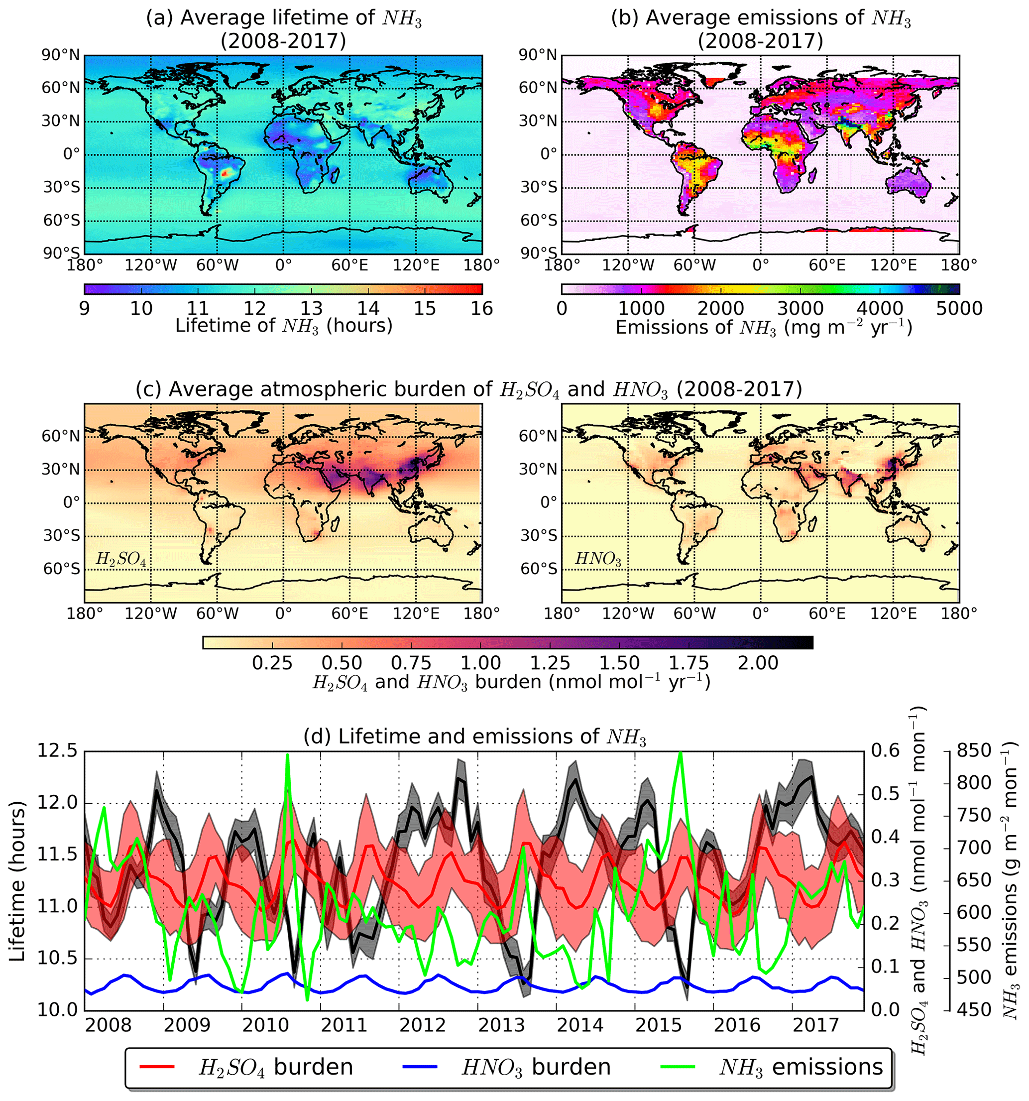
Figure 1(a) The 10-year average model lifetime of ammonia calculated from LMDz-OR-INCA; (b) total annual emissions averaged over the 10-year period (NE emissions); (c) atmospheric burden of the reactants sulfuric acid and nitric acid calculated in the model; and (d) monthly time series of lifetime (black), ammonia emissions (green), sulfuric (red) and nitric acid column concentrations (blue) for the whole 10-year period.
3.2 Satellite-constrained emissions
The average ammonia emissions calculated from the 10-year IASI observations are shown in Fig. 1b (also in Fig. S1a in the Supplement), the reactants' atmospheric burden in Fig. 1c and their seasonal variability in Fig. 1d together with monthly modelled lifetimes. The year-by-year total ammonia emissions are depicted in Fig. S1 with a monthly temporal resolution. Emissions decline from 242 Tg yr−1 in 2008 to 212 Tg yr−1 in 2011. During 2012–2014, emissions show little variation (194, 204 and 195 Tg yr−1, respectively) before they increase steeply to 248 Tg yr−1 in 2015. Finally, in 2016 and 2017 they remain at the same high level (197 and 227 Tg yr−1, respectively).
The global average annual emission calculated from VD0.5 amounts to 189 Tg (9-year average), which is comparable to the average of the 10-year period that we have calculated in the present study (average ± SD: 213 ± 18.1 Tg yr−1). The increase in the emissions we calculate during 2015 and 2017 stand out. The explanation for these increases could be twofold: (i) if sulfur dioxide (a precursor of sulfuric acid) emissions decreased over time, less sulfuric acid is available to neutralize ammonia, hence resulting in higher ammonia column concentrations seen by IASI that could be attributed to new emissions erroneously (see Sect. 2.4); (ii) if sulfur dioxide and sulfuric acid presented a constant year-by-year pattern or even increased, then the calculated ammonia emissions would be likely real.
To sort out these two possibilities, we used sulfur dioxide measurements from NASA's Ozone Monitoring Instrument (OMI; Yang et al., 2007), whereas sulfate column concentrations were taken from the Modern-Era Retrospective analysis for Research and Applications, Version 2 (MERRA-2; Gelaro et al., 2017) reanalysis data from NASA's Global Modeling and Assimilation Office (GMAO). Figure S2 shows time series of column concentrations of sulfur dioxide and sulfates from OMI and MERRA-2 averaged globally, for continental regions (Europe, North America, South America, Africa), as well as for regions where ammonia emissions are particularly high (India and Southeastern Asia, North China Plain). Although column concentrations of both sulfur dioxide and sulfates present strong interannual variability (Fig. S2), their global concentrations show a strong decreasing trend after 2015. The observed decrease indicates that sulfate neutralizes ammonia and forms ammonium sulfate; thus, it is likely that the higher ammonia concentrations seen from IASI after 2015 are not necessarily a result of emission increases. This is not seen from the respective precursor of the atmospheric nitric acid, i.e. nitrogen dioxide (Fig. S2). Sulfur dioxide emissions over Europe and North America have been reduced by 70 %–80 % since 1990 (Vestreng et al., 2007). The largest emission reductions occurred in North America after 2005 (Hand et al., 2012; Hoesly et al., 2018; Lehmann et al., 2007; Sickles and Shadwick, 2015) and in Europe before 2000 (Crippa et al., 2016; Hoesly et al., 2018; Torseth et al., 2012; Vestreng et al., 2007). These large regional reductions of sulfur dioxide resulted in a global decrease until 2000; they then slightly increased until 2006, due to a sharp rise in emissions in China, and declined again, due to stricter emission restrictions in China (Klimont et al., 2013; Li et al., 2017, 2018; Saikawa et al., 2017a; Wang et al., 2017; Xing et al., 2015; Zhang et al., 2012; Zheng et al., 2018) and regulations in Europe and North America (Aas et al., 2019; Crippa et al., 2016; Hoesly et al., 2018; Klimont et al., 2013; Reis et al., 2012). This was not the case for India, where the emissions have been increasing (Hoesly et al., 2018; Klimont et al., 2017; Saikawa et al., 2017b), making it the world's second largest sulfur dioxide emitting country after China (Krotkov et al., 2016).
Looking closely into regions with large changes in ammonia's reactants and/or their precursors after 2015 (Fig. 2), we immediately see that a region of interest is the North China Plain. The North China Plain has been identified as an ammonia hot-spot mainly due to extensive agricultural activities (Clarisse et al., 2009; Pan et al., 2018). To improve air quality over China, the Chinese government implemented new emission regulations aimed at decreasing the national total NOx emissions by 10 % between 2011 and 2015 (Liu et al., 2017). Several recent studies (Duncan et al., 2016; Krotkov et al., 2016) have highlighted the effectiveness of the air quality policy, as evidenced by a decreasing trend in nitrogen dioxide columns over China since 2012. De Foy et al. (2016) reported that NOx reduction goals had already been achieved in 2016, as seen from satellites. A similar decreasing trend has been reported for sulfur dioxide (Koukouli et al., 2018; Krotkov et al., 2016; Wang et al., 2013). For instance, Liu et al. (2018) reported a sulfur dioxide reduction of about 60 % over the recent few years in the North China Plain: sulfuric acid decreased by 50 %, while ammonia emissions declined by only 7 % due to change in agricultural practices.
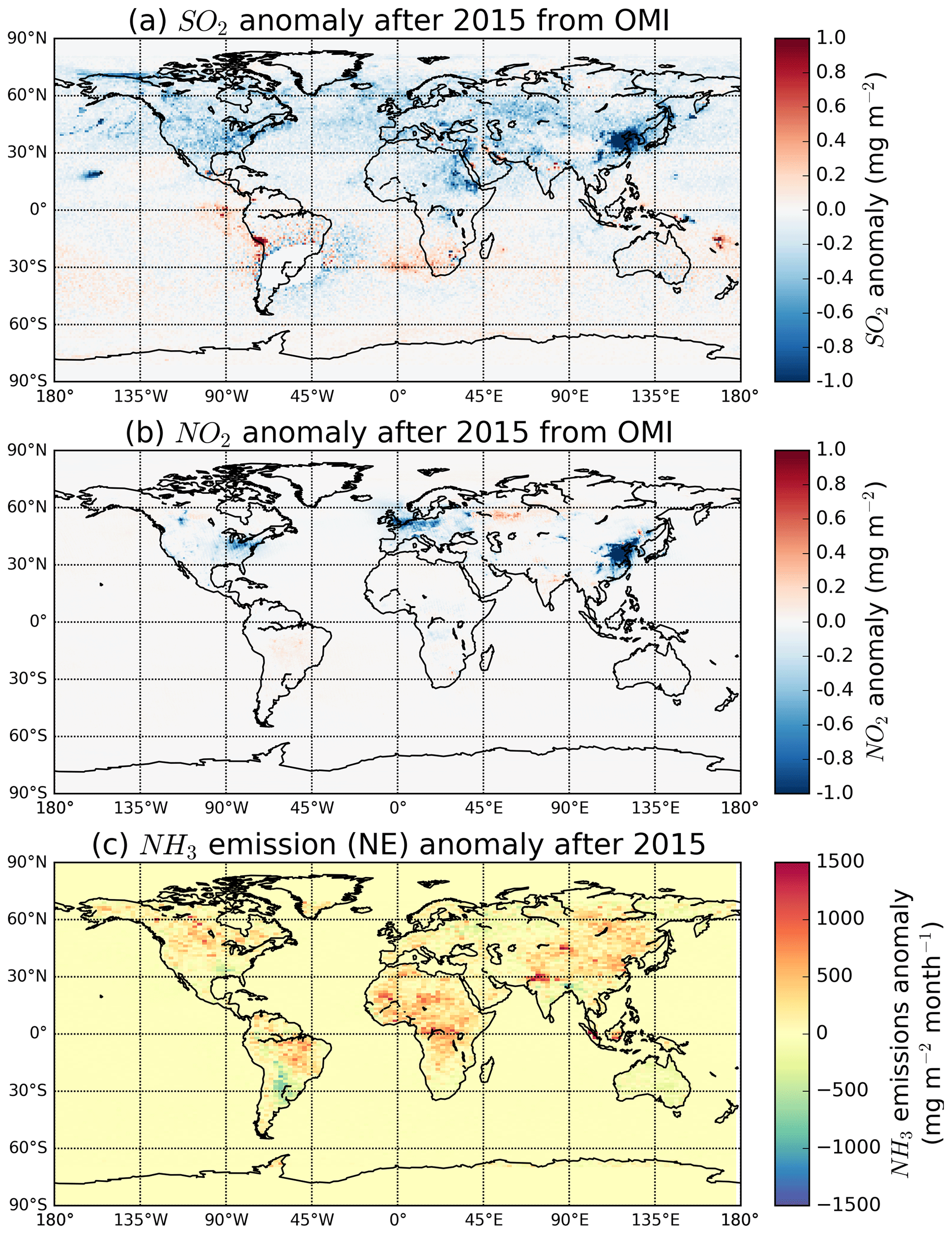
Figure 2Annual average total column (a) sulfur dioxide and (b) nitrogen dioxide anomaly after 2015 from OMI and (c) annual average emission anomaly of ammonia calculated from IASI in the present study (NE).
The suggested decrease in ammonia reactants over the North China Plain is illustrated by the calculated sulfur dioxide column concentration anomaly from OMI (Fig. 2) and by the sulfuric acid concentration anomaly from MERRA-2 after 2015 (the highest calculated one) (Fig. S3). Nitrogen dioxide concentration do not show any noticeable annual change, despite their strong seasonal cycle (Fig. S2). The IASI-constrained ammonia emissions calculated here show only a tiny increase of 0.19±0.04 kt yr−1 after 2015 in the North China Plain and of 10±3.1 Tg yr−1 globally with respect to the 10-year average (Fig. 2). This is due to the change of sulfur dioxide and nitrogen oxide emission regulations in China, which in turn led to reduced inorganic matter (sulfates, nitrates and ammonium), resulting in regional increases of gaseous ammonia (Lachatre et al., 2019).
It should be noted here that decreases in sulfur dioxide and nitrogen dioxide have been reported to have occurred since 2005, at least in eastern USA and to a lesser extent in eastern Europe (Krotkov et al., 2016). At the same time, sulfur dioxide and nitrogen dioxide concentrations had started increasing after 2005 in India, which is a country that shows the largest agricultural activity in the world and is now the second largest sulfur dioxide emitting country after China (Krotkov et al., 2016). The latter has balanced the global sulfur dioxide and nitrogen dioxide budget, explaining that the decreasing trend after 2015 that we report has been affected by our choice to present global averages.
3.3 Comparison with traditional emission datasets
In this section, we quantify the main differences of our IASI-constrained emission dataset with other state-of-the-art inventories used in global models and for different applications (air quality, climate change, etc.). Aside from comparing our emissions with those calculated using Van Damme et al. (2018) data with a constant lifetime (hereafter called VD0.5), we extend our comparison to more traditional datasets such as those of ECLIPSEv5-GFED4-GEIA (EGG) for 2008–2017 and EDGARv4.3.1-GFED4 (Crippa et al., 2016; Giglio et al., 2013) for the 2008–2012 period. Finally, the ammonia emissions presented in this study (NE emissions) are compared to emissions calculated from Van Damme et al. (2018) gridded IASI column data applying a variable (modelled) ammonia lifetime presented in Fig. 1b (hereafter referred to as VDgrlf).
The 10-year comparison of our calculated emissions with VD0.5 is shown in Fig. 3. The 10-year average difference amounts to 29±15 Tg yr−1 (average ± SD). In all years, the largest differences could be seen over Latin America and over tropical Africa. Our emissions (NE) show a different structure in the Indo-Gangetic Plain and situated slightly more northerly than those in VD0.5. The difference might be due to the IDW interpolation used to process the IASI ammonia in the NE emissions compared with the oversampling method used in VD0.5 (see Sect. 2.3). Nevertheless, northern India has been identified as a hot-spot region for ammonia, mainly due the importance of agricultural activities in the region (Kuttippurath et al., 2020; Tanvir et al., 2019).
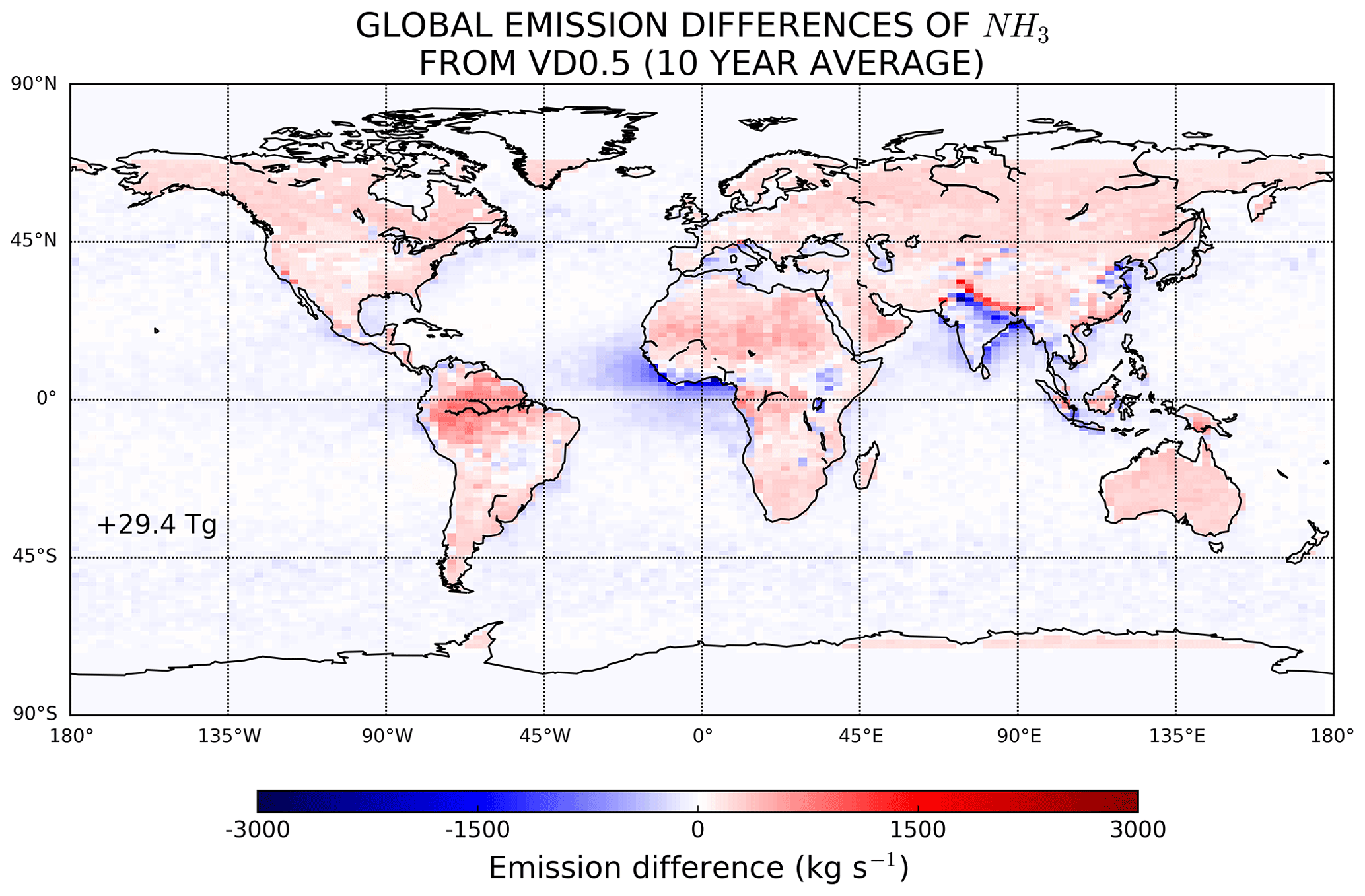
Figure 3Global differences of ammonia emissions calculated in the present study (NE) from those calculated using Van Damme et al. (2018) gridded concentrations applying a constant lifetime of 0.5 d (VD0.5). The results are given as 10-year average (2008–2017), and the number denotes the annual difference in the emissions.
Figures S4 and S5 present a comparison of our calculated emissions (NE) with the basic state-of-the-art datasets of EGG and EDGARv4.3.1-GFED4, respectively. In both datasets, ammonia emissions remain almost constant over time (average ± SD: 65 ± 2.8 Tg yr−1 and 103 ± 5.5 Tg yr−1, respectively). The total calculated ammonia emissions in EGG and EDGARv4.3.1-GFED4 are up to 3 times lower than those calculated from NE (average ± SD: 213 ± 18.1 Tg yr−1) or from VD0.5 (9-year average: 189 Tg yr−1). This results in 10-year annual differences that are very significant (average ± SD: 150 ± 19.3 and 111 ± 19.2 Tg yr−1, respectively); the largest differences appear over South America (EGG: 7.1 ± 0.3 Tg yr−1, VD0.5: 22 Tg yr−1, NE: 28 ± 3.0 Tg yr−1, VDgrlf: 24 ± 1.3 Tg yr−1), while European emissions are practically identical in all datasets except EGG (EGG: 6.9 ± 1.1 Tg yr−1, VD0.5: 11 Tg yr−1, NE: 15 ± 2.2 Tg yr−1, VDgrlf: 11 ± 1.0 Tg yr−1). Emissions from North China Plain are much higher in the two traditional datasets than those presented in this paper (EGG: 25 ± 1.2 Tg yr−1, VD0.5: 36 Tg yr−1, NE: 38 ± 2.8 Tg yr−1, VDgrlf: 39 ± 1.8 Tg yr−1). Ammonia emissions derived over China in this work (NE) are among the highest worldwide (Fig. S1), which agrees well with the 9-year average emissions calculated in the VD0.5 inventory over China (see Fig. 3). To assess to which extent emissions from EGG and EDGARv4.3.1-GFED4 are underestimated can only be done by comparing ammonia with ground or satellite observations.
The comparison of the annual ammonia emissions in the NE dataset to the modified VDgrlf emissions is shown in Fig. S6. The latter showed a better agreement to the emissions presented in this study with mean annual difference of 14 ± 19 Tg yr−1 (average ± SD). Previously observed emission differences in the two state-of-the-art inventories over South America and Africa have been now minimized, and the displacement north of the Indo-Gangetic Plain emissions remains important. Nevertheless, the smaller differences of our emissions (NE) from those of VDgrlf as compared with the respective difference from the VD0.5 emissions show the large impact that a more realistic variable lifetime might have in emission calculations with this methodology in these regions.
3.4 Region-specific ammonia emissions and seasonal variation
Figure 4 illustrates specific regions that show the largest ammonia emissions (Europe, North America, South America and Southeastern Asia). These emissions correspond to the IASI-constrained emissions calculated in this study (NE) and are presented as total annual emissions averaged over the 10-year period of study. In the bottom panels of the same figure, the seasonal variation of the emissions is shown for each of the four hot-spot regions and each of the 10 years of the study.
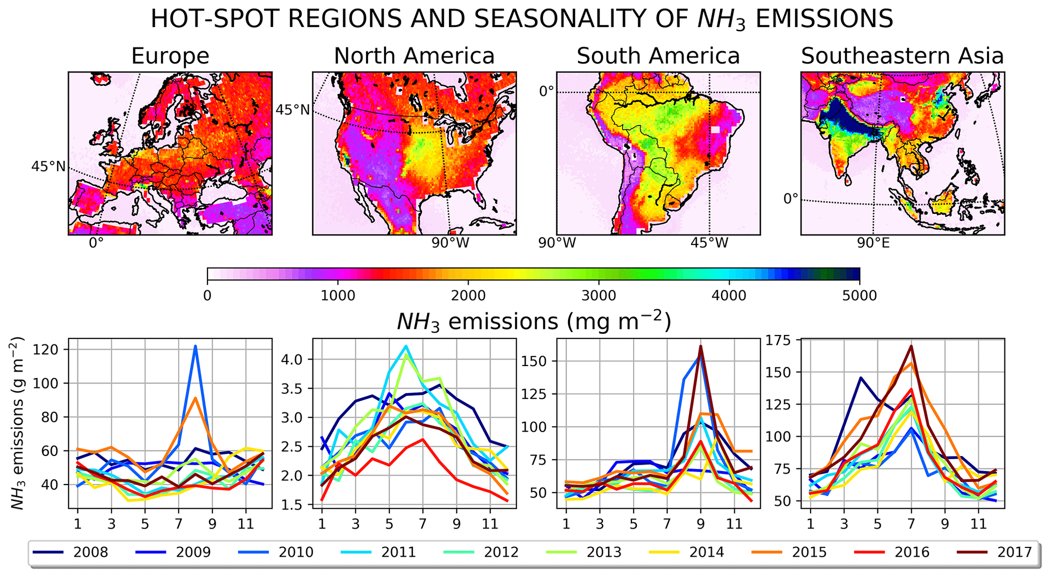
Figure 4Total annual emissions of ammonia averaged over the 10-year period (2008–2017) in Europe, North America and South America, and Southeastern Asia, which are regions characterized by the largest contribution to the global ammonia budget. In the bottom panels the monthly variation of the emissions is shown for each year of the study periods.
European total ammonia emissions were estimated to be 15 ± 2.2 Tg yr−1 (average ± SD), which are more than double compared with those reported in EGG (6.9 ± 1.1 Tg yr−1) and similar to those in VD0.5 (11 Tg yr−1) or those in VDgrlf (11 ± 1.0 Tg yr−1). The greatest emissions were calculated for Belgium, the Netherlands and the Po Valley in Italy (Fig. 4). High emissions are also found in north and northwestern Germany and over Denmark. In contrast, very low emissions are found in Norway, Sweden and parts of the Alps. It is not possible to quantitatively distinguish between different sources of ammonia. It has been reported that approximately 75 % of ammonia emissions in Europe originate from livestock production (Webb et al., 2005), and 90 % from agriculture in general (Leip et al., 2015). More specifically, ammonia is emitted at all stages of manure management: from livestock buildings during manure storage, application to land and from livestock urine. These emissions are strong over most northwest European countries, although sources like fertilization and non-agricultural activities (traffic and urban emissions) can be also important. An example is Tange in Germany, which shows a late summer peak due to application of growing crops. No obvious seasonality in the emissions can be seen for Europe as a whole, as the hot-spot regions are rather few compared to the overall surface of Europe. An exception to this stable emission situation over the year occurs during 2010 and during 2015, years for which there is a late summer peak. In 2010, large wildfires in Russia resulted in high ammonia emissions (R'Honi et al., 2013), while year 2015 has been also characterized as an intense fire year (although not like 2010), with fires occurring in Eurasia (Min Hao et al., 2016).
North America and in particular the US (Fig. 4) has been characterized by four hot-spot regions. First, a small region in Colorado, USA, which is the location of a large agricultural region that traditionally releases large ammonia emissions (Malm et al., 2013). Another example is the state of Iowa (home to more than 20 million swine, 54 million chickens, and 4 million cattle), northern Texas and Kansas (beef cattle), and southern Idaho (dairy cattle) (McQuilling, 2018). Furthermore, the three major valleys in Salt Lake City, in Cache, and in Utah in the midwestern US show an evident, but lower intensity hot-spot, as they are occupied by massive pig farms associated with open waste pits. The largest emissions were calculated for the San Joaquin Valley in California (vegetables, dairy, beef cattle and chickens) and further to the south (Tulare and Bakersfield), which is an area characterized by feedlots (Van Damme et al., 2018; McQuilling, 2018). North American annual ammonia emissions over the 10-year period were averaged 1.1 ± 0.1 Tg yr−1 (average ± SD). These values are over 2 orders of magnitude higher than those in EGG (0.062 ± 0.0013 Tg yr−1). Note that their estimate is 3 times lower than those reported in VD0.5 (3.1 Tg yr−1) or in VDgrlf (3.4 ± 0.5 Tg yr−1). The 2008–2017 interannual variability data (Fig. 4) all show a minimum in winter. Maximum emissions were observed in late spring, due to the contribution from mineral fertilizer and manure application; in summer, due to influence of livestock housing emissions; and some years both in spring and summer (Makar et al., 2009; Zhu et al., 2013, 2015). A topographical dependence was also seen in midwest emissions that peaked in April, whereas over the rest of the US maximum emissions appeared in summer (Paulot et al., 2014).
Ammonia emissions have different characteristics in South America and in western Africa as both are fire-dominated regions. For simplicity we only present South America in Fig. 4. This region is dominated by natural ammonia emissions mainly from forest, savanna and agricultural fires (Whitburn et al., 2014, 2016b) as well as volcanoes (Kajino et al., 2004; Uematsu et al., 2004). This causes a strong seasonal variability in the ammonia emissions with the largest fluxes observed from August to October in all years (Fig. 4). This strong dependence of South America from biomass burning emissions was first highlighted by Chen et al. (2013) and by van Marle et al. (2017). It also became particularly pronounced during the large wildfires in the Amazon rainforest in summer 2019 (Escobar, 2019). We estimated the 10-year average ammonia emissions to be 28 ± 3.0 Tg yr−1 (average ± SD) in agreement with VD0.5 (22 Tg yr−1) and VDgrlf (24 ± 1.3 Tg yr−1). The respective emissions in EGG are 4 times lower than these estimates (7.1 ± 0.3 Tg yr−1).
The last column to the right of Fig. 4 presents the 10-year average annual ammonia emissions and their respective interannual variability in Southeastern Asia. We define this region spanning from 70–130∘ E in longitude and from 0–45∘ N in latitude. Ammonia emissions were estimated to be 38 ± 2.8 Tg yr−1 (average ± SD) similar to VD0.5 (36 Tg yr−1) and VDgrlf (39 ± 1.8 Tg yr−1) and slightly higher than those presented in EGG (25 ± 1.2 Tg yr−1). They comprise ammonia fertilizer plants, such as in Pingsongxiang, Shizuishan, Zezhou-Gaoping, Chaerhan Salt Lake , Delingha, Midong-Fukang and Wucaiwan (China), Indo-Gangetic Plain (Pakistan and India), and Gresik (Indonesia). China and India contribute more than half of total global ammonia emissions since the 1980s with the majority of these emissions originating from rice cultivation followed by corn and wheat (crop-specific emissions). More specifically, emissions from these crops due to synthetic fertilizer and livestock manure applications are concentrated in the North China Plain (Xu et al., 2018). Considering that Southeastern Asia is the largest agricultural contributor in the global ammonia budget, a strong seasonality in the emissions was observed. Temporal ammonia emissions peak in late summer of most years, when emissions from rice cultivation, synthetic fertilizer application and livestock manure spreading (Xu et al., 2016) are important, as well as in spring when wheat cultivation dominates (Datta et al., 2012). Of course, the respective emissions from biomass burning should also be mentioned. However, these are difficult to distinguish and are expected to be a relatively small source compared to agricultural emissions.
In this section, we conduct simulations over the 10-year period (2008–2017, 1-year spin-up), with all the emissions derived, and compare the NH3 concentrations with ground-based observations over Europe, North America, Southeastern Asia (Sect. 4.1) and satellite observations from CrIS (Sect. 4.1). These simulations consist of (i) a simulation using traditional emissions using EGG; (ii) a simulation using emissions calculated from IASI data from Van Damme et al. (2018) applying a constant lifetime of 12 h for ammonia (VD0.5); (iii) a simulation using gridded emissions presented in the present paper (NE) calculated as described in Sect. 2; and (iv) a simulation using emissions calculated from IASI data from Van Damme et al. (2018) applying a variable (modelled) lifetime (VDgrlf). Finally, we perform a sensitivity analysis in order to define the levels of uncertainty of our emissions in Sect. 4.3 and discuss potential limitations of the present study in Sect. 4.4.
4.1 Validation against ground-based observations and satellite products
Figure 5 shows a comparison between modelled surface concentrations of ammonia with ground measurements from Europe (EMEP, https://emep.int/mscw/, last access: 17 February 2021), North America (AMoN, http://nadp.slh.wisc.edu/data/AMoN/, last access: 17 February 2021) and Southeastern Asia (EANET; https://www.eanet.asia, last access: 17 February 2021). To avoid overplotting, the Gaussian kernel density estimation (KDE) was used, which is a non-parametric way to estimate the probability density function (PDF) of a random variable (Parzen, 1962):
where K is the kernel, xi the univariate independent and identically distributed point of the relationship between modelled and measured ammonia, and h is a smoothing parameter called the bandwidth. KDE is a fundamental data smoothing tool that attempts to infer characteristics of a population, based on a finite dataset. It weighs the distance of all points in each specific location along the distribution. If there are more points grouped locally, the estimation is higher as the probability of seeing a point at that location increases. The kernel function is the specific mechanism used to weigh the points across the data set, and it uses the bandwidth to limit the scope of the function. The latter is computed using Scott's factor (Scott, 2015). We also provide the mean fractional bias (MFB) for modelled and measured concentrations of ammonia as follows:
where Cm and Co are the modelled and measured ammonia concentrations, respectively, and N is the total number of observations. MFB is a symmetric performance indicator that gives equal weights to under- or overestimated concentrations (minimum to maximum values range from −200 % to 200 %). Furthermore, we assess the deviation of the data from the line of best fit using the root mean square error (RMSE) defined as
From 134 European stations, nearly 300 000 measurements made at a daily to weekly temporal resolution over the period of study (2007–2018) are presented in Fig. 5. All emission datasets underestimate ammonia surface concentration over Europe. The most accurate prediction of concentrations was achieved using the traditional EGG emissions that underestimated observations by 67 %, also being the least scattered from the best fit (RMSEEGG=4.06 µg N m−3), followed by the emissions presented in this paper ( %, RMSENE=4.65 µg N m−3), although they were more variable. VD0.5 or VDgrlf emissions further underestimated observations, although they were less sparse (Fig. 5d). About 12 % of the modelled concentrations using EGG were outside of the 10-fold limit from the observations, in contrast to only 17 % and 15 % in VD0.5 and VDgrlf and 20 % in NE. In regard to the spatial comparison with the observed concentrations, all datasets cause overestimations in the ammonia concentrations predicted in western Europe. EGG appears to be the most accurate in central Europe (all stations with suffix DE00), NE emissions in all Spanish stations (suffix ES00) and VD0.5 and VDgrlf emissions in Italian stations (Fig. S7).
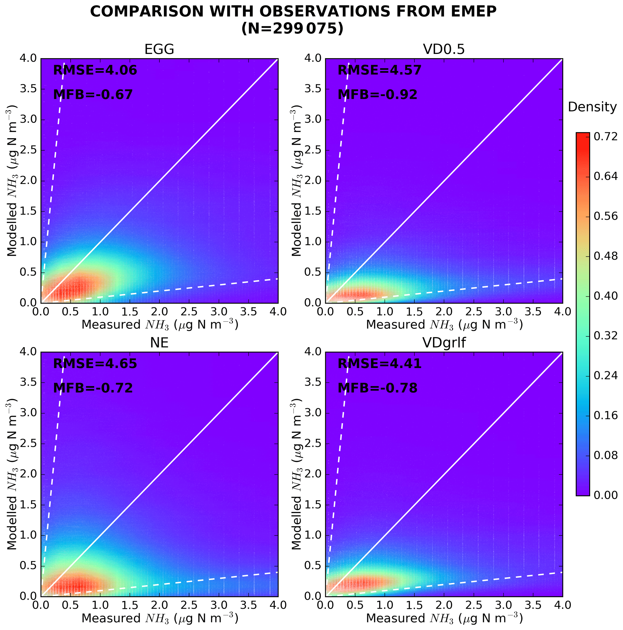
Figure 5Validation of modelled concentrations of ammonia for different emissions datasets (EGG, VD0.5, NE and VDgrlf) against ground-based measurements from EMEP for the 10-year (2008–2017) study period. Scatterplots of modelled against measured concentrations for the aforementioned emission inventories were plotted with the Kernel density estimation, which is a way to estimate the probability density function (PDF) of a random variable in a non-parametric way.
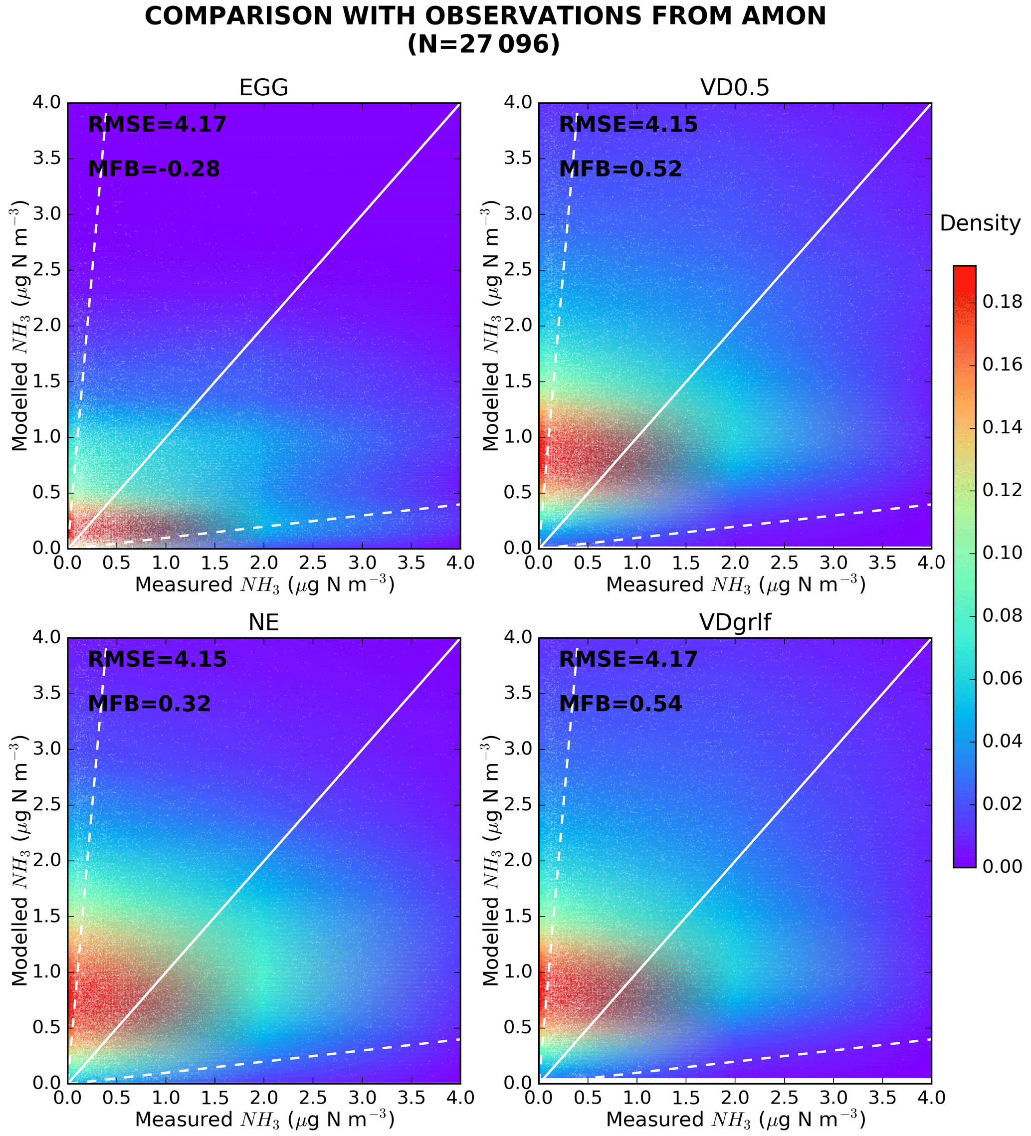
Figure 6Validation of modelled concentrations of ammonia for different emissions datasets (EGG, VD0.5, NE and VDgrlf) against ground-based measurements from AMON for the 10-year (2008–2017) study period. Scatterplots of modelled against measured concentrations for the aforementioned emission inventories were plotted with the Kernel density estimation, which is a way to estimate the probability density function (PDF) of a random variable in a non-parametric way.
The comparison of simulated ammonia concentrations to observations over North America includes 119 stations, which represent nearly 27 000 observations (Fig. 6) with a weekly, biweekly or monthly resolution. The only emission dataset that lead to an underestimation of ammonia concentrations was EGG ( %). Two others, VD0.5 and VDgrlf, caused ammonia observations to be strongly overestimated (MFBVD0.5=52 % and MFBVDgrlf=54 %), while NE only slightly (MFBNE=32 %). All inventories resulted in about the same variability in ammonia concentrations with RMSEs between 4.15 and 4.17 µg N m−3 (Fig. 6). About 10 % of the predicted concentrations using EGG emissions were at least 10 times off from the measured ones, which is more than twice the number of measurements compared to the other dataset. NE emissions better capture levels in the easternmost stations of the US (AL99, AR15, CT15, IL37, IN22, MI52, NY56, ON26) and in California (CA83) and Oklahoma (OK98), which are close to hot-spot regions (see Sect. 3.4). EGG emissions perform better in northwestern (ID03), central (KS03) and several stations located over the eastern United States (KY03, KY98, OH09, AR03, IL46, KS03, GA41). The emission inventory VD0.5 leads to a very good agreement in ammonia concentrations over all stations of the North American continent (AL99, GA40, ID03, GA41, IL37, IL46, IN20, IN22, KS97, PA00, MD99, MI52, TN04, NM99, NY96, OH99, OK98) (Fig. S8).
In Southeastern Asia 62 stations from 13 countries were included in the comparison from the EANET monitoring network (Fig. 7). These included about 8000 surface measurements in monthly or 2-weekly resolution. As a whole, all emission inventories underestimate station concentrations of EANET with MFBs between −102 % (EGG) and −61 % (VD0.5 and VDgrlf). The least spread model concentrations were those simulated using VD0.5 and VDgrlf (RMSE = 461–465 µg N m−3). Around 19 % of model concentrations using EGG were outside the 10-fold limit of the 1×1 line with observations, 12 % using NE emissions, and only 5 % and 6 % using VD0.5 and VDgrlf, respectively. VD0.5 and VDgrlf emissions capture well the Japanese (suffix JPA) and Taiwanese stations (suffix THA). Given the short lifetime and the relatively coarse spatial scales, the model fails to capture the variability that exists within each grid box (Fig. S9).
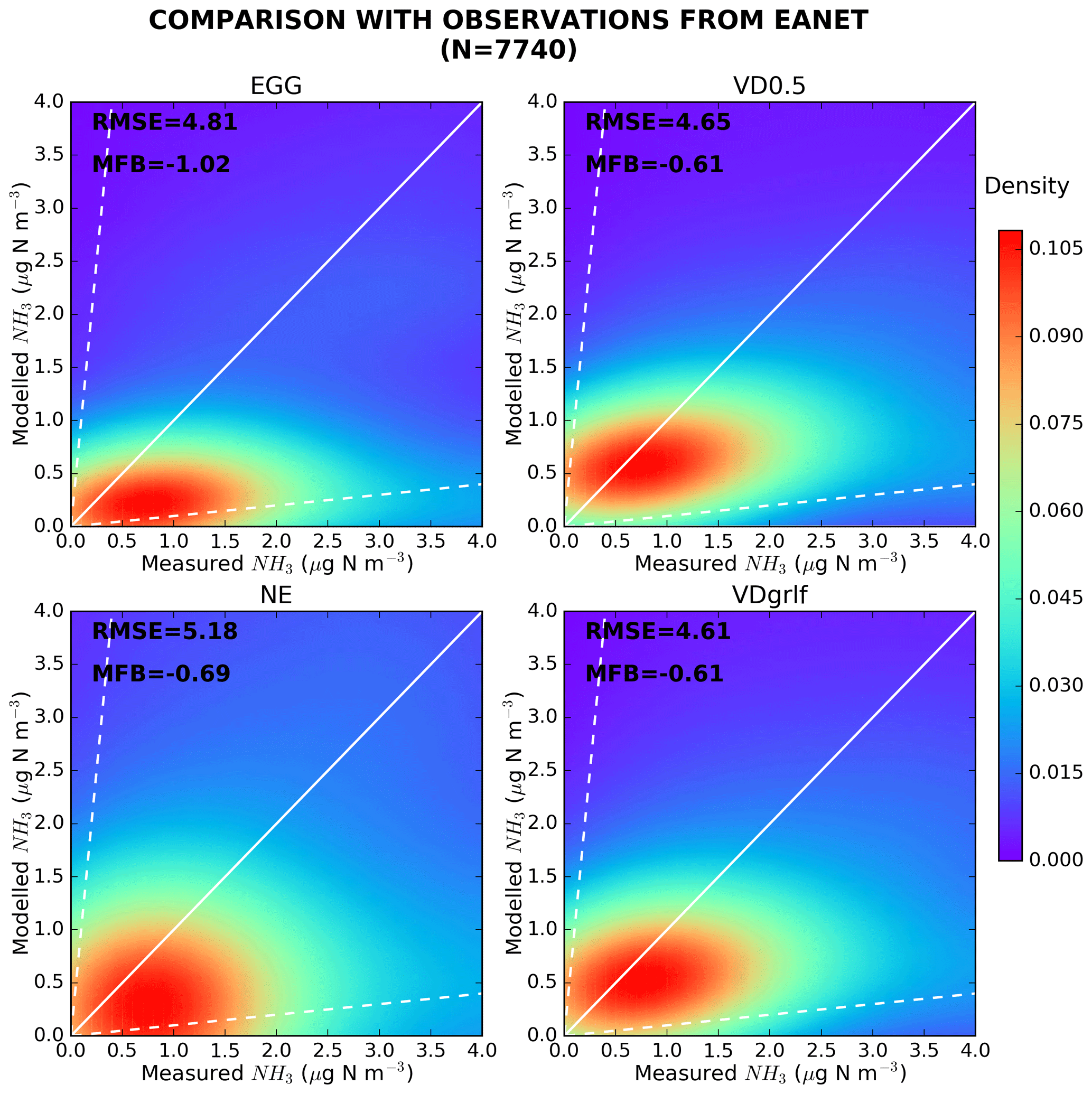
Figure 7Validation of modelled concentrations of ammonia for different emissions datasets (EGG, VD0.5, NE and VDgrlf) against ground-based measurements from EANET for the 10-year (2008–2017) study period. Scatterplots of modelled against measured concentrations for the aforementioned emission inventories were plotted with the Kernel density estimation, which is a way to estimate the probability density function (PDF) of a random variable in a non-parametric way.
To give an overview of the comparison of the modelled surface concentrations of ammonia from the four different simulations, each with different emissions (EGG, VD0.5, NE and VDgrlf), we present station-by-station calculated MFB values in Fig. 8. Although the traditional EGG emissions capture many stations very well, there are large MFB values observed in eastern and western USA (AMoN) and northern Europe (EMEP), whereas large overestimations are observed in most of the Southeastern Asian stations (EANET). The large bias at several AMoN stations decreases when using satellite-derived emissions. All datasets miscalculated surface concentrations in Southeastern Asia, although some stations present lower MFBs when using IASI constrained emissions. Note that large differences when comparing bias from all measurements versus station-by-station bias have been calculated as a result of the different frequencies of measurements in each station.
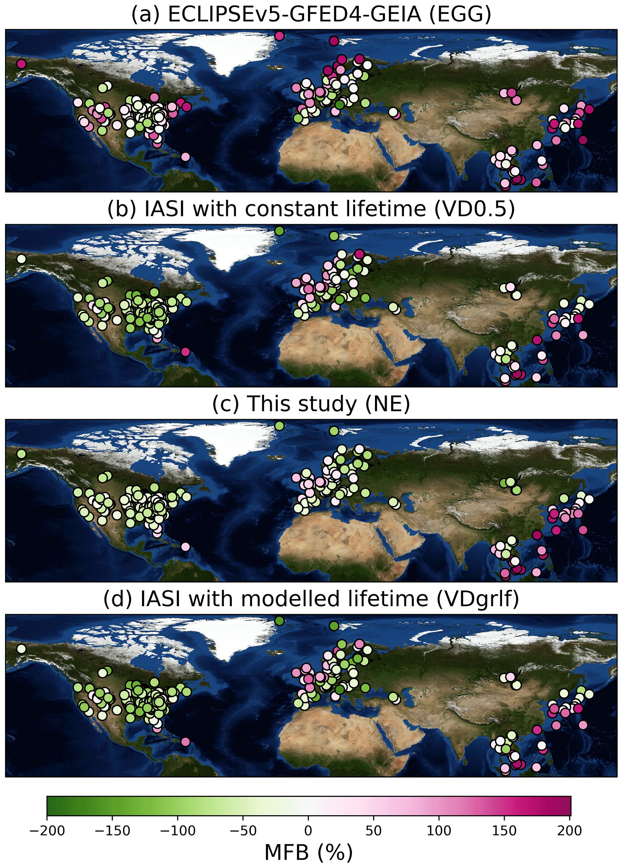
Figure 8Overview of the comparison with ground-based measurements of ammonia. MFB for each of the stations from AMoN, EMEP and EANET monitoring stations calculated after running LMDz-OR-INCA with the emissions of EGG, VD0.5, NE and VDgrlf for the period 2008–2017.
To further show whether the satellite-derived emissions presented here (NE) capture surface concentrations of ammonia or not, we used surface ammonia concentrations from CrIS from 1 May 2012 to 31 December 2017. The comparison is shown as PDF of surface modelled against CrIS concentrations of ammonia calculated with the Gaussian KDE for North America, Europe and Southeastern Asia in Fig. 9. NE emissions slightly overestimate ammonia (MFB = 0.09–0.10). NE emissions generally result in higher surface concentrations, also showing large RMSEs (3.28–5.26 µg N m−3). However, 90 % of the modelled concentrations were within a factor of 10 from the CrIS observation.
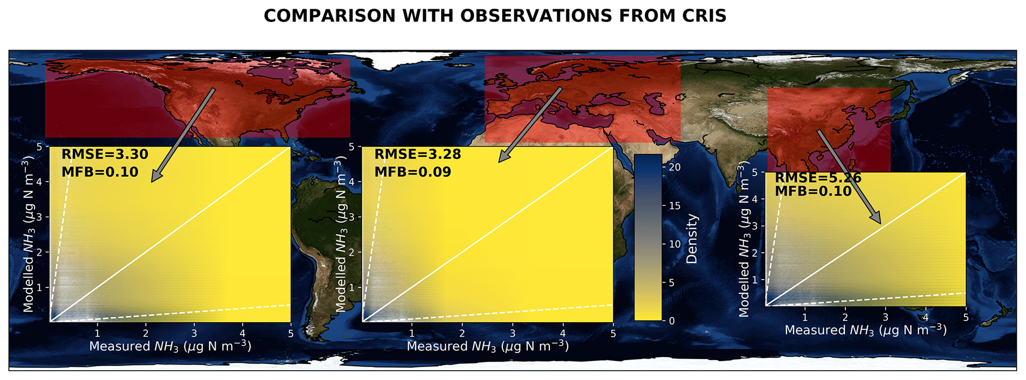
Figure 9Kernel density estimation (KDE) of the probability density function (PDF) of modelled versus CrIS concentrations of ammonia in a non-parametric way. Modelled concentrations are results of simulations using NE emissions datasets for the period 2012–2017, for which CrIS data were available. The comparison is shown for North America, Europe and Southeastern Asia.
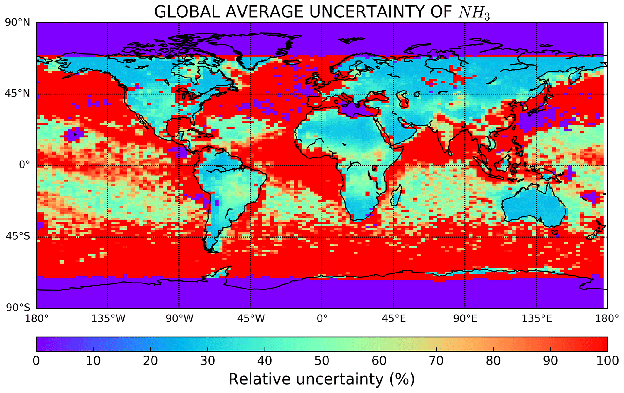
Figure 10The 10-year average relative uncertainty of modelled surface concentrations expressed as the standard deviation of surface concentrations from a model ensemble (Table 1) divided by the average.
4.2 Uncertainty analysis
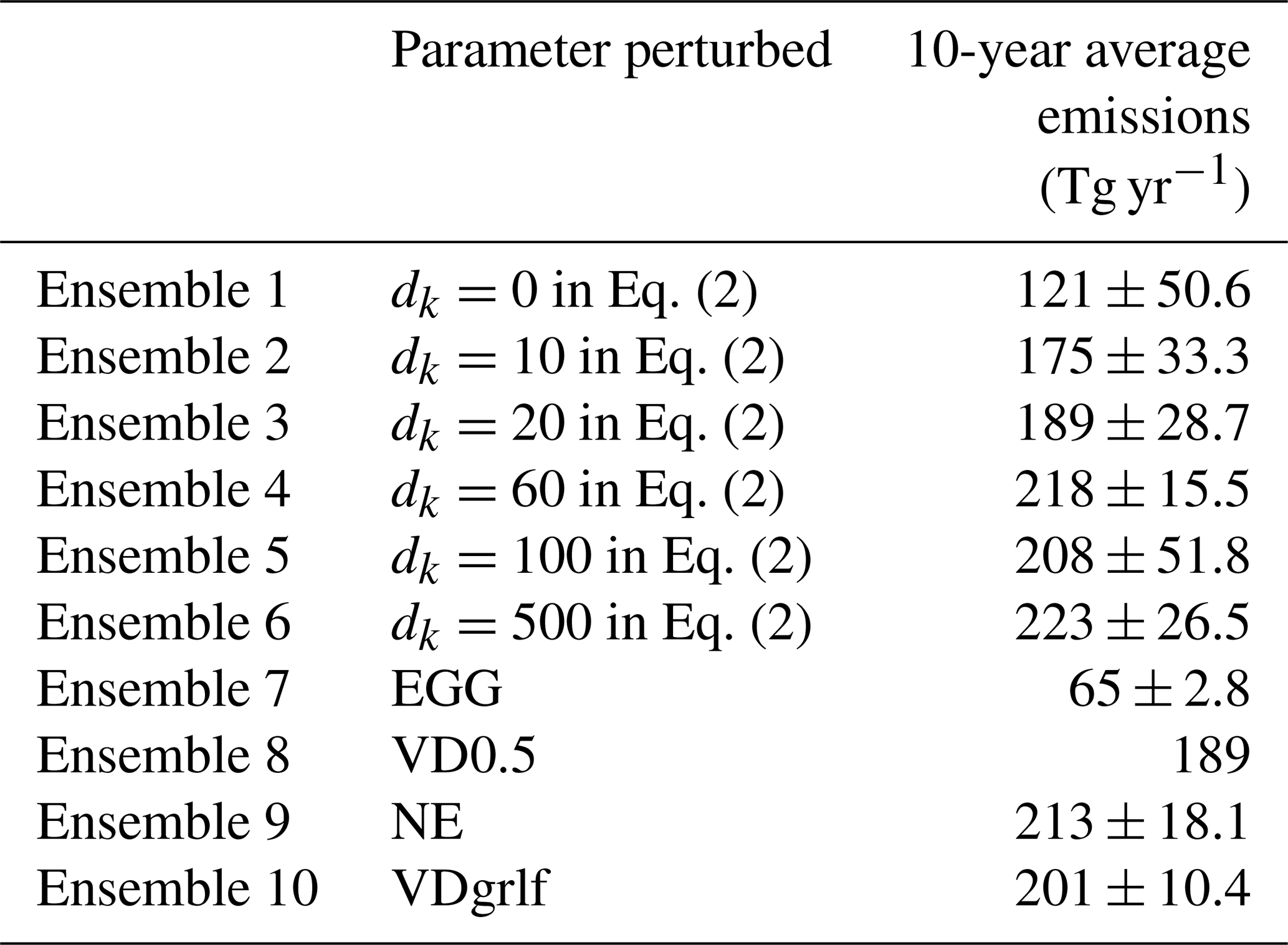
A sensitivity analysis was also performed in order to calculate the level of uncertainty that each of the parameter gives to the modelled surface concentrations of ammonia. The relative uncertainty was calculated as the standard deviation of ammonia's surface concentrations from a model ensemble of 10 members (Table 1) divided by the average. The first six members are the surface concentrations that resulted from simulations of ammonia emissions after perturbation of the Euclidian distance dk in the parameters of the IDW interpolation. The remaining four members are simulated concentrations using the previously reported emissions datasets (EGG, VD0.5, NE and VDgrlf). The results are shown as a 10-year (2008–2017) annual average relative uncertainty in Fig. 9 and as annual average relative uncertainty of surface concentrations for every year of the 10-year period in Fig. S10.
Table 1Model ensemble simulations using different emissions for ammonia that were used in the calculations of uncertainty. Uncertainties were calculated as the standard deviation of the surface concentrations of ammonia from the 10 ensemble members for the 10-year period (2008–2017).
The surface concentrations resulting from the different calculated emissions mainly affects oceanic regions, with relative uncertainties reaching 100 % (Fig. 10). The reason for this could be threefold. First, the IDW interpolation shows it to be affected by severe outlier values, which are found in several oceanic regions (Fig. S11); this creates high gridded column ammonia concentrations and, in turn, fluxes at regions that are not supported by previous findings or measurements. Second, the methodology with which ammonia concentrations are retrieved in IASI has certain limitations, with respect to (i) the use of constant vertical profiles for ammonia, (ii) potential dependencies of total column ammonia and temperature that are not taken into account, and (iii) instrumental noise that can cause bias (Whitburn et al., 2016a). Third, there is much less ammonia over the Ocean; hence, the relative error bars are much larger. Large uncertainties in surface ammonia concentrations were observed in regions characterized by large anthropogenic contribution, such as northern India, North China Plain and central USA. Smaller uncertainties were found in central Africa and in Amazonia, which are regions linked with episodic biomass burning emissions (Fig. 4).
4.3 Limitations of the present study
We discuss the importance of certain limitations in the methodology of the present study and in the validation of the results. These limitations will also be commented on in the overall conclusion of the paper.
Regarding the methodology, emissions of short-lived species are determined, among other methods, using top-down approaches. When only satellite measurements are available, they are usually averaged over a particular location, and surface emissions are calculated using a mass balance approach (Lin et al., 2010; Zhao and Wang, 2009). This is done by assuming a one-dimensional box model, where atmospheric transport between grids is assumed to be negligible, and loss due to deposition or chemical reactions is very fast. The solution to this problem is the use of kernels (Boersma et al., 2008), which makes the computation of the emissions very intense. It has been reported that for resolutions such as those used in the present paper (2.5∘ × 1.3∘), non-local contributions to the ammonia emissions are relatively small (Turner et al., 2012). Although the use of kernels is the proper way to account for non-local contributions, we believe that negligible transport here is a fair assumption, due to the small lifetimes of ammonia calculated from the CTM (11.6 ± 0.6 h); therefore, transportation from the adjacent grid cells should be small. Note that although this method has been suggested for short-lived climate pollutants, it is not suitable for species with lifetimes from days to weeks (e.g. black carbon; Bond et al., 2013). Another important process that is not yet considered in our model is the treatment of ammonia's air–surface exchange. Although bidirectional air–surface exchange (dry deposition and emission) of ammonia has been observed over a variety of land surfaces (grasslands, tree canopies, etc.), the majority of the CTMs treat the air–surface exchange of ammonia as dry deposition only. This might cause underestimation of the daytime ambient ammonia concentration due to the overestimated dry deposition, considering that the observed bidirectional exchange of ammonia mainly occurs during the daytime (see Zhang et al., 2010, and references therein).
Another limitation of the present study is that the same model is used for the calculation of the modelled lifetimes and for the validation of the emissions that were calculated using these lifetimes (NE and VDgrlf). A more accurate validation would require an independent model for the simulations of surface concentrations using these emissions. Nevertheless, the IASI-constrained emissions of ammonia presented here are publicly available for use in global models.
In the present paper, satellite measurements from IASI were used to constrain global ammonia emissions over the period 2008–2017. The data were firstly processed to monthly ammonia column concentrations with a spatial resolution of 2.5∘ × 1.3∘. Then, using gridded lifetime for ammonia calculated with a CTM, monthly fluxes were derived. This contrasts with previously reported methods that used a single constant lifetime. This enables a more accurate calculation in regions where different abundances of atmospheric sulfuric and nitric acid, as well as in their precursors (sulfur and nitrogen dioxide, respectively), can neutralize ammonia through heterogeneous chemical reactions to sulfate and nitrate aerosols. The calculated ammonia emission fluxes were then used to simulate ammonia concentrations for the period 2008–2017 (referred to as NE). The same simulations were repeated using baseline emissions from ECLIPSEv5-GFED4-GEIA (referred to as EGG), emissions constrained by Van Damme et al. (2018) IASI data using a constant lifetime for ammonia (named as VD0.5) and emissions based on Van Damme et al. (2018) retrievals using a modelled lifetime from a CTM (named as VDgrlf). The simulated surface concentrations of ammonia were compared with ground measurements over Europe (EMEP), North America (AMoN) and Southeastern Asia (EANET), as well as with global satellite measurements from CrIS. The main conclusions can be summarized as follows:
The 10-year average annual ammonia emissions calculated here (NE) were estimated to be 213 ± 18.1 Tg yr−1, which is 15 % higher than those in VD0.5 (189 Tg yr−1) and 6 % higher than those in VDgrlf (201 ± 10.4 Tg yr−1). These emission values amount to twice as much as those published from datasets, such as EGG (65 ± 2.8 Tg yr−1) and EDGARv4.3.1-GFED4 (103 ± 5.5 Tg yr−1).
In the North China Plain, a region characterized by intensive agricultural activities, a small increase of ammonia emissions is simulated after 2015. This is attributed to decreases in sulfur species, as revealed from OMI and MERRA-2 measurements. Less sulfates in the atmosphere leads to less ammonia neutralization and hence to larger loads in the atmospheric column as measured by IASI.
In Europe, the 10-year average of ammonia emissions was estimated at 15 ± 2.2 Tg yr−1 (NE), twice as much as those in EGG (6.9 ± 1.1 Tg yr−1) and similar to those in VD0.5 (11 Tg yr−1) or VDgrlf (11 ± 1.0 Tg yr−1). The strongest emission fluxes were calculated over Belgium, the Netherlands, Italy (Po Valley), northwestern Germany and Denmark. These regions are known for industrial and agricultural applications, animal breeding activities, manure/slurry storage facilities and manure/slurry application to soils.
Some hot-spot regions with high ammonia emissions were distinguished in North America: (i) in Colorado, due to large agricultural activity; (ii) in Iowa, northern Texas and Kansas, due to animal breeding; (iii) in Salt Lake, Cache, and Utah, due to animal farms associated with open waste pits; and (iv) in California, due to animal breeding and agricultural practices. Ammonia emissions in North America were 1.1 ± 0.1 Tg yr−1 or 2 orders of magnitude higher than in EGG (6.2 ± 0.1 kt yr−1) and 3 times lower than those in VD0.5 (3.1 Tg yr−1) or in VDgrlf (3.4 ± 0.5 Tg yr−1), with maxima observed in late spring, due to fertilization and manure application, and summer, due to livestock emissions.
South America is dominated by natural ammonia emissions mainly from forest, savanna and agricultural fires causing a strong seasonality with the largest fluxes between August and October. The 10-year average ammonia emissions was as high as 28 ± 3.0 Tg yr−1, which is similar to VD0.5 (22 Tg yr−1) and VDgrlf (24 ± 1.3 Tg yr−1) and 4 times higher than EGG (7.1 ± 0.3 Tg yr−1).
In Southeastern Asia, the 10-year average ammonia emissions was 38 ± 2.8 Tg yr−1, in agreement with VD0.5 (36 Tg yr−1) and VDgrlf (39 ± 1.8 Tg yr−1) and slightly higher than that in EGG (25 ± 1.2 Tg yr−1). The main sources were from fertilizer plants in China, Pakistan, India and Indonesia. China and India hold the largest share in the ammonia emissions mainly due to rice, corn and wheat cultivation. A strong seasonality in the emissions was observed with a late summer peak in most years, due to rice cultivation, synthetic fertilizer and livestock manure applications, and in spring due to wheat cultivation.
A large bias was calculated in several ground-based stations when using the state-of-the-art emissions EGG. The bias decreased substantially when satellite-derived emissions were used to simulate surface concentrations of ammonia.
All data and python scripts used for the present publication can be obtained from the corresponding author upon request.
The supplement related to this article is available online at: https://doi.org/10.5194/acp-21-4431-2021-supplement.
NE performed the simulations and analyses and wrote and coordinated the paper. SE contributed to the lifetime calculations. YB, DH and AC set up the CTM model. MVD, PFC and LC provided the IASI data, while MWS and KECP provided the observations from CrIS. All authors contributed to the final version of the article.
The authors declare that they have no conflict of interest.
We thank Espen Sollum for his continuous contribution and help with big data analysis.
This study was supported by the Research Council of Norway (project ID: 275407, COMBAT – Quantification of Global Ammonia Sources constrained by a Bayesian Inversion Technique). Lieven Clarisse and Martin Van Damme are supported by the F.R.S.–FNRS.
This paper was edited by Drew Gentner and reviewed by two anonymous referees.
Aas, W., Mortier, A., Bowersox, V., Cherian, R., Faluvegi, G., Fagerli, H., Hand, J., Klimont, Z., Galy-Lacaux, C., Lehmann, C. M. B., Myhre, C. L., Myhre, G., Olivié, D., Sato, K., Quaas, J., Rao, P. S. P., Schulz, M., Shindell, D., Skeie, R. B., Stein, A., Takemura, T., Tsyro, S., Vet, R., and Xu, X.: Global and regional trends of atmospheric sulfur, Sci. Rep., 9, 1–11, https://doi.org/10.1038/s41598-018-37304-0, 2019.
Abbatt, J. P. D., Benz, S., Cziczo, D. J., Kanji, Z., Lohmann, U., and Mohler, O.: Solid Ammonium Sulfate Aerosols as Ice Nuclei: A Pathway for Cirrus Cloud Formation, Science, 313, 1770–1773, 2006.
Anderson, N., Strader, R., and Davidson, C.: Airborne reduced nitrogen: Ammonia emissions from agriculture and other sources, Environ. Int., 29, 277–286, https://doi.org/10.1016/S0160-4120(02)00186-1, 2003.
Aneja, V. P., Schlesinger, W. H., and Erisman, J. W.: Farming pollution, Nat. Geosci, 1, 409–411, https://doi.org/10.1038/ngeo236, 2008.
Aneja, V. P., Schlesinger, W. H., and Erisman, J. W.: Effects of agriculture upon the air quality and climate: Research, policy, and regulations, Environ. Sci. Technol., 43, 4234–4240, https://doi.org/10.1021/es8024403, 2009.
August, T., Klaes, D., Schlüssel, P., Hultberg, T., Crapeau, M., Arriaga, A., O'Carroll, A., Coppens, D., Munro, R., and Calbet, X.: IASI on Metop-A: Operational Level 2 retrievals after five years in orbit, J. Quant. Spectrosc. Radiat. Transf., 113, 1340–1371, https://doi.org/10.1016/j.jqsrt.2012.02.028, 2012.
Behera, S. N., Sharma, M., Aneja, V. P., and Balasubramanian, R.: Ammonia in the atmosphere: A review on emission sources, atmospheric chemistry and deposition on terrestrial bodies, Environ. Sci. Pollut. Res., 20, 8092–8131, https://doi.org/10.1007/s11356-013-2051-9, 2013.
Boersma, K. F., Jacob, D. J., Bucsela, E. J., Perring, A. E., Dirksen, R., van der A, R. J., Yantosca, R. M., Park, R. J., Wenig, M. O., Bertram, T. H., and Cohen, R. C.: Validation of OMI tropospheric NO2 observations during INTEX-B and application to constrain NOx emissions over the eastern United States and Mexico, Atmos. Environ., 42, 4480–4497, https://doi.org/10.1016/j.atmosenv.2008.02.004, 2008.
Bond, T. C., Doherty, S. J., Fahey, D. W., Forster, P. M., Berntsen, T., Deangelo, B. J., Flanner, M. G., Ghan, S., Kärcher, B., Koch, D., Kinne, S., Kondo, Y., Quinn, P. K., Sarofim, M. C., Schultz, M. G., Schulz, M., Venkataraman, C., Zhang, H., Zhang, S., Bellouin, N., Guttikunda, S. K., Hopke, P. K., Jacobson, M. Z., Kaiser, J. W., Klimont, Z., Lohmann, U., Schwarz, J. P., Shindell, D., Storelvmo, T., Warren, S. G., and Zender, C. S.: Bounding the role of black carbon in the climate system: A scientific assessment, J. Geophys. Res.-Atmos., 118, 5380–5552, https://doi.org/10.1002/jgrd.50171, 2013.
Bouwman, A. F., Lee, D. S., Asman, W. A. H., Dentener, F. J., Van Der Hoek, K. W., and Olivier, J. G. J.: A global high-resolution emission inventory for ammonia, Global Biogeochem. Cy., 11, 561–587, https://doi.org/10.1029/97GB02266, 1997.
Cao, H., Henze, D. K., Shephard, M. W., Dammers, E., Cady-Pereira, K., Alvarado, M., Lonsdale, C., Luo, G., Yu, F., Zhu, L., Danielson, C. G., and Edgerton, E. S.: Inverse modeling of NH3 sources using CrIS remote sensing measurements, Environ. Res. Lett., 15, 104082, https://doi.org/10.1088/1748-9326/abb5cc, 2020.
Chen, Y., Morton, D. C., Jin, Y., Gollatz, G. J., Kasibhatla, P. S., Van Der Werf, G. R., Defries, R. S., and Randerson, J. T.: Long-term trends and interannual variability of forest, savanna and agricultural fires in South America, Carbon Manag., 4, 617–638, https://doi.org/10.4155/cmt.13.61, 2013.
Clarisse, L., Clerbaux, C., Dentener, F., Hurtmans, D., and Coheur, P.-F.: Global ammonia distribution derived from infrared satellite observations, Nat. Geosci, 2, 479–483, https://doi.org/10.1038/ngeo551, 2009.
Clarisse, L., Shephard, M. W., Dentener, F., Hurtmans, D., Cady-Pereira, K., Karagulian, F., Van Damme, M., Clerbaux, C., and Coheur, P. F.: Satellite monitoring of ammonia: A case study of the San Joaquin Valley, J. Geophys. Res., 115, D13302, https://doi.org/10.1029/2009jd013291, 2010.
Clerbaux, C., Boynard, A., Clarisse, L., George, M., Hadji-Lazaro, J., Herbin, H., Hurtmans, D., Pommier, M., Razavi, A., Turquety, S., Wespes, C., and Coheur, P.-F.: Monitoring of atmospheric composition using the thermal infrared IASI/MetOp sounder, Atmos. Chem. Phys., 9, 6041–6054, https://doi.org/10.5194/acp-9-6041-2009, 2009.
Crippa, M., Janssens-Maenhout, G., Dentener, F., Guizzardi, D., Sindelarova, K., Muntean, M., Van Dingenen, R., and Granier, C.: Forty years of improvements in European air quality: regional policy-industry interactions with global impacts, Atmos. Chem. Phys., 16, 3825–3841, https://doi.org/10.5194/acp-16-3825-2016, 2016.
Croft, B., Pierce, J. R., and Martin, R. V.: Interpreting aerosol lifetimes using the GEOS-Chem model and constraints from radionuclide measurements, Atmos. Chem. Phys., 14, 4313–4325, https://doi.org/10.5194/acp-14-4313-2014, 2014.
Dammers, E., Palm, M., Van Damme, M., Vigouroux, C., Smale, D., Conway, S., Toon, G. C., Jones, N., Nussbaumer, E., Warneke, T., Petri, C., Clarisse, L., Clerbaux, C., Hermans, C., Lutsch, E., Strong, K., Hannigan, J. W., Nakajima, H., Morino, I., Herrera, B., Stremme, W., Grutter, M., Schaap, M., Wichink Kruit, R. J., Notholt, J., Coheur, P.-F., and Erisman, J. W.: An evaluation of IASI-NH3 with ground-based Fourier transform infrared spectroscopy measurements, Atmos. Chem. Phys., 16, 10351–10368, https://doi.org/10.5194/acp-16-10351-2016, 2016.
Dammers, E., Shephard, M. W., Palm, M., Cady-Pereira, K., Capps, S., Lutsch, E., Strong, K., Hannigan, J. W., Ortega, I., Toon, G. C., Stremme, W., Grutter, M., Jones, N., Smale, D., Siemons, J., Hrpcek, K., Tremblay, D., Schaap, M., Notholt, J., and Erisman, J. W.: Validation of the CrIS fast physical NH3 retrieval with ground-based FTIR, Atmos. Meas. Tech., 10, 2645–2667, https://doi.org/10.5194/amt-10-2645-2017, 2017.
Dammers, E., McLinden, C. A., Griffin, D., Shephard, M. W., Van Der Graaf, S., Lutsch, E., Schaap, M., Gainairu-Matz, Y., Fioletov, V., Van Damme, M., Whitburn, S., Clarisse, L., Cady-Pereira, K., Clerbaux, C., Coheur, P. F., and Erisman, J. W.: NH3 emissions from large point sources derived from CrIS and IASI satellite observations, Atmos. Chem. Phys., 19, 12261–12293, https://doi.org/10.5194/acp-19-12261-2019, 2019.
Datta, A., Sharma, S. K., Harit, R. C., Kumar, V., Mandal, T. K., and Pathak, H.: Ammonia emission from subtropical crop land area in india, Asia-Pacific J. Atmos. Sci., 48, 275–281, https://doi.org/10.1007/s13143-012-0027-1, 2012.
De Cort, M., Dubois, G., Fridman, S. D., Germenchuk, M. G., Izrael, Y. A., Janssens, A., Jones, A. R., Kelly, G. N., Kvasnikova, E. V., Matveenko, I. I., Nazarov, I. N., Pokumeiko, Y. M., Sitak, V. A., Stukin, E. D., Tabachny, L. Y., Tsaturov, Y. S., and Avdyushin, S. I.: Atlas of caesium deposition on Europe after the Chernobyl accident, EU Office for Official Publications of the European Communities, Luxembourg, Luxembourg, 1998.
Dee, D. P., Uppala, S. M., Simmons, A. J., Berrisford, P., Poli, P., Kobayashi, S., Andrae, U., Balmaseda, M. A., Balsamo, G., Bauer, P., Bechtold, P., Beljaars, A. C. M., van de Berg, L., Bidlot, J., Bormann, N., Delsol, C., Dragani, R., Fuentes, M., Geer, A. J., Haimberger, L., Healy, S. B., Hersbach, H., Hólm, E. V., Isaksen, L., Kållberg, P., Köhler, M., Matricardi, M., Mcnally, A. P., Monge-Sanz, B. M., Morcrette, J. J., Park, B. K., Peubey, C., de Rosnay, P., Tavolato, C., Thépaut, J. N., and Vitart, F.: The ERA-Interim reanalysis: Configuration and performance of the data assimilation system, Q. J. Roy. Meteor. Soc., 137, 553–597, https://doi.org/10.1002/qj.828, 2011.
De Foy, B., Lu, Z., and Streets, D. G.: Satellite NO2 retrievals suggest China has exceeded its NOx reduction goals from the twelfth Five-Year Plan, Sci. Rep., 6, 1–9, https://doi.org/10.1038/srep35912, 2016.
Dentener, F. J. and Crutzen, P. J.: A 3-Dimensional Model Of The Global Ammonia Cycle, J. Atmos. Chem., 19, 331–369, https://doi.org/10.1007/bf00694492, 1994.
De Vries, W., Kros, J., Reinds, G. J., and Butterbach-Bahl, K.: Quantifying impacts of nitrogen use in European agriculture on global warming potential, Curr. Opin. Environ. Sustain., 3, 291–302, https://doi.org/10.1016/j.cosust.2011.08.009, 2011.
Duncan, B. N., Lamsal, L. N., Thompson, A. M., Yoshida, Y., Lu, Z., Streets, D. G., Hurwitz, M. M., and Pickering, K. E.: A space-based, high-resolution view of notable changes in urban NOx pollution around the world (2005–2014), J. Geophys. Res.-Ocean., 121, 976–996, https://doi.org/10.1002/2015JD024121, 2016.
Emanuel, K. A.: A Scheme for Representing Cumulus Convection in Large-Scale Models, J. Atmos. Sci., 48, 2313–2329, https://doi.org/10.1175/1520-0469(1991)048<2313:ASFRCC>2.0.CO;2, 1991.
Erisman, J. A. N. W.: The Nanjing Declaration on Management of Reactive Nitrogen, BioScience, 54, 286–287, 2004.
Erisman, J. W., Bleeker, A., Galloway, J., and Sutton, M. S.: Reduced nitrogen in ecology and the environment, Environ. Pollut., 150, 140–149, https://doi.org/10.1016/j.envpol.2007.06.033, 2007.
Escobar, H.: Amazon fires clearly linked to deforestation, scientists say, Science, 365, 853, https://doi.org/10.1126/science.365.6456.853, 2019.
European Environment Agency: EMEP/EEA air pollutant emission inventory guidebook 2019: Technical guidance to prepare national emission inventories, European Environment Agency, Publications Office of the European Union, Luxembourg, 2019.
Evangeliou, N., Hamburger, T., Talerko, N., Zibtsev, S., Bondar, Y., Stohl, A., Balkanski, Y., Mousseau, T. A., and Møller, A. P.: Reconstructing the Chernobyl Nuclear Power Plant (CNPP) accident 30 years after. A unique database of air concentration and deposition measurements over Europe, Environ. Pollut., (August), https://doi.org/10.1016/j.envpol.2016.05.030, 2016.
Faulkner, W. B. and Shaw, B. W.: Review of ammonia emission factors for United States animal agriculture, Atmos. Environ., 42, 6567–6574, https://doi.org/10.1016/j.atmosenv.2008.04.021, 2008.
Flechard, C. R. and Fowler, D.: Atmospheric ammonia at a moorland site. I: The meteorological control of ambient ammonia concentrations and the influence of local sources, Q. J. Rpy. Meteor. Soc., 124, 733–757, https://doi.org/10.1256/smsqj.54704, 1998.
Folberth, G. A., Hauglustaine, D. A., Lathière, J., and Brocheton, F.: Interactive chemistry in the Laboratoire de Météorologie Dynamique general circulation model: model description and impact analysis of biogenic hydrocarbons on tropospheric chemistry, Atmos. Chem. Phys., 6, 2273–2319, https://doi.org/10.5194/acp-6-2273-2006, 2006.
Fowler, D., Muller, J. B. A., Smith, R. I., Dragosits, U., Skiba, U., Sutton, M. A., and Brimblecombe, P.: A chronology of nitrogen deposition in the UK, Water, Air, and Soil Pollution: Focus, 4, 9–23, 2004.
Gelaro, R., McCarty, W., Suárez, M. J., Todling, R., Molod, A., Takacs, L., Randles, C. A., Darmenov, A., Bosilovich, M. G., Reichle, R., Wargan, K., Coy, L., Cullather, R., Draper, C., Akella, S., Buchard, V., Conaty, A., da Silva, A. M., Gu, W., Kim, G. K., Koster, R., Lucchesi, R., Merkova, D., Nielsen, J. E., Partyka, G., Pawson, S., Putman, W., Rienecker, M., Schubert, S. D., Sienkiewicz, M. and Zhao, B.: The modern-era retrospective analysis for research and applications, version 2 (MERRA-2), J. Climate, 30, 5419–5454, https://doi.org/10.1175/JCLI-D-16-0758.1, 2017.
Giglio, L., Randerson, J. T., and van der Werf, G. R.: Analysis of daily, monthly, and annual burned area using the fourth-generation global fire emissions database (GFED4), J. Geophys. Res.-Biogeosci., 118, 317–328, https://doi.org/10.1002/jgrg.20042, 2013.
Gu, B., Sutton, M. A., Chang, S. X., Ge, Y., and Chang, J.: Agricultural ammonia emissions contribute to China's urban air pollution, Front. Ecol. Environ., 12, 265–266, https://doi.org/10.1890/14.WB.007, 2014.
Hand, J. L., Schichtel, B. A., Malm, W. C., and Pitchford, M. L.: Particulate sulfate ion concentration and SO2 emission trends in the United States from the early 1990s through 2010, Atmos. Chem. Phys., 12, 10353–10365, https://doi.org/10.5194/acp-12-10353-2012, 2012.
Hao, W. M., Petkov, A., Nordgren, B. L., Corley, R. E., Silverstein, R. P., Urbanski, S. P., Evangeliou, N., Balkanski, Y., and Kinder, B. L.: Daily black carbon emissions from fires in northern Eurasia for 2002–2015, Geosci. Model Dev., 9, 4461–4474, https://doi.org/10.5194/gmd-9-4461-2016, 2016.
Hauglustaine, D. A., Hourdin, F., Jourdain, L., Filiberti, M.-A., Walters, S., Lamarque, J.-F., and Holland, E. A.: Interactive chemistry in the Laboratoire de Meteorologie Dynamique general circulation model: Description and background tropospheric chemistry evaluation, J. Geophys. Res., 109, D04314, https://doi.org/10.1029/2003JD003957, 2004.
Hauglustaine, D. A., Balkanski, Y., and Schulz, M.: A global model simulation of present and future nitrate aerosols and their direct radiative forcing of climate, Atmos. Chem. Phys., 14, 11031–11063, https://doi.org/10.5194/acp-14-11031-2014, 2014.
Henze, D. K., Shindell, D. T., Akhtar, F., Spurr, R. J. D., Pinder, R. W., Loughlin, D., Kopacz, M., Singh, K., and Shim, C.: Spatially Refined Aerosol Direct Radiative Forcing Efficiencies, Environ. Sci. Technol., 46, 9511–9518, https://doi.org/10.1021/es301993s, 2012.
Hertel, O., Skjøth, C. A., Reis, S., Bleeker, A., Harrison, R. M., Cape, J. N., Fowler, D., Skiba, U., Simpson, D., Jickells, T., Kulmala, M., Gyldenkærne, S., Sørensen, L. L., Erisman, J. W., and Sutton, M. A.: Governing processes for reactive nitrogen compounds in the European atmosphere, Biogeosciences, 9, 4921–4954, https://doi.org/10.5194/bg-9-4921-2012, 2012.
Hoesly, R. M., Smith, S. J., Feng, L., Klimont, Z., Janssens-Maenhout, G., Pitkanen, T., Seibert, J. J., Vu, L., Andres, R. J., Bolt, R. M., Bond, T. C., Dawidowski, L., Kholod, N., Kurokawa, J.-I., Li, M., Liu, L., Lu, Z., Moura, M. C. P., O'Rourke, P. R., and Zhang, Q.: Historical (1750–2014) anthropogenic emissions of reactive gases and aerosols from the Community Emissions Data System (CEDS), Geosci. Model Dev., 11, 369–408, https://doi.org/10.5194/gmd-11-369-2018, 2018.
Hourdin, F. and Armengaud, A.: The Use of Finite-Volume Methods for Atmospheric Advection of Trace Species. Part I: Test of Various Formulations in a General Circulation Model, Mon. Weather Rev., 127, 822–837, https://doi.org/10.1175/1520-0493(1999)127<0822:TUOFVM>2.0.CO;2, 1999.
Hourdin, F., Musat, I., Bony, S., Braconnot, P., Codron, F., Dufresne, J. L., Fairhead, L., Filiberti, M. A., Friedlingstein, P., Grandpeix, J. Y., Krinner, G., LeVan, P., Li, Z. X., and Lott, F.: The LMDZ4 general circulation model: Climate performance and sensitivity to parametrized physics with emphasis on tropical convection, Clim. Dynam., 27, 787–813, https://doi.org/10.1007/s00382-006-0158-0, 2006.
Hov, Ø., Hjøllo, B. A., and Eliassen, A.: Transport distance of ammonia and ammonium in Northern Europe: 2. Its relation to emissions of SO2 and NOx, J. Geophys. Res., 99, 18749, https://doi.org/10.1029/94jd00910, 1994.
Kajino, M., Ueda, H., Satsumabayashi, H., and An, J.: Impacts of the eruption of Miyakejima Volcano on air quality over far east Asia, J. Geophys. Res.-Atmos., 109, 1–11, https://doi.org/10.1029/2004JD004762, 2004.
Kean, A. J., Littlejohn, D., Ban-Weiss, G. A., Harley, R. A., Kirchstetter, T. W., and Lunden, M. M.: Trends in on-road vehicle emissions of ammonia, Atmos. Environ., 43, 1565–1570, https://doi.org/10.1016/j.atmosenv.2008.09.085, 2009.
Kharol, S. K., Shephard, M. W., McLinden, C. A., Zhang, L., Sioris, C. E., O'Brien, J. M., Vet, R., Cady-Pereira, K. E., Hare, E., Siemons, J., and Krotkov, N. A.: Dry Deposition of Reactive Nitrogen From Satellite Observations of Ammonia and Nitrogen Dioxide Over North America, Geophys. Res. Lett., 45, 1157–1166, https://doi.org/10.1002/2017GL075832, 2018.
Klimont, Z., Smith, S. J., and Cofala, J.: The last decade of global anthropogenic sulfur dioxide: 2000–2011 emissions, Environ. Res. Lett., 8, 014003, https://doi.org/10.1088/1748-9326/8/1/014003, 2013.
Klimont, Z., Kupiainen, K., Heyes, C., Purohit, P., Cofala, J., Rafaj, P., Borken-Kleefeld, J., and Schöpp, W.: Global anthropogenic emissions of particulate matter including black carbon, Atmos. Chem. Phys., 17, 8681–8723, https://doi.org/10.5194/acp-17-8681-2017, 2017.
Koukouli, M. E., Theys, N., Ding, J., Zyrichidou, I., Mijling, B., Balis, D., and van der A, R. J.: Updated SO2 emission estimates over China using OMI/Aura observations, Atmos. Meas. Tech., 11, 1817–1832, https://doi.org/10.5194/amt-11-1817-2018, 2018.
Krinner, G., Viovy, N., de Noblet-Ducoudré, N., Ogée, J., Polcher, J., Friedlingstein, P., Ciais, P., Sitch, S., and Prentice, I. C.: A dynamic global vegetation model for studies of the coupled atmosphere-biosphere system, Global Biogeochem. Cy., 19, GB1015, https://doi.org/10.1029/2003GB002199, 2005.
Krotkov, N. A., McLinden, C. A., Li, C., Lamsal, L. N., Celarier, E. A., Marchenko, S. V., Swartz, W. H., Bucsela, E. J., Joiner, J., Duncan, B. N., Boersma, K. F., Veefkind, J. P., Levelt, P. F., Fioletov, V. E., Dickerson, R. R., He, H., Lu, Z., and Streets, D. G.: Aura OMI observations of regional SO2 and NO2 pollution changes from 2005 to 2015, Atmos. Chem. Phys., 16, 4605–4629, https://doi.org/10.5194/acp-16-4605-2016, 2016.
Kuttippurath, J., Singh, A., Dash, S. P., Mallick, N., Clerbaux, C., Van Damme, M., Clarisse, L., Coheur, P. F., Raj, S., Abbhishek, K., and Varikoden, H.: Record high levels of atmospheric ammonia over India: Spatial and temporal analyses, Sci. Total Environ., 740, 139986, https://doi.org/10.1016/j.scitotenv.2020.139986, 2020.
Lachatre, M., Fortems-Cheiney, A., Foret, G., Siour, G., Dufour, G., Clarisse, L., Clerbaux, C., Coheur, P.-F., Van Damme, M., and Beekmann, M.: The unintended consequence of SO2 and NO2 regulations over China: increase of ammonia levels and impact on PM2.5 concentrations, Atmos. Chem. Phys., 19, 6701–6716, https://doi.org/10.5194/acp-19-6701-2019, 2019.
Lehmann, C. M. B., Bowersox, V. C., Larson, R. S., and Larson, S. M.: Monitoring long-term trends in sulfate and ammonium in US precipitation: Results from the national atmospheric deposition program/national trends network, Water, Air, Soil Pollut. Focus, 7, 59–66, https://doi.org/10.1007/s11267-006-9100-z, 2007.
Leip, A., Billen, G., Garnier, J., Grizzetti, B., Lassaletta, L., Reis, S., Simpson, D., Sutton, M. A., de Vries, W., Weiss, F., and Westhoek, H.: Impacts of European livestock production: nitrogen, sulphur, phosphorus and greenhouse gas emissions, land-use, water eutrophication and biodiversity, Environ. Res. Lett., 10, 115004, https://doi.org/10.1088/1748-9326/10/11/115004, 2015.
Lelieveld, J., Evans, J. S., Fnais, M., Giannadaki, D., and Pozzer, A.: The contribution of outdoor air pollution sources to premature mortality on a global scale, Nature, 525, 367–371, https://doi.org/10.1038/nature15371, 2015.
Li, C., Martin, R. V, Shephard, M. W., Pereira, K. C., Cooper, M. J., Kaiser, J., Lee, C. J., Zhang, L., and Henze, D. K.: Assessing the Iterative Finite Difference Mass Balance and 4D-Var Methods to Derive Ammonia Emissions Over North America Using Synthetic Observations, J. Geophys. Res.-Atmos., 124, 4222–4236, https://doi.org/10.1029/2018JD030183, 2019.
Li, M., Liu, H., Geng, G., Hong, C., Liu, F., Song, Y., Tong, D., Zheng, B., Cui, H., Man, H., Zhang, Q., and He, K.: Anthropogenic emission inventories in China: A review, Natl. Sci. Rev., 4, 834–866, https://doi.org/10.1093/nsr/nwx150, 2017.
Li, M., Klimont, Z., Zhang, Q., Martin, R. V., Zheng, B., Heyes, C., Cofala, J., Zhang, Y., and He, K.: Comparison and evaluation of anthropogenic emissions of SO2 and NOx over China, Atmos. Chem. Phys., 18, 3433–3456, https://doi.org/10.5194/acp-18-3433-2018, 2018.
Lin, J.-T., McElroy, M. B., and Boersma, K. F.: Constraint of anthropogenic NOx emissions in China from different sectors: a new methodology using multiple satellite retrievals, Atmos. Chem. Phys., 10, 63–78, https://doi.org/10.5194/acp-10-63-2010, 2010.
Liu, F., Beirle, S., Zhang, Q., van der A, R. J., Zheng, B., Tong, D., and He, K.: NOx emission trends over Chinese cities estimated from OMI observations during 2005 to 2015, Atmos. Chem. Phys., 17, 9261–9275, https://doi.org/10.5194/acp-17-9261-2017, 2017.
Liu, M., Huang, X., Song, Y., Xu, T., Wang, S., Wu, Z., Hu, M., Zhang, L., Zhang, Q., Pan, Y., Liu, X., and Zhu, T.: Rapid SO2 emission reductions significantly increase tropospheric ammonia concentrations over the North China Plain, Atmos. Chem. Phys., 18, 17933–17943, https://doi.org/10.5194/acp-18-17933-2018, 2018.
Makar, P. A., Moran, M. D., Zheng, Q., Cousineau, S., Sassi, M., Duhamel, A., Besner, M., Davignon, D., Crevier, L.-P., and Bouchet, V. S.: Modelling the impacts of ammonia emissions reductions on North American air quality, Atmos. Chem. Phys., 9, 7183–7212, https://doi.org/10.5194/acp-9-7183-2009, 2009.
Malm, W. C.: Spatial and monthly trends in speciated fine particle concentration in the United States, J. Geophys. Res., 109, D03306, https://doi.org/10.1029/2003JD003739, 2004.
Malm, W. C., Schichtel, B. A., Barna, M. G., Gebhart, K. A., Rodriguez, M. A., Collett, J. L., Carrico, C. M., Benedict, K. B., Prenni, A. J., and Kreidenweis, S. M.: Aerosol species concentrations and source apportionment of ammonia at Rocky Mountain National Park, J. Air Waste Manag. Assoc., 63, 1245–1263, https://doi.org/10.1080/10962247.2013.804466, 2013.
McQuilling, A.: Ammonia Emissions from Livestock in the United States: From Farm-Level Models to a New National Inventory, Carnegie Mellon University, Thesis, https://doi.org/10.1184/R1/6714665.v1, 2018.
Möller, D. and Schieferdecker, H.: A relationship between agricultural NH3 emissions and the atmospheric SO2 content over industrial areas, Atmos. Environ., 19, 695–700, https://doi.org/10.1016/0004-6981(85)90056-3, 1985.
Norman, M. and Leck, C.: Distribution of marine boundary layer ammonia over the Atlantic and Indian Oceans during the Aerosols99 cruise, J. Geophys. Res.-Atmos., 110, 1–11, https://doi.org/10.1029/2005JD005866, 2005.
Pan, Y., Tian, S., Zhao, Y., Zhang, L., Zhu, X., Gao, J., Huang, W., Zhou, Y., Song, Y., Zhang, Q., and Wang, Y.: Identifying Ammonia Hotspots in China Using a National Observation Network, Environ. Sci. Technol., 52, 3926–3934, https://doi.org/10.1021/acs.est.7b05235, 2018.
Parzen, E.: On the Estimation of Probability Density Functions and Mode, Ann. Math. Stat., 33, 1065–1076, 1962.
Paulot, F., Jacob, D. J., Pinder, R. W., Bash, J. O., Travis, K., and Henze, D. K.: Ammonia emissions in the United States, European Union, and China derived by high-resolution inversion of ammonium wet deposition data: Interpretation with a new agricultural emissions inventory (MASAGE-NH3), J. Geophys. Res.-Atmos., 119, 4343–4364, https://doi.org/10.1002/2013JD021130, 2014.
Pinder, R. W., Gilliland, A. B., and Dennis, R. L.: Environmental impact of atmospheric NH3 emissions under present and future conditions in the eastern United States, Geophys. Res. Lett., 35, 1–6, https://doi.org/10.1029/2008GL033732, 2008.
Pope III, C. A., Burnett, R. T., Thun, M. J., Calle, E. E., Krewski, D., and Thurston, G. D.: Lung Cancer, Cardiopulmonary Mortality, and Long-term Exposure to Fine Particulate Air Pollution, J. Am. Med. Assoc., 287, 1132–1141, https://doi.org/10.1001/jama.287.9.1132, 2002.
Quinn, P. K., Bates, T. S., and Johnson, J. E.: Interactions Between the Sulfur and Reduced Nitrogen Cycles Over the Central Pacific Ocean, J. Geophys. Res., 95, 16405–16416, 1990.
Reche, C., Viana, M., Pandolfi, M., Alastuey, A., Moreno, T., Amato, F., Ripoll, A., and Querol, X.: Urban NH3 levels and sources in a Mediterranean environment, Atmos. Environ., 57, 153–164, https://doi.org/10.1016/j.atmosenv.2012.04.021, 2012.
Reis, S., Pinder, R. W., Zhang, M., Lijie, G., and Sutton, M. A.: Reactive nitrogen in atmospheric emission inventories, Atmos. Chem. Phys., 9, 7657–7677, https://doi.org/10.5194/acp-9-7657-2009, 2009.
Reis, S., Grennfelt, P., Klimont, Z., Amann, M., ApSimon, H., Hettelingh, J. P., Holland, M., LeGall, A. C., Maas, R., Posch, M., Spranger, T., Sutton, M. A., and Williams, M.: From acid rain to climate change, Science, 338, 1153–1154, https://doi.org/10.1126/science.1226514, 2012.
Renka, R. J.: Multivariate Interpolation of Large Sets of Scattered Data, ACM Trans. Math. Softw., 14, 139–148, https://doi.org/10.1145/45054.45055, 1988.
R'Honi, Y., Clarisse, L., Clerbaux, C., Hurtmans, D., Duflot, V., Turquety, S., Ngadi, Y., and Coheur, P.-F.: Exceptional emissions of NH3 and HCOOH in the 2010 Russian wildfires, Atmos. Chem. Phys., 13, 4171–4181, https://doi.org/10.5194/acp-13-4171-2013, 2013.
Saikawa, E., Kim, H., Zhong, M., Avramov, A., Zhao, Y., Janssens-Maenhout, G., Kurokawa, J.-I., Klimont, Z., Wagner, F., Naik, V., Horowitz, L. W., and Zhang, Q.: Comparison of emissions inventories of anthropogenic air pollutants and greenhouse gases in China, Atmos. Chem. Phys., 17, 6393–6421, https://doi.org/10.5194/acp-17-6393-2017, 2017a.
Saikawa, E., Trail, M., Zhong, M., Wu, Q., Young, C. L., Janssens-Maenhout, G., Klimont, Z., Wagner, F., Kurokawa, J. I., Nagpure, A. S., and Gurjar, B. R.: Uncertainties in emissions estimates of greenhouse gases and air pollutants in India and their impacts on regional air quality, Environ. Res. Lett., 12, 065002, https://doi.org/10.1088/1748-9326/aa6cb4, 2017b.
Schulz, M.: Constraining model estimates of the aerosol radiative forcing. Habilitation Thesis, Université Pierre et Marie Curie, Paris VI, 2007.
Scott, D. W.: Multivariate density estimation: Theory, practice, and visualization: Second edition, John Wiley & Sons Inc, Hoboken, New Jersey, USA, 2015.
Seinfeld, J. H. and Pandis, S. N.: Atmospheric Chemistry and Physics, From Air Pollution to Climate Change, 2nd edition, John Wiley and Sons, New York, USA, 2000.
Shephard, M. W. and Cady-Pereira, K. E.: Cross-track Infrared Sounder (CrIS) satellite observations of tropospheric ammonia, Atmos. Meas. Tech., 8, 1323–1336, https://doi.org/10.5194/amt-8-1323-2015, 2015.
Shephard, M. W., McLinden, C. A., Cady-Pereira, K. E., Luo, M., Moussa, S. G., Leithead, A., Liggio, J., Staebler, R. M., Akingunola, A., Makar, P., Lehr, P., Zhang, J., Henze, D. K., Millet, D. B., Bash, J. O., Zhu, L., Wells, K. C., Capps, S. L., Chaliyakunnel, S., Gordon, M., Hayden, K., Brook, J. R., Wolde, M., and Li, S.-M.: Tropospheric Emission Spectrometer (TES) satellite observations of ammonia, methanol, formic acid, and carbon monoxide over the Canadian oil sands: validation and model evaluation, Atmos. Meas. Tech., 8, 5189–5211, https://doi.org/10.5194/amt-8-5189-2015, 2015.
Shephard, M. W., Dammers, E., Cady-Pereira, K. E., Kharol, S. K., Thompson, J., Gainariu-Matz, Y., Zhang, J., McLinden, C. A., Kovachik, A., Moran, M., Bittman, S., Sioris, C. E., Griffin, D., Alvarado, M. J., Lonsdale, C., Savic-Jovcic, V., and Zheng, Q.: Ammonia measurements from space with the Cross-track Infrared Sounder: characteristics and applications, Atmos. Chem. Phys., 20, 2277–2302, https://doi.org/10.5194/acp-20-2277-2020, 2020.
Sickles II, J. E. and Shadwick, D. S.: Air quality and atmospheric deposition in the eastern US: 20 years of change, Atmos. Chem. Phys., 15, 173–197, https://doi.org/10.5194/acp-15-173-2015, 2015.
Someya, Y., Imasu, R., Shiomi, K., and Saitoh, N.: Atmospheric ammonia retrieval from the TANSO-FTS/GOSAT thermal infrared sounder, Atmos. Meas. Tech., 13, 309–321, https://doi.org/10.5194/amt-13-309-2020, 2020.
Sørensen, L. L., Hertel, O., Skjøth, C. A., Lund, M., and Pedersen, B.: Fluxes of ammonia in the coastal marine boundary layer, Atmos. Environ., 37, 167–177, https://doi.org/10.1016/S1352-2310(03)00247-4, 2003.
Stevens, C. J., Dupr, C., Dorland, E., Gaudnik, C., Gowing, D. J. G., Bleeker, A., Diekmann, M., Alard, D., Bobbink, R., Fowler, D., Corcket, E., Mountford, J. O., Vandvik, V., Aarrestad, P. A., Muller, S., and Dise, N. B.: Nitrogen deposition threatens species richness of grasslands across Europe, Environ. Pollut., 158, 2940–2945, https://doi.org/10.1016/j.envpol.2010.06.006, 2010.
Streets, D. G., Canty, T., Carmichael, G. R., de Foy, B., Dickerson, R. R., Duncan, B. N., Edwards, D. P., Haynes, J. A., Henze, D. K., Houyoux, M. R., Jacob, D. J., Krotkov, N. A., Lamsal, L. N., Liu, Y., Lu, Z., Martin, R. V., Pfister, G. G., Pinder, R. W., Salawitch, R. J., and Wecht, K. J.: Emissions estimation from satellite retrievals: A review of current capability, Atmos. Environ., 77, 1011–1042, https://doi.org/10.1016/j.atmosenv.2013.05.051, 2013.
Sutton, M. A., Fowler, D., Moncrieft, J. B., and Storeton-West, R. L.: The exchange of atmospheric ammonia with vegetated surfaces. II: Fertilized vegetation, Q. J. Roy. Meteor. Soc., 119, 1047–1070, https://doi.org/10.1002/qj.49711951310, 1993.
Sutton, M. A., Dragosits, U., Tang, Y. S., and Fowler, D.: Ammonia emissions from non-agricultural sources in the UK, 34 (August 1999), Atmos. Environ., 34, 855-869, 2000.
Sutton, M. A., Erisman, J. W., Dentener, F., and Möller, D.: Ammonia in the environment: From ancient times to the present, Environ. Pollut., 156, 583–604, https://doi.org/10.1016/j.envpol.2008.03.013, 2008.
Tanvir, A., Khokhar, M. F., Javed, Z., Sandhu, O., Mustansar, T., and Shoaib, A.: Spatiotemporal evolution of atmospheric ammonia columns over the indo-gangetic plain by exploiting satellite observations, Adv. Meteorol., 2019, 7525479, https://doi.org/10.1155/2019/7525479, 2019.
Tørseth, K., Aas, W., Breivik, K., Fjæraa, A. M., Fiebig, M., Hjellbrekke, A. G., Lund Myhre, C., Solberg, S., and Yttri, K. E.: Introduction to the European Monitoring and Evaluation Programme (EMEP) and observed atmospheric composition change during 1972–2009, Atmos. Chem. Phys., 12, 5447–5481, https://doi.org/10.5194/acp-12-5447-2012, 2012.
Turner, A. J., Henze, D. K., Martin, R. V., and Hakami, A.: The spatial extent of source influences on modeled column concentrations of short-lived species, Geophys. Res. Lett., 39, 1–5, https://doi.org/10.1029/2012GL051832, 2012.
Uematsu, M., Toratani, M., Kajino, M., Narita, Y., Senga, Y., and Kimoto, T.: Enhancement of primary productivity in the western North Pacific caused by the eruption of the Miyake-jima Volcano, Geophys. Res. Lett., 31, L06106, https://doi.org/10.1029/2003gl018790, 2004.
Van Damme, M., Wichink Kruit, R. J., Schaap, M., Clarisse, L., Clerbaux, C., Coheur, P. F., Dammers, E., Dolman, A. J., and Erisman, J. W.: Evaluating 4 years of atmospheric ammonia (NH3) over Europe using IASI satellite observations and LOTOS-EUROS model results, J. Geophys. Res.-Atmos., 119, 9549–9566, https://doi.org/10.1002/2014JD021911, 2014a.
Van Damme, M., Clarisse, L., Heald, C. L., Hurtmans, D., Ngadi, Y., Clerbaux, C., Dolman, A. J., Erisman, J. W., and Coheur, P. F.: Global distributions, time series and error characterization of atmospheric ammonia (NH3) from IASI satellite observations, Atmos. Chem. Phys., 14, 2905–2922, https://doi.org/10.5194/acp-14-2905-2014, 2014b.
Van Damme, M., Clarisse, L., Dammers, E., Liu, X., Nowak, J. B., Clerbaux, C., Flechard, C. R., Galy-Lacaux, C., Xu, W., Neuman, J. A., Tang, Y. S., Sutton, M. A., Erisman, J. W., and Coheur, P. F.: Towards validation of ammonia (NH3) measurements from the IASI satellite, Atmos. Meas. Tech., 8, 1575–1591, https://doi.org/10.5194/amt-8-1575-2015, 2015.
Van Damme, M., Whitburn, S., Clarisse, L., Clerbaux, C., Hurtmans, D., and Coheur, P.-F.: Version 2 of the IASI NH3 neural network retrieval algorithm: near-real-time and reanalysed datasets, Atmos. Meas. Tech., 10, 4905–4914, https://doi.org/10.5194/amt-10-4905-2017, 2017.
Van Damme, M., Clarisse, L., Whitburn, S., Hadji-Lazaro, J., Hurtmans, D., Clerbaux, C., and Coheur, P.-F.: Industrial and agricultural ammonia point sources exposed, Nature, 564, 99–103, https://doi.org/10.1038/s41586-018-0747-1, 2018.
van Marle, M. J. E., Field, R. D., van der Werf, G. R., Estrada de Wagt, I. A., Houghton, R. A., Rizzo, L. V., Artaxo, P., and Tsigaridis, K.: Fire and deforestation dynamics in Amazonia (1973–2014), Global Biogeochem. Cy., 31, 24–38, https://doi.org/10.1002/2016GB005445, 2017.
Vestreng, V., Myhre, G., Fagerli, H., Reis, S., and Tarrasón, L.: Twenty-five years of continuous sulphur dioxide emission reduction in Europe, Atmos. Chem. Phys., 7, 3663–3681, https://doi.org/10.5194/acp-7-3663-2007, 2007.
Vincenty, T.: Direct and inverse solutions of geodesics on the ellipsoid with application of nested equations, Surv. Rev., 176, 88–93, 1975.
Wang, J., Zhao, B., Wang, S., Yang, F., Xing, J., Morawska, L., Ding, A., Kulmala, M., Kerminen, V. M., Kujansuu, J., Wang, Z., Ding, D., Zhang, X., Wang, H., Tian, M., Petäjä, T., Jiang, J., and Hao, J.: Particulate matter pollution over China and the effects of control policies, Sci. Total Environ., 584/585, 426–447, https://doi.org/10.1016/j.scitotenv.2017.01.027, 2017.
Wang, Y., Zhang, Q. Q., He, K., Zhang, Q., and Chai, L.: Sulfate-nitrate-ammonium aerosols over China: response to 2000–2015 emission changes of sulfur dioxide, nitrogen oxides, and ammonia, Atmos. Chem. Phys., 13, 2635–2652, https://doi.org/10.5194/acp-13-2635-2013, 2013.
Warner, J. X., Dickerson, R. R., Wei, Z., Strow, L. L., Wang, Y., and Liang, Q.: Increased atmospheric ammonia over the world's major agricultural areas detected from space, Geophys. Res. Lett., 44, 1–10, https://doi.org/10.1002/2016GL072305, 2017.
Webb, J., Menzi, H., Pain, B. F., Misselbrook, T. H., Dämmgen, U., Hendriks, H., and Döhler, H.: Managing ammonia emissions from livestock production in Europe, Environ. Pollut., 135, 399–406, https://doi.org/10.1016/j.envpol.2004.11.013, 2005.
Whitburn, S., Van Damme, M., Kaiser, J. W., Van Der Werf, G. R., Turquety, S., Hurtmans, D., Clarisse, L., Clerbaux, C., and Coheur, P. F.: Ammonia emissions in tropical biomass burning regions: Comparison between satellite-derived emissions and bottom-up fire inventories, Atmos. Environ., 121, 42–54, https://doi.org/10.1016/j.atmosenv.2015.03.015, 2014.
Whitburn, S., Van Damme, M., Clarisse, L., Bauduin, S., Heald, C. L., Hadji-Lazaro, J., Hurtmans, D., Zondlo, M. A., Clerbaux, C., and Coheur, P. F.: A flexible and robust neural network IASI-NH3 retrieval algorithm, J. Geophys. Res., 121, 6581–6599, https://doi.org/10.1002/2016JD024828, 2016a.
Whitburn, S., Van Damme, M., Clarisse, L., Turquety, S., Clerbaux, C., and Coheur, P.: Peat fires doubled annual ammonia emissions in Indonesia during the 2015 El Niño, Geophys. Res. Lett., 43, 11007–11014, https://doi.org/10.1002/2016GL070620, 2016b.
Xing, J., Mathur, R., Pleim, J., Hogrefe, C., Gan, C.-M., Wong, D. C., Wei, C., Gilliam, R., and Pouliot, G.: Observations and modeling of air quality trends over 1990–2010 across the Northern Hemisphere: China, the United States and Europe, Atmos. Chem. Phys., 15, 2723–2747, https://doi.org/10.5194/acp-15-2723-2015, 2015.
Xu, L. and Penner, J. E.: Global simulations of nitrate and ammonium aerosols and their radiative effects, Atmos. Chem. Phys., 12, 9479–9504, https://doi.org/10.5194/acp-12-9479-2012, 2012.
Xu, P., Liao, Y. J., Lin, Y. H., Zhao, C. X., Yan, C. H., Cao, M. N., Wang, G. S., and Luan, S. J.: High-resolution inventory of ammonia emissions from agricultural fertilizer in China from 1978 to 2008, Atmos. Chem. Phys., 16, 1207–1218, https://doi.org/10.5194/acp-16-1207-2016, 2016.
Xu, R. T., Pan, S. F., Chen, J., Chen, G. S., Yang, J., Dangal, S. R. S., Shepard, J. P., and Tian, H. Q.: Half-Century Ammonia Emissions From Agricultural Systems in Southern Asia: Magnitude, Spatiotemporal Patterns, and Implications for Human Health, GeoHealth, 2, 40–53, https://doi.org/10.1002/2017gh000098, 2018.
Yang, K., Krotkov, N. A., Krueger, A. J., Carn, S. A., Bhartia, P. K., and Levelt, P. F.: Retrieval of large volcanic SO2 columns from the Aura Ozone Monitoring Instrument: Comparison and limitations, J. Geophys. Res.-Atmos., 112, 1–14, https://doi.org/10.1029/2007JD008825, 2007.
Zavyalov, V., Esplin, M., Scott, D., Esplin, B., Bingham, G., Hoffman, E., Lietzke, C., Predina, J., Frain, R., Suwinski, L., Han, Y., Major, C., Graham, B., and Phillips, L.: Noise performance of the CrIS instrument, 118, 108–120, https://doi.org/10.1002/2013JD020457, 2013.
Zhang, L., Wright, L. P., and Asman, W. A. H.: Bi-directional air-surface exchange of atmospheric ammonia: A review of measurements and a development of a big-leaf model for applications in regional-scale air-quality models, J. Geophys. Res.-Atmos., 115, D20310, https://doi.org/10.1029/2009JD013589, 2010.
Zhang, Q., He, K., and Hong, H.: Cleaning China's air, Nature, 484, 161–162, 2012.
Zhao, C. and Wang, Y.: Assimilated inversion of NOx emissions over east Asia using OMINO2 column measurements, Geophys. Res. Lett., 36, 1–5, https://doi.org/10.1029/2008GL037123, 2009.
Zheng, B., Tong, D., Li, M., Liu, F., Hong, C., Geng, G., Li, H., Li, X., Peng, L., Qi, J., Yan, L., Zhang, Y., Zhao, H., Zheng, Y., He, K., and Zhang, Q.: Trends in China's anthropogenic emissions since 2010 as the consequence of clean air actions, Atmos. Chem. Phys., 18, 14095–14111, https://doi.org/10.5194/acp-18-14095-2018, 2018.
Zhu, L., Henze, D. K., Cady-Pereira, K. E., Shephard, M. W., Luo, M., Pinder, R. W., Bash, J. O., and Jeong, G. R.: Constraining U.S. ammonia emissions using TES remote sensing observations and the GEOS-Chem adjoint model, J. Geophys. Res.-Atmos., 118, 3355–3368, https://doi.org/10.1002/jgrd.50166, 2013.
Zhu, L., Henze, D. K., Bash, J. O., Cady-Pereira, K. E., Shephard, M. W., Luo, M., and Capps, S. L.: Sources and Impacts of Atmospheric NH3: Current Understanding and Frontiers for Modeling, Measurements, and Remote Sensing in North America, Curr. Pollut. Reports, 1, 95–116, https://doi.org/10.1007/s40726-015-0010-4, 2015.