the Creative Commons Attribution 4.0 License.
the Creative Commons Attribution 4.0 License.
 | 22 Mar 2021
Revealing the sulfur dioxide emission reductions in China by assimilating surface observations in WRF-Chem
Yueming Cheng
Daisuke Goto
Yingruo Li
Xiao Tang
Guangyu Shi
Teruyuki Nakajima
The anthropogenic emission of sulfur dioxide (SO2) over China has significantly declined as a consequence of the clean air actions. In this study, we have developed a new emission inversion system based on a four-dimensional local ensemble transform Kalman filter (4D-LETKF) and the Weather Research and Forecasting model coupled with Chemistry (WRF-Chem) to dynamically update the SO2 emission grid by grid over China by assimilating the ground-based hourly SO2 observations. Sensitivity tests for the assimilation system have been conducted firstly to tune four system parameters: ensemble size, horizontal and temporal localization lengths, and perturbation size. Our results reveal that the same random perturbation factors used throughout the whole model grids with assimilating observations within about 180 km can efficiently optimize the SO2 emission, whereas the ensemble size has only little effect. The temporal localization by assimilating only the subsequent hourly observations can reveal the diurnal variation of the SO2 emission, which is better than updating the magnitude of SO2 emission every 12 h by assimilating all the observations within the 12 h window. The inverted SO2 emission over China in November 2016 has declined by an average of 49.4 % since 2010, which is well in agreement with the bottom-up estimation of 48.0 %. Larger reductions of SO2 emission are found over the a priori higher source regions such as the Yangtze River Delta (YRD). The simulated SO2 surface mass concentrations using two distinguished chemical reaction mechanisms are both much more comparable to the observations with the newly inverted SO2 emission than those with the a priori emission. These indicate that the newly developed emission inversion system can efficiently update the SO2 emissions based on the routine surface SO2 observations. The reduced SO2 emission induces the sulfate and PM2.5 surface concentrations to decrease by up to 10 µg m−3 over central China.
- Article
(12881 KB) - Full-text XML
-
Supplement
(14390 KB) - BibTeX
- EndNote


China and India are the top two emitters of anthropogenic sulfur dioxide (SO2) in the world (C. Li et al., 2017). SO2 is a toxic air pollutant and the precursor of sulfate aerosol which leads to the acidification of the atmosphere and the current heavy haze problem in China (G. Wang et al., 2016; Huang et al., 2014; Yao et al., 2018). Sulfate aerosol can further perturb the radiative energy budget on Earth through directly scattering solar radiation (Goto et al., 2011) and the hydrological cycle by aerosol–cloud interactions (Ramanathan et al., 2001; Sato et al., 2018; Rosenfeld et al., 2019). Sulfate coating on dust leads to a shorter lifetime of dust by increasing the deliquescence of the mixed dust, inducing a great impact on radiative properties and climate modelling (Zhang et al., 2003; Bauer et al., 2007; Fu et al., 2009; Wang et al., 2013; Qi et al., 2013; Penner, 2019). Hydrophilic polluted continental aerosols such as sulfate and mixed dust serve as cloud condensation nuclei (CCN) and thus have a substantial effect on cloud properties and the initiation of precipitation (Rosenfeld et al., 2008). The liquid and ice water paths of dust-contaminated clouds were found to be significantly smaller than those of dust-free conditions over East Asia (Huang et al., 2006a, b). Asian dust altering cloud microphysics and precipitation was revealed by observations and model simulations (Liu et al., 2019a, b, 2020). This, in turn, plays a key role in the climate system. To mitigate climate change and control air quality, the emission control policies, especially for SO2 implemented by China since 2006, cover all the major source sectors and have become increasingly stringent over time (Zhang et al., 2012). Consequently, the decreasing trends of SO2 loading over China have been revealed by satellite observations, demonstrating that SO2 emissions in China declined by 75 % during 2007–2016 (Wang et al., 2018; C. Li et al., 2017). The relative change rate of SO2 emission in China during 2010–2017 is also estimated to be −62 % using a bottom-up emission inventory (Zheng et al., 2018).
Timely precise emission inventories such as for SO2 are the primary inputs to models for air quality prediction and mitigation. All atmospheric chemistry and aerosol models rely on their descriptions of the emissions virtually, which are mostly from bottom-up emission inventories. Bottom-up emission inventories are compiled based on indirect information such as activity data and emission factors (Zhang et al., 2009; Kurokawa et al., 2013; Zheng et al., 2018). Due to the uncertainties of the activity rates and emission factors, large discrepancies of global and regional emissions are identified among different emission inventories (Li et al., 2018; Granier et al., 2011). This demonstrates that there is still no consensus on the best estimates for the emissions of atmospheric compounds. Moreover, bottom-up anthropogenic emission inventories often lag several years behind the present and may quickly become outdated (Zheng et al., 2018), leaving the model without up-to-date emission inventories.
The emission inversion approach can feed historical and near-real-time observations into the models, providing a top-down approach to estimate and update the primary emissions of air pollutants in a timely way (Streets et al., 2013). Generally speaking, variational and ensemble data assimilation approaches are the two most widely used methodologies to estimate the emission fluxes of gases (such as NOx, CO, VOCs) (Tang et al., 2011; Qu et al., 2017; Wu et al., 2020; Miyazaki et al., 2012b; Cheng et al., 2010; Feng et al., 2020a) and/or aerosols (Dai et al., 2019a; Cohen and Wang, 2014; Peng et al., 2017; Yumimoto et al., 2008). NOx emission changes over China during the COVID-19 epidemic were inferred from surface NO2 observations based on an ensemble data assimilation approach (Feng et al., 2020b). The emission reductions during the 2015 China Victory Day Parade were successfully detected with an ensemble data assimilation system (Chu et al., 2018). SO2 emission inventories over China were updated on monthly or seasonal timescales, assuming a linear relationship between SO2 emissions and satellite-observed SO2 column amounts (Koukouli et al., 2018; Lee et al., 2011), known as the mass balance approach (Martin, 2003), although the sulfur chemistry, especially in polluted areas as well as in the interactions of clouds, should be non-linear (Goto et al., 2011; Liao et al., 2003). Fioletov et al. (2015) described a new mass balance approach to simultaneously estimate the SO2 lifetimes and emissions from large SO2 point sources using satellite measurements. Based on the variational data assimilation approach in the framework of the GEOS-Chem adjoint model, Y. Wang et al. (2016) developed a new sophisticated inverse modelling (IM) method to update monthly anthropogenic SO2 emissions in a timely way by assimilating the Ozone Monitoring Instrument (OMI) SO2 satellite measurements. The non-linear full sulfur chemistry and life cycle in the atmosphere were accounted for for the first time to conduct the top-down estimation of the anthropogenic SO2 emissions from the GEOS-Chem adjoint model (Y. Wang et al., 2016). However, a great limitation to the application of the variational data assimilation approach is the requirement of developing the complicated adjoint model (Henze et al., 2007; Liang et al., 2020). The ensemble data assimilation approach requires neither linearization of the observation operator and nor an adjoint model; therefore it is much more easily implemented and flexible (Evensen, 2003). Additionally, the ensemble data assimilation and the variational data assimilation use the flow-dependent and precalculated model error covariances respectively (Descombes et al., 2015; Zang et al., 2016). Based on the ensemble square root filter (EnSRF) approach (D. Chen et al., 2019), the recent SO2 emission changes from the year 2010 in China were successfully updated to improve the model forecast skill. An ensemble Kalman filter data assimilation system was developed to simultaneously optimize the chemical initial conditions and emissions including SO2 with multi-species chemical observations (Peng et al., 2018). The effects of meteorological assimilation on SO2 emission inversions were also studied recently (Peng et al., 2020).
Retrievals of SO2 from satellite-based spectrometers are often contaminated by factors such as interference between ozone and SO2, and there are significant regional differences between different satellite instruments (Fioletov et al., 2013). This subsequently induces the inconsistency of the inversed regional emissions by assimilating different satellite observations (Lee et al., 2011). Meanwhile, satellite observations are usually assimilated on the monthly timescale due to data availability. Compared with satellite observations, the surface SO2 observations have higher accuracy and temporal frequency. Therefore, the assimilation of intensive direct surface SO2 observations can provide more spatial–temporal characteristics of emissions (D. Chen et al., 2019). The China National Environmental Monitoring Centre (CNEMC) started to monitor hourly concentrations of PM2.5 (particulate matter with diameter ≤ 2.5 µm), PM10, SO2, NO2, CO and O3 in 2012, and it had included 1436 monitoring sites from 369 cities by March 2017 (Wu et al., 2018). Those important direct intensive surface SO2 observations provide a new chance to estimate the more spatial–temporal characteristics of the SO2 emission in China (D. Chen et al., 2019).
Due to the limited ensemble members, the ensemble Kalman filter (EnKF) generally has a spurious long-distance correlation problem (Houtekamer and Mitchell, 2001; Miyazaki et al., 2012a). Compared with the EnKF, the local ensemble transform Kalman filter (LETKF) can assimilate measurements simultaneously over different model grids in the parallel architecture (Miyoshi et al., 2007; Hunt et al., 2007). Generally speaking, the LETKF computational time is robust with increasing observations, while that of most other ensemble Kalman filters is essentially proportional to the number of observations (Miyoshi et al., 2007). Moreover, the global analysis consists of linear combinations of ensemble members in different regions, which is not confined to the limited ensemble members and provides better results in many cases (Ott et al., 2004). A four-dimensional LETKF (4D-LETKF) was recently developed to assimilate hourly aerosol optical properties observed by satellite, which can avoid frequent switching between the assimilation and the ensemble aerosol forecasting to significantly reduce computational load (Dai et al., 2019b). In the current study, we implement a 4D-LETKF in the Weather Research and Forecasting model coupled with Chemistry (WRF-Chem). Our major objectives are to investigate whether 4D-LETKF together with the intensive CNEMC SO2 observations can be applied to quantitatively estimate the spatially resolved changes of SO2 emissions in China and how sensitive the estimated SO2 emissions are to the system parameters of the 4D-LETKF.
The remainder of the paper is organized as follows. In Sect. 2, the methodology of our emission inversion system is described in detail. Section 3 presents our experimental design and purposes. The emission inversion results and validations are provided in Sect. 4, before concluding in Sect. 5.
In order to optimize the SO2 emissions in this study, we need to formally minimize a scalar cost function J in a Bayesian framework (Hunt et al., 2007; Huneeus et al., 2012). J can be formulated as the sum of the departures of a potential gridded SO2 emissions x and the corresponding simulated SO2 surface mass concentrations to the a priori SO2 emissions xf and the CNEMC-observed surface SO2 concentrations yo:
where H is the observation operator that forwards the SO2 emissions to the simulated CNEMC measurements; and B and R are the covariance matrix of the error statistics of the a priori SO2 emissions and CNEMC observations.
2.1 Forward model and observation operator
The relationship between the emission and the surface concentration of the short-lived reactive gas SO2 is mainly determined by the atmospheric chemical reactions, transport, and deposition. The fully coupled “online” Weather Research and Forecasting model coupled with Chemistry (WRF-Chem) version 4.1.2 (Grell et al., 2005) serves as the forward model to relate the SO2 emissions to the simulated observations of surface mass concentration in the current study, which can reflect the complex non-linear relationship between atmospheric chemical concentrations and emissions. Our primary aim is to understand how sensitive the estimated SO2 emissions are to the parameters of the assimilation system, which requires huge computing resources for sensitivity experiments as described later. Therefore, the model is configured with a domain covering most of China as shown in Fig. 1, with a relatively low horizontal resolution of 50 km and 32 vertical levels (Snyder et al., 2015). A state-of-the-art and highly non-linear gas-phase chemical mechanism named the second- generation Regional Acid Deposition Model (RADM2) (Stockwell et al., 1990) coupled with the Goddard Global Ozone Chemistry Aerosol Radiation and Transport (GOCART) aerosol model (Chin et al., 2000, 2002) (i.e. chem_opt = 303) is adopted to simulate the atmospheric sulfur cycle. The RRTMG radiation scheme with prognostic aerosols is selected to consider the aerosol direct effect on atmospheric radiation and photolysis calculations (Iacono et al., 2008). The other main selected physics are identical to those of Dai et al. (2019a). The initial and lateral boundary meteorological conditions are from the NCEP Final (FNL) analysis. To reduce the uncertainties associated with the meteorological fields and facilitate a more straightforward comparison of simulations and observations, the predicted wind (u, v), temperature (t), and specific humidity (q) by the WRF dynamical core are also nudged to the NCEP FNL analysis every 6 h (Dai et al., 2018). The meteorological fields in the planetary boundary layer (PBL) are not nudged. The WRF-Chem simulated surface gridded SO2 volume mixing ratios in the unit of parts per million (ppmv) are firstly converted to micrograms per cubic metre (µg m−3) for comparison to the observations (D. Chen et al., 2019) and then linearly interpolated to the CNEMC site locations.

Figure 1WRF-Chem model computational domain with the topography. The locations of the assimilated and independent verification observation sites of the China National Environmental Monitoring Centre (CNEMC) are shown by the black circles and red squares, respectively. The three magenta boxes mark the North China Plain (NCP), the Yangtze River Delta (YRD), and the Pearl River Delta (PRD) subregions, where relatively dense observation sites are available.
2.2 SO2 observations and uncertainties of CNEMC
The quality-assured and quality-controlled measurements of hourly SO2 surface mass concentration from the CNEMC, which is partly purposefully built for assimilation (Wu et al., 2018), are used to minimize the cost function J. There are a total of 1424 sites in November 2016, and those sites span most of central and eastern China and are primarily located in urban and suburban areas (Peng et al., 2017). Due to unresolved emission variations between urban and suburban areas, the model may have large representativeness errors. To overcome the spatial-scale gaps and to produce more representative observations, super-observations are adopted to average all observations located within a model grid cell (Miyazaki et al., 2012a). Altogether, 463 of 7221 model grid cells are covered by the super-observations (Fig. 1). The locations of the super-observations are assumed to be the locations of the covered model grid cells. To independently verify the assimilation results, we further randomly eliminate the super-observations located in 155 of the 463 grid cells to be assimilated. In other words, the assimilated and independent verification observation sites are randomly decided. The observation error covariance matrix R is assumed diagonal. In other words, the observational error covariance is assumed uncorrelated. The observation error of CNEMC is calculated the same as in D. Chen et al. (2019), which contains both the measurement and representativeness errors. In the assimilation data quality control process, an SO2 observation leading to absolute innovation exceeding 3 times of the prior total spread is considered to be an outlier and discarded. The innovation is calculated as the observation minus the model-simulated ensemble mean observation determined from the first-guess field, and the prior total spread is the square root of the sum of the background ensemble variance and the observational error variance (D. Chen et al., 2019; Rubin et al., 2016).
2.3 4D-LETKF
The 4D-LETKF assimilation approach generalizes a flow-dependent B from ensemble simulation and finds the minimum of the cost function J through the following five formulas (Cheng et al., 2019):
where and represent the ensemble mean of the first-guess (a priori) and analysis (a posteriori) SO2 emissions in this study; the ensemble perturbation matrix X is calculated as , {i=1, 2, …, k}, which k represents the ensemble size; the matrix is the Kalman gain, which specifies the increment between the first guess and the analysis; the vector represents the first-guess SO2 surface concentrations averaged over the ensemble members; the matrix Yf is calculated as , {i=1, 2, …, k}; I represents the identity matrix. The ensemble analyses are calculated as the sum of the and each of the columns of Xa, which serves as part of a priori emission information for the next analysis as described later. The multiplicative inflation factor ρ is used to avoid the filter divergence, which is fixed at 1.1 to inflate the analysis covariance the same as in our previous studies (Dai et al., 2019b; Cheng et al., 2019). In our implementation of the 4D-LETKF, the temporal and spatial localizations are achieved by multiplying the R−1 by a factor f(r) as described in Sect. 3, which makes the effect of an observation on the analysis decay smoothly to zero as the time and physical distance of the observation from the analysis grid point increase (Hunt et al., 2007).
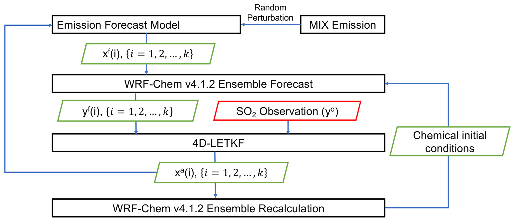
Figure 2Flow chart of the WRF-Chem/4D-LETKF SO2 emission inversion system by assimilating the SO2 observations.
As shown in Fig. 2, each assimilation cycle with 4D-LETKF includes two steps: a first guess and a state analysis. In our implementation, the first guess is the WRF-Chem ensemble forecasting for 12 h with hourly model output. The state analysis optimizes the SO2 emissions in the past 12 h. The advantages of 4D-LETKF used here are threefold: (1) each member of the ensemble WRF-Chem simulations is continuously integrated for 12 h; therefore, this avoids frequent switching between the ensemble WRF-Chem forecasts and the assimilation (Peng et al., 2017; D. Chen et al., 2019). (2) The asynchronous observations can be assimilated to optimize the current state (Hunt et al., 2007; Dai et al., 2019b). (3) The assimilation time window of 12 h could avoid filter convergence and divergence by finite ensemble samples, since more frequent assimilation forces the experiments more closer together, inducing the underestimation of the model spread and overconfidence in the first-guess state estimate (Schutgens et al., 2010; Miyazaki et al., 2012a; Hunt et al., 2007).
2.4 State variable and forecast model for emission
In this study, the state variable to be optimized is the SO2 emission. A forecast model for emission is required to propagate observation information and determine the first guess for the next assimilation cycle (Miyazaki et al., 2012a). We adopt the same forecast model for SO2 emission proposed by D. Chen et al. (2019). The forecast model for SO2 emission weights 75 % and 25 % toward the SO2 emission ensemble from the previous analysis and the static initial prior ensemble as in the following formula:
where M is the identity matrix. The optimized SO2 emission ensemble has SO2 emissions at 12-hourly time slots, which are used to calculate the first-guess SO2 emission ensemble in sequence for the next assimilation cycle. The SO2 emission inversion depends on the forecast model; therefore, sensitivity experiments for various different emission forecasts are conducted to tune the assimilation system as given in Table 1. The detailed settings of the sensitivity experiments will be described in the next section. As shown in Figs. S1 and S2 in the Supplement, the temporal and spatial distributions of the ensemble spread of the forecast emissions are significantly sensitive to the assimilation system parameters. The initial prior ensemble of SO2 emission is generated by perturbing the freely available MIX Asian inventory S for November 2010 (M. Li et al., 2017). For example, the SO2 emission for ensemble member i at a given location (x,y) is calculated as (Rubin et al., 2016), and the perturbation fi(x,y), {i=1, 2, …, k}, follows a log-normal distribution in the k-dimensional space. The mean and the variance of the perturbations f(x,y) are equal to 1 and the MIX SO2 uncertainty (i.e. 35 %) (M. Li et al., 2017). The horizontal perfectly correlated and random uncorrelated perturbations are both created to generate the initial prior ensemble and the associated first-guess SO2 emission ensemble as described later. The spatial distribution of the ensemble spread of the with either horizontal perfectly correlated or random uncorrelated perturbations has a similar pattern to the MIX Asian inventory S, which is generally equal to 35 % multiplied by S. In the MIX inventory, anthropogenic emissions are aggregated into five sectors: power, industry, residential, transportation, and agriculture. However, only the combined total emission is used in the model and updated in the analysis. This aims to decrease the degree of freedom in the analysis (Miyazaki et al., 2012a). A total of 10 chemical species including both gaseous and aerosol species are included in the MIX inventory (M. Li et al., 2017). The original monthly MIX anthropogenic emissions with a horizontal resolution of are remapped to the model resolution of 50 km. The residential, transportation, and agriculture emissions are allocated in the lowest model layer, whereas the power and industry emissions are allocated in the lowest seven model layers with the vertical profiles of the emission factors from the Model Inter-Comparison Study for Asia (MICS-Asia) phase III (L. Chen et al., 2019). An improved speciation framework for mapping Asian anthropogenic emissions of non-methane volatile organic compounds (NMVOCs) to multiple chemical mechanisms (Li et al., 2014) is adopted to prepare the initial hourly anthropogenic emissions every 12 h with two separated emission files (i.e. io_style_emissions = 2). We do not apply any diurnal variation for the MIX emissions. Therefore, the initial a priori emissions are identical throughout the 24 h. The emissions of aerosol species for WRF-Chem are prepared according to the study of Peng et al. (2017). Notably, only the SO2 emission is perturbed and optimized by CNEMC SO2 observations in this study.
The chemical initial conditions (i.e. atmospheric SO2 concentrations) for the next forward simulation of the WRF-Chem ensemble also need to be updated with the optimal emission ensemble from the previous analysis (Peng et al., 2015; Peters et al., 2005), and this is achieved by recalculation of the WRF-Chem ensemble with the optimized emissions (Fig. 2). In other words, the WRF-Chem ensemble is performed twice in one assimilation cycle. Theoretically, the uncertainties of the forecast SO2 concentrations by recalculation of the WRF-Chem ensemble are dependent on the optimized emissions. Lower uncertainties of the initial SO2 conditions for the next assimilation cycle should be found with higher accurate optimized SO2 emissions, which in turn makes the SO2 emission inversion more reasonable. Sensitivity experiments for the SO2 emission inversions as described in the next section are performed to choose the best assimilation system parameters.
The effectiveness of 4D-LETKF is highly dependent on having sufficient spread in the ensemble members in order for the observations to impact the first guess (Rubin et al., 2016; Dai et al., 2019b; Hunt et al., 2007). The ensembles represent the uncertainty in the model first guess; therefore, the method for generating the ensemble is an important consideration for an optimal top-down emission inversion. Meanwhile, 4D-LETKF allows a flexible choice of observations to be assimilated for a specific grid point through horizontal, vertical, and temporal observation localizations (Miyoshi et al., 2007; Dai et al., 2019b; Cheng et al., 2019). The observation localization gradually reduces the effect of an observation as the increasing departure from the analysis grid. In this study, the horizontal localization factor is calculated as the Gaussian function (Miyoshi et al., 2007):
where σ is the localization length, and r is defined as the physical distance between the observation and the analysis grid, and we force the localization factor to zero at 3.65 times the localization length (Zhao et al., 2015). In other words, we ignore observations beyond the cut-off distance. The tuneable horizontal and temporal localization lengths are defined in physical distance (km) and time (h), respectively. The vertical localization is not applied for the SO2 emission inversion in this study. In other words, we trust the vertical profiles of the emission factors from the Model Inter-Comparison Study for Asia (MICS-Asia) phase III (L. Chen et al., 2019).
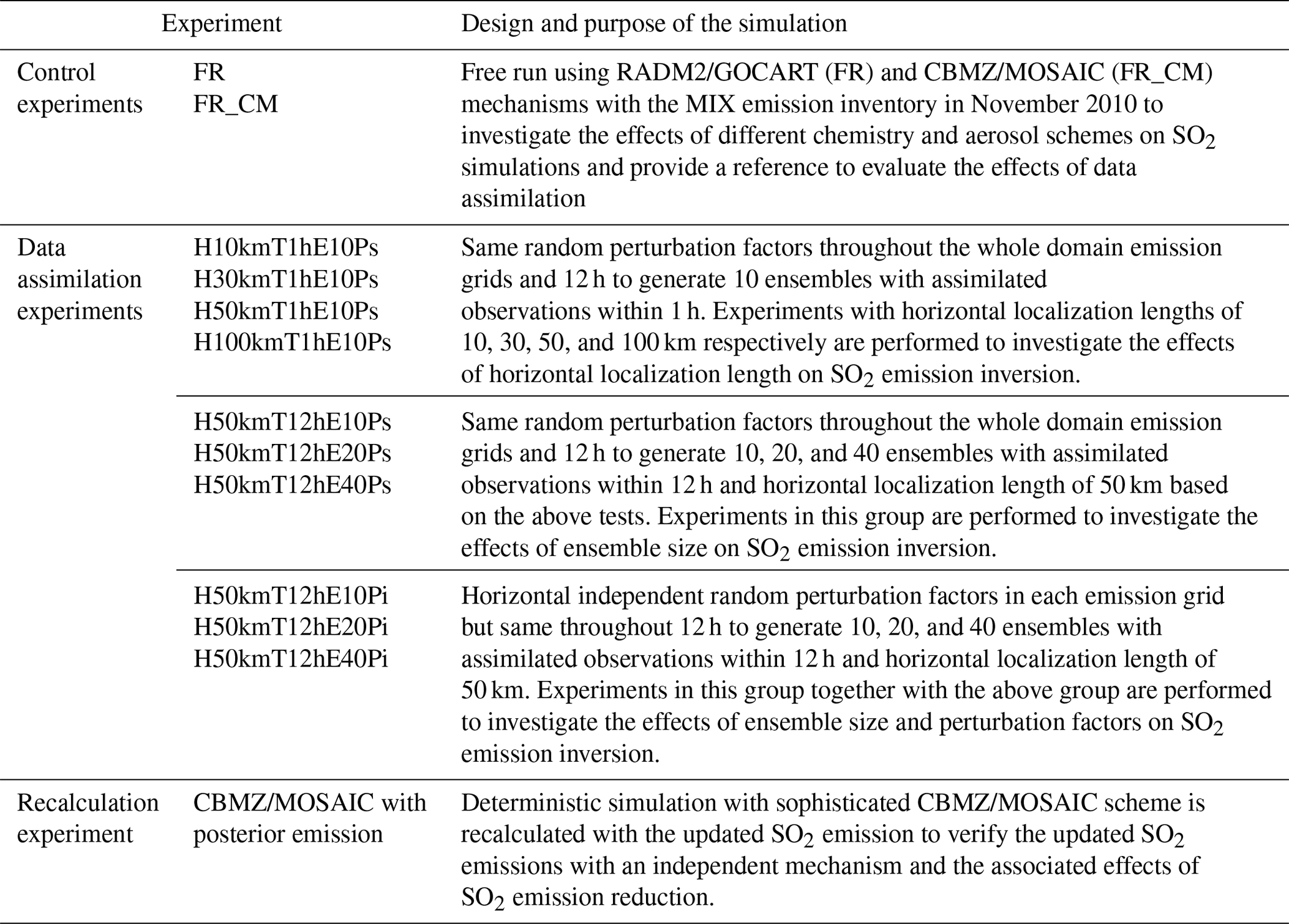
A correct choice of the assimilation system parameters such as the ensemble size and correlation length is important to improve the data assimilation performance (Miyazaki et al., 2012b). A series of sensitivity experiments are performed to tune the assimilation system as listed in Table 1. A control experiment assuming the same emissions in November 2016 as in November 2010 (i.e. the standard MIX emissions) is conducted as the deterministic simulation to assess the influence of data assimilation. Considering the GOCART aerosol scheme uses a simple representation of the aerosol chemistry for reducing the computational load, we also conduct another deterministic simulation using a more sophisticated aerosol chemical scheme named Model for Simulating Aerosol Interactions and Chemistry (MOSAIC), coupled with the “lumped-structure” Carbon Bond Mechanism (CBMZ) (Zaveri et al., 2008) (i.e. chem_opt = 9) to investigate the effects of different chemistry and aerosol schemes on SO2 oxidation. The data assimilation experiments are divided into three groups. In the first group, the same random perturbation factor throughout the whole domain emission grids including vertical and temporal spaces per member is applied to the MIX SO2 emission to generate 10 ensemble members for the WRF-Chem ensemble forward simulation. The spatial correlation coefficients among the initial prior ensemble of SO2 emissions over every two model grids are equal to 1, and this makes the spatial correlations among the grid points of the forecast emissions also equal to 1. The same random perturbation factor generates a perfect correlation of emission in both the spatial and temporal spaces; however, this should not be seen as overly restrictive (Schutgens et al., 2010). Firstly, the bottom-up SO2 emission inventories are to a large extent based on the used activity rates and emission factors (Li et al., 2018). Therefore, with the same random perturbation factors, we effectively create an ensemble of inventories derived with different activity rates and emission factors. Secondly, the same emission standards for SO2 emission mitigation are implemented in China (Zheng et al., 2018), and this causes the SO2 reductions to be correlated to a certain extent in both spatial and temporal spaces. Thirdly, the analysis is conducted locally in 4D-LETKF, and the analysis at two grids separated by a distance over about 7.3 times the localization length is mostly independent (Schutgens et al., 2010). In this group, the strongest temporal localization is applied to assimilate only the observations within 1 h of the analysis time. In other words, the hourly SO2 emission is optimized using only the CNEMC SO2 observation within the subsequent 1 h, making the inverted SO2 emission variable hour by hour. The difference of the experiments in this group is only the horizontal localization length, which is assumed to be 10, 30, 50, and 100 km respectively. The purpose of the experiments in this group is to investigate the effects of horizontal localization length on SO2 emission inversion. Based on the results in the first group as described later in Sect. 4, the second group of experiments by fixing the horizontal localization length of 50 km is subsequently performed with 10, 20, and 40 ensemble members to investigate the effects of ensemble size on SO2 assimilation. In this group, we remove the temporal localization to investigate the effects of temporal localization on the SO2 emission inversion. In other words, the hourly SO2 emission is optimized using all the CNEMC SO2 observations within the 12 h assimilation window, making the inverted SO2 emission constant within every 12 h. In the third group, the experiments are performed the same as those of the second group except that the ensembles are generated by independently perturbing the emission in horizontal space but dependently in vertical and temporal spaces. These last two groups of experiments are used to investigate the effects of the ensemble size and perturbation factor on SO2 emission inversion. The sensitivity data assimilation experiments are all performed for 10 d over the period of 00:00 UTC 8 November to 00:00 UTC 18 November 2016. The global model MOZART-4/GEOS-5 provides the initial and lateral boundary conditions used in this study (https://www.acom.ucar.edu/wrf-chem/mozart.shtml, last access: 10 August 2020). Since we do not know the uncertainties of the global model MOZART-4/GEOS-5, the initial and lateral boundary chemical fields are not perturbed in this study. The first 3 d is used as the spin-up of the data assimilation system, and the subsequent simulation results for 1 week are analysed in the next section. Based on the sensitivity tests of the SO2 emission inversion system, the experiment H50kmT1hE10Ps, which generally performed better than other experiments, is extended to 00:00 UTC on 1 December 2016. This provides a longer period of 20 d to further validate the assimilation system. We also perform a recalculation experiment with the sophisticated CBMZ/MOSAIC scheme and the updated SO2 emissions to verify the new SO2 emission and the associated effects of SO2 emission reduction.
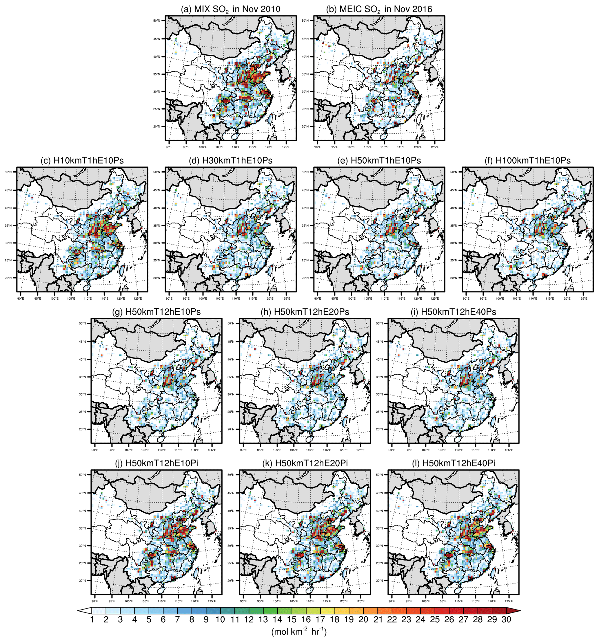
Figure 3Spatial distributions of the MIX SO2 emission in November 2010 (a) and the MEIC SO2 emission in November 2016 (b) in the model's lowest layer. Spatial distributions of the inverted SO2 emissions in November 2016 in various data assimilation experiments (c–l).
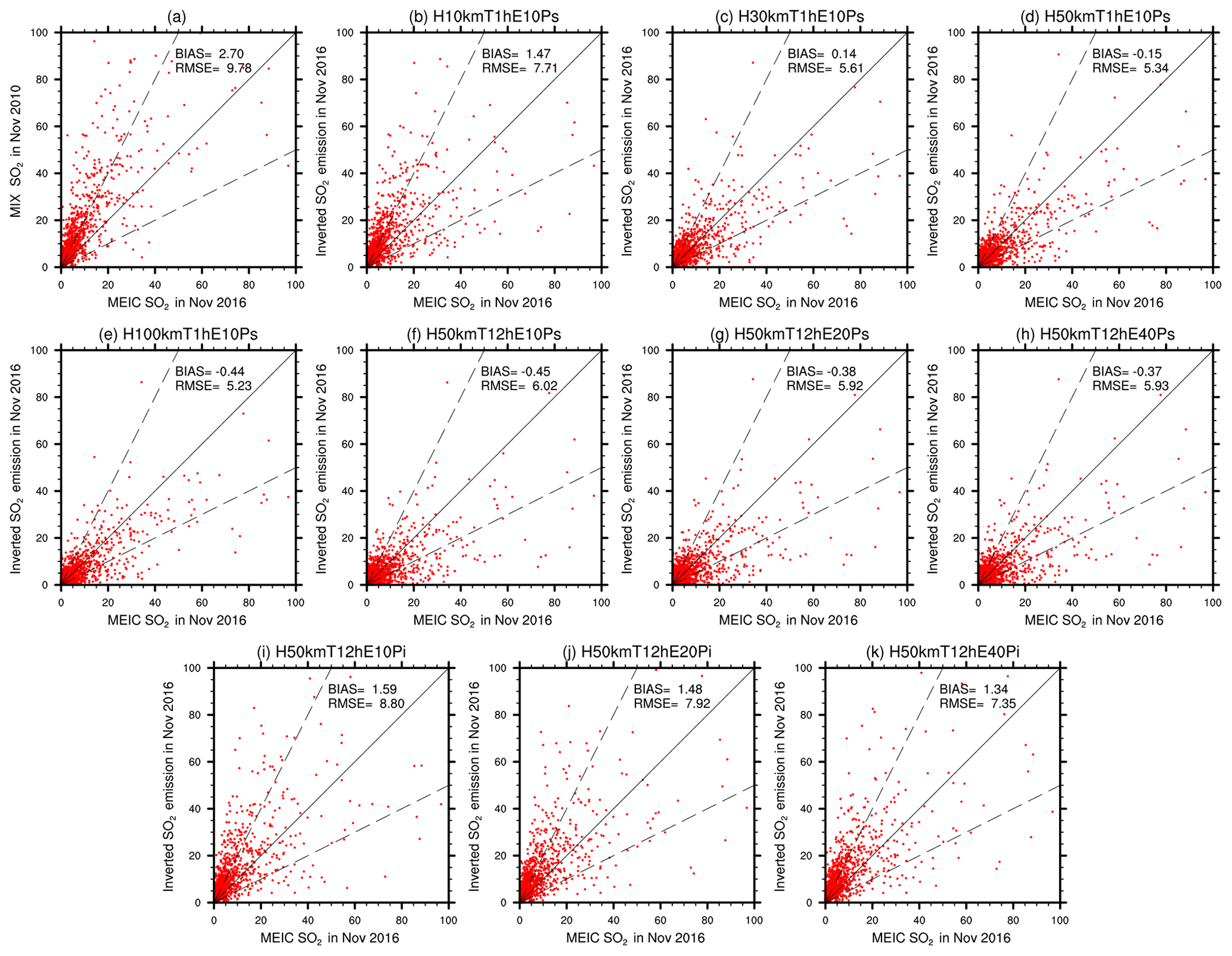
Figure 4Comparisons of the MIX SO2 emissions in November 2010 (a) and the inverted SO2 emission in November 2016 in various data assimilation experiments (b–k) to the MEIC SO2 emissions in November 2016.
4.1 Sensitivity of the inverted SO2 emission to the assimilation parameters
The spatial distribution of the MIX SO2 emission in November 2010 at the model lowest layer is shown in Fig. 3a, which serves as the base of the initial a priori SO2 emission for our experiments in November 2016. The hotspots of anthropogenic SO2 emission are found over the economically developed areas such as the North China Plain (NCP), the Yangtze River Delta (YRD), and the Pearl River Delta (PRD). The Multi-resolution Emission Inventory for China (MEIC; http://www.meicmodel.org, last access: 15 February 2021) developed by Tsinghua University can provide the updated SO2 emission for November 2016 (Fig. 3b), which is used as the independent bottom-up SO2 emission to validate our inverted SO2 emission. It is apparent that significant negative changes of SO2 emission are found over the a priori higher source regions such as the NCP, YRD, and PRD between the years 2010 and 2016, which is in agreement with the changes of the column SO2 concentrations observed by satellites (Wang et al., 2018). As a consequence of the clean air actions (Zheng et al., 2018), the SO2 emissions over most areas of China showed a systematic decline from the year 2010 to 2016 (Fig. 4a). Can we reveal the reductions of the SO2 emission by assimilating the CNEMC-observed surface SO2 concentration?
As shown in Figs. 3c–f and 4b–e, both spatial distribution and magnitude of the inverted SO2 emission in November 2016 firstly become closer to the independent MEIC ones but get worse subsequently as the horizontal localization length of the assimilation system increases. The inverted SO2 emissions of each assimilation experiment are obtained by averaging the ones over the ensemble members. The spatial distributions of the mean differences of the MIX and inverted SO2 emissions minus the MEIC ones are shown in Fig. S3, and the spatial distributions of the mean ratios between the inverted SO2 emissions and the MIX ones are shown in Fig. S4. The time series of the hourly SO2 emissions averaged over China of the initial MIX prior, the forecast, and the analysis of the assimilation experiment H50kmT1hE10Ps from 00:00 UTC 8 November to 23:00 UTC 17 November 2016 are also shown in Fig. S5, which illustrates the adjustment of SO2 emissions with data assimilation. The experiment with the smallest horizontal localization length (i.e. 10 km) only optimizes the SO2 emission over the specific grids where there are observations to be assimilated. In such a case, the significant reductions of the SO2 emission over the grids with no observation sites are unable to be revealed, such as Shandong province in the NCP. With a larger localization length, an observation can constrain the emissions in more grids surrounding the observation, and the observation error more gently increases as the distance from the observation location increases (Hunt et al., 2007). It is obvious that the systemic SO2 emission reductions especially over the Shandong province are detected by increasing the horizontal localization length. However, the perfect correlations of the emission perturbations over the domains with too large a horizontal localization length cause spurious error covariance, causing the more local emission changes to be undetectable. This is demonstrated by the inverted SO2 emissions with a localization length of 100 km tending to be lower than the independent MEIC ones, with a mean bias of −0.44 mol km−2 h−1. Generally speaking, the inverted SO2 emissions with a horizontal localization length of 50 km are best in agreement with the MEIC ones, with a mean bias of −0.15 mol km−2 h−1 and root mean square error (RMSE) of 5.34 mol km−2 h−1.
With a horizontal localization length of 50 km, the spatial distribution of the inverted SO2 emission by removing the temporal localization is shown in Fig. 3g. It is clearly found that the inverted SO2 emissions over the Shandong province, YRD, and PRD without temporal localization are lower than those with temporal localization, inducing a larger negative bias and RMSE (Fig. 4f). This demonstrates that it is important to reveal the diurnal variations of the SO2 emission (Wang et al., 2010). The experiment with temporal localization can reveal the hourly variation of the SO2 emission by assimilating only the subsequent hourly observations, whereas the experiment without temporal localization only adjusts the magnitude of SO2 emission every 12 h by assimilating all the observations within the 12 h window.
As shown in Figs. 3g–i and 4f–h, there are no significant differences of the horizontal distribution and magnitude of the inverted SO2 emission between 10, 20, and 40 ensemble members. This indicates that the ensemble size has little effect on the SO2 emission inversion when randomly correlated perturbing the emissions. The ensemble forecast with 10 members seems feasible to reveal the SO2 reductions in China, although the inverted emissions have not converged properly. This in turn significantly reduces the required computational resources and time for the forward calculation of the ensemble model, making the dynamical update of air pollutant emissions affordable when assimilating near-real-time observations.
The inverted SO2 emission with horizontal random uncorrelated perturbations becomes closer to the independent MEIC one as the number of the ensemble members is increased (Figs. 3j–l and 4i–k). However, the performances of the horizontal distribution and magnitude of the inverted SO2 emission using 40 ensemble members with horizontal random uncorrelated perturbations are clearly even worse than those using 10 ensemble members with horizontal correlated perturbations. This demonstrates that the independent emission perturbations over each model grid tend to underestimate the model spread due to the current limited ensemble members and the cancellation of neighbouring cells (Pagowski and Grell, 2012; Schutgens et al., 2010).
The mean bias and RMSE of SO2 emission over China using the MIX SO2 emission in November 2010 for November 2016 are 2.70 and 9.78 mol km−2 h−1, respectively (Fig. 4a). For the inverted SO2 emission by data assimilation, the bias and RMSE reduction rates (Miyazaki et al., 2012b) are estimated as follows:
where BDA and RMSEDA are the mean bias and RMSE between the inverted SO2 emission and the MEIC SO2 emission in November 2016. As shown in Fig. 5, it is found that (1) the inverted SO2 emission in every assimilation experiment can reduce both the bias and the RMSE; (2) the randomly correlated perturbation factor is superior to the randomly uncorrelated perturbation factor in reducing the bias and RMSE, and it is generally unaffected by the ensemble size; (3) the experiment H50kmT1hE10Ps shows the best performance in reducing both the bias and the RMSE, decreasing the bias and RMSE by 94.5 % and 45.4 % respectively.
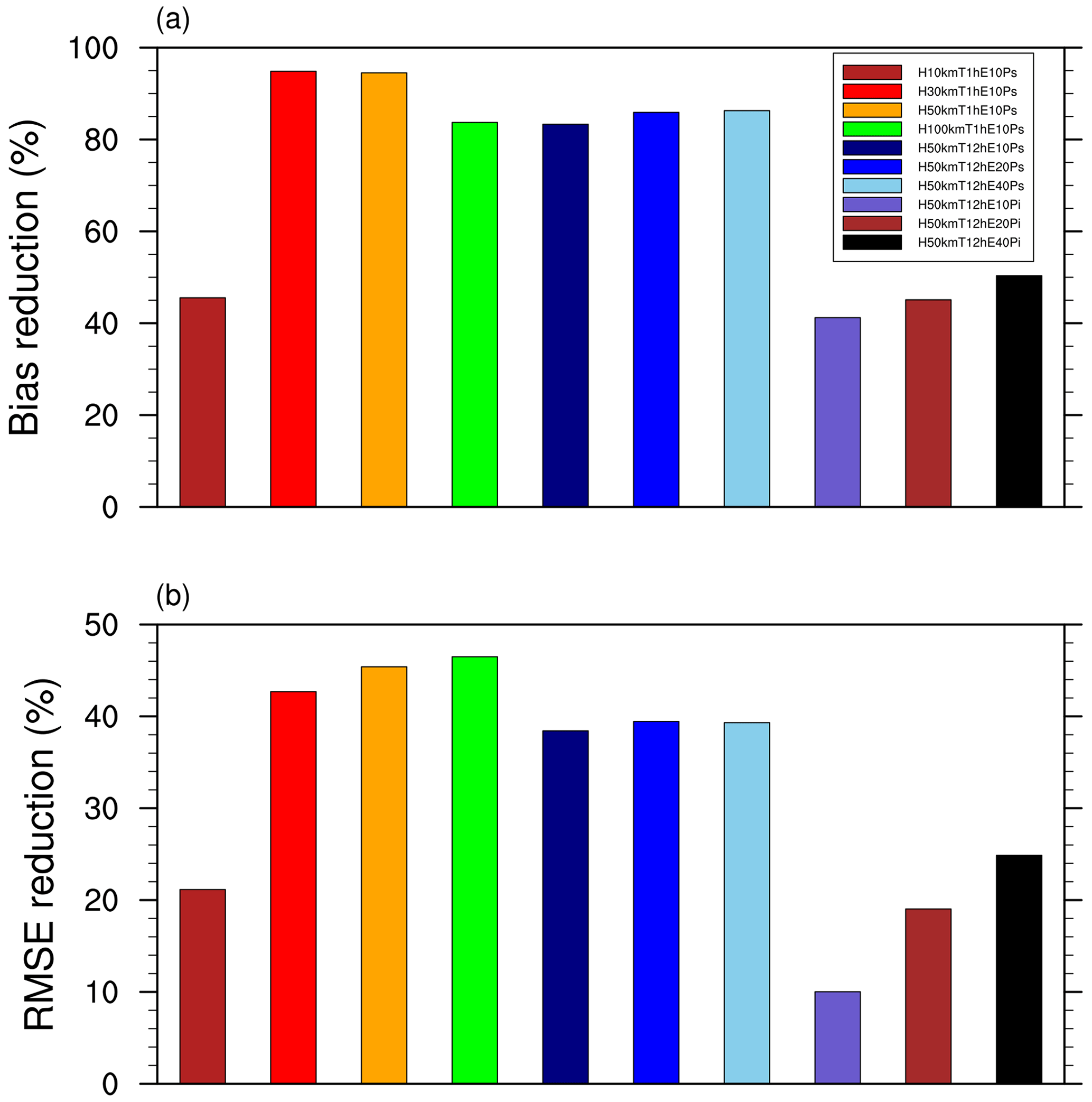
Figure 5Reductions of the bias and root mean square error (RMSE) between the inverted SO2 emissions in various data assimilation experiments and the MEIC ones referring to those between the MIX and MEIC SO2 emissions.
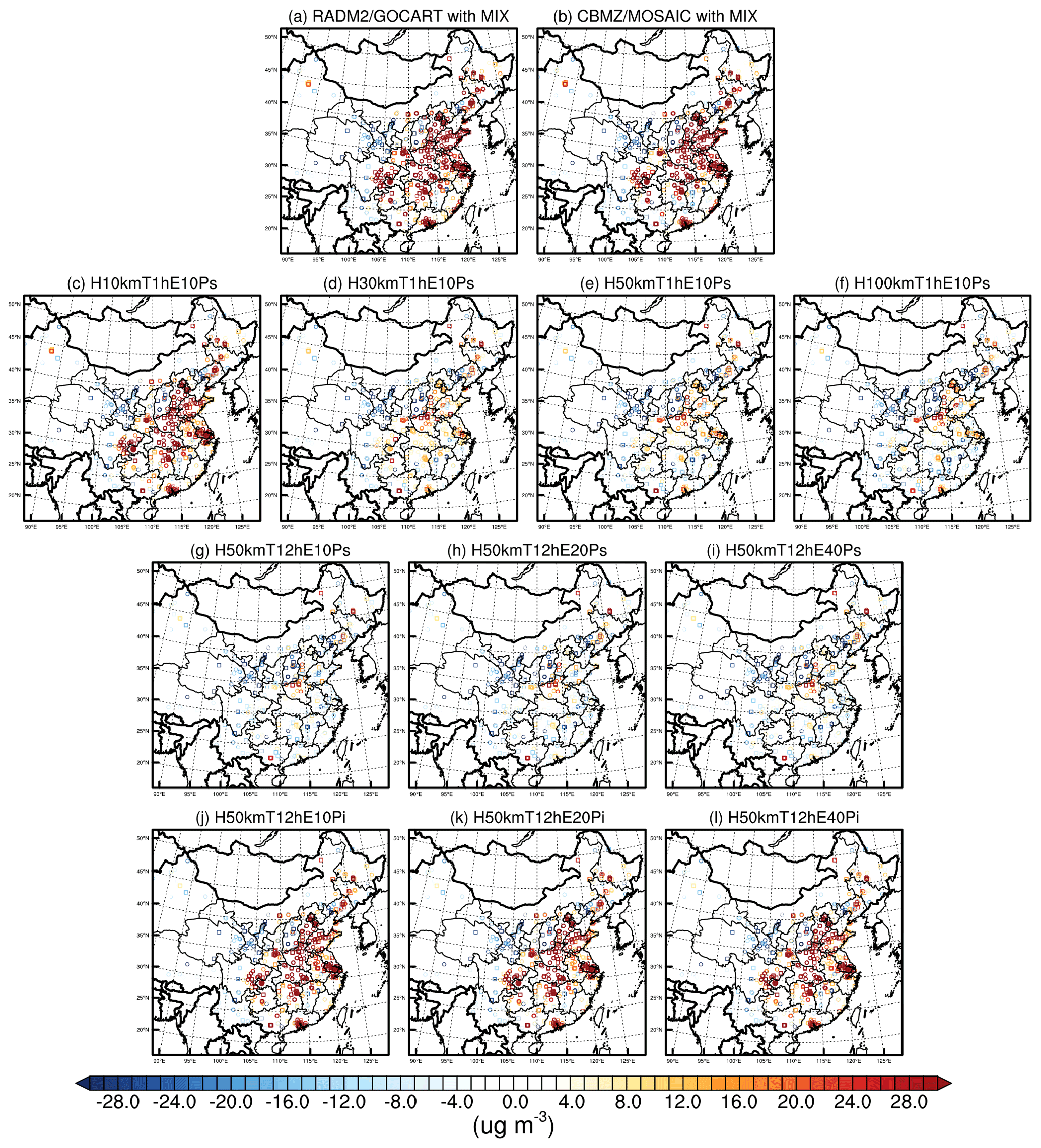
Figure 6Spatial distributions of the mean biases between the simulated surface SO2 concentrations in various experiments and the CNEMC-observed ones over both the assimilated and independent sites. The locations of the assimilated and independent verification observation sites of the CNEMC are shown by the circles and squares, respectively.
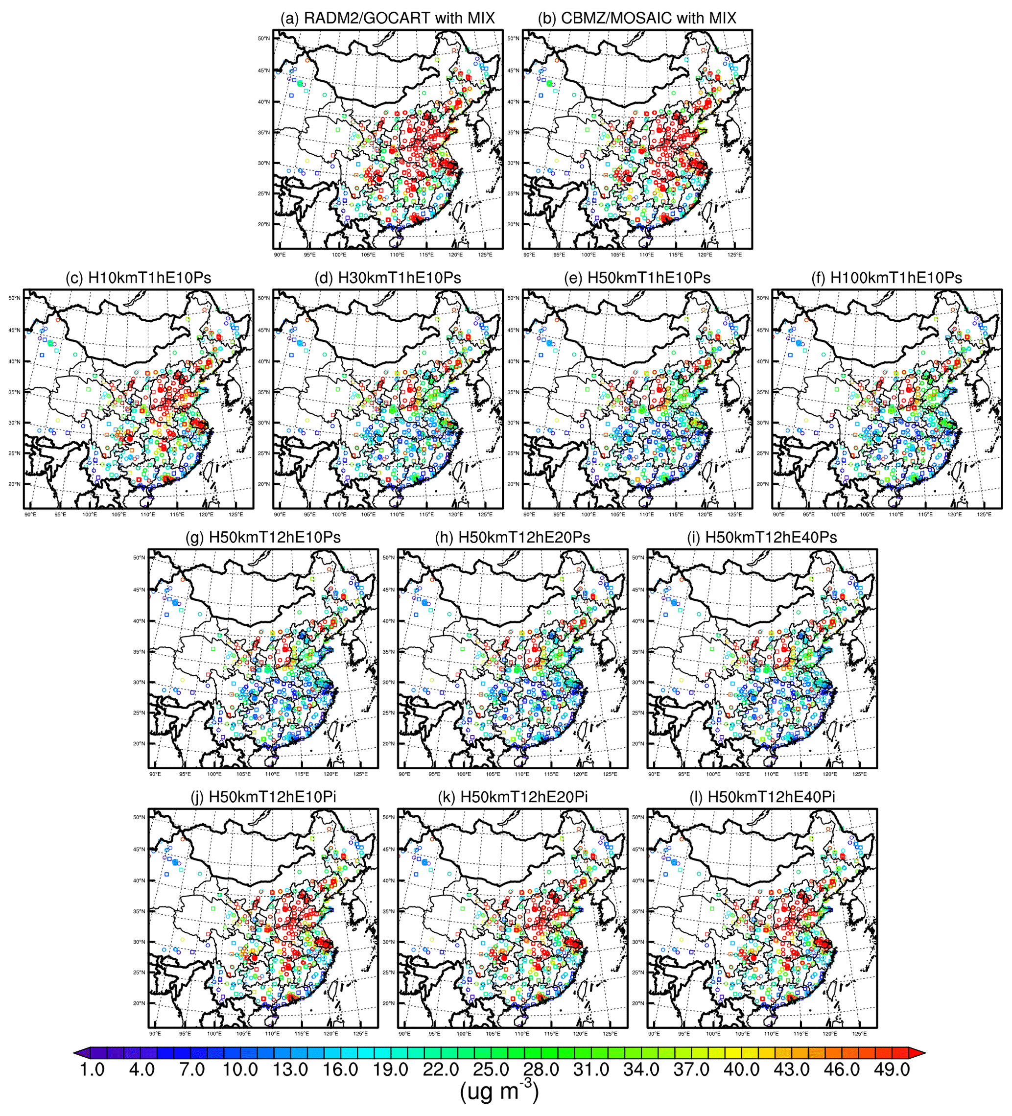
Figure 7Same as Fig. 6 but for the RMSEs.
4.2 Sensitivity of the surface SO2 concentration to the emission
Figures 6 and 7 show the horizontal distributions of the biases and RMSEs between the surface SO2 concentrations simulated in various experiments and the CNEMC-observed ones over both the assimilated and independent sites. The SO2 concentrations in each assimilation experiment are obtained by averaging the ones over the WRF-Chem ensemble recalculations with the optimized emissions. The spatial distributions of the mean SO2 concentrations simulated with the original MIX emissions and the updates of the simulated SO2 concentrations with the inverted SO2 emissions are shown in Fig. S6. The spatial distributions of the mean differences of the SO2 concentrations simulated in the FR and FR_CM experiments are also shown in Fig. S6. It is apparent that significant RMSEs and positive biases are found over the a priori SO2 emission hotspot regions such as the NCP, YRD, and PRD in both the two free-run experiments, whereas slight RMSEs and negative biases are both found over northwestern China. Furthermore, the horizontal distributions of both the biases and RMSEs of the two free-run experiments are generally similar. As given in Table 2, the relative differences of the RMSEs in the FR and FR_CM experiments are both less than 1 % over the assimilated and independent sites, although the mean biases in the FR_CM experiment both tend to be slightly smaller than those in the FR experiment. This demonstrates that the biases and RMSEs between the simulated and observed surface SO2 concentrations are not induced by the uncertainties of the different chemical reaction mechanisms but are due to the uncertainties of the used SO2 emissions. The simulated ensemble mean surface SO2 concentrations by recalculating the WRF-Chem with the inverted SO2 emissions in all assimilation experiments are shown to be more comparable to the observations, and the performances of the simulated SO2 surface concentrations are clearly affected by the inputs of the different inverted SO2 emissions due to assimilation system parameters. This indicates that the uncertainties of the different chemical reaction mechanisms in simulating SO2 concentrations are much smaller than those of the SO2 emissions. In the first group of data assimilation experiments, the largest biases and RMSEs of the simulated and observed SO2 surface concentrations over both the assimilated and independent sites are found in the H10kmT1hE10Ps experiment. This indicates that the SO2 emission changes existing grid correlations, and the SO2 emission inversions over only the grids with available assimilated sites are not sufficient to reveal the real SO2 emission changes in the grids without observation sites. In addition, the largest biases and RMSEs over both the assimilated and independent sites are still found in the third group of data assimilation experiments, although the biases and RMSEs decrease with the increase of the number of ensemble members. This further illustrates there are correlations of the gridded SO2 emission changes, and the random perfectly correlated emission perturbation factors over the model grids are superior to the random uncorrelated emission perturbations for current emission inversions. The latter is probably due to the currently limited number of ensemble members for reducing the computational resources. However, the sophisticated random uncorrelated emission perturbations should have better performances with large or unlimited ensemble members. Similar to the inverted emissions, the experiments in the second group show the ensemble size has little effect on the biases and RMSEs of the SO2 surface concentrations over both the assimilated and independent sites when the ensemble members are generated by perturbing the emissions perfectly correlated over the domain grids. The reductions of the biases of the SO2 surface concentrations in both the assimilated and independent sites benefit from the temporal localization, although the RMSEs are slightly increased. It is interesting that the smallest RMSE of the SO2 surface concentrations over the independent sites is also found in the H50kmT1hE10Ps experiment, with a value of 36.20, which shows that the inverted SO2 emissions are also best in agreement with the independent MEIC ones. This further indicates that the assimilation system parameters used in this experiment are suitable for the SO2 emission inversion, decreasing the biases of SO2 surface concentrations over assimilated and independent sites by 87.2 % and 88.9 % respectively. The underestimation of the surface SO2 concentration with the original MIX emission over northwestern China such as the Gansu province is potentially attributable to the increasing SO2 emissions due to energy industry expansion and relocation over northwestern China (Ling et al., 2017). The SO2 emissions and surface concentrations over the Gansu province are increased to reduce the negative biases in the assimilation experiments as shown in Figs. S4 and S6, indicating that our emission inversion system also works well when the prior emissions are underestimated. However, the simulated surface SO2 concentrations with the inverted emissions are still underestimated over the Gansu province. The reason for the underestimation is twofold: (1) there are limited observations to be assimilated over northwestern China because the observation sites are sparse; (2) the initial a priori MIX SO2 emission over northwestern China is small and underestimated, causing the model uncertainty to be small relative to the observation one. This translates to a reduced impact of the observation on the a priori emission.
Table 2The mean biases and root mean square errors (RMSEs) of the simulated SO2 surface concentrations in various experiments and the CNEMC-observed ones over all assimilated and independent sites.
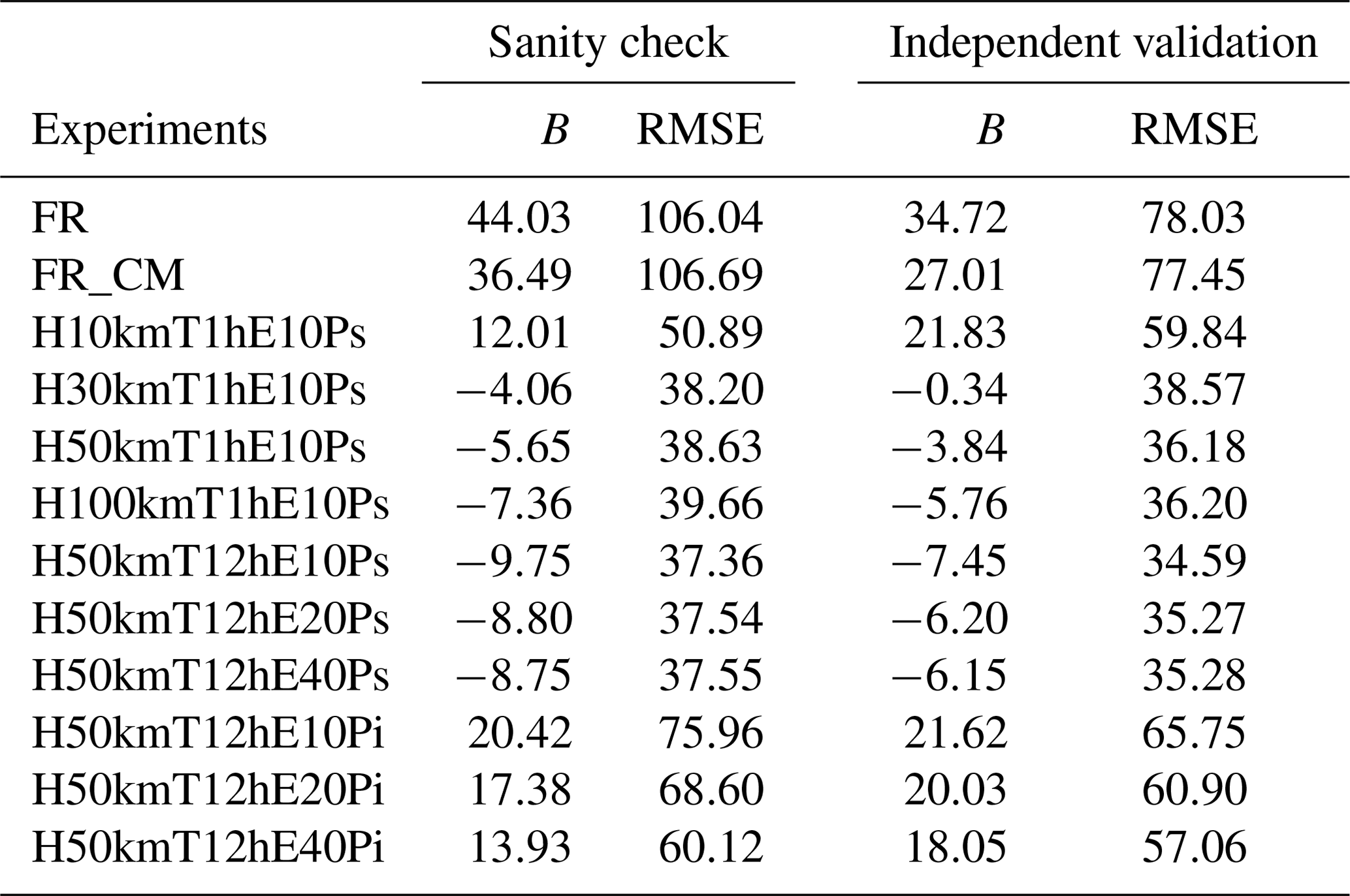
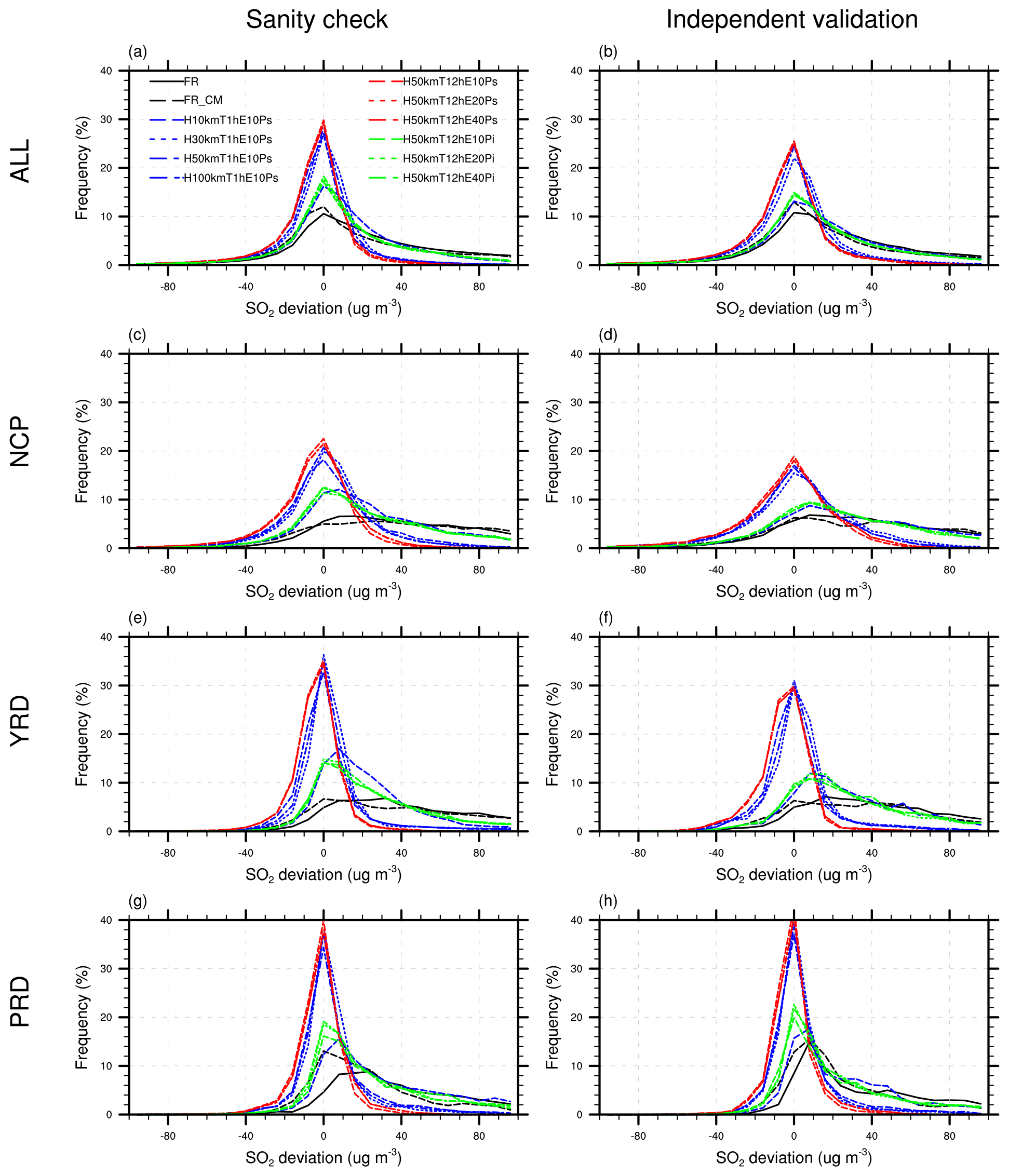
Figure 8Frequency distributions of the deviations of the simulated SO2 surface concentrations in various experiments minus the observed ones.
Figure 8 illustrates the frequency distributions of the deviations of the simulated SO2 surface concentrations in various experiments minus the observed ones. It is expected that the distributions of the SO2 surface concentrations deviations for the two free-run experiments in China and the three subregions are all positively biased due to the known overestimation of the SO2 emissions. The distributions of the SO2 surface concentration deviations with the updated SO2 emissions in all the data assimilation experiments show reduced biases over both the assimilated and independent sites. However, the distributions of the deviations with the updated SO2 emissions in the third group of experiments and the H10kmT1hE10Ps experiment are still positively biased, whereas slightly negative biased distributions are found in the second group of experiments and the H100kmT1hE10Ps experiment. The distributions of the SO2 concentration deviations with the updated SO2 emissions in the H50kmT1hE10Ps experiment, as expected, show the best performance, with a peak closer to 0 in both the assimilated and independent sites.
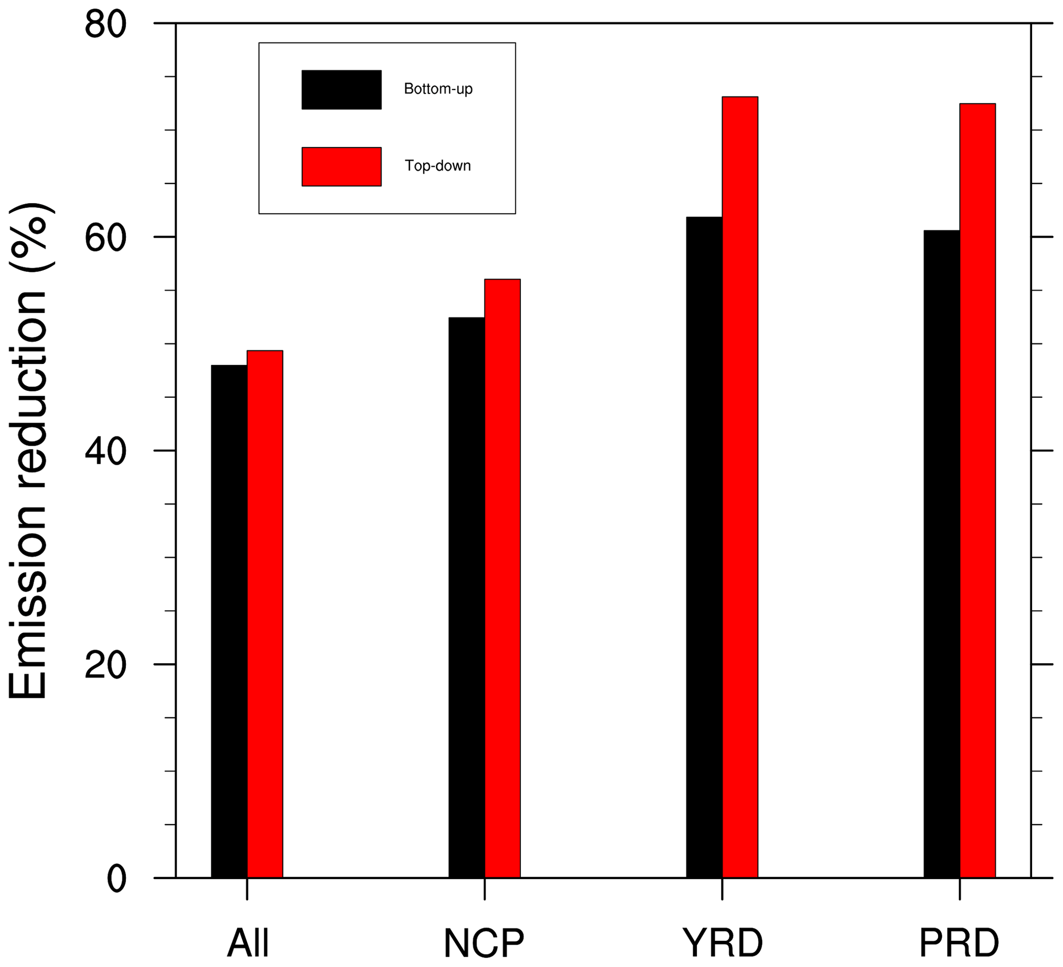
Figure 9SO2 emission reductions in November over the period 2010 to 2016 in China and the three subregions estimated by the bottom-up and top-down approaches.
4.3 SO2 reduction in China and associated effects
Based on the aforementioned sensitivity tests of the SO2 emission inversion system, the experiment H50kmT1hE10Ps is extended to 00:00 UTC on 1 December 2016. This provides a longer period for 20 d to estimate the reduction of the SO2 emission over China in November over the period 2010–2016. The bottom-up and top-down estimations of the SO2 emission reduction from 2010 to 2016 are calculated by comparing the MEIC and inverted SO2 emissions by data assimilation in November 2016 to the MIX SO2 emission in November 2010. As shown in Fig. 9, the top-down estimation of the SO2 emission reduction over China is 49.4 %, which is well in agreement with the bottom-up estimation of 48.0 %. In addition, larger SO2 emission reductions over the three subregions estimated by the bottom-up approach are correctly revealed by the emission inversion system. The top-down and bottom-up estimations of the SO2 emission reduction over NCP are generally comparable, with values of 56.0% and 52.4 % respectively. The largest SO2 emission reductions both with the top-down and bottom-up approaches are found over the YRD region, with values of 73.1 % and 61.8 % respectively. The SO2 emission reduction using the top-down approach is 10 % higher than that using the bottom-up approach over the PRD region. To validate the inverted SO2 emissions and explore the possible reasons of the overestimation of SO2 emission reduction over the YRD and PRD using the top-down approach, the time series of the simulated SO2 surface concentrations in various experiments and the observed ones are shown in Fig. 10. The simulated SO2 surface concentrations, especially over the YRD subregion in the two free-run experiments, show significant positive biases over all the period, revealing the drawback of the prescribed SO2 emissions in November 2016 being the same as in November 2010. The simulated SO2 surface concentrations with the inverted SO2 emissions using both the RADM2/GOCART and CBMZ/MOSAIC chemical reaction mechanisms are much closer to the observations in both the assimilated and independent sites over all the period. This demonstrates that the WRF-Chem/4D-LETKF emission inversion system can continuously and dynamically update the SO2 emissions by assimilating the newly available observations as shown Fig. S5. The SO2 surface concentrations simulated by the FR_CM experiment are sometime lower than those in the FR experiment, especially over the YRD and PRD subregions, indicating the overestimations of the SO2 emission reduction using the top-down approach over the YRD and PRD are probably due to the simple aerosol chemistry schemes used in RADM2/GOCART (Chin et al., 2000). This is proved as the simulated SO2 surface concentrations in YRD with the RADM2/GOCART scheme and the inverted SO2 emissions over the period 18–22 November 2016 are generally comparable to the observed ones, whereas the simulated SO2 surface concentrations with the sophisticated CBMZ/MOSAIC scheme and the inverted SO2 emissions are lower than the observed ones. The simulated SO2 surface concentrations at all sites with the inverted emission in both the FR_CM and assimilation recalculation are generally underestimated. This is due to the inverted emission being sufficient to reduce the overestimations of SO2 concentration over the a priori SO2 emission hotspot regions but insufficient to eliminate the underestimations over northwestern China.

Figure 10Time series of the simulated SO2 surface concentrations in various experiments and the CNEMC observations.
Based on the inverted SO2 emissions from 11 November to 1 December 2016, the daily and diurnal variations of the SO2 emission reductions over China and the NCP subregion are estimated as shown in Fig. 11a and b respectively, and the diurnal variations of the inverted SO2 emissions over China and the NCP subregion are also shown in Fig. 11c. Generally speaking, the daily variation of the SO2 emission reduction over China is not so significant. Larger SO2 emission reductions over the period 17 to 19 November in the NCP induced by the first orange alert for heavy winter air pollution in 2016 are clearly detected by the inverted emissions (Shi et al., 2019). Lower SO2 emission reductions over China and NCP from 21 to 22 November are probably contaminated by the strong cold wind from the northwestern direction, inducing the low SO2 concentrations and underestimating the associated ensemble spread. The latter causes the inverted emission to be overconfident in the background emission (Hunt et al., 2007). Since the emissions are constant over time in the a priori MIX inventory, the diurnal variations of the SO2 emission reduction over China and NCP both reveal higher emission reductions in the night-time, causing the SO2 emissions in the night-time to be lower than those in the daytime (Fig. 11c). This is generally reasonable as fewer human and economic activities happen in the night-time (L. Chen et al., 2019).
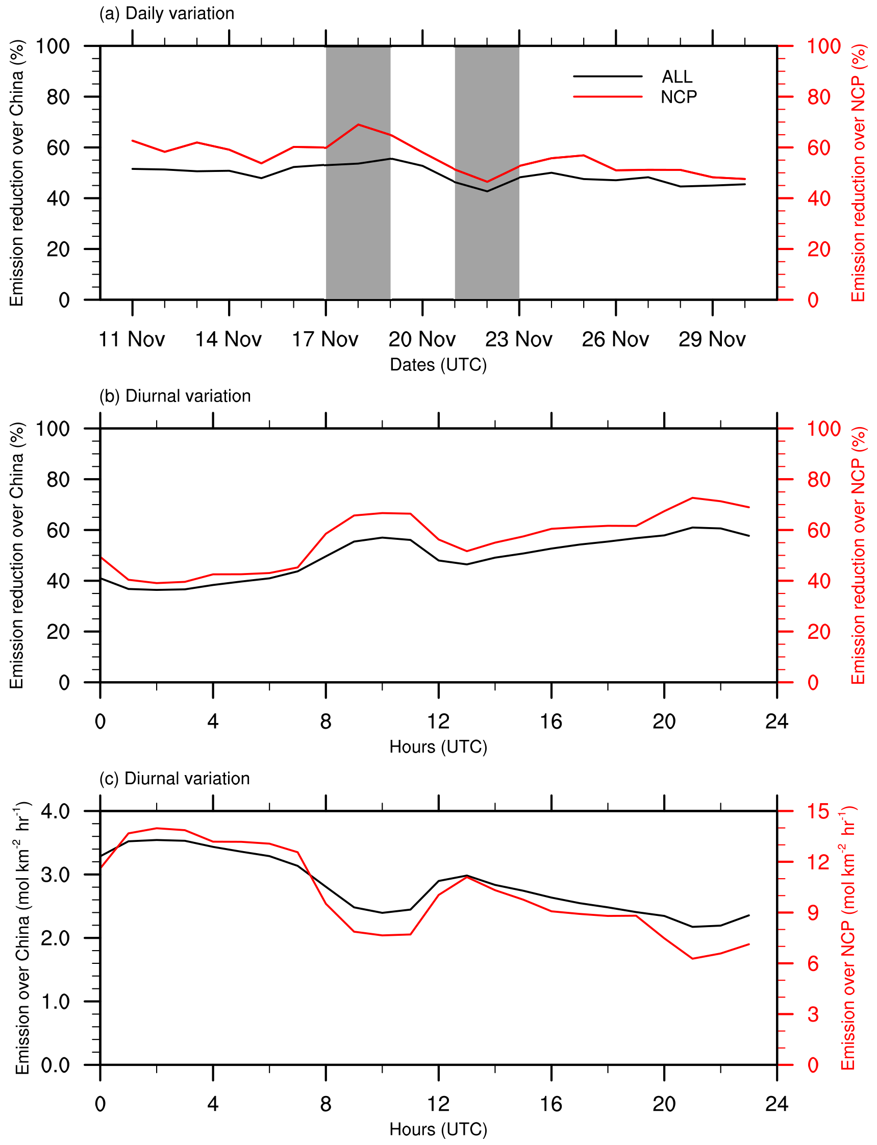
Figure 11Daily (a) and diurnal (b) variations of the SO2 emission reductions over China and the NCP subregion based on the inverted emissions. Diurnal variations of the inverted SO2 emissions over China and the NCP subregion (c).
Figure 12 shows the spatial distributions of the averaged surface concentrations of the sulfate, ammonium, nitrate, and PM2.5 over 11 November to 1 December 2016 simulated with the CBMZ/MOSAIC mechanism and the original MIX emissions and the absolute and relative changes of the associated aerosol surface concentrations with the newly inverted emissions by data assimilation. It is found that the SO2 emission reductions cause the sulfate surface concentrations to be reduced by up to 10 µg m−3 (50 % over central China), and this is due to the sulfate aerosols being dominated by the occurrence of in-cloud oxidation (Chin et al., 2000; Goto et al., 2015) and more clouds being found over central China (Li et al., 2015; Ma et al., 2014). The nitrate surface concentrations are found slightly increased in central China with the reduction of sulfate aerosols, and this is due to the emissions of the nitrate precursors (i.e. NO and NO2) not being updated in this study and because NH4NO3 is formed only in sulfate-poor aerosols (Zaveri et al., 2008; Chen et al., 2016). The synergy effects of sulfate–nitrate–ammonium induce slight reductions of ammonium surface concentrations, decreasing the PM2.5 surface concentrations by about 10 µg m−3 (10 %) over central China.

Figure 12Spatial distributions of the averaged surface concentrations of the sulfate, ammonium, nitrate, and PM2.5 over 11 November to 1 December 2016, simulated with the CBMZ/MOSAIC mechanism and the MIX emissions in November 2010, and the absolute and relative changes of the associated aerosol surface concentrations with the updated emissions by data assimilation.
Timely precise emission inventories are crucial to air quality prediction and mitigation. To dynamically update the emissions of air pollutants, we have developed a new emission inversion system based on the 4D-LETKF and the fully coupled model named WRF-Chem. Our emission inversion system considers the complex non-linear relationship between atmospheric chemical concentrations and emissions by ensemble forecasting with perturbed emissions. The emission inversion system is examined to update the outdated MIX SO2 emissions in November 2010 by assimilating the quality-assured and quality-controlled observations of SO2 surface concentration from the CNEMC in November 2016. The inverted SO2 emissions over China by data assimilation for November 2016 are validated with the independent MEIC emissions in November 2016.
Sensitivity tests for the emission inversion system demonstrate that the assumption of the covariance error matrix of the a priori SO2 emissions has the largest effect on the inverted emissions. The random perfectly correlated emission perturbations throughout the whole model grids with a horizontal localization length of 50 km can best reproduce the independent MEIC SO2 emissions, decreasing the MIX emission bias and RMSE by 94.5 % and 45.4 % respectively. The independent emission perturbations over each model grid tend to underestimate the model spread due to the currently limited number of ensemble members and the cancellation of neighbouring cells. With the random perfectly correlated emission perturbations, the ensemble size only has little effect on the inverted SO2 emissions, and the ensemble forecast with 10 members seems feasible to reveal the SO2 reductions in China. The temporal localization by assimilating only the subsequent hourly observations can reveal the diurnal variation of the SO2 emission, which is better than updating the magnitude of SO2 emission every 12 h by assimilating all the observations within the 12 h window.
The known overestimates of the prescribed SO2 emissions in November 2016 being the same as in November 2010 are successfully detected as the simulated SO2 surface concentrations, especially over the SO2 emission hotspot subregions, with two distinguished chemical reaction mechanisms both being significantly positive biased. The simulated SO2 surface concentrations with the inverted SO2 emissions in all assimilation experiments are shown to be more comparable to the observations, and the performances of the simulated SO2 surface concentrations are clearly affected by the inputs of the different inverted SO2 emissions due to assimilation system parameters. This indicates that the uncertainties of the different chemical reaction mechanisms in simulating SO2 concentrations are much smaller than those of the SO2 emissions. The smallest RMSE of the simulated and observed SO2 surface concentrations over the independent verification sites is also found in the experiment in which the inverted SO2 emissions are best in agreement with the independent MEIC ones, decreasing the biases of SO2 surface concentrations by 88.9 %.
The SO2 emission reduction over China in November over the period 2010 to 2016 is estimated as 49.4 % by assimilating the observations of surface SO2 concentrations, which is well in agreement with the bottom-up estimation of 48.0 %. In addition, larger SO2 emission reductions over the NCP, YRD, and PRD estimated by the bottom-up approach are correctly revealed by the emission inversion system. The largest SO2 emission reductions both with the top-down and bottom-up approaches are found over the YRD region, with values of 73.1 % and 61.8 % respectively, and the simple parameterizations of the aerosol chemistry in the GOCART scheme may cause the overestimates of the SO2 emission reductions by about 10 %. The SO2 emission reductions cause the sulfate and PM2.5 surface concentrations to decrease by up to 10 µg m−3 over central China.
The WRF-Chem and LETKF source codes are available with the terms and conditions at https://www2.mmm.ucar.edu/wrf/users/download/get_source.html (last access: 21 March 2021) (WRF Development and Support Team, 2021) and https://github.com/takemasa-miyoshi/letkf (last access: 21 March 2021) (Miyoshi, 2021). The MIX Asian emission inventory can be found at http://meicmodel.org/dataset-mix.html (last access: 21 March 2021) (Tsinghua University, 2021).
The supplement related to this article is available online at: https://doi.org/10.5194/acp-21-4357-2021-supplement.
TD designed and performed the experiments used in the study. TD and YC conducted the data analysis. TD prepared the manuscript with help from YC, DG, GS, and TN. DG and TN provided the super-computer resources.
The authors declare that they have no conflict of interest.
We are grateful to the relevant researchers who provided NCEP FNL reanalysis data (https://rda.ucar.edu/datasets/ds083.2/, last access: 21 March 2021). The model simulations were performed using the super-computer resources NIES/HPE Apollo 2000.
This research has been supported by the National Key Research and Development Program of China (grant nos. 2017YFC0209803 and 2016YFC0202001), the Strategic Priority Research Program of the Chinese Academy of Sciences (grant no. XDA2006010302), the National Natural Science Foundation of China (grant nos. 41875133, 41605083, 41905119, and 41590875), and the Youth Innovation Promotion Association CAS (grant no. 2020078).
This paper was edited by Jianping Huang and reviewed by three anonymous referees.
Bauer, S. E., Mishchenko, M. I., Lacis, A. A., Zhang, S., Perlwitz, J., and Metzger, S. M.: Do sulfate and nitrate coatings on mineral dust have important effects on radiative properties and climate modeling?, J. Geophys. Res., 112, D06307, https://doi.org/10.1029/2005jd006977, 2007.
Chen, D., Liu, Z., Fast, J., and Ban, J.: Simulations of sulfate–nitrate–ammonium (SNA) aerosols during the extreme haze events over northern China in October 2014, Atmos. Chem. Phys., 16, 10707–10724, https://doi.org/10.5194/acp-16-10707-2016, 2016.
Chen, D., Liu, Z., Ban, J., and Chen, M.: The 2015 and 2016 wintertime air pollution in China: SO2 emission changes derived from a WRF-Chem/EnKF coupled data assimilation system, Atmos. Chem. Phys., 19, 8619–8650, https://doi.org/10.5194/acp-19-8619-2019, 2019.
Chen, L., Gao, Y., Zhang, M., Fu, J. S., Zhu, J., Liao, H., Li, J., Huang, K., Ge, B., Wang, X., Lam, Y. F., Lin, C.-Y., Itahashi, S., Nagashima, T., Kajino, M., Yamaji, K., Wang, Z., and Kurokawa, J.-i.: MICS-Asia III: multi-model comparison and evaluation of aerosol over East Asia, Atmos. Chem. Phys., 19, 11911–11937, https://doi.org/10.5194/acp-19-11911-2019, 2019.
Cheng, X., Xu, X., and Ding, G.: An emission source inversion model based on satellite data and its application in air quality forecasts, Sci. China Earth Sci., 53, 752–762, https://doi.org/10.1007/s11430-010-0044-9, 2010.
Cheng, Y., Dai, T., Goto, D., Schutgens, N. A. J., Shi, G., and Nakajima, T.: Investigating the assimilation of CALIPSO global aerosol vertical observations using a four-dimensional ensemble Kalman filter, Atmos. Chem. Phys., 19, 13445–13467, https://doi.org/10.5194/acp-19-13445-2019, 2019.
Chin, M., Savoie, D. L., Huebert, B. J., Bandy, A. R., Thornton, D. C., Bates, T. S., Quinn, P. K., Saltzman, E. S., and De Bruyn, W. J.: Atmospheric sulfur cycle simulated in the global model GOCART: Comparison with field observations and regional budgets, J. Geophys. Res.-Atmos., 105, 24689–24712, https://doi.org/10.1029/2000jd900385, 2000.
Chin, M., Ginoux, P., Kinne, S., Torres, O., Holben, B. N., Duncan, B. N., Martin, R. V., Logan, J. A., Higurashi, A., and Nakajima, T.: Tropospheric Aerosol Optical Thickness from the GOCART Model and Comparisons with Satellite and Sun Photometer Measurements, J. Atmos. Sci., 59, 461–483, https://doi.org/10.1175/1520-0469(2002)059<0461:taotft>2.0.co;2, 2002.
Chu, K., Peng, Z., Liu, Z., Lei, L., Kou, X., Zhang, Y., Bo, X., and Tian, J.: Evaluating the Impact of Emissions Regulations on the Emissions Reduction During the 2015 China Victory Day Parade With an Ensemble Square Root Filter, J. Geophys. Res.-Atmos., 123, 4122–4134, https://doi.org/10.1002/2017JD027631, 2018.
Cohen, J. B. and Wang, C.: Estimating global black carbon emissions using a top-down Kalman Filter approach, J. Geophys. Res.- Atmos., 119, 307–323, https://doi.org/10.1002/2013jd019912, 2014.
Dai, T., Cheng, Y., Zhang, P., Shi, G., Sekiguchi, M., Suzuki, K., Goto, D., and Nakajima, T.: Impacts of meteorological nudging on the global dust cycle simulated by NICAM coupled with an aerosol model, Atmos. Environ., 190, 99–115, https://doi.org/10.1016/j.atmosenv.2018.07.016, 2018.
Dai, T., Cheng, Y., Goto, D., Schutgens, N. A. J., Kikuchi, M., Yoshida, M., Shi, G., and Nakajima, T.: Inverting the East Asian Dust Emission Fluxes Using the Ensemble Kalman Smoother and Himawari-8 AODs: A Case Study with WRF-Chem v3.5.1, Atmosphere, 10, 543, https://doi.org/10.3390/atmos10090543, 2019a.
Dai, T., Cheng, Y., Suzuki, K., Goto, D., Kikuchi, M., Schutgens, N. A. J., Yoshida, M., Zhang, P., Husi, L., Shi, G., and Nakajima, T.: Hourly Aerosol Assimilation of Himawari-8 AOT Using the Four-Dimensional Local Ensemble Transform Kalman Filter, J. Adv. Model. Earth Syst., 11, 680–711, https://doi.org/10.1029/2018ms001475, 2019b.
Descombes, G., Auligné, T., Vandenberghe, F., Barker, D. M., and Barré, J.: Generalized background error covariance matrix model (GEN_BE v2.0), Geosci. Model Dev., 8, 669–696, https://doi.org/10.5194/gmd-8-669-2015, 2015.
Evensen, G.: The Ensemble Kalman Filter: theoretical formulation and practical implementation, Ocean Dynam., 53, 343–367, https://doi.org/10.1007/s10236-003-0036-9, 2003.
Feng, S., Jiang, F., Wu, Z., Wang, H., Ju, W., and Wang, H.: CO Emissions Inferred From Surface CO Observations Over China in December 2013 and 2017, J. Geophys. Res.-Atmos., 125, e2019JD031808, https://doi.org/10.1029/2019JD031808, 2020a.
Feng, S., Jiang, F., Wang, H., Wang, H., Ju, W., Shen, Y., Zheng, Y., Wu, Z., and Ding, A.: NOx Emission Changes Over China During the COVID-19 Epidemic Inferred From Surface NO2 Observations, Geophys. Res. Lett., 47, e2020GL090080, https://doi.org/10.1029/2020GL090080, 2020b.
Fioletov, V. E., McLinden, C. A., Krotkov, N., Yang, K., Loyola, D. G., Valks, P., Theys, N., Van Roozendael, M., Nowlan, C. R., Chance, K., Liu, X., Lee, C., and Martin, R. V.: Application of OMI, SCIAMACHY, and GOME-2 satellite SO2 retrievals for detection of large emission sources, J. Geophys. Res.-Atmos., 118, 11399–11418, https://doi.org/10.1002/jgrd.50826, 2013.
Fioletov, V. E., McLinden, C. A., Krotkov, N., and Li, C.: Lifetimes and emissions of SO2 from point sources estimated from OMI, Geophys. Res. Lett., 42, 1969–1976, https://doi.org/10.1002/2015gl063148, 2015.
Fu, Q., Thorsen, T. J., Su, J., Ge, J. M., and Huang, J. P.: Test of Mie-based single-scattering properties of non-spherical dust aerosols in radiative flux calculations, J. Quant. Spectrosc. Ra., 110, 1640–1653, https://doi.org/10.1016/j.jqsrt.2009.03.010, 2009.
Goto, D., Nakajima, T., Takemura, T., and Sudo, K.: A study of uncertainties in the sulfate distribution and its radiative forcing associated with sulfur chemistry in a global aerosol model, Atmos. Chem. Phys., 11, 10889–10910, https://doi.org/10.5194/acp-11-10889-2011, 2011.
Goto, D., Nakajima, T., Dai, T., Takemura, T., Kajino, M., Matsui, H., Takami, A., Hatakeyama, S., Sugimoto, N., Shimizu, A., and Ohara, T.: An evaluation of simulated particulate sulfate over East Asia through global model intercomparison, J. Geophys. Res.-Atmos., 120, 6247–6270, https://doi.org/10.1002/2014jd021693, 2015.
Granier, C., Bessagnet, B., Bond, T., D'Angiola, A., Denier van der Gon, H., Frost, G. J., Heil, A., Kaiser, J. W., Kinne, S., Klimont, Z., Kloster, S., Lamarque, J.-F., Liousse, C., Masui, T., Meleux, F., Mieville, A., Ohara, T., Raut, J.-C., Riahi, K., Schultz, M. G., Smith, S. J., Thompson, A., van Aardenne, J., van der Werf, G. R., and van Vuuren, D. P.: Evolution of anthropogenic and biomass burning emissions of air pollutants at global and regional scales during the 1980–2010 period, Climatic Change, 109, 163–190, https://doi.org/10.1007/s10584-011-0154-1, 2011.
Grell, G. A., Peckham, S. E., Schmitz, R., McKeen, S. A., Frost, G., Skamarock, W. C., and Eder, B.: Fully coupled “online” chemistry within the WRF model, Atmos. Environ., 39, 6957–6975, https://doi.org/10.1016/j.atmosenv.2005.04.027, 2005.
Henze, D. K., Hakami, A., and Seinfeld, J. H.: Development of the adjoint of GEOS-Chem, Atmos. Chem. Phys., 7, 2413–2433, https://doi.org/10.5194/acp-7-2413-2007, 2007.
Houtekamer, P. L., and Mitchell, H. L.: A Sequential Ensemble Kalman Filter for Atmospheric Data Assimilation, Mon. Weather Rev., 129, 123–137, https://doi.org/10.1175/1520-0493(2001)129<0123:Asekff>2.0.Co;2, 2001.
Huang, J., Lin, B., Minnis, P., Wang, T., Wang, X., Hu, Y., Yi, Y., and Ayers, J. K.: Satellite-based assessment of possible dust aerosols semi-direct effect on cloud water path over East Asia, Geophys. Res. Lett., 33, L19802, https://doi.org/10.1029/2006gl026561, 2006a.
Huang, J., Minnis, P., Lin, B., Wang, T., Yi, Y., Hu, Y., Sun-Mack, S., and Ayers, K.: Possible influences of Asian dust aerosols on cloud properties and radiative forcing observed from MODIS and CERES, Geophys. Res. Lett., 33, L06824, https://doi.org/10.1029/2005gl024724, 2006b.
Huang, R. J., Zhang, Y., Bozzetti, C., Ho, K. F., Cao, J. J., Han, Y., Daellenbach, K. R., Slowik, J. G., Platt, S. M., Canonaco, F., Zotter, P., Wolf, R., Pieber, S. M., Bruns, E. A., Crippa, M., Ciarelli, G., Piazzalunga, A., Schwikowski, M., Abbaszade, G., Schnelle-Kreis, J., Zimmermann, R., An, Z., Szidat, S., Baltensperger, U., El Haddad, I., and Prevot, A. S.: High secondary aerosol contribution to particulate pollution during haze events in China, Nature, 514, 218–222, https://doi.org/10.1038/nature13774, 2014.
Huneeus, N., Chevallier, F., and Boucher, O.: Estimating aerosol emissions by assimilating observed aerosol optical depth in a global aerosol model, Atmos. Chem. Phys., 12, 4585–4606, https://doi.org/10.5194/acp-12-4585-2012, 2012.
Hunt, B. R., Kostelich, E. J., and Szunyogh, I.: Efficient data assimilation for spatiotemporal chaos: A local ensemble transform Kalman filter, Physica D, 230, 112–126, https://doi.org/10.1016/j.physd.2006.11.008, 2007.
Iacono, M. J., Delamere, J. S., Mlawer, E. J., Shephard, M. W., Clough, S. A., and Collins, W. D.: Radiative forcing by long-lived greenhouse gases: Calculations with the AER radiative transfer models, J. Geophys. Res., 113, D13103, https://doi.org/10.1029/2008jd009944, 2008.
Koukouli, M. E., Theys, N., Ding, J., Zyrichidou, I., Mijling, B., Balis, D., and van der A, R. J.: Updated SO2 emission estimates over China using OMI/Aura observations, Atmos. Meas. Tech., 11, 1817–1832, https://doi.org/10.5194/amt-11-1817-2018, 2018.
Kurokawa, J., Ohara, T., Morikawa, T., Hanayama, S., Janssens-Maenhout, G., Fukui, T., Kawashima, K., and Akimoto, H.: Emissions of air pollutants and greenhouse gases over Asian regions during 2000–2008: Regional Emission inventory in ASia (REAS) version 2, Atmos. Chem. Phys., 13, 11019–11058, https://doi.org/10.5194/acp-13-11019-2013, 2013.
Lee, C., Martin, R. V., van Donkelaar, A., Lee, H., Dickerson, R. R., Hains, J. C., Krotkov, N., Richter, A., Vinnikov, K., and Schwab, J. J.: SO2 emissions and lifetimes: Estimates from inverse modeling using in situ and global, space-based (SCIAMACHY and OMI) observations, J. Geophys. Res., 116, D06304, https://doi.org/10.1029/2010jd014758, 2011.
Li, C., McLinden, C., Fioletov, V., Krotkov, N., Carn, S., Joiner, J., Streets, D., He, H., Ren, X., Li, Z., and Dickerson, R. R.: India Is Overtaking China as the World's Largest Emitter of Anthropogenic Sulfur Dioxide, Sci. Rep., 7, 14304, https://doi.org/10.1038/s41598-017-14639-8, 2017.
Li, J., Huang, J., Stamnes, K., Wang, T., Lv, Q., and Jin, H.: A global survey of cloud overlap based on CALIPSO and CloudSat measurements, Atmos. Chem. Phys., 15, 519–536, https://doi.org/10.5194/acp-15-519-2015, 2015.
Li, M., Zhang, Q., Streets, D. G., He, K. B., Cheng, Y. F., Emmons, L. K., Huo, H., Kang, S. C., Lu, Z., Shao, M., Su, H., Yu, X., and Zhang, Y.: Mapping Asian anthropogenic emissions of non-methane volatile organic compounds to multiple chemical mechanisms, Atmos. Chem. Phys., 14, 5617–5638, https://doi.org/10.5194/acp-14-5617-2014, 2014.
Li, M., Zhang, Q., Kurokawa, J.-i., Woo, J.-H., He, K., Lu, Z., Ohara, T., Song, Y., Streets, D. G., Carmichael, G. R., Cheng, Y., Hong, C., Huo, H., Jiang, X., Kang, S., Liu, F., Su, H., and Zheng, B.: MIX: a mosaic Asian anthropogenic emission inventory under the international collaboration framework of the MICS-Asia and HTAP, Atmos. Chem. Phys., 17, 935–963, https://doi.org/10.5194/acp-17-935-2017, 2017.
Li, M., Klimont, Z., Zhang, Q., Martin, R. V., Zheng, B., Heyes, C., Cofala, J., Zhang, Y., and He, K.: Comparison and evaluation of anthropogenic emissions of SO2 and NOx over China, Atmos. Chem. Phys., 18, 3433–3456, https://doi.org/10.5194/acp-18-3433-2018, 2018.
Liang, Y., Zang, Z., Liu, D., Yan, P., Hu, Y., Zhou, Y., and You, W.: Development of a three-dimensional variational assimilation system for lidar profile data based on a size-resolved aerosol model in WRF-Chem model v3.9.1 and its application in PM2.5 forecasts across China, Geosci. Model Dev., 13, 6285–6301, https://doi.org/10.5194/gmd-13-6285-2020, 2020.
Liao, H., Adams, P. J., Chung, S. H., Seinfeld, J. H., Mickley, L. J., and Jacob, D. J.: Interactions between tropospheric chemistry and aerosols in a unified general circulation model, J. Geophys. Res.-Atmos., 108, 4001, https://doi.org/10.1029/2001JD001260, 2003.
Ling, Z., Huang, T., Zhao, Y., Li, J., Zhang, X., Wang, J., Lian, L., Mao, X., Gao, H., and Ma, J.: OMI-measured increasing SO2 emissions due to energy industry expansion and relocation in northwestern China, Atmos. Chem. Phys., 17, 9115–9131, https://doi.org/10.5194/acp-17-9115-2017, 2017.
Liu, Y., Li, Y., Huang, J., Zhu, Q., and Wang, S.: Attribution of the Tibetan Plateau to northern drought, Nat. Sci. Rev., 7, 489–492, https://doi.org/10.1093/nsr/nwz191, 2019a.
Liu, Y., Zhu, Q., Huang, J., Hua, S., and Jia, R.: Impact of dust-polluted convective clouds over the Tibetan Plateau on downstream precipitation, Atmos. Environ., 209, 67–77, https://doi.org/10.1016/j.atmosenv.2019.04.001, 2019b.
Liu, Y., Zhu, Q., Hua, S., Alam, K., Dai, T., and Cheng, Y.: Tibetan Plateau driven impact of Taklimakan dust on northern rainfall, Atmos. Environ., 234, 117583, https://doi.org/10.1016/j.atmosenv.2020.117583, 2020.
Ma, J., Wu, H., Wang, C., Zhang, X., Li, Z., and Wang, X.: Multiyear satellite and surface observations of cloud fraction over China, J. Geophys. Res.-Atmos., 119, 7655–7666, https://doi.org/10.1002/2013jd021413, 2014.
Martin, R. V.: Global inventory of nitrogen oxide emissions constrained by space-based observations of NO2 columns, J. Geophys. Res., 108, D174537, https://doi.org/10.1029/2003jd003453, 2003.
Miyazaki, K., Eskes, H. J., and Sudo, K.: Global NOx emission estimates derived from an assimilation of OMI tropospheric NO2 columns, Atmos. Chem. Phys., 12, 2263–2288, https://doi.org/10.5194/acp-12-2263-2012, 2012a.
Miyazaki, K., Eskes, H. J., Sudo, K., Takigawa, M., van Weele, M., and Boersma, K. F.: Simultaneous assimilation of satellite NO2, O3, CO, and HNO3 data for the analysis of tropospheric chemical composition and emissions, Atmos. Chem. Phys., 12, 9545–9579, https://doi.org/10.5194/acp-12-9545-2012, 2012b.
Miyoshi, T.: LETKF source codes, GitHub, available at: https://github.com/takemasa-miyoshi/letkf, last access: 21 March 2021.
Miyoshi, T., Yamane, S., and Enomoto, T.: Localizing the Error Covariance by Physical Distances within a Local Ensemble Transform Kalman Filter (LETKF), Scient. Online Lett. Atmos., 3, 89–92, https://doi.org/10.2151/sola.2007-023, 2007.
Ott, E., Hunt, B. R., Szunyogh, I., Zimin, A. V., Kostelich, E. J., Corazza, M., Kalnay, E., Patil, D. J., and Yorke, J. A.: A local ensemble Kalman filter for atmospheric data assimilation, Tellus A, 56, 415–428, https://doi.org/10.1111/j.1600-0870.2004.00076.x, 2004.
Pagowski, M. and Grell, G. A.: Experiments with the assimilation of fine aerosols using an ensemble Kalman filter, J. Geophys. Res.-Atmos., 117, D21302, https://doi.org/10.1029/2012jd018333, 2012.
Peng, Z., Zhang, M., Kou, X., Tian, X., and Ma, X.: A regional carbon data assimilation system and its preliminary evaluation in East Asia, Atmos. Chem. Phys., 15, 1087–1104, https://doi.org/10.5194/acp-15-1087-2015, 2015.
Peng, Z., Liu, Z., Chen, D., and Ban, J.: Improving PM2.5 forecast over China by the joint adjustment of initial conditions and source emissions with an ensemble Kalman filter, Atmos. Chem. Phys., 17, 4837–4855, https://doi.org/10.5194/acp-17-4837-2017, 2017.
Peng, Z., Lei, L., Liu, Z., Sun, J., Ding, A., Ban, J., Chen, D., Kou, X., and Chu, K.: The impact of multi-species surface chemical observation assimilation on air quality forecasts in China, Atmos. Chem. Phys., 18, 17387–17404, https://doi.org/10.5194/acp-18-17387-2018, 2018.
Peng, Z., Lei, L., Liu, Z., Liu, H., Chu, K., and Kou, X.: Impact of Assimilating Meteorological Observations on Source Emissions Estimate and Chemical Simulations, Geophys. Res. Lett., 47, e2020GL089030, https://doi.org/10.1029/2020GL089030, 2020.
Penner, J.: Three ways through the soot, sulfates and dust, Nature, 570, 158–159, 2019.
Peters, W., Miller, J. B., Whitaker, J., Denning, A. S., Hirsch, A., Krol, M. C., Zupanski, D., Bruhwiler, L., and Tans, P. P.: An ensemble data assimilation system to estimate CO2 surface fluxes from atmospheric trace gas observations, J. Geophys. Res., 110, D24304, https://doi.org/10.1029/2005jd006157, 2005.
Qi, Y., Ge, J., and Huang, J.: Spatial and temporal distribution of MODIS and MISR aerosol optical depth over northern China and comparison with AERONET, Chinese Sci. Bull., 58, 2497–2506, https://doi.org/10.1007/s11434-013-5678-5, 2013.
Qu, Z., Henze, D. K., Capps, S. L., Wang, Y., Xu, X., Wang, J., and Keller, M.: Monthly top-down NOx emissions for China (2005–2012): A hybrid inversion method and trend analysis, J. Geophys. Res.-Atmos., 122, 4600–4625, https://doi.org/10.1002/2016jd025852, 2017.
Ramanathan, V., Crutzen, P. J., Kiehl, J. T., and Rosenfeld, D.: Aerosols, Climate, and the Hydrological Cycle, Science, 294, 2119–2124, https://doi.org/10.1126/science.1064034, 2001.
Rosenfeld, D., Lohmann, U., Raga, G. B., Dowd, C. D., Kulmala, M., Fuzzi, S., Reissell, A., and Andreae, M. O.: Flood or Drought: How Do Aerosols Affect Precipitation?, Science, 321, 1309, https://doi.org/10.1126/science.1160606, 2008.
Rosenfeld, D., Zhu, Y., Wang, M., Zheng, Y., Goren, T., and Yu, S.: Aerosol-driven droplet concentrations dominate coverage and water of oceanic low-level clouds, Science, 363, eaav0566, https://doi.org/10.1126/science.aav0566, 2019.
Rubin, J. I., Reid, J. S., Hansen, J. A., Anderson, J. L., Collins, N., Hoar, T. J., Hogan, T., Lynch, P., McLay, J., Reynolds, C. A., Sessions, W. R., Westphal, D. L., and Zhang, J.: Development of the Ensemble Navy Aerosol Analysis Prediction System (ENAAPS) and its application of the Data Assimilation Research Testbed (DART) in support of aerosol forecasting, Atmos. Chem. Phys., 16, 3927–3951, https://doi.org/10.5194/acp-16-3927-2016, 2016.
Sato, Y., Goto, D., Michibata, T., Suzuki, K., Takemura, T., Tomita, H., and Nakajima, T.: Aerosol effects on cloud water amounts were successfully simulated by a global cloud-system resolving model, Nat. Commun., 9, 985, https://doi.org/10.1038/s41467-018-03379-6, 2018.
Schutgens, N. A. J., Miyoshi, T., Takemura, T., and Nakajima, T.: Sensitivity tests for an ensemble Kalman filter for aerosol assimilation, Atmos. Chem. Phys., 10, 6583–6600, https://doi.org/10.5194/acp-10-6583-2010, 2010.
Shi, Z., Vu, T., Kotthaus, S., Harrison, R. M., Grimmond, S., Yue, S., Zhu, T., Lee, J., Han, Y., Demuzere, M., Dunmore, R. E., Ren, L., Liu, D., Wang, Y., Wild, O., Allan, J., Acton, W. J., Barlow, J., Barratt, B., Beddows, D., Bloss, W. J., Calzolai, G., Carruthers, D., Carslaw, D. C., Chan, Q., Chatzidiakou, L., Chen, Y., Crilley, L., Coe, H., Dai, T., Doherty, R., Duan, F., Fu, P., Ge, B., Ge, M., Guan, D., Hamilton, J. F., He, K., Heal, M., Heard, D., Hewitt, C. N., Hollaway, M., Hu, M., Ji, D., Jiang, X., Jones, R., Kalberer, M., Kelly, F. J., Kramer, L., Langford, B., Lin, C., Lewis, A. C., Li, J., Li, W., Liu, H., Liu, J., Loh, M., Lu, K., Lucarelli, F., Mann, G., McFiggans, G., Miller, M. R., Mills, G., Monk, P., Nemitz, E., Connor, F., Ouyang, B., Palmer, P. I., Percival, C., Popoola, O., Reeves, C., Rickard, A. R., Shao, L., Shi, G., Spracklen, D., Stevenson, D., Sun, Y., Sun, Z., Tao, S., Tong, S., Wang, Q., Wang, W., Wang, X., Wang, X., Wang, Z., Wei, L., Whalley, L., Wu, X., Wu, Z., Xie, P., Yang, F., Zhang, Q., Zhang, Y., Zhang, Y., and Zheng, M.: Introduction to the special issue “In-depth study of air pollution sources and processes within Beijing and its surrounding region (APHH-Beijing)”, Atmos. Chem. Phys., 19, 7519–7546, https://doi.org/10.5194/acp-19-7519-2019, 2019.
Snyder, C., Hacker, J. P., Ha, S. Y., Fossell, K. R., and Berner, J.: Increasing the Skill of Probabilistic Forecasts: Understanding Performance Improvements from Model-Error Representations, Mon. Weather Rev., 143, 1295–1320, https://doi.org/10.1175/mwr-d-14-00091.1, 2015.
Stockwell, W. R., Middleton, P., Chang, J. S., and Tang, X.: The second generation regional acid deposition model chemical mechanism for regional air quality modeling, J. Geophys. Res.-Atmos., 95, 16343–16367, https://doi.org/10.1029/JD095iD10p16343, 1990.
Streets, D. G., Canty, T., Carmichael, G. R., de Foy, B., Dickerson, R. R., Duncan, B. N., Edwards, D. P., Haynes, J. A., Henze, D. K., Houyoux, M. R., Jacob, D. J., Krotkov, N. A., Lamsal, L. N., Liu, Y., Lu, Z., Martin, R. V., Pfister, G. G., Pinder, R. W., Salawitch, R. J., and Wecht, K. J.: Emissions estimation from satellite retrievals: A review of current capability, Atmos. Environ., 77, 1011–1042, https://doi.org/10.1016/j.atmosenv.2013.05.051, 2013.
Tang, X., Zhu, J., Wang, Z. F., and Gbaguidi, A.: Improvement of ozone forecast over Beijing based on ensemble Kalman filter with simultaneous adjustment of initial conditions and emissions, Atmos. Chem. Phys., 11, 12901–12916, https://doi.org/10.5194/acp-11-12901-2011, 2011.
Tsinghua University: MIX-Asia dataset, available at: http://meicmodel.org/dataset-mix.html, last access: 21 March 2021.
Wang, G., Zhang, R., Gomez, M. E., Yang, L., Levy Zamora, M., Hu, M., Lin, Y., Peng, J., Guo, S., Meng, J., Li, J., Cheng, C., Hu, T., Ren, Y., Wang, Y., Gao, J., Cao, J., An, Z., Zhou, W., Li, G., Wang, J., Tian, P., Marrero-Ortiz, W., Secrest, J., Du, Z., Zheng, J., Shang, D., Zeng, L., Shao, M., Wang, W., Huang, Y., Wang, Y., Zhu, Y., Li, Y., Hu, J., Pan, B., Cai, L., Cheng, Y., Ji, Y., Zhang, F., Rosenfeld, D., Liss, P. S., Duce, R. A., Kolb, C. E., and Molina, M. J.: Persistent sulfate formation from London Fog to Chinese haze, P. Natl. Acad. Sci. USA, 113, 13630–13635, https://doi.org/10.1073/pnas.1616540113, 2016.
Wang, T., Wang, P., Theys, N., Tong, D., Hendrick, F., Zhang, Q., and Van Roozendael, M.: Spatial and temporal changes in SO2 regimes over China in the recent decade and the driving mechanism, Atmos. Chem. Phys., 18, 18063–18078, https://doi.org/10.5194/acp-18-18063-2018, 2018.
Wang, W., Huang, J., Zhou, T., Bi, J., Lin, L., Chen, Y., Huang, Z., and Su, J.: Estimation of radiative effect of a heavy dust storm over northwest China using Fu–Liou model and ground measurements, J. Quant. Spectrosc. Ra., 122, 114–126, https://doi.org/10.1016/j.jqsrt.2012.10.018, 2013.
Wang, X., Liang, X.-Z., Jiang, W., Tao, Z., Wang, J. X. L., Liu, H., Han, Z., Liu, S., Zhang, Y., and Grell, G. A.: WRF-Chem simulation of East Asian air quality: Sensitivity to temporal and vertical emissions distributions, Atmos. Environ., 44, 660–669, https://doi.org/10.1016/j.atmosenv.2009.11.011, 2010.
Wang, Y., Wang, J., Xu, X., Henze, D. K., Wang, Y., and Qu, Z.: A new approach for monthly updates of anthropogenic sulfur dioxide emissions from space: Application to China and implications for air quality forecasts, Geophys. Res. Lett., 43, 9931–9938, https://doi.org/10.1002/2016gl070204, 2016.
WRF Development and Support Team: WRF source codes, available at: https://www2.mmm.ucar.edu/wrf/users/download/get_source.html, last access: 21 March 2021.
Wu, H., Tang, X., Wang, Z., Wu, L., Lu, M., Wei, L., and Zhu, J.: Probabilistic Automatic Outlier Detection for Surface Air Quality Measurements from the China National Environmental Monitoring Network, Adv. Atmos. Sci., 35, 1522–1532, https://doi.org/10.1007/s00376-018-8067-9, 2018.
Wu, H., Tang, X., Wang, Z., Wu, L., Li, J., Wang, W., Yang, W., and Zhu, J.: High-spatiotemporal-resolution inverse estimation of CO and NOx emission reductions during emission control periods with a modified ensemble Kalman filter, Atmos. Environ., 236, 117631, https://doi.org/10.1016/j.atmosenv.2020.117631, 2020.
Yao, L., Garmash, O., Bianchi, F., Zheng, J., Yan, C., Kontkanen, J., Junninen, H., Mazon, S. B., Ehn, M., Paasonen, P., Sipilä, M., Wang, M., Wang, X., Xiao, S., Chen, H., Lu, Y., Zhang, B., Wang, D., Fu, Q., Geng, F., Li, L., Wang, H., Qiao, L., Yang, X., Chen, J., Kerminen, V.-M., Petäjä, T., Worsnop, D. R., Kulmala, M., and Wang, L.: Atmospheric new particle formation from sulfuric acid and amines in a Chinese megacity, Science, 361, 278–281, https://doi.org/10.1126/science.aao4839, 2018.
Yumimoto, K., Uno, I., Sugimoto, N., Shimizu, A., Liu, Z., and Winker, D. M.: Adjoint inversion modeling of Asian dust emission using lidar observations, Atmos. Chem. Phys., 8, 2869–2884, https://doi.org/10.5194/acp-8-2869-2008, 2008.
Zang, Z., Li, Z., Pan, X., Hao, Z., and You, W.: Aerosol data assimilation and forecasting experiments using aircraft and surface observations during CalNex, Tellus B, 68, 29812, https://doi.org/10.3402/tellusb.v68.29812, 2016.
Zaveri, R. A., Easter, R. C., Fast, J. D., and Peters, L. K.: Model for Simulating Aerosol Interactions and Chemistry (MOSAIC), J. Geophys. Res., 113, D13204, https://doi.org/10.1029/2007jd008782, 2008.
Zhang, D., Zang, J., Shi, G., Iwasaka, Y., Matsuki, A., and Trochkine, D.: Mixture state of individual Asian dust particles at a coastal site of Qingdao, China, Atmos. Environ., 37, 3895–3901, https://doi.org/10.1016/s1352-2310(03)00506-5, 2003.
Zhang, Q., Streets, D. G., Carmichael, G. R., He, K. B., Huo, H., Kannari, A., Klimont, Z., Park, I. S., Reddy, S., Fu, J. S., Chen, D., Duan, L., Lei, Y., Wang, L. T., and Yao, Z. L.: Asian emissions in 2006 for the NASA INTEX-B mission, Atmos. Chem. Phys., 9, 5131–5153, https://doi.org/10.5194/acp-9-5131-2009, 2009.
Zhang, Q., He, K., and Huo, H.: Cleaning China's air, Nature, 484, 161–162, 2012.
Zhao, Y., Greybush, S. J., Wilson, R. J., Hoffman, R. N., and Kalnay, E.: Impact of assimilation window length on diurnal features in a Mars atmospheric analysis, Tellus A, 67, 26042, https://doi.org/10.3402/tellusa.v67.26042, 2015.
Zheng, B., Tong, D., Li, M., Liu, F., Hong, C., Geng, G., Li, H., Li, X., Peng, L., Qi, J., Yan, L., Zhang, Y., Zhao, H., Zheng, Y., He, K., and Zhang, Q.: Trends in China's anthropogenic emissions since 2010 as the consequence of clean air actions, Atmos. Chem. Phys., 18, 14095–14111, https://doi.org/10.5194/acp-18-14095-2018, 2018.