the Creative Commons Attribution 4.0 License.
the Creative Commons Attribution 4.0 License.
 | 17 Mar 2021
Cloud droplet diffusional growth in homogeneous isotropic turbulence: bin microphysics versus Lagrangian super-droplet simulations
Wojciech W. Grabowski
Lois Thomas
The increase in the spectral width of an initially monodisperse population of cloud droplets in homogeneous isotropic turbulence is investigated by applying a finite-difference fluid flow model combined with either Eulerian bin microphysics or a Lagrangian particle-based scheme. The turbulence is forced applying a variant of the so-called linear forcing method that maintains the mean turbulent kinetic energy (TKE) and the TKE partitioning between velocity components. The latter is important for maintaining the quasi-steady forcing of the supersaturation fluctuations that drive the increase in the spectral width. We apply a large computational domain (643 m3), one of the domains considered in Thomas et al. (2020). The simulations apply 1 m grid length and are in the spirit of the implicit large eddy simulation (ILES), that is, with small-scale dissipation provided by the model numerics. This is in contrast to the scaled-up direct numerical simulation (DNS) applied in Thomas et al. (2020). Two TKE intensities and three different droplet concentrations are considered. Analytic solutions derived in Sardina et al. (2015), valid for the case when the turbulence integral timescale is much larger than the droplet phase relaxation timescale, are used to guide the comparison between the two microphysics simulation techniques. The Lagrangian approach reproduces the scalings relatively well. Representing the spectral width increase in time is more challenging for the bin microphysics because appropriately high resolution in the bin space is needed. The bin width of 0.5 µm is only sufficient for the lowest droplet concentration (26 cm−3). For the highest droplet concentration (650 cm−3), an order of magnitude smaller bin size is barely sufficient. The scalings are not expected to be valid for the lowest droplet concentration and the high-TKE case, and the two microphysics schemes represent similar departures. Finally, because the fluid flow is the same for all simulations featuring either low or high TKE, one can compare point-by-point simulation results. Such a comparison shows very close temperature and water vapor point-by-point values across the computational domain and larger differences between simulated mean droplet radii and spectral width. The latter are explained by fundamental differences in the two simulation methodologies, numerical diffusion in the Eulerian bin approach and a relatively small number of Lagrangian particles that are used in the particle-based microphysics.
- Article
(4568 KB) - Full-text XML
- BibTeX
- EndNote


Cloud droplet spectra in natural ice-free clouds significantly affect such key processes as drizzle or rain formation and the transfer of solar radiation through the cloudy atmosphere. At the same time, modeling of droplet spectra is cumbersome and thus simplified approaches are often used, such as the bulk microphysics where the shape of the droplet spectrum is prescribed or not considered at all. When a simulation of the droplet spectral shape is required, there are two basic modeling methodologies that can be used. The first one is a traditional bin approach where the Eulerian spectral density function that is continuous in space and time is used. In its numerical implementation, the spectral density function is represented by a finite number of radius (or mass) bins. Each bin is advected in the physical space, and all bins are combined at model grid locations to calculate the change in the spectral density function due to droplet growth. Bin microphysics are a well-established approach to modeling droplet spectral evolution; see Khain et al. (2015) and references therein. The second approach represents the multiphase nature of real clouds by applying Lagrangian point particles. Each particle represents an ensemble of natural droplets with the same properties, it is advected by the simulated air flow, and it grows in response to local conditions. The Lagrangian approach, often referred to as the super-droplet method (Shima et al., 2009), is a relatively novel modeling technique that is gaining popularity in cloud modeling because of its fidelity, especially for the simulation of aerosol–cloud interactions (e.g., Andrejczuk et al., 2008; Shima et al., 2009; Riechelmann et al., 2012; Arabas and Shima, 2013; Unterstrasser et al., 2017; Hoffmann et al., 2019; Dziekan et al., 2019; see also Grabowski et al., 2019). The Lagrangian approach is referred to as the “swarm model” in the astrophysical context (see Li et al., 2017, and references therein).
The two methodologies have their inherent limitations. The bin microphysics are affected by the numerical diffusion as any Eulerian approach. Advection of bins in the physical space typically leads to unavoidable numerical spreading of regions with rapid droplet spectral changes, for instance, near cloud edges. The diffusional growth of cloud droplets is represented by the advection of the spectral density function in the radius (or mass) space and it is impacted by numerical aspects similar to the advection in the physical space (e.g., Sect. 3.1 in Li et al., 2017). The combined effect of the advection in the physical space and advection in the radius space is argued by Morrison et al. (2018) to result in artificial broadening of the droplet spectra in cloud simulations applying bin microphysics. For the Lagrangian microphysics, an obvious limitation is the limited and usually small number of Lagrangian particles that can be afforded in realistic cloud simulations, especially considering an enormous number of cloud and precipitation particles in natural clouds. However, the Lagrangian methodology has clear benefits when compared to the bin scheme. These include the lack of numerical diffusion, the realistic representation of the stochastic nature of the cloud droplet growth, the possibility of including a physically based representation of the unresolved scales' impact on droplet growth (i.e., allowing the multiscale simulation of a turbulent cloud), and the provision of a better framework for aerosol–cloud interactions and the representation of ice processes. Grabowski et al. (2019) provide a review of these benefits.
Grabowski (2020a, b; G20a and G20b, respectively) compared cloud droplet activation and growth by the diffusion of water vapor in simulations of a laboratory cloud chamber and a single cumulus congestus cloud, respectively. The laboratory cloud chamber at Michigan Technological University (see http://phy.sites.mtu.edu/cloudchamber/, last access: 10 March 2021) forms a cloud because of the temperature and humidity differences between lower and upper horizontal boundaries that drive turbulent Rayleigh–Bénard convection. G20a shows good agreement between droplet spectra predicted by the two methodologies when averaged over the chamber volume away from boundaries. G20a argued that the good agreement was because of the constant chamber pressure assumed in the simulations. This agrees with the Morrison et al. (2018) conjecture that the artificial spectral broadening comes from the coupling between vertical advection in a stratified environment (that provides the supersaturation source) and advection in the bin space that represents the response of the droplet population to the supersaturation forcing. The cumulus congestus case from G20b is based on a modeling study by Lasher-Trapp et al. (2005) that considered a cloud observed by a radar and an instrumented aircraft during the Small Cumulus Microphysics Study (SCMS) near Cape Canaveral, Florida, during July–August 1995. A unique aspect of the G20b study is the application of the piggybacking methodology. Piggybacking refers to using two microphysics schemes in a single cloud simulation, one scheme driving the dynamics and the other one piggybacking the simulated flow; see Grabowski (2019) for a review. Operating the two schemes in the same cloud-scale flow allows a point-by-point comparison of droplet spectra predicted by the two schemes. A significantly larger mean spectral width simulated by the bin scheme across the entire cloud depth is the largest difference between the two schemes in G20b simulations.
In this paper, we discuss differences between the two methodologies for representing droplet spectral evolution in numerical homogeneous isotropic turbulence. Li et al. (2017) present similar comparisons applying dynamic and kinematic simulations, and including collision–coalescence. Here, we consider only diffusional growth of cloud droplets. The direct numerical simulation (DNS) methodology (e.g., Vaillancourt et al., 2001, 2002; Lanotte et al., 2009; Li et al., 2019) and scaled-up DNS technique (Thomas et al., 2020) allow the representation of turbulence impact on the droplet spectral width with an unprecedented fidelity. Sardina et al. (2015) and Grabowski and Abade (2017) provide stochastic model reference for such studies (see Fig. 10 in Thomas et al., 2020). In contrast to Thomas et al. (2020), who used a traditional spectral DNS code, we apply a finite-difference fluid flow model that does not require small-scale dissipation to maintain computational stability. It follows that the simulations are in the spirit of the implicit large eddy simulation (ILES) where the model numerics provide the required small-scale dissipation of the turbulent kinetic energy (TKE) and scalar variance. Details of the fluid flow model are presented in the next section with the emphasis on the forcing to maintain the quasi-steady turbulence, the key element of the homogeneous isotropic turbulence DNS. Two turbulence cases are considered; the low-TKE case (following Lanotte et al., 2009, and Thomas et al., 2020) and the high-TKE case, the latter featuring 100 times larger TKE than the former. Section 3 introduces the temperature and water vapor equations for moist simulations and presents results from simulations without droplets. Section 4 introduces numerical representation of cloud droplets applying either Eulerian bin microphysics or Lagrangian super-droplets. Results of simulations with droplets are presented in Sect. 5 focusing on the ability of either scheme to represent theoretical scalings derived by Sardina et al. (2015) and on the comparison of the droplet spectra simulated by the two schemes. Section 6 shows a grid-volume by grid-volume comparison of model results facilitated by the simulation methodology, exposing additional limitations of the two microphysics simulation approaches. A brief summary in Sect. 7 concludes the paper.
2.1 The model and model forcing
The EULerian–semi-LAGrangian (EULAG) anelastic finite-difference fluid flow model (http://www.mmm.ucar.edu/eulag/, last access: 10 March 2021) is used in this study in the ILES mode (Margolin and Rider, 2002; Andrejczuk et al., 2004; Margolin et al., 2006; Grinstein et al., 2007). ILES implies that the model uses no explicit dissipation and removes small-scale velocity and scalar fluctuations through numerical diffusion provided by the monotone advection scheme. The fluid flow equations for homogeneous isotropic turbulence simulations are (e.g., Lanotte et al., 2009; Li et al., 2017)
where u is the fluid flow velocity, p is pressure, ρ=1 kg m−3 is the air density, and f is the turbulence forcing term. The forcing term ensures that the turbulence is maintained throughout the simulation with TKE flowing from large scales towards the small-scale dissipation. The traditional technique to force the quasi-equilibrium homogeneous isotropic turbulence, convenient for spectral models, is to consider the forcing only for a few low-wavenumber modes. However, such an approach is not practical for the finite-difference model used here. Instead, we apply a method in the spirit of the so-called linear forcing of Rosales and Meneveau (2005) and Onishi et al. (2011). In the homogeneous isotropic turbulence, TKE increases with the eddy size L as ; that is, TKE is dominated by contributions from the largest eddies. Hence, one can force the turbulence by simply ensuring that the TKE does not change from one model time step to the next one because such forcing affects mostly large eddies. This implies that with , where n and n+1 represent time levels, E(n) is TKE at the n time level, and Et is the target TKE (see Eq. 3 in Onishi et al., 2011). The finite-difference representation of such a forcing is given by
that is, as in the case of the linear forcing of Rosales and Meneveau (2005). The TKE dissipation rate ε can be derived assuming that the TKE does not change in time (see Eq. 5 in Onishi et al., 2011) as
Equation (4) is particularly useful in ILES because it allows diagnosing the TKE dissipation rate that is otherwise not known.
The forcing described above was initially applied in dry ILESs, that is, the EULAG model solving Eqs. (1) and (2). For those tests (and for other simulations described in this paper), the initial flow field (scaled-up to approximately match the required TKE) was taken as the initial flow pattern in decaying turbulence simulations in Andrejczuk et al. (2004); see Fig. 1 therein. Other parameters of the test simulations correspond to a low-TKE setup as described in the next section. Those initial tests forced as in Eq. (3) revealed the need for additional forcing modifications as discussed below.
As in other studies of forced homogeneous isotropic turbulence (e.g., Lanotte et al., 2009), the model applies computational domain with triply periodic lateral boundary conditions. Such boundary conditions together with Eq. (2) imply that the mean flow across the domain has to be uniform. For instance, (where uz is the vertical velocity and is the horizontal average) has to vanish, and the same is true for the other two spatial directions. However, the vertically uniform can evolve in time. In the initial tests, a gradual development of the mean flow across the domain was noticed. In other words, in addition to driving the turbulence inside the computational domain, the forcing Eq. (3) resulted in a gradual development of the mean flow across the domain. To eliminate this undesirable behavior, an additional forcing term is included in the model equations that controls the mean flow across the domain. The additional forcing term is a simple relaxation towards the vanishing mean flow; that is,
where ), is the 3D average, and τ is the relaxation timescale taken as 10 model time steps. Note that Eq. (5) does not dump the flow perturbations but only prevents the mean flow development. In simulations presented here, the mean flow across the domain after applying Eq. (5) was limited to about 10−16 m s−1.
Second, although Eq. (3) maintains the mean TKE, the TKE partitioning between the three velocity components is allowed to evolve. As a result, the magnitude of the root mean square (rms) vertical velocity can vary in time and affect supersaturation fluctuations and droplet growth. Thus, Eq. (3) needs to be modified to maintain the uniform TKE partitioning between the three components. The idea is to apply the forcing for each component separately and assuming equipartition of the TKE between all three components. For instance, for the x velocity component, ux, the modified forcing should be
where, as before, Et is the target TKE. The forcing term for ux is then given by
and is similar for the two other velocity components.
To document the necessity of using the more elaborate approach (6), two simulations applying either Eq. (3) combined with Eq. (5) or Eq. (6) combined with Eq. (5) were run (details of the simulations are provided in the next section). Figure 1 compares TKE and rms vertical velocity in the two simulations. The figure shows that the modified forcing, that is, applying Eq. (6) in place of Eq. (3), maintains not only the TKE, but also an rms vertical velocity that is uniform in time. The latter implies an even partitioning of the TKE between the velocity components in agreement with the forcing formulation. In simulations applying forcing Eq. (3), the rms vertical velocity that fluctuates in time leads to an evolving supersaturation standard deviation in moist simulations and thus a more complex mean droplet size evolution (not shown). In summary, the forcing term driving the isotropic homogeneous turbulence applied in this study is the sum of Eqs. (5) and (6).
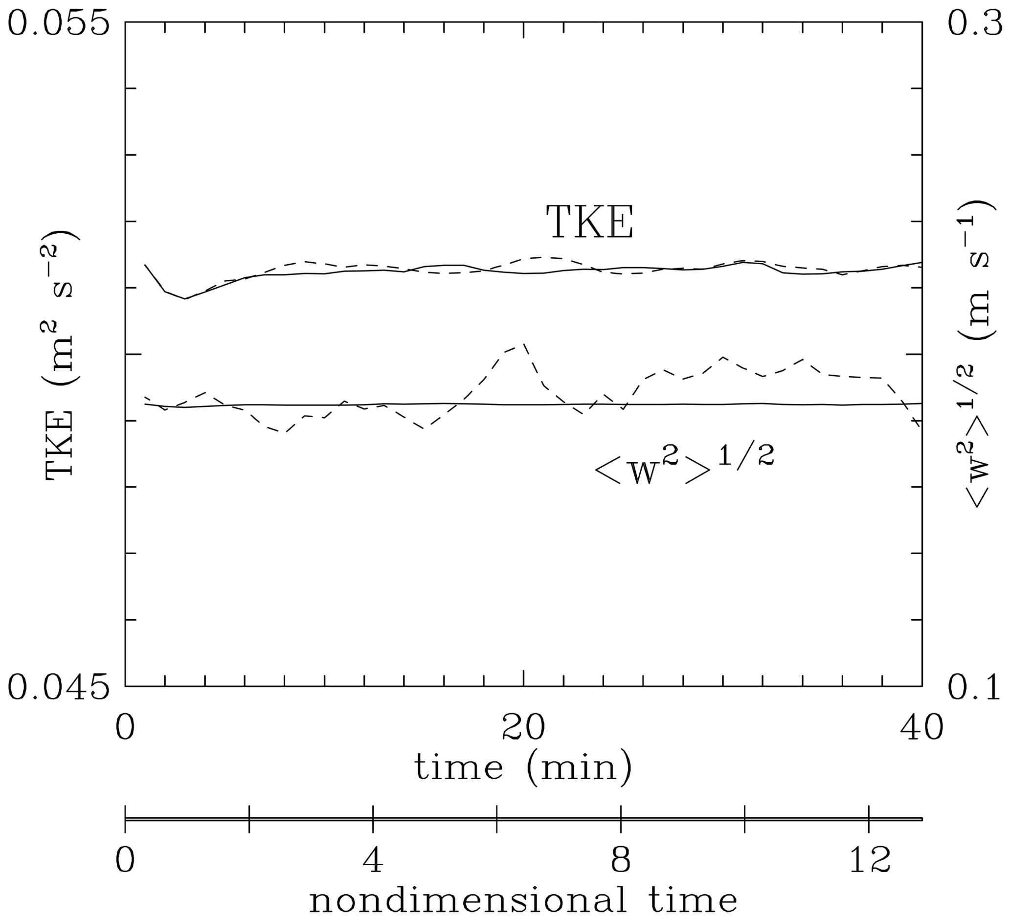
Figure 1Evolutions of the TKE and rms vertical velocity in low-TKE simulations applying either Eq. (3) (dashed lines) or Eq. (6) (solid lines), as part of the forcing. The nondimensional time is the time divided by the turbulence integral time: 187 s for the low-TKE simulations.
2.2 The setup of dynamic simulations
The triply periodic computational domain is 643 m3 with the model grid length of 1 m. This is one of the domains considered in Thomas et al. (2020) and close to the turbulent rising parcel extent of 50 m considered in Grabowski and Abade (2017). Such a domain size is also similar to the grid volume of large eddy simulations of natural clouds (e.g., Siebesma et al., 2003; Stevens et al., 2005; VanZanten et al., 2011). For the fluid flow, we consider two turbulence intensities as expressed by the prescribed TKE. The “low-TKE” simulations assume a TKE of m2 s−2. Such a TKE corresponds to the TKE dissipation rate of 10−3 m2 s−3 in 643 m3 scaled-up DNS simulations in Thomas et al. (2020) that followed DNS simulations in Lanotte et al. (2009). The low-TKE setup corresponds to the rms vertical velocity of around 0.2 m s−1 (see Fig. 1), an evolving maximum vertical velocity between 0.5 and 0.8 m s−1, and an integral timescale (see Eq. 7 in Grabowski and Abade, 2017) of 187 s or about 3 min. The model time step for the low-TKE simulations dictated by the CFL (Courant–Friedrichs–Lewy) stability criterion is Δt=0.25 s. The low-TKE dry dynamics simulations (i.e., solving only Eqs. 1 and 2) and simulations without droplets (Sect. 3) were run for 40 min (around 12 integral timescales as shown in Fig. 1). Simulations with droplets discussed in Sect. 5 were run for 20 min or about 6 integral timescales starting from minute 28 of 40 min simulations presented in the next section. The “high-TKE” simulations consider a 100 times larger TKE, i.e., 5.2 m2 s−2. High-TKE simulations feature 10 times larger rms and maximum velocities (i.e., around 2 m s−1 and 5 to 8 m s−1, respectively) together with a 10 times smaller integral timescale of about 19 s. The model time step in high-TKE simulations was proportionally reduced to 0.025 s. The high-TKE simulations were run for the same number of time steps as the low-TKE simulations, that is, for the total time of either 4 or 2 min, that is, either 12 or 6 integral timescales. Model data were saved every s for low/high-TKE simulations, and they are used in the analysis presented here.
Equation (4) allows the estimation of the TKE dissipation rate. The parameter α in the forcing term is monitored from time step to time step during the simulations. The typical value in both low and high TKE is . With the target TKE m2 s−2 and Δt=0.25 s in low-TKE simulations, the TKE dissipation diagnosed from Eq. (4) is m2 s−3. This value approximately agrees with the assumed low-TKE turbulence simulation setup. For the high TKE, the target TKE and the model time step imply m2 s−3. This is a rather extreme TKE dissipation rate for small cumulus dynamics (e.g., Siebert et al., 2006) but perhaps not unusual for deep convection as simulated, for example, by Benmoshe et al. (2012).
Figure 1, already mentioned in Sect. 2.1, documents TKE evolution together with the rms vertical velocity in the low-TKE simulation. The horizontal axis shows either the real time or the nondimensional time using the integral timescale. As the figure shows, the forcing maintains the TKE and rms vertical velocity as expected by the forcing design. Figure 2 shows the TKE spectra for low and high TKE at the minute that are used as initial conditions for moist simulations with droplets. The spectra have a classical shape characteristic of a relatively low-Reynolds-number homogeneous isotropic numerical turbulence (e.g., Fig. 2 in Rosales and Meneveau, 2005). Spectra at different times are similar to those in Fig. 2 (not shown).
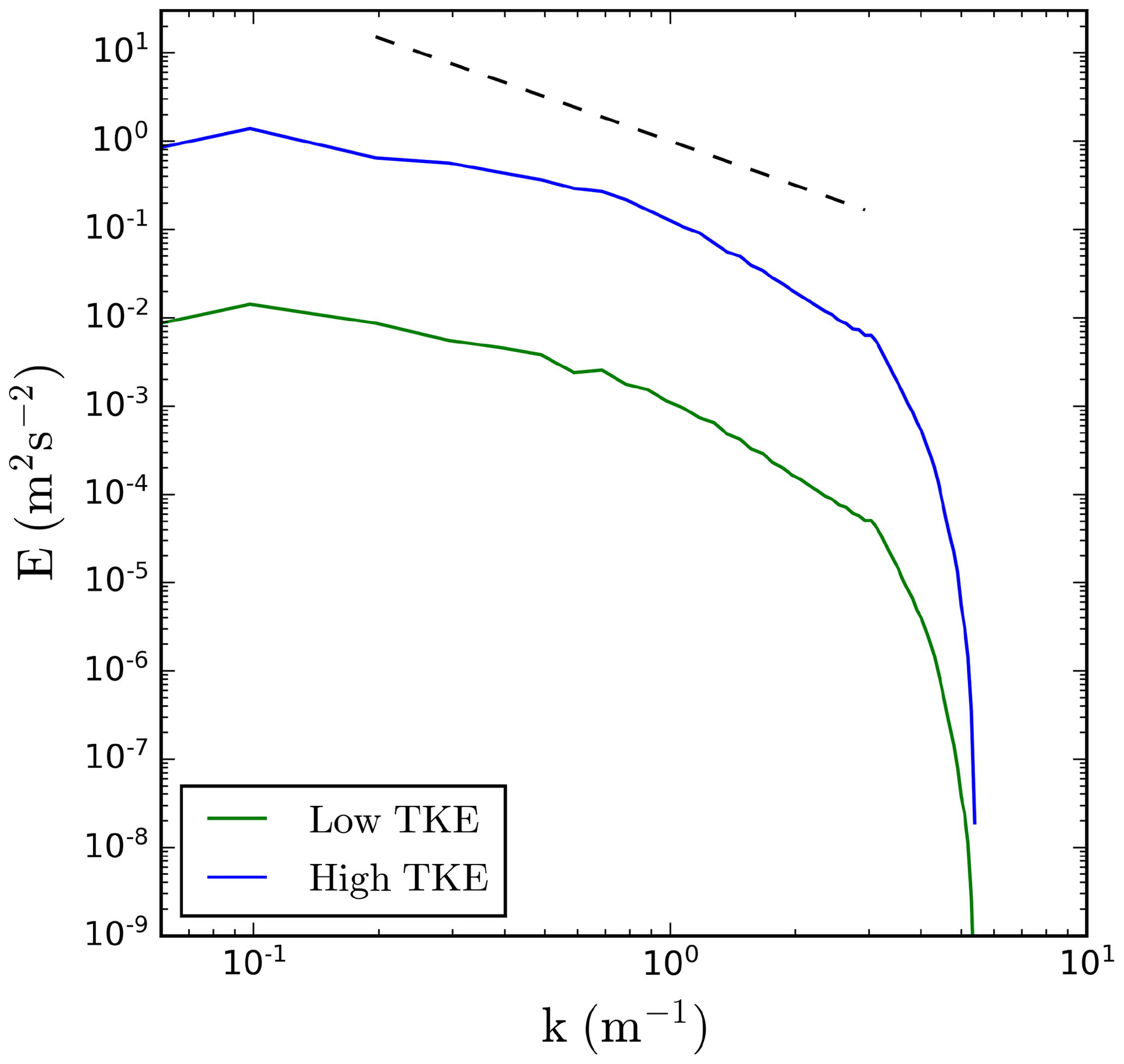
Figure 2Energy spectra for the fluid flow simulations without droplets at minute for low/high-TKE simulation without droplets. The dashed line represents the Kolmogorov slope.
The turbulence dynamics in moist simulations described in the next section is exactly as described above, that is, the impact of cloud droplets and of the latent heating on the flow is neglected. This is because the air density is assumed to be constant and the flow equations exclude the buoyancy term as typical in the homogeneous isotropic DNS simulations (see, for instance, Eq. 1 in Lanotte et al., 2009). Because the flow is exactly the same in all simulations, one can compare model results grid volume by grid volume as in the piggybacking methodology (Grabowski, 2019, and references therein). This allows a comprehensive comparison of simulation results as illustrated in Sect. 6.
In addition to the momentum, the moist ILES of homogeneous isotropic turbulence solves the temperature T and water vapor mixing ratio qv equations in the form
where J kg−1 is the latent heat of condensation, cp=1015 J kg−1 K−1 is the specific heat of air at constant pressure, g=9.81 m s−2 is the gravitational acceleration, and Cd is the condensation rate, the rate of change in the cloud water mixing ratio resulting from the diffusional growth of cloud droplets. Calculation of the condensation rate depends on the microphysics scheme as explained below and documented in Appendix B.
In the spirit of DNS studies of homogeneous isotropic turbulence, the initial temperature and water vapor mixing ratio in moist simulations are assumed to be spatially uniform. The actual values are taken as in Thomas et al. (2020); that is, T=283 K and qv at saturation assuming environmental pressure of 1000 hPa. The spatially uniform initial conditions justify the triply periodic computational domain. The last term in Eq. (6) represents the temperature change due to adiabatic air expansion resulting from the vertical motion in the stratified environment. This term drives small-scale supersaturation fluctuations in the otherwise uniform environment; see discussion in Sect. 3 in Vaillancourt et al. (2001). Such a modeling framework is a simplification of a truly stratified environment where the environmental temperature and pressure are functions of height and typically the potential temperature (an invariant for dry adiabatic vertical displacements) rather than the temperature is being applied as the model variable. In some DNS studies, the temperature and moisture equations are combined into the supersaturation equation that includes the source due to the vertical motion (as the last term in Eq. 6) and the sink due to droplet growth (Eq. (2) in Lanotte et al. (2009) or Eq. (2) in Sardina et al. (2015); see Eq. (10) below).
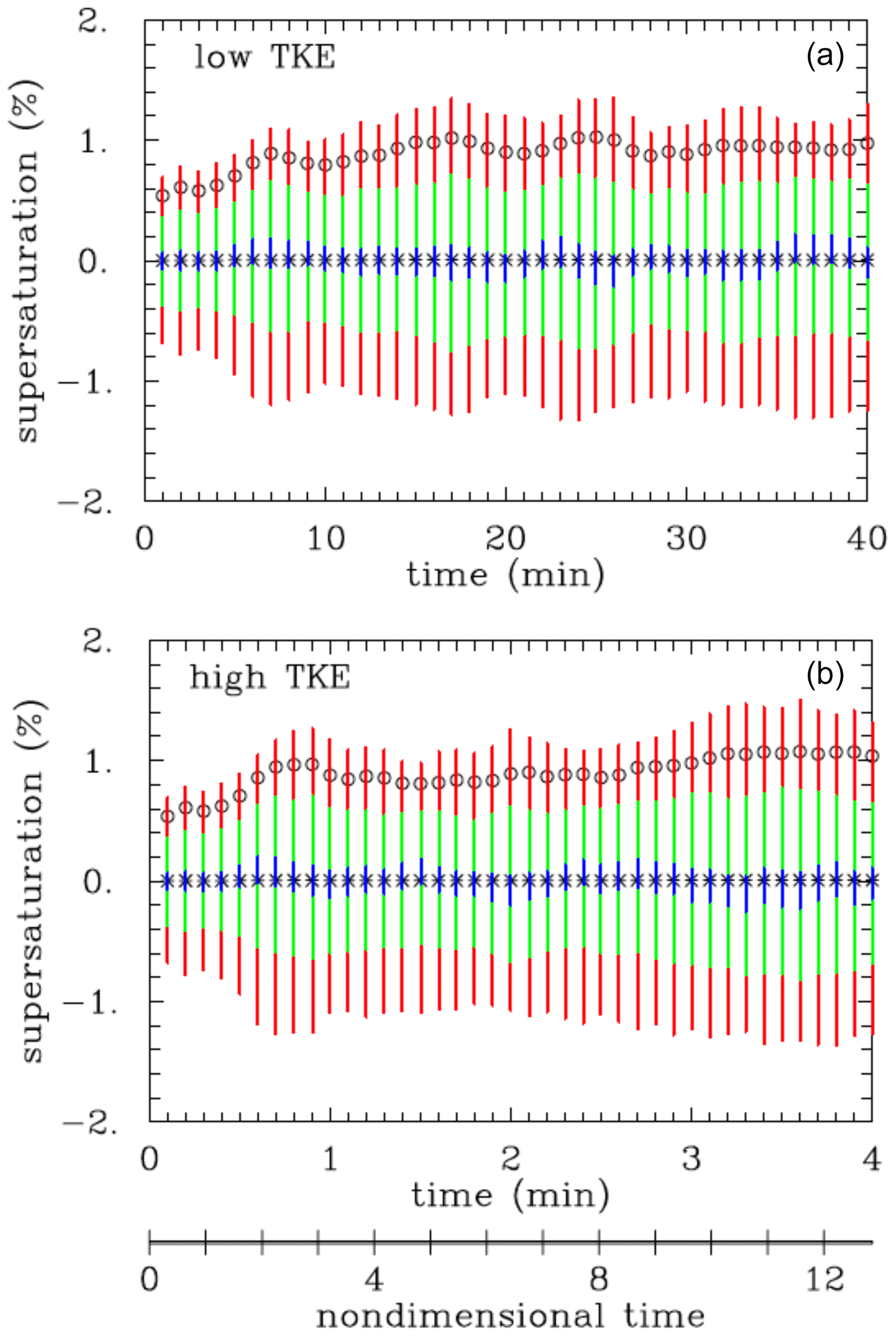
Figure 3Evolution of the supersaturation spatial distribution statistics for 40 min low-TKE (a) and high-TKE (b) moist simulations without droplets. Stars and circles show the mean and standard deviation of the spatial distribution, respectively. The extent of the color bars shows the percentiles of the distribution: red is for 10–90th percentile, green is for 25–75th percentile, and blue is for 45–55th percentile. The nondimensional time, the same for low and high TKE, is shown below (b).
The initial test of the moist ILES framework considers a 40 min long low-TKE and 4 min long high-TKE simulations without droplets (i.e., both up to about 12 integral timescales) and initiated in the same way as the dry simulation illustrated in Figs. 1 and 2. The simulations apply the fluid flow as described above and solving Eqs. (7) and (8) without the condensation term Cd. In such simulations, the largest temperature change is possible when the air parcel rises across the entire computational domain depth, that is, 64 m, with the corresponding temperature change of about 0.64 K as given by Eq. (7). Such a maximum temperature change leads to the supersaturation change from the initial zero to about 4 %. In the numerical simulation, the maximum temperature deviations from the uniform initial 283 K are typically smaller than 0.5 K. The evolutions of supersaturation statistics are shown in Fig. 3. Despite the dramatic difference in the TKE levels, the statistics are similar regardless of the TKE level, in agreement with the parcel argument. Only after including the source due to condensation do the evolutions become different depending on the droplet characteristics and the TKE level. Small differences in the evolutions in Fig. 3 come from different flow realizations between low- and high-TKE cases.
The general microphysical setup considers initially monodisperse population of cloud droplets with the radius of 13 µm present in three different concentrations: 26, 130, and 650 cm−3. The concentration 130 cm−3 was considered in Lanotte et al. (2009) and Thomas et al. (2020) and it corresponds to the mean cloud water content of about 1.2 g m−3. In addition, the 5 times smaller and 5 times larger droplet concentrations are considered to document how the two microphysics schemes represent the expected scalings. The mean cloud water content in simulations with the increased (decreased) droplet concentration is about 6.0 (0.24) g m−3. Moist simulations with droplets start at minute 28/2.8 (low/high TKE) of the moist simulation without droplets, that is, applying the flow field analyzed in Fig. 2, together with the temperature and moisture field at minute 28/2.8 in Fig. 3. The simulations are run for an additional 20 min for the low-TKE setup, saving data every 15 s. The high-TKE simulations are run for 2 min and the data are saved every 1.5 s. The data are used in the analysis of both macrophysics (e.g., the supersaturation characteristics) and microphysics (e.g., droplet spectra) simulated by the two microphysics schemes. Sardina et al. (2015) derived scalings for the case when the droplet phase relaxation time is much shorter than the turbulence integral timescale. This is the case for the selected domain size and the low TKE for all droplet concentrations. For the high TKE and low droplet concentration (i.e., 26 cm−3), the phase relaxation time (about 10 s) is the closest to the turbulence integral timescale (about 19 s), so some deviations from the theoretical scaling should be expected as shown below.
4.1 Lagrangian and Eulerian microphysics schemes
For moist simulations with droplets, Eqs. (7) and (8) are supplemented by the appropriate equations describing droplet spectral evolution. The Lagrangian scheme follows the evolution of so-called super-droplets, each representing an ensemble of real droplets, with the ensemble size referred to as the multiplicity. The bin scheme applies the Eulerian spectral density function discretized into a finite number of radius bins. Details of both approaches are presented in Appendix B.
The particle-based Lagrangian scheme considers on average 40 Lagrangian particles (super-droplets) per grid volume, each featuring the initial radius of 13 µm. The number of super-droplets per grid volume together with the assumed droplet concentration dictates the multiplicity that is assumed to be the same for all super-droplets. Although the average number of super-droplets per grid volume is small when compared to millions of real droplets within a 1 m3 grid volume, G20a and G20b document that a number as small as 10 per grid box provides physically meaningful results; see also Li et al. (2017). At the simulation onset, each super-droplet is placed at a random position within a grid volume. To be consistent with the bin microphysics, super-droplets grow in response to the mean supersaturation predicted inside a grid volume it occupies. Super-droplets are advected applying a model flow field interpolated to the droplet position as in Arabas et al. (2015). The interpolation scheme maintains the incompressibility of the flow at subgrid scales; see discussion of this aspect in Sect. 2.4 in Grabowski et al. (2018). Droplet inertia and droplet sedimentation are not considered. Condensation rate Cd at each time step is calculated by summing up the mass change in all super-droplets present within a given grid volume.
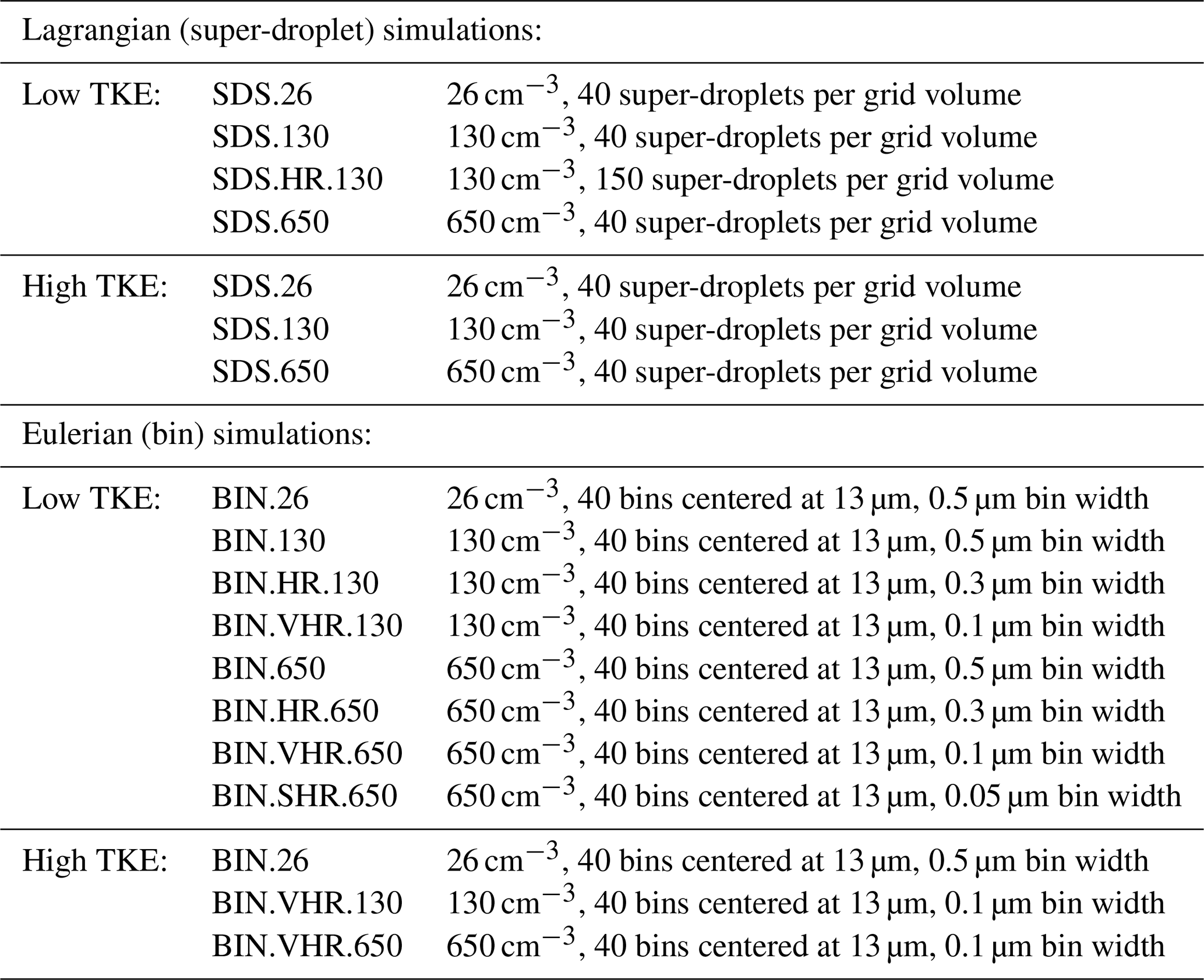
The simulations with super-droplets are referred to as SDS.26, SDS.130, and SDS.650 for a droplet concentrations of 26, 130, and 650 cm−3, respectively. The three simulations are completed for both low and high TKE. In addition, a single simulation with 150 super-droplets per grid volume and droplet concentration of 130 cm−3 was completed for the low TKE to test the impact of the super-droplet number fluctuations within a grid volume. This simulation is referred to as SDS.HR.130 (HR for high resolution in the radius space).
The Eulerian bin microphysics considers the spectral density function represented by 40 equally spaced bins with the bin size modified in different simulations as described below. The reason for modifications of the bin resolution is to match the results from the Lagrangian microphysics as shown in the results section. In each bin setup, there is a bin centered at 13 µm that is filled with droplets at the simulation onset. The monodisperse initial droplet size distribution is impossible to be accurately represented using the spectral density function because the monodisperse distribution corresponds to the delta function. However, even with a finite width of the initial distribution, the broadening of the distribution as time progresses (Sardina et al., 2015; Li et al., 2019; Thomas et al., 2020) can be appropriately represented provided that the bin width is appropriately small (see Sect. 5.3). In the bin microphysics, each bin is independently advected in the physical space using the same advection scheme that is applied to the momentum, temperature, and water vapor mixing ratio. Neither droplet sedimentation nor droplet inertia are regarded as in the Lagrangian scheme. All bins are combined at each grid volume to calculate the evolution of the droplet spectrum due to the local sub- or supersaturation applying a custom-designed 1D advection scheme. The scheme combines the analytic Lagrangian solution of the condensational growth with remapping of the spectral distribution onto the original radius grid using piecewise linear functions (see Sect. 3.2 in Grabowski et al., 2011). As for the Lagrangian scheme, condensation rate Cd at each time step is calculated from the change in the spectral density function due to the droplet growth in each grid volume; see Appendix B.
For the low TKE, eight-bin simulations with the spectral density function represented by 40 bins and different bin resolutions are considered. The selection of a specific bin resolution is motivated by the results discussed in the next section. The standard bin setup is similar to G20b with a uniform 0.5 µm bin width and 0 to 20 µm bin range. These simulations are BIN.26, BIN.130, and BIN.650 for the three droplet concentrations. The high-resolution (HR) simulations have 0.3 µm bin width and a bin layout centered at 13 µm (i.e., from 7 to 19 µm). These simulations are run for 130 and 650 cm−3 concentrations and are referred to as BIN.HR.130 and BIN.HR.650, respectively. Very high-resolution (VHR) simulations have 0.1 µm bin width, again centered at 13 µm (bin range between 11 and 15 µm) and with 130 and 650 cm−3 concentration (BIN.VHR.130 and BIN.VHR.650). Finally, an even higher bin resolution, with 0.05 µm bin width and a grid centered at 13 µm (i.e., bin range between 12 and 14 µm), is added for the 650 cm−3 concentration (BIN.SHR.650; SHR for super-high resolution). For the high TKE, only three simulations were completed: BIN.26, BIN.VHR.130, and BIN.VHR.650. Table 1 provides a list of all simulations in both Lagrangian and Eulerian simulations. Results of additional simulations with a smooth initial droplet spectrum are presented in Appendix A.
Droplet growth in both schemes is calculated applying a simplified growth formula as in G20a and G20b:
with m2 s−1 and r0=1.86 µm. The latter is applied to mimic the impact of kinetic effects (Mordy, 1959; see Eq. 11 in Clark, 1973, or Eq. 2.22 in Kogan, 1991). Because of a large mean droplet size of 13 µm, the solution and curvature effects are neglected. The two schemes apply the droplet growth Eq. (9) in different ways: as transport (advection) velocity in the Eulerian bin scheme and to calculate individual super-droplet growth in the Lagrangian scheme; see Appendix B.
5.1 Lagrangian microphysics
Figure 4 shows evolutions of the supersaturation standard deviation in low- and high-TKE Lagrangian simulations. The supersaturation standard deviation is approximately constant except for the adjustment from initial values in simulations without droplets (see Fig. 3). Standard deviations for the SD.130 and SD.HR.130 simulations are practically the same. Table 2 shows the standard deviation averaged over the second half of the simulations. When the phase relaxation time is much smaller than the turbulence integral timescale, the supersaturation standard deviation is proportional to the product of the rms vertical velocity and the phase relaxation time; ; see Sardina et al. (2015). The phase relaxation time is inversely proportional to the product of the mean droplet radius and droplet concentration. With the same mean droplet radius, changes in the concentration explain shifts of a factor of about 5 between SDS.650, SDS.130, and SDS.26 for the low-TKE case as shown in Fig. 4a and in Table 2. However, for the high TKE, the scaling breaks down because the phase relaxation time is no longer much smaller than the turbulence integral timescale. For a given droplet concentration, shift from low to high TKE should result in a 10-fold increase in σS because of the increase. This is approximately valid for 650 cm−3 droplet concentration but reduces to a factor of only about 5 for 26 cm−3 concentration.
The supersaturation standard deviation shown in Fig. 4 can be compared to the standard deviation resulting from the quasi-equilibrium supersaturation fluctuations. The evolution of the supersaturation (where qvs is the saturated water vapor mixing ratio) can be derived by combining Eqs. (7), (8) and (9) as
where τrelax is the phase relaxation time that depends on the mean droplet radius and concentration:
where ρw=103 kg m−3 is the water density, Rv=461 J kg−1 K−1 is the water vapor gas constant, and in Eq. (11) depicts averaging over all droplets within a given grid volume. The quasi-equilibrium supersaturation is obtained by setting the left-hand side of Eq. (10) to zero, which leads to Seq=a1wτrelax. For the mean temperature and humidity of the simulations and specific numerical values of the relevant constants, m−4 and the phase relaxation time for the 13 µm droplets and their concentration of 130 cm−3 is τrelax=1.98 s. The phase relaxation time is 5 times smaller/larger for the droplet concentration of cm−3. Since the quasi-equilibrium supersaturation is proportional to the vertical velocity, its standard deviation is proportional to the rms vertical velocity. For the low TKE, the quasi-equilibrium supersaturation standard deviation is 0.120 %, 2.39 %, and 4.79 % for 26, 130 and 650 cm−3 droplet concentrations. These are in a relatively good agreement with the simulated standard deviation shown in Table 2. The values for the high TKE should be 10 times smaller and they are approximately equal to the simulated values for 130 and 650 cm−3. The agreement between the simulated supersaturation fluctuations and the fluctuations predicted by the quasi-equilibrium supersaturation for the 643 m3 domain and low TKE agrees with results presented in Thomas et al. (2020; see Fig. 10 therein and its discussion).
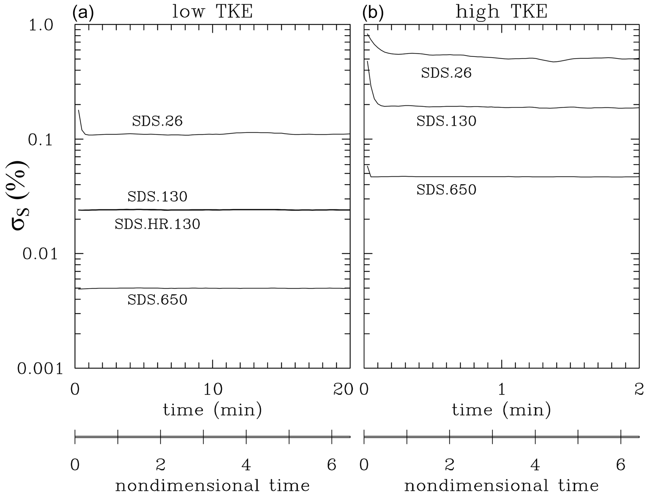
Figure 4Evolution of the supersaturation standard deviation in (a) four low-TKE simulations and (b) three high-TKE simulations with super-droplets. The two simulations with droplet concentration of 130 cm−3 in panel (a), SDS.130 and SDS.HR.130, show differences within the thickness of the line.
Figure 5 shows the comparison between the local supersaturation simulated by the model and the quasi-equilibrium supersaturation calculated applying the local vertical velocity and the mean phase relaxation time for the low- and high-TKE simulations and 26 versus 650 cm−3 droplet concentrations. The mean phase relaxation time is about 10 s for 26 cm−3 and about 0.4 s for 650 cm−3 droplet concentrations. Whether the quasi-equilibrium supersaturation is a good approximation of the local supersaturation depends on the relative magnitude of the phase relaxation timescale and the eddy turnover time associated with the largest eddies. This is because the largest eddies feature the largest vertical velocities and provide the strongest forcing to drive the supersaturation away from its quasi-equilibrium value. For the low TKE, the eddy turnover time for the largest eddies is about 1 min (i.e., velocities up to 0.8 m s−1 and the domain size of 64 m), much larger than the phase relaxation time for both concentrations shown in Fig. 5. This is why all points scatter around the 1:1 line in Fig. 5a and c. However, the eddy turnover time is only around 8 s for the high-TKE case. This is still much larger than the phase relaxation time for the 650 cm−3 droplet concentration (Fig. 5d), but close to the phase relaxation time for the 26 cm−3 concentration. This is why data points are scattered away from the 1:1 line in Fig. 5b, with the quasi-equilibrium values typically larger (in the absolute sense) than the model-predicted supersaturation.
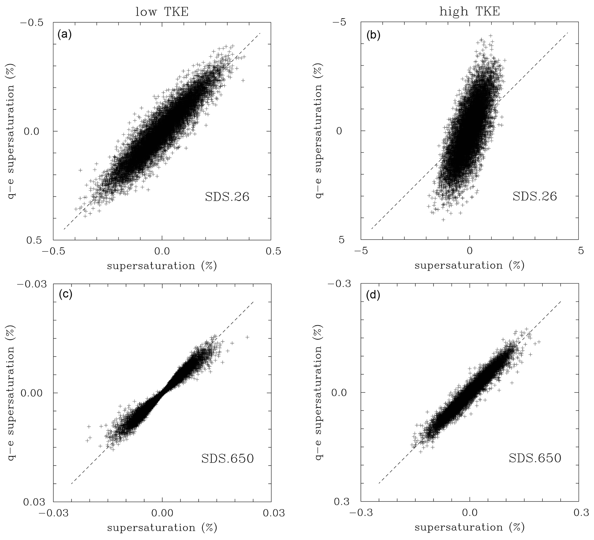
Figure 5Comparison between supersaturation simulated by the model (horizontal axes) and the quasi-equilibrium supersaturation calculated with the local vertical velocity and the mean phase relaxation time (vertical axes) for (a, c) low TKE and (b, d) high-TKE simulations. Simulations SDS.650/SDS.26 are in the lower/upper panels. Data from the last time level of all simulations with only 5 % of data points are shown. Note different supersaturation ranges in all panels.
Figure 6 shows evolutions of the radius-squared standard deviation. Sardina et al. (2015) show that the standard deviation of the radius-squared distribution should increase in time as a square root of time as long as the phase relaxation time is much smaller than the turbulence integral time. The rate of increase is proportional to the supersaturation standard deviation (see Eq. 13 in Sardina et al., 2015). The scaling has been shown in other numerical simulations, such as in Li et al. (2019) and Thomas et al. (2020). Figure 6 shows that the Lagrangian microphysics reproduces the scaling and that the differences between various simulations for the low TKE can be explained by the differences in the supersaturation standard deviation shown in Fig. 4 (note that on the log–log plot the rate of increase change corresponds to a vertical shift as shown in Fig. 6). For the high TKE, small deviations for the expected scaling can be explained by the phase relaxation time being no longer much smaller than the turbulence integral time. This is especially evident for the high-TKE SDS.26 case in Fig. 6b. Figures. 4a and 6a show that increasing the number of super-droplets from 40 to 150 per grid volume has virtually no impact on the results. Overall, the Lagrangian microphysics seem to represent expected scalings (or departures from them) without much difficulty.
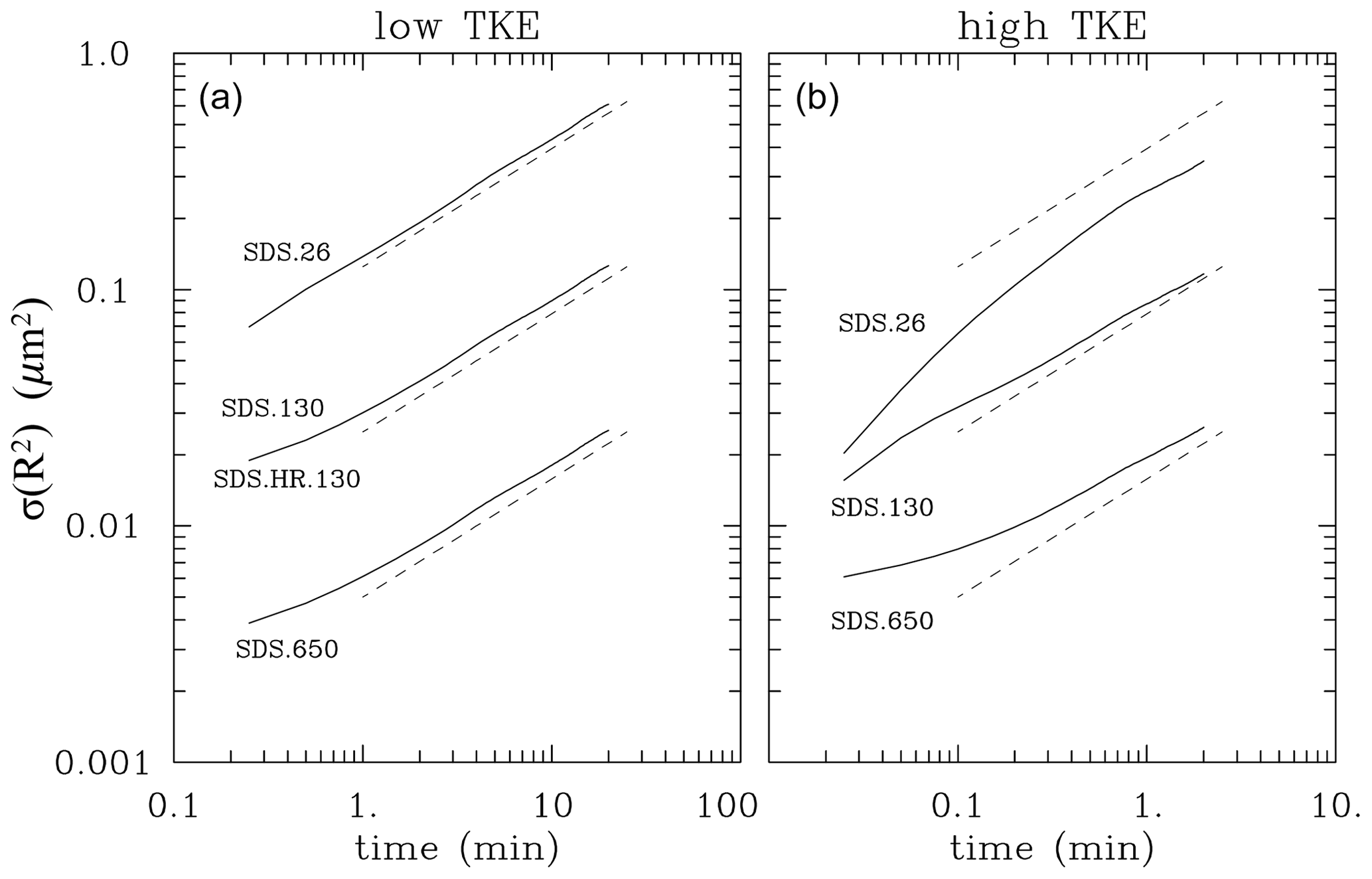
Figure 6Evolution of the radius-squared standard deviation for super-droplet simulations: (a) four low-TKE simulations and (b) three high-TKE simulations with super-droplets. SDS.130 and SDS.HR.130 in (a) differ by the thickness of the line. Dashed lines show the expected scaling and are spaced by the expected factor of 5. Their position is the same in (a) and (b).
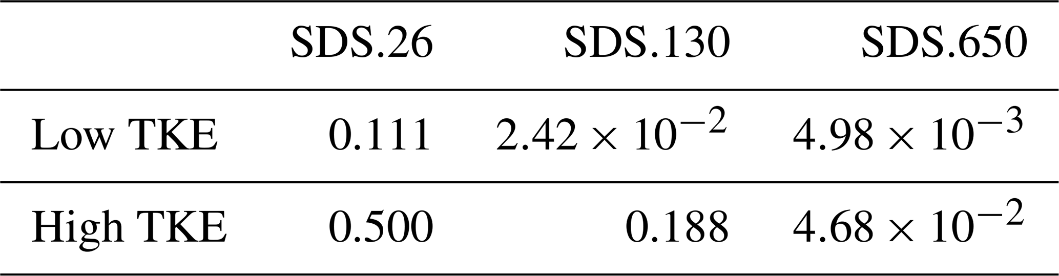
Table 2Supersaturation standard deviation ( %) averaged over the last three integral timescales for Lagrangian microphysics simulations.
5.2 Eulerian bin microphysics
Figures 7 and 8 show the same results as Figs. 4 and 6 for the bin microphysics. For the supersaturation fluctuations (Fig. 7), bin simulations match Lagrangian microphysics results, and the impact of bin resolution is small, at least for the low-TKE simulations which feature various bin resolutions. However, as shown in Fig. 8, the expected scaling requires appropriately high bin resolution, and the resolution requirement changes depending on the droplet concentration. The standard bin resolution is sufficient for the BIN.26 simulation. However, 130 cm−3 simulations require a VHR setup (bin width of 0.1 µm) to match the expected scaling. Even the SHR setup (bin width of 0.05 µm) is insufficient for the 650 cm−3 droplet concentration. There are some similarities between Lagrangian and Eulerian results for the high-TKE simulations, that is, when the scalings derived by Sardina et al. (2015) may not apply. Figure 8a also shows the decrease in the initial radius-squared standard deviation with the increase in the bin resolution. This comes from the ill-posedness of the initially monodisperse droplet size distribution for the bin microphysics. The comparison between the local supersaturation predicted by the model and the quasi-equilibrium supersaturation calculated using the local vertical velocity (i.e., Fig. 5) for the bin microphysics is similar to that shown for the Lagrangian scheme and is not shown.
In summary, Eulerian bin microphysics are capable of appropriately representing turbulent temperature and moisture fluctuations but fail to simulate their impact on droplet spectra unless an appropriately high bin resolution is used. This is further supported by the comparison of droplet spectra discussed in the next section.
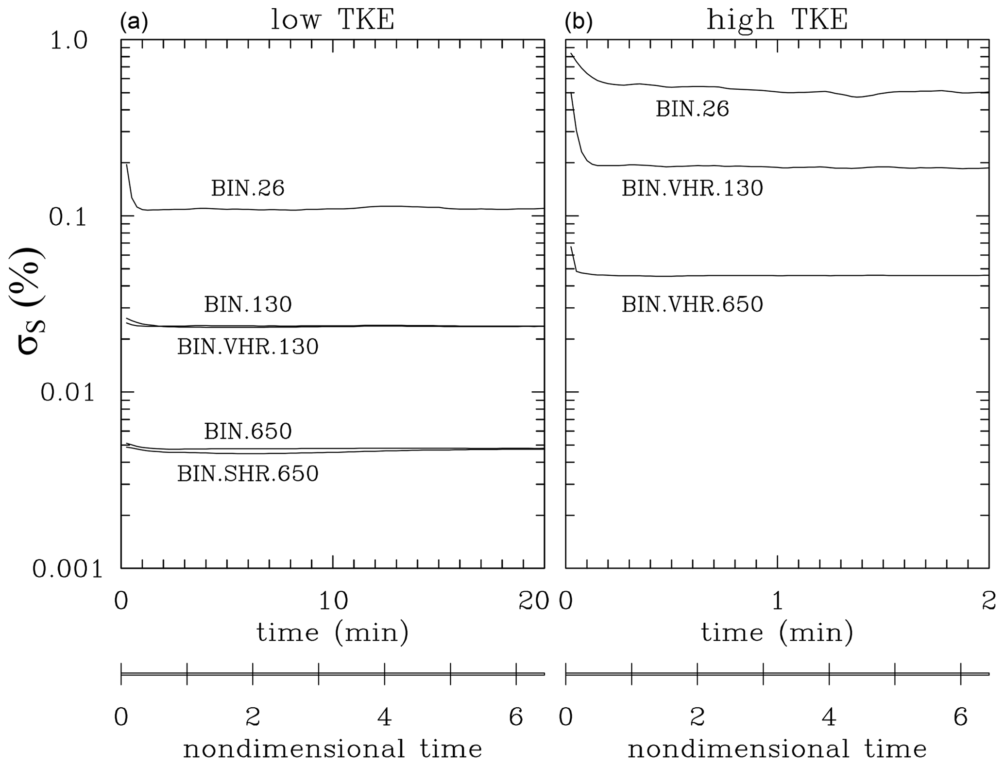
Figure 7As Fig. 4 but for the supersaturation standard deviation in eight simulations with bin microphysics.
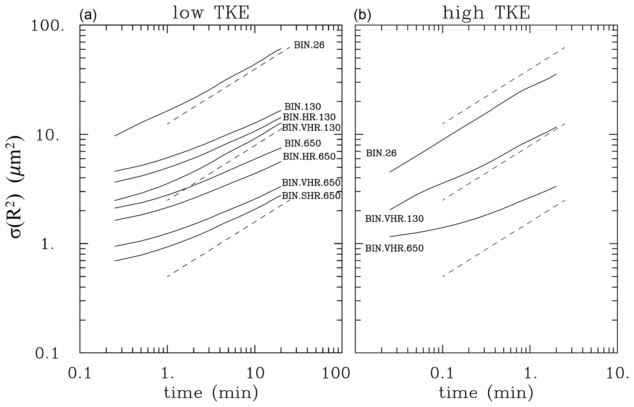
Figure 8Evolution of the radius-squared standard deviation for bin simulations. Dashed lines show the expected scaling. Their positions are exactly as in Fig. 6 for the Lagrangian microphysics.
5.3 Comparison of radius-squared distributions between Eulerian and Lagrangian simulations.
This section compares radius-squared (R2) distributions at the end of the simulations, that is, after six turnover times, for both the low- and high-TKE simulations. As shown in Lanotte et al. (2009) and Sardina et al. (2015), an initial monodisperse distribution should evolve into a Gaussian R2 spectrum because of the parabolic cloud droplet growth equation. Although the parabolic growth is only approximately valid because of the specific droplet growth equation (see Eq. 9), the Gaussian distribution is a good fit for simulation results discussed here as shown below.
Figure 9 shows the spectra for selected super-droplet simulations. The radius-squared spectra are created by selecting R2 bin size and binning super-droplet radii for a given simulation into the assumed bin grid. The bin size for the SDS.650/SDS.26 simulations (lower/upper panels in Fig. 9) is µm2. There are two panels for each simulation: one with the linear vertical scale and the spectrum shown as a histogram and the second one with the logarithmic vertical scale and using star symbols to show the spectrum. In addition, the logarithmic plots show the Gaussian distributions obtained with the mean and standard deviation calculated from the spectra.
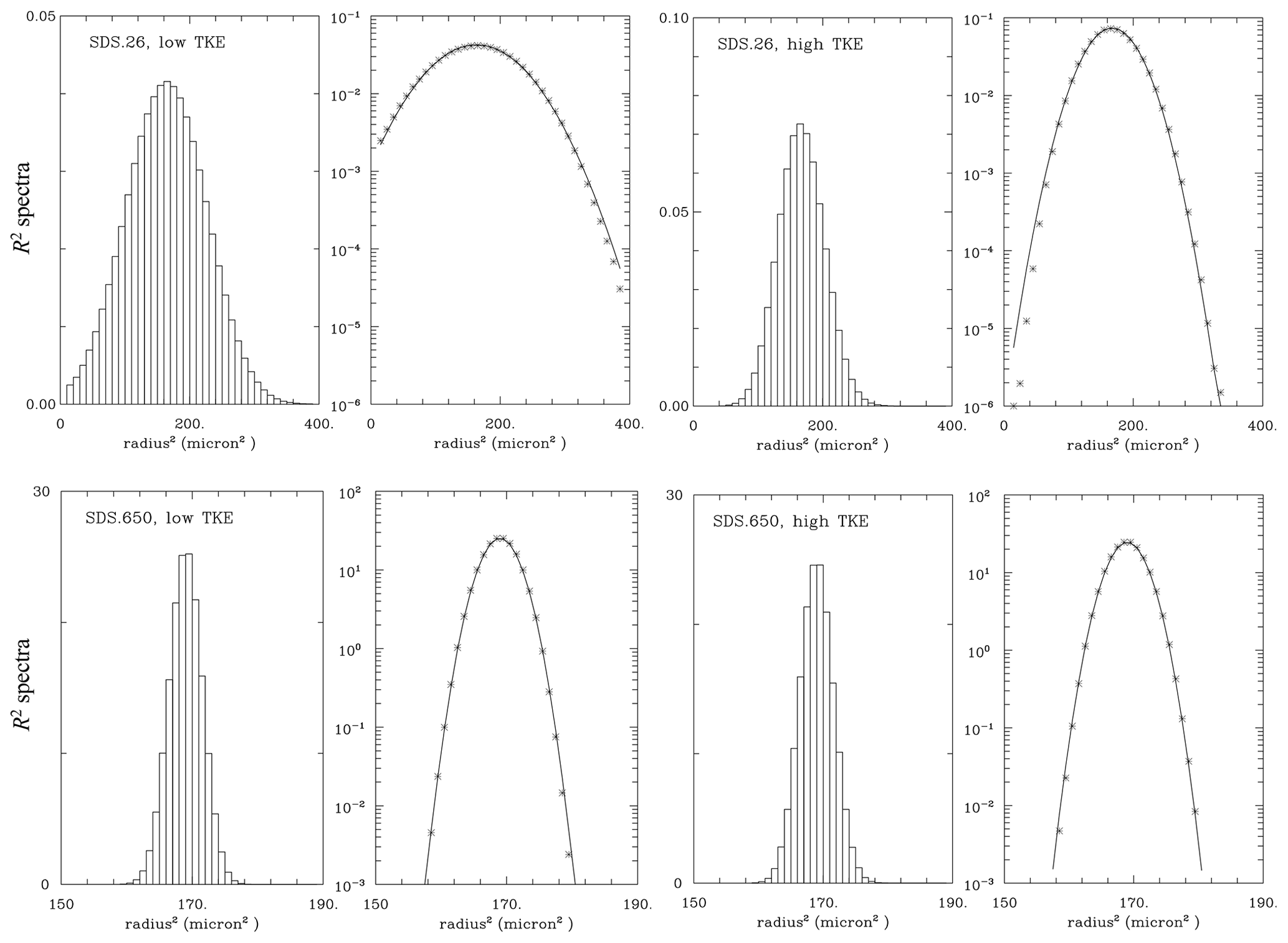
Figure 9Results from simulations (upper panels) SDS.26 and (lower panels) SDS.650 super-droplet simulations. There are two panels for each simulation, the left one applying the linear vertical scale and the right one applying the logarithmic scale. The line in the logarithmic scale panels shows the Gaussian distribution with the mean and standard deviation calculated from the spectrum. The left/right pair in each row is for the low/high-TKE simulation.
For the SDS.650 simulations (lower panels in Fig. 9), the spectra at the end of low- and high-TKE simulations are practically the same. This agrees with the theoretical scaling and simulation results shown in Figs. 4 and 6. In contrast, results for SDS.26 differ drastically between the low and high TKE. The spectrum for the low TKE is wide, with some small droplets already evaporated because the spectrum is truncated at the low-radius end. Nevertheless, the Gaussian shape is still a good fit for the simulated spectrum. The high-TKE SDS.26 spectrum is significantly narrower with small deviations from the Gaussian fit.

Figure 10As Fig. 9, but for the bin (upper panels) BIN.26 and (lower panels) BIN.VHR.650 simulations.
Figure 10 shows the spectra for bin simulations similar to those in Fig. 9. Since bin simulations predict the spectra directly, the radius spectra are converted to R2 spectra and then plotted at their native resolution in the R2 space. This explains the change in the resolution along the horizontal axes evident in the upper panels. Overall, there are some similarities between Figs. 9 and 10. For instance, upper panels show spectra for the 26 cm−3 simulations with 0.5 µm bin width that are similar to those in super-droplet simulations. Spectra for 650 cm−3 simulations with 0.1 µm bin width (i.e., from the VHR set) are also similar between low- and high-TKE simulations, but their spectral widths are larger than in corresponding panels of Fig. 9. The impact of the bin resolution is further documented in Fig. 11, which shows results from the 650 cm−3 low-TKE HR and SHR simulations, that is, with the bin width of 0.3 and 0.05 µm, respectively. Only the SHR simulation (i.e., the right panel in Fig. 11) resembles the spectra from the Lagrangian simulations shown in the lower panels of Fig. 9.
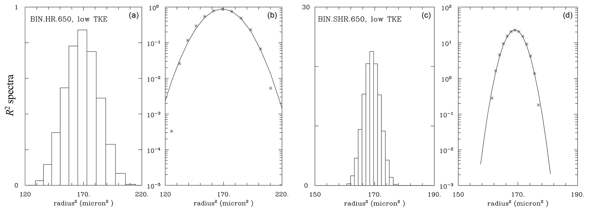
Figure 11As Figs. 9 and 10, but for the bin BIN.HR.650 and BIN.SHR.650 simulations. Note different horizontal range in (a, b) and (c, d).
In summary, only extreme resolutions of the bin scheme (e.g., as in SHR, 0.05 µm bin width) allow good agreements between Lagrangian and Eulerian results for the concentration range considered here. Moreover, the ill-posed initial condition for the Eulerian scheme (i.e., the monodisperse initial droplet size distribution) seems irrelevant because the spectrum becomes well-resolved after some time during the simulation. With a sufficiently high bin resolution (e.g., 0.5 µm in the 26 cm−3 simulations or 0.05 µm for the 650 cm−3 simulations), the Eulerian and Lagrangian spectra compare well at the end of the simulations. This shows the benefit of the Lagrangian scheme as one does not have to worry about the bin size to obtain numerically converged solutions.
The analysis presented in previous sections concerns domain-averaged characteristics. Because all simulations with either low or high TKE feature exactly the same evolving flow field, simulated thermodynamic variables (i.e., the temperature, water vapor, and cloud droplet characteristics) can be compared grid volume by grid volume and thus provide a comprehensive comparison of simulated local conditions. Such a comparison is in the spirit of the piggybacking methodology applied in G20b.
Figure 12 compares the temperature, water vapor, and cloud water mixing ratios (the latter derived from the predicted droplet spectra within each grid volume) between SDS.130 and BIN.130 low-TKE simulations at the time of 20 min. For the temperature and moisture, plots at earlier times are similar to Fig. 12a and b except for smaller ranges between minima and maxima. Cloud water plots at earlier times are also similar to those shown in Fig. 12 except for the initial couple minutes. The temperature and water vapor values are extremely close between the two simulations: the root mean square difference between temperatures is K. For the water vapor mixing ratios, the root mean square difference is g kg−1. However, the cloud water mixing ratio can differ significantly between the bin and the super-droplet simulations. This is because of statistical fluctuations in the number of super-droplets per grid volume. With on average 40 super-droplets per grid volume, the standard deviation of the droplet number is around 6 or about 15 % of the mean. Assuming that one can find grid volumes with 3 times the standard deviation, the range of the cloud water mixing ratio can be as high as close to 50 %. This can explain the spread seen in Fig. 12c. With 150 super-droplets per grid volume in SDS.HR.130, there is some improvement as the standard deviation is reduced to about 8 % of the mean, but the statistical fluctuations remain significant. In fact, panel c does not change significantly if SDS.130 is replaced by SDS.HR.130 (not shown). Figure 12d shows the outcome of a simple rescaling of the cloud water mixing ratio qc predicted by the Lagrangian scheme based on the number of super-droplets N being present in a given grid volume compared to the expected mean value of 40, with the rescaled cloud water mixing ratio given by (i.e., increased when N<40 and reduced when N>40). We stress that the rescaling is done on the analyzed cloud water and not during the model run. (That said, the application of such a rescaling might be a valuable approach to reduce the spread during model run as well; this aspect is left for a future investigation.) Apparently, the rescaling improves the comparison significantly and documents that the scatter present in Fig. 12c comes predominantly from the statistical fluctuations in the Lagrangian scheme. An important point is that the cloud water fluctuations are short-lived. This is because the temperature and water vapor would feature larger scatter if the fluctuations in the grid-volume super-droplet number were long-lived. These statistical fluctuations come only from super-droplet advection by the resolved flow as the inertial effects and droplet sedimentation are not considered.
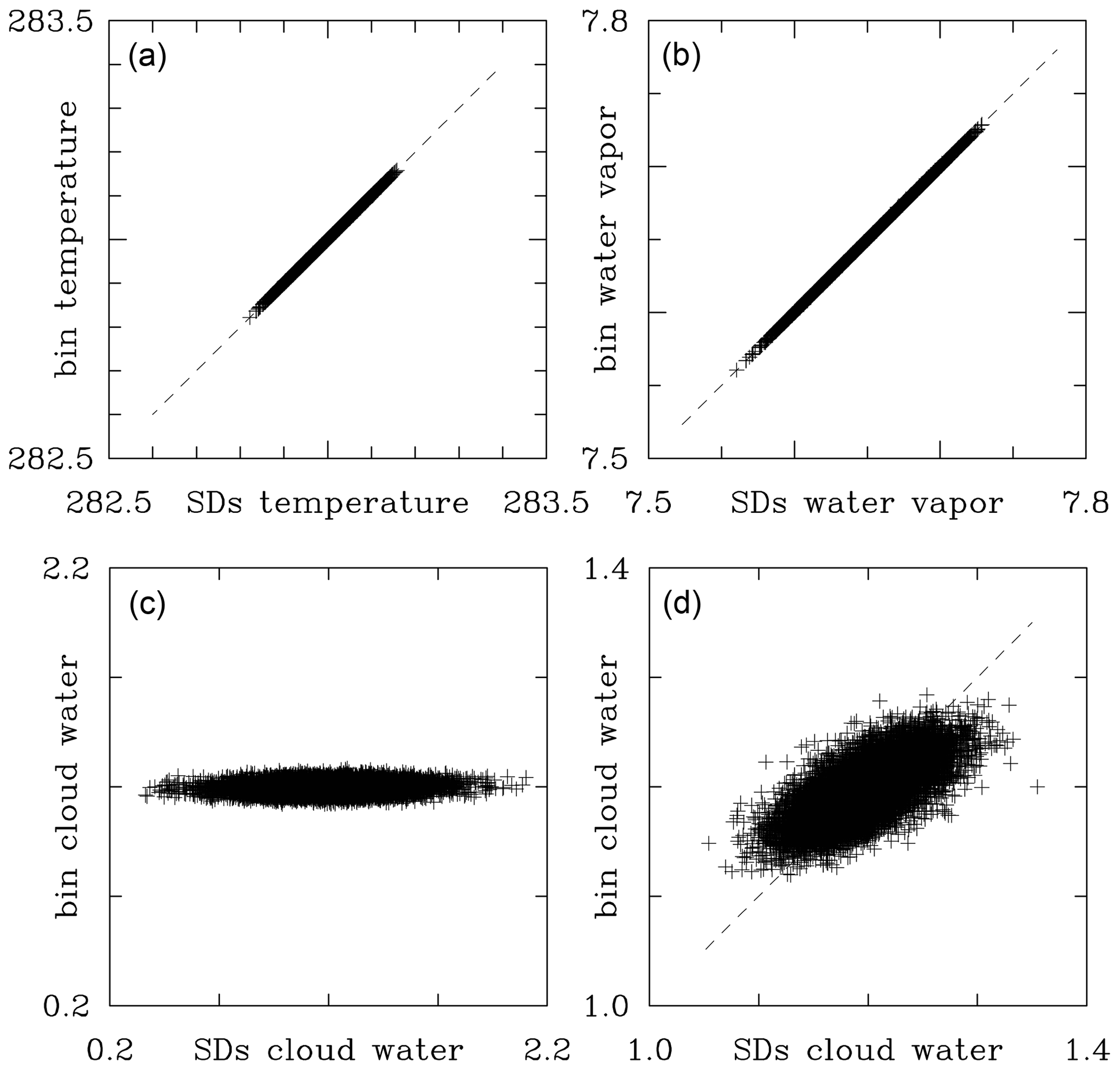
Figure 12Grid-volume by grid-volume comparison for the low-TKE SDS.130 and BIN.130 simulations between (a) temperature (in K), (b) water vapor mixing ratio (in g kg−1), and (c) cloud water mixing ratio (in g kg−1) at minute 20. Panel (d) shows cloud water mixing ratio comparison after the SDS.130 results are adjusted as explained in the text. Note the change in horizontal and vertical scales between (c) and (d). Only 5 % of data points is used.
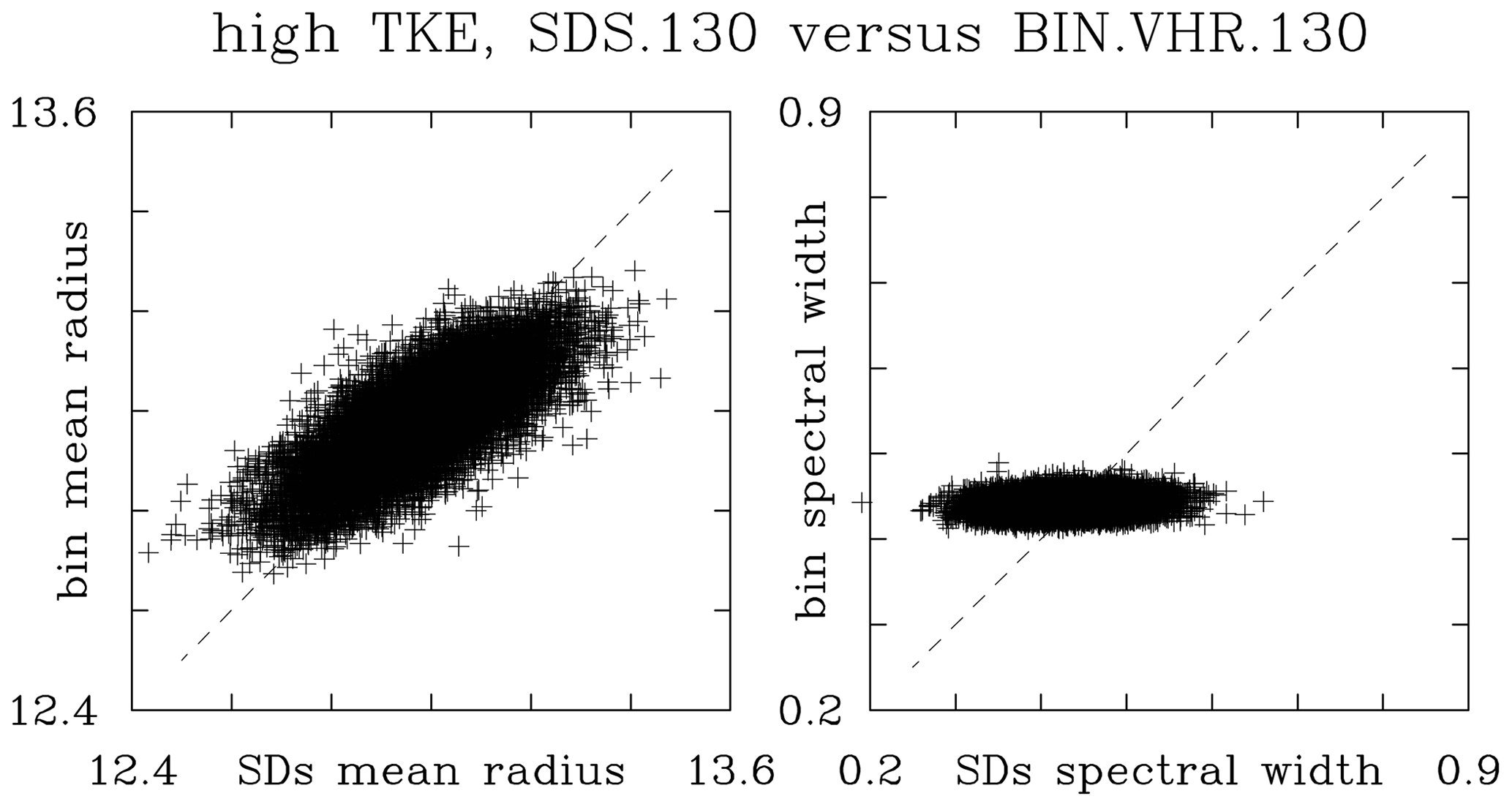
Figure 13, in the format of Fig. 12, compares the grid-volume mean radii and spectral width in two sets of low-TKE simulations: the standard resolution (SDS.130 and BIN.130) and the increased resolution (SDS.HR.130 and BIN.VHR.130). For the increased bin resolution, the selected bin microphysics are those that show the correct scaling in Fig. 8. The mean radius comparison features some scatter that is reduced when increased-resolution simulations are compared. However, the scatter is asymmetric with respect to the 1:1 line and similar to the cloud water scatter in the Fig. 12d. The asymmetry shows that the bin microphysics tend to simulate larger droplets than the Lagrangian microphysics for droplets smaller than the mean, and the reverse is true for droplets larger than the mean. The spectral width panels show that the bin simulations feature smaller spread of the spectral width across the computational domain than the Lagrangian scheme. This seems independent of the bin resolution. In other words, spectral width simulated by the bin scheme varies less across the computational domain. In contrast, super-droplet simulations feature larger spread of the spectral width across the domain, and the spread decreases with the increase in the mean super-droplet number per grid volume. For the SDS.130 versus BIN.130 cloud of spectral width points (i.e., Fig. 12b), the center of mass is above the 1:1 line. This implies that the mean spectral width for the BIN.130 simulation is overpredicted, in agreement with the results shown in Fig. 8. Results for similar comparisons of other simulations (for instance, SDS.26 versus BIN.26 or SDS.650 and BIN.SHR.650) are similar except for different ranges of the mean radius and spectral width (not shown). As shown in Fig. 14, the high-TKE simulations also show similar patterns, with changes consistent with the differences in Figs. 6b and 8b.
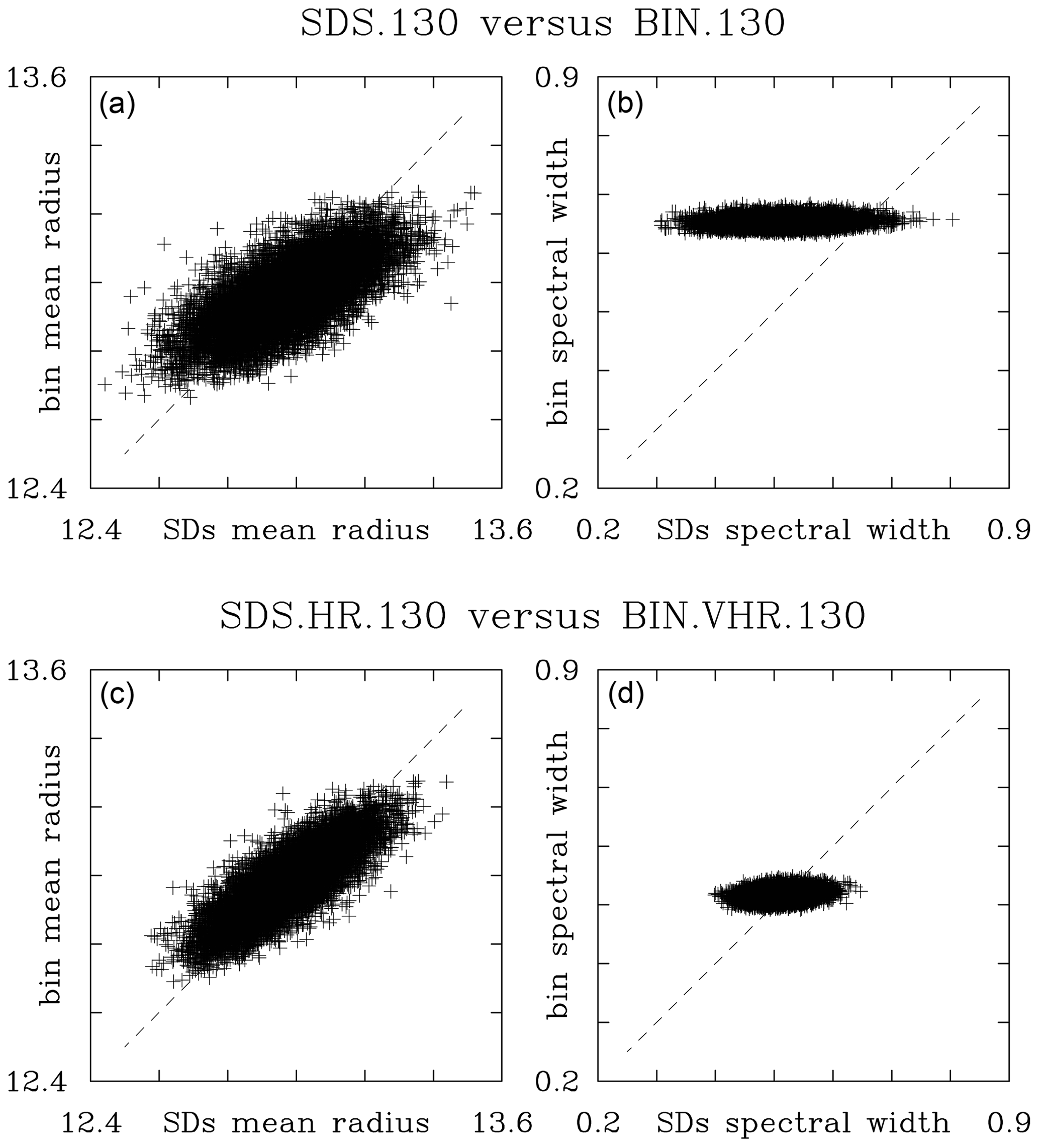
Figure 13Grid-volume by grid-volume comparison at the end of low-TKE simulations (20 min) between (a, c) (the grid-volume mean radius, in µm) and (b, d) are for comparison between SDS.HR.130 and BIN.VHR.130 (SDS.130 and BIN.130). Only 5 % of data points is used.
In summary, the grid-volume by grid-volume comparison between Eulerian and Lagrangian results shows that the simulated spatial variability is smaller in the bin microphysics when compared to the super-droplets. Arguably, this comes from a combination of the numerical diffusion in the bin microphysics (i.e., smoothing bin results similar to other Eulerian fields) and small-scale fluctuations of the Lagrangian microphysics due to a relatively small mean number of super-droplets per grid volume.
This paper presents a modeling study addressing the impact of homogeneous isotropic turbulence on the broadening of an initially monodisperse distribution of cloud droplets in response to local fluctuations of the supersaturation field. This problem has been considered previously in modeling studies of Lanotte et al. (2009) applying DNS, Thomas et al. (2020) using the scaled-up DNS, and Sardina et al. (2015) employing theoretical analysis combined with DNS and stochastic model simulations. Sardina et al. (2015) derived scaling relationships that we use in validating model results and comparing results for different droplet concentrations and contrasting turbulence intensities.
Because we apply a finite-difference fluid flow model, we had to develop a turbulence forcing scheme that led to the quasi-steady homogeneous isotropic turbulence similar to that simulated by a spectral model. The forcing scheme applied here is in the spirit of the linear forcing of Rosales and Meneveau (2005) and Onishi et al. (2011). The idea is to ensure that the mean turbulence kinetic energy (TKE) remains constant in time and that the partitioning between the three TKE components does not change. The latter is important for the simulations of the turbulence impact on the droplet spectra because the driving mechanism in the homogeneous environment comes from the vertical velocity fluctuations affecting the local supersaturation. The simulations are in the spirit of the implicit large eddy simulation (ILES), that is, without modeling the small-scale TKE and scalar variance dissipation (Margolin and Rider, 2002; Andrejczuk et al., 2004; Margolin et al., 2006; Grinstein et al., 2007). ILES applying a finite-difference model relies on the model numerics to provide the required dissipation, in contrast to the scaled-up spectral model DNS in Thomas et al. (2020), where appropriately scaled-up molecular dissipation coefficients have to be used to ensure stable simulations. The TKE dissipation rate diagnosed from the forcing algorithm (see Eq. 6) is approximately correct for the considered turbulence intensities.
There are two drastically different simulation techniques that can be applied to investigate the impact of cloud turbulence on the droplet spectra: the Eulerian bin microphysics and the Lagrangian particle-based approach, the latter often referred to as the super-droplet method (see review in the Introduction). We apply the ILES homogeneous isotropic turbulence setup to compare the two techniques following Li et al. (2017) and Grabowski (2020a, b) for the diffusional growth of cloud droplets only. The computational domain is 643 m3, one of the domain sizes considered in Thomas et al. (2020) and similar to grid volumes of a typical large eddy simulation of natural clouds. Two TKE intensities are considered, low and high, different by a factor of 100. The latter implies that the velocity fluctuation differs by a factor of 10 and the TKE dissipation rates differ by a factor of 1000. The TKE dissipation spans the range observed in natural clouds.
The Lagrangian approach reproduces the expected scalings derived in Sardina et al. (2015) for the case when the turbulence integral timescale is much longer that the phase relaxation time of cloud droplets. Representing the scalings is more challenging for the bin microphysics because appropriately high resolution in the bin space is needed. In fact, the standard bin resolution, with the bin width of 0.5 µm and covering the range up to 20 µm, similar to Grabowski (2020a, b), is only sufficient for the lowest droplet concentration (26 cm−3). For the highest droplet concentration, 650 cm−3, even a bin size an order of magnitude smaller is not sufficient to reproduce the expected scaling well. Such a bin resolution is impossible to use when collisional growth is also considered as in Li et al. (2017). For the lowest droplet concentration (26 cm−3) and the high-TKE case, the phase relaxation time is about 10 s and the turbulence integral time is around 19 s, so some departures from the expected scaling are expected. This is indeed the case, and the two simulation methodologies represent similar supersaturation and spectral width departures.
Because the fluid flow is the same for all simulations featuring either low or high TKE, one can compare model results point by point as in the piggybacking technique of Grabowski (2019). Such a comparison shows minuscule differences between temperature and water vapor fields across the computational domain and larger differences between simulated mean droplet radii and spectral width. These are consistent with fundamental differences in the two simulation methodologies, numerical diffusion in the Eulerian approach, and the relatively small number of Lagrangian particles (super-droplets) that can be afforded in the particle-based microphysics. Either one can be limited by either increasing the model resolution or increasing the number of Lagrangian particles, both significantly increasing computational cost. But there are additional options for the particle-based microphysics, for instance, assuming that a particle within a given grid volume represents a cloud of particles spread over a prescribed halo. We are pursuing those ideas in ongoing research.
This Appendix describes results from additional Eulerian bin and Lagrangian super-droplet low-TKE simulations for the case of the total droplet concentration of 130 cm−3 with the initial either monodisperse droplet spectrum (i.e., as in the main text) or a wide spectrum that can be well represented by the bin microphysics. For the latter, a truncated Gaussian spectrum is used with the width of 1 µm and truncated to zero for droplet radius outside the 10 to 16 µm range (i.e., 3 standard deviations). For the bin microphysics, the bin setup is as in the BIN.HR.130 (i.e., high-resolution) simulation, that is, with the bin width of 0.3 µm. With a single bin centered at 13 µm, there are 21 non-zero bins for the truncated Gaussian distribution in the 40-bin Eulerian setup. To simplify the super-droplet setup, we use 42 super-droplets per grid volume (rather than 40 as in main-text simulations), repeating twice the 21 super-droplet radii and multiplicities to exactly match the non-zero 21 bins in the initial bin setup. Motivated by the initial results, we extend 10 times the simulation length, that is, up to 200 min, over 60 eddy turnover times. The results are documented in Figs. A1 and A2.
Figure A1 shows the evolution of the radius-squared standard deviation in the format of Figs. 6 and 8 of the main text for simulations with monodisperse and with truncated Gaussian initial conditions. Extending 10 times the length of simulations from the main text shows that the Lagrangian simulation continues on the expected scaling, and the bin simulation continues to approach that scaling. The truncated Gaussian initial droplet distribution simulations are close to each other, and they start to approach the expected scaling only after the initial 10 min.
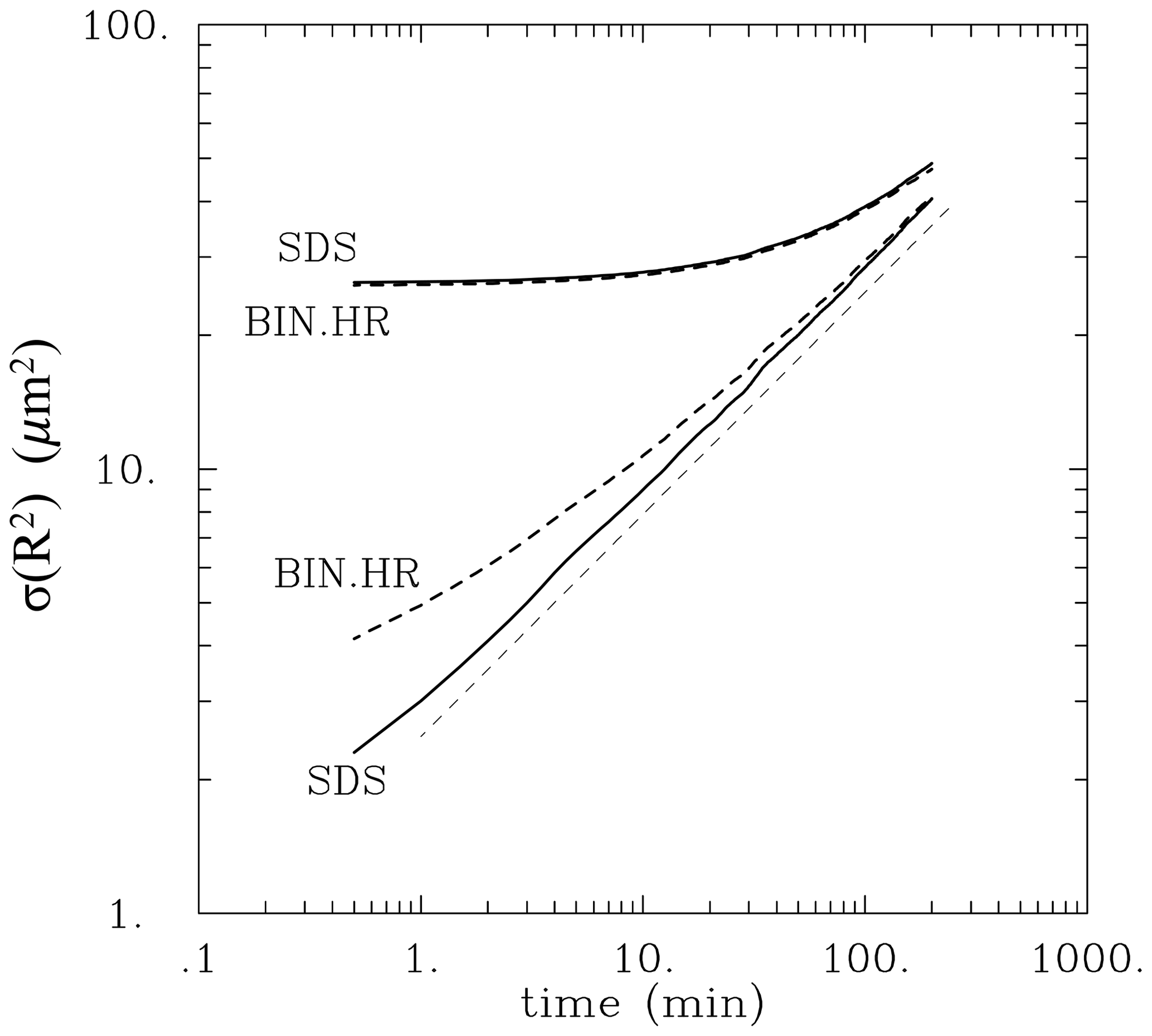
Figure A1Evolution of the radius-squared standard deviation for extended super-droplet (solid lines) and bin (dashed lines) simulations with 130 cm−3 droplet concentration and low TKE. The lower lines are for initially monodisperse simulations as in Figs. 6 (SDS) and 8 (BIN.HR) but extended from 20 to 200 min. The upper two lines are for simulations with truncated Gaussian initial droplet size distribution. Pale dashed line shows expected scaling.
To understand the results of the truncated Gaussian simulations, we show in Fig. A2 the droplet distributions at the onset of the simulations and after 10 min from the bin simulations. (Results from Lagrangian simulations are practically the same and thus they are not shown). When applying the linear vertical scale (Fig. A2a, c), the spectra look almost the same. However, panels with the logarithmic vertical scale show that the key change during the initial 10 min of the simulations is an expansion of the spectra into tails that are barely visible in panels a and c. Note that formation of the tails insignificantly affects the spectral width, which explains the evolutions shown in Fig. A1. The key point is that formation of the spectral tails beyond the truncated Gaussian initial distribution and transition to the increasing spectral width proceeds gradually and in virtually the same way in both Eulerian and Lagrangian simulations.
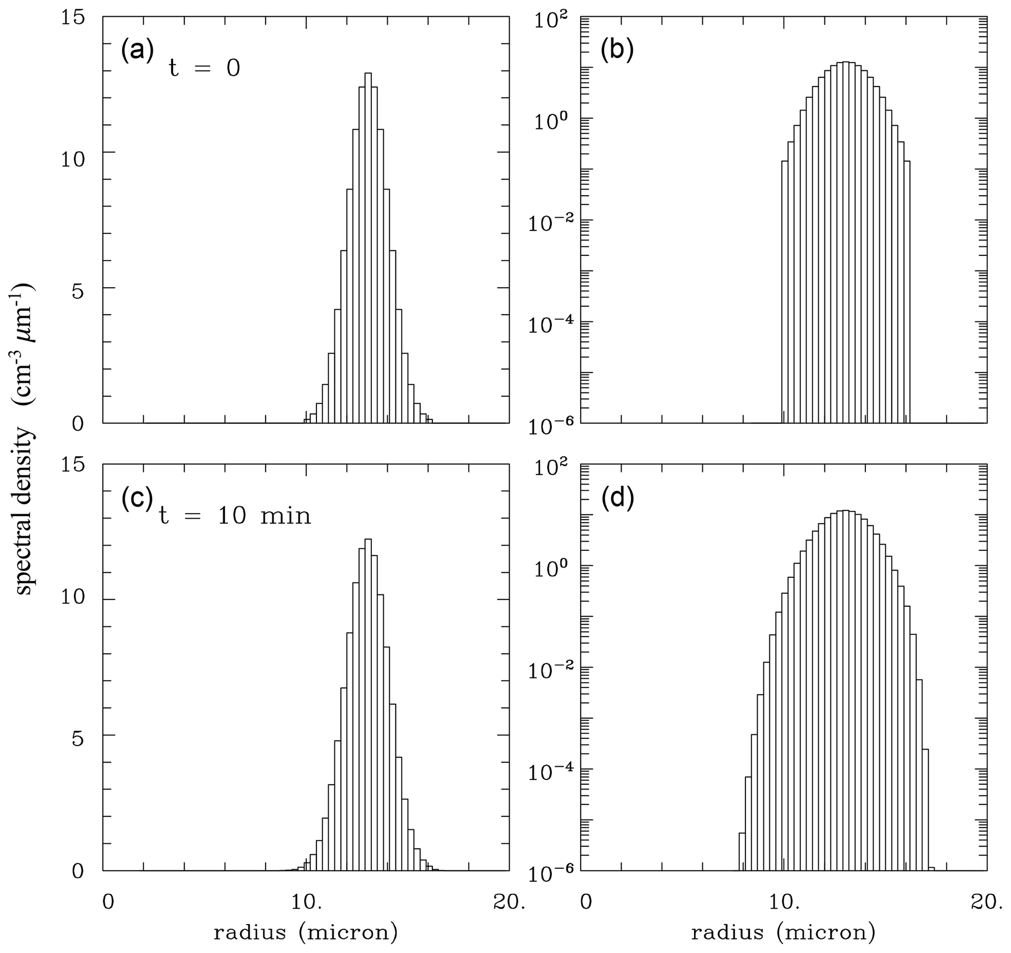
Figure A2Initial droplet spectra (a, b) and spectra at the time of 10 min (c, d) for bin simulations. Panels (a, c) and (b, d) show spectra using a linear and logarithmic vertical scale, respectively.
B1 Bin microphysics
The bin scheme solves the equation for the spectral density function , where dN(x) is the concentration of droplets at spatial location x and in the radius interval (rr+dr). Without droplet activation, sedimentation, and collisions, the continuity equation for ψ is
where u is the fluid velocity and is the diffusional droplet growth rate Eq. (9). In the discrete system consisting of N bins of droplet sizes, the spectral density function for each bin i with the radius r(i) is defined as , where N(i) is the concentration of droplets in the bin i and Δr(i) is the bin width. This transforms the continuous equation into a system of N coupled equations:
where the term on the right-hand side represents the condensational growth term, that is, the advective transport in radius space. It is calculated by combining all N bins at each grid volume as explained in the main text. The condensation rate Cd(x) is calculated as
where ρw=103 kg m−3 is the liquid water density.
B2 Super-droplets
The super-droplet scheme follows evolution in time and space of an ensemble of point particles that move with the flow and grow or evaporate in response to the grid-volume supersaturation. The evolution of the jth super-droplet position xj is calculated as
where u is the air flow velocity predicted by the dynamical model interpolated to the j super-droplet position. Each super-droplet responds to the grid-volume supersaturation and grows according to Eq. (9). The condensation rate is calculated as
where summation is over all super-droplets within a given grid volume, and rk and Nk are the kth super-droplet radius and multiplicity.
Data supporting this study are available at https://doi.org/10.5065/2ybq-nd09 (Grabowski, 2020c).
WWG developed the idea and ran the simulations. WWG and LT performed data analysis and prepared the paper.
The authors declare that they have no conflict of interest.
Simulations presented in this paper were completed in summer 2020 and the paper was drafted in summer and fall 2020 during NCAR's compulsory work-from-home period due to the COVID-19 pandemic. Initial flow data that were used to initiate the simulations were provided by JPL's Marcin Kurowski. Wojciech W. Grabowski acknowledges partial support from the U.S. DOE ASR Grant DE-SC0016476. NCAR is sponsored by the National Science Foundation.
This research has been partially supported by the U.S. DOE ASR Grant DE-SC0016476.
This paper was edited by Corinna Hoose and reviewed by two anonymous referees.
Andrejczuk, M., Grabowski, W. W., Malinowski, S. P., and Smolarkiewicz P. K.: Numerical simulation of cloud – clear air interfacial mixing, J. Atmos. Sci., 61, 1726–1739, 2004.
Andrejczuk, M., Reisner, J. M., Henson, B., Dubey, M. K., and Jeffery, C. A.: The potential impacts of pollution on a nondrizzling stratus deck: Does aerosol number matter more than type?, J. Geophys. Res., 113, D19204, https://doi.org/10.1029/2007JD009445, 2008.
Arabas, S. and Shima, S.-I.: Large-eddy simulations of trade wind cumuli using particle-based microphysics with Monte Carlo coalescence, J. Atmos. Sci., 70, 2768–2777, https:// doi.org/10.1175/JAS-D-12-0295.1, 2013.
Arabas, S., Jaruga, A., Pawlowska, H., and Grabowski, W. W.: libcloudph++ 1.0: a single-moment bulk, double-moment bulk, and particle-based warm-rain microphysics library in C++, Geosci. Model Dev., 8, 1677–1707, https://doi.org/10.5194/gmd-8-1677-2015, 2015.
Benmoshe, N., Pinsky, M., Pokrovsky, A., and Khain, A.: Turbulent effects on the microphysics and initiation of warm rain in deep convective clouds: 2-D simulations by a spectral mixed-phase microphysics cloud model, J. Geophys. Res., 117, D06220, https://doi.org/10.1029/2011JD016603, 2012.
Clark, T. L.: Numerical modeling of the dynamics and microphysics of warm cumulus convection, J. Atmos. Sci., 30, 857–878, 1973.
Dziekan, P., Waruszewski, M., and Pawlowska, H.: University of Warsaw Lagrangian Cloud Model (UWLCM) 1.0: a modern large-eddy simulation tool for warm cloud modeling with Lagrangian microphysics, Geosci. Model Dev., 12, 2587–2606, https://doi.org/10.5194/gmd-12-2587-2019, 2019.
Grabowski, W. W.: Separating physical impacts from natural variability using piggybacking technique, Adv. Geosci., 49, 105–111, https://doi.org/10.5194/adgeo-49-105-2019, 2019.
Grabowski, W. W.: Comparison of Eulerian bin and Lagrangian particle-based schemes in simulations of Pi Chamber dynamics and microphysics, J. Atmos. Sci., 77, 1151–1165, 2020a.
Grabowski, W. W.: Comparison of Eulerian bin and Lagrangian particle-based microphysics in simulations of nonprecipitating cumulus, J. Atmos. Sci., 77, 3951–3970, 2020b.
Grabowski, W. W.: Lagrangian and Eulerian droplets in DNS. Version 1.0. UCAR/NCAR – DASH Repository, https://doi.org/10.5065/2ybq-nd09, 2020c.
Grabowski, W. W. and Abade, G. C.: Broadening of cloud droplet spectra through eddy hopping: Turbulent adiabatic parcel simulations, J. Atmos. Sci., 74, 1485–1493, 2017.
Grabowski, W. W., Andrejczuk, M., and Wang, L.-P.: Droplet growth in a bin warm-rain scheme with Twomey CCN activation, Atmos. Res., 99, 290–301, 2011.
Grabowski, W. W., Dziekan, P., and Pawlowska, H.: Lagrangian condensation microphysics with Twomey CCN activation, Geosci. Model Dev., 11, 103–120, https://doi.org/10.5194/gmd-11-103-2018, 2018.
Grabowski, W. W., Morrison, H., Shima, S.-I., Abade, G. C., Dziekan, P., and Pawlowska, H.: Modeling of cloud microphysics: Can we do better?, B. Am. Meteorol. Soc., 100, 655–672, https://doi.org/10.1175/BAMS-D-18-0005.1, 2019.
Grinstein, F. F., Margolin, L. G., and Rider, W. J.: Implicit Large Eddy Simulation: Computing Turbulent Fluid Dynamics, Cambridge University Press, 2007.
Hoffmann, F., Yamaguchi, T., and Feingold, G.: Inhomogeneous mixing in Lagrangian cloud models: Effects on the production of precipitation embryos, J. Atmos. Sci., 76, 113–133, https://doi.org/10.1175/JAS-D-18-0087.1, 2019.
Khain, A. P., Beheng, K. D., Heymsfield, A., Korolev, A., Krichak, S. O., Levin, Z., Pinsky, M., Phillips, V., Prabhakaran, T., Teller, A., van den Heever, S. C., and Yano, J.-I.: Representation of microphysical processes in cloud-resolving models: Spectral (bin) microphysics versus bulk parameterization, Rev. Geophys., 53, 247–322, https://doi.org/10.1002/2014RG000468, 2015.
Kogan, Y. L.: The simulation of a convective cloud in a 3-D model with explicit microphysics. Part I: Model description and sensitivity experiments, J. Atmos. Sci., 48, 1160–1189, https://doi.org/10.1175/1520-0469(1991)048<1160:TSOACC>2.0.CO;2, 1991.
Lanotte, A. S., Seminara, A., and Toschi, F.: Cloud droplet growth by condensation in homogeneous isotropic turbulence, J. Atmos. Sci., 66, 1685–1697, 2009.
Lasher-Trapp, S. G., Cooper, W. A., and Blyth, A. M.: Broadening of droplet size distributions from entrainment and mixing in a cumulus cloud, Q. J. Roy. Meteor. Soc., 131, 195–220, https://doi.org/10.1256/qj.03.199, 2005.
Li, X.-Y., Brandenburg, A., Haugen, N. E. L., and Svensson, G.: Eulerian and Lagrangian approaches to multidimensional condensation and collection, J. Adv. Model. Earth Sy., 9, 1116–1137, https://doi.org/10.1002/2017MS000930, 2017.
Li, X.-Y., Svensson, G., Brandenburg, A., and Haugen, N. E. L.: Cloud-droplet growth due to supersaturation fluctuations in stratiform clouds, Atmos. Chem. Phys., 19, 639–648, https://doi.org/10.5194/acp-19-639-2019, 2019.
Margolin, L. G. and Rider, W. J.: A rationale for implicit turbulence modelling, Int. J. Numer. Meth. Fl., 39, 821–841, 2002.
Margolin, L. G., Rider, W. J., and Grinstein, F. F.: Modeling turbulent flow with implicit les, J. Turbul., 7, N15, https://doi.org/10.1080/14685240500331595, 2006.
Mordy, W.: Computations of the growth by condensation of a population of cloud droplets, Tellus, 11, 16–44, https://doi.org/10.1111/j.2153-3490.1959.tb00003.x, 1959.
Morrison, H., Witte, M., Bryan, G. H., Harrington, J. Y., and Lebo, Z. J.: Broadening of modeled cloud droplet spectra using bin microphysics in an Eulerian spatial domain. J. Atmos. Sci., 75, 4005–4030, https://doi.org/10.1175/JAS-D-18-0055.1, 2018.
Onishi, R., Baba, Y., and Takahashi, K.: Large-scale forcing with less communication in finite-difference simulations of stationary isotropic turbulence, J. Comp. Phys., 230, 4088–4099, 2011.
Riechelmann, T., Noh, Y., and Raasch, S.: A new method for large-eddy simulations of clouds with Lagrangian droplets including the effects of turbulent collision, New J. Phys., 14, 065008, https://doi.org/10.1088/1367-2630/14/6/065008, 2012.
Rosales, C. and Meneveau, C.: Linear forcing in numerical simulations of isotropic turbulence: Physical space implementations and convergence properties, Phys. Fluids., 17, 095106, https://doi.org/10.1063/1.2047568, 2005.
Sardina, G., Picano, F., Brandt, L., and Caballero, R.: Continuous growth of droplet size variance due to condensation in turbulent clouds, Phys. Rev. Lett., 115, 184501, https://doi.org/10.1103/PhysRevLett.115.184501, 2015.
Shima, S.-I., Kusano, K., Kawano, A., Sugiyama, T., and Kawahara, S.: The superdroplet method for the numerical simulation of clouds and precipitation: A particle-based and probabilistic microphysics model coupled with a non-hydrostatic model, Q. J. Roy. Meteor. Soc., 135, 1307–1320, https://doi.org/10.1002/qj.441, 2009.
Siebert, H., Lehmann, K., and Wendisch, M.: Observations of small-Scale turbulence and energy dissipation rates in the cloudy boundary layer, J. Atmos. Sci., 63, 1451–1466, 2006.
Siebesma, A. P., Bretherton, C. S., Brown, A., Chlond, A., Cuxart, J., Duynkerke, P. G., Jiang, H., Khairoutdinov, M., Lewellen, D., Moeng, C. H., Sanchez, E., Bjorn Stevens, B., and Stevens, D. E.: A large eddy simulation intercomparison study of shallow cumulus convection, J. Atmos. Sci., 60, 1201–1219, https://doi.org/10.1175/1520-0469(2003)60<1201:ALESIS>2.0.CO;2, 2003.
Stevens, B., Moeng, C. H., Ackerman, A. S., Bretherton, C. S., Chlond, A., de Roode, S., Edwards, J., Golaz, J. C., Jiang, H., Khairoutdinov, M., Kirkpatrick, M. P., Lewellen, D. C., Lock, A., Müller, F., Stevens, D. E., Whelan, E., and Zhu, P.: Evaluation of large-eddy simulations via observations of nocturnal marine stratocumulus, Mon. Weather Rev., 133, 1443–1462, 2005.
Thomas, L., Grabowski, W. W., and Kumar, B.: Diffusional growth of cloud droplets in homogeneous isotropic turbulence: DNS, scaled-up DNS, and stochastic model, Atmos. Chem. Phys., 20, 9087–9100, https://doi.org/10.5194/acp-20-9087-2020, 2020.
Unterstrasser, S., Hoffmann, F., and Lerch, M.: Collection/aggregation algorithms in Lagrangian cloud microphysical models: rigorous evaluation in box model simulations, Geosci. Model Dev., 10, 1521–1548, https://doi.org/10.5194/gmd-10-1521-2017, 2017.
Vaillancourt, P., Yau, M. K., and Grabowski, W. W.: Microscopic approach to cloud droplet growth by condensation. Part I: Model description and results without turbulence, J. Atmos. Sci., 58, 1945–1964, 2001.
Vaillancourt, P. A., Yau, M. K., Bartello, P., and Grabowski, W. W.: Microscopic approach to cloud droplet growth by condensation. Part II: Turbulence, clustering and condensational growth, J. Atmos. Sci., 59, 3421–3435, 2002.
vanZanten, M. C., Stevens, B., Nuijens, L., Siebesma, A. P., Ackerman, A. S., Burnet, F., Cheng, A., Couvreux, F., Jiang, H., Khairoutdinov, M., Kogan, Y., Lewellen, D. C., Mechem, D., Nakamura, K., Noda, A., Shipway, B. J., Slawinska, J., Wang, S., and Wyszogrodzki, A.: Controls on precipitation and cloudiness in simulations of trade-wind cumulus as observed during RICO, J. Adv. Model. Earth Sy., 3, M06001, https://doi.org/10.1029/2011MS000056, 2011.
- Abstract
- Introduction
- Homogeneous isotropic turbulence simulations
- Thermodynamics in ILES moist simulations
- ILES moist simulations with droplets
- Results
- Grid-volume by grid-volume analysis of macro- and microphysical properties
- Summary and conclusions
- Appendix A: The impact of initial conditions
- Appendix B: Summary of Eulerian and Lagrangian microphysics equations
- Data availability
- Author contributions
- Competing interests
- Acknowledgements
- Financial support
- Review statement
- References