the Creative Commons Attribution 4.0 License.
the Creative Commons Attribution 4.0 License.
 | 17 Mar 2021
Identifying forecast uncertainties for biogenic gases in the Po Valley related to model configuration in EURAD-IM during PEGASOS 2012
Hendrik Elbern
Forecasts of biogenic trace gases in the planetary boundary layer (PBL) are highly affected by simulated emission and transport processes. The Po region during the PEGASOS campaign in summer 2012 provides challenging, yet common, conditions for simulating biogenic gases in the PBL. This study identifies and quantifies principal sources of forecast uncertainties induced by various model configurations under these conditions. Specifically, the effects of model configuration on different processes affecting atmospheric distributions of biogenic trace gas distributions are analyzed based on a priori available information. The investigation is based on the EURopean Air pollution Dispersion – Inverse Model (EURAD-IM) chemistry transport model employing the Model for Emissions of Gases and Aerosols from Nature version 2.1 (MEGAN 2.1) biogenic emission module and Regional Atmospheric Chemistry Mechanism – Mainz Isoprene Mechanism (RACM-MIM) as the gas phase chemistry mechanism. Two major sources of forecast uncertainties are identified in this study. Firstly, biogenic emissions appear to be exceptionally sensitive to land surface properties inducing total variations in local concentrations of up to 1 order of magnitude. Moreover, these sensitivities are found to be highly similar for different gases and almost constant during the campaign, varying only diurnally. Secondly, the model configuration also highly influences regional flow patterns with significant effects on pollutant transport and mixing. This effect was corroborated by diverging source regions of a representative air mass and thus applies also to non-biogenic gases. As a result, large sensitivities to model configuration are found for surface concentrations of isoprene, as well as OH, affecting reactive atmospheric chemistry. Especially in areas with small-scale emission patterns, changes in the model configuration are able to induce significantly different local concentrations. The amount and complexity of sensitivities found in this study demonstrate the need to consider forecast uncertainties in chemical transport models with a special focus on biogenic emissions and pollutant transport.
- Article
(21853 KB) - Full-text XML
- BibTeX
- EndNote


One of the major challenges in tropospheric chemistry modeling is the skillful simulation of biogenic compounds, comprising emissions, atmospheric transport, chemical reactions and deposition. Being actively evolved in the formation of secondary organic aerosol (SOA; e.g., Geng et al., 2011; Shrivastava et al., 2017) and the photochemical production of tropospheric ozone (e.g., Geng et al., 2011; Wu et al., 2015), biogenic volatile organic compounds (BVOCs) have a significant impact on trace gas and aerosol composition. However, important BVOCs like isoprene show a large spatiotemporal variability which hampers the investigation of regional to global effects (e.g., Mentel et al., 2013). As biogenic emissions are dependent on various environmental conditions, forecasts of biogenic gases are exceptionally sensitive to the model setup, e.g., parameters and input fields.
Emili et al. (2016) claim that an investigation of major sources of forecast uncertainties is required before forecast errors can be estimated. Generally, atmospheric chemical forecasts are highly affected by a large number of model inputs and parameters, including the meteorological forcing. In this regard, Zhang et al. (2012b) state that more effort is needed to find how meteorology and model setup affect chemical forecasts. Chemistry transport models (CTMs) are driven by numerical weather prediction (NWP) forecasts and thus inherit their errors. Different meteorological input from different NWP models or different setups of the NWP model are found to influence chemical forecasts significantly (e.g., Hu et al., 2010; Zhang et al., 2012a; Vogel et al., 2020). In addition, CTMs are sensitive to information on the earth's surface type and vegetation distribution, as well as emission maps (e.g., Ma and van Aardenne, 2004; Chen et al., 2014). The formulation of aerosol uptake and reactive chemistry may also serve as important components of the model configurations (e.g., Zhang et al., 2012c; Gama et al., 2019; Chen et al., 2019).
Concerning biogenic gases, highly complex dependencies of the emission process induce exceptionally large sensitivities to various model configurations, including land use information and meteorological conditions (e.g., Wang et al., 2017; Henrot et al., 2017). These complex dependencies result in large differences in modeled biogenic emissions on a global scale. Focusing on climate-related dependencies, Arneth et al. (2011) investigated global annual changes in modeled isoprene emissions due to climatology and vegetation input. Although the authors identified substantial effects of model input on globally averaged emissions, their results indicated increased sensitivity and complexity on smaller scales.
On regional and local scales, modeled trace gas distributions are increasingly influenced by boundary layer dynamics which control advection and the mixing of air masses (e.g., Eder et al., 2006; Zhang et al., 2012b; Banks et al., 2016). An example of highly complex chemistry–turbulence interactions is found in Kaser et al. (2015), which investigated effects of the local separation of isoprene and OH. The large spatiotemporal gradients of observed biogenic gases make regional forecasts highly sensitive to both local emissions and flow patterns. Furthermore, a forecast evaluation of biogenic gases is limited by exceptionally sparse observations suitable for comparison with CTM forecasts (e.g., Arneth et al., 2008; Guenther et al., 2012). This is more the case as available in situ observations of BVOCs are hardly representative of an area larger than a few kilometers which is numerically resolved by CTMs. Ideally though hardly available, free boundary layer probing under well-mixed conditions may allow for reliable model evaluation.
In summer 2012, high-resolution observations of chemical distributions in the planetary boundary layer (PBL) were performed in the Po Valley during the PEGASOS campaign (Pan-European Gas-AeroSOls-climate interaction Study). The Po Valley is known to be one of the most polluted regions in Europe (e.g., Sogacheva et al., 2007; Israelevich et al., 2012; Finardi et al., 2014; Kontkanen et al., 2016; Sandrini et al., 2016). Firstly, this region is highly populated (Finardi et al., 2014) with accordingly high anthropogenic emissions from traffic, industry and power plants (e.g., Kontkanen et al., 2016). Emission hotspots in urban areas like Bologna and Modena are surrounded by agricultural areas with various emission characteristics. Moreover, heterogeneous and highly patchy agricultural surface patterns are likely to remain unresolved in regional models with some kilometers of grid spacing. Secondly, the topography of the Po Valley impedes the mixing and exchange of polluted air masses on a regional scale (e.g., Sogacheva et al., 2007). This is mainly due to the Alps in the north and west and the Apennine Mountains in the southwest framing the valley on three sides. The inner Po Valley is characterized by a flat topography supporting the development of nocturnal inversion layers during cloud-free nights (Li et al., 2014). Thus, the Po Valley is expected to provide challenging conditions with respect to local emission patterns and regional transport processes.
In the framework of the PEGASOS Po Valley campaign 2010, a number of studies focus on in situ observations of aerosol composition (e.g., Wolf et al., 2015; Sullivan et al., 2016; Kontkanen et al., 2016; Rosati et al., 2016b; Bucci et al., 2018; Karnezi et al., 2018). Some findings point towards potential difficulties in simulating low-level transport and biogenic gases in this region. According to Wolf et al. (2015) and Rinaldi et al. (2015), different local transport patterns affected observed aerosol composition in this region. Rosati et al. (2016a) found different aerosol properties in distinct coexisting layers within the evolving morning boundary layer. Regarding BVOCs, Kaiser et al. (2015) observed low concentrations in the Po Valley during the campaign. Additionally, Karnezi et al. (2018) found that the largest variation in simulated overall SOA during the campaign was induced by biogenic SOA components. Overall a dedicated quantitative assessment study on forecast uncertainties of biogenic trace gases prior to SOA and ozone formation is as yet missing.
In this context, airborne observations from the PEGASOS campaign allow for a detailed evaluation of simulated biogenic gases. However, effects of individual model configurations on forecasts should be taken into account when evaluating the forecast model and estimating related uncertainties. The main goal of this study is to identify and quantify principal sources of forecast uncertainties by evaluating the effects of different model configurations on atmospheric chemical processes. Here, the evaluation does not refer to a quantitative forecast evaluation with respect to observations. Instead we aim to analyze the pathways of the simulated differences in order to better understand their impact. With this approach, differences in simulated concentrations can be traced back to specific model configuration options affecting different parts of the modeling system. Thus, this study provides a precursory step prior to comprehensive forecast validation by observations, as well as probabilistic simulations. Focusing on biogenic gases, various kinds of sensitivities related to model input and setup are considered, including the configuration of the meteorological model. Other potential sources of uncertainties related to chemical conversions are not investigated in this study.
Section 2 gives an overview of the context of this study, including the meteorological situation during the campaign and the selection of specific cases. The modeling system and important model configurations are described in Sect. 3. The evaluation of sources of forecast uncertainties in the Po Valley during the PEGASOS campaign in 2012 is performed in two steps. Firstly, effects of model configurations on biogenic emissions, pollutant transport and dry deposition are analyzed (Sect. 4). In the context of pollutant transport, calculating source areas of air masses allows for a detailed analysis of modeled air mass history with respect to transport and mixing processes. Secondly, the effects of these model processes are analyzed in terms of differences in local trace gas concentrations (Sect. 5).
The results focus on a set of biogenic gases with different dependencies on the model processes to demonstrate differences and similarities between gases. Isoprene is a directly emitted BVOC with a comparably short atmospheric lifetime. Methanol is part of the model variable “HC3” which also includes ethanol and propane as non-biogenically emitted alkanes. The model variable “aldehyde” represents a composite of oxidized BVOCs which are affected by several processes, including biogenic and anthropogenic emissions, photochemical production, atmospheric transport, and dry deposition. Detailed results in Sects. 4 and 5 are given for a single case on 12 July 2012. Introducing dominant uncertainties to the model, generalized sensitivities of biogenic emissions during the campaign are presented in Sect. 6. Finally, Sect. 7 evaluates the effects of different model configurations and concludes consequences for model evaluation and uncertainty estimation.
The PEGASOS campaign in the Po Valley took place from 18 June to 13 July 2012. A Zeppelin NT (new technology) served as airborne observational platform sampling the PBL during 22 flights over the Po Valley. Detailed documentation of the zeppelin's measurement configurations during the campaigns in 2012 is available from Jäger (2013). Section 2.1 gives a short overview of the synoptic-scale meteorological conditions during the campaign. The averaged daily evolution of local meteorological quantities observed at San Pietro Capofiume (SPC) during the campaign is given in Kontkanen et al. (2016). Specific cases which are identified to be representative for this study are described in Sect. 2.2.
2.1 Meteorological conditions
During June and July 2012, the synoptic situation in Europe was influenced by Rossby wave activity, as shown in Fig. 1. Eastward-moving troughs forced several low-pressure systems to move across central and northern Europe. Nevertheless, the weather in the Po Valley was continuously influenced by southern high-pressure systems.

Figure 1Geopotential height at 500 hPa (color coded+isolines) and horizontal winds at 2 km height (arrows) during the PEGASOS campaign in the Po Valley as simulated by WRF (initialized with IFS reanalysis; setup denoted as “reference” later on).
At the very beginning of the campaign, a large trough over the Atlantic Ocean induced southwesterly flow over Europe. The trough detached from the polar vortex and moved northeastwards towards southern Sweden during the next days. On 25 June 2012, large pressure gradients between this low-pressure system and a high-pressure system over the Strait of Gibraltar forced strong northwesterly to westerly winds over central Europe (Fig. 1a). Under these conditions, the Alps act as an orographic barrier resulting in low wind speeds in the leeward Po Valley. These calm conditions are confirmed by a radio sounding in SPC from the Italian Meteorological Service (Servizio Meteorologico). During the next days, the low- and high-pressure systems weakened and moved eastwards towards the Black Sea. On 1 July 2012, a trough extended from the British Isles towards Spain, causing southwesterly flow over central Europe (Fig. 1b). The trough was connected to several surface lows and frontal activity inducing cloudy and rainy conditions from Spain to Poland and Finland. Being separated by the Alps, the weather in northern Italy was still influenced by the weakened high-pressure system in the east. Thus, clear and partly foggy conditions with calm winds and temperatures above 20 ∘C were observed in the Po Valley during the morning hours on 1 July 2012.
The trough and its controlling low-pressure systems propagated to the northeast during the next days. Subsequently, a cutoff low developed south of Iceland and started to separate from the polar vortex on 4 July 2012. Three days later, on 7 July 2012, the center of the cutoff low was located over the British Isles (Fig. 1c). Again, a cold front over Poland influenced the local weather north of the Alps but did not affect the Po region. Instead, slow varying winds from southwestern to northwestern directions and clear sky conditions were still observed in the Po Valley by the Italian Meteorological Service. These conditions in the Po Valley persisted until the end of the campaign on 13 July 2012. During this time, the cutoff low weakened and reconnected with the polar vortex. On 12 July 2012, a new trough was formed and moved towards the North Sea (Fig. 1d) along with a sequence of associated surface lows. Additionally, a large high-pressure system formed over northwestern Africa which directed westerly flow towards southwestern Europe.
Radiosonde observations at SPC from the Italian Meteorological Service are launched at 00:00 UTC each day. On 12 July 2012, the sounding states calm conditions with westerly winds of about 1.5 to 5 m s−1 in the lowest 100 m. The temperature at 00:00 UTC was 21.2 ∘C close to the surface with a temperature inversion reaching up to 26.8 ∘C at 200 m height. At this time, the relative humidity reduces steadily from 69 % to 42 % at about 1 km height. These local conditions are sufficiently well simulated by the Weather Research and Forecasting (WRF) forecasts for all model configurations used in this study at 00:00 UTC. Simulated near-surface winds are between 2.5 and 5.5 m s−1 from southwestern directions, relative humidity close to the surface ranges from 50 % to 69 %, and temperatures vary between 21.3 and 24.6 ∘C. All simulations capture the inversion but tend to underestimate its intensity as maximum temperatures at 200 m height are about 25 ∘C.
2.2 Selected cases
The set of observational instruments on board the zeppelin was deployed following the emphasis assigned to each individual PEGASOS flight (see, e.g., Jäger, 2013, for an overview). Flight patterns are either vertical profiles by helical flight patterns close to the base station at SPC or horizontal transects to different parts of the Po Valley. Flight number F049 on 12 July 2012 is an example for a helical flight pattern which was performed close to Argenta. With a radius of about 1 km, the zeppelin spanned altitudes from 50 up to 750 m above ground between 03:20 and 09:20 UTC. In contrast, horizontal transects were performed to the central Po Valley and the Adriatic Sea, as well as the Apennine Mountains. During some of the flights to the Apennine Mountains – like flight number F039 on 1 July 2012 – the zeppelin followed a large valley towards Monte Cimone (2165 m a.s.l., above sea level). Most of the flights took place in the early morning hours to investigate the morning development of the mixed boundary layer. On 7 July 2012 only, flight number F045 was scheduled between 17:00 and 20:20 UTC to investigate effects of the weakening vertical mixing during the evening hours.
This study focuses on three different cases during the PEGASOS Po Valley campaign: (1) early morning on 1 July 2012, (2) evening on 7 July 2012 and (3) early morning on 12 July 2012. The selection is made on the differences in synoptic conditions, time of day and flight pattern in order to cover different principal conditions during the campaign. Thus, these cases allow for a generalized analysis of averaged sensitivities in the Po Valley during the campaign. From these, special emphasis is placed on the early morning hours on 12 July 2012, which has already been selected for other studies (Li et al., 2014; Kaiser et al., 2015). It appears to be a typical case for investigating chemical components during the development of a morning mixed layer during this campaign.
The atmospheric chemical simulations are performed by the EURopean Air pollution Dispersion – Inverse Model (EURAD-IM) modeling system, which will be introduced in Sect. 3.2. As the meteorological simulation provides an important set of model inputs, the numerical weather prediction model WRF serving as the meteorological driver for EURAD-IM is shortly described in Sect. 3.1. Finally, Sect. 3.3 describes the selected model inputs and configurations which are considered during this study. For all selected cases, the simulations of WRF and EURAD-IM are each initialized 1 d before the day of evaluation at 00:00 UTC. Thus, at least 27 h of spin-up is performed for all meteorological and chemical fields in addition to the initialization of meteorological fields, including soil moisture in WRF. Both models share the same domain and projection, which is Lambert conformal with 15 km horizontal spacing (compare Fig. 1). Based on this, a 5 km and the final 1 km domains are driven by initial and boundary conditions from their respective mother domains. The vertical layers are defined by terrain-following σ coordinates with 23 levels extending up to 100 hPa for both models.
3.1 WRF numerical weather prediction
The WRF (Weather Research and Forecasting) model is a mesoscale numerical weather prediction model devised by a joint coordination effort of NCAR (National Center for Atmospheric Research), NOAA (National Oceanic and Atmospheric Administration), the US Air Force, the Naval Research Laboratory, the University of Oklahoma and the Federal Aviation Administration. In this study, the advanced research WRF (WRF-ARW) version 3.8.1 is used (Skamarock et al., 2008). WRF-ARW solves a fully compressible non-hydrostatic formulation of the prognostic equations. Time integration is performed by second- or third-order Runge–Kutta schemes. The vertical grid is defined by terrain-following hydrostatic pressure coordinates, and the prognostic variables are horizontally staggered in an Arakawa C-grid (Arakawa and Lamb, 1977) stencil. For a detailed description of WRF-ARW 3.8.1, see Skamarock et al. (2008).
Multiple schemes for various kinds of parameterizations are implemented in WRF-ARW. Available parameterizations account for subgrid-scale processes related to the boundary and surface layer (SL), land and urban surface, lake physics, short- and long-wave radiation, cloud microphysics, and cumulus parameterizations. Effects of these parameterizations on atmospheric chemical forecasts are investigated in this study. The selection of parameterization schemes is given in Sect. 3.3. A detailed description of the available parameterization schemes can be found in Skamarock et al. (2008).
3.2 EURAD-IM chemistry transport model
The atmospheric chemical data assimilation system EURAD-IM (EURopean Air pollution Dispersion – Inverse Model) combines a state-of-the-art chemistry transport model with spatiotemporal data assimilation and inversion methods (Elbern et al., 2007). The chemistry transport model within EURAD-IM provides forecasts of a large set of gas phase and aerosol compounds up to lower stratospheric levels (e.g., Hass et al., 1995). Considered transformation processes include dynamical transformations due to advective and diffusive processes, as well as reactive chemistry with other compounds and photolysis. For this study, the RACM-MIM (Regional Atmospheric Chemistry Mechanism – Mainz Isoprene Mechanism; Geiger et al., 2003) for reactive chemistry is selected, which considers 221 chemical and 23 photolysis reactions of 84 gases, including condensed isoprene degradation (MIM; Pöschl et al., 2000).
Emissions from anthropogenic and biogenic sources are treated separately, for which anthropogenic emissions are provided by the TNO-MACC-II inventory (Kuenen et al., 2014). The MEGAN 2.1 (Model for Emissions of Gases and Aerosols from Nature version 2.1; Guenther et al., 2012) module is used for biogenic emissions from urban, natural and agricultural sources. In total, 147 chemical compounds are considered which are grouped into 19 classes according to their emission properties. For each of these component classes, vegetation-dependent emissions are calculated from standard emissions multiplied by the local vegetation fraction. These vegetation-dependent emissions are scaled by an activity factor to account for variations in the environmental conditions. According to Guenther et al. (2012), effects of radiation, temperature, leaf age, soil moisture and CO2 are included in a multiplicative manner. Therefore, required input parameters include fields of plant functional types (PFTs), leaf area index (LAI), solar radiation, air temperature and soil moisture.
Dry and wet deposition is implemented in the model, in which wet deposition is included in the treatment of clouds. The dry deposition velocity is modeled by a multiple path resistance scheme according to Zhang et al. (2003), in which aerodynamic resistance and quasi-laminar sublayer resistance are a function of friction velocity (Wesely et al., 2002). In addition, different contributions to the overall canopy resistance depend on photosynthetically active radiation, air temperature, water-vapor deficit, LAI and friction velocity.
The EURAD-IM system includes 4-dimensional variational data assimilation (4Dvar) for initial state and emission rate optimization (Elbern et al., 2007). This assimilation algorithm comprises an adjoint model which integrates a signal backward in time. Being implemented into the modeling system, the adjoint model can be modified to quantify the history of selected air masses according to Vogel et al. (2020). By switching off chemical conversions, the retroplume operator allows for the identification and investigation of source regions of air parcels, including the convolution and mixing of different air masses.
3.3 Model inputs
In the following, important model configurations and their realizations selected in this study are briefly described. As summarized in Table 1, two representative realizations – a reference and an alternative option – are selected for each model configuration. Most model configurations apply the meteorological forecasts of WRF and transfer to the atmospheric chemical forecasts via its dependencies on meteorological conditions. Firstly, initial and boundary conditions for WRF are provided by global meteorological analyses. Here the IFS reanalysis (Hortal, 1998) provided by ECMWF is used as reference, and the operational Global Forecast System (GFS) analysis from NOAA (Caplan et al., 1997) serves as an alternative option.
Table 1Selection and description of considered model input sources. PX signifies Pleim–Xiu surface layer parameterization, and Du signifies Dudhia short-wave radiation parameterization. For further information on parameterization schemes in WRF, see, e.g., Skamarock et al. (2008). Increased roughness lengths are based on Berndt (2018).
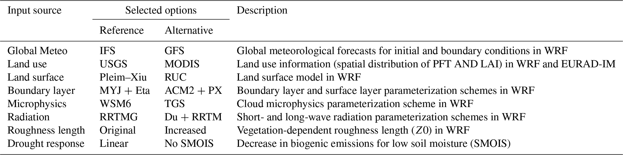
Secondly, reference information on land surface and vegetation types are given in the form of USGS (US Geological Survey) land use categories. In WRF, this land use information is provided by the GLCC (Global Land Cover Characteristics) database. Based on AVHRR (Advanced Very High Resolution Radiometer) observations between April 1992 and March 1993, the surface at each location is classified as a single USGS land use category (Loveland et al., 2000). The USGS database includes 24 different categories, including water, urban, snow and ice, as well as various vegetative surface categories (Anderson et al., 1976). Although the database provides unsupervised surface classifications, the occurrence of different surface types is treated by mixed categories (e.g., “Cropland/Woodland Mosaic”). Vegetation products from MODIS and Sentinel-2 satellites can give more recent information on spatial distributions and also the temporal evolution of vegetation types. Currently, Sentinel-2 provides vegetation products in the highest resolution (up to 10 m horizontal resolution; e.g., Immitzer et al., 2016; Drusch et al., 2012). However, these data are not available for 2012 as the satellite was launched in 2015.
Thus, fractional vegetation data with 1 km spatial resolution based on MODIS (MODerate-resolution Imaging Spectroradiometer; Friedl et al., 2002) observations are transferred to land use information for this study. Multiple studies indicate a more detailed and reliable characterization compared to AVHRR-based products (e.g., Hansen et al., 2002; Smirnova et al., 2016). However, GLCC land use information provides a basically different data set which has been used in a great number of studies over the last decades until today (e.g., Krinner et al., 2005; Dee et al., 2011; Sellar et al., 2019). Thus, using GLCC data from USGS as the reference option provides a solid basis for investigating changes in land use information induced by MODIS. Transferring MODIS data to land use categories requires additional information on urban areas, water, snow and ice. Assuming an appropriate representation of these basic surface types, the related information of USGS was also used in the MODIS-based classification. If the MODIS categories do not sum up to 100 %, the missing fraction is defined according to the USGS land use categories if they are not zero.
Thirdly, WRF offers various options for different kinds of parameterizations. For this study, sensitivities to the land surface model (LSM), boundary and surface layer parameterizations and cloud microphysics parameterizations, as well as short- and long-wave radiation parameterizations, are considered. The selection of parameterization schemes is based on the frequency of usage (according to https://www2.mmm.ucar.edu/wrf/users/wrf_physics_survey.pdf, last access: 6 April 2020) and differences in the underlying approach. For example, the two layer Pleim–Xiu (Pleim and Xiu, 1995; Xiu and Pleim, 2001) and the multi-layer RUC (rapid update cycle; Benjamin et al., 2004) schemes serve as references and alternative options for LSM. The MYJ (Mellor–Yamada–Janjić; Janjic, 1994) and ACM2 (Asymmetric Convection Model version 2; Pleim, 2007) boundary layer parameterizations are selected because of their 1.5-order local and 1st-order non-local approaches, respectively. As boundary and surface layer parameterizations are closely related, the Eta-similarity (Janjic, 1996) and Pleim–Xiu (Pleim, 2006) surface layer parameterizations are selected with respect to the boundary layer parameterizations, and resulting effects are investigated together. For cloud microphysics, the WSM6 (WRF Single-Moment 6-class; Hong and Lim, 2006) and TGS (Thompson graupel scheme; Thompson et al., 2008) parameterizations are selected. A RRTMG (rapid radiative transfer model for general circulation models; Iacono et al., 2008) scheme is used as reference for short- and long-wave radiation, while alternative options are Dudhia (Dudhia, 1989) and a RRTM (rapid radiative transfer model; Mlawer et al., 1997), respectively. No effect of cumulus parameterization schemes is investigated here because the parameterization is switched off as the 1 km domain is assumed to resolve related processes.
Finally, one additional model configuration is considered for pollutant transport and dry deposition, as well as biogenic emissions. The effect of drought response to biogenic emissions introduces an important source of uncertainty. No response to soil moisture is implemented in the MEGAN 2.1 code (http://lar.wsu.edu/megan/docs/meganv2.10_beta.tar.gz, last access: 9 July 2018), but Guenther et al. (2012) propose a linear reduction of isoprene emissions below a soil moisture threshold. While a general reduction in biogenic emissions under dry conditions is indicated by multiple studies, the explicit dependency of emitted gases is still under discussion (e.g., Pegoraro et al., 2004; Lavoir et al., 2009; Wu et al., 2015). Recently, Jiang et al. (2018) formulated drought response in the subsequent version (MEGAN 3) as a function of photosynthesis and generalized water stress. In this study, the linear decrease in emissions proposed by Guenther et al. (2012) is implemented as reference for all biogenic gases, while no dependency is assumed as an alternative option (“no SMOIS”). Regarding transport, Berndt (2018) indicates that predefined values of roughness length in WRF underestimate true roughness in Europe. Thus for pollutant transport and dry deposition, effects of increased vegetation-dependent roughness lengths are investigated based to the values used by Berndt (2018).
Effects of different types of model inputs and configurations are investigated for biogenic emissions (Sect. 4.1), dry deposition velocities (Sect. 4.2) and pollutant transport (Sect. 4.3). This section focuses on the results for 12 July 2012, which are discussed in more detail. All three model processes discussed here are highly dependent on meteorological fields. However, using an existing meteorological ensemble appears to be not sufficient for this application. An investigation of sensitivities from the Global Forecast System (GFS) ensemble from NOAA did not induce significant differences in the simulated boundary layer in this case (not shown).
4.1 Effects on biogenic emissions
The effects of model configurations on biogenic emissions of different gases are given in Figs. 2 and 3. As the changes induced by the different model configurations are similar for all presented biogenic gases, the following description focuses on isoprene and HC3 shown in Fig. 2. Note that biogenic HC3 emissions refer solely to methanol which is the only biogenically emitted compound in this chemical group defined in the model.
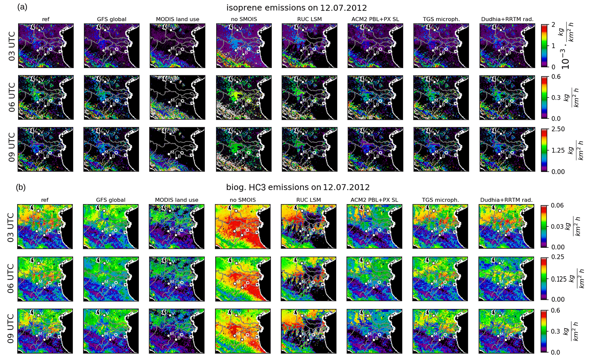
Figure 2Isoprene (a) and biogenic HC3 (b) emissions on 12 July 2012 at 03:00, 06:00 and 09:00 UTC (coded by color) for different model configurations: reference, GFS global meteorology, MODIS land use, no response to soil dryness (no SMOIS), RUC LSM, ACM2 boundary layer plus Pleim–Xiu surface layer schemes, TGS microphysics, and Dudhia short-wave plus RRTM long-wave radiation. Some important cities (Verona, Bologna, Modena) are indicated by their initial letters. The location of the zeppelin's observations on this day is given as a small circle.

Figure 3The α-pinene (a), limonene (b), biogenic ethene (c) and biogenic aldehyde (d) emissions on 12 July 2012 at 03:00, 06:00 and 09:00 UTC (coded by color) for different model configurations. Plotting conventions are like in Fig. 2.
Differences between nighttime (03:00 UTC) and daytime (09:00 UTC) emissions are more significant for isoprene than for other biogenic gases. This is because isoprene is a direct product of photosynthesis which is mainly limited to daytime conditions. For the reference setup (“ref”), daytime isoprene emissions are mainly restricted to the Apennine Mountains and two areas within the central Po Valley north of Modena and Bologna. According to USGS land use, these locations are assigned as “Deciduous Broadleaf Forest” and “Crop/Woodland Mosaic”, respectively. In contrast to “Dryland Cropland and Pasture” in the rest of the valley, broadleaf trees emit high levels of isoprene. Thus, even small numbers of trees result in significantly increased local isoprene emissions. Biogenic emissions of α-pinene, limonene and aldehyde are also increased in these regions but with decreasing characteristics. In contrast, biogenic emissions of methanol and aldehydes are almost equally emitted by all vegetation types in this regions. This results in a comparably uniform distribution over most parts of the domain with a significant reduction in the Apennine Mountains.
The high dependency on tree coverage is emphasized by comparing reference biogenic emissions to emissions based on MODIS land use (“land use”). In contrast to USGS, MODIS does not indicate any trees within the Po Valley, which results in negligible biogenic emissions in this region. Although this effect is most prominent for isoprene, significant emission reduction is found for all considered biogenic gases. At the same time, the whole Apennine Mountains and southern foothills of the Alps are assigned as having a high coverage of broadleaf trees resulting in high isoprene emissions. The use of GFS global meteorology does not change the general emission patterns (“global”). Caused by different initial and boundary conditions, all biogenic emissions are slightly reduced in the whole region. The implemented response of biogenic emissions to soil dryness significantly influences biogenic emissions (no SMOIS). By neglecting this response, emissions are considerably larger than for the reference case, especially in the southern part of the domain. As soil moisture decreases after sunrise, the largest sensitivities are found at 09:00 UTC for both gases.
The RUC LSM induces slightly increased biogenic emissions of all considered gases in most areas (“LSM”). This general increase is overlapped by a drastic reduction to almost zero emissions in the southeastern parts of the Po Valley for all gases – most prominently visible for biogenic methanol and aldehyde emissions. This reduction is caused by low soil moisture predicted by RUC LSM in the morning hours which results in drought-induced plant stress. Using the ACM2 boundary layer (PBL) and Pleim–Xiu surface layer (SL) schemes instead of MYJ PBL + Eta SL schemes leads to a reduction in biogenic emissions (“PBL + SL”). This effect affects the biogenic emissions of all considered gases and is largest in the eastern central Po Valley. Only minor changes in biogenic emissions due to microphysics and radiation schemes are visible (“microph.”, “rad.”). Using TGS microphysics instead of the reference WSM6 only induces small local effects during nighttime (03:00 UTC). Although being small, effects of using different radiation schemes after sunrise can be attributed to different formulations of short-wave radiation by the Dudhia and RRTMG schemes.
4.2 Effects on dry deposition velocities
Dry deposition velocities are only investigated for aldehydes as most biogenically emitted gases are not directly dry deposited in the model. The dry deposition velocities of aldehydes in Fig. 4 differ significantly between daytime and nighttime conditions. While large deposition velocities are restricted to the peaks of the Apennines at 03:00 UTC, spatial differences reduce after sunrise. In the central Po Valley, aldehyde deposition velocities at 03:00 UTC are approximately 1 order of magnitude smaller compared to 06:00 and 09:00 UTC. A small overall reduction of deposition velocities is simulated for GFS global meteorology compared to the ECMWF reference (Fig. 4; “global”). Large differences in deposition velocities are found with respect to land use (Fig. 4; “land use”). Most prominent is a reduction in urban areas according to USGS land use information. This is caused by an imperfect overlap of non-vegetated regions in MODIS and urban land use in USGS. In the rest of the Po Valley, effects on dry deposition velocities point to different directions in different regions. While dry deposition is decreased in the central valley, increased values are found in the southern Apennines at 09:00 UTC. Increasing roughness length does slightly increase dry deposition velocities after sunrise (Fig. 4; “Z0”).
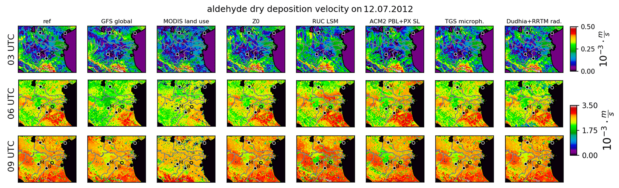
Figure 4Dry deposition velocities of aldehyde on 12 July 2012 at 03:00, 06:00 and 09:00 UTC (coded by color) for different model configurations, including increased roughness length (“Z0”). Plotting conventions are like in Fig. 2.
Using RUC LSM results in larger dry deposition velocities in the central Po Valley at all times. Boundary layer and surface layer schemes induce local effects with opposite signs after sunrise south of Modena and east of Verona, respectively. The selection of the microphysics schemes induces only minor local changes in this case (Fig. 4; “microph.”). The largest effect of Dudhia short-wave and RRTM long-wave radiation schemes appears at 06:00 UTC when dry deposition velocities are decreased in the northern part of the domain (Fig. 4; “rad.”).
4.3 Effects on pollutant transport
This section investigates effects on the transport of any atmospheric pollutant. Section 4.3.1 evaluates effects on fields of friction velocity forecasted by WRF-ARW. As friction velocities only provide information on the horizontal wind speeds determining pollutant advection, source regions of air masses indicate total effects of atmospheric dynamics. An analysis of source regions of a representative air mass is given in Sect. 4.3.2.
4.3.1 Effects on friction velocities
In general, friction velocities do not change substantially between nighttime and daytime but increase in most areas with increasing local instability. For the reference setup in Fig. 5, high values predicted at 03:00 UTC over the peaks of the Apennines are almost 1 order of magnitude higher than in the rest of the domain. After sunrise, these large differences reduce over time by increasing mean values and slightly decreasing peak values. GFS global meteorology indicates reduced friction velocities in the central Po Valley, especially at 06:00 UTC (Fig. 5; “global”). Effects of land use information appear to influence friction velocities on comparably small scales (Fig. 5; “land use”). Using MODIS instead of USGS, friction velocities are partly increased in the northeastern part of the domain. Friction velocities appear also to be only a little sensitive to increased roughness length, inducing slightly increased values after sunrise (Fig. 5; “Z0”).

Figure 5Friction velocities on 12 July 2012 at 03:00, 06:00 and 09:00 UTC (coded by color) for different model configurations, including increased roughness length (“Z0”). Plotting conventions are like in Fig. 2.
The selection of the LSM, boundary layer and surface layer schemes induces significant effects on friction velocities (Fig. 5; “LSM” plus “PBL+SL”). As early as 03:00 UTC, the RUC LSM triggers a region of increased values south of Lake Garda. This signal penetrates along the Po River affecting large parts of the valley from 06:00 to 09:00 UTC, resulting in almost doubled friction velocities. Similar to the sensitivity to the LSM, friction velocities are partly increased in the central Po Valley by the ACM2 boundary layer and Pleim–Xiu surface layer schemes. However, this effect is less pronounced, and regions of high values change with time. At the northeastern edge north of Venice, friction velocities are increased for all times. Microphysics and radiation parameterizations only induce minor changes in friction velocities (Fig. 5; “microph.”, “rad.”). Slightly changed patterns due to Dudhia short-wave and RRTM long-wave radiation schemes are observed in the western and eastern Po Valley at 06:00 and 09:00 UTC, respectively.
4.3.2 Effects on source regions
Although differences in friction velocities do not vary substantially in this case, an investigation of the air masses' history provides more detailed information on pollutant transport. The analysis of the meteorological conditions states the overall reproducibility of the observed local conditions by all simulations used in this study (Sect. 2.1). At the same time, the simulations show low-level variable wind directions related to the low wind speeds which might result in diverging pollutant transport. Some studies are available that investigate the history of air masses in the Po Valley by means of long-term backward trajectories (Sogacheva et al., 2007; Pernigotti et al., 2012; Sullivan et al., 2016). However, this approach does not account for local effects and related uncertainties in transport and mixing. Here, these effects are analyzed using retroplume calculations for a representative air parcel. The selected air mass is located at the position of the zeppelin's observations (44.7∘ N, 11.6∘ E; “target location”) on 12 July 2012 at 06:00 UTC (“target time”) at 100 m height above sea level. Starting at this time, the retroplume calculation provides relative contributions of source areas of this air mass backward in time. The zeppelin's observations were performed close to the base station of the zeppelin at San Pietro Capofiume (SPC) in the southeastern part of the Po Valley. Being located approximately 30 km northeast of Bologna, SPC is classified as a urban background site (Kaiser et al., 2015; Rosati et al., 2016b). However, Sandrini et al. (2016) state that it might be affected by Bologna's urban area in the case of southwesterly winds.
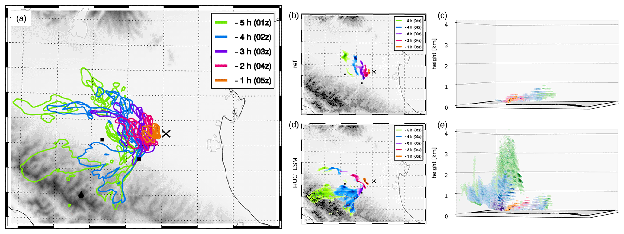
Figure 6Horizontal (a, b, d) and vertical (c, e) distributions of source regions for 44.7∘ N, 11.6∘ E and 100 m a.s.l. (black cross is target location) on 12 July 2012 at 06:00 UTC. (a) Significant contributions to vertically integrated source regions for all model configurations, including increased roughness length, are given as isolines (colored by time according to legend). Gray colors indicate the surface topography. Panels (b) and (c) reference the configuration and (d) and (e) RUC LSM. For (b) and (d), the viewing direction is from east-northeast towards west-southwest.
Figure 6b and c show the evolution of source regions for the reference setup. The selected air mass is advected from western to northwestern directions due to slow westerly winds. During the last 3 h before the target time, the air mass converged horizontally by meridional mixing processes. Thus, contributions of this air mass converge from southwestern to northwestern directions at this time. The major source of the air mass 5 h before is found northwest of the target location. During the entire time interval, the vertical extension of source areas remains below 1 km altitude (Fig. 6c). This is caused by low vertical mixing, which is typical for the early morning hours over flat terrain.
By applying different kinds of model configurations, the resulting effects on horizontal source regions are shown in Fig. 6a. Horizontal source areas start to diverge already during the first hours before the target time. Significant contributions 3 h earlier span from Bologna in the southwest for RUC LSM to the western central Po Valley in the northwest for GFS global meteorology. Additional differences in transport distance and vertical mixing become visible 5 h before. Transport distances from the selected target location vary by more than a factor of 2 at this time. For example, source regions for the ACM2 boundary layer and Pleim–Xiu surface layer schemes almost extend to the western boundary of the domain within 5 h. This is caused by increased turbulent transport compared to the reference MYJ boundary layer and Eta surface layer schemes. In contrast, the Dudhia and RRTM radiation schemes, as well as MODIS land use information, indicate slow horizontal transport from urban areas close to Modena and Bologna. Compared to mainly agricultural source areas for the reference and ACM2, these slight changes in local dynamics may result in significant changes in the composition of this air mass.
As shown in Fig. 6d and e, the RUC LSM has the greatest effect on the simulated air mass history. In the horizontal plane, a major contribution to the air mass was transported from southwestern directions crossing Bologna. Prior to this, it descended from the Apennine Mountains where high wind speeds advect air from comparably remote source regions. This is related to increased mixing processes which result in large extended source regions 4 h before. Between 4 and 5 h before, the source areas show the convergence of two distinct air masses flowing around the highest peaks of Monte Cimone with altitudes of more than 2000 m a.s.l. (Fig. 6d). The overflow above the Apennines forces the air mass to source altitudes of up to 4 km a.s.l. 5 h before the target time. Additionally, a small contribution of the air mass originates from a narrow valley southwest of Bologna with lower wind speeds and source altitudes of below 1 km a.s.l. (lower left part of Fig. 6e).
Simulations of near-surface concentrations of trace gases are controlled by the model processes as discussed above. The evaluation of biogenic gas concentrations is restricted to isoprene because of its direct dependency on the model processes discussed above. Other biogenic gases are affected by additional processes like secondary production which hamper a detailed evaluation. Instead, resulting OH concentrations are analyzed for their impact on reactive atmospheric chemistry. As microphysics and radiation schemes appear to have only minor effects on the model processes in this case, their effects on concentrations are not further discussed.
5.1 Effects on isoprene
Being a short-lived biogenic trace gas, isoprene concentrations are mainly determined by changes in biogenic emissions, as shown in Fig. 7. Consequently, effects of land use information and drought response on isoprene emissions transfer almost directly to differences in surface concentrations. Using MODIS land use produces negligible isoprene concentrations within the Po Valley and increased concentrations in the mountains. An overall increase in isoprene concentrations is achieved at all times when no emission response to soil dryness is considered.
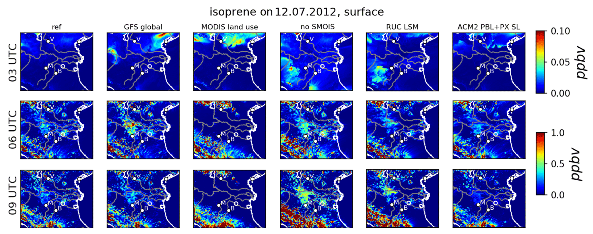
Figure 7Isoprene surface concentrations on 12 July 2012 at 03:00, 06:00 and 09:00 UTC (coded by color) for different model configurations. Plotting conventions are like in Fig. 2.
Nevertheless, effects of atmospheric transport do also influence isoprene concentrations when changing modeled global meteorology, as well as LSM and boundary layer schemes. At 06:00 UTC, surface concentrations north of Modena are increased for GFS global meteorology, although local emissions were slightly reduced (compare with Sect. 4.1). This is caused by higher atmospheric stability leading to less dispersion, which is indicated by reduced friction velocities (compare with Sect. 4.3.1). For the RUC LSM, increased isoprene emissions are partly compensated for by increased mixing in the central valley after sunrise. Thus, the most significant increase in surface concentrations is found in the Apennine Mountains. Effects of combined boundary layer and surface layer schemes do appear on local scales due to slightly reduced emissions and variable dynamical effects.
5.2 Effects on OH
The hydroxy radical OH is a highly reactive oxidant in the atmosphere acting as the most important sink of isoprene (Kaser et al., 2015). Generally, OH may be influenced by the model configuration via reactions with biogenically emitted gases and meteorological conditions. Local meteorology mainly affects OH by changes in radiation related to humidity and clouds. In this specific case, the weather in the Po region was continuously characterized by clear and dry conditions as described in Sect. 2.1. Thus, no significant differences in humidity and cloud coverage are simulated by the model configurations (not shown). This makes the differences in OH concentrations determined by changed BVOCs.

Figure 8OH surface concentrations on 12 July 2012 at 06:00 and 09:00 UTC (coded by color) for different model configurations. Plotting conventions are like in Fig. 2.
As expected from atmospheric chemistry, daytime OH concentrations shown in Fig. 8 are reduced in regions of high BVOC concentrations like the central Po Valley and the southern Apennines. In contrast, OH concentrations remain comparably high in the mountains and over the ocean where isoprene concentrations are neglectable. This direct dependence of OH to biogenic gases causes also significant differences in OH concentrations with respect to model configuration. In this case, the effects are most dominant in cases of increased isoprene concentrations with respect to the reference simulation. A significant reduction in OH is induced by excluding drought response (no SMOIS), RUC LSM and, although less pronounced, MODIS land use in the southern Apennines. While these reductions are persistent in time, increased isoprene concentrations in the central Po Valley for GFS global meteorology at 06:00 UTC result in temporally reduced OH concentrations in this region.
The case analysis in Sect. 4.1 indicates almost constant effects of model configurations, especially for biogenic emissions. Thus, the results can be comprised of temporally averaged sensitivities to biogenic emissions for a set of representative cases during the campaign. Sensitivity factors are calculated as the temporal average of emissions at each time divided by their corresponding values from the reference configuration. While for 1 and 12 July 2012 the analysis focuses on the morning hours between 00:00 and 10:00 UTC, evening conditions between 12:00 and 22:00 UTC are investigated for the 7 July 2012 case. Note that minimum emissions of are defined in order to avoid unrealistically large factors induced by low values.
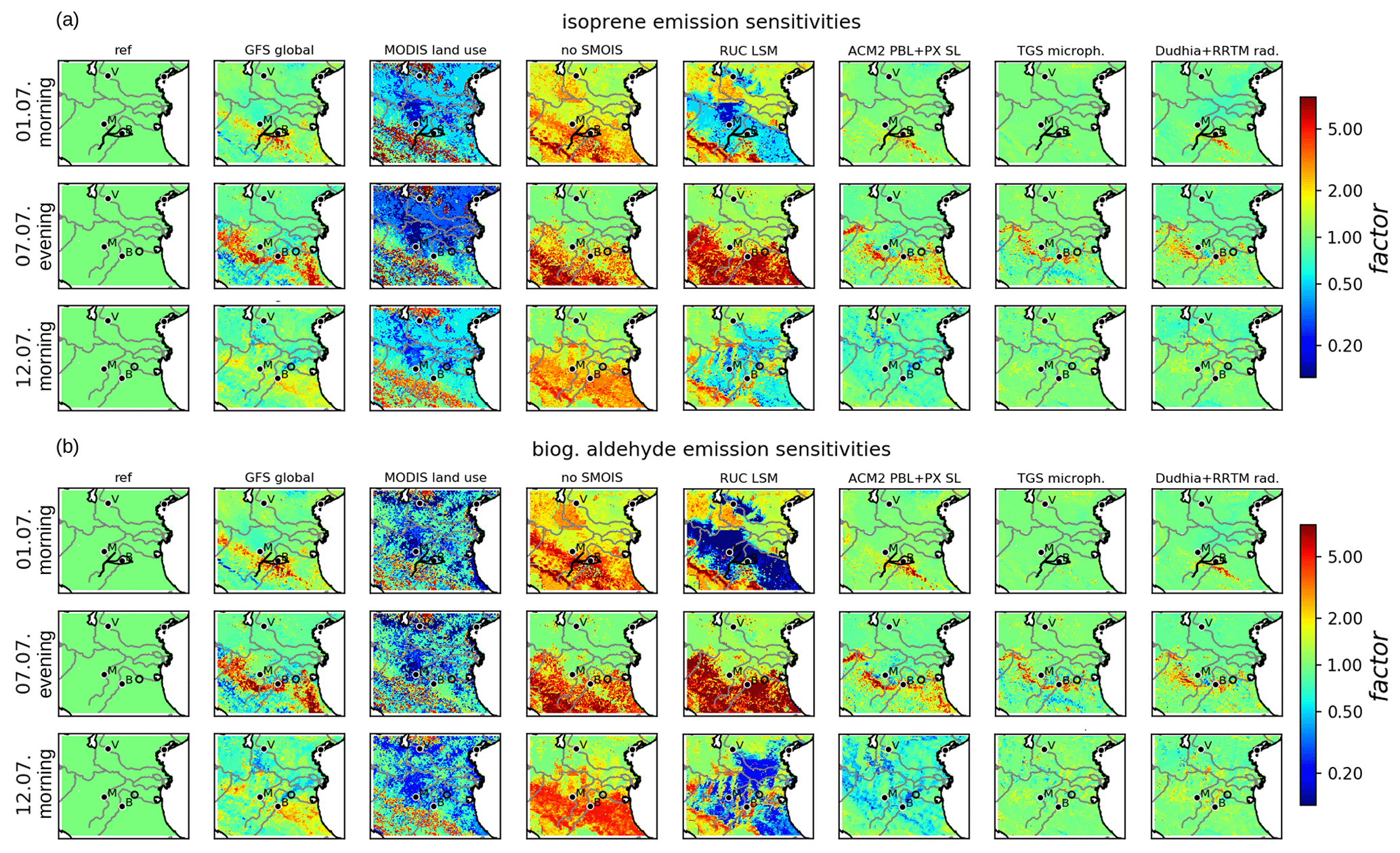
Figure 9Averaged sensitivities to isoprene (a) and biogenic aldehyde (b) emissions on 1 July morning (00:00–10:00 UTC), 7 July evening (12:00–22:00 UTC) and 12 July morning (00:00–10:00 UTC) (temporally averaged factors with respect to reference; coded by color) for different model configurations. Plotting conventions are like in Fig. 2.
As shown in Fig. 9, sensitivities to both biogenic gases during the campaign are most significant for land use, drought response and the LSM. As expected, the large averaged sensitivities to land use information are highly similar for all cases and both gases. Somewhat lower averaged sensitivities to isoprene on 1 and 12 July are induced by emissions below the minimum value in the early morning. A strong increase in emissions due to neglected drought response is found for all cases with the most significant effects in the southern part of the domain.
For the two morning cases (1 and 12 July) RUC LSM results in reduced emissions in most parts of the Po Valley and increased values south of Verona and in the southwest. In contrast, highly increased biogenic emissions are produced in the entire southern half of the domain during the evening case (7 July). These diurnal differences are caused by generally different temporal evolutions of soil moisture which limit biogenic emissions. While soil moisture from Pleim–Xiu LSM drops during daytime and recovers quickly during nighttime, RUC predicts a continuous decrease during these days. Thus, lower soil moisture for RUC induces lower emissions in the morning, and vise versa in the evening. Despite these general diurnal differences, sensitivities in the LSM appear to be mostly constant during the campaign.
The use of GFS global meteorology induces small yet similar effects for all cases. While emissions are elevated in the northern Apennines, emissions tend to be slightly lower elsewhere. Effects of boundary layer and surface layer schemes remain small and differ between the cases. While for 12 July the ACM2 boundary layer and Pleim–Xiu surface layer schemes induce decreased biogenic emissions, they produce increased emissions north of the Apennines in the other cases. Microphysics and radiation schemes induce only significant effects in the evening case (7 July) with slightly increased emissions north of the Apennines.
Forecasts of biogenic trace gases in the PBL are well known to be subject to large uncertainties. The PEGASOS campaign in the Po Valley in 2012 provides a challenging, yet common, environment for investigating model uncertainties with a focus on biogenic gases in the PBL. As a precursory step to probabilistic model evaluation with PEGASOS observations, this study identifies and quantifies principal sources of forecast uncertainties induced by model configurations via different model processes. Two major pathways of model uncertainties with respect to model parameters and inputs are identified in this study.
Firstly, exceptionally large differences in simulated biogenic emissions are found in the Po Valley during the campaign. Dominating the impacts of land use information, the land surface model and emission response to drought state a high sensitivity of biogenic emissions to various land surface conditions. Although biogenic emissions are known to be affected by environmental conditions, these three effects induce unexpectedly high variations of up to an order of magnitude in the studied case. Due to the common approach used for modeling biogenic emissions, the results appear to be highly correlated for different biogenic gases. Moreover, these effects are found to be almost constant during the campaign, varying only with the diurnal cycle. Despite invariant vegetation distributions, this persistence is forced by steady meteorological conditions during the campaign.
Secondly, the model configuration also highly influences regional flow patterns with effects on pollutant transport and mixing. Especially the selection of land surface model and boundary layer schemes induces significant differences in local pollutant transport. Although effects on friction velocities remain small, diverging source regions prove high sensitivities of pollutant transport to the selected model configurations, which applies also to non-biogenic gases. The most prominent changes in horizontal advection and vertical mixing patterns induced by the land surface model can be attributed to differences in surface heat exchange. In this study, the selection of cloud microphysics and radiation schemes only induces minor uncertainties during this study. This is due to the calm and sunny conditions in the Po Valley and may be more significant for other meteorological conditions.
As a result, surface concentrations of isoprene show large sensitivities to model configurations. These sensitivities are mainly induced by changes in land use information, the land surface model and drought response via their impact on emissions. Moreover, changes in surface concentrations of biogenic trace gases induce significant differences in OH concentrations affecting reactive atmospheric chemistry. Excluding the emission response to drought stress reduces local OH concentrations by up to a factor of 3 in this study. Despite these dominant effects of biogenic emissions, highly variable transport patterns with respect to the land surface model and boundary layer schemes are likely to affect local composition significantly. Thus, especially in such areas with small-scale emission patterns, the selection of the model configuration may result in highly variable local concentrations.
Although the presented results are specific for the conditions in the Po Valley, it can be claimed that forecasts of biogenic gases would generally benefit substantially from improved representation of the land surface. While improved land use information could be retrieved from more recent satellite products like Sentinel-2, considerably different effects of land surface models for both biogenic emissions and pollutant transport underline the significance of soil moisture estimates for air-quality modeling. Furthermore, the large amount and complexity of sensitivities found in this study demonstrate the need to account for forecast uncertainties with special focus on biogenic emissions and pollutant transport. This is especially important for model evaluation with observations, as well as chemical data assimilation in the PBL. A follow-up study will evaluate probabilistic model forecasts of biogenic gases using airborne PEGASOS observations of biogenic gases. In this context, the sensitivities derived in this study provide a basis for estimating forecast uncertainties with respect to different model processes.
The model data produced for this study are stored locally at the Rhenish Institute for Environmental Research and at the Jülich Supercomputer Centre (JSC) of Research Centre Jülich. They are available on request via email (av@eurad.uni-koeln.de).
AV performed the simulations, analyzed the results and wrote the paper. HE supervised the work, contributed significantly to the analysis and helped in the preparation of the paper.
The authors declare that they have no conflict of interest.
The author gratefully acknowledges the computing time granted through JARA-HPC on the supercomputer JURECA (Jülich Supercomputing Centre, 2018) at Forschungszentrum Jülich. This work would not have been possible without the meteorological analysis obtained from the NCEP's Global Forecasting System (GFS). The authors thank two anonymous reviewers for their valuable suggestions.
This research has been supported by the Helmholtz Climate Initiative REKLIM (Regional Climate Change) (grant no. REKLIM-2009-07-16).
The article processing charges for this open-access
publication were covered by a Research
Centre of the Helmholtz Association.
This paper was edited by Manish Shrivastava and reviewed by two anonymous referees.
Anderson, R., Hardy, E. E., Roach, J. T., and Witmer, R. E.: A land use and land cover classification system for use with remote sensor data, Report, USGS Prof. Pap, 964, https://doi.org/10.3133/pp964, 1976. a
Arakawa, A. and Lamb, V.: Computational design of the basic dynamical processes of the UCLA general circulation model, Meth. Comput. Phys., 17, 173–265, 1977. a
Arneth, A., Monson, R. K., Schurgers, G., Niinemets, Ü., and Palmer, P. I.: Why are estimates of global terrestrial isoprene emissions so similar (and why is this not so for monoterpenes)?, Atmos. Chem. Phys., 8, 4605–4620, https://doi.org/10.5194/acp-8-4605-2008, 2008. a
Arneth, A., Schurgers, G., Lathiere, J., Duhl, T., Beerling, D. J., Hewitt, C. N., Martin, M., and Guenther, A.: Global terrestrial isoprene emission models: sensitivity to variability in climate and vegetation, Atmos. Chem. Phys., 11, 8037–8052, https://doi.org/10.5194/acp-11-8037-2011, 2011. a
Banks, R. F., Tiana-Alsina, J., Baldasano, J. M., Rocadenbosch, F., Papayannis, A., Solomos, S., and Tzanis, C. G.: Sensitivity of boundary-layer variables to PBL schemes in the WRF model based on surface meteorological observations, lidar, and radiosondes during the HygrA-CD campaign, Atmos. Res., 176, 185–201, https://doi.org/10.1016/j.atmosres.2016.02.024, 2016. a
Benjamin, S. G., Grell, G. A., Brown, J. M., Smirnova, T. G., and Bleck, R.: Mesoscale Weather Prediction with the RUC Hybrid Isentropic–Terrain-Following Coordinate Model, Mon. Weather Rev., 132, 473–494, https://doi.org/10.1175/1520-0493(2004)132<0473:MWPWTR>2.0.CO;2, 2004. a
Berndt, J.: On the predictability of exceptional error events in wind power forecasting – an ultra large ensemble approach, PhD thesis, University of Cologne, Germany, 2018. a, b, c
Bucci, S., Cristofanelli, P., Decesari, S., Marinoni, A., Sandrini, S., Größ, J., Wiedensohler, A., Di Marco, C. F., Nemitz, E., Cairo, F., Di Liberto, L., and Fierli, F.: Vertical distribution of aerosol optical properties in the Po Valley during the 2012 summer campaigns, Atmos. Chem. Phys., 18, 5371–5389, https://doi.org/10.5194/acp-18-5371-2018, 2018. a
Caplan, P., Derber, J., Gemmill, W., Hong, S.-Y., Pan, H.-L., and Parrish, D.: Changes to the 1995 NCEP Operational Medium-Range Forecast Model Analysis Forecast System, Weather Forecast. 12, 581–594, https://doi.org/10.1175/1520-0434(1997)012<0581:CTTNOM>2.0.CO;2, 1997. a
Chen, B., Yang, S., Xu, X.-D., and Zhang, W.: The impacts of urbanization on air quality over the Pearl River Delta in winter: roles of urban land use and emission distribution, Theor. Appl. Climatol., 117, 29–39, https://doi.org/10.1007/s00704-013-0982-1, 2014. a
Chen, T., Chu, B., Ge, Y., Zhang, S., Ma, Q., He, H., and Li, S.-M.: Enhancement of aqueous sulfate formation by the coexistence of NO2/NH3 under high ionic strengths in aerosol water, Environ. Pollut., 252, 236–244, https://doi.org/10.1016/j.envpol.2019.05.119, 2019. a
Dee, D. P., Uppala, S. M., Simmons, A. J., Berrisford, P., Poli, P., Kobayashi, S., Andrae, U., Balmaseda, M. A., Balsamo, G., Bauer, P., Bechtold, P., Beljaars, A. C. M., van de Berg, L., Bidlot, J., Bormann, N., Delsol, C., Dragani, R., Fuentes, M., Geer, A. J., Haimberger, L., Healy, S. B., Hersbach, H., Hólm, E. V., Isaksen, L., Kållberg, P., Köhler, M., Matricardi, M., McNally, A. P., Monge-Sanz, B. M., Morcrette, J.-J., Park, B.-K., Peubey, C., de Rosnay, P., Tavolato, C., Thépaut, J.-N., and Vitart, F.: The ERA-Interim reanalysis: configuration and performance of the data assimilation system, Q. J. Roy. Meteor. Soc., 137, 553–597, https://doi.org/10.1002/qj.828, 2011. a
Drusch, M., Bello, U. D., Carlier, S., Colin, O., Fernandez, V., Gascon, F., Hoersch, B., Isola, C., Laberinti, P., Martimort, P., Meygret, A., Spoto, F., Sy, O., Marchese, F., and Bargellini, P.: Sentinel-2: ESA's Optical High-Resolution Mission for GMES Operational Services, Remote Sens. Environ., 120, 25–36, https://doi.org/10.1016/j.rse.2011.11.026, 2012. a
Dudhia, J.: Numerical Study of Convection Observed during the Winter Monsoon Experiment Using a Mesoscale Two-Dimensional Model, J. Atmos. Sci., 46, 3077–3107, https://doi.org/10.1175/1520-0469(1989)046<3077:NSOCOD>2.0.CO;2, 1989. a
Eder, B., Kang, D., Mathur, R., Yu, S., and Schere, K.: An operational evaluation of the Eta–CMAQ air quality forecast model, Atmos. Environ., 40, 4894–4905, https://doi.org/10.1016/j.atmosenv.2005.12.062, 2006. a
Elbern, H., Strunk, A., Schmidt, H., and Talagrand, O.: Emission rate and chemical state estimation by 4-dimensional variational inversion, Atmos. Chem. Phys., 7, 3749–3769, https://doi.org/10.5194/acp-7-3749-2007, 2007. a, b
Emili, E., Gürol, S., and Cariolle, D.: Accounting for model error in air quality forecasts: an application of 4DEnVar to the assimilation of atmospheric composition using QG-Chem 1.0, Geosci. Model Dev., 9, 3933–3959, https://doi.org/10.5194/gmd-9-3933-2016, 2016. a
Finardi, S., Silibello, C., D'Allura, A., and Radice, P.: Analysis of pollutants exchange between the Po Valley and the surrounding European region, Urban Climate, 10, 682–702, https://doi.org/10.1016/j.uclim.2014.02.002, 2014. a, b
Friedl, M., McIver, D., Hodges, J., Zhang, X., Muchoney, D., Strahler, A., Woodcock, C., Gopal, S., Schneider, A., Cooper, A., Baccini, A., Gao, F., and Schaaf, C.: Global land cover mapping from MODIS: algorithms and early results, Remote Sens. Environ., 83, 287–302, https://doi.org/10.1016/S0034-4257(02)00078-0, 2002. a
Gama, C., Ribeiro, I., Lange, A., Vogel, A., Ascenso, A., Seixas, V., Elbern, H., Borrego, C., Friese, E., and Monteiro, A.: Performance assessment of CHIMERE and EURAD-IM’ dust modules, Atmos. Pollut. Res., 10, 1336–1346, https://doi.org/10.1016/j.apr.2019.03.005, 2019. a
Geiger, H., Barnes, I., Bejan, I., Benter, T., and Spittler, M.: The tropospheric degradation of isoprene: An updated module for the regional atmospheric chemistry mechanism, Atmos. Environ., 37, 1503–1519, https://doi.org/10.1016/S1352-2310(02)01047-6, 2003. a
Geng, F., Tie, X., Guenther, A., Li, G., Cao, J., and Harley, P.: Effect of isoprene emissions from major forests on ozone formation in the city of Shanghai, China, Atmos. Chem. Phys., 11, 10449–10459, https://doi.org/10.5194/acp-11-10449-2011, 2011. a, b
Guenther, A. B., Jiang, X., Heald, C. L., Sakulyanontvittaya, T., Duhl, T., Emmons, L. K., and Wang, X.: The Model of Emissions of Gases and Aerosols from Nature version 2.1 (MEGAN2.1): an extended and updated framework for modeling biogenic emissions, Geosci. Model Dev., 5, 1471–1492, https://doi.org/10.5194/gmd-5-1471-2012, 2012. a, b, c, d, e
Hansen, M. C., DeFries, R. S., Townshend, J. R. G., Sohlberg, R., Dimiceli, C., and Carroll, M.: Towards an operational MODIS continuous field of percent tree cover algorithm: examples using AVHRR and MODIS data, Remote Sens. Environ., 83, 303–319, https://doi.org/10.1016/S0034-4257(02)00079-2, 2002. a
Hass, H., Jakobs, H. J., and Memmesheimer, M.: Analysis of a regional model (EURAD) near surface gas concentration predictions using observations from networks, Meteorol. Atmos. Phys., 57, 173–200, https://doi.org/10.1007/BF01044160, 1995. a
Henrot, A.-J., Stanelle, T., Schröder, S., Siegenthaler, C., Taraborrelli, D., and Schultz, M. G.: Implementation of the MEGAN (v2.1) biogenic emission model in the ECHAM6-HAMMOZ chemistry climate model, Geosci. Model Dev., 10, 903–926, https://doi.org/10.5194/gmd-10-903-2017, 2017. a
Hong, S. and Lim, J. J.: The WRF Single-Moment 6-Class Microphysics Scheme (WSM6), J. Korean Meteor. Soc., 42, 129–151, 2006. a
Hortal, M.: Formulation of the ECMWF Forecast Model, Springer Netherlands, Dordrecht, 237–251, https://doi.org/10.1007/978-94-015-9137-9_10,1998. a
Hu, X., Nielsen-Gammon, J., and Zhang, F.: Evaluation of three planetary boundary layer schemes in the WRF model, J. Appl. Meteorol. Clim., 49, 1831–1844, https://doi.org/10.1175/2010JAMC2432.1, 2010. a
Iacono, M. J., Delamere, J. S., Mlawer, E. J., Shephard, M. W., Clough, S. A., and Collins, W. D.: Radiative forcing by long-lived greenhouse gases: Calculations with the AER radiative transfer models, J. Geophys. Res.-Atmos., 113, D13103, https://doi.org/10.1029/2008JD009944, 2008. a
Immitzer, M., Vuolo, F., and Atzberger, C.: First Experience with Sentinel-2 Data for Crop and Tree Species Classifications in Central Europe, Remote Sens., 8, 166, https://doi.org/10.3390/rs8030166, 2016. a
Israelevich, P., Ganor, E., Alpert, P., Kishcha, P., and Stupp, A.: Predominant transport paths of Saharan dust over the Mediterranean Sea to Europe, J. Geophys. Res.-Atmos., 117, D02205, https://doi.org/10.1029/2011JD016482, 2012. a
Jäger, J.: Airborne VOC Measurements on board the Zeppelin NT during the PEGASOS campaigns in 2012 deploying the improved Fast-GC-MSD System, PhD thesis, University of Cologne, Germany, 2013. a, b
Janjic, Z. I.: The Step-Mountain Eta Coordinate Model: Further Developments of the Convection, Viscous Sublayer, and Turbulence Closure Schemes, Mon. Weather Rev., 122, 927–945, https://doi.org/10.1175/1520-0493(1994)122<0927:TSMECM>2.0.CO;2, 1994. a
Janjic, Z. I.: The Mellor-Yamada level 2.5 scheme in the NCEP Eta Model, 11th Conference on Numerical Weather Prediction, American Meteorological Society, 19–23 August 1996, Norfolk, VA, 333–334, 1996. a
Jiang, X., Guenther, A., Potosnak, M., Geron, C., Seco, R., Karl, T., Kim, S., Gu, L., and Pallardy, S.: Isoprene emission response to drought and the impact on global atmospheric chemistry, Atmos. Environ., 183, 69–83, https://doi.org/10.1016/j.atmosenv.2018.01.026, 2018. a
Jülich Supercomputing Centre: JURECA: Modular supercomputer at Jülich Supercomputing Centre, J. Large-Scale Res. Facilities, 4, A132, https://doi.org/10.17815/jlsrf-4-121-1, 2018. a
Kaiser, J., Wolfe, G. M., Bohn, B., Broch, S., Fuchs, H., Ganzeveld, L. N., Gomm, S., Häseler, R., Hofzumahaus, A., Holland, F., Jäger, J., Li, X., Lohse, I., Lu, K., Prévôt, A. S. H., Rohrer, F., Wegener, R., Wolf, R., Mentel, T. F., Kiendler-Scharr, A., Wahner, A., and Keutsch, F. N.: Evidence for an unidentified non-photochemical ground-level source of formaldehyde in the Po Valley with potential implications for ozone production, Atmos. Chem. Phys., 15, 1289–1298, https://doi.org/10.5194/acp-15-1289-2015, 2015. a, b, c
Karnezi, E., Murphy, B. N., Poulain, L., Herrmann, H., Wiedensohler, A., Rubach, F., Kiendler-Scharr, A., Mentel, T. F., and Pandis, S. N.: Simulation of atmospheric organic aerosol using its volatility–oxygen-content distribution during the PEGASOS 2012 campaign, Atmos. Chem. Phys., 18, 10759–10772, https://doi.org/10.5194/acp-18-10759-2018, 2018. a, b
Kaser, L., Karl, T., Yuan, B., Mauldin III, R. L., Cantrell, C. A., Guenther, A. B., Patton, E. G., Weinheimer, A. J., Knote, C., Orlando, J., Emmons, L., Apel, E., Hornbrook, R., Shertz, S., Ullmann, K., Hall, S., Graus, M., de Gouw, J., Zhou, X., and Ye, C.: Chemistry-turbulence interactions and mesoscale variability influence the cleansing efficiency of the atmosphere, Geophys. Res. Lett., 42, 10894–10903, https://doi.org/10.1002/2015GL066641, 2015. a, b
Kontkanen, J., Järvinen, E., Manninen, H. E., Lehtipalo, K., Kangasluoma, J., Decesari, S., Gobbi, G. P., Laaksonen, A., Petäjä, T., and Kulmala, M.: High concentrations of sub-3 nm clusters and frequent new particle formation observed in the Po Valley, Italy, during the PEGASOS 2012 campaign, Atmos. Chem. Phys., 16, 1919–1935, https://doi.org/10.5194/acp-16-1919-2016, 2016. a, b, c, d
Krinner, G., Viovy, N., de Noblet-Ducoudre, N., Ogee, J., Polcher, J., Friedlingstein, P., Ciais, P., Sitch, S., and Prentice, I.: A dynamic global vegetation model for studies of the coupled atmosphere-biosphere system, Global Biogeochem. Cy., 19, GB1015, https://doi.org/10.1029/2003GB002199, 2005. a
Kuenen, J. J. P., Visschedijk, A. J. H., Jozwicka, M., and Denier van der Gon, H. A. C.: TNO-MACC_II emission inventory; a multi-year (2003–2009) consistent high-resolution European emission inventory for air quality modelling, Atmos. Chem. Phys., 14, 10963–10976, https://doi.org/10.5194/acp-14-10963-2014, 2014. a
Lavoir, A.-V., Staudt, M., Schnitzler, J. P., Landais, D., Massol, F., Rocheteau, A., Rodriguez, R., Zimmer, I., and Rambal, S.: Drought reduced monoterpene emissions from the evergreen Mediterranean oak Quercus ilex: results from a throughfall displacement experiment, Biogeosciences, 6, 1167–1180, https://doi.org/10.5194/bg-6-1167-2009, 2009. a
Li, X., Rohrer, F., Hofzumahaus, A., Brauers, T., Häseler, R., Bohn, B., Broch, S., Fuchs, H., Gomm, S., Holland, F., Jäger, J., Kaiser, J., Keutsch, F. N., Lohse, I., Lu, K., Tillmann, R., Wegener, R., Wolfe, G. M., Mentel, T. F., Kiendler-Scharr, A., and Wahner, A.: Missing Gas-Phase Source of HONO Inferred from Zeppelin Measurements in the Troposphere, Science, 344, 292–296, https://doi.org/10.1126/science.1248999, 2014. a, b
Loveland, T. R., Reed, B. C., Brown, J. F., Ohlen, D. O., Zhu, Z., Yang, L., and Merchant, J. W.: Development of a global land cover characteristics database and IGBP DISCover from 1 km AVHRR data, Int. J. Remote Sens., 21, 1303–1330, https://doi.org/10.1080/014311600210191, 2000. a
Ma, J. and van Aardenne, J. A.: Impact of different emission inventories on simulated tropospheric ozone over China: a regional chemical transport model evaluation, Atmos. Chem. Phys., 4, 877–887, https://doi.org/10.5194/acp-4-877-2004, 2004. a
Mentel, Th. F., Kleist, E., Andres, S., Dal Maso, M., Hohaus, T., Kiendler-Scharr, A., Rudich, Y., Springer, M., Tillmann, R., Uerlings, R., Wahner, A., and Wildt, J.: Secondary aerosol formation from stress-induced biogenic emissions and possible climate feedbacks, Atmos. Chem. Phys., 13, 8755–8770, https://doi.org/10.5194/acp-13-8755-2013, 2013. a
Mlawer, E. J., Taubman, S. J., Brown, P. D., Iacono, M. J., and Clough, S. A.: Radiative transfer for inhomogeneous atmospheres: RRTM, a validated correlated-k model for the longwave, J. Geophys. Res.-Atmos., 102, 16663–16682, https://doi.org/10.1029/97JD00237, 1997. a
Pegoraro, E., Rey, A., Greenberg, J., Harley, P., Grace, J., Malhi, Y., and Guenther, A.: Effect of drought on isoprene emission rates from leaves of Quercus virginiana Mill., Atmos. Environ., 38, 6149–6156, https://doi.org/10.1016/j.atmosenv.2004.07.028, 2004. a
Pernigotti, D., Georgieva, E., Thunis, P., and Bessagnet, B.: Impact of meteorology on air quality modeling over the Po valley in northern Italy, Atmos. Environ., 51, 303–310, https://doi.org/10.1016/j.atmosenv.2011.12.059, 2012. a
Pleim, J. E.: A Simple, Efficient Solution of Flux–Profile Relationships in the Atmospheric Surface Layer, J. Appl. Meteorol. Clim., 45, 341–347, https://doi.org/10.1175/JAM2339.1, 2006. a
Pleim, J. E.: A Combined Local and Nonlocal Closure Model for the Atmospheric Boundary Layer. Part II: Application and Evaluation in a Mesoscale Meteorological Model, J. Appl. Meteorol. Clim., 46, 1396–1409, https://doi.org/10.1175/JAM2534.1, 2007. a
Pleim, J. E. and Xiu, A.: Development and Testing of a Surface Flux and Planetary Boundary Layer Model for Application in Mesoscale Models, J. Appl. Meteorol., 34, 16–32, https://doi.org/10.1175/1520-0450-34.1.16, 1995. a
Pöschl, U., Kuhlmann, R., Poisson, N., and Crutzen, P.: Development and Intercomparison of Condensed Isoprene Oxidation Mechanisms for Global Atmospheric Modeling, J. Atmos. Chem., 37, 29–52, https://doi.org/10.1023/A:1006391009798, 2000. a
Rinaldi, M., Gilardoni, S., Paglione, M., Sandrini, S., Fuzzi, S., Massoli, P., Bonasoni, P., Cristofanelli, P., Marinoni, A., Poluzzi, V., and Decesari, S.: Organic aerosol evolution and transport observed at Mt. Cimone (2165 m a.s.l.), Italy, during the PEGASOS campaign, Atmos. Chem. Phys., 15, 11327–11340, https://doi.org/10.5194/acp-15-11327-2015, 2015. a
Rosati, B., Gysel, M., Rubach, F., Mentel, T. F., Goger, B., Poulain, L., Schlag, P., Miettinen, P., Pajunoja, A., Virtanen, A., Klein Baltink, H., Henzing, J. S. B., Größ, J., Gobbi, G. P., Wiedensohler, A., Kiendler-Scharr, A., Decesari, S., Facchini, M. C., Weingartner, E., and Baltensperger, U.: Vertical profiling of aerosol hygroscopic properties in the planetary boundary layer during the PEGASOS campaigns, Atmos. Chem. Phys., 16, 7295–7315, https://doi.org/10.5194/acp-16-7295-2016, 2016a. a
Rosati, B., Herrmann, E., Bucci, S., Fierli, F., Cairo, F., Gysel, M., Tillmann, R., Größ, J., Gobbi, G. P., Di Liberto, L., Di Donfrancesco, G., Wiedensohler, A., Weingartner, E., Virtanen, A., Mentel, T. F., and Baltensperger, U.: Studying the vertical aerosol extinction coefficient by comparing in situ airborne data and elastic backscatter lidar, Atmos. Chem. Phys., 16, 4539–4554, https://doi.org/10.5194/acp-16-4539-2016, 2016b. a, b
Sandrini, S., van Pinxteren, D., Giulianelli, L., Herrmann, H., Poulain, L., Facchini, M. C., Gilardoni, S., Rinaldi, M., Paglione, M., Turpin, B. J., Pollini, F., Bucci, S., Zanca, N., and Decesari, S.: Size-resolved aerosol composition at an urban and a rural site in the Po Valley in summertime: implications for secondary aerosol formation, Atmos. Chem. Phys., 16, 10879–10897, https://doi.org/10.5194/acp-16-10879-2016, 2016. a, b
Sellar, A. A., Jones, C. G., Mulcahy, J. P., Tang, Y., Yool, A., Wiltshire, A., O'Connor, F. M., Stringer, M., Hill, R., Palmieri, J., Woodward, S., de Mora, L., Kuhlbrodt, T., Rumbold, S. T., Kelley, I, D., Ellis, R., Johnson, C. E., Walton, J., Abraham, N. L., Andrews, M. B., Andrews, T., Archibald, A. T., Berthou, S., Burke, E., Blockley, E., Carslaw, K., Dalvi, M., Edwards, J., Folberth, G. A., Gedney, N., Griffiths, P. T., Harper, A. B., Hendry, M. A., Hewitt, A. J., Johnson, B., Jones, A., Jones, C. D., Keeble, J., Liddicoat, S., Morgenstern, O., Parker, R. J., Predoi, V., Robertson, E., Siahaan, A., Smith, R. S., Swaminathan, R., Woodhouse, M. T., Zeng, G., and Zerroukat, M.: UKESM1: Description and Evaluation of the UK Earth System Model, J. Adv. Model. Earth Sy., 11, 4513–4558, https://doi.org/10.1029/2019MS001739, 2019. a
Shrivastava, M., Cappa, C. D., Fan, J., Goldstein, A. H., Guenther, A. B., Jimenez, J. L., Kuang, C., Laskin, A., Martin, S. T., Ng, N. L., Petaja, T., Pierce, J. R., Rasch, P. J., Roldin, P., Seinfeld, J. H., Shilling, J., Smith, J. N., Thornton, J. A., Volkamer, R., Wang, J., Worsnop, D. R., Zaveri, R. A., Zelenyuk, A., and Zhang, Q.: Recent advances in understanding secondary organic aerosol: Implications for global climate forcing, Rev. Geophys., 55, 509–559, https://doi.org/10.1002/2016RG000540, 2017. a
Skamarock, W. C., Klemp, J. B., Dudhia, J., Gill, D. O., Barker, D. M., Duda, M. G., Huang, X.-Y., Wang, W., and Powers, J. G.: A Description of the Advanced Research WRF Version 3, NCAR technical note, 2008. a, b, c, d
Smirnova, T. G., Brown, J. M., Benjamin, S. G., and Kenyon, J. S.: Modifications to the Rapid Update Cycle Land Surface Model (RUC LSM) Available in the Weather Research and Forecasting (WRF) Model, Mon. Weather Rev., 144, 1851–1865, https://doi.org/10.1175/MWR-D-15-0198.1, 2016. a
Sogacheva, L., Hamed, A., Facchini, M. C., Kulmala, M., and Laaksonen, A.: Relation of air mass history to nucleation events in Po Valley, Italy, using back trajectories analysis, Atmos. Chem. Phys., 7, 839–853, https://doi.org/10.5194/acp-7-839-2007, 2007. a, b, c
Sullivan, A. P., Hodas, N., Turpin, B. J., Skog, K., Keutsch, F. N., Gilardoni, S., Paglione, M., Rinaldi, M., Decesari, S., Facchini, M. C., Poulain, L., Herrmann, H., Wiedensohler, A., Nemitz, E., Twigg, M. M., and Collett Jr., J. L.: Evidence for ambient dark aqueous SOA formation in the Po Valley, Italy, Atmos. Chem. Phys., 16, 8095–8108, https://doi.org/10.5194/acp-16-8095-2016, 2016. a, b
Thompson, G., Field, P. R., Rasmussen, R. M., and Hall, W. D.: Explicit Forecasts of Winter Precipitation Using an Improved Bulk Microphysics Scheme. Part II: Implementation of a New Snow Parameterization, Mon. Weather Rev., 136, 5095–5115, https://doi.org/10.1175/2008MWR2387.1, 2008. a
Vogel, A., Ungermann, J., and Elbern, H.: Analyzing highly uncertain source regions in the Ex-UTLS and their effects on small-scale atmospheric composition using probabilistic retroplume calculations, Atmos. Environ., 220, 117063, https://doi.org/10.1016/j.atmosenv.2019.117063, 2020. a, b
Wang, P., Schade, G., Estes, M., and Ying, Q.: Improved MEGAN predictions of biogenic isoprene in the contiguous United States, Atmospheric Environment, 148, 337–351, https://doi.org/10.1016/j.atmosenv.2016.11.006, 2017. a
Wesely, M. L., Doskey, P. V., and Shannon, J. D.: Deposition parameterizations for the Industrial Source Complex (ISC3) model, Technical Report, United States, https://doi.org/10.2172/1260839, 2002. a
Wolf, R., Haddad, I. E., Crippa, M., Decesari, S., Slowik, J., Poulain, L., Gilardoni, S., Rinaldi, M., Carbone, S., Canonaco, F., Huang, R.-J., Baltensperger, U., and Prévôt, A.: Marine and urban influences on summertime PM2.5 aerosol in the Po basin using mobile measurements, Atmos. Environ., 120, 447–454, https://doi.org/10.1016/j.atmosenv.2015.09.007, 2015. a, b
Wu, C., Pullinen, I., Andres, S., Carriero, G., Fares, S., Goldbach, H., Hacker, L., Kasal, T., Kiendler-Scharr, A., Kleist, E., Paoletti, E., Wahner, A., Wildt, J., and Mentel, Th. F.: Impacts of soil moisture on de novo monoterpene emissions from European beech, Holm oak, Scots pine, and Norway spruce, Biogeosciences, 12, 177–191, https://doi.org/10.5194/bg-12-177-2015, 2015. a, b
Xiu, A. and Pleim, J. E.: Development of a Land Surface Model. Part I: Application in a Mesoscale Meteorological Model, J. Appl. Meteorol., 40, 192–209, https://doi.org/10.1175/1520-0450(2001)040<0192:DOALSM>2.0.CO;2, 2001. a
Zhang, L., Brook, J. R., and Vet, R.: A revised parameterization for gaseous dry deposition in air-quality models, Atmos. Chem. Phys., 3, 2067–2082, https://doi.org/10.5194/acp-3-2067-2003, 2003. a
Zhang, Y., Bocquet, M., Mallet, V., Seigneur, C., and Baklanov, A.: Real-time air quality forecasting, part I: History, techniques, and current status, Atmos. Environ., 60, 632–655, https://doi.org/10.1016/j.atmosenv.2012.06.031, 2012a. a
Zhang, Y., Bocquet, M., Mallet, V., Seigneur, C., and Baklanov, A.: Real-time air quality forecasting, part II: State of the science, current research needs, and future prospects, Atmos. Environ., 60, 656–676, https://doi.org/10.1016/j.atmosenv.2012.02.041, 2012b. a, b
Zhang, Y., Chen, Y., Sarwar, G., and Schere, K.: Impact of gas-phase mechanisms on Weather Research Forecasting Model with Chemistry (WRF/Chem) predictions: Mechanism implementation and comparative evaluation, J. Geophys. Res.-Atmos., 117, D01301, https://doi.org/10.1029/2011JD015775, 2012c. a