Meteorology-driven variability of air pollution (PM₁) revealed with explainable machine learning

Air pollution, in particular high concentrations of particulate matter smaller than 1 µm in diameter (PM₁), continues to be a major health problem, and meteorology is known to substantially influence atmospheric PM concentrations. However, the scientific understanding of the ways in which complex interactions of meteorological factors lead to high-pollution episodes is inconclusive. In this study, a novel, data-driven approach based on empirical relationships is used to characterize and better understand the meteorology-driven component of PM₁ variability. A tree-based machine learning model is set up to reproduce concentrations of speciated PM₁ at a suburban site southwest of Paris, France, using meteorological variables as input features. The model is able to capture the majority of occurring variance of mean afternoon total PM₁ concentrations (coefficient of determination (R²) of 0.58), with model performance depending on the individual PM₁ species predicted. Based on the models, an isolation and quantification of individual, season-specific meteorological influences for process understanding at the measurement site is achieved using SHapley Additive exPlanation (SHAP) regression values. Model results suggest that winter pollution episodes are often driven by a combination of shallow mixed layer heights (MLHs), low temperatures, low wind speeds, or inflow from northeastern wind directions. Contributions of MLHs to the winter pollution episodes are quantified to be on average ∼5 µg/m³ for MLHs below <500 m a.g.l. Temperatures below freezing initiate formation processes and increase local emissions related to residential heating, amounting to a contribution to predicted PM₁ concentrations of as much as ∼9 µg/m³. Northeasterly winds are found to contribute ∼5 µg/m³ to predicted PM₁ concentrations (combined effects of u- and v-wind components), by advecting particles from source regions, e.g. central Europe or the Paris region. Meteorological drivers of unusually high PM₁ concentrations in summer are temperatures above ∼25 ^∘C (contributions of up to ∼2.5 µg/m³), dry spells of several days (maximum contributions of ∼1.5 µg/m³), and wind speeds below ∼2 m/s (maximum contributions of ∼3 µg/m³), which cause a lack of dispersion. High-resolution case studies are conducted showing a large variability of processes that can lead to high-pollution episodes. The identification of these meteorological conditions that increase air pollution could help policy makers to adapt policy measures, issue warnings to the public, or assess the effectiveness of air pollution measures.

1 Introduction

Air pollution has serious implications on human well-being, including deleterious effects on the cardiovascular system and the lungs (Hennig et al., 2018; Lelieveld et al., 2019) and an increased number of asthma seizures (Hughes et al., 2018). This includes particles smaller than 1 µm in diameter (PM₁), which are associated with fits of coughing (Yang et al., 2018) and an increase in emergency hospital visits (Chen et al., 2017). The adverse health effect lead to an increase in mortality of people exposed to high particle concentrations (Samoli et al., 2008, 2013; Lelieveld et al., 2015). People living in urban areas are particularly affected by poor air quality, and with increasing urbanization their number is projected to grow (Baklanov et al., 2016; Li et al., 2019). These developments have motivated several countermeasures to improve air quality. Proposed efforts to reduce anthropogenic particle emissions include partial traffic bans (Su et al., 2015; Dey et al., 2018) and the reduction of solid fuel use for domestic heating (Chafe et al., 2014). Although emissions play an important role for PM concentrations in the atmosphere, meteorological conditions related to large-scale circulation patterns as well as local-scale boundary layer processes and interactions with the land surface are major drivers of PM variability as well (Cermak and Knutti, 2009; Bressi et al., 2013; Megaritis et al., 2014; Dupont et al., 2016; Petäjä et al., 2016; Yang et al., 2016; Li et al., 2017). Wind speed and direction generally have a strong influence on air quality as they determine the advection of pollutants (Petetin et al., 2014; Petit et al., 2015; Srivastava et al., 2018). Limiting the vertical exchange of air masses, the mixed layer height (MLH) governs the volume of air in which particles are typically dispersed. Although some authors indicate that mixed layer height cannot be related directly to concentrations of pollutants and that other meteorological parameters and local sources need to be considered (Geiß et al., 2017), a lower MLH can increase PM concentrations as particles are not mixed into higher atmospheric levels and accumulate near the ground (Gupta and Christopher, 2009; Schäfer et al., 2012; Stirnberg et al., 2020).

Higher MLHs in combination with high wind speeds increase atmospheric ventilation processes, thus decreasing near-surface particle concentrations (Sujatha et al., 2016; Wang et al., 2018). Air temperature can influence PM concentrations in multiple ways, e.g. by modifying the emission of secondary PM precursors such as volatile organic compounds (VOCs) during summer (Fowler et al., 2009; Megaritis et al., 2013; Churkina et al., 2017), and by condensating high saturation vapour pressure compounds such as nitric acid and sulfuric acid (Hueglin et al., 2005; Pay et al., 2012; Bressi et al., 2013; Megaritis et al., 2014). The wet removal of particles by precipitation is known to be an efficient atmospheric aerosol sink (Radke et al., 1980; Bressi et al., 2013), while moisture in the atmosphere can stimulate secondary particle formation processes (Ervens et al., 2011). Although all these atmospheric conditions and processes have been identified as drivers of local air quality, it is usually a complex combination of meteorological and chemical processes that lead to the formation of high-pollution events (Petit et al., 2015; Dupont et al., 2016; Stirnberg et al., 2020).

The metropolitan area of Paris is one of the most densely populated and industrialized areas in Europe. Thus, air quality is a recurring issue and has been at the focus of many studies in recent years (Bressi et al., 2014; Petetin et al., 2014; Petit et al., 2015, 2017; Dupont et al., 2016; Srivastava et al., 2018). Results indicate that the Paris metropolitan region is often affected by mid-range to long-range transport of pollutants, as due to the city’s flat orography, an efficient horizontal exchange of air masses is frequent (Bressi et al., 2013; Petit et al., 2015). High-pollution events commonly occur in late autumn, winter, and early spring. Often, these episodes are characterized by stagnant atmospheric conditions and a combination of local contributions, e.g. traffic emissions, residential emissions, or regionally transported particles, such as ammonium nitrates from manure spreading or sulfates from point sources (Petetin et al., 2014; Petit et al., 2014, 2015; Srivastava et al., 2018). High-pressure conditions with air masses originating from continental Europe (Belgium, Netherlands, western Germany) are generally associated with an increase in particle concentrations, especially of secondary inorganic aerosols (SIAs, Bressi et al., 2013; Srivastava et al., 2018). The regional contribution has been found to be approximately 70 % for background concentrations in Paris of particles with a diameter smaller 2.5 µm (Petetin et al., 2014). Hence the variability between high-pollution episodes in terms of timing, sources, and meteorological boundary conditions is considerable (Petit et al., 2017). Previous approaches to determine meteorological drivers of air pollution included, for example, the use of chemical transport models (CTMs), which, however, require comprehensive knowledge on emission sources and secondary particle formation pathways and are associated with considerable uncertainties (Sciare et al., 2010; Petetin et al., 2014; Kiesewetter et al., 2015). Further methods rely on data exploration, e.g. the statistical analysis of time series (Dupont et al., 2016), which can be coupled with positive matrix factorization (PMF, Paatero and Tapper, 1994) to derive PM sources (Petit et al., 2014; Srivastava et al., 2018). To take into account the interconnected nature of PM drivers, multivariate statistical approaches such as principal component analysis (PCA) have been applied (Chen et al., 2014; Leung et al., 2017). In recent years, machine learning techniques have been increasingly used to expand the analysis of PM concentrations with respect to meteorology, allowing general patterns to be retraced (Hu et al., 2017; Grange et al., 2018).Here, the multivariate and highly interconnected nature of meteorology-dependent atmospheric processes influencing local PM₁ concentrations at a suburban site southwest of Paris is analysed in a data-driven way. Therefore, a state-of-the-art explainable machine learning model is set up to reproduce the variability of PM₁ concentrations, thereby capturing empirical relationships between PM₁ concentrations and meteorological parameters. The goal is to separate and quantify influences of the meteorological variables on PM₁ concentrations to advance the process understanding of the complex mechanisms that govern pollution concentrations at the measurement site. Localized (i.e. situation-based) and individualized attributions of feature contributions are performed using SHapley Additive exPlanation regression (SHAP) values (Lundberg and Lee, 2017; Lundberg et al., 2019, 2020), allowing the meteorology-dependent processes driving PM concentrations at high temporal resolution to be inferred. Typical situations that lead to high PM₁ concentrations are identified, serving as a decision support to policymakers to issue preventative warnings to the public if these situations are to be expected. In addition, by directly accounting for meteorological effects on PM₁ concentrations, such a machine-learning-based framework could help in assessing the effectiveness of measures towards better air quality. Furthermore, the proposed ML framework can be viewed as a first step towards a data-driven, prognostic tool in operational air quality forecasting, complementary to CTM approaches.

2 Data sets

Seven years (2012–2018) of meteorological and air quality data from the Site Instrumental de Recherche par Télédétection Atmosphérique (SIRTA;  Haeffelin et al., 2005) supersite are the basis of this study. The SIRTA Atmospheric Observatory is located about 25 km southwest of Paris (48.713^∘ N and 2.208^∘ E; Fig. 1). This study focuses on day-to-day variations of total and speciated PM₁, a highly health-relevant fraction of PM including small particles that can penetrate deep into the lungs (Yang et al., 2018; Chen et al., 2017). To separate diurnal effects, e.g. the development of the boundary layer during morning hours (Petit et al., 2014; Dupont et al., 2016; Kotthaus and Grimmond, 2018a), from day-to-day variations of PM₁, mean concentrations of total and speciated PM₁ for the afternoon period 12:00–15:00 UTC are considered, when the boundary layer is fully developed. In Sect. 2.1 and 2.2, the PM₁ and meteorological data and preprocessing steps before setting up the machine learning model are described. The applied machine learning model and data analysis techniques are presented in Sect. 3.1 and 3.2.

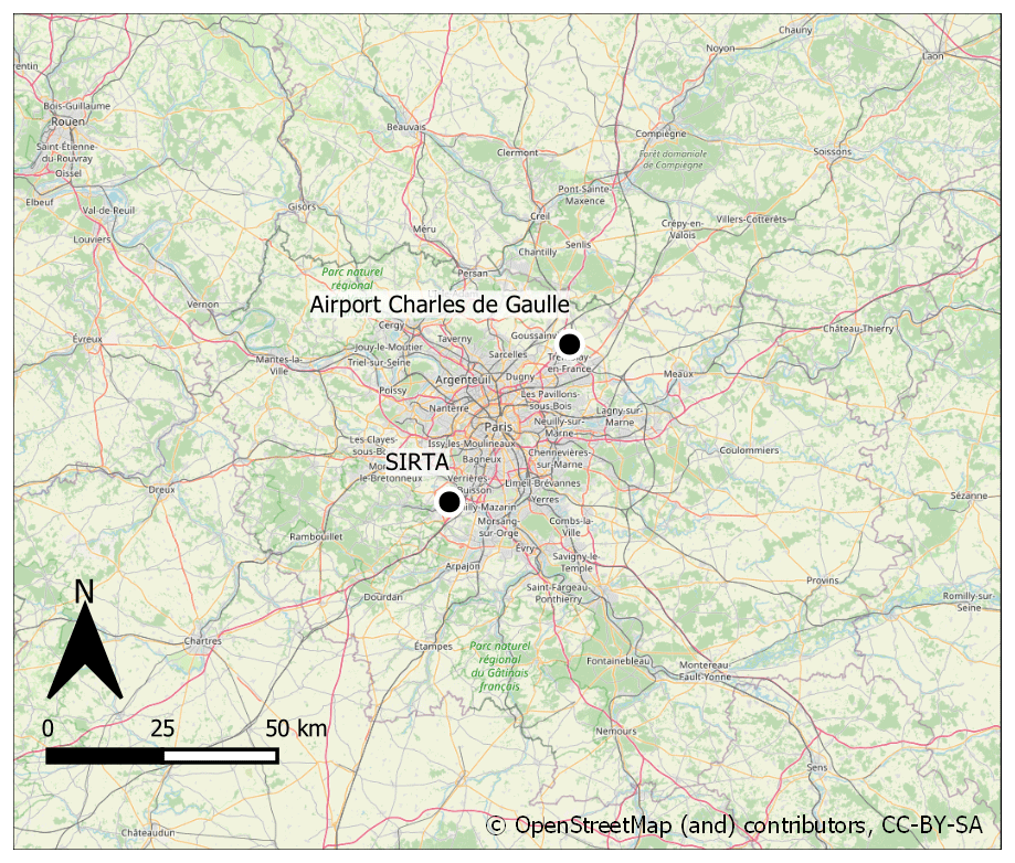
Figure 1 Location of the SIRTA supersite southwest of Paris. © OpenStreetMap contributors 2020. Distributed under a Creative Commons BY-SA License.

2.1 Submicron particle measurements

Aerosol chemical speciation monitor (ACSM;  Ng et al., 2011) measurements are conducted at SIRTA in the framework of the ACTRIS project. The ACSM provides continuous and near-real-time measurements of the major chemical composition of non-refractory submicron aerosols, i.e. organics (Org), ammonium (NH${}_{\mathrm{4}}^{+}$), sulfate (SO${}_{\mathrm{4}}^{\mathrm{2}-}$), nitrate (NO${}_{\mathrm{3}}^{-}$), and chloride (Cl⁻). A detailed description of its functionality can be found in Ng et al. (2011). The data processing and validation protocol can be found in Petit et al. (2015) and Zhang et al. (2019). In addition, black carbon (BC) has been monitored by a seven-wavelength Magee Scientific Aethalometer AE31 from 2011 to mid-2013, and a dual-spot AE33 (Drinovec et al., 2015) from mid-2013 onwards. The consistency of both instruments has been checked in Petit et al. (2014). Using the multispectral information, a differentiation into fossil-fuel-based BC (BCff) and BC from wood burning (BCwb) is achieved (Sciare et al., 2010; Healy et al., 2012; Petit et al., 2014; Zhang et al., 2019). Here, the sum of all measured species is assumed to represent the total PM₁ content (see  Petit et al., 2014, 2015). The consistency of ACSM and Aethalometer measurements is checked by comparing the sum of all monitored species with measurements of a nearby Tapered Element Oscillating Microbalance equipped with a Filter Dynamic Measurement System (TEOM-FDMS). PM₁ measurements are representative of suburban background pollution levels of the region of Paris (Petit et al., 2015). As an additional input to the machine learning model, the average fraction of NO${}_{\mathrm{3}}^{-}$ of the previous day is added (NO3_frac). Pollution events dominated by NO${}_{\mathrm{3}}^{-}$ are often linked to regional-scale events, which depend on anthropogenically influenced processes in the source regions of NO${}_{\mathrm{3}}^{-}$ precursors (Petit et al., 2017). This is approximated by the inclusion of the average fraction of NO${}_{\mathrm{3}}^{-}$ of the previous day, assuming that a high fraction of NO${}_{\mathrm{3}}^{-}$ indicates the occurrence of such an anthropogenically influenced regime.

2.2 Meteorological data

Following the objective of this study, a set of meteorological variables is chosen as inputs for the ML model that either influence PM concentrations directly via dilution (MLH, wind speed (ws), and wet scavenging of particles (precipitation)) and particle transport (wind direction as u, v components, air pressure, AirPres), as a proxy for emissions (e.g. from residential heating: temperature at a height of 2 m (T)), and as a proxy for transformation processes (total incoming solar radiation (TISR), relative humidity (RH), T). Data are taken from the quality-controlled and 1 h averaged re-analysed observation (ReObs) data set. Further information on the instrumentation used for the acquisition of these variables is provided in Chiriaco et al. (2018). MLH is derived from automatic lidar and ceilometer (ALC) measurements of a Vaisala CL31 ceilometer using the CABAM algorithm (Characterising the Atmospheric Boundary layer based on ALC Measurements;  Kotthaus and Grimmond, 2018a, b). Due to an instrument failure, during the period July to mid-November 2016, SIRTA ALC measurements had to be replaced with measurements conducted at the Paris Charles de Gaulle Airport, located northeast of Paris. A comparison of measured MLHs at SIRTA and Charles de Gaulle Airport for the available measurements in 2016 (Appendix A) shows generally good agreement, which is why only minor uncertainties are expected due to the replacement.

Meteorological factors are chosen as input features for the statistical model based on findings of previous studies (see Sect. 1). Meteorological observations are converted to suitable input information for the statistical model (see Sect. 3.1). Wind speed (ws) is derived from the ReObs u and v components [m/s], and the maximum wind speed of the afternoon period (12:00–15:00 UTC) is included in the model. U and v wind components are then normalized to values between 0 and 1, thus only depicting the direction information. To reduce the impact of short-term fluctuation in wind direction, the 3 d running mean is calculated based on the normalized u and v wind components (umean and vmean). Hours since the last precipitation event (Tprec) are counted and used as input to capture the particle accumulation effect between precipitation events (Rost et al., 2009; Petit et al., 2017).

3 Methods

3.1 Machine learning model: technique and application

Gradient boosted regression trees (GBRTs, used here in a Python 3.6.4 environment with the scikit-learn module;  Friedman, 2002; Pedregosa et al., 2012) are applied to predict daily total and speciated PM₁ concentrations. As a tree-based method, GBRTs use a tree regressor, which sets up decision trees based on a training data set. The trees split the training data along decision nodes, creating homogeneous subsamples of the data by minimizing the variance of each subsample. For each subsample, regression trees fit the mean response of the model to the observations (Elith et al., 2008). To increase confidence in the model outputs, decision trees are combined to form an ensemble prediction. Trees are sequentially added to the ensemble (Elith et al., 2008; Rybarczyk and Zalakeviciute, 2018), and each new tree is fitted to the predecessor’s previous residual error using gradient descent (Friedman, 2002). This is an advantage of GBRT over standard ensemble tree methods (e.g. random forests (RF);  Just et al., 2018) as trees are built systematically and fewer iterations are required (Elith et al., 2008). Characteristics of the meteorological training data set with respect to observed total and speciated PM₁ concentrations are conveyed to the statistical model. The learned relationships are then used for model interpretation and to produce estimates of PM₁ based on unseen meteorological data to test the model. The architecture of the statistical model is determined by the hyperparameters, e.g. the number of trees, the maximum depth of each tree (i.e. the number of split nodes on each tree), and the learning rate (i.e. the magnitude of the contribution of each tree to the model outcome, which is basically the step size of the gradient descent). The hyperparameters are tuned by executing a grid search, systematically testing previously defined hyperparameter combinations and determining the best combination via a three-fold cross-validation. Note that PM₁ data are not uniformly distributed; i.e. there are more data available for mid-range PM₁ concentrations. To avoid the model primarily optimizing its predictions on these values, a least-squares loss function was chosen. This loss function is more sensitive to higher PM₁ values (i.e. outliers of the PM₁ data distribution), as it strongly penalizes high absolute differences between predictions and observations. Accordingly, the model is adjusted to reproduce higher concentrations as well. For each PM species, a specific GBRT model is set up and used for the analysis of meteorological influences on individual PM₁ species (see Sect. 4.2). Additionally, a quasi-total PM₁ model is used to reproduce the sum of all species at once, which is used for an analysis of meteorological drivers of high-pollution events (see Sect. 4.3 and 4.4). Train and test data sets to evaluate each model are created by randomly splitting the full data set. These splits, however, are the same for the species models and the full PM₁ model to ensure comparability between the models. Three-quarters of the data are used for training and hyperparameter tuning with cross-validation (n=1086), and one-quarter for testing (n=363). In addition, the robustness of the model results is tested by repeating this process 10 times, resulting in 10 models with different training–test splits and different hyperparameters.

3.2 Explaining model decisions to infer processes: SHapley Additive exPlanation (SHAP) values

While being powerful predictive models, tree-based machine learning methods also have a high interpretability (Lundberg et al., 2020). In order to understand physical mechanisms on the basis of model decisions, the contributions of the meteorological input features to the model outcome are analysed. Feature contributions are attributed using SHAP values, which allow for an individualized, unique feature attribution for every prediction (Shapley, 1953; Lundberg and Lee, 2017; Lundberg et al., 2019, 2020). SHAP values provide a deeper understanding of model decisions than the relatively widely used partial dependence plots (Friedman, 2001; Goldstein et al., 2015; Fuchs et al., 2018; Lundberg et al., 2019; McGovern et al., 2019; Stirnberg et al., 2020). Partial dependence plots show the global mean effect of an input feature to the model outcome, while SHAP values quantify the feature contribution to each single model output, accounting for multicollinearity. Feature contributions are calculated from the difference in model outputs with that feature present, versus outputs for a retrained model without the feature. Since the effect of withholding a feature depends on other features in the model due to interactive effects between the features, differences are computed for all possible feature subset combinations of each data instance (Lundberg and Lee, 2017).

Summing up SHAP values for each input feature at a single time step yields the final model prediction. SHAP values can be negative since SHAP values are added to the base value, which is the mean prediction when taking into account all possible input feature combinations. Negative (positive) SHAP values reduce (raise) the prediction below (above) the base value. The higher the absolute SHAP value of a feature, the more distinct is the influence of that feature on the model predictions. The sum of all SHAP values at one time step yields the final prediction of PM₁ concentrations. An example of breaking down a model prediction into feature contributions using SHAP values is shown schematically in Fig. 2. The computation of traditional Shapley regression values is time consuming, since a large number of all possible feature combinations have to be included. The SHAP framework for tree-based models allows a faster computation compared to full Shapley regression values while maintaining a high accuracy (Lundberg and Lee, 2017; Lundberg et al., 2019) and is therefore used here. The SHAP Python implementation is used for the computation of SHAP values (https://github.com/slundberg/shap, last access: 15 March 2021).

The interactions of input features contribute to the model output and thus reflect empirical patterns that are important to deepen the process understanding. Interactive effects are defined as the difference between the SHAP values for one feature when a second feature is present and the SHAP values for the one feature when the other feature is absent (Lundberg et al., 2019).

Figure 2 Conceptual figure illustrating the interaction of SHAP values and model output. Starting with a base value, which is the mean prediction if all data points are considered, positive SHAP values (blue) increase the final prediction of total and speciated PM₁ concentrations, while negative SHAP values (red) decrease the prediction. The sum of all SHAP values for each input feature yields the final prediction. Depending on whether positive or negative SHAP values dominate, the prediction is higher or lower than the base value (Lundberg et al., 2018). Adapted from https://github.com/slundberg/shap (last access: 15 March 2021).

4 Results and discussion

4.1 Model performance

The performance of the species and total PM₁ models, each with 10 model iterations (of which each has different hyperparameters) is assessed by comparing the coefficient of determination (R²) and normalized root mean square error (NRSME) for the independent test data that were withheld during the training process (Fig. 3). While the models for BCwb, BCff, and total PM₁ show small spread, Cl⁻ and NO${}_{\mathrm{3}}^{-}$ exhibit larger variations between model runs (indicated by horizontal and vertical lines in Fig. 3). This suggests that while drivers of variations in BCff concentration are well covered by the model, this is less so in the case of Cl⁻ and NO${}_{\mathrm{3}}^{-}$. Possible reasons for this are that no explicit information on anthropogenic emissions or chemical formation pathways are included in the models. Still, the model performance indicators highlight that a large fraction of the variations in particle concentrations are explained by the meteorological variables used as model inputs. Performances of model iterations of the species-specific and total PM₁ are generally similar, suggesting a robust model outcome.

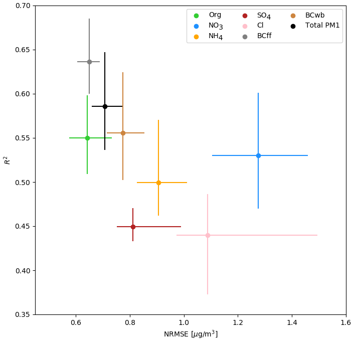
Figure 3 Performance indicators for 10 model iterations: coefficient of determination R² against normalized root mean squared error (NRMSE) for the separate species models (Org: organics, NH${}_{\mathrm{4}}^{+}$: ammonium, SO${}_{\mathrm{4}}^{\mathrm{2}-}$: sulfate, NO${}_{\mathrm{3}}^{-}$: nitrate, Cl⁻: chloride, BCff: black carbon from fossil fuel combustion, and BCwb: black carbon from wood burning), and the total PM₁ model. Vertical and horizontal lines indicate the maximum spread in R² and NRMSE, respectively, between the 10 model iterations.

The mean input feature importance, ordered from high to low, of the total PM₁ model run by means of the SHAP feature attribution values is shown in Fig. 4. The NO${}_{\mathrm{3}}^{-}$ fraction of the previous day has the highest impact on the model, followed by temperature, wind direction information, and MLH. To some extent, NO${}_{\mathrm{3}}^{-}$ fraction can be related to PM₁ mass concentrations (Petit et al., 2015; Beekmann et al., 2015). This means that the higher the PM₁ levels one day, the greater the chances of having higher PM₁ levels the next day (see Fig. B1). Lower wind speeds generally lead to higher particle concentrations (see Fig. B2) due to a lack of dispersion (Sujatha et al., 2016). Temperature, MLH, and wind direction require an in-depth analysis, as changes of these variables cause nonlinear responses in PM₁ predictions, which also vary between species.

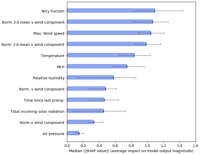
Figure 4 Ranked median SHAP values of the model input features, i.e. the average absolute value that a feature adds to the final model outcome, referring to the total PM₁ model [µg/m³] (Lundberg et al., 2018). Horizontal lines indicate the variability between model runs.

4.2 Influence of meteorological input features on modelled particle species and total PM₁ concentrations

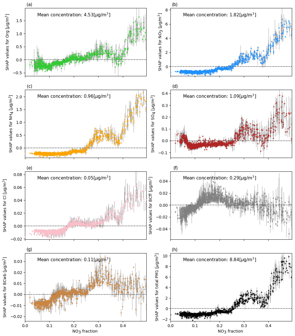
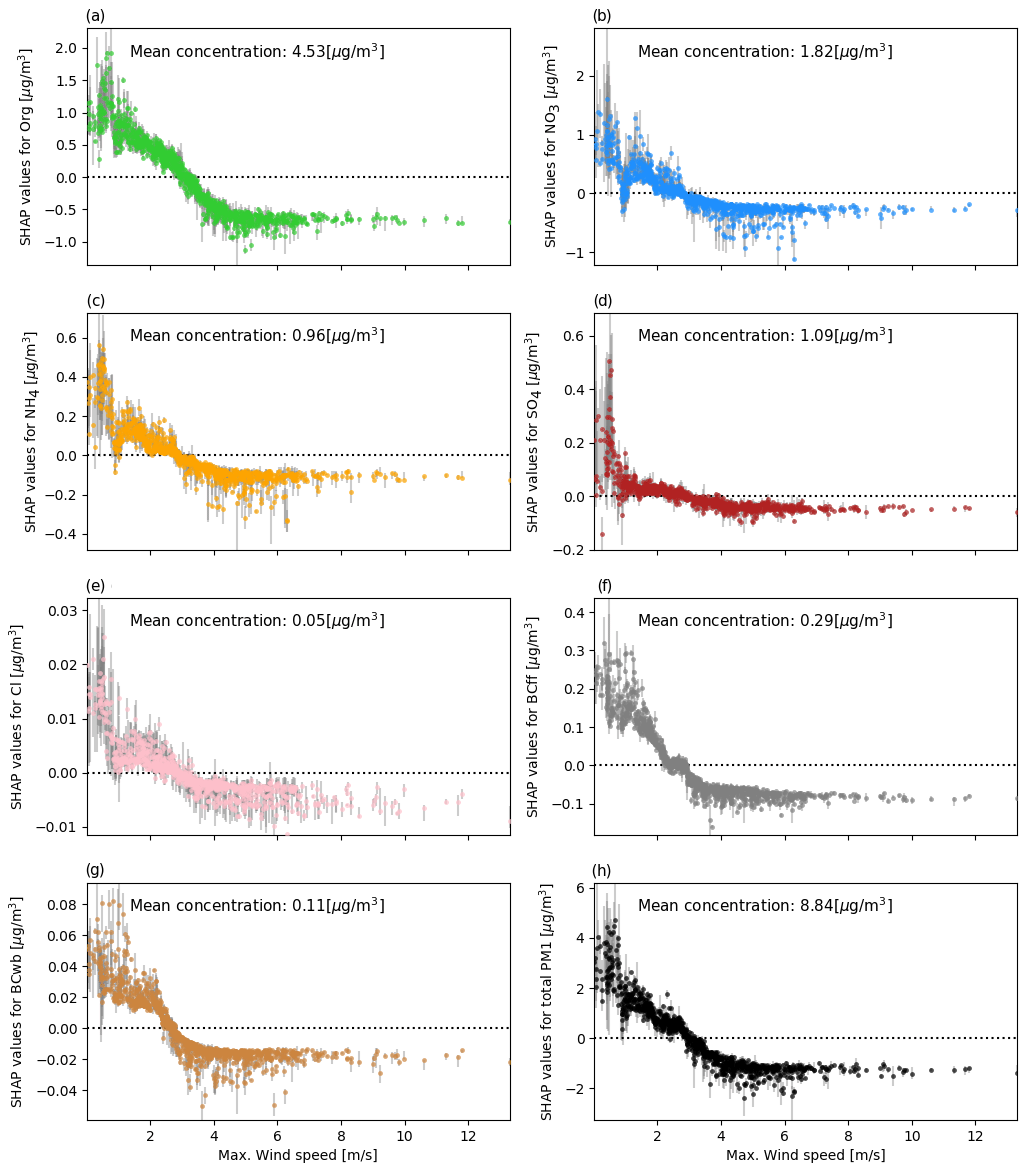
To gain insights into relevant processes governing particle concentrations at SIRTA, the contribution of input features on species and total PM₁ concentration outcomes from the statistical model, i.e. the SHAP values, are plotted as a function of absolute feature values (Figs. 5–7). The contribution of an input feature to each (local) prediction of the species or total PM₁ concentrations is shown while taking into account intra-model variability. Intra-model variability of SHAP values, i.e. different SHAP value attributions for the same feature value within one model, is shown by the vertical distribution of dots for absolute input feature values. Intra-model variability is caused by interactions of the different model input features.

4.2.1 Influence of temperature

The impact of ambient air temperature on modelled species concentrations is highly non-linear (Fig. 5). All species show increased contributions to model outcomes at temperatures below ∼4 ^∘C while the contribution of high temperatures on model outcomes differs substantially between species. The statistical model is able to reproduce well-known characteristics of species concentration variations related to temperature. For example, sulfate formation is enhanced with increasing temperatures (Fig. 5d) due to an increased oxidation rate of SO₂ (see Dawson et al., 2007; Li et al., 2017) and strong solar irradiation due to photochemical oxidation (Gen et al., 2019). Dawson et al. (2007) reported an increase of 34 ng/m³K for PM_2.5 concentrations using a CTM. The increase in sulfate at low ambient temperatures as suggested by Fig. 5d is not reported in this study. It is likely linked to increased aqueous-phase particle formation in cold and foggy situations (Rengarajan et al., 2011; Petetin et al., 2014; Cheng et al., 2016). Considerable local formation of nitrate at low temperatures (Fig. 5b) is consistent with results from previous studies in western Europe, and enhanced formation of ammonium nitrate at lower temperatures (Fig. 5c) by the shifting gas-particle equilibrium is a well-known pattern (e.g. Clegg et al., 1998; Pay et al., 2012; Bressi et al., 2013; Petetin et al., 2014; Petit et al., 2015). The increase in organic matter and BCwb concentrations at low temperatures (Fig. 5g) is likely related to the emission intensity, as biomass burning is often used for domestic heating in the study area (Favez et al., 2009; Sciare et al., 2010; Healy et al., 2012; Jiang et al., 2019). In addition, organic matter concentrations are linked to the condensation of semi-volatile organic species at low temperatures (Putaud et al., 2004; Bressi et al., 2013). The sharp increase in modelled concentrations of organics above 25 ^∘C (Fig. 5a) could be due to enhanced biogenic activity leading to a rise in biogenic emissions and secondary aerosol formation (Guenther et al., 1993; Churkina et al., 2017; Jiang et al., 2019).

The contribution of temperature on modelled total PM₁ concentrations (Fig. 6h) is consistent with the response patterns to changes in temperatures described for the individual species in Fig. 6a–g, with positive contributions at both low (<4 ^∘C) and high air temperatures (>25 ^∘C). For temperatures below freezing, the model allocates maximum contributions to modelled total PM₁ concentrations of up to 12 µg/m³. The spread of SHAP values between model iterations is generally higher for low temperatures (vertical grey bars in Figs. 5–7), where SHAP values are of greater magnitude, but in all cases the signal contained in the feature contributions far exceeds the spread between model runs.

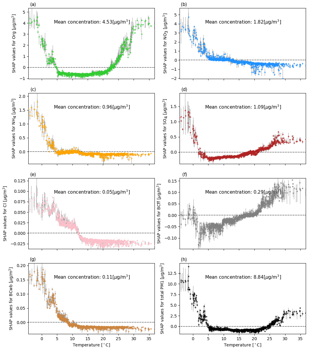
Figure 5 Air temperature SHAP values (contribution of temperature to the prediction of species and total PM₁ concentrations [µg/m³] for each data instance) vs. absolute air temperature [^∘C]. Inter-model variability of allocated SHAP values is shown as the variance of predicted values between the 10 model iterations and plotted as vertical grey bars. The dotted horizontal line indicates the transition from positive to negative SHAP values.

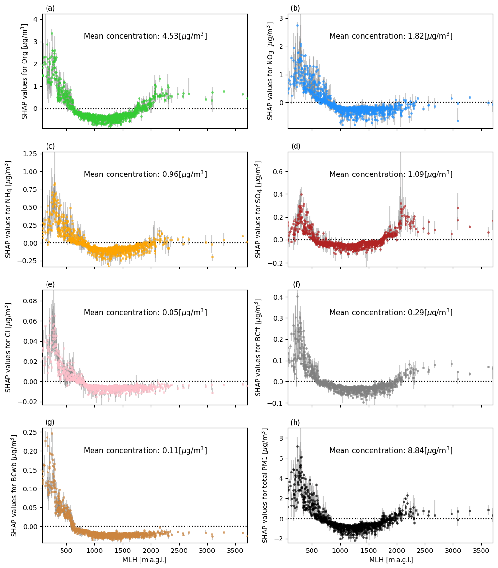
4.2.2 Influence of the mixed layer height (MLH)

Variations in MLH can have a substantial impact on near-surface particle concentrations, as the mixed layer is the atmospheric volume in which the particles are dispersed (see  Klingner and Sähn, 2008; Dupont et al., 2016; Wagner and Schäfer, 2017). The effect of MLH variations on modelled particle concentrations is highly nonlinear and varies in magnitude for all species (Fig. 6). Similar to the patterns observed for temperature SHAP values, the inter-model variation of predictions is highest for low MLHs where predicted particle concentrations have the highest variation. For predicted total PM₁ concentrations, the maximum positive contribution of the MLH is as high as 5.5 µg/m³ while negative contributions can amount to −2 µg/m³. While the maximum influence of MLH is lower than the maximum influence determined for air temperature, the frequency of shallow MLH is far greater than that of the minimum temperatures that have the largest effect (Figs. 5d and 6d). Contributions of MLH to predicted particle concentrations are highest for very shallow mixed layers due to the accumulation of particles close to the ground (Dupont et al., 2016; Wagner and Schäfer, 2017). In addition to causing particles to accumulate near the surface, low MLH can also provide effective pathways for local new particle formation. Secondary pollutants, such as ammonium nitrate, are increased at low MLHs when conditions favourable to their formation usually coincide with reduced vertical mixing (i.e. low temperatures, often in combination with high RH;  Pay et al., 2012; Petetin et al., 2014; Dupont et al., 2016; Wang et al., 2016). BC concentrations, on the other hand, are dominated by primary emissions, as is a substantial fraction of organic matter (Petit et al., 2015). Hence, the accumulation of these particles during low buoyancy conditions can explain the strong influence of MLH on BCwb and BCff. A relatively distinct transition from positive contributions during shallow boundary layer conditions (∼0–800 m) towards negative contributions at high MLHs is evident for all species except SO${}_{\mathrm{4}}^{\mathrm{2}-}$. Modelled SO${}_{\mathrm{4}}^{\mathrm{2}-}$ concentrations show a less distinct response to changes in MLH as they are largely driven by gaseous precursor sources and particle advection, both rather independent of MLH (Pay et al., 2012; Petit et al., 2014, 2015), so that the accumulation effect is less important. The increase of SO${}_{\mathrm{4}}^{\mathrm{2}-}$ concentrations with higher MLHs (≳1500 m a.g.l.) could be linked to the effective transport of SO${}_{\mathrm{4}}^{\mathrm{2}-}$ and its precursor SO₂. In agreement with results from previous studies focusing on PM₁₀ (Grange et al., 2018; Stirnberg et al., 2020) or PM_2.5 (Liu et al., 2018), SHAP values do not change much for MLH above ∼800–900 m; i.e. boundary layer height variations above this level do not influence submicron particle concentrations. Positive contributions of MLHs above ∼800–900 m on predicted PM₁ concentrations, as visible in Fig. 6 for some species, have been previously reported by Grange et al. (2018), who relate this pattern to enhanced secondary aerosol formation in a very deep and dry boundary layer. The positive influence of high MLHs on species that are partly secondarily formed, e.g. SO${}_{\mathrm{4}}^{\mathrm{2}-}$ and Org, could be explained following this argumentation. The increase in SHAP values observed for BCff at high MLHs could be also related to secondary aerosol formation processes, causing an “encapsulation” of BC within a thick coating of secondary aerosols (Zhang et al., 2018).

Figure 6 As Fig. 5 for MLH SHAP values (contribution of MLH to the prediction of species and total PM₁ for each data instance) vs. absolute MLH values [m. a.g.l.].

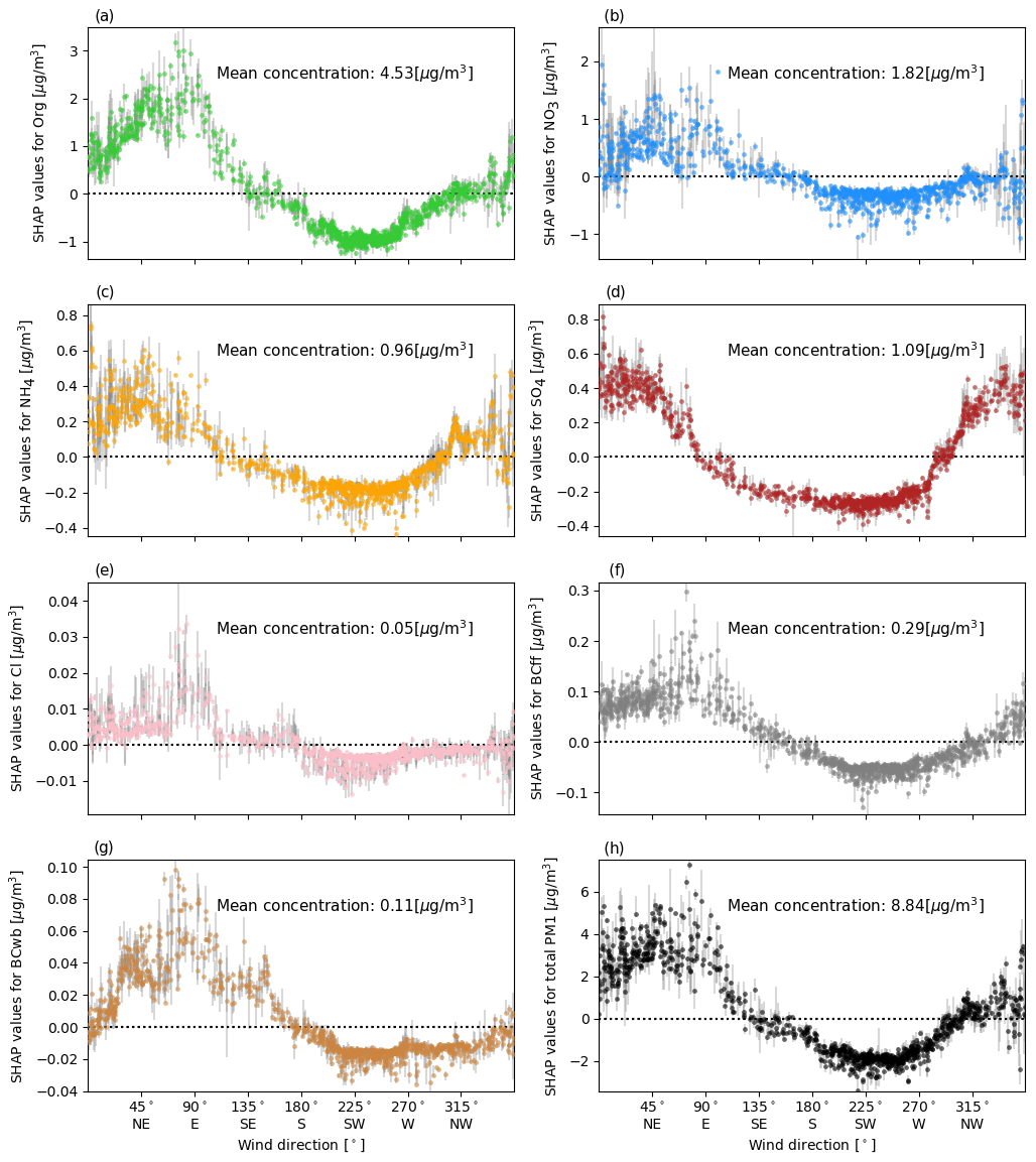
4.2.3 Influence of wind direction

To analyse the contribution of wind direction to predicted particle concentrations, SHAP values of normalized 3 d mean u and v wind components were added up and transformed to units of degrees (Fig. 7). Generally, wind direction has a positive contribution to the model outcome when winds from the northern to northeastern sectors prevail, while negative contributions are evident for southwesterly directions. Given the location of the measurement site, this pattern undoubtedly reflects the advection of particles emitted from continental Europe and/or the Paris metropolitan area under high-pressure system conditions versus cleaner marine air masses during southwesterly flow (Bressi et al., 2013; Petetin et al., 2014; Petit et al., 2015; Srivastava et al., 2018). Increased concentrations of organic matter are predicted for northerly, northeasterly, and easterly winds. These patterns suggest a significant contribution of advected organic particles from a specific wind sector. This is in agreement with the findings of Petetin et al. (2014) who estimated that 69 % of the PM_2.5 organic matter fraction is advected by northeasterly winds, which is related to advected particles from wood burning sources in the Paris region and SOA formation along the transport trajectories. While Petit et al. (2015) did not find a wind direction dependence of organic matter measured at SIRTA using wind regression, they reported the regional background of organic matter to be of importance. Comparing upwind rural stations to urban sites, Bressi et al. (2013) concluded organic matter is largely driven by mid-range to long-range transport. Influences on the SO${}_{\mathrm{4}}^{\mathrm{2}-}$-model are highest for northeastern and eastern wind direction, which aligns with previous findings by Pay et al. (2012), Bressi et al. (2014), and Petit et al. (2017), who identified the Benelux region and western Germany as strong emitters of sulfur dioxide (SO₂). SO₂ can be transformed to particulate SO${}_{\mathrm{4}}^{\mathrm{2}-}$ (Pay et al., 2012) while being transported towards the measurement site. Nitrate concentrations are affected by long-range transport from continental Europe (Benelux, western Germany), which are advected towards SIRTA from northeastern directions (Petetin et al., 2014; Petit et al., 2014). It is to be expected that the influence of mid-range to long-range transport on the particle observations at SIRTA is rather substantial, with most high-pollution days affected by particle advection from continental Europe (Bressi et al., 2013). Concerning BCff and BCwb, model results suggest a dependence on wind direction during northwestern to northeastern inflow. Although BC concentrations are expected to be largely determined by local emissions (Bressi et al., 2013), e.g. from local residential areas, a substantial contribution of imported particles from wood burning and traffic emissions from the Paris region (Laborde et al., 2013; Petetin et al., 2014) and continental sources is likely (Petetin et al., 2014).

Figure 7 As Fig. 5 for wind direction SHAP values (contribution of 3 d mean wind direction to the prediction of species and total PM₁ for each data instance) vs. absolute wind direction [^∘].

4.2.4 Influence of feature interactions

Pairwise interaction effects, where the effect of a specific predictor on the total PM₁ prediction is dependent on the state of a second predictor, are analysed in the model. Strong pairwise interactive effects are found between MLH vs. time since last precipitation and MLH vs. maximum wind speed and shown in Fig. 8a and b. SHAP interaction effects between MLH and time since last precipitation are most pronounced for MLHs below ∼500 m a.g.l. (Fig. 8a). Interaction values are negative for low MLHs paired with time since last precipitation close to zero hours. With increasing time since last precipitation, interaction effects become positive, thus increasing the contribution of Tprec and MLH to the model outcome. An explanation of this pattern concerning underlying processes could be that due to the lack of precipitation, a higher number of particles is available in the atmosphere for accumulation, hence increasing the accumulation effect of a shallow MLH. In case of recent precipitation, the accumulation effect of a shallow MLH is weakened. For higher MLHs, interactive effects with time since the last precipitation event are marginal. Interactive effects between MLH and wind speed are shown in Fig. 8b. Positive SHAP values for maximum wind speeds below ∼2 m/s reflect stable situations, favouring the accumulation of particles, whereas high wind speeds enhance the ventilation of particles (Sujatha et al., 2016). This can also be deduced from Fig. 8b, which shows increased SHAP values for low wind speeds in combination with a low MLH. Low wind speeds combined with a high MLH (≳1000 m a.g.l.), on the other hand, result in decreased SHAP values. Similarly, low MLHs combined with higher wind speeds (≳2 m/s) also decrease predictions of total PM₁ concentrations. High MLHs in combination with high wind speeds, however, reduce SHAP values. A physical explanation of this pattern could be the more effective transport of SO${}_{\mathrm{4}}^{\mathrm{2}-}$ and its precursor SO₂ as well as ammonium nitrate under high-MLH conditions and stronger winds (Pay et al., 2012). Maximum wind speed and time since last precipitation (plot not shown here) interact in a similar way. The positive effect of low wind speeds on the model outcome is increasing with increasing time since last precipitation.

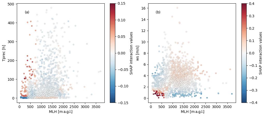
Figure 8 MLH vs. (a) time since last precipitation and (b) maximum wind speed, coloured by the SHAP interaction values for the respective features.

4.3 Meteorological conditions of high-pollution events

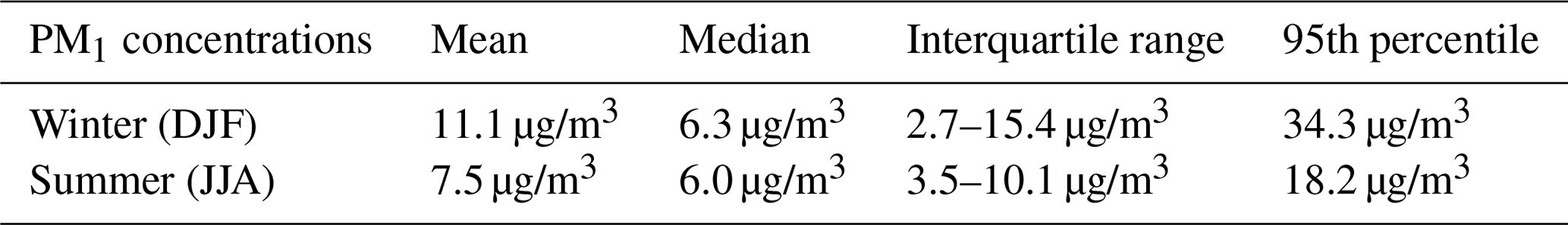
To further identify conditions that favour high-pollution episodes, the data set is split into situations with exceptionally high total PM₁ concentrations (>95th percentile) and situations with typical concentrations of total PM₁ (interquartile range, IQR). This is done for the meteorological summer and winter seasons to contrast dominant drivers between these seasons. Mean SHAP values refer to the total PM₁ model; corresponding input feature distributions and species fractions for the two subgroups are aggregated seasonally. This allows for a quantification of seasonal feature contributions to average or polluted situations.

Table 1 Statistics for typical PM₁ concentrations (mean, median, IQR) and high-pollution concentrations (>95th percentile).

Figures 9 and 10 show mean SHAP values for typical (left) and high-pollution (right) situations in the upper panel. The distribution of SHAP values are shown as box plots for each feature. Absolute feature value distributions are given in the bottom of the figure. In the lowest subpanel, the chemical composition of the total PM₁ concentration for each subgroup is shown. The largest contributor to high-pollution situations in winter is air temperature (Fig. 9). SHAP values for temperature are substantially increased during high-pollution situations, when temperatures are systematically lower. Further contributing factors to high-pollution situations are the low MLHs, low wind speeds, a high average NO${}_{\mathrm{3}}^{-}$ fraction of the previous day, and negative u (i.e. winds from the east) and v (i.e. winds from the north) wind components. In winter, the PM₁ composition shows a relatively large fraction of nitrates, which is increased during high-pollution situations (Fig. 9, lower panel). High concentrations of nitrate in winter can be linked to advection or to enhanced formation due to the temperature-dependent low volatility of ammonium nitrate (Petetin et al., 2014). The organic matter fraction is slightly decreased during high-pollution situations. MLH and maximum wind speed influences on high-pollution situations are linked to low-ventilation conditions which are very frequent in winter (Dupont et al., 2016). Positive influences of wind direction for inflow from the northern and eastern sectors are dominant during high-pollution situations while inflow from the southern and western sectors prevails during average-pollution situations (see Fig. 7;  Bressi et al., 2013; Petetin et al., 2014; Srivastava et al., 2018). Note that the time since the last precipitation is increased during high-pollution situations, but the effects on the model outcome is weak. This suggests that lack of precipitation is not a direct driver of modelled total PM₁ concentrations but increases the contribution of other input features (see Fig. 8a) or is a meaningful factor in only some situations.

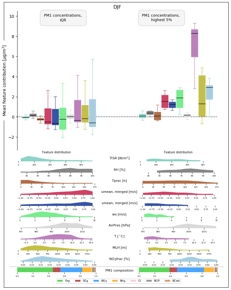
Figure 9 Mean feature contributions (i.e. SHAP values) for situations with low total PM₁ concentrations (left) and situations with high pollution (right), respectively, during winter (December, January, February). Respective ranges of SHAP values by species are shown as box plots, with median (bold line), 25–75th percentile range (boxes), and 10–90th percentile range (whiskers). Both training and test data are included. Absolute feature value distributions (given as normalized frequencies) as well as the chemical composition of the total PM₁ concentration are shown in the subpanels. Colours of the box plots correspond to colours in the feature distribution subpanels. SHAP values of the input features u_norm_3d and u_norm as well as v_norm_3d and v_norm were merged to “u_norm, merged” and “v_norm, merged” to achieve better transparency.

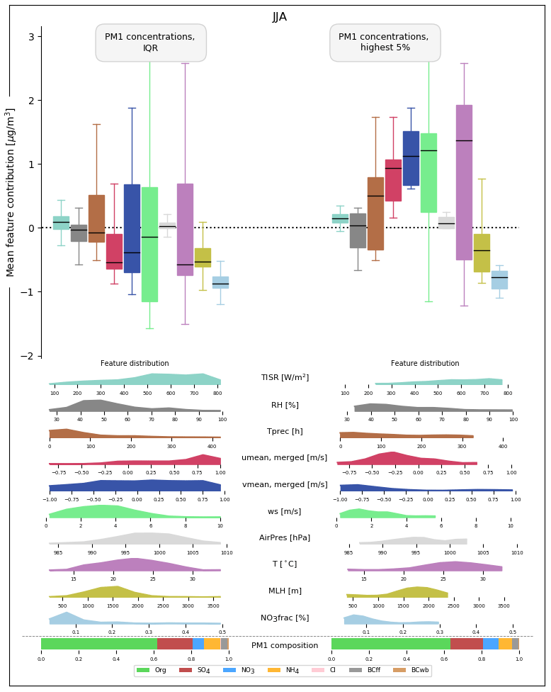
Summer total PM₁ composition (Fig. 10) is characterized by a larger fraction of organics compared to the winter season (Fig. 9). As a considerable fraction of organic matter is formed locally (Petetin et al., 2014), the increased proportion of organics could be due to more frequent stagnant synoptic situations that may limit the advection of transported SIA particles. In addition, the positive SHAP values of solar irradiation and temperature highlight that the solar irradiation stimulates transformation processes and increases the number of biogenic SOA particles (Guenther et al., 1993; Petetin et al., 2014). As mean temperatures are highest in summer, positive temperature SHAP values are associated with increased organic matter concentrations (Fig. 5). The higher importance (i.e. higher SHAP values) of time since the last precipitation event during high-pollution situations points to an accumulation of particles in the atmosphere. Dry situations can also enhance the emission of dust over dry soils (Hoffmann and Funk, 2015). The negative influences of MLH during both typical and high-pollution situations reflects seasonality, as afternoon MLHs in summer are usually too high to have a substantial positive impact on total PM₁ concentrations (see Fig. 6). MLH is thus not expected to be a driver of day-to-day variations of summer total PM₁ concentrations. Note that the average MLH is higher during high-pollution situations, which likely points to increased formation of SO${}_{\mathrm{4}}^{\mathrm{2}-}$ (see Fig. 6).

Figure 10 As Fig. 9 for mean feature contributions (i.e. SHAP values) for situations with low total PM₁ concentrations (left) and situations with high-pollution (right), respectively, during summer (July, June, August).

4.4 Day-to-day variability of selected pollution events

Analysing the combination of SHAP values of the various input features on a daily basis allows for direct attribution of the respective implications for modelled total PM₁ concentrations (Lundberg et al., 2020). Here, four particular pollution episodes are selected to analyse the model outcome with respect to physical processes (Figs. 11–14). The examples highlight the advantages but also the limitations of the interpretation of the statistical model results. The high-pollution episodes took place in winter 2016 (10–30 January and 25 November–25 December), spring 2015 (11–31 March), and summer 2017 (8–28 June).

4.4.1 January 2016

Prior to the onset of the high-pollution episode in January 2016 (Fig. 11), the situation is characterized by MLHs at approximately 1000 m, temperatures above freezing (∼5–10^∘C), frequent precipitation, and winds from the southwest. The organic matter fraction dominates the particle speciation. The episode itself is reproduced well by the model. According to the model results, the event is largely temperature-driven, i.e. SHAP values of temperature explain a large fraction of the total PM₁ concentration variation (note the adjusted y axis of the temperature SHAP values). On 18 January, temperatures drop below freezing, coupled with a decrease in MLH. As a consequence, both modelled and observed PM₁ concentrations start to rise. A further increase in total PM₁ concentrations is driven by a sharp transition from stronger southwestern to weaker northeastern winds (strong negative u component, weak negative v component) on 19 January. The combined effects of these changes lead to a marked increase in total modelled PM₁ concentrations, peaking at ∼37 µg/m³ on 20 January. On the following days, temperatures increase steadily; thus the contribution of temperature decreases. At the same time, although values of MLH remain almost constant, the contribution of MLH drops substantially from ∼5 to ∼2 µg/m³. This is due to interactive effects between MLH and the features wind speed, time since last precipitation, and normalized v wind component. All of these features increase the contribution of MLH on 20 January but decrease its contribution on 21–23 January. The physical explanation behind this pattern would be that a lack of wet deposition and low wind speeds increase particle numbers in the atmosphere, while inflows from northeasterly directions increase particle numbers in the atmosphere. Given that there is now a large number of particles present, the accumulation effect of a low MLH is more efficient. The high-pollution episode ceases after a shift to southeastern winds and the increasing temperatures. The pollution episode is characterized by a relatively large fraction of NO${}_{\mathrm{3}}^{-}$ and NH${}_{\mathrm{4}}^{+}$, which explains the strong feature contribution of temperature to the modelled total PM₁ concentration, as the abundance of these species is temperature dependent (see Fig. 5) and points to a large contribution of locally formed inorganic particles. Still, the contribution of wind direction and speed also suggests that advected secondary particles and their build-up in the boundary layer are relevant factors during the development of the high-pollution episode (Petetin et al., 2014; Petit et al., 2014; Srivastava et al., 2018).

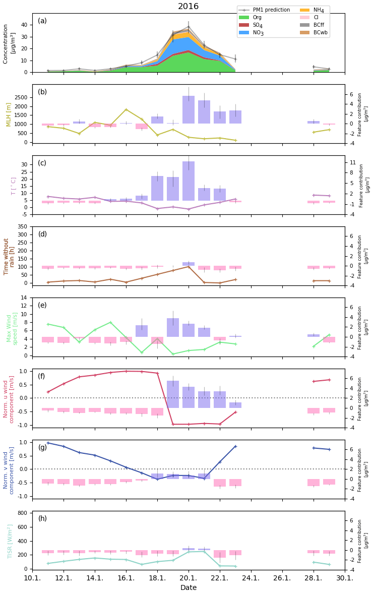
Figure 11 Winter pollution episode in January 2016. Panel (a) indicates the total PM₁ prediction as a horizontal black line with vertical black lines denoting the range of predictions of all 10 models. The observed species concentrations are shown as stacked planes in the corresponding colours. The subsequent panels show absolute values (left y axis, solid lines) and SHAP values (right y axis, pink bars for positive and blue bars for negative values) for the most relevant meteorological input features: MLH (b), temperature (c), hours after rain (d), maximum wind speed (e), normalized u wind (f), and normalized v wind (g) component.

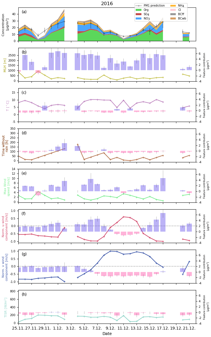
4.4.2 December 2016

A high-pollution episode with several peaks of total PM₁ is observed in November and December 2016. The first peak on 26 November is followed by an abrupt minimum in total PM₁ concentrations on 28 November, and a build-up of pollution in a shallow boundary layer towards the second peak on 2 December with total PM₁ concentrations exceeding 40 µg/m³. In the following days, total PM₁ concentrations continuously decrease, eventually reaching a second minimum on 11 December. A gradual increase in total PM₁ concentrations follows, resulting in a third (double-)peak total PM₁ concentration on 17 December. Total PM₁ concentrations drop to lower levels afterwards. Throughout the 3.5-week-long episode, high pollution is largely driven by shallow MLH (≲500 m) and weak north-northeasterly winds, i.e. a regime of low ventilation associated with high pressure conditions favourable for emission accumulation and possibly some advection of polluted air from the Paris region. During the brief periods with lower total PM₁ concentrations, these conditions are disrupted by a higher MLH (∼28 November) or a change in prevailing winds (∼11 December). In contrast to the pollution episode in January 2016, this December 2016 episode is not driven by temperature changes. Temperatures range between ∼5–12^∘C and have a minor contribution to predicted total PM₁ concentrations (see also Fig. 5), emphasizing the different processes causing air pollution in the Paris region. Note that the model is not able to fully reproduce the pollution peak on 2 December, which may be indicative of missing input features in the model. Judging from the PM₁ species composition during this time (relatively high fraction of NO${}_{\mathrm{3}}^{-}$ and BC), it seems likely that missing information on particle emissions may be the reason for the difference between modelled and observed total PM₁ concentration.

Figure 12 As Fig. 11 for a further winter pollution episode in December 2016.

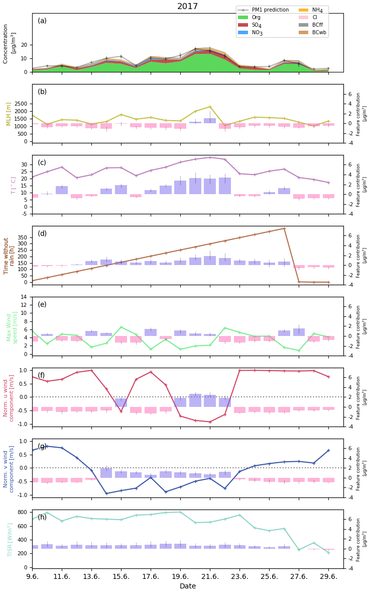
4.4.3 June 2017

A period of above-average total PM₁ concentrations occurred in June 2017. The episode is very well reproduced by the model, suggesting a strong dependence of the observed total PM₁ concentration to meteorological drivers. Although absolute total PM₁ concentrations are substantially lower than during the previously described winter pollution episodes, the event is still above average for summer pollution levels. Organic matter particles dominate the PM₁ fraction throughout the episode, with a relatively high SO${}_{\mathrm{4}}^{\mathrm{2}-}$ fraction. Conditions during this episode are characterized by strong solar irradiation (positive SHAP values) and high MLHs (mostly negative SHAP values), which show low day-to-day variability and reflect characteristic summer conditions. A lack of precipitation (no rain for a period of more than 2 weeks) and high temperatures also contribute to the total PM₁ concentrations during this episode. While solar irradiation and time since last precipitation are associated with positive SHAP values throughout this period, air temperature only has a positive contribution when exceeding ∼25 ^∘C. This aligns with patterns shown in Fig. 5, where increased concentrations of organic matter and SO${}_{\mathrm{4}}^{\mathrm{2}-}$ are identified for high temperatures. Peak total PM₁ concentrations of ∼17 µg/m³ are observed on 20 and 21 June. A change in the east–west wind component from western to eastern inflow directions in conjunction with an increase in temperatures to above 30 ^∘C are the drivers of the modelled peak in total PM₁ concentrations. MLH is also increased with values ∼2000 m a.g.l., which are associated with slightly positive SHAP values. This observation fits with findings described in Sect. 4.2.2 and is likely linked to enhanced secondary particle formation (Megaritis et al., 2014; Jiang et al., 2019). As suggested by response patterns of species to changes in MLH shown in Fig. 7, this effect is linked to an increase in SO${}_{\mathrm{4}}^{\mathrm{2}-}$ concentrations. The main fraction of the peak total PM₁ values, however, is linked to an increase in organic matter concentrations due to the warm temperatures (see Fig. 5).

Figure 13 As Fig. 11 for an exemplary summer pollution episode in June 2017.

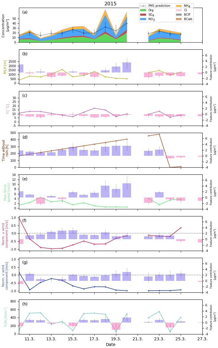
4.4.4 March 2015

High particle concentrations are measured in early March 2015 with high day-to-day variability. This modelled course of the pollution episode is chosen to compare results to previous studies focusing on the evolution of this episode (Petit et al., 2017; Srivastava et al., 2018). The episode is characterized by high fractions of SIA particles, in particular SO${}_{\mathrm{4}}^{\mathrm{2}-}$, NH${}_{\mathrm{4}}^{+}$, and NO${}_{\mathrm{3}}^{-}$ (Fig. 14a) and similar concentrations observed at multiple measurement sites in France (Petit et al., 2017). Contributions of local sources are low, and much of the episode is characterized by winds blowing in from the northwest, advecting aged SIA particles (Petit et al., 2017; Srivastava et al., 2018) and organic particles of secondary origin (Srivastava et al., 2019) towards SIRTA. A widespread scarcity of rain probably enhanced the large-scale formation of secondary pollution across western Europe (in particular western Germany, the Netherlands, Luxemburg;  Petit et al., 2017), which were then transported towards SIRTA. This is reflected by the SHAP values of the u and v wind components, which are positive throughout the episode (see Fig. 14g and h). Concentration peaks of total PM₁ are measured on 18 and 20 March. Both peaks are characterized by a rapid development of total PM₁ concentrations. As described in Petit et al. (2017), these strong daily variations of total PM₁, which are mainly driven by the SIA fraction, could be due to varying synoptic cycles, especially the passage of cold fronts. The influence of MLH and temperature is relatively small, which is consistent with the high influence of advection on total PM₁ concentrations during the episode. The exceptional character of the episode (see Petit et al., 2017) partly explains the bad performance of the model in capturing total PM₁ variability during the event. An unusual rain shortage is observed in large areas of western Europe prior to the episode (Petit et al., 2017). While time since precipitation at the SIRTA site is a large positive contributor to the model outcome (see Fig. 14d), it is not driving the day-to-day variations. The unusual nature of this event and lack of information on emission in the source regions and formation processes along air mass trajectories in the model likely explain why the model has difficulties in reproducing this pollution episode. While this has implications for the application of explainable machine learning models for rare events, this is not expected to be an issue for the other cases and seasonal results presented here.

Figure 14 As Fig. 11 for an exemplary spring pollution episode in March 2015.

5 Conclusions and outlook

In this study, dominant patterns of meteorological drivers of PM₁ species and total PM₁ concentrations are identified and analysed using a novel, data-driven approach. A machine learning model is set up to analyse measured speciated and total PM₁ concentrations based on meteorological measurements from the SIRTA supersite, southwest of Paris. The machine learning model is able to reproduce daily variability of particle concentrations well and is used to analyse and quantify the atmospheric processes causing high-pollution episodes during different seasons using a SHAP-value framework. As interactions between the meteorological variables are accounted for, the model enables the separation, quantification, and comparison of their respective impacts on the individual events. It is shown that ambient meteorology can substantially exacerbate air pollution. Results of this study point to the distinguished role of shallow MLHs, low temperatures, and low wind speeds during peak PM₁ episodes in winter. These conditions are often amplified by northeastern wind inflow under high-pressure synoptic circulation. A detailed analysis reveals how the meteorological drivers of winter high-pollution episodes interact. For an episode in January 2016, model results show a strong influence of temperature to the elevated PM₁ concentrations during this episode (up to 11 µg/m³ are attributed to temperature), suggesting enhanced local, temperature-dependent particle formation. During a different, prolonged pollution episode in December 2016, temperature levels were relatively stable and had no influence. Here, MLH (<500 m a.s.l.) was quantified to be the main driver of modelled PM₁ peak concentrations with contributions up to 6 µg/m³, along with wind direction contributions of up to ∼6 µg/m³. Total PM₁ concentrations in spring can be as high as 50 µg/m³. These peaks in spring are not as well reproduced by the model as winter episodes and are likely due to new particle formation processes along the air mass trajectories, in particular of nitrate. Summer PM₁ concentrations are lower than in other seasons. Model results suggest that summer peak concentrations are largely driven by high temperatures, particle advection from Paris and continental Europe with low wind speeds, and prolonged periods without precipitation. For an example episode in June 2017, temperatures above 30 ^∘C contribute ∼3 µg/m³ to the total PM₁ concentration. On-site scarcity of rain increases air pollution but does not appear to be a major driver of strong day-to-day variations in particle concentrations. Presumably, this is because droughts are synoptic and are spread over several days or even weeks. Thus, they present very low inter-daily variability on the local scale. Nonetheless, Petit et al. (2017) have highlighted the link between extreme PM concentrations (especially during spring) and extreme precipitation deficit (compared to average conditions). The main drivers of day-to-day variability of predicted PM₁ concentrations are changes in wind direction, air temperature, and MLH. These changes often superimpose the influence of time without precipitation. Individual PM₁ species are shown to respond differently to changes in temperature. While SO${}_{\mathrm{4}}^{\mathrm{2}-}$ and organic matter concentrations are increased during both high- and low-temperature situations, NH${}_{\mathrm{4}}^{+}$ and NO${}_{\mathrm{3}}^{-}$ are substantially increased only at low temperatures. Model results indicate that SIA particle formation is enhanced during shallow MLH conditions. The presented findings refer to the SIRTA supersite but the results are nevertheless transferable to other regions as well. For example, the importance of temperature-induced particle formation processes have been shown for the USA (Dawson et al., 2007), Europe (Megaritis et al., 2014), and China (Wang et al., 2016). Hence, it is likely that the detailed, species-dependent disclosure of the nonlinear relationship between temperature and PM₁ of this study holds for other urban and suburban areas. This has implications for the PM concentrations in the context of climate change. The empirical perspective of the current study complements the findings of various modelling studies (Dawson et al., 2007; Megaritis et al., 2013, 2014; Sá et al., 2016; Doherty et al., 2017); the insights provided here from an empirical perspective could increase the confidence in air quality estimations under climate change. Furthermore, the impact of shallow MLHs on PM₁ concentrations investigated here is comparable to results found in a previous, regional-scale study over central Europe that highlighted the dominant role of MLH on PM₁₀ concentrations (Stirnberg et al., 2020). The importance of wind direction highlights the role of advected pollution by remote, highly polluted urban or industrial hotspots. In general, the interpretation of pollution advection patterns requires knowledge on source regions and terrain. Here, the Paris agglomeration is a major source of pollutants while the relatively flat terrain allows unimpeded advection of air masses. Urban areas in a more complex terrain would likely be affected by slightly different and possibly more complex mechanisms, such as terrain- and meteorology-dependent air stagnation events Wang et al. (2018) as well as orography-driven wind and precipitation patterns (Rosenfeld et al., 2007). Still, given the task of disentangling the impact of the various meteorological drivers on air quality is already a complex scientific subject, a continental, flat terrain city such as Paris was chosen as the subject area precisely to exclude other factors (such as orographic flow or sea breeze) that would add further complexity. Certainly, the methods developed here could be transferred to other urban areas in more complex settings in the framework of future studies.

Furthermore, the analysis of meteorological drivers could be extended in future studies, e.g. by including information on anthropogenic emissions or further stations down- and upwind of SIRTA, which would allow further analysis of dominant advection patterns. Furthermore, information on emissions or meteorology in the source region of air masses, e.g. using satellite-based observations, might be helpful to better reproduce particle transport patterns. This could be complemented by incorporating synoptic variables, e.g. the North Atlantic Oscillation (NAO) index.

For policy makers, the presented approach could prove beneficial in multiple ways. Knowledge of meteorological conditions that exacerbate air pollution could be used to issue preventative warnings to the public if these conditions are forecasted. Another potential future application could be the quantitative assessment of policy measures, e.g. traffic bans, by comparing an “expected” level of air pollution under given meteorological conditions to actual observations (e.g.  Cermak and Knutti, 2009). Finally, the presented model framework could be combined with short-term weather forecasts, which would allow an air quality forecast based on the predictions of the statistical models to be provided.

Appendix A: Comparison of mixed layer height (MLH) measured at SIRTA and Charles de Gaulle airport

As mentioned in Sect. 2.2, ca. 90 missing MLH values in 2016 were replaced with measurements conducted at the Charles de Gaulle airport (see Fig. 1). Figures A1 and A2 summarize MLH values for 2016 when measurements from both sites are available (afternoon period). As shown in Fig. A1, measurements at both sites generally agree well, except for some outliers. Spearman's rank coefficient is significant (p value < 0.05) and has a value of 0.51.

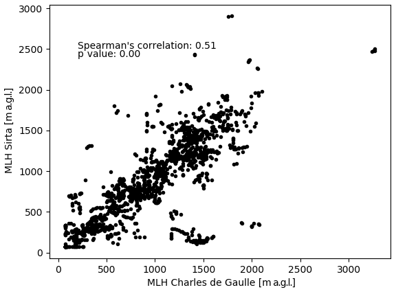
Figure A1 Scatterplot for MLH [m a.g.l.] measured at SIRTA vs. MLH measured at Charles de Gaulle airport.

A comparison of the frequency of occurrence is shown as histogram in Fig. A1 and indicates good agreement as well.

Figure A2 Histogram showing the frequency of occurrence for MLH [m a.g.l.] measured at SIRTA (red) vs. MLH measured at Charles de Gaulle airport (black).

Appendix B: Illustration of the influence of NO${}_{\mathrm{3}}^{-}$ fraction and wind speed

Figures B1 and B2 illustrate the influence of the NO${}_{\mathrm{3}}^{-}$ fraction and maximum wind speed on the model outcome using SHAP values.

Figure B1 As Fig. 5 for fraction of NO${}_{\mathrm{3}}^{-}$ SHAP values (contribution of NO${}_{\mathrm{3}}^{-}$ fraction to the prediction of species and total PM₁ for each data instance) vs. absolute NO${}_{\mathrm{3}}^{-}$ fraction.

Figure B2 As Fig. 5 for the maximum wind speed SHAP values (contribution of maximum wind speed to the prediction of species and total PM₁ for each data instance) vs. absolute maximum wind speed.