the Creative Commons Attribution 4.0 License.
the Creative Commons Attribution 4.0 License.
 | 11 Mar 2021
Influence of the El Niño–Southern Oscillation on entry stratospheric water vapor in coupled chemistry–ocean CCMI and CMIP6 models
Chaim I. Garfinkel
Ohad Harari
Shlomi Ziskin Ziv
Olaf Morgenstern
Guang Zeng
Simone Tilmes
Douglas Kinnison
Fiona M. O'Connor
Neal Butchart
Makoto Deushi
Patrick Jöckel
Andrea Pozzer
Sean Davis
The connection between the dominant mode of interannual variability in the tropical troposphere, the El Niño–Southern Oscillation (ENSO), and the entry of stratospheric water vapor is analyzed in a set of model simulations archived for the Chemistry-Climate Model Initiative (CCMI) project and for Phase 6 of the Coupled Model Intercomparison Project. While the models agree on the temperature response to ENSO in the tropical troposphere and lower stratosphere, and all models and observations also agree on the zonal structure of the temperature response in the tropical tropopause layer, the only aspect of the entry water vapor response with consensus in both models and observations is that La Niña leads to moistening in winter relative to neutral ENSO. For El Niño and for other seasons, there are significant differences among the models. For example, some models find that the enhanced water vapor for La Niña in the winter of the event reverses in spring and summer, some models find that this moistening persists, and some show a nonlinear response, with both El Niño and La Niña leading to enhanced water vapor in both winter, spring, and summer. A moistening in the spring following El Niño events, the signal focused on in much previous work, is simulated by only half of the models. Focusing on Central Pacific ENSO vs. East Pacific ENSO, or temperatures in the mid-troposphere compared with temperatures near the surface, does not narrow the inter-model discrepancies. Despite this diversity in response, the temperature response near the cold point can explain the response of water vapor when each model is considered separately. While the observational record is too short to fully constrain the response to ENSO, it is clear that most models suffer from biases in the magnitude of the interannual variability of entry water vapor. This bias could be due to biased cold-point temperatures in some models, but others appear to be missing forcing processes that contribute to observed variability near the cold point.
- Article
(7576 KB) - Full-text XML
-
Supplement
(2468 KB) - BibTeX
- EndNote


Water vapor is the gas with most important greenhouse effect in the atmosphere, and the feedback associated with stratospheric water vapor in response to increasing anthropogenic greenhouse gas emissions is around half of that for global mean surface albedo or cloud feedbacks (Forster and Shine, 1999; Solomon et al., 2010; Dessler et al., 2013; Banerjee et al., 2019; Li and Newman, 2020). The amount of water vapor entering the stratosphere also regulates the severity of ozone depletion (Solomon et al., 1986) and is important for other aspects of stratospheric chemistry (Dvortsov and Solomon, 2001). Hence, it is important to understand how the comprehensive models that are used for projections of future ozone and climate capture the processes regulating the entry of stratospheric water vapor.
Lower-stratospheric water vapor concentrations are mainly determined by the tropical temperatures near the cold point, where dehydration takes place as air parcels transit into the stratosphere (Mote et al., 1996; Zhou et al., 2004, 2001; Fueglistaler and Haynes, 2005b; Fueglistaler et al., 2009; Randel and Park, 2019). Several different processes have been shown to influence these cold-point temperatures, and the goal of this work is to revisit the influence of one of these processes – the El Niño–Southern Oscillation (ENSO) – on entry water vapor in the lower stratosphere.
El Niño (EN), the ENSO phase with anomalously warm sea surface temperatures in the tropical East Pacific, leads to a warmer tropical troposphere and cooler tropical lower stratosphere (Free and Seidel, 2009; Calvo et al., 2010; Simpson et al., 2011), with the zero-crossing in the vicinity of the cold point (Hardiman et al., 2007). In addition, EN leads to a zonal dipole in temperature anomalies near the tropopause and, in particular, to a Rossby wave response with anomalously warm temperatures over the Indo-Pacific warm pool and anomalously cold temperatures over the Central Pacific (Yulaeva and Wallace, 1994; Randel et al., 2000; Zhou et al., 2001; Scherllin-Pirscher et al., 2012; Domeisen et al., 2019). In the tropical tropopause layer (TTL), water vapor increases in the region with warm anomalies and decreases in the region with cold anomalies by ∼25 % (Gettelman et al., 2001; Hatsushika and Yamazaki, 2003; Konopka et al., 2016).
The net effect of these zonally asymmetric and symmetric changes on water vapor above the tropical cold point is complex. The two largest EN events in the satellite era (in 1997–1998 and in 2015–2016) were followed by moistening of the tropical lower stratosphere (Fueglistaler and Haynes, 2005a; Avery et al., 2017; Diallo et al., 2018), and the ERA5 reanalysis, which tracks satellite water vapor well over the last few decades, also shows a clear moistening after the 1982–1983 event (Fig. 3 of Wang et al., 2020). Strong La Niña (LN) events in 1998–1999 and 1999–2000 also clearly preceded elevated water vapor concentrations in the tropical lower stratosphere. The net effect of more moderate events (either LN or EN) is unclear (Gettelman et al., 2001), and there may be a nonlinear effect. Specifically, Garfinkel et al. (2018) found that both strong EN and LN events lead to elevated water vapor concentrations compared with neutral ENSO in a chemistry–climate model, and indeed such an effect is weakly evident (although not significant) in observations (Fig. 4 of Garfinkel et al., 2018). In addition, there is a strong seasonal dependence of the effect of EN on stratospheric water vapor, with the increase in water vapor for EN and decrease for LN occurring mainly in boreal spring (Calvo et al., 2010; Garfinkel et al., 2013; Konopka et al., 2016; Tao et al., 2019).
The limited duration of the observational data record, and the importance of other atmospheric processes (e.g., the quasi-biennial oscillation), which may interact nonlinearly with ENSO (Yuan et al., 2014), limit the confidence with which observed variability during and following ENSO events can be unambiguously associated with ENSO. Several studies have used simulations from single models to try to understand the role of ENSO with respect to entry stratospheric water vapor (Scaife et al., 2003; Garfinkel et al., 2013; Brinkop et al., 2016; Garfinkel et al., 2018; Ding and Fu, 2018), although it is not clear whether the results are general to other models. The goal of this study is to consider a wider range of models, with a combined model output of over 2700 years, in order to better understand the response of stratospheric water vapor to ENSO. We focus here on chemistry–climate models, as these models must reasonably simulate entry water vapor, otherwise their stratospheric chemistry will suffer from biases.
After introducing the data and methodology in Sect. 2, we contrast the impact of ENSO on stratospheric water vapor in 12 different chemistry–climate models. Even though all models simulate a similar response to ENSO in the troposphere and also in the lower stratosphere (warming and cooling, respectively), there is no consensus as to the impact of ENSO on stratospheric water vapor. Some models simulate enhanced water vapor for EN in both the winter of the event and the following spring, some models find an opposite response, and some simulate a nonlinear response, with both EN and LN leading to enhanced water vapor in spring (as is evident in GEOSCCM, Garfinkel et al., 2018). In all cases, the temperature response near the cold point can explain the divergent responses of water vapor to ENSO.
2.1 Data
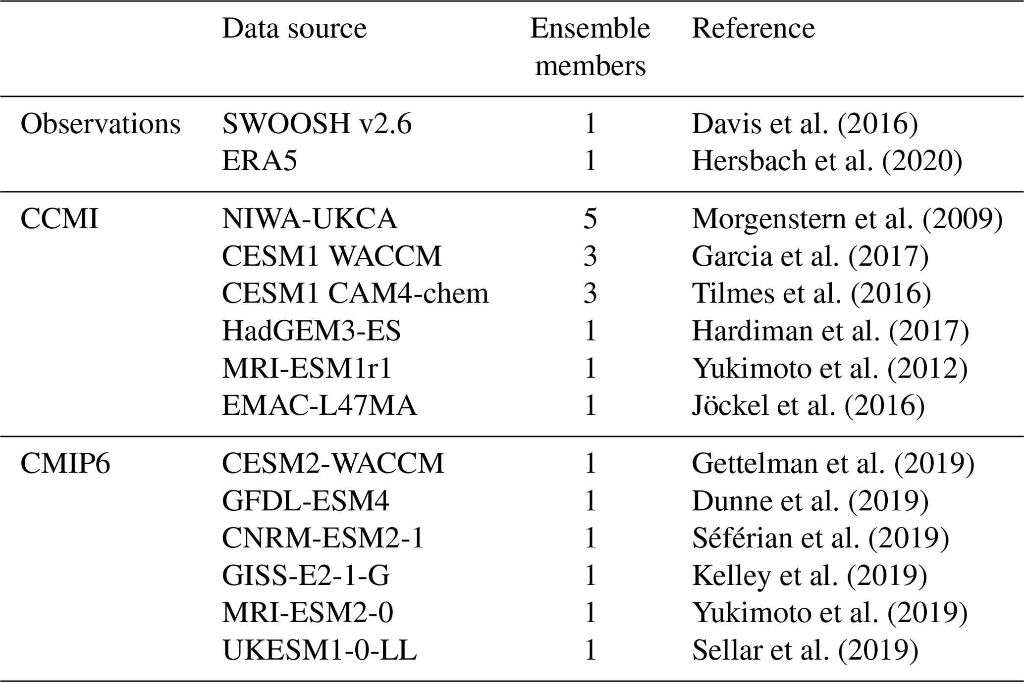
We examine six models participating in the Chemistry-Climate Model Initiative (CCMI; Morgenstern et al., 2017) and six models participating in Phase 6 of the Coupled Model Intercomparison Project (CMIP6; Eyring et al., 2016). However, the focus in most of this paper is on the CCMI models, for which data are archived at a higher vertical resolution, as this allows for a more careful diagnosis of the physical processes. Coupled chemistry–climate models are expected to have more robust interannual variability in temperatures in the lower stratosphere compared with models with fixed ozone (Yook et al., 2020); hence, we only include CMIP6 models with interactive stratospheric chemistry.
CCMI was jointly launched by the Stratosphere-troposphere Processes And their Role in Climate (SPARC) and the International Global Atmospheric Chemistry (IGAC) projects to better understand chemistry–climate interactions in the recent past and future climate (Eyring et al., 2013; Morgenstern et al., 2017). This modeling effort is an extension of CCMVal2 (SPARC-CCMVal, 2010), but it utilizes up-to-date chemistry–climate models that also include tropospheric chemistry. We consider the Ref-C2 simulations, which span the 1960–2100 period, impose ozone-depleting substances reported by the World Meteorological Organization (2011), and impose greenhouse gases other than ozone-depleting substances as in Representative Concentration Pathway (RCP) 6.0 (Meinshausen et al., 2011). The full details of these simulations are described by Eyring et al. (2013). Note that the GEOSCCM simulations provided to CCMI did not have a coupled ocean, but Garfinkel et al. (2018) have already examined the ENSO–water vapor connection in this model in a coupled ocean configuration. As we are interested in connections between ENSO and the stratosphere, we only consider CCMI models with a coupled ocean in which ENSO develops spontaneously. We consider all available ensemble members. The CCMI models used in this study are listed in Table 1. Harari et al. (2019) showed that each of these models simulates surface temperature variability in the Nino3.4 region similar to that observed.
In addition to the CCMI models, we also consider six Earth system models with coupled chemistry that are participating in CMIP6: CESM2-WACCM (Gettelman et al., 2019), GFDL-ESM4 (Dunne et al., 2019), CNRM-ESM2-1 (Séférian et al., 2019), GISS-E2-1-G (Kelley et al., 2019), MRI-ESM2-0 (Yukimoto et al., 2019), and UKESM1-0-LL (Sellar et al., 2019). The seasonal cycle and climatology of stratospheric water vapor for five of these models is documented in Keeble et al. (2020). For these models, we focus on the historical integrations of the period from 1850 to 2014. Note that standard CMIP6 output includes the 70 and 100 hPa levels but no level in between, which limits our ability to diagnose physical processes near the cold point. (In contrast, CCMI output is available both near 80 and 90hPa.) All of the CCMI models and all of the CMIP6 models except GISS-E2-1-G represent the quasi-biennial oscillation (QBO) (Rao et al., 2020a; Richter et al., 2020; Rao et al., 2020b). In total, more than 2700 years of model output are available.
Davis et al. (2016)Hersbach et al. (2020)Morgenstern et al. (2009)Garcia et al. (2017)Tilmes et al. (2016)Hardiman et al. (2017)Yukimoto et al. (2012)Jöckel et al. (2016)Gettelman et al. (2019)Dunne et al. (2019)Séférian et al. (2019)Kelley et al. (2019)Yukimoto et al. (2019)Sellar et al. (2019)Table 1The data sources used in this study. For CMIP6 models, we focus on the historical integrations of the period from 1850 to 2014; for CCMI, we focused on the Ref-C2 simulations spanning the period from 1960 to 2100.
Model output is compared to model-level temperatures in the ERA5.1 reanalysis (Hersbach et al., 2020) and water vapor from 1993 through 2019 in version 2.6 of the SWOOSH dataset (specifically the combinedeqfillanomfill product, Davis et al., 2016). ERA5 assimilates available satellite and GPS data in the tropical tropopause layer and has a higher vertical resolution (approximately 300 m in the tropical tropopause layer) than any previous reanalyses (Hersbach et al., 2020).
Table 2Note that the pressure level for each model differs due to data availability, and the levels used for this chart are indicated in Fig. 2.
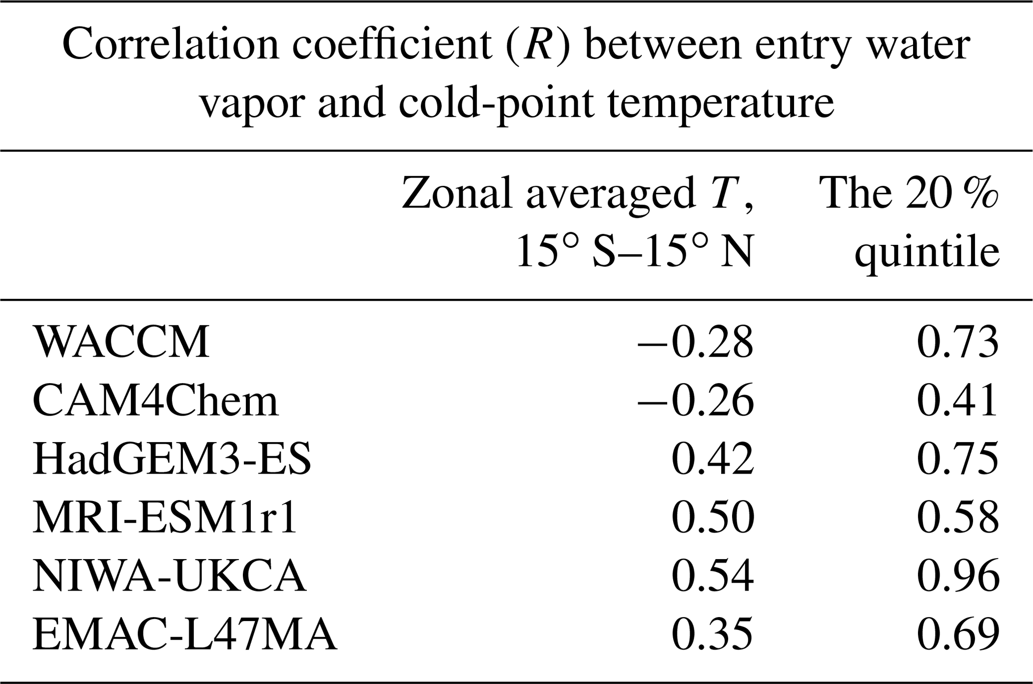
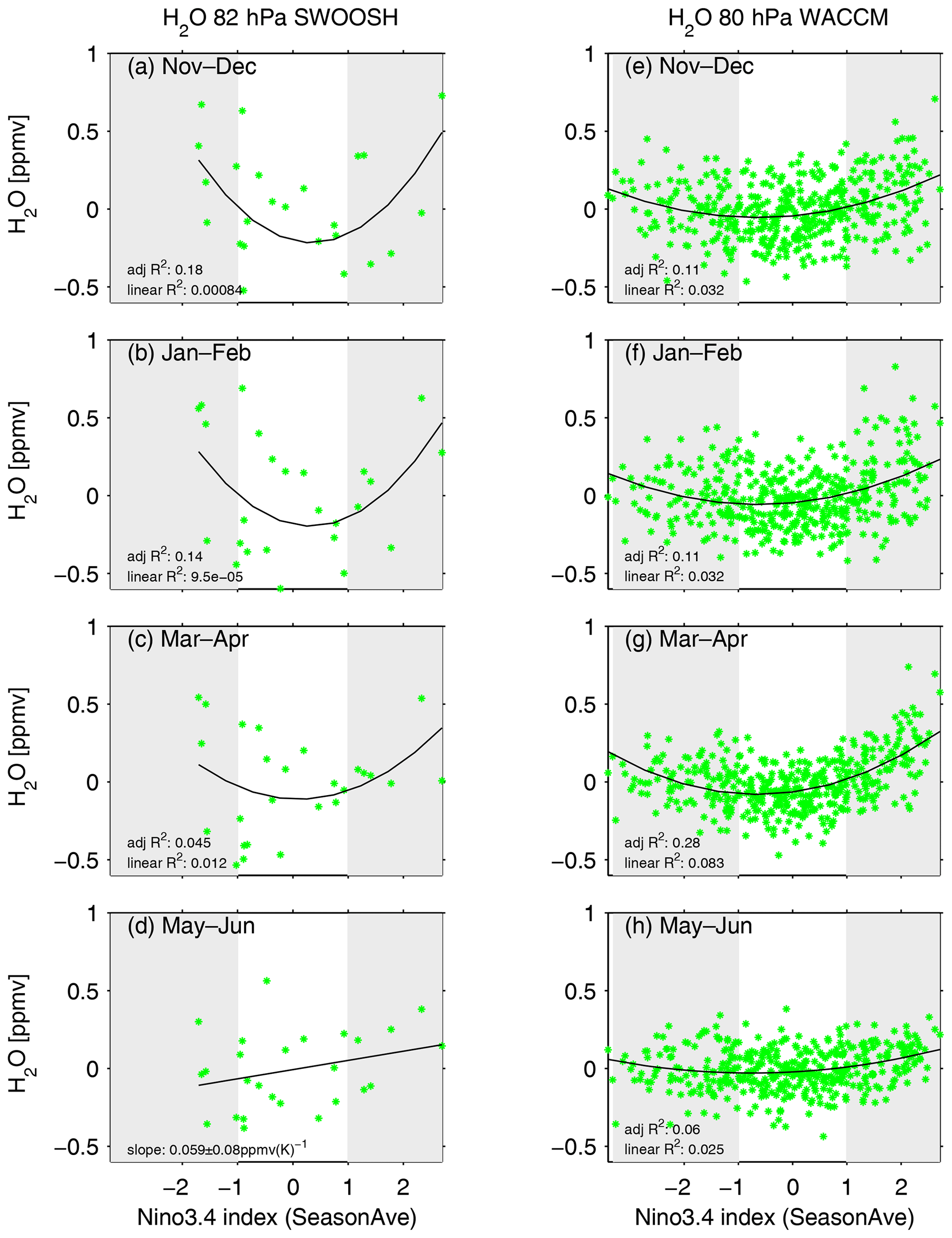
Figure 1Anomalous 80 hPa water vapor in WACCM compared with the value of the Nino3.4 index for (a) November and December, (b) January and February, (c) March and April, and (d) May and June. Each dot corresponds to 1 model year. When a polynomial fit better describes the dependence on ENSO than a linear fit, we show the R2 for a linear fit and the adjusted R2 for the polynomial fit (see Sect. 2.2). Otherwise we show a linear least squares best fit in each panel.
2.2 Methods
This study focuses on the impact of ENSO on the stratosphere on interannual timescales; in order to remove any impacts on longer timescales due to climate change and also to remove any linear impacts from the quasi-biennial oscillation, which is known to affect water vapor (Reid and Gage, 1985; Zhou et al., 2001, 2004; Fujiwara et al., 2010; Liang et al., 2011; Kawatani et al., 2014; Brinkop et al., 2016), we first use multiple linear regression (MLR) to remove the linear variability associated with greenhouse gases and the QBO from all time series (i.e., the same regression is applied to temperature and water vapor). We use historical CO2 concentrations for historical simulations and the equivalent CO2 from the RCP6.0 scenario to track future greenhouse gas concentrations (Meinshausen et al., 2011) as well as zonal averaged zonal winds from 5∘ S to 5∘ N at 50 hPa with a 2-month lag to track the QBO. We compute the QBO separately for each data source. Tao et al. (2019) found a maximum correlation for a 1-month lag, whereas we find the correlation is higher for a longer lag (not shown), although our conclusions are unchanged if we use 1 month. For consistency, this same MLR procedure is applied to CCMI, CMIP6, and ERA5/SWOOSH data.
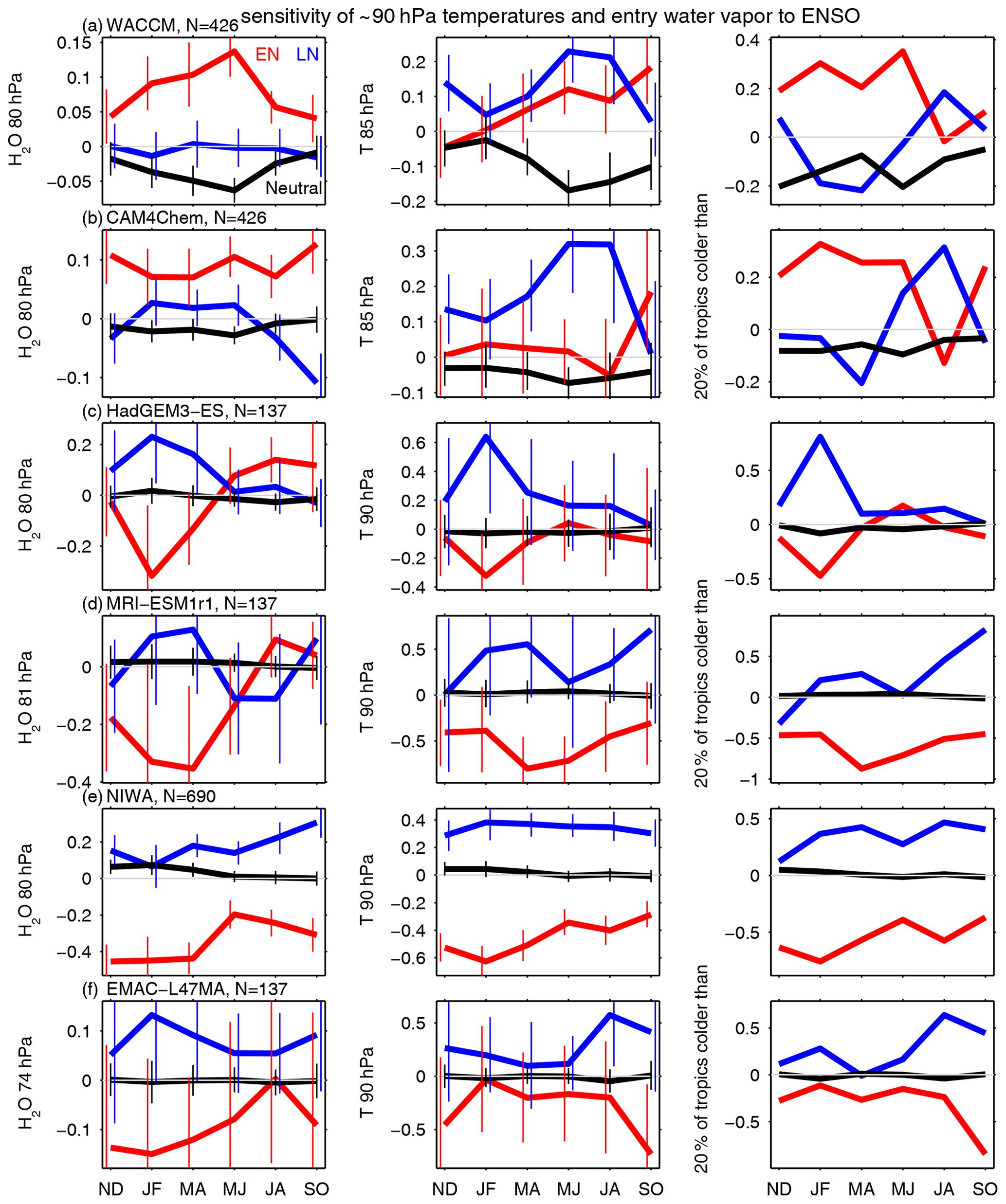
Figure 2Tropical water vapor from 15∘ S to 15∘ N near 80 hPa in each of the six CCMI models considered here from the late fall as the event is developing through to the following summer for (red) El Niño, (blue) La Niña and (black) neutral ENSO (left column). The 5 % confidence intervals on the anomalous response based on a two-tailed Student's t test are shown. The response of zonally averaged temperature anomalies from 15∘ S to 15∘ N near 90 hPa for each model (middle column). The evolution of the temperature of the coldest 20 % of the tropics at 90 hPa for each model in each ENSO phase compared with the model's climatology (right column).
Each CCMI model makes data available at different pressure or sigma levels, which limits the precision with which we can compare models. However, differences in the pressure levels at which data are available are generally less than 2 hPa, and we consider anomalies of each model from its own climatology. When considering entry water vapor for CCMI, we examine the level closest to 80 hPa, and when considering the cold-point temperature, we examine the level closest to 90 hPa archived by each CCMI model. The specific levels chosen for each CCMI model are indicated in the figures.
For ENSO, we use surface air temperature in the region bounded by 5∘ S–5∘ N and 190∘ E–240∘ E (i.e., the Nino3.4 region), as sea surface temperature was not available for all models at the time we downloaded the data. A composite of EN events is formed if the average temperature in the Nino3.4 region in November through February (NDJF) relative to each model's climatology exceeds 1 K, whereas a composite of LN events is formed if the average temperature anomaly is less than −1 K. All other years are categorized as neutral ENSO. A typical ENSO event slowly strengthens in the summer and fall, reaches its maximum strength in late fall or early winter, and then decays in the spring (Fig. 1 of Wang and Fiedler, 2006). This evolution is captured in the models (Fig. S1 in the Supplement). While the influence of ENSO on tropospheric temperatures is rapid due to convection, there is a lag of a few months in the transport from the level with peak convective outflow to the cold point (Mote et al., 1996; Fueglistaler et al., 2004). However, the sea surface temperature anomalies due to ENSO are already established by fall; hence, all of the anomalies shown here are associated with ENSO.
Statistical significance of the composite mean response to a given ENSO phase is determined using a Student's t test. The adjusted R2 (Eq. 3.30 of Chatterjee and Hadi, 2012) is used to quantify the added value in using a polynomial best fit (e.g., H2O ) instead of a linear best fit (e.g., H2O ). The adjusted R2 considers the likelihood that a polynomial predictor will reduce the residuals by unphysically over-fitting the data. The polynomial fit can be preferred if the adjusted R2 for the polynomial fit is larger by any amount compared with the linear R2, although we only show the polynomial fit if the adjusted R2 exceeds the R2 for a linear fit by 33 %. Note that the 33 % criterion is subjectively chosen, although results are similar for a slightly modified criterion.
We begin with the water vapor response to ENSO in the WACCM simulation included in CCMI in Fig. 1. At 90 hPa and also at higher pressure levels (i.e., lower in the TTL), EN leads to enhanced water vapor and LN leads to reduced water vapor in both winter and spring. Convection can rapidly mix moist boundary layer air with the TTL (e.g., Levine et al., 2007). Above the cold point, however, the water vapor response is not significant in November and December, but it then shows a distinct nonlinearity in subsequent months, with both EN and LN leading to enhanced water vapor. This nonlinear effect is similar to that seen in the GEOSCCM model by Garfinkel et al. (2018) and is also similar to the effect in SWOOSH observational data (Fig. 1).
These results are summarized in Fig. 2a, which shows the water vapor response for EN (the events in the right shaded box in Fig. 1), LN (the events in the left shaded box in Fig. 1), and neutral ENSO (all other events). In January through June, both EN and LN lead to significantly more entry water vapor than neutral ENSO. The pronounced moistening during EN peaks in the spring after the event has already begun to decay. These effects are all consistent with that seen in GEOSCCM in Garfinkel et al. (2018). A generally similar effect is evident in CAM4Chem, which shares code with WACCM.
The four models shown in Fig. 2c, d, e, and f have a qualitatively different response to ENSO than the NCAR models and GEOSCCM. Specifically, HadGEM3-ES, NIWA, MRI-ESM1r1, and EMAC-L47MA all simulate somewhat more water vapor for LN than neutral ENSO (although this effect is generally not statistically significant), and significantly more water vapor for neutral ENSO than EN, in January through April. In NIWA and EMAC-L47MA this effect extends through all calendar months.
This large diversity in the entry water vapor response to ENSO occurs despite the fact that all models simulate a qualitatively similar response in tropospheric and lower-stratospheric temperatures, as we now demonstrate.
Figure 3 shows the distribution of 15∘ S–15∘ N temperature as a function of longitude and height for these six models in March and April, the months with the strongest disparity among the models in the response of entry water to ENSO, and a map view of the temperature anomalies at 100 and 70 hPa are included in the Supplement.
All models are characterized by a more pronounced tropospheric warming between 200∘ E and 250∘ E immediately above the region with warming sea surface temperatures compared with other longitudes, and there is a zonal mean increase in temperature throughout the troposphere in all models. The tropospheric warming peaks in the upper troposphere and extends up to the TTL near 120∘ E in all models. Furthermore, all models simulate a lower-stratospheric cooling (above 70 hPa) in response to EN and a warming in response to LN. While the magnitude of these features differs among the model, the patterns are robust.
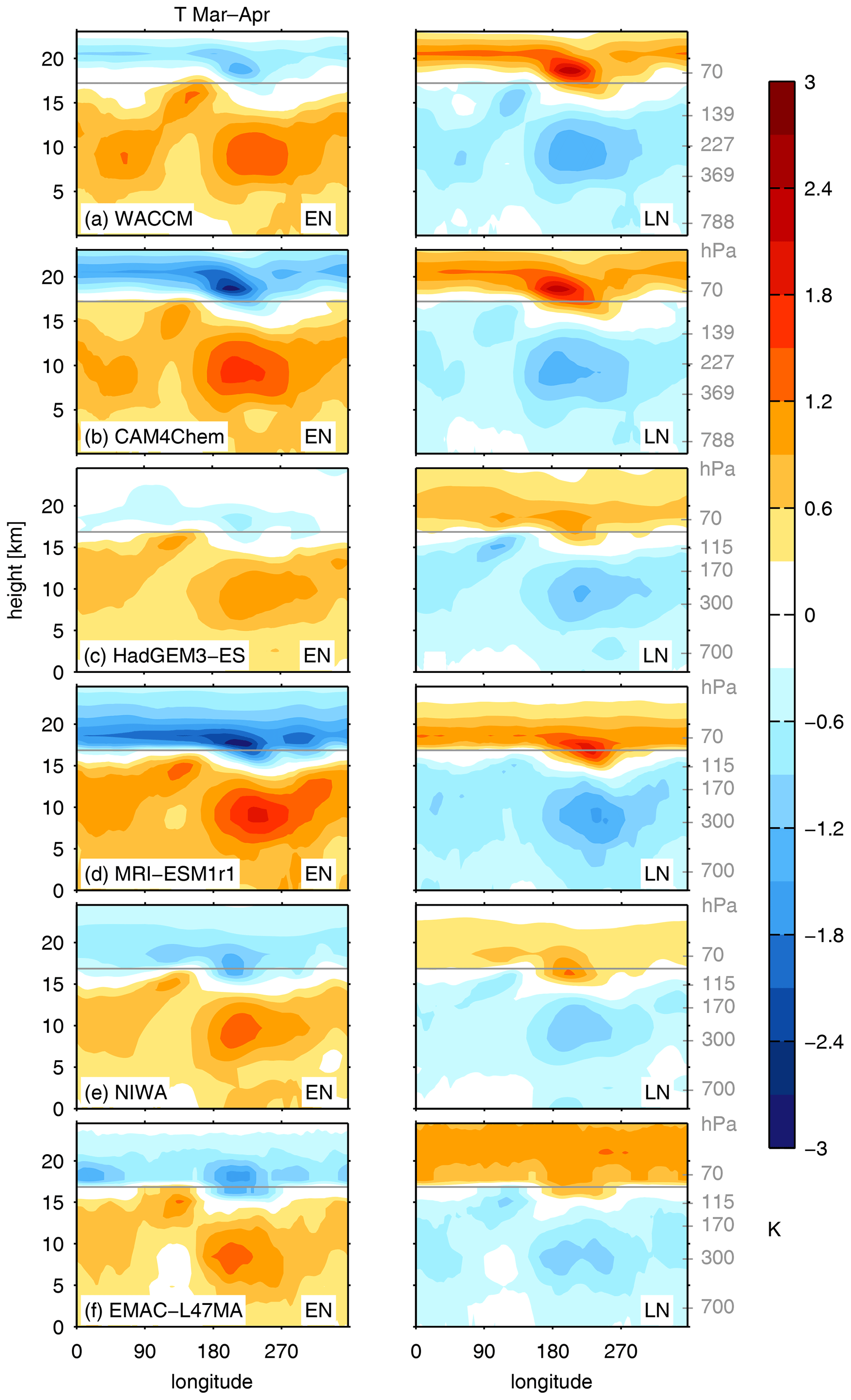
Figure 3Longitude vs. height cross section of the 15∘ S–15∘ N temperature anomalies during (left) El Niño and (right) La Niña in each of the CCMI models. The Supplement presents map views of temperature anomalies at 70 and 100 hPa.
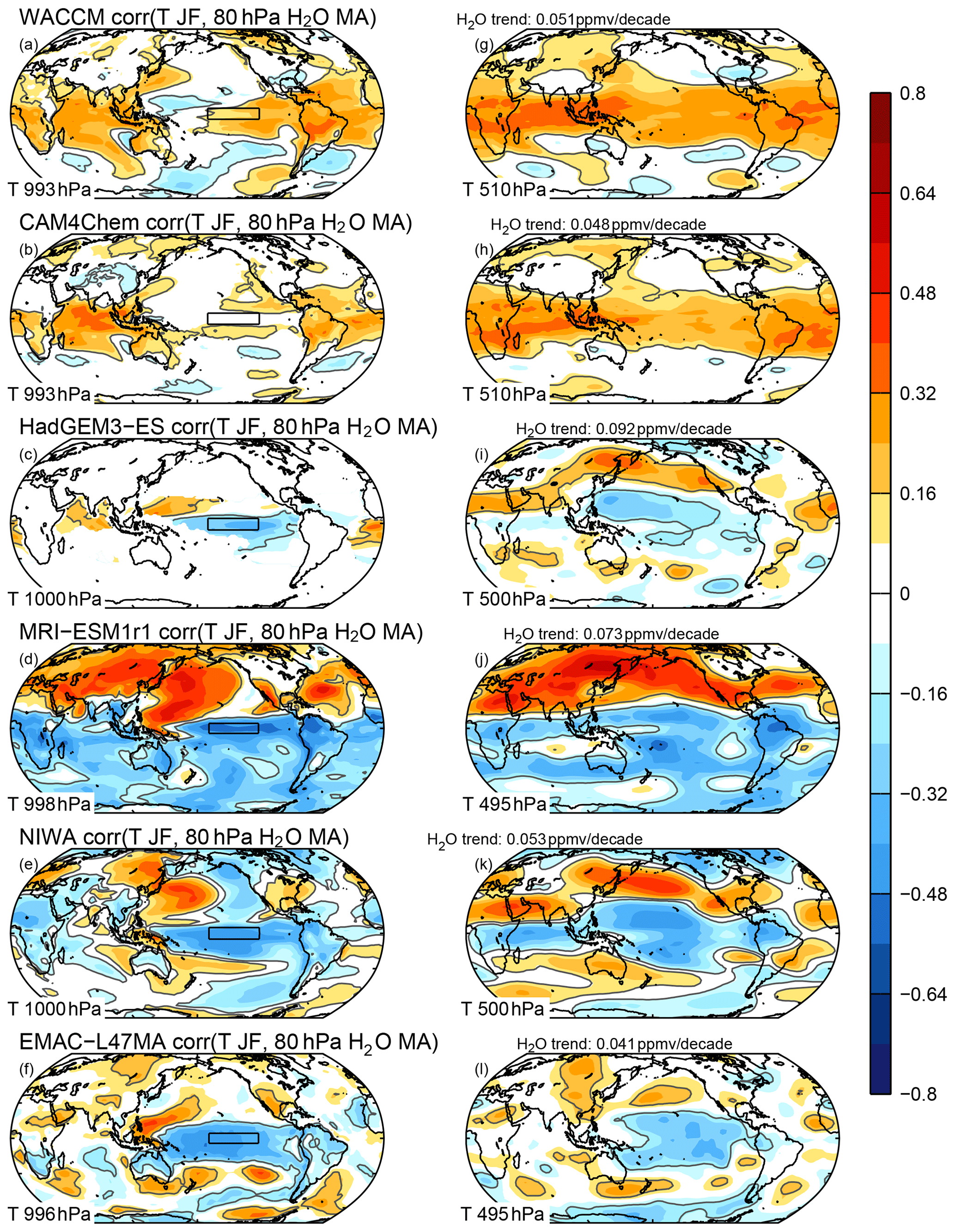
Figure 4Correlation of (left) near-surface temperature and (right) temperature near 500 hPa with entry water vapor in each of the CCMI models, with temperature taken for January and February and water vapor for March and April. A black line indicates correlations significantly different from zero at the 95 % confidence level.
Near the tropopause, however, there is less agreement among the models in the large-scale temperature response, and this difference can account for the large diversity in the water vapor responses to ENSO. The middle column of Fig. 2 shows the zonally averaged temperature response to ENSO in the tropics near 90 hPa. The zonally averaged temperature response to ENSO in WACCM has little resemblance to the water vapor response. Rather, the water vapor response can be better understood by focusing on the coldest region of the tropics. Due to the relative slowness of vertical transport compared with horizontal transport in the tropical tropopause layer, entry water vapor is sensitive to the coldest regions in the tropics and not just zonal mean temperatures (i.e., the cold point; Mote et al., 1996; Hatsushika and Yamazaki, 2003; Bonazzola and Haynes, 2004; Fueglistaler et al., 2004; Fueglistaler and Haynes, 2005a; Oman et al., 2008; Randel and Park, 2019). We quantify this effect as follows: we first sort the temperature in all grid points from 15∘ S to 15∘ N in each bimonthly period; we then calculate the threshold temperature associated with the first quintile, second quintile, etc., of tropical temperatures; we compute these quintiles separately for the EN, LN, and neutral ENSO composites and then compute the difference for each composite from the model climatology. The results of this analysis for the second quintile are shown in the right column of Fig. 2a. The coldest 20 % of the tropics is ∼ 0.25 K warmer during EN compared with the model climatology from November through June, whereas the coldest 20 % of the tropics is colder than the model climatology for LN and neutral ENSO. Overall, the correlation between the 20 % quintile cold-point temperature anomalies and the water vapor anomalies is 0.73 (Table 2). Results are generally similar for CAM4Chem through June: the correlation of entry water with the coldest 20 % is positive, whereas the correlation with zonal mean temperatures is not.
HadGEM3-ES, NIWA, MRI-ESM1r1, and EMAC-L47MA all simulate similar temperature responses if we focus on the zonal mean or the coldest 20 % of the tropics, although correlations with entry water vapor are higher if we focus on the coldest 20 % of the tropics rather than zonal mean temperature (Table 2). For these models, temperatures are warmer for LN than neutral ENSO and colder for EN than neutral ENSO (Table 2). Overall, the temperature response to ENSO in the coldest 20 % of the tropics near 90 hPa can help account for the substantial inter-model diversity in the response of entry water to the stratosphere.
Garfinkel et al. (2013) and Ding and Fu (2018) considered the possibility that sea surface temperatures (SSTs) in the Central Pacific may have a different effect on entry water than SSTs in the East Pacific, and the two studies, using different individual models, found that warmer SSTs in the Central Pacific lead to dehydration. We evaluate this effect for the CCMI models in Fig. 4. Specifically, the left column of Fig. 4 shows the correlation between entry water in March and April and near-surface temperature in January and February. There is clearly a wide range of responses evident, and consistent with Fig. 2, some models show a positive correlation between SSTs in the Nino3.4 region (e.g., WACCM) whereas others show a negative correlation (HadGEM3-ES, NIWA, MRI-ESM1r1, and EMAC-L47MA). There is no clear difference in the correlation between near-surface temperature to the east or west of the Nino3.4 region (indicated with a black box in Fig. 4), and there is clearly no consensus among the models as to whether warmer SSTs in the Central Pacific lead to dehydration.
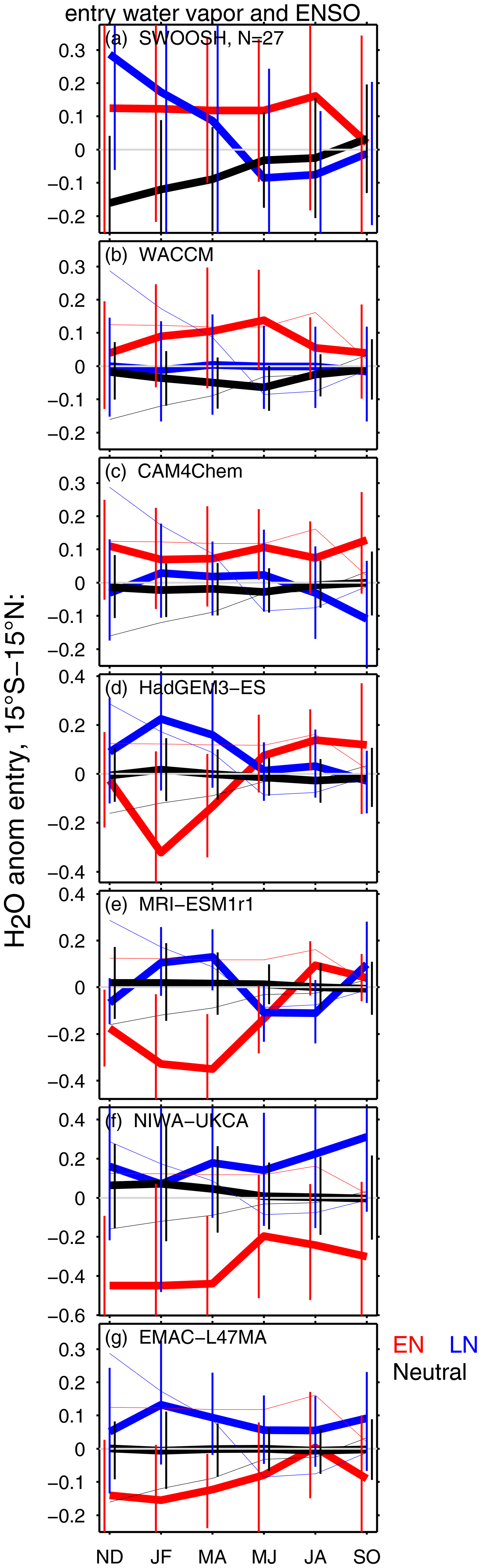
Figure 5(a) As in Fig. 2a but for SWOOSH at 82 hPa. (b–g) As in Fig. 2 but subsampling the model output for each model to match the sample size in observations for each ENSO phase. The uncertainty (marked with vertical lines) of the model response is determined by Monte Carlo subsampling, as described in the text. The response in Fig. 2a is repeated with a thin line in subsequent panels.
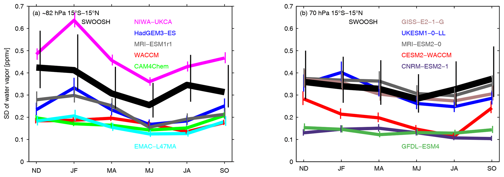
Figure 6Standard deviation of tropical entry water vapor for each model in (a) CCMI near 82 hPa and (b) CMIP6 at 70 hPa as well as for SWOOSH water vapor (thick line). The vertical lines denote the 95 % confidence bounds, as discussed in the text.
Dessler et al. (2013) and Dessler et al. (2014) find that tropical tropospheric temperatures at 500 hPa are a better predictor of entry water vapor than ENSO in the satellite record. Therefore, we consider the correlation between entry water in March and April and 500 hPa temperature in January and February for each model in Fig. 4 (right column). There is clearly a wide range of responses evident, and the response is similar in pattern to that in Fig. 4a–f. Specifically, some models show a positive correlation of entry water with mid-tropospheric temperatures (e.g., WACCM and CAM4Chem) whereas others show a negative correlation (HadGEM3-ES, NIWA, MRI-ESM1r1, and EMAC-L47MA). Note that all models simulate a long-term moistening trend of the lower stratosphere if the trend is computed before applying the MLR described in Sect. 2 (trend indicated above Fig. 4g, h, i, j, k, and l), and of the six models considered, the two with the strongest long-term moistening trend simulate a negative correlation between temperatures at 500 hPa and entry water vapor when focusing on interannual variability. Hence, there is no evidence that temperatures at 500 hPa are a more discriminatory predictor of entry water vapor on interannual timescales than ENSO. Results are similar if we allow for a 4-month lag between tropospheric temperature and entry water vapor for five of the six models (Fig. S4). That being said, it is conceivable that on longer timescales, the magnitude of mid-tropospheric warming would be, for example, related to an upward expansion of the TTL (a robust response to climate change), and such an expansion of the TTL might be expected to lead to more entry water vapor. A thorough investigation of this possibility is beyond the scope of this paper.
What is the observed response of entry water vapor to ENSO? Figure 5a is the same as Fig. 2a but for SWOOSH entry water vapor, and while both LN and EN are associated with more water vapor, the difference between EN and neutral ENSO and between LN and neutral ENSO is not statistically significant. (Note that if ERA5.1 water vapor is used and the years 1979 to 2019 are considered, the moistening for EN is significant in July and August.) Similarly, the regression coefficient of a linear best fit of entry water vapor with ENSO (Fig. 1) is also not statistically significant (and for ERA5.1 water vapor, the increase is significant in July and August; details are not shown). Despite the lack of a significant effect in observations, the models that appear to be closest to the observed response are the NCAR models and also the GEOSCCM simulations evaluated by Garfinkel et al. (2018).
A complication when comparing the models to SWOOSH entry water is that ∼ 140 years at least of model data are available for each model, whereas only 27 years of data are available for observations. Hence, it is ambiguous whether the difference between models and observations reflects an actual model bias or, alternately, might reflect uncertainty given the small observational sample (i.e., the large error bars in Fig. 5a overlap the error bars in Fig. 2 for many models). In order to better compare model and observations, we adopt a Monte Carlo subsampling technique. Taking EN as an example, we randomly select six EN events from each model to match the number of observed EN events in the SWOOSH period, and we compute the mean entry water vapor anomaly for these events. We then repeat this random sampling 2000 times with different EN events randomly included in the subsample. Finally, we compute the top and bottom 2.5 % quantiles of the subsampled response to EN, to which we can compare the observed response.
Figure 5b–g show the response to ENSO in these subsamples for each model, and we repeat the observed response with a thin line. If the observed response falls outside of the middle 95 % of the subsampled response (indicated with a vertical line), the model response to ENSO is inconsistent with that observed. There is a lack of overlap of the subsamples of the model with the observed response for at least one season or phase for all modeling centers. For some of the CCMI models, the degree of inconsistency is relatively small. Specifically, the response in HadGEM3-ES, WACCM, and CAM4Chem is consistent with observations in most seasons and for most phases, with gaps between the vertical bars and the observed response generally being small (Fig. 5b, c, d). The other models, however, suffer from large discrepancies between the observed and modeled responses to ENSO even when we compare similar sample sizes.
An additional metric to evaluate differences in observed vs. modeled ENSO teleconnections is for the model to simulate a similar amount of variance compared with that observed, as otherwise the model does not satisfactorily capture internal atmospheric variability (Deser et al., 2017; Garfinkel et al., 2019; Weinberger et al., 2019). Therefore, we compare the standard deviation of entry water vapor for each model in Fig. 6a. The 95 % confidence interval of the standard deviation as given by a chi-square test is indicated with a vertical line. In boreal winter, only HadGEM3-ES and MRI-ESM1r1 simulate realistic variability, with NIWA simulating too much and the other models simulating too little. In boreal summer, all models suffer from unrealistic variability.
Recently, at least six coupled ocean–chemistry–climate models have participated in CMIP6, and we now assess the ENSO–water vapor connection in the following models: CESM2-WACCM, GFDL-ESM4, GISS-E2-1-G, MRI-ESM2-0, UKESM1-0-LL, and CNRM-ESM2-1. Of these six models, three are newer versions or successors of models that participated in CCMI (CESM2-WACCM, MRI-ESM2-0, and UKESM1-0-LL). Figure 7 is the same as Fig. 5 but for 70 hPa water vapor, as water vapor near 80 hPa is not a standard CMIP6 output variable. The observed water vapor response at 70hPa resembles that at 82 hPa (Fig. 7a vs. Fig. 5a). While the models generally agree that LN leads to moistening in winter, the models simulate a wide diversity of responses in the spring and summer following LN and EN. The modeled response is only consistent with observations for one model, in that the subsampled response from the model encompasses observations (UKESM1-0-LL). For all other models, the observed and modeled responses to water vapor are inconsistent in at least one season and one ENSO phase, and while the inconsistency is relatively small for GISS-E2-1-G and MRI-ESM2-0 and to a lesser degree CESM2-WACCM, it is pronounced for CNRM-ESM2-1 and GFDL-ESM4.
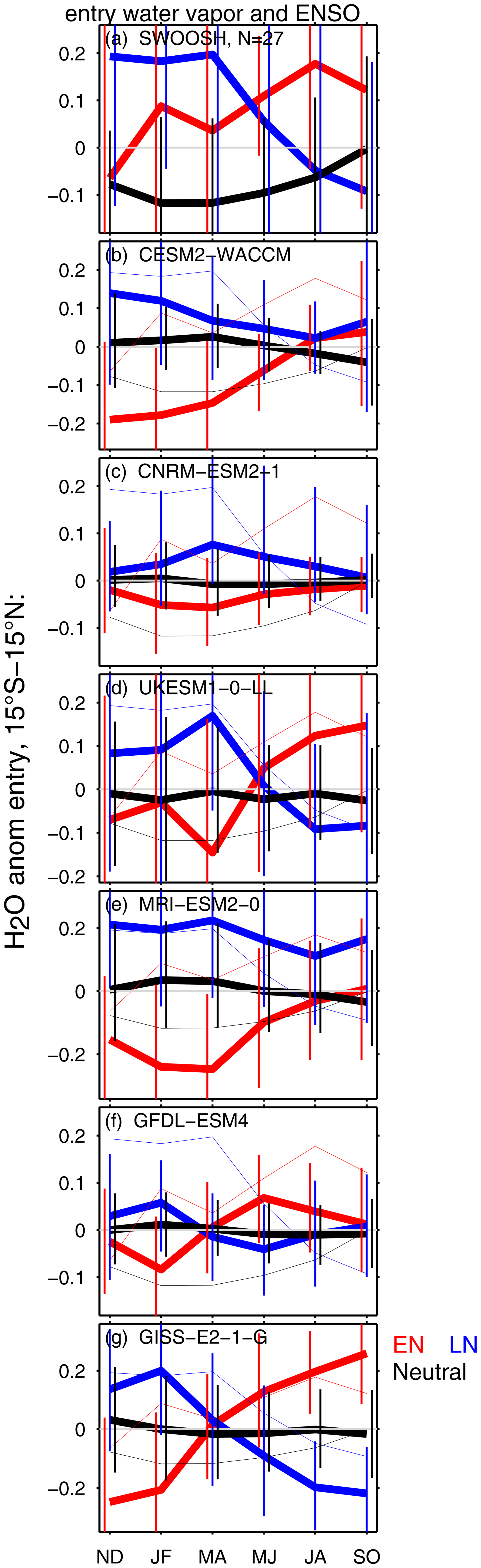
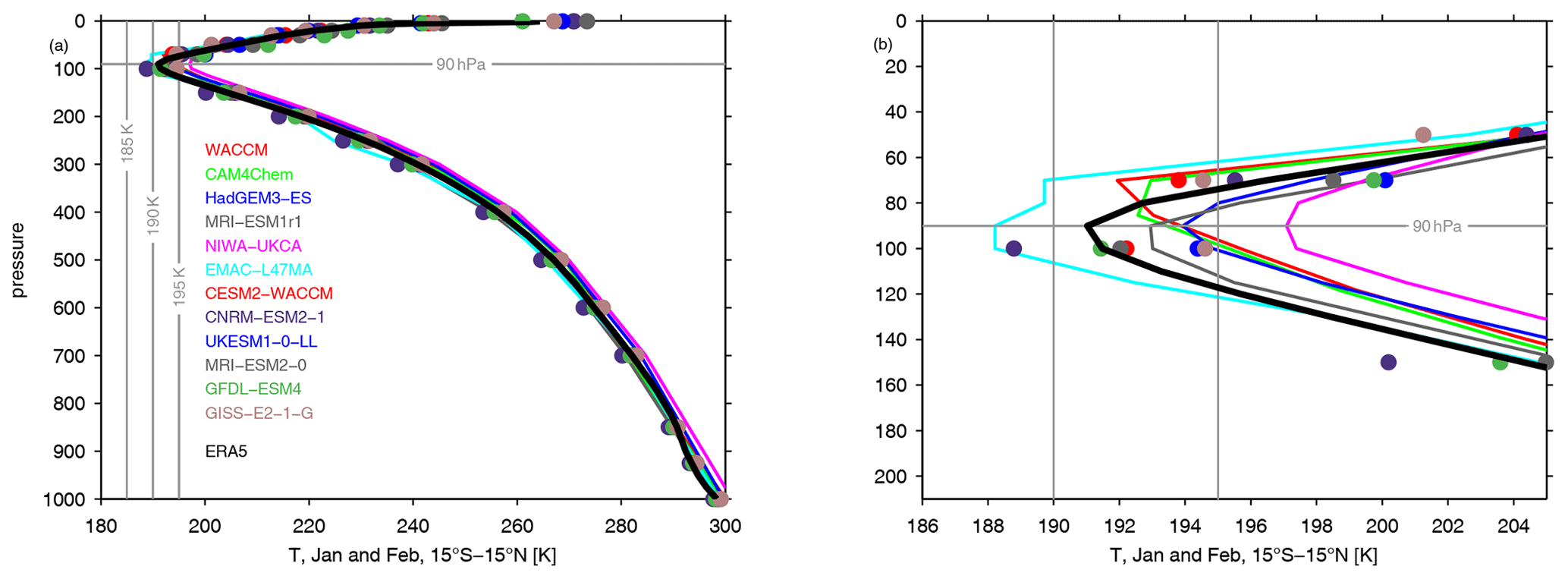
Figure 8Climatological mean temperature in January and February from 10∘ S to 10∘ N for each model and model level data from ERA5.1. Panel (b) enlarges the cold-point region from panel (a). For CMIP6 models, we only show the 100 and 70 hPa levels due to the limited resolution available in the CMIP data archive.
The standard deviation of 70 hPa tropical water vapor for each CMIP6 model is shown in Fig. 6b. While nearly all CCMI models struggled to capture realistic variability, half of the CMIP6 models simulate a realistic amount of variability. Specifically, the CCMI models HadGEM3-ES and MRI-ESM1r1 failed to simulate realistic variability in spring, but the corresponding CMIP6 models UKESM1-0-LL and MRI-ESM2-0 are realistic. GISS-E2-1-G also simulates a realistic amount of variability. However, the other three CMIP6 models simulate too little variability, although the bias in WACCM is smaller in the CMIP6 CESM2-WACCM than in the CCMI version of WACCM in winter.
Biases in the standard deviation of entry water have been shown to be associated with biases in cold-point temperature (Hardiman et al., 2015; Brinkop et al., 2016), and such an explanation can account for the biased variability in some of the models. Figure 8 shows the climatological zonal mean temperature from 10∘ S to 10∘ N in each model in January and February compared with ERA5.1. The NIWA model suffers from an overly warm cold point and, consistent with this, overly strong variability in entry water. EMAC-L47MA and CNRM-ESM2-1 suffer from the opposite problem: an overly cold cold point and too little variability in entry water. The Met Office model used in CMIP5 is known to have a warm cold-point bias (Hardiman et al., 2015), and this bias is somewhat reduced in CMIP6 (see blue line and circle in Fig. 8); this reduced bias is consistent with the improved variability in entry water. WACCM had a similar bias to the Met Office model in CCMI but was substantially improved for CMIP6 (see red circle and circle in Fig. 8), and water vapor variability is improved at least in midwinter. Not all models show a clear correspondence between cold-point and water vapor biases; however, the cold-point warm bias in the MRI model evident in CCMI was reduced in CMIP6, although water vapor variability increased, indicating that other confounding causes may be present.
More generally, there is still an overall tendency for models to have an overly warm cold point, similar to the bias in CMIP5 models (Hardiman et al., 2015), even as entry water vapor variability is generally too weak. These models may not yet adequately simulate all of the processes leading to observed variability in water vapor (e.g., ice lofting), or the models may not include all of the relevant forcing processes (e.g., aerosols in the Asian monsoon) that contribute to observed variability. Future work to improve models in this region of crucial importance for climate is clearly needed.
The amount of water vapor entering the stratosphere helps to determine the overall greenhouse effect and also regulates the severity of ozone depletion. The goal of this study is to understand how the comprehensive models that are used for the projection of future ozone and climate capture the connection between the dominant mode of interannual variability in the tropical troposphere, the El Niño–Southern Oscillation (ENSO), and entry stratospheric water vapor. That is, we follow the recommendation of Gettelman et al. (2001) and use ENSO as a natural experiment to study the fidelity of model-simulated variability in this region.
All models simulate a warmer tropical troposphere and cooler tropical lower stratosphere for El Niño (EN), the ENSO phase with anomalously warm sea surface temperatures in the tropical East Pacific (consistent with previous modeling and observational studies; Free and Seidel, 2009; Calvo et al., 2010; Simpson et al., 2011). Furthermore, EN leads to a zonal dipole in temperature anomalies near the tropopause in these models, with anomalously warm temperatures over the Indo-Pacific warm pool and anomalously cold temperatures over the Central Pacific (again consistent with the observed effect and previous modeling studies; Yulaeva and Wallace, 1994; Randel et al., 2000; Zhou et al., 2001; Scherllin-Pirscher et al., 2012; Domeisen et al., 2019). This is the first multi-model study to explore the subsequent effects on water vapor. While nearly all models (and observations) simulate a moistening for LN in winter and early spring compared with neutral ENSO, we find complex changes that differ in sign among the models for other seasons and for EN. Some models simulate enhanced water vapor for EN in both the winter of the event and the following spring, some models find an opposite response, and some show a nonlinear response, with both EN and LN leading to enhanced water vapor in spring. A moistening in the spring as the EN event decays, perhaps the strongest signal in observations, is simulated by only half of the models. A similarly wide diversity of responses is evident if we focus on Central Pacific ENSO vs. East Pacific ENSO or on temperatures in the mid-troposphere compared with temperatures near the surface. Despite this diversity in response, the temperature response near the cold point can explain the response of water vapor when each model is considered separately, with the response of temperatures in the coldest 20 % of the tropics to ENSO able to explain the simulated response to water vapor.
The observational record is too short to confidently classify models as “good” or “bad”, although most models simulate a response inconsistent with that observed even if we subsample their output to mimic the length of the observational record(Figs. 5 and 7). Furthermore, nearly all CCMI models and half of the CMIP6 models suffer from biases in the amount of interannual variability in entry water vapor, with most models simulating too little variability (Fig. 6). This bias in some models is due to biases in cold-point temperature, although it should be noted that, overall, the cold point is too warm in most models (Fig. 8 in this paper and Hardiman et al., 2015, for CMIP5). More generally, the overly weak variability could be due to biases in how the models simulate key processes regulating water vapor or due to missing forcings that lead to water vapor variability. Either way, the close correspondence between temperatures in the coldest 20 % of the tropics and the simulated water vapor response to ENSO (Table 2) suggests that the models resolve the most important factor governing entry water vapor variability (Mote et al., 1996; Hatsushika and Yamazaki, 2003; Fueglistaler et al., 2004; Fueglistaler and Haynes, 2005a; Oman et al., 2008; Randel and Park, 2019). The good news is that all three modeling groups that contributed to both CCMI and CMIP6 show an improvement in this bias. Future work is needed to fully consider what led to this improvement as well as to consider the impacts of these changes in the lowermost stratosphere on water vapor higher up.
The CCMI model output was retrieved from the Centre for Environmental Data Analysis (CEDA), the Natural Environment Research Council's Data Repository for Atmospheric Science and Earth Observation (https://data.ceda.ac.uk/badc/wcrp-ccmi/data/CCMI-1/output, Hegglin and Lamarque, 2015) and NCAR's Climate Data Gateway (https://www.earthsystemgrid.org/project/CCMI1.html, National Centre for Atmospheric Research, 2021).
The supplement related to this article is available online at: https://doi.org/10.5194/acp-21-3725-2021-supplement.
CIG designed the study, performed the analysis of the CMIP6 data, completed the analysis of the CCMI data, and wrote the paper. OH performed the initial analysis of the CCMI data. SZZ helped with the design of the methodology to isolate the ENSO signal and provided model level data for ERA5. JR assisted with the CMIP6 data. OH, OM, GZ, ST, DK, FMO, NB, MD, PJ, AP, and SD contributed CCMI data to the BADC archive or SWOOSH data.
The authors declare that they have no conflict of interest.
This article is part of the special issue “Chemistry–Climate Modelling Initiative (CCMI) (ACP/AMT/ESSD/GMD inter-journal SI)”. It is not associated with a conference.
We thank the international modeling groups for making their simulations available for this analysis, the joint WCRP SPARC/IGAC CCMI for organizing and coordinating the model data analysis activity, and the British Atmospheric Data Centre (BADC) for collecting and archiving the CCMI model output. Olaf Morgenstern and Guang Zeng acknowledge the UK Met Office for use of the Unified Model, the New Zealand Government’s Strategic Science Investment Fund (SSIF), and the contribution of NeSI high-performance computing facilities to the results of this research. DKRZ and its scientific steering committee are gratefully acknowledged for providing the high-performance computing and data-archiving resources for the ESCiMo (“Earth System Chemistry integrated Modelling”) consortial project. Computing and data storage resources, including the Cheyenne supercomputer, were provided by the Computational and Information Systems Laboratory (CISL) at NCAR. Correspondence should be addressed to Chaim I. Garfinkel (email: chaim.garfinkel@mail.huji.ac.il).
Chaim I. Garfinkel was supported by a European Research Council starting grant under the European Union's Horizon 2020 Research and Innovation program (grant no. 677756). Fiona M. O'Connor and the development of HadGEM3-ES was supported by the joint DECC/Defra Met Office Hadley Centre Climate Programme (grant no. GA01101) and by the European Commission's 7th Framework Programme (grant no. 603557; StratoClim project).
The EMAC simulations were performed at the German Climate Computing Center (DKRZ) and were financially supported by the Bundesministerium für Bildung und Forschung (BMBF).
The CESM project is primarily supported by the National Science Foundation (NSF). This material is based upon work supported by the National Center for Atmospheric Research, which is a major facility sponsored by the NSF under cooperative agreement no. 1852977.
Olaf Morgenstern received funding from the New Zealand Royal Society Marsden Fund (grant no. 12-NIW-006), and Makoto Deushi received funding from the Japan Society for the Promotion of Science (grant no. JP20K04070).
This paper was edited by Peter Hess and reviewed by Qinghua Ding and one anonymous referee.
Avery, M. A., Davis, S. M., Rosenlof, K. H., Ye, H., and Dessler, A.: Large anomalies in lower stratospheric water vapor and ice during the 2015–2016 El Nino, Nat. Geosci., 10, 405–409, https://doi.org/10.1038/ngeo2961, 2017. a
Banerjee, A., Chiodo, G., Previdi, M., Ponater, M., Conley, A. J., and Polvani, L. M.: Stratospheric water vapor: an important climate feedback, Clim. Dynam., 53, 1697–1710, 2019. a
Bonazzola, M. and Haynes, P.: A trajectory-based study of the tropical tropopause region, J. Geophys. Res.-Atmos., 109, D20112, https://doi.org/10.1029/2003JD004356, 2004. a
Brinkop, S., Dameris, M., Jöckel, P., Garny, H., Lossow, S., and Stiller, G.: The millennium water vapour drop in chemistry–climate model simulations, Atmos. Chem. Phys., 16, 8125–8140, https://doi.org/10.5194/acp-16-8125-2016, 2016. a, b, c
Calvo, N., Garcia, R., Randel, W., and Marsh, D.: Dynamical mechanism for the increase in tropical upwelling in the lowermost tropical stratosphere during warm ENSO events, J. Atmos. Sci., 67, 2331–2340, 2010. a, b, c
Chatterjee, S. and Hadi, A. S.: Regression analysis by example, John Wiley & Sons, New York, 2012. a
Davis, S. M., Rosenlof, K. H., Hassler, B., Hurst, D. F., Read, W. G., Vömel, H., Selkirk, H., Fujiwara, M., and Damadeo, R.: The Stratospheric Water and Ozone Satellite Homogenized (SWOOSH) database: a long-term database for climate studies, Earth Syst. Sci. Data, 8, 461–490, https://doi.org/10.5194/essd-8-461-2016, 2016. a, b
Deser, C., Simpson, I. R., McKinnon, K. A., and Phillips, A. S.: The Northern Hemisphere extratropical atmospheric circulation response to ENSO: How well do we know it and how do we evaluate models accordingly?, J. Climate, 30, 5059–5082, 2017. a
Dessler, A., Schoeberl, M., Wang, T., Davis, S., and Rosenlof, K.: Stratospheric water vapor feedback, P. Natl. Acad. Sci. USA, 110, 18087–18091, 2013. a
Dessler, A., Schoeberl, M., Wang, T., Davis, S., Rosenlof, K., and Vernier, J.-P.: Variations of stratospheric water vapor over the past three decades, J. Geophys. Res.-Atmos., 119, 12588–12598, https://doi.org/10.1002/2014JD021712, 2014. a
Dessler, A. E., Schoeberl, M. R., Wang, T., Davis, S. M., and Rosenlof, K. H.: Stratospheric water vapor feedback, P. Natl. Acad. Sci., 110, 18087–18091, https://doi.org/10.1073/pnas.1310344110, 2013. a
Diallo, M., Riese, M., Birner, T., Konopka, P., Müller, R., Hegglin, M. I., Santee, M. L., Baldwin, M., Legras, B., and Ploeger, F.: Response of stratospheric water vapor and ozone to the unusual timing of El Niño and the QBO disruption in 2015–2016, Atmos. Chem. Phys., 18, 13055–13073, https://doi.org/10.5194/acp-18-13055-2018, 2018. a
Ding, Q. and Fu, Q.: A warming tropical central Pacific dries the lower stratosphere, Clim. Dynam., 50, 2813–2827, 2018. a, b
Domeisen, D. I., Garfinkel, C. I., and Butler, A. H.: The teleconnection of El Niño Southern Oscillation to the stratosphere, Rev. Geophys., 57, 5–47, 2019. a, b
Dunne, J. P., Horowitz, L. W., Adcroft, A. J., Ginoux, P., Held, I. M., John, J. G., Krasting, J. P., Malyshev, S., Naik, V., Paulot, F., Shevliakova, E., Stock, C. A., Zadeh, N., Balaji, V., Blanton, C., Dunne, K. A., Dupuis, C., Durachta, J., Dussin, R., Gauthier, P. P. G., Griffies, S. M., Guo, H., Hallberg, R. W., Harrison, M., He, J., Hurlin, W., McHugh, C., Menzel, R., Milly, P. C. D., Nikonov, S., Paynter, D. J., Ploshay, J., Radhakrishnan, A., Rand, K., Reichl, B. G., Robinson, T., Schwarzkopf, D. M., Sentman, L. T., Underwood, S., Vahlenkamp, H., Winton, M., Wittenberg, A. T., Wyman, B., Zeng, Y., and Zhao, M.: The GFDL Earth System Model version 4.1 (GFDL-ESM4. 1): Model description and simulation characteristics, J. Adv. Model. Earth Sy., 11, 3167–3211, 2019. a, b
Dvortsov, V. L. and Solomon, S.: Response of the stratospheric temperatures and ozone to past and future increases in stratospheric humidity, J. Geophy. Res.-Atmos., 106, 7505–7514, 2001. a
Eyring, V., Arblaster, J. M., Cionni, I., Sedláček, J., Perlwitz, J., Young, P. J., Bekki, S., Bergmann, D., Cameron‐Smith, P., Collins, W. J., Faluvegi, G., Gottschaldt, K.-D., Horowitz, L. W., Kinnison, D. E., Lamarque, J.-F., Marsh, D. R., Saint‐Martin, D., Shindell, D. T., Sudo, K., Szopa, S., and Watanabe, S.: Long-term ozone changes and associated climate impacts in CMIP5 simulations, J. Geophys. Res.-Atmos., 118, 5029–5060, https://doi.org/10.1002/jgrd.50316, 2013. a, b
Eyring, V., Bony, S., Meehl, G. A., Senior, C. A., Stevens, B., Stouffer, R. J., and Taylor, K. E.: Overview of the Coupled Model Intercomparison Project Phase 6 (CMIP6) experimental design and organization, Geosci. Model Dev., 9, 1937–1958, https://doi.org/10.5194/gmd-9-1937-2016, 2016. a
Forster, P. M. and Shine, K. P.: Stratospheric water vapor changes as a possible contributor to observed stratospheric cooling, Geophys. Res. Lett., 26, 3309–3312, https://doi.org/10.1029/1999GL010487, 1999. a
Free, M. and Seidel, D. J.: Observed El Niño-Southern Oscillation temperature signal in the stratosphere, J. Geophys. Res., 114, D23108, https://doi.org/10.1029/2009JD012420, 2009. a, b
Fueglistaler, S. and Haynes, P.: Control of interannual and longer-term variability of stratospheric water vapor, J. Geophys. Res., 110, D24108, https://doi.org/10.1029/2005JD006019, 2005a. a, b, c
Fueglistaler, S. and Haynes, P.: Control of interannual and longer-term variability of stratospheric water vapor, J. Geophys. Res.-Atmos., 110, D24108, https://doi.org/10.1029/2005JD006019, 2005b. a
Fueglistaler, S., Wernli, H., and Peter, T.: Tropical troposphere-to-stratosphere transport inferred from trajectory calculations, J. Geophys. Res.-Atmos., 109, D03108, https://doi.org/10.1029/2003JD004069, 2004. a, b, c
Fueglistaler, S., Dessler, A. E., Dunkerton, T. J., Folkins, I., Fu, Q., and Mote, P. W.: Tropical tropopause layer, Rev. Geophys., 47, RG1004, https://doi.org/10.1029/2008RG000267, 2009. a
Fujiwara, M., Vömel, H., Hasebe, F., Shiotani, M., Ogino, S.-Y., Iwasaki, S., Nishi, N., Shibata, T., Shimizu, K., Nishimoto, E., Valverde Canossa, J. M., Selkirk, H. B., and Oltmans, S. J.: Seasonal to decadal variations of water vapor in the tropical lower stratosphere observed with balloon-borne cryogenic frost point hygrometers, J. Geophys. Res.-Atmos., 115, D18304, https://doi.org/10.1029/2010JD014179, 2010. a
Garcia, R. R., Smith, A. K., Kinnison, D. E., Cámara, Á. d. l., and Murphy, D. J.: Modification of the Gravity Wave Parameterization in the Whole Atmosphere Community Climate Model: Motivation and Results, J. Atmos. Sci., 74, 275–291, 2017. a
Garfinkel, C. I., Hurwitz, M., Oman, L., and Waugh, D. W.: Contrasting Effects of Central Pacific and Eastern Pacific El Nino on Stratospheric Water Vapor, Geophys. Res. Lett., 40, 4115–4120, 2013. a, b, c
Garfinkel, C. I., Gordon, A., Oman, L. D., Li, F., Davis, S., and Pawson, S.: Nonlinear response of tropical lower-stratospheric temperature and water vapor to ENSO, Atmos. Chem. Phys., 18, 4597–4615, https://doi.org/10.5194/acp-18-4597-2018, 2018. a, b, c, d, e, f, g, h
Garfinkel, C. I., Weinberger, I., White, I. P., Oman, L. D., Aquila, V., and Lim, Y.-K.: The salience of nonlinearities in the boreal winter response to ENSO: North Pacific and North America, Clim. Dynam., 52, 4429–4446, 2019. a
Gettelman, A., Randel, W., Massie, S., Wu, F., Read, W., and Russell III, J.: El Nino as a natural experiment for studying the tropical tropopause region, J. Climate, 14, 3375–3392, 2001. a, b, c
Gettelman, A., Mills, M. J., Kinnison, D. E., Garcia, R. R., Smith, A. K., Marsh, D. R., Tilmes, S., Vitt, F., Bardeen, C. G., McInerny, J., Liu, H.-L., Solomon, S. C., Polvani, L. M., Emmons, L. K., Lamarque, J.-F., Richter, J. H., Glanville, A. S., Bacmeister, J. T., Phillips, A. S., Neale, R. B., Simpson, I. R., DuVivier, A. K., Hodzic, A., and Randel, W. J.: The Whole Atmosphere Community Climate Model Version 6 (WACCM6), J. Geophys. Res.-Atmos., 124, 12380–12403, https://doi.org/10.1029/2019JD030943, 2019. a, b
Harari, O., Garfinkel, C. I., Ziskin Ziv, S., Morgenstern, O., Zeng, G., Tilmes, S., Kinnison, D., Deushi, M., Jöckel, P., Pozzer, A., O'Connor, F. M., and Davis, S.: Influence of Arctic stratospheric ozone on surface climate in CCMI models, Atmos. Chem. Phys., 19, 9253–9268, https://doi.org/10.5194/acp-19-9253-2019, 2019. a
Hardiman, S. C., Butchart, N., Haynes, P. H., and Hare, S. H. E.: A note on forced versus internal variability of the stratosphere, Geophys. Res. Lett., 34, L12803, https://doi.org/10.1029/2007GL029726, 2007. a
Hardiman, S. C., Boutle, I. A., Bushell, A. C., Butchart, N., Cullen, M. J. P., Field, P. R., Furtado, K., Manners, J. C., Milton, S. F., Morcrette, C., O'Connor, F. M., Shipway, B. J., Smith, C., Walters, D. N., Willett, M. R., Williams, K. D., Wood, N., Abraham, N. L., Keeble, J., Maycock, A. C., Thuburn, J., and Woodhouse, M. T.: Processes controlling tropical tropopause temperature and stratospheric water vapor in climate models, J. Climate, 28, 6516–6535, 2015. a, b, c, d
Hardiman, S. C., Butchart, N., O'Connor, F. M., and Rumbold, S. T.: The Met Office HadGEM3-ES chemistry–climate model: evaluation of stratospheric dynamics and its impact on ozone, Geosci. Model Dev., 10, 1209–1232, https://doi.org/10.5194/gmd-10-1209-2017, 2017. a
Hatsushika, H. and Yamazaki, K.: Stratospheric drain over Indonesia and dehydration within the tropical tropopause layer diagnosed by air parcel trajectories, J. Geophys. Res.-Atmos., 108, 4610, https://doi.org/10.1029/2002JD002986, 2003. a, b, c
Hegglin, M. I. and Lamarque, J.-F.: The IGAC/SPARC Chemistry-Climate Model Initiative Phase-1 (CCMI-1) model data output, NCAS British Atmospheric Data Centre, available at: https://data.ceda.ac.uk/badc/wcrp-ccmi/data/CCMI-1/output (last access: 10 March 2021), 2015. a
Hersbach, H., Bell, B., Berrisford, P., Hirahara, S., Horányi, A., Muñoz-Sabater, J., Nicolas, J., Peubey, C., Radu, R., Schepers, D., Simmons, A., Soci, C., Abdalla, S., Abellan, X., Balsamo, G., Bechtold, P., Biavati, G., Bidlot, J., Bonavita, M., De Chiara, G., Dahlgren, P., Dee, D., Diamantakis, M., Dragani, R., Flemming, J., Forbes, R., Fuentes, M., Geer, A., Haimberger, L., Healy, S., Hogan, R. J., Hólm, E., Janisková, M., Keeley, S., Laloyaux, P., Lopez, P., Lupu, C., Radnoti, G., de Rosnay, P., Rozum, I., Vamborg, F., Villaume, S., and Thépaut, J.-N.: The ERA5 Global Reanalysis, Q. J. Roy. Meteor. Soc., 146, 1999–2049, https://doi.org/10.1002/qj.3803, 2020. a, b, c
Jöckel, P., Tost, H., Pozzer, A., Kunze, M., Kirner, O., Brenninkmeijer, C. A. M., Brinkop, S., Cai, D. S., Dyroff, C., Eckstein, J., Frank, F., Garny, H., Gottschaldt, K.-D., Graf, P., Grewe, V., Kerkweg, A., Kern, B., Matthes, S., Mertens, M., Meul, S., Neumaier, M., Nützel, M., Oberländer-Hayn, S., Ruhnke, R., Runde, T., Sander, R., Scharffe, D., and Zahn, A.: Earth System Chemistry integrated Modelling (ESCiMo) with the Modular Earth Submodel System (MESSy) version 2.51, Geosci. Model Dev., 9, 1153–1200, https://doi.org/10.5194/gmd-9-1153-2016, 2016. a
Kawatani, Y., Lee, J. N., and Hamilton, K.: Interannual Variations of Stratospheric Water Vapor in MLS Observations and Climate Model Simulations, J. Atmos. Sci., 71, 4072–4085, https://doi.org/10.1175/JAS-D-14-0164.1, 2014. a
Keeble, J., Hassler, B., Banerjee, A., Checa-Garcia, R., Chiodo, G., Davis, S., Eyring, V., Griffiths, P. T., Morgenstern, O., Nowack, P., Zeng, G., Zhang, J., Bodeker, G., Cugnet, D., Danabasoglu, G., Deushi, M., Horowitz, L. W., Li, L., Michou, M., Mills, M. J., Nabat, P., Park, S., and Wu, T.: Evaluating stratospheric ozone and water vapor changes in CMIP6 models from 1850–2100, Atmos. Chem. Phys. Discuss. [preprint], https://doi.org/10.5194/acp-2019-1202, in review, 2020. a
Kelley, M., Schmidt, G. A., Nazarenko, L. S., Bauer, S. E., Ruedy, R., Russell, G. L., Ackerman, A. S., Aleinov, I., Bauer, M., Bleck, R., Canuto, V., Cesana, G., Cheng, Y., Clune, T. L., Cook, B. I., Cruz, C. A., Del Genio, A. D., Elsaesser, G. S., Faluvegi, G., Kiang, N. Y., Kim, D., Lacis, A. A., Leboissetier, A., LeGrande, A. N., Lo, K. K., Marshall, J., Matthews, E. E., McDermid, S., Mezuman, K., Miller, R. L., Murray, L. T., Oinas, V., Orbe, C., García-Pando, C. P., Perlwitz, J. P., Puma, M. J., Rind, D., Romanou, A., Shindell, D. T., Sun, S., Tausnev, N., Tsigaridis, K., Tselioudis, G., Weng, E., Wu, J., adnd Yao, M. S.: GISS-E2. 1: Configurations and Climatology, J. Adv. Model. Earth Sy., e2019MS002025, https://doi.org/10.1029/2019MS002025, 2019. a, b
Konopka, P., Ploeger, F., Tao, M., and Riese, M.: Zonally resolved impact of ENSO on the stratospheric circulation and water vapor entry values, J. Geophys. Res.-Atmos., 121, 11486–11501, https://doi.org/10.1002/2015JD024698, 2016. a, b
Levine, J. G., Braesicke, P., Harris, N. R. P., Savage, N. H., and Pyle, J. A.: Pathways and timescales for troposphere-to-stratosphere transport via the tropical tropopause layer and their relevance for very short lived substances, J. Geophys. Res.-Atmos., 112, D04308 https://doi.org/10.1029/2005JD006940, 2007. a
Li, F. and Newman, P.: Stratospheric water vapor feedback and its climate impacts in the coupled atmosphere–ocean Goddard Earth Observing System Chemistry-Climate Model, Clim. Dynam., 55, 1585–1595, https://doi.org/10.1007/s00382-020-05348-6, 2020. a
Liang, C., Eldering, A., Gettelman, A., Tian, B., Wong, S., Fetzer, E., and Liou, K.: Record of tropical interannual variability of temperature and water vapor from a combined AIRS-MLS data set, J. Geophys. Res., 116, D06103, https://doi.org/10.1029/2010JD014841, 2011. a
Meinshausen, M., Smith, S. J., Calvin, K., Daniel, J. S., Kainuma, M. L. T., Lamarque, J.-F., Matsumoto, K., Montzka, S. A., Raper, S. C. B., Riahi, K., Thomson, A., Velders, G. J. M., and van Vuuren, D. P. P.: The RCP greenhouse gas concentrations and their extensions from 1765 to 2300, Clim. Change, 109, 213–241, 2011. a, b
Morgenstern, O., Braesicke, P., O'Connor, F. M., Bushell, A. C., Johnson, C. E., Osprey, S. M., and Pyle, J. A.: Evaluation of the new UKCA climate-composition model – Part 1: The stratosphere, Geosci. Model Dev., 2, 43–57, https://doi.org/10.5194/gmd-2-43-2009, 2009. a
Morgenstern, O., Hegglin, M. I., Rozanov, E., O'Connor, F. M., Abraham, N. L., Akiyoshi, H., Archibald, A. T., Bekki, S., Butchart, N., Chipperfield, M. P., Deushi, M., Dhomse, S. S., Garcia, R. R., Hardiman, S. C., Horowitz, L. W., Jöckel, P., Josse, B., Kinnison, D., Lin, M., Mancini, E., Manyin, M. E., Marchand, M., Marécal, V., Michou, M., Oman, L. D., Pitari, G., Plummer, D. A., Revell, L. E., Saint-Martin, D., Schofield, R., Stenke, A., Stone, K., Sudo, K., Tanaka, T. Y., Tilmes, S., Yamashita, Y., Yoshida, K., and Zeng, G.: Review of the global models used within phase 1 of the Chemistry–Climate Model Initiative (CCMI), Geosci. Model Dev., 10, 639–671, https://doi.org/10.5194/gmd-10-639-2017, 2017. a, b
Mote, P. W., Rosenlof, K. H., McIntyre, M. E., Carr, E. S., Gille, J. C., Holton, J. R., Kinnersley, J. S., Pumphrey, H. C., Russell III, J. M., and Waters, J. W.: An atmospheric tape recorder: The imprint of tropical tropopause temperatures on stratospheric water vapor, J. Geophys. Res.-Atmos., 101, 3989–4006, 1996. a, b, c, d
National Centre for Atmospheric Research: CCMI Phase 1, available at: https://www.earthsystemgrid.org/project/CCMI1.html, last access: 10 March 2021. a
Oman, L., Waugh, D. W., Pawson, S., Stolarski, R. S., and Nielsen, J. E.: Understanding the Changes of Stratospheric Water Vapor in Coupled Chemistry-Climate Model Simulations, J. Atmos. Sci., 65, 3278, https://doi.org/10.1175/2008JAS2696.1, 2008. a, b
Randel, W. and Park, M.: Diagnosing observed stratospheric water vapor relationships to the cold point tropical tropopause, J. Geophys. Res.-Atmos., 124, 7018–7033, 2019. a, b, c
Randel, W. J., Wu, F., and Gaffen, D. J.: Interannual variability of the tropical tropopause derived from radiosonde data and NCEP reanalyses, J. Geophys. Res., 105, 15509–15523, 2000. a, b
Rao, J., Garfinkel, C. I., and White, I. P.: Impact of the Quasi-Biennial Oscillation on the Northern Winter Stratospheric Polar Vortex in CMIP5/6 Models, J. Climate, 33, 4787–4813, https://doi.org/10.1175/JCLI-D-19-0663.1, 2020a. a
Rao, J., Garfinkel, C. I., and White, I. P.: How does the Quasi-Biennial Oscillation affect the boreal winter tropospheric circulation in CMIP5/6 models?, J. Climate, 33, 8975–8996, 2020b. a
Reid, G. C. and Gage, K. S.: Interannual variations in the height of the tropical tropopause, J. Geophys. Res.-Atmos., 90, 5629–5635, 1985. a
Richter, J. H., Anstey, J. A., Butchart, N., Kawatani, Y., Meehl, G. A., Osprey, S., and Simpson, I. R.: Progress in Simulating the Quasi-Biennial Oscillation in CMIP Models, J. Geophys. Res.-Atmos., 125, e2019JD032362, https://doi.org/10.1029/2019JD032362, 2020. a
Scaife, A. A., Butchart, N., Jackson, D. R., and Swinbank, R.: Can changes in ENSO activity help to explain increasing stratospheric water vapor?, Geophys. Res. Lett., 30, 1880, https://doi.org/10.1029/2003GL017591, 2003. a
Scherllin-Pirscher, B., Deser, C., Ho, S.-P., Chou, C., Randel, W., and Kuo, Y.-H.: The vertical and spatial structure of ENSO in the upper troposphere and lower stratosphere from GPS radio occultation measurements, Geophys. Res. Lett., 39, L20801, https://doi.org/10.1029/2012GL053071, 2012. a, b
Séférian, R., Nabat, P., Michou, M., Saint‐Martin, D., Voldoire, A., Colin, J., Decharme, B., Delire, C., Berthet, S., Chevallier, M., and Sénési, S.: Evaluation of CNRM Earth System Model, CNRM-ESM2-1: Role of Earth System Processes in Present-Day and Future Climate, J. Adv. Model. Earth Sy., 11, 4182–4227, 2019. a, b
Sellar, A. A., Jones, C. G., Mulcahy, J. P., Tang, Y., Yool, A., Wiltshire, A., O'Connor, F. M., Stringer, M., Hill, R., Palmieri, J., Woodward, S., de Mora, L., Kuhlbrodt, T., Rumbold, S. T., Kelley, D. I., Ellis, R., Johnson, C. E., Walton, J., Abraham, N. L., Andrews, M. B., Andrews, T., Archibald, A. T., Berthou, S., Burke, E., Blockley, E., Carslaw, K., Dalvi, M., Edwards, J., Folberth, G. A., Gedney, N., Griffiths, P. T., Harper, A. B., Hendry, M. A., Hewitt, A. J., Johnson, B., Jones, A., Jones, C. D., Keeble, J., Liddicoat, S., Morgenstern, O., Parker, R. J., Predoi, V., Robertson, E., Siahaan, A., Smith, R. S., Swaminathan, R., Woodhouse, M. T., Zeng, G., and Zerroukat, M.: UKESM1: Description and Evaluation of the U.K. Earth System Model, J. Adv. Model. Earth Sy., 11, 4513–4558, https://doi.org/10.1029/2019MS001739, 2019. a, b
Simpson, I. R., Shepherd, T. G., and Sigmond, M.: Dynamics of the lower stratospheric circulation response to ENSO, J. Atmos. Sci., 68, 2537–2556, 2011. a, b
Solomon, S., Garcia, R. R., Rowland, F. S., and Wuebbles, D. J.: On the depletion of Antarctic ozone, Nature, 321, 755–758, https://doi.org/10.1038/321755a0, 1986. a
Solomon, S., Rosenlof, K. H., Portmann, R. W., Daniel, J. S., Davis, S. M., Sanford, T. J., and Plattner, G.-K.: Contributions of Stratospheric Water Vapor to Decadal Changes in the Rate of Global Warming, Science, 327, 1219–1223, https://doi.org/10.1126/science.1182488, 2010. a
SPARC-CCMVal: SPARC Report on the Evaluation of Chemistry-Climate Models, SPARC Report, 5, WCRP-132, WMO/TD-No. 1526, available at: https://www.sparc-climate.org/publications/sparc-reports/sparc-report-no-5/ (last access: 4 March 2021), 2010. a
Tao, M., Konopka, P., Ploeger, F., Yan, X., Wright, J. S., Diallo, M., Fueglistaler, S., and Riese, M.: Multitimescale variations in modeled stratospheric water vapor derived from three modern reanalysis products, Atmos. Chem. Phys., 19, 6509–6534, https://doi.org/10.5194/acp-19-6509-2019, 2019. a, b
Tilmes, S., Lamarque, J.-F., Emmons, L. K., Kinnison, D. E., Marsh, D., Garcia, R. R., Smith, A. K., Neely, R. R., Conley, A., Vitt, F., Val Martin, M., Tanimoto, H., Simpson, I., Blake, D. R., and Blake, N.: Representation of the Community Earth System Model (CESM1) CAM4-chem within the Chemistry-Climate Model Initiative (CCMI), Geosci. Model Dev., 9, 1853–1890, https://doi.org/10.5194/gmd-9-1853-2016, 2016. a
Wang, C. and Fiedler, P. C.: ENSO variability and the eastern tropical Pacific: A review, Prog. Oceanogr., 69, 239–266, 2006. a
Wang, T., Zhang, Q., Hannachi, A., Hirooka, T., and Hegglin, M. I.: Tropical water vapour in the lower stratosphere and its relationship to tropical/extratropical dynamical processes in ERA5, Q. J. Roy. Meteor. Soc., 146, 2432–2449, https://doi.org/10.1002/qj.3801, 2020. a
Weinberger, I., Garfinkel, C. I., White, I. P., and Oman, L. D.: The salience of nonlinearities in the boreal winter response to ENSO: Arctic stratosphere and Europe, Clim. Dynam., 53, 4591–4610, 2019. a
World Meteorological Organization: Scientific Assessment of Ozone Depletion: 2010, Global Ozone Research and Monitoring Project Rep. No. 52, WMO, 2011. a
Yook, S., Thompson, D. W. J., Solomon, S., and Kim, S.-Y.: The key role of coupled chemistry-climate interactions in tropical stratospheric temperature variability, J. Climate, 33, 7619–7629, https://doi.org/10.1175/JCLI-D-20-0071.1, 2020. a
Yuan, W., Geller, M. A., and Love, P. T.: ENSO influence on QBO modulations of the tropical tropopause, Q. J. Roy. Meteor. Soc., 140, 1670–1676, https://doi.org/10.1002/qj.2247, 2014. a
Yukimoto, S., Adachi, Y., Hosaka, M., Sakami, T., Yoshimura, H., Hirabara, M., Tanaka, T. Y., Shindo, E., Tsujino, H., Deushi, M., and Mizuta, R.: A new global climate model of the Meteorological Research Institute: MRI-CGCM3-model description and basic performance, J. Meteorol. Soc. Jpn. Ser. II, 90, 23–64, https://doi.org/10.2151/jmsj.2012-A02, 2012. a
Yukimoto, S., Kawai, H., Koshiro, T., Oshima, N., Yoshida, K., Urakawa, S., Tsujino, H., Deushi, M., Tanaka, T., Hosaka, M., and Yabu, S.: The Meteorological Research Institute Earth System Model version 2.0, MRI-ESM2. 0: Description and basic evaluation of the physical component, J. Meteorol. Soc. Jpn. Ser. II, 97, 931–965, https://doi.org/10.2151/jmsj.2019-051, 2019. a, b
Yulaeva, E. and Wallace, J. M.: The signature of ENSO in global temperature and precipitation fields derived from the microwave sounding unit, J. Climate, 7, 1719–1736, 1994. a, b
Zhou, X. L., Geller, M. A., and Zhang, M. H.: Tropical cold point tropopause characteristics derived from ECMWF reanalyses and soundings, J. Climate, 14, 1823–1838, 2001. a, b, c, d
Zhou, X. L., Geller, M. A., and Zhang, M.: Temperature fields in the tropical tropopause transition layer, J. Climate, 17, 2901–2908, 2004. a, b